transport modeling of hydrogen in metals for application ... · transport modeling of hydrogen in...
TRANSCRIPT

Final Technical Report
Transport Modeling of Hydrogen in Metals forApplication to Hydrogen Assisted Cracking of
Metalsby
Dr. James P. Thomas (PI) and Mr. Charles E. Chopin
for theOffice of Naval Research
Grant Number: N00014-93-1-0845
DTICC ELECTE
OCT 1 6 1995
F Department of Aerdj'i-ce
and Mechahicai Engineering
University of Notre DameON • S N A Notre Dame, Indiana 46556
19951012 037
I i TR: 001-4/95

Final Technical Report
Transport Modeling of Hydrogen in Metals forApplication to Hydrogen Assisted Cracking of
Metalsby
Dr. James P. Thomas (PI) and Mr. Charles E. Chopin
for theOffice of Naval Research
Grant Number: N00014-93-1-0845
0 (
"TR " 001-4195

Final Technical Report
Transport Modeling of Hydrogen in Metalsfor Application to Hydrogen Assisted Cracking of Metals
submitted by:
Dr. James P. Thomast and Mr. Charles E. ChopintUniversity of Notre Dame
Department of Aerospace and Mechanical EngineeringNotre Dame, Indiana 46556-5637
April 4, 1995
submitted to:
Dr. A. John Sedriks, Code 3312
Office of Naval ResearchBallston Tower One
800 North Quincy StreetArlington, Virginia 22217-5660
Grant Number: N00014-93-1-0845September 1, 1993 to December 31, 1994
Principal Investigator, Assistant Professor.t Graduate Research Assistant
TABLE OF CONTENTS
ONR Contract Inform ation ............................................................................................... iiiExecutive Sum m ary ............................................................................................................... ivFinal Report ............................................................................................................................ 1
Introduction ................................................................................................................ 1Theoretical M odeling ............................................................................................... 3
Balance Equations ........................................................................................ 3Trapping Analysis ........................................................................................ 4Constitutive Equations .................................................................................. 4Governing Equations .................................................................................... 6
Finite Elem ent M odeling ......................................................................................... 6Programm ing Sim plifications ...................................................................... 7Formulation of the Finite Element Matrix Equations ................................... 8Interpolation Functions for the Concentration and Displacement ................ 8Isoparam etric Interpolation Functions ........................................................ 10Gauss-Legendre Num erical Integration ...................................................... 11Finite Elem ent Equations ........................................................................... 12N on-Linear Solutions via Newton-Raphson ............................................... 13Re-Ordering the Degrees of Freedom ........................................................ 14AB AQUS User Elem ent Subroutines ........................................................ 15
M odeling Applications ........................................................................................... 16Results ....................................................................................................................... 17
Case 1 and 2 Problem s ............................................................................... 17Case 3 Problem s ......................................................................................... 21
D iscussion ................................................................................................................. 24Sum m ary and Future Research ........................................................................... 26
Acknowledgm ents ................................................................................................................. 27References ............................................................................................................................. 28
Appendix A : Analytical Solutions via M aple .................................................................. A-]Appendix B: User Elem ent Subroutine ........................................................................... B-1Appendix C: Sample Input D eck .................................................................................... C-1Appendix D : Sample Output ........................................................................................... D -1Appendix E: Conference Paper ....................................................................................... E-1Appendix F: Summary of Publications/Reports/Presentations During Grant Period .... F-1
ii
ONR CONTRACT INFORMATION
Contract Title: "Transport Modeling of Hydrogen in MetalsFor Application to Hydrogen Assisted Cracking"
Performing Organization: University of Notre Dame
Principal Investigator: Dr. James P. Thomas
Contract Number: NOO 14-93-1-0845
R & T Project Number: cor5247---01
ONR Scientific Officer: Dr. A. John Sedriks, Code 3312
iii

EXECUTIVE SUMMARY
The focus of this research was on the development of a finite element code for solutetransport and trapping in linear elastic mixtures for use in modeling the hydrogen transportprocess in metals undergoing hydrogen assisted cracking. Specific objectives included:
1.) Completion of the development of a solute transport and trapping model withcoupling between the concentration, deformation, and thermal field variables andtrapping at reversible and irreversible trap sites.
2.) Implementation of the above theory in a finite element code.3.) Calculation of the crack tip deformations and chemical state variables for some high
strength steels under a variety of loading, environment, and material conditions.A solute transport model has been developed for linear elastic mixtures with coupling
between the deformation, concentration, and thermal variables and trapping at reversible andirreversible trap sites. A journal publication describing this model is in preparation 1.
Work on a 2-D finite element implementation and its application to the modeling ofhydrogen transport in a cracking metal is ongoing. A 1-D code has been developed and testedon a variety of problems with known analytical solutions. The "code" consists of a Fortran"user element" subroutine for use with the ABAQUS 2 finite element program.Documentation of the 1-D user element subroutine is contained within this report.
Work on objective 3.) could not be started without a 2-D version of the finite elementcode. The 1-D code was used to model a variety of hydrogen transport problems with theobjective of learning more about the fully coupled transport theory. We were able to "invent"a problem with a square-root singular stress (a, - 1/ Vx). This problem was used to gainpreliminary insight into the hydrogen distribution problem in planar crack geometries. Theproblem consisted of subjecting a 4340 steel rod (10 cm x 1 cm 2) to a singular body force (-1/x 3/2 ) resulting in the square root singular stress. The steady-state hydrogen concentrationsand deformations were determined using the fully coupled theory, developed in this work,and classical stress assisted diffusion (SAD) theory.
The fully coupled predictions showed slightly higher hydrogen concentrations, a moresevere singularity in the concentration, larger axial and dilatational strains, and larger axialdisplacements, all of which depended on the extent of hydrogen trapping. The mathematicalsolution for the concentration became multi-valued as the singularity was approached. It wasshown that this "non-physical" result would be eliminated if the product of the density, themolar volume of hydrogen in the mixture, and the bulk modulus decrease linearly or betterwith increasing hydrogen concentration. These findings are documented in the report and in aconference paper included as Appendix E.
Development of a 2-D user element subroutine is ongoing. The 2-D code will initiallybe limited to simple linear elastic mixture behavior and equilibrium trapping. Extensions ofthe model to include non-equilibrium trapping effects and plastic crack tip deformations areplanned. An effort is also being made to interface the ABAQUS code with our user elementroutines to the Patran 3 Solid Geometry Modeling program for more convenient meshing ofcomplex 2-D geometries and for displaying the finite element results.
I J. P. Thomas and P. Matic, "Solute Transport Modeling in Elastic Solids", Int. J. Engnr. Sci., in preparation.2 ABAQUS is a finite element code supported by HKS, Inc., Pawtucket, RI.3 Patran is a solid geometry modeling program supported by PDA Engineering, Costa Mesa, CA.
iv
TRANSPORT MODELING OF HYDROGEN IN METALSFOR APPLICATION TO HYDROGEN ASSISTED CRACKING
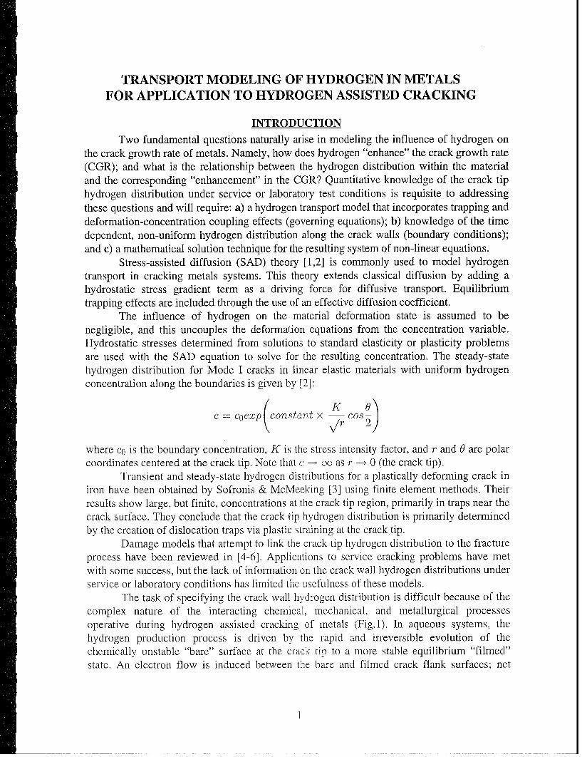
INTRODUCTIONTwo fundamental questions naturally arise in modeling the influence of hydrogen on
the crack growth rate of metals. Namely, how does hydrogen "enhance" the crack growth rate(CGR); and what is the relationship between the hydrogen distribution within the materialand the corresponding "enhancement" in the CGR? Quantitative knowledge of the crack tiphydrogen distribution under service or laboratory test conditions is requisite to addressingthese questions and will require: a) a hydrogen transport model that incorporates trapping anddeformation-concentration coupling effects (governing equations); b) knowledge of the timedependent, non-uniform hydrogen distribution along the crack walls (boundary conditions);and c) a mathematical solution technique for the resulting system of non-linear equations.
Stress-assisted diffusion (SAD) theory [1,2] is commonly used to model hydrogentransport in cracking metals systems. This theory extends classical diffusion by adding ahydrostatic stress gradient term as a driving force for diffusive transport. Equilibriumtrapping effects are included through the use of an effective diffusion coefficient.
The influence of hydrogen on the material deformation state is assumed to benegligible, and this uncouples the deformation equations from the concentration variable.Hydrostatic stresses determined from solutions to standard elasticity or plasticity problemsare used with the SAD equation to solve for the resulting concentration. The steady-statehydrogen distribution for Mode I cracks in linear elastic materials with uniform hydrogenconcentration along the boundaries is given by [2]:(K
c coCXp (consta•t x K/r cos0
where co is the boundary concentration, K is the stress intensity factor, and r and 0 are polarcoordinates centered at the crack tip. Note that c --* oc as r -* 0 (the crack tip).
Transient and steady-state hydrogen distributions for a plastically deforming crack iniron have been obtained by Sofronis & McMeeking [3] using finite element methods. Theirresults show large, but finite, concentrations at the crack tip region, primarily in traps near thecrack surface. They conclude that the crack tip hydrogen distribution is primarily determinedby the creation of dislocation traps via plastic straining at the crack tip.
Damage models that attempt to link the crack tip hydrogen distribution to the fractureprocess have been reviewed in [4-6]. Applications to service cracking problems have metwith some success, but the lack of information on the crack wall hydrogen distributions underservice or laboratory conditions has limited the usefulness of these models.
The task of specifying the crack wall hydrogen distribution is difficult because of thecomplex nature of the interacting chemical, mechanical, and metallurgical processesoperative during hydrogen assisted cracking of metals (Fig. 1). In aqueous systems, thehydrogen production process is driven by the rapid and irreversible evolution of thechemically unstable "bare" surface at the crack tip to a more stable equilibrium "filmed"state. An electron flow is induced between the bare and filmed crack flank surfaces; net

anodic (dissolution/filming) reactions take place on the bare surface and net cathodic(hydrogen reduction) reactions take place on the filmed surfaces.
Adsorbed hydrogen, Hads, can be produced on both the bare and filmed cracksurfaces by: (1) the reduction of hydrogen ions in acidic environments; or (2) by thereduction of water in alkaline environments. The MHod, species are then free to be absorbedby the transition reaction (a); or combine to form H 2 gas via: recombination (bl); orelectrochemical desorption (b2). Reactions (a), (bl), and (b2) occur in parallel, but one ofthe two (bl) or (b2) reactions is usually dominant (Fig.2).
Crack Tip RegionBare C-local
Steady State Film Coverage Film Growth Surface
Me
1. Electrochemical Mass Transport '71ocal2. Anodic and Cathodic Surface Reactions3. Hydrogen Absorption Reactions4. Hydrogen Transport and Trapping5. Hydrogen Damage
Figure 1: Schematic of the processes responsible for hydrogen assisted crack growth.
(1) Acidic: M + H+ + C- # MHads(2) Alkaline: M + H 20 + e- < MH~d + OH
(a) Adsorption-Absorption: MHads • MHaibs
(bl) Recombination: MH~d, + MHad• : H2 + 2M
(b2) EC Desorption: MHd + H+ + e6 4= H 2 + M
Figure 2: Summary of the hydrogen producing reactions.
The distribution of MHabs along the crack surface is governed by the surfacecoverage of MHad, and the kinetics of reaction (a) acting in parallel with reaction (bl) or(b2). These factors are influenced, in turn, by: the electrochemical environment at the cracktip region (e.g., the potential, pH, species concentrations, dissolved 02, etc.); the kinetics ofthe bare and filmed surface reactions; and the rate of transport of H~b, from the crack surfaceinto the material.
2

Iyer and Pickering [7] have reviewed and modeled the kinetics of hydrogen evolutionand entry in stress free metallic systems with homogeneous electrochemical conditions at themetal surface. Their model is used to quantify the rate constants associated with reactions (1)or (2) and (a) and (bl) or (b2) via analysis of experimental permeation data. Turnbull [8] hasreviewed electrochemical conditions in cracks with particular emphasis on corrosion fatiguecracks of structural steels in sea water. Similarly, Beck [9] and Newman [10] have examinedexperimental techniques for characterizing bare (and filmed) surface reaction kinetics. Theabove models, data, and techniques, plus information concerning the rate controlling processduring crack growth, will have to be used in an analysis of the mass transport process withinthe crack to develop realistic predictions of the MHabs distribution.
We begin with a description of fully coupled transport and trapping theory. The use ofthe ABAQUS finite element "User Element" subroutines for solving 1-D problems is thenoutlined in full detail. This is followed by a description of three 1-D rod problems that havebeen studied. The results of these studies are reported next, followed by a discussion. Andfinally, some conclusions are drawn, and suggestions are made for further research.
THEORETICAL MODELING
This section begins with a brief description of the theory adopted for modelingcoupled diffusion/trapping processes. Derivation of the finite element equations using themethod of weighted residuals is described, followed by a description of analytical and finiteelement solutions to three simple steady-state hydrogen transport problems. While themotivation for this work is the modeling of hydrogen transport in cracking metal systems, theformulation presented here is generalized to generic solute-solid mixtures.
Three solute species are modeled in the analysis:SL - interstitial or lattice species
SR = weak or moderately (reversibly) trapped speciesSr -_ strongly (irreversibly) trapped species
Balance EquationsBalance equations for the mixture mass, the three solute species masses, mixture
linear momentum and moment of momentum, mixture energy, and mixture entropy can bewritten. In this report, our modeling considerations will be restricted to isothermal linearelastic mixtures so that only the balance equations for the solute species mass and mixturelinear momentum need be explicitly considered. Assuming negligible inertial effects, they aregiven by:
Mass: u+ V a ( = L, R, or0 ) (1)
Linear Momentum: o7ijj + F, = 0 ( .j = y, , or z) (2)
where: ck -_ mass fraction concentrations for Sk [kg/kg].
Jk concentration flux vectors for Sk [kg/kg. rm/s].Sak •mass supply rates for Sk [kg/lkgs].aij - stress tensor [N/rn2 ].
Fj =- the it component of body force vector [N/M 3 ].
3

Trapping AnalysisExpressions for the mass supply rates ak in Eq. (1) are written in accordance with the
trapping model of McNabb & Foster [11]:
Stoichiometry: SL 4* SR and SL = Si (3)
The stoichiometric relations require the supply terms sum to zero (i.e., aR + ai - aL).
Kinetics of Trapping: aR =k k(1 - OR)CL - k'40R (4)
ai = k!f(1 - O0)CL - k'O, ,.z kf (1 -- OI)CLwhere: i4 ,kf, kb , kb4 = forward and backward trap rate constants for SR and S" [1/s].
0 R and 0- cR/CR and cI/ci, respectively, are the fraction of filled trap sites [1].cR and ces saturation mass fraction concentration of SR and S. [kg/kg].
The quantities kf, kf, k , k , c' and cs are related to trap site densities, probability ofcapture, etc. and can be quantified via experimental measurement (see, for example, [12-14]).
Significant simplifications are effected when the rate constants for trapping are muchgreater than those for diffusive transport. Trapping can then be modeled as a steady-stateprocess (i.e., a = aR =- ar = 0). This case is considered below.SS Trapping: CR =cR± KRf CL- R _T = C'(5)
1 + KR C,(k f AEbN
KR j eb-:xp~ /1kR
The total internal solute concentration is simply a linear function of CL (Xi, t):
CTOTAL (Xi, t) =CL (Xi, t) + CR (Xi, t) +±C c(Xi, t) =(1 + c' KR) CL (Xi, t) + C' (6)
The three versions of Eq. (1) (one for each species) can be summed to give a singleequation by the following considerations. First, JR = J, = 0 because of the linear elasticmaterial assumption which precludes trap site motion (e.g., dislocation motion during plasticdeformation). Second, from Eq. (5a):
OCft &CL acic0 CR S I-- and -- 0 (7)
at at at
Summation of the three balances results in the following single mass balance equation:
S+ OCL ' (8)at
Constitutive Equations
Mass Flux: JcL CL V/LIL Linear Onsager Relation (9)R'L T
where [IL is a mass based chemical potential [15] defined by:
4

1L = 1, (°L(T) + RTln(cL) - Vske) (10)ML L L kg (10)19L ML
and: DL diffusion coefficient for SL [mr2/s].
RL gas constant for SL = R/ML [J/kg 'K].
ML = molecular mass of SL [kg/mol].T temperature [0K].
S=---(CL, CR, c-; cjj; T) free energy per unit mixture mass [J/kg].It'(T) = reference potential for SL at temperature T [J/rnol].
V, - partial molar volume of solute in the metal [m 3/mol S].
k bulk modulus of elasticity [N/mr2].
e trace of the strain tensor (i.e., e = Eii = ±ll + E22 + E33) [m/m].
The use of a mass based chemical potential simplifies the analysis of fully coupleddeformation-diffusion processes because of the primary role played by mass in thedeformation equations.
The resulting expression for concentration flux is given by:
JL DL Vs D+_L_ kcLVe (11)-DLVCL±IRT
The constitutive equation for the stress consists of Hooke's law combined with adilatational stress contribution due to changes in the total solute concentration:
Stress: ij = P a A e 6ij + 2G6ij - 3k a, (1 + c' KR) ACL 6ij (12)
where: p mass density of the solid [kg/m 3 ].
A Lame' constant [N/mr2].ij- Kronecker delta (6ij = 1 for i j and 0 otherwise).
G shear modulus [N/mr2].
- (ui,j + uj,j) infinitesimal strain tensor [m/m].
ui the ith component of the displacement vector Irn].a, - linear expansion coefficient for internal solute = 1 k4A
3 ML r/nA]ACL - CL - cO = change in cLfrom the reference level, co.
(1 + c' KR)ACL -- change in Ctotal from the reference level.
The influence of the irreversibly trapped solute on the deformation of the solid hasbeen ignored in Eq. (12). The assumption of equilibrium trapping implies that ci-- -*c
immediately upon introducing solute into the solid. We have assumed, therefore, thatc, = c', and that all deformations are measured with respect to an initial uniformdeformation arising from the presence of the irreversibly trapped solute species at itssaturation concentration level.
5

The relationship between the chemical potential and stress (Eqs. (10) and (12)) is
dictated by the thermodynamic reciprocity relationship:
a/IL _ o(ij/P) (13)
Dcij DCL
The equations of classical stress assisted diffusion violate this requirement by ignoring theconcentration induced dilatational stresses.
Governing EquationsCombining the mass and momentum balance equations with the constitutive relations
results in the following system of governing equations for transport:
Diffusion Equation:
OCL Deff VCL - VDf k( (CL . e + CLVe) (14)at R-Df 2L ] T -- :
Deformation Equations (i = 1, 2, 3):
(A + G) e + ±GV2u± + F, = 3k ca(l + csKR) CL (15)DxiR(15)
where Doff is an "effective" diffusion coefficient defined by: Deff =- DL/(1 + CsKR).Equation (14) is identical to the SAD equations published in the literature with the
exception of the V2e term which is identically zero when linear elastic material behavior isassumed (no coupling and F2 = 0). In the present formulation it is given by:
V2e = 3k oz(16)A+ 2 G(1 + S KR)VCL (16)
FINITE ELEMENT MODELING
Equations (14) and (15) form a system of non-linearly coupled partial differentialequations that must be solved for CL and ui as functions of the space and time coordinates(xi, t). In developing the finite element equations, it is more convenient to work with thesystem of balance equations joined with appropriate constitutive equations. The 1-D form ofthe equations, with both "plane stress" and "plane strain" constitutive relations, is given by:
Diffusion: aCt + _ 0 (17)Dx
DOCL V, Deff DcL Oe
D x R T Ox
Deformation: (18)
6

Plane Stress Constitutive Relations: (ay, OIz, o0y, Uyz, UzX 0)
UX = 3ke - 9ka,8 (1 + c'KR)ACL = Ex- Eao5 (1 + c'KR)AcL (19)
Plane Strain Constitutive Relations: (cy, EZ, EXY) Eyz, EzX 0)
UX = (A + 2G)e - 3ka,(1 + c' KR)ACL (20)E(1- ) E
(1 - 2v)(1 + .) x- (1 - 2 v)js(1 ± cfKR)ACL
A single differential equation for CL, under plane stress conditions, can be obtainedusing Eqs. (17) through (19):
9CL _ [ -2 \OL s f 1 (21)t- -x LDeff 1 MLIRT (+c'KR)CL - ÷ + 3 ffFxCL(
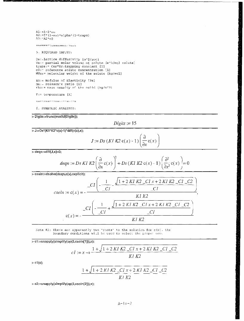
In the absence of body forces, this is a standard diffusion equation with a concentrationdependent diffusion coefficient. Solutions to the steady-state problem, with and without bodyforces, can be obtained straightforwardly by integration; symbolic computation isrecommended (see Appendix A).
Programming Simplifications
The following generalizations are made to the expressions for dilatational strain e andaxial stress Oa to simplify the subsequent finite element coding. They are obtained using Eqs.(19) and (20) and the definition for ACL:
e=Al U + A 2CL - A3 (22)ax-, = Ble - B2CL + B 3
where Ai and Bi (i = 1, 2, or 3) are constants defined in the table below:
Constant Plane Stress Plane Strain
A, (1 - 2u) 1
A2 2(1 + P)a,(1 + c'K2 ) 0
A3 A) x co 0
B1 3k (A + 2G)
B2 9ka,(1 + c`)•,) 3ka, (I + c'Kr)
B 3 B2x cQ B2 x cO
Table 1: Constants for the dilatational strain, c, and axial stress, ax, relations.
7

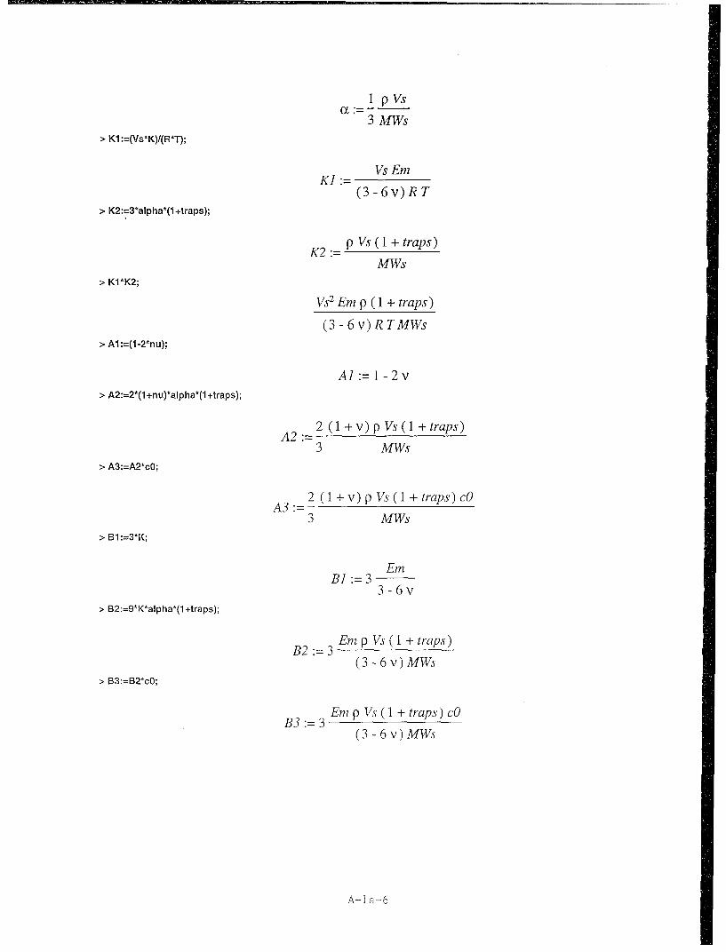
The elastic constants needed as input to the finite element program are the elasticmodulus, E, and Poisson's ratio, v. Conversions from bulk modulus, k, and A + 2G(A = Lam6 constant and G = shear modulus) are given by:
Ek-= (23)
3(1- 2v)A + 2G = (1 - u)E
(I + v)(1- 2v)
The equations of classical stress assisted diffusion result by setting the constants A2 , A3 , B2 ,and B3 equal to zero.
Formulation of the Finite Element Matrix Equations
Galerkin method of weighted residuals is used to formulate the finite element matrixequations. This procedure uses the interpolation functions as weights in the integralformulation given below [ 16]:
( L+ MJ )GidV= 0 (24)
OU± + Fx HI dVe 0
where: Gi ith' concentration interpolation function, (Gi Gi(x)).Hi ft displacement interpolation function, (H= Hj(x)).
dV- differential element volume = A6 dx.
A, -6 cross-sectional area (A. z Ae(x)).
Integrating the second term of Eq.(24a) and the first term of Eq.(24b) by partsyields the coupled set of equations for a single finite element of length h (0 < x < h):
h C Gj xj -JL {& i(x) A ,d ,7 i( )IIh ( 5_ X1 A, dx - A 6 5J; f (25)
- •' {& +) F• {Hj(x)})A~dx = - A•, {H5(x)} i
The RHS term AJL represents the axial solute influx through the element boundaries andAeu, represents the axial force applied at each end of the element.
Interpolation Functions for the Concentration and DisplacementThe concentration is represented using a linear interpolation function, and the
displacement is represented using a quadratic interpolation function:
8

2
CL Gi (x)ci(t) [LG(x)j{ci(t)} i 1,2 (26)i=1
0 x i=1 dx I_ dx I{j(t)} i= 1,2
DCL 2 dG i (t) dG ( t)jEEL3 = Gi(x)i~ /- Lai(x)j 7 i= 1,2at i=1 td
3
u- EHj(x)uj(t) LHj(x)j {uj(t)} j 1, 2,3 (27)j=1
Du 3 dH(j(x) dHj(x)
Ox E dx (t) dx j(t) jL=,2,3j=1
OU 3 duj(t) •u()
- EHj(x) Lyjx)J = 1, 2,3dt dat j=l
where L'"J indicates a row matrix and {...} a column matrix. Substitution of these intoEqs. (22a,b) and (17b) for the dilatational strain, stress, and mass flux, respectively, give:
e A1 d Hfx) {uj(t)} + A2 LGi(x)J{ci(t)} - A3 (28)crx •A d~ dx) 1!
=BIA, ~dIjjx) {uj(t)}+(BIA 2 - B 2) LGi(x)J{ci (t)} + (B 3 - B 1A3 )
Dc- D di(x) K, d {c((t)} ± Df D{(t) I
Substituting Eqs.(28a,b,c) into Eq.(25a,b) and collecting terms in {c(t)b}, {uM(t)}, {1(t) },and {zij(t)} yields the following matrix equation:
[[d E01 f I+ [KcI [K.] ] {c} {R}{ (29)101 101 f 7ijI[K. jI J 1
dc• 30where: {6I} d (30)
dui
dt
[Cc] - A, {fG(x)}I LG(x)j dx (31)
9

[K,] - [0] (32)[K] oh dHj(x) dHj(x)
[K _ Ae dx dx dx
[K.] = Ae j (BIA 2 - B 2 ){ dHj(x) } LGi(x)jdx
[ ]-dG(x) AdG((x1AK- ) Id[K] -Ae jhDeff({ dx dx K { dxdi(x)-ax LGi(x)J) dx
{R} -- Ae, J {Gj(x)} (33)
{!R•} - A, f ({Hj(x)}Fx - (B3 - B1A3) dHj(x) dx + Aex{Hj(x)} h• dx ýo • H()o
and where the cross-sectional area, Ae, is assumed to be constant within the element.The fact that [K0 ,] is zero might appear to imply that there is no coupling between
concentration and deformation, but this is not the case. The [K,] contains the first derivativeof the hydrostatic strain, ac/Ox, which contains, in turn, the second derivative in thedisplacement, u (from Eq. (22a)):
Oe 02u A2 OCL (34)OX 'ax-2 aX
The presence of the second order derivative in u would normally require the use ofC' continuous elements in order for u to satisfy element interface compatibility requirements[16]. To avoid this complication, the values of u and CL from the previous time step are usedto approximate ae/ax for the current time calculations.
The integral expressions in Eqs. (31)through(33) use interpolation functionsexpressed in terms of the global coordinate, x. The code will be implemented usingisoparametric coordinates 4 which requires replacement of the functions Gi(x) and Hj(x) byan appropriate set of isoparametric interpolation functions.
Isoparametric Interpolation Functions
Standard linear and quadratic isoparametric interpolation functions, expressed interms of the local coordinate r (- 1 < r < 1) are given by [17]:
11 '
gr) (1 r), 92() (1 +r) (35)2 2
hIii(r) (7 1( 2 _r), h12 () -(I - r2) h~3(r) (+ ( 2 + T')22
SThe transformation from global to local coordinates is isoparametric in displacement and superparametric inconcentration. The term isoparametric will be used here to refer to the local coordinate parametrization of theelement geoimetry which extends from -1 at the left-hand end of the element to +1 at the right-hand end.
10
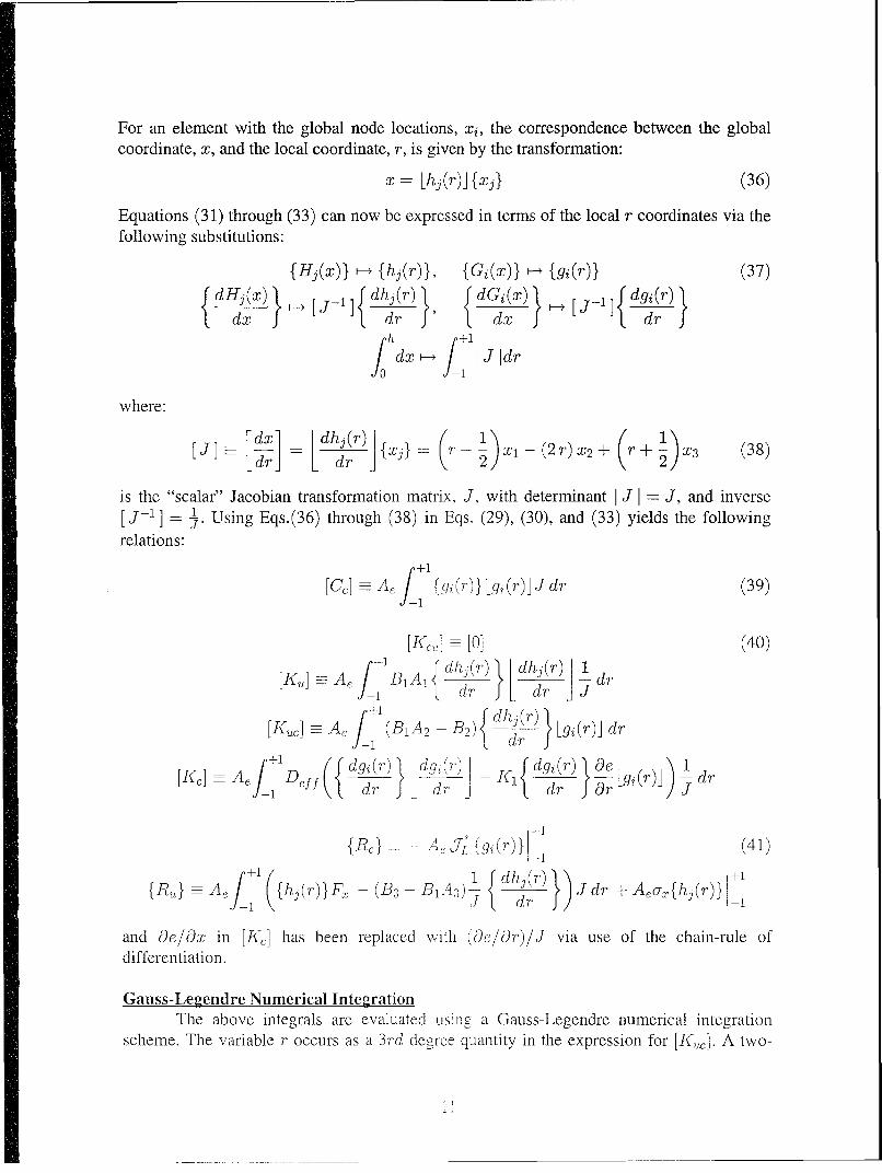
For an element with the global node locations, xi, the correspondence between the globalcoordinate, x, and the local coordinate, r, is given by the transformation:
x = [hj(r)J{xj} (36)
Equations (31) through (33) can now be expressed in terms of the local r coordinates via thefollowing substitutions:
{Hj(x)} -* {hi(r)}, {Gj(x)} F-+ {gi(r)} (37){dHj(x) ]{1 dhj(r) dGi(x) ]-[J- dgi (r)
dx dr dx drr
h +1jdx I* J 1dr
where:
]- = =Ldx dr -XjI r- x -(2r)X2+ r+ x, (38)
is the "scalar" Jacobian transformation matrix, J, with determinant J J, and inverse[J-l] = 1. Using Eqs.(36) through (38) in Eqs. (29), (30), and (33) yields the followingrelations:
[Cc] - A {gi(r)} Lg (r)J J dr (39)
[K,,1- [0] (40)
[K,]- Ae fB 1 A1 dhj(r) dhj(r) I - drfl-i dr' JL dr IJ J'
[K,,,]A, 1 A A~2 - B2) d r) Lgi(r)j dr-1 dr" ý
/+1 ({dgi (r`) dgi (r`) iKldgi(r) D e d1[K,]- A+f D~f f d r K rýO gl)
+r1
{Rc} A, 17 {gjQr)} (41)
[±l-Ae+ B3113 1 dhr)+1JR, A (I h- (B3 - l dh3 r Jdr +Acuzfhj(r)} E
and Oe/Ox in [K,] has been replaced with (Oe/&r)/J via use of the chain-rule ofdifferentiation.
Gauss-Legendre Numerical IntegrationThe above integrals are evaluated using a Gauss-Legendre numerical integration
scheme. The variable r occurs as a 3rd degree quantity in the expression for [IV,]. A two-
11

point integration using Gauss-point locations, rk + 1/V3, and Gauss weights, Wk = 1.0
is therefore selected for use in the numerical calculations [16,17]:
2
[Co-- L_,AeWk J(rk){gi(rk)} [gi (rk)J (42)k=1
[K,,] [0] (43)AWk BA1 { dhj(rk) dhj(rk)
[ -K J(rk) dr dr
[K.] - -Ae.Wk(BiA2 - B2) dr Lgi(N)Ik=1
[K,] E AWk Deff dgi(rk) dgi(rk) K, de i(rk)} Lgi(rk)Jk=1 J(rk) d'r dr
+1{R} =- Ae• {gi(r) -1 (44)
{fRlL•= AeWk J(rk)jhj(rk)}-(B3 - BA 3) dr) + Aec7x{hj(r)} _1k=1 dr
Finite Element EquationsThe matrix finite element equations given by Eq. (29) are rewritten, following
reference [16], in the form:
[C(vo)]{fi+}o + [K(vo) ]{v}0 = {R(to)} (45)
where {v} is the vector of nodal degrees of freedom and 0 (0 < 0 < 1) parameterizes thetime integration scheme via the following definitions:
to = t + OAt{v}o (1 - 0){v}f0 + O{V}f 1+ (46)
f {)10_ VIn"i - M"~At
For 0 = 0 and a lumped capacitance matrix, the algorithm is explicit; for 0 = 1, thealgorithm is Crank-Nicolson; for 0 - 2 the algorithm is Galerkin; and for 0 = 1, the
3algorithm is the backward difference.
The coupled temperature-displacement solver routine in ABAQUS is used to solvethe fully coupled system of transport equations represented by Eq. (45). This particularABAQUS routine uses the backward difference algorithm for time integration. Substituting0 = I into Eqs. (46) gives:
12

t8=1 = t.+1 = tn + At (47){1v}e=l1 {v}n+l
I i) 10=1 = I i) 1+l 1Vn+-- {v1}n
At
which, when substituted into Eq.(45) yields:
[[K(v+)] [C(vn+l)] vn+l-AA {V} -- {IR(tn+i)} (48)
If [C] and [/C] are independent of the degrees of freedom {v}, then the problem is linear, andthe equations may be solved directly for {v} 1+, via standard linear systems solver routines.On the other hand, if [C] or [1C] is a function of v, then Eq. (48) is non-linear and must besolved using more specialized techniques. One of the techniques used by ABAQUS is theNewton-Raphson method. It is described below.
Non-Linear Solutions via Newton-RaphsonAssume that {v}j, is known and we wish to determine {v},+1 . First, define the
"residual" vector {f (vn+±)}:
{f(vn+l)} +- AP+A] t 01 -){v}n+l (49)
[C(v+i )1)- /At {t }-{R-(tn+l)}
where {f(v,+l)} = {0} for a {v} n+ which is a solution to Eq. (48). Defining {v}n'l as the
ith iterated approximation to the actual solution, {v} n+, leads to the following definition for
the (i + 1)"t iterated approximation:{v}ij3 {} + {Av}i+ (50)
i+1 A i+1
where jAvj'+ 1 is a correction vector. This correction vector {Avjn+1 can be determined byexpanding {f(v±+l)} in a Taylor's series approximation about the point {v}l'+l, retainingonly the zeroth and first order terms, and then setting the resulting expression equal to zero:
{f(v'i+1 ) (vn+1)} + a{f(vi+I)} {Av}• + '1 {} (51)
0 f (Vi(n+1l)I
Now, {V1 _ [K + [Civ- 1 I (52)+ At
-) [C'(+ 1 )] 3[C"(v+ ]
13
where we have defined:
n+1 1 {V})+1 (53)
1K,~ [&[KI Ovji IVIn1n{}+1
[e,,(<+• r _= [C(v÷ )]1{(+ [ [c'
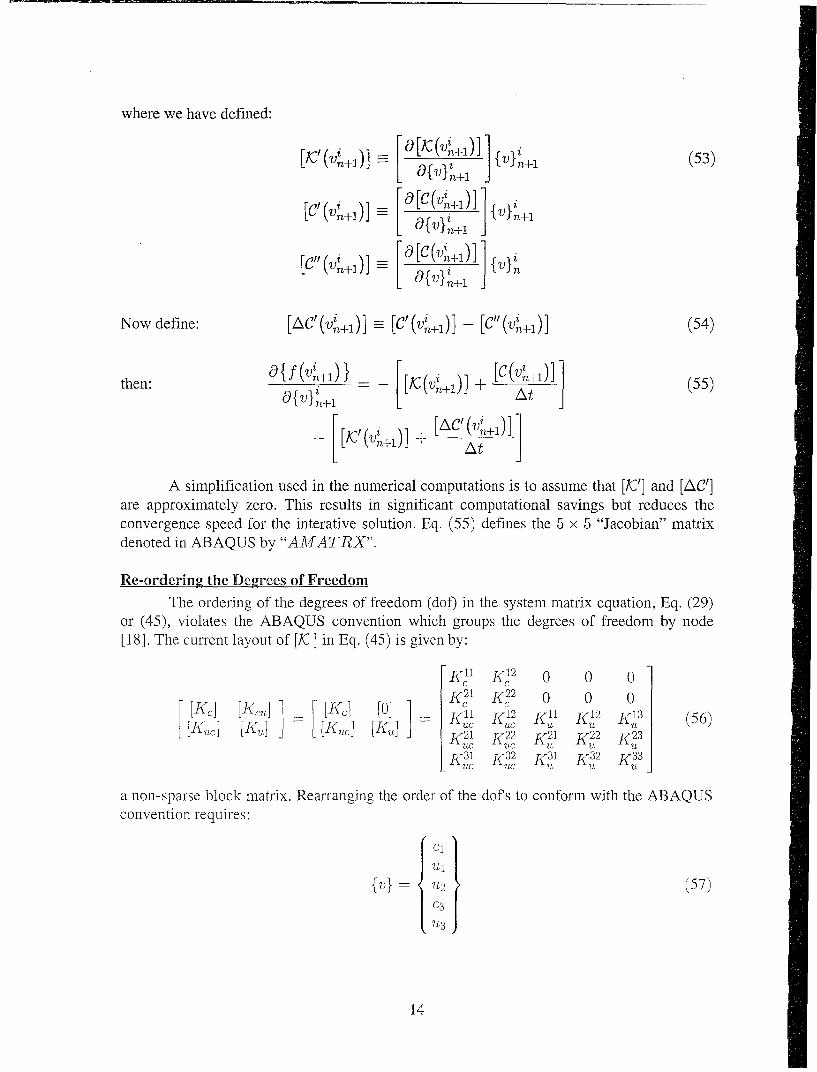
A simplification used in the numerical computations is to assume that [/I7'] and [AC']are approximately zero. This results in significant computational savings but reduces the
convergence speed for the interative solution. Eq. (55) defines the 5 x 5 "Jacobian" matrixdenoted in ABAQUS by "A MATtRX".-
Re-ordering the Degrees of Freedom
The ordering of the degrees of freedom (do) in the system matrix equation, Eq. (29)
or (45), violates the ABAQUS convention which groups the degrees of freedom by node[181. The current layout of [(C] in Eq. (45) is given by.
=[Ki K K• K,• K[2 K(V3 (56)
[hen: LUJj '+j I~ +~ KAt K 2
a non-sparse block matrix. Rearranging the order of the dofs to conform with the ABAQUS
convention requires:
14

This reordering gives the new element stiffness matrix layout:K1' 0 0 Ki 2 0
K 11 K11 K12 K12 K13[ KE] K2 KU21 K22 K 22 K2 (58)
K,21 0 0 KC2 0
The capacitance matrix must also be altered to reflect the new ordering given by Eq. (57).
ABAOUS User Element Subroutines
ABAQUS executes a Fortran subroutine named UEL for each "user defined" finiteelement in the model. Current values for the: 1. material properties; 2. total and incrementalnodal degrees of freedom; 3. time incrementation parameters; and 4. user-defined statevariables (i.e., the dilatational strain and axial stress at the Gauss integration points;extrapolated axial stress at the element boundaries; the mass flux at the center of the element;and the Gauss point locations) are passed from the main ABAQUS code into the UEL.Depending on the exact stage in the time increment, the subroutine UEL must return somecombination of the: "Jacobian" matrix (AMATRX); right-hand side vector (RHS); andupdated values of the state variables.
From Eq.(5 1), we have:a If (vi+ - {If (V +l)} (59)
n I ^ fvinl
or AMATRX { Avl+'= - RHS (60)
1
where AMATRX,• 1 [C(vin+)] + [±(Vn+l)] (61)At
and RHS = {ýR} - [iC]{ [C{Av}+ (62)
On return from subroutine UEL, ABAQUS assembles the AMATRX and RHSfrom each element into the global matrix equation:
[AMATRX]M{Av}K+11 {RHS}G (63)
and adds contributions from concentrated loads into the RHS array. ABAQUS solves Eq.(63) for the incremental correction {Avy+1 using standard solution techniques. The solutionprocess is repeated until the residual, that is, the {RHS}G vector, is smaller than somespecified tolerance, at which point the solution is accepted as correct. The tolerances usedwith this UEL subroutine must typically be set in the ABAQUS input deck, since theresiduals for the displacement and concentration variables generally show many orders ofmagnitude difference.
15

MODELING APPLICATIONSA variety of one-dimensional hydrogen transport problems have been used to explore
the differences between the fully coupled transport theory, described in this paper, andclassical SAD theory. Analytical and finite element solutions for the steady-state distributionsof: hydrogen, axial stress, axial and dilatational strains, and the axial displacement have beenobtained for a (10 cm x 1.0 cm 2) cylindrical rod of 4340 steel subjected to various boundaryconditions and applied body forces. Plane stress conditions are assumed for all problems.
The boundary conditions consist of concentration or mass flux and displacement orload (stresses) at each end of the rod. The analytical solutions are obtained using the Maplesymbolic computation program, and the numerical solutions are obtained using ABAQUSwith our custom Fortran user element subroutine. The problems examined both analyticallyand numerically are summarized in Table 2. Other problems that have been examinedanalytically are documented in Appendix A.
Case # Deformation Boundary Conditions Diffusion Boundary Conditions Body Force # Elementsla u(LHS) = 0.0 P (RHS) 0.0 cL(LHS) = 0.0 CL(RHS) = 10-1 0 102a u(LHS) = 0.0 u(RHS) = 0.0 cL(LHS) = 0.0 CL(RHS) = 10-6 0 10
3 (LT) u(LHS) =0.0 PJ.,(RHS) 0.0 7L(LHS) =0.0 CL(RHS) = 10' 15)<106 200
3 (HT) u(LHS) = 0.0 PX(RHS) 0.0 JL(LHS) = 0.0 CL(RHS) = 10-7 15X106V' 200
Table 2: Displacements, u, are specified in [m]; loads, P•, in [N]; concentrations, CL, in[gH/gFe]; mass flux, JL, in [m/s]; and body force, Fx, in [N/r 3 ]. Case 3a (LT)and (HT) correspond to low and high trapping (1 + clKR = 20 and 500).
Case 1 and 2 problems were used to gain insight into the differences between the fullycoupled theory, SAD theory, and classical diffusion theory. They also proved useful asbenchmark problems for debugging and verifying the user element subroutine.
Case 3 was posed in order to better assess the influence of the hydrogen induceddeformations, which are not accounted for in classical SAD theory, at a crack-like stresssingularity. A square-root singular stress was introduced in the rod by subjecting it to thefictitious body force:
15 x 106 (64)VI(I - (64
The variable e is a small constant (2.0 x 1 0 -1S) included to prevent inadvertent Fortranerrors at x = 0. Substituting this into Eq. (18) and integrating results in the square-rootsingular stress:
30 x 106(65)
The numerator of Eq. (65) is equivalent to a stress-field intensity factor, K, which means thatwe have adopted a stress-field K value of 30 [MPa/in] for these Case 3 problems.
The introduction of this singularity into the 1-D rod problem resulted in someinteresting, but unexpected, behavior in the mathematical solution for the concentration as a
16

function of x. We found that the concentration becomes a multi-valued function of x as thesingularity at x = 0 is approached. The exact point at which the concentration becomesmulti-valued is predictable and depends only on material constants. Various features of theanalytical solution will be discussed in the following Results and Discussion sections, but asa consequence, we have had to modify the rod geometry in our Case 3 numerical analysis sothat the left hand boundary starts at x = 4.0 x 10⁻⁵[m] rather than x = 0. This avoids thenumerical problems associated with multi-valued concentrations.
The material properties used in the analytical and numerical analyses are given belowin Table 3:
Property ValueMass Density, p 7.8 [g/cm 3]Temperature, T 293 [K]
Lattice Diffusion Coefficient1 , DL 1 x 10⁻⁵ [cm 2/s]
Partial Molar Volume of Hydrogen 2, VH 2.0 [cm 3r/mol]Saturation Trapping Concentration 3, cR 2 x 10¹² to 10-' [g H/g Fe]Reversible Trap Binding Enthalpy3 , HB 3.3 to 30 [kJ/mol]
KR = exp(-T) 4 to 2.2 x 10⁵
Trapping Factor, (1 + c'KR) 20 and 500Molecular Weight of Hydrogen, .ML 1.00797 [g/mol]
Modulus of Elasticity, E 200 [Gpa]Poisson's Ratio, v 0.3
Reference Concentration, co 0 [g H/g Fe]
Table 3: Material property values used in the Maple and finite element analyses.
RESULTSThe results are presented in two subsections. The first subsection corresponds with
the Case la and 2a problems, and the second subsection corresponds with the Case 3problem. Each subsection is further divided into parts describing the analytical and finiteelement solution procedures and description of results.
Case 1 & 2 ProblemsAnalytical solutions to the 1-D problem can be obtained by solving Eq. (21) for
concentration. For the convenience of the reader, Eq. (21) is repeated below:
OCL =9 0l V, f; 1 I sKR CL +V, Def fFCL (1OCt O [Df i MLRT(1-c•KR)CL)± +3{fFxcL (21)
I Approximate value taken for a-Fe from Figure 12.4 of reference [19].2 Approximate value taken from Section III.A.2 of reference [6].
3 Range of values obtained from Table I of Section III.B. I of reference [6] with HB < 30 [kJ/mol].
17

This is a non-linear diffusion equation with a concentration dependent diffusion coefficient.Under steady state conditions the equation simplifies to:
( + c' KR ) dcL +Vs FCL = Constant (66)1 A4LRT i •R )c ---x 31R--T
where the constant is proportional to the mass flux that obtains under steady-state conditions.For Cases 1 & 2, the body force, Fz, is also taken to be equal to zero, so that the
governing differential equation simplifies to:
(I M=c'TKR) d Constant (67)pV(1k R ) d-L
This equation can be integrated to give cL(x), and once CL(x) is known, Eq. (18) and (22b)can be combined to give:
de _ B 2 dCL(X) (68)dx B1 dx
This can be integrated using the known function cL(x) to give the dilatational strain, e, andthe axial strain and axial stress can then be obtained directly from Eqs. (22a,b):
du _ e(x) _ A 2 A 3dx A1 A, A(
rx = Bie(x) - B2CL(X) + B 3
Finally, the displacement, u, can be obtained by integrating Eq. (69a). The constants ofintegration in the expressions for: CL(x), JL, e(x), cx(x), g,(x), and u(x) can be determinedusing the given boundary data.
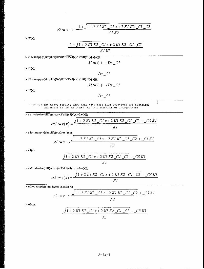
The above steps were performed, in this work, using the Maple V symboliccomputation program on a Sun SPARC1O workstation. The general results are given below:
CLW = CX + C I - C 2X (70)
U(x)=C 3 x+(C 4 -C 5 X)!1- C2 x-C 4 (71)
(x) = C6 - C 7 \ - C 2X (72)
-7 Cs (73)
JL = C9 (74)
where the Q, i c {1, ... , 9} are constants that depend on the boundary conditions andmaterial property values. Documentation of the Maple analyses is given in Appendix A.
18

For the ABAQUS finite element analyses, the 10 [cm] rod is discretized using tenelements of length 1 [cm]. The initial concentration and displacement are specified as zerothroughout the rod, and the boundary conditions are as indicated in Table 2, and in thefigures below. A "coupled temperature-displacement; steady-state" ABAQUS analysis isperformed with an initial time increment of 5 x 10⁻³ [s], a total step time of 1.0 [s], and amaximum allowable increment of 0.5 [s]. The residual magnitude for the concentration dof issignificantly smaller than the residual for displacement dof. A separate convergence criterionfor the concentration (temperature in ABAQUS) dof is therefore adopted. The initial time-average flux for convergence of the concentration dof is set at 5.0 x 10⁻²¹ (see the AUM[II;9.6.2-1]). The input decks for the Case la and 2a analyses are given in Appendix C.
Case la and 2a rod geometries and boundary conditions are shown in Figures 3 and 4.Figures 5 through 11 show plots of: CL (X); the difference between the linear concentrationdistribution that obtains from classical SAD and diffusion analysis and cL(x); e(x); u(x);and orx(x). Keep in mind while examining these plots that e(x), cx(x), u(x), and o-x(x) areidentically zero for the classical SAD or diffusion analyses.
10 CM 10 CMA=1 cm2 A=] cm 2
CL(O) =0 CL(O. 10)l -6 CL(O)O cL(O.I O)=O -6u(o) =0 o(o0o10)=o u(O)=0 u(0.J0)=O
Figure 3: The rod geometry and boundary Figure 4: The rod geometry and boundaryconditions for Case la. conditions for Case 2a.
1 .0 6.010-
0.8 - ABAQUSAnalytical
0.6
0.4 0
2.0
o 0.2
U
0.0 0.0'0 2 4 6 8 10 0 2 4 6 8 10
Distance, x [cm] Distance, x [cm]
Figure 5: Analytical and finite element Figure 6: Difference between classicalconcentration predictions for Cases la diffusion or SAD and the fully coupledand 2a using the fully coupled theory. concentrations (i.e., 10- 7 x - CL(X) ).
Figures 5 and 6 show the concentration and concentration difference, which areidentical for the Case la and 2a problems, as a function of position along the rod. Theconcentration difference is defined as: 10-7x - CL(X) where 10-7X is the concentrationdistribution that obtains for the SAD and classical diffusion theories. The difference ismaximum at the center of the rod, but is very small at • 5.5 parts per billion (ppb). Thedifference between the analytical and finite element predictions is less than 0.05 ppb.
19

0.6:,0.3 " ABAQUS T /S-- Analytical l sAB QU
X ABAQUSW 0.4 Analytical= 0.2 x
0.1o E 0.2Cd
0.0 0.0
0.0 2.0 4.0 6.0 8.0 10.0 0 2 4 6 8 10
Distance, x [cm] Distance, x [cml
Figure 7: Fully coupled dilatational strain Figure 8: Fully coupled displacementprediction for Case la. The FE predictions prediction for Case la. The FE predictionsare given at Gauss integration points, are given at the nodes.
Figures 7 and 8 show the dilatational strain and the axial displacement experienced bythe rod for the case la conditions. The rod is traction free, and there are no applied bodyforces, so by Eq. (18), the stress in the rod must be zero. By way of verification, we note thatthe FE analysis (not shown) also predicted a zero stress throughout the rod. The maximumdilatational strain and axial displacement occur at the free end of the rod with magnitudes of; 310 [/um/m] and ; 5.2[/,m] respectively.
0.000.3 - ABAQUS
a. ABAQUSX 02, -0.04 Analytical
0.2
- -0.08- 0.1 C
Ca aa -0.12
0.0 2.0 4.0 6.0 8.0 10.0 0 2 4 6 8 10
Distance, x [cm] Distance, x [cm]
Figure 9: Fully coupled dilatational strain Figure 10: Fully coupled displacementprediction for Case 2a. The FE predictions prediction for Case 2a. The FE predictionsare given at the Gauss integration points, are given at the nodes.
Figures 9 and 10 show the dilatational strain and axial displacement for Case 2a. Therod, stress free in the absence of hydrogen, tries to expand when the hydrogen is introduced.A uniform axial compressive stress of : 10.4 [Ivf Pa] (see Figure 11) is introduced becauseof the zero displacement boundary restraints at the walls. The dilatational strain is positiveand maximum at the RH boundary of the rod, and small, but negative at the LH boundary.The axial displacement is negative throughout the rod indicating a leftward movement of therod material. The maximum displacement of z - 1.3 [t.nm] occurs at the center of the rod.Recalling the definition of axial strain, , = du/dx, we see that it is negative in the left halfof the bar, positive in the right half, and zero in the middle. The maximum strain ( ± 50[fu]) occurs at each end of the rod (see the figure on page A-2a-14 of Appendix A).
20

0.0
(a1
S-5.0 * ABAQUS- Analytical
S-10.0
-15.00.0 2.0 4.0 6.0 8.0 10.0
Distance, x [cm]
Figure 11: Fully coupled axial stress prediction for Case 2a. The FE predictionsare given at the Gauss integration points.
Case 3 ProblemsThe governing differential equation for the Case 3 problem is obtained from Eq. (66)
by substituting in for the applied body force, Fx:
( (I+2cKR)CL dcL V,(15x 10')1 ML IRT 1) - 3RT CL =Constant (75)
Analytical solutions to this equation are obviously more difficult to obtain than in theprevious two cases.
The LHS of Eq. (75) is directly proportional to the mass flux JL; the mass flux istherefore constant throughout the rod. The Case 3 problem under study imposes a zero massflux boundary condition on the LH boundary. The constant in Eq. (75) can therefore be setequal to zero, leading to the following governing equation:
(I k( 1 + C' KR)CL dCL v (15 x 10L6)LLRT - 3 / (76)
This must be solved for CL as a function of x (i.e., for CL(X)).An interesting observation regarding Eq. (76) can be made. As CL(X) increases from
some vanishingly small value, the coefficient of the derivative term will go from positive tonegative, passing through zero on the way. When the coefficient equals zero, the derivativeterm drops out and we are left with the equation:
V8 (15 X 10L6)
3 R T 7x 3
This equation cannot be satisfied because CL is not zero, x is finite-valued, and the rest of thevariables are either non-zero constants or material properties. A mathematical solution to theproblem can only be obtained by letting dcL/dx -- z: as:
21

,LX)A4LRT (78)CLI~X) --' -2p Vs k(1+ KR)
Allowing this results in multi-valued concentration solutions to Eq. (76); Eq. (78) defines thepoint at which the solution becomes multi-valued. Since multi-valued concentrations are notphysically realistic, the assumptions made in the derivation of the fully coupled transportequations must be re-examined. This is done in the following Discussion section.
The solution to Eq. (76) is obtained by integration using Maple (see Appendix A):
eL(X) = -- C10w CIO (79)
W(x) is Lambert's W function 4 , and the Ci, i C {10, 11, 12} are constants related to thematerial properties and boundary conditions. This equation is multi-valued in x, but it can beinverted to give x as a single-valued function of eL:
X(CL) (C12)2 (80)01-0 -- in(CL)- C11
The stress field is obtained by integrating Eq. (18) with the applied body forcesubstituted in for Fz, yielding:
30 x 106ax(X)= V/•(81)
The dilatational strain can be written in terms of a, and CL using Eq. (22b):
e (X) =_ 1(GuX(x) + B2 CL (X) - B 3 ) (82)B1
Similar operations can be performed on Eq. (22a) to determine du/dx which can then beintegrated (analytical integration may not be possible) to obtain the displacement, u(x).
The ABAQUS analysis for Case 3 requires significantly smaller elements than theCase 1 and 2 analyses, particularly near the singularity. The rod is discretized into 200elements of length 1i = 0.104/0.94i-1 [trn] where the first and smallest element, 11 = 0.104[trm], is placed at the left hand end of the bar, x = 4 x 10- 3 [cm]. The 0.94 factor in thedenominator is known as the element "bias" in ABAQUS. A "coupled temperature-displacement; steady-state" analysis is used with an initial time increment of 1.0 x 10- 4 [s],a total time of 1.0 [s], and a maximum time increment of 5.0 x 10⁻³ [s]. The initialdisplacements in the rod are taken as zero, but an initial uniform concentration equal to theRH boundary concentration of 1 x 10⁻⁷ [g H/g Fe] is assumed. To match this initialcondition in the analysis, the RH boundary concentration is applied as a step rather than a
4 Lambert's W function satisfies the equation: W(x) x exp (W(x)) = x. Additional information can be foundusing the interactive Maple V help program.
22

ramp function. Providing an initial concentration resulted in a more rapid convergence of thesolution to the steady-state values. The residual magnitude for the concentration dof issignificantly smaller than the residual for displacement dof. A separate convergence criteriafor the concentration (temperature in ABAQUS) dof was therefore adopted. The startingtime-average flux for convergence of the concentration dof is set at 5.0 x 10⁻²¹ (see theAUM [II;9.6.2-1]). The input deck for the Case 3 analysis is given in Appendix C.
The Case 3 rod geometry and boundary conditions are shown in Figure 12. Figures 13through 17 show: cL(x); ln(cL(X)) - constant which illustrates the different concentrationsingularities; e(x); u(x); and ax(x). Plots are given for the fully coupled theory under lowand high trapping conditions, for SAD theory, and in many cases, for Fx 0. The finiteelement results are plotted for every 20th element.
Body Force, F.15 X 106 -- S.A.D.
F, 32[N/rn 3] 5.0 -- SD
"F 4NI- 5.0 • 5AnalyticalC 4.0l 500 F.E.M.X
3.0X x[m] 2 2.0 Q,
40cmI- 10 cm "62.
A=] cm 2ow Fý= 0...
11.0 1JL(4.0 X 10 -5)=0 cL(0.10)=l0 -7 10-3 10-2 10-1 100
u(4.0 x 10 -5) =0 GX(O. 10) =0 Distance, x [cm]
Figure 12: The rod geometry, boundary Figure 13: Concentration predictions forconditions, and applied body force for the Case 3. The SAD results lie under the LTCase 3 problem. (20) curve of the fully coupled theory.
C 10.0 5 Analytical
500 220
20/ "~i 1.0 0.78
0.1
S.A.D. 0.12
- Analytical101 " • F.E.M. 0.031 - --- '--e - - - ------
0.0 110-3 10-2 10-1 10( 10-3 10-2 10-1 100 101
Distance, x [cm] Distance, x [cm]
Figure 14: Concentration singularities. Figure 15: Dilatational strain for Case 3The SAD & LT-20 curves are coincident, using the fully coupled and SAD theories.
Figures 13 and 14 show the predicted concentrations for the Case 3 problems usingfully coupled and SAD theories. The SAD predictions are made using the classic expression:
CLW =c CXP(V, I 30X- 10) (83)
23

The fully coupled model predicts slightly larger concentrations than the SAD model, withincreasing differences as the singularity is approached and as the degree of trappingincreases. Figure 14 shows that the singularity for the fully coupled concentration is moresevere than the exp (I/Jf) singularity of the SAD model, at least for the high trapping case.
10.0 10,- Fully Coupled w/ F.
,S 8.0 FullyCoupledw/oF. 2.48-0.50log()C OUncoupled with F. 500 2 5
S6.0
"I • • 103S4.0S+
. 2.0 .-
0. ý 101 ,-0 2 4 6 8 10 10-3 10-2 10-1 100 10'
Distance, x [cm] Distance, x [cm]
Figure 16: Nodal displacement curves for Figure 17: Gauss point stresses with athe FE analysis of Case 3 for the fully least squares line fit showing the requiredcoupled and SAD theories, straight line behavior with a - 1/2 slope.
Figures 15 and 16 illustrate the dilatational strains and nodal displacement curves. Aswith Cases 1 and 2, the fully coupled model predicts larger displacements and dilatationalstrains throughout the rod. Again, the difference between the fully coupled and SAD modelpredictions increase with the degree of trapping. The zero-body force strains anddisplacements are also shown for comparison with the zero valued strains and displacementsthat obtain for the SAD and classical diffusion model. Figure 17 shows the FE calculatedGauss point stresses; these match the expected behavior.
DISCUSSIONThe above three rod problems illustrate the differences between the fully coupled and
classical SAD theory under steady-state conditions (additional results can be found inAppendix A). The results show that the concentration differences are generally small, butgrow in the region very near to the singularity. The deformation differences are a bit morepronounced, especially in Cases 1 and 2 where the boundary and body force loadings areabsent. All of the fully coupled results are dependent on the degree of trapping.
The results also showed that accurate finite element solutions are possible for thefully coupled transport theory using ABAQUS with custom user element subroutines. Theexperience gained during the development and application of this 1 -D user element routine isproving to be very useful in the ongoing development of the 2-D user element subroutine.
The dependence of the concentration and deformation distributions on the trappedhydrogen may be useful in the development of new "Gorsky effect" experiments for trappingcharacterization. Perhaps the time dependent displacement at the free end of a cantileveredrod can be related to some transport or trapping parameter of interest. Transient Case 1 typeproblems are probably be most useful in this regard.
24

Regarding the multi-valued concentrations that appear in the mathematical analysis ofthe Case 3 problem, the values of CL satisfying Eq. (78) for the 4340 steel considered are:2.3 x 10⁻⁵ and 9.3 x 10⁻⁷ [g H/g Fe] for the low (LT) and high (HT) trapping conditions,respectively. The total internal hydrogen, in mass fraction concentration units5, is given byEq. (6): ctotal - 4.7 x 10⁻⁴ + c' [gH/gFe]. Now, this is a very large concentrationcompared with the solubility of hydrogen in pure iron at room temperature and 1 [atm]pressure (Ctotal - 2 x 10-' [gH/gFe] or 1 x IO7 [H/Fe]). It leads us to question theassumptions made regarding the magnitude of the concentration in the development of thefully coupled model. The three major assumptions include: 1.) "infinite" dilution of the totalhydrogen in the mixture; 2.) ideal behavior; and 3.) material properties that are independentof the hydrogen concentration level.
The magnitude of the lattice concentrations at the critical point are still much lessthan one. It is unlikely, therefore, that the assumption of infinite dilution is playing any rolein this particular situation. Extension of the model to include finite concentrations, while stillretaining the ideal solution assumption, can be made by adopting a "reduced" chemicalpotential [15], which takes into account the blocking of interstitial sites in the neighborhoodof a hydrogen atom 6 . Reduced chemical potentials will be adopted in a future version of thetheory assuming that the multi-valued solutions for the concentration can be eliminated.
If we maintain the infinite dilution assumption, then non-ideality cannot play a rolebecause an infinitely dilute mixture is by definition, ideal. Non-ideal effects are only possiblein finite dilution mixtures [15], and the use of non-ideal expressions in classical SADmodeling is almost non-existent. Kirchheim and Hirth [20] have proposed a first orderextension which accounts for H-H interactions. The work by Fukai [21] and coworkers onpredicting hydrogen solubility in metals under very high pressures may also be of use inextending our model to include non-ideal effects. The question still remains; will theadoption of a non-ideal chemical potential result in governing equations with single-valuedconcentrations? We do not presently have an answer for this question; it remains to beinvestigated in the future.
The last possibility involves the assumption of constant valued material parameters. Ifthe RHS of Eq. (78) were to increase at least linearly with CL, through some concentrationdependence of the material parameters, then the multi-valued solutions will not occur. Alinear decrease in p, or k, or a square-root decrease in Vs, with increasing CL levels wouldsatisfy this requirement. Experimental evidence for these decreases in 4340 steel do notappear to be available in the literature. There is evidence, though, for decreases in V, at largeCL values for various other alloys (see, for example, the article by Peisl in [19; pp. 53-74]; orFukai [21; pp. 95-100]. This possibility will also have to be investigated in the future.
There remains one final aspect of this multi-valued solution dilemma that needs to bediscussed. That is the validity of square-root stress singularities in the fully coupled theory.Remember that this singular body force was artificially introduced in order to get the square-root singular stress. We have not yet determined whether square-root singular stresses willnaturally occur at the tip of a crack in the fully coupled theory. The 2-D finite element modelunder development should shed some light on this issue.
5 Multiplication of ctota! by AMFC/MAI ! 55 gives the mole fraction concentration, xtotai = 2.6 x 10⁻² + 55 cs6 Reduced chemical potentials are also referred to as the "Fermi-Dirac" potentials [20-22].
25

SUMMARY AND FUTURE RESEARCHThe focus of this research was on the development of a finite element code for
coupled hydrogen transport and trapping in linear elastic metals for use in modeling hydrogenassisted cracking processes. A fully coupled solute transport model was developed; a 1-Dversion of the model was implemented in a finite element code via a custom Fortran "userelement" subroutine for use with the ABAQUS finite element program. A series of threesimple 1-D problems were posed to develop an understanding of the fully coupled transporttheory, and for verifying the accuracy and coding of the l-D user element subroutine. Steady-state solutions for the fully coupled theory, and for classical diffusion and stress-assisteddiffusion theories, were obtained analytically and numerically using the Maple symboliccomputation program and ABAQUS. Differences in the predicted concentrations anddeformations between the various theories were observed.
One of the problems incorporated a square-root singular stress as a "l-D analog" ofthe hydrogen transport problem in planar crack geometries. The fully coupled predictionsshowed slightly higher hydrogen concentrations, a more severe singularity in theconcentration, larger axial and dilatational strains, and larger axial displacements, all ofwhich depended on the extent of hydrogen trapping. The results indicated that the hydrogeninduced deformations, present only in the fully coupled theory, were more influential withregard to the displacements and strains.
Development of a 2-D user element subroutine is ongoing. The initial versions will belimited in scope to simple linear elastic mixture behavior and equilibrium trapping atreversible and irreversible trap sites. Rectilinear isoparametric 8-node displacementl4-nodeconcentration interpolation functions will be adopted. Extensions of the model to includenon-equilibrium trapping effects and plastic crack tip deformations are planned. An effort isalso being made to interface the ABAQUS code with our user element routines to the PatranSolid Geometry Modeling program. This will provide us with a convenient means ofmeshing complex 2-D geometries and manipulating and displaying the finite element results.
After the 2-D code has been developed, it will be used to calculate deformations andconcentrations in the crack tip region of a metal with uniform hydrogen concentrationsimposed along the crack walls. Steady-state SAD solutions for this idealized problem areavailable for comparison. The results will provide definitive answers on the importance ofthe hydrogen induced deformations in crack tip modeling.
A longer term goal is the use of the 2-D code to help establish an energy-basedparameter that characterizes the driving force for crack growth in the presence of adeleterious environment. This parameter, the.free energy release rate F, will generalize theclassical strain energy release rate g to include the hydrogen induced deformation energy andthe "free" chemical energy. It is defined by:
A(Externally Supplied Work - Specific Free Energy of the Hydrogen-Metal Mixture)A(Crack Length)
The use of F as a driving force for crack growth in environmentally assisted crackingappears to be a novel extension of the classical fracture mechanics concept. The advantage ofF over the stress intensity factor K (or AK) approach will be its ability to account forloading, environment, and material effects on the driving force for crack growth in terms of asingle variable. The concept will be applicable many material-environment crack systems of
26

technological interest including: hydrogen assisted cracking of metals, high temperatureoxidation cracking of superalloys, and moisture induced cracking of organic composites.
The magnitude of F in any environmental cracking situation will have to bedetermined by an analysis of the deformation and diffusion/trapping processes operative inthe crack tip region. More specifically, the deformation state (stresses and strains) andchemical state (potentials and concentrations for each solute species) of the mixture will haveto be determined as a function of the loading (e.g., a or Au, R, f, waveform, etc.),environment (e.g., phase, species, concentrations, T, pH, potentials, partial pressures, etc.)and material (e.g., elastic moduli, trapping parameters, solubility, diffusion coefficient, etc.)parameters. This information will be obtained using: a.) the fully coupled theory to model thedeformation-diffusion-trapping processes occurring in the crack tip region (governingequations); b.) an experimentally determined distribution of absorbed species along the crackwalls (boundary conditions); and c.) a method for solving the resulting mathematicalequations (the FE code).
Our initial efforts will be focused on the application of this concept to hydrogenassisted cracking of high strength metals. This system is ideal in the sense that it shows largeenvironmental effects, is important in many applications, and is supported by an extensivedata base. It also avoids the complications of large scale crack tip plasticity. Validation of theconcept will require demonstration of a unique correlation between the crack growth rate and.F (or A.F) for a variety of materials subject to a variety of loading, environment, andmaterial conditions.
ACKNOWLEDGMENTSThe first author's discussions with Dr. Peter Matic of the Naval Research Laboratory
concerning various aspects of the theoretical model, and both author's discussions with Dr.David Kirkner of the University of Notre Dame concerning the finite element modeling aregratefully acknowledged. The support of this work by Dr. John Sedriks of the Office of NavalResearch under Grant No. N00014-93-1-0845 is also gratefully acknowledged.
27

REFERENCES1. J. C. M. Li, R. A. Oriani, and L. S. Darken, (1966), "The Thermodynamics of Stressed
Solids", Z. Physik. Chem., Vol. 49, pp. 271-290.2. H. W. Lui, (1970), "Stress Corrosion Cracking and the Interaction Between Crack-Tip
Stress Fields and Solute Atoms", Trans. ASME-J. Basic Engng., Vol. 92, pp. 633-638.
3. P. Sofronis, and R. M. McMeeking, (1989), "Numerical Analysis of Hydrogen TransportNear a Blunting Crack Tip", J. Mech. Phys. Solids, Vol. 37, pp. 317-350.
4. H. K. Birnbaum, (1990), "Mechanisms of Hydrogen-Related Fracture of Metals", inEnvironment-Induced Cracking of Metals, Gangloff, R. P., and M. B. Ives, Eds., NACE-10, National Association of Corrosion Engineers, Houston, TX.
5. Hydrogen Degradation of Ferrous Alloys, (1985), R. A. Oriani, J. P. Hirth, and M.Smialowski, Eds., Noyes Publications, Park Ridge, NJ.
6. J. P. Hirth, (1980), "Effects of Hydrogen on the Properties of Iron and Steel", Metall.Trans. A, Vol. 11A, pp. 861-890.
7. R. N. Iyer and H. W. Pickering, (1990), Annu. Rev. Mater. Sci., Vol. 20, pp. 299-338.8. A. Turnbull, (1982), "Review of the Electrochemical Conditions in Cracks with
Particular Reference to Corrosion Fatigue of Structural Steels in Sea Water", Reviews inCoatings and Corrosion, Vol. 5, pp. 43-171.
9. T. R. Beck, (1977), "Techniques for Studying Initial Film Formation on Newly GeneratedSurfaces of Passive Metals", in Electrochemical Techniques in Corrosion, R. Baboian,Nat. Assoc. of Corrosion Engineers, Houston, TX, pp. 27-34.
10. Newman, R. C., (1984), "Measurement and Interpretation of Electrochemical Kinetics onBare Metal Surfaces" in Corrosion Chemistry Within Pits, Crevices, and Cracks, A.Turnbull, Ed., Her Majesty's Stationery Office, London, UK, pp. 317-356.
11. A. McNabb and P. K. Foster, (1963), "A New Analysis of the Diffusion of Hydrogen inIron and Ferritic Steels", Trans. TMS-AIME, Vol. 227, pp. 618-627.
12. B. G. Pound, (1989), "The Application of a Diffusion/Trapping Model for HydrogenIngress in High-Strength Alloys", CORROSION, Vol. 45, pp. 18-25.
13. H. H. Johnson, (1988), "Hydrogen in Iron", Metall. Trans. A, Vol. 19A, pp. 2371-2387.14. R. Oriani, (1970), "The Diffusion and Trapping of Hydrogen in Steel", Acta Metall.,Vol.
18, pp. 147-157.15. J. P. Thomas, (1993), "A Classical Representation for a Mass based Chemical Potential",
Int. J. Engng. Sci., Vol. 31, pp. 1279-1294.16. K. H. Huebner and E. A. Thorton, (1982), The Finite Element Method for Engineers, 2nd
ed., Wiley, NY.17. R. D. Cook, D. S. Malkus, and M. E. Plesha, (1989), Concepts and Applications of Finite
Element Analysis, 3rd ed., Wiley, NY.!8. ABAQUS Theory and User's Manuals, (1993), Standard Version 5.3-1, Hibbitt, Karlson,
& Sorensen, Inc., Pawtucket, RI.
28

19. J. V611d and G. Alefeld, (1978), "Diffusion of Hydrogen in Metals", in Hydrogen inMetals I, Topics in Applied Physics Vol. 28, G. Alefeld and J. V61kl, Eds., Springer, NY,pp. 321-348.
20. R. Kirchheim and J. P. Hirth, (1986), "Hydrogen Absorption at Cracks in Fe, Nb, andPd", in Prospectives in Hydrogen in Metals, M. F. Ashby and J. P. Hirth, Eds., PergamonPress, NY, pp. 95-98.
21. J. P. Hirth and B. Carnahan, (1978), "Hydrogen Absorption at Dislocations and Cracks",'Acta Metallurgica, Vol. 26, pp. 1795-1803.
22. Y. Fukai, (1993), The Metal Hydrogen System, Springer-Verlag, NY, pp. 53-57 and 95-100.
29

APPENDIX A: Analytical Solutions Using Maple
This Appendix contains the Maple analyses of the three steady-state rod transportproblems studied in this work. All analyses were performed using Maple V, Release 3, on aSun SPARC 10 workstation. The specific cases analyzed are summarized in the tables below:
Case # Deformation Boundary Conditions Diffusion Boundary Conditions c'KR Page
la u(LHS) = 0.0 PX(RHS) = 0.0 cL(LHS) = 0.0 cL(RHS) = 10-6 19 A-la-1
lb u(LHS) = 0.0 PX(RHS) = 0.0 CL(LHS) = 0.0 CL(RHS) = 10- 7 19 A-lb-1
lc u(LHS) = 0.0 PX(RHS) = 0.0 CL(LHS) = 0.0 cL.(RHS) = 10-7 499 A-lc-1
ld u(LHS) = 0.0 P,(RHS) = 0.0 JL(LHS) = 0.0 cL(RHS) = 10-7 19 A-ld-1le u(LHS) = 0.0 PZ(RHS) = 0.0 JL(LHS) = 0.0 CL(RHS) = 10-7 499 A-le-1
Table A-i: Case summary for rod problem #1. Displacements, u, are specified in [m]; loads,P, in [N]; concentrations, CL, in [kg H/kg Fe]; and mass flux, JL, in [m/s].
Case # Deformation Boundary Conditions Diffusion Boundary Conditions c'KR Page2a u(LHS) = 0.0 u(RHS) = 0.0 cL(LHS) = 0.0 CL(RHS) = 10-6 19 A-2a-12b u(LHS) = 0.0 u(RHS) = 0.0 CL(LHS) = 0.0 CL(RHS) = 10-6 19 A-2b-1
2c u(LHS) = 0.0 u(RHS) = 0.0 CL(LHS) = 0.0 CL(RHS) = 10- 7 499 A-2c-1
2d u(LHS) = 0.0 u(RHS) = 0.0 JL(LHS) = 0.0 cL(RHS) = 10-7 19 A-2d-1
2d u(LHS) = 0.0 u(RHS) = 0.0 JL(LHS) = 0.0 CL(RHS) 10-7 499 A-2e-1
Table A-2: Summary for rod problem #2. Displacements, u, are specified in [m];concentrations, CL, in [kg H/kg Fe]; and mass flux, JL, in [m/s].
Case # Deformation Boundary Conditions Diffusion Boundary Conditions c'KR Body Force PageI C(RS -i07 9 15×1°6 A-3a-
3a u(LHS) = 0.0 PX(RHS) = 0.0 JL(LHS) = 0.0 CL(RHS) = 10-7 19
3a u(LHS) = 0.0 PX(RHS) = 0.0 JL(LHS) = 0.0 CL(RHS) = 10-' 499 15xl06 A-3a-1
Table A-3: Summary for rod problem #3. The rod length in used in this exact analysis is 10
[cm], in distinction with the rod length used in the finite element analysis. Displacements, u,are specified in [m]; loads, P, in [N]; concentrations, CLin [kg H/kg Fe]; mass flux, JL,
in [m/s]; and body force, F•, in [N/m 3].
A-1

1. MAPLE PROGRAM DIRECTORY AND FILE NAME:/afs/nd.edu/user4/jthomas5/Maple/Transport/lDSSsol#la.ms
2. ORIGINATOR:Dr. James P. ThomasUniversity of Notre DameDepartment of Aerospace and Mechanical Engineering374 Fitzpatrick HallNotre Dame, IN 46556-5637(219) 631-9371
3. HISTORY:Written: June-1994Latest Revision: 13-Feb-1995
4. PROGRAM DESCRIPTION:One-dimensional, steady-state analysis of the fully coupled solute transport and trappingequations using "plane stress" constitutive equations for stress. The particular problemsolved is shown below:
II
/I I --- > x [m]__ __I__ __ _I
x=O x=0.010
Deformation variable boundary conditions: u(O)=O, S(0.10)=OConcentration variable boundary conditions: c(O)=O, c(0.10)=le-6Reference concentration level: cO=0.0Trapping parameter: traps=19 (low trapping)
The equations used in the analysis are:
1. dJ/dx=O (steady-state diffusion equation)2. J=Ds*(Kl*c*de/dx-dc/dx) (mass flux)3. dS/dx=O (steady-state deformation equation with zero body forces)4. S=Bl*e-B2*c+B3 (axial stress)5. de/dx-K2*dc/dx=O (dilational strain gradient)6. e=Al*du/dx+A2*c-A3 (dilatational strain)
The constants used in the plane stress analysis are defined below:
Ds:=lattice diffusivity [m^2/sec]
Kl:=(Vs*K)/(R*T)Vs:= partial molar volume of solute [m^3/mol solute]K:= bulk modulus=Em/(3*(l-2*nu)) [N/m^2]Em:= Modulus of Elasticity [N/m^2]nu:= Poisson's ratio [1]R:= universal gas constant=8.31432 [J/mol-K]T:= temperature [K]
Bl:=3*KB2:=9*K*alpha*(l+traps)B3:=B2*cotraps:= Csr*Kr=trapping constant [1]Csr:= saturation trap concentration [1]Kr:= equilibrium trapping constant [1]cO:= reference solute concentration [1]
K2:=3*alpha*(l+traps)alpha:= (rho*Vs) / (3*MWs)=solute concentration expansion coefficient [m/m/Delc]rho:= mass density of the solid [kg/m^3]MWs:- molecular weight of the solute [kg/mol]Delc:= c-cO [1]
A-la-i
Al: =i-2*nuA2 :=2* (l+nu) *alpha* (l+traps)A3 :=A2*cO
5. REQUIRED INPUTS:
Ds:=lattice diffusivity [m^2/sec]Vs:= partial molar volume of solute [m^3/mol solute]traps:= Csr*Kr=trapping constant [1]cO:= reference solute concentration [1]MWsc= molecular weight of the solute [kg/mol]
Em:= Modulus of Elasticity [Pa]nu:= Poisson's ratio [1]rho:= mass density of the solid [kg/m^3]
T:= temperature [K]
6. SYMBOLIC ANALYSIS:
"> Digits:=trunc(evalhf(Digits));
Digits:= 15
"> J:=Ds*(K1 *K2*c(x)-l)*diff(c(x),x);
J:= Ds (K] K2 c(x) - 1) c(x)
"> deqn:=diff(J,x)=0;
deqn:=DsKJK2 axc(x) +Ds(K]K2c(x)-1) ac(x),j 0
"> csoln:=dsolve(deqn,c(x),explicit);
C 1 I J1+2K1K2 Clx+2K]K2 C1 C2 2C1 1 - C]
csoln:= c(x) K-
C 1 J1+2K1K2 C lx+2KIK2 C1 C2)
K] K2
Note #1: There are apparently two "roots" to the solution for c(x) . Theboundary conditions will be used to select the proper one.
"> cl :=unapply(simplify(op(2,csoln[1])),x);
1> + +2K]K2 C]x+2KIK2 C] C2ci : x -- > -_K] K2
"> cl (x);
1 + 2 K] K2_C1 x+ 2 K] K2 C] _C2
K] K2"> c2:=unapply(simplify(op(2,csoln[2])),x);
A-la-2
c2: x -4 - -1+f _K C 1K C _2
K] K2"> c2(x);
-1 +iI+j12 K]K2 _CI x + 2 KK2 -Cl _C2
K1 K2"> Ji :=unapply(simplify(Ds*(K1 *I2*c1 (x)- )*diff(cl (x),x),x));
JJ:=)-Ds _C]> J1(x);
Ds C]"> J2:=unapply(simplify(Ds*(K1 *K2*c2(x)..1)*diff (c2(x),x)));
J2:=)-Ds -C1"> J2(x);
Ds CJ
Note #2: The above results show that both mass flux solutions are identicaland equal to Ds*_Cl where -Cl is a constant of integration!
"> exi :=dsolve(diff(e(x),x)-K2*diff(c1 (x),x)=O,e(x));
exl=ex)J 1+2K]K2 Clx+2K]K2 C1 C2+ C3Kl
"> el :=unapply(simplify(op(2,exl )),x);
ei:=x~-->J12K'K2 C'x±2K]K2 C] C2+ C3K]K]
"> el (x);
J 1±2K]K2 Clx+2K1K2 C] C2+ C3K]
K]"> ex2:=dsolve(diff(e(x),x)-K2*diff(c2(x),x)=O,e(x));
ex2= (X =-J1±2K]K2 Clx+2K]K2 C] C2+ C3K]
"> e2:=unapply(simplify(op(2,ex2)),x);
e2:X--J1±2K]K2 Clx+2K]K2 C] C2+ C3K]
K]"> e2(x);
-j I±+2 K]K2 CI x±+2 K]K2 -C] C2± +C3 K]
K]
A-ia-B

"> uxi =dsolve(A1 *diff(u(x),x)+A2*c1 (x)-A3-el (x)=O,u(x));
ux] := u(x)=(-3 A2 x KK2 _C] -A2 F01,- 2 %1,lA2 KJK2 Cl x3
-2 %1A2K]K2 Cl _C2+3A3XK12K22 _C1+ 'oIK2±+2 %oo1 K2 2 K Cl x
+ 2 %1-OlK2 2 K1 Cl _C2 +3 _C3 xK12 K22 _Cl +3 _C4 A1K12 K2 2 -_CJ)/(AJK12
K22 _C1)
%1:= 1±2 K1K2 _Cl x+ 2 K]K2 -Cl _C2"> ul:=unapply(simplify(op(2,uxl)),x);
ul:= x -41(-3 A2 XKlK2 -Cl -A2]1 + 2 KK2 _Cl x+ 2 K1K2 -Cl _C23
- 2j1 + 2 KK2 _Cl x+ 2 K1K2 -Cl _C2 A2 KlK2 -Cl x
- 2 1 +2 K1K2 _Cl x±+2 K1K2 -Cl _C2 A2 KlK2 -Cl _C2±+3 A3xK]2 K2 2 -Cl
*±J1I+ 2 KK2 _Cl x±+2 K]K2 -Cl _C2 K2
*±2 1÷+2 K1K2 _Cl x+ 2 K1K2 -Cl _C2 K22 K1 -Clx
*+2 1±+2 K]K2 _Cl x±+2 K1K2 -Cl _C2 K22 K] Cl _C2 +3 _C3 XK12 K22 -Cl
+ 3 _C4A]1K12 K22 -_Cl)I/(A1 K12 K22 _Cl)"> ul(x);
'(-3 A2 x KlK2 _Cl -A2 % I- 2 %o,1 A2 K]K2 _Clx -2 F71 A2 KJK2 -Cl _C23
*±3A3 xK12 K22 _ Cl+ %1/IIK2 +2 %C1OK22K] _Cl x±+2 501 K22 K1 Cl _C2
*±3 _C3 xK12 K22 _CJ +3 _C4 A] K]2 K22 _C V)(A K]2 K22 _Cl)
%1I:= I +2 KlK2 _Cl x+ 2 K]K2 -Cl _C2"> ux2:=dsolve(A1 *diff (u(x),x)+A2*c2(x)-A3-e2(x)=O~u(x));
ux2:= u(x-(-3 A2 x KlK2 _CJ±+A2 %1±l +2 %1,lA2 K]K2 Cl x3
±2O/ I1A2 K]K2 Cl _C2+3 A3 xKK2 C-%K- % K22K Cl x
- 2 %1olK2 2 K1 Cl _C2 +3 _ C3 XK]2 K22 _Cl±+3 _C4 A] 1KK22 _Cz )/(A]K12
K22 _Cl)
%1I:= I1+2 KlK2 _Cl x±+2 K1K2 -Cl _C2"> u2:=unapply(simplify(op(2,ux2)),x);
u2 := x- (-3 A2 x K]K2 -CJ±+A2 jI±+2 K1K2 _Cl x +2 K1K2 Cl _C23
A-i a-4

+2J1 +2K1 K2 Clx+2K1K2 Cl _C2 A2KK2 Clx
+ ,2 1 + 2 K1 K2 _Cl x + 2 K1 K2 _Cl C2 A2 KJ K2 _Cl C2 + 3 A3 x K12 K22 Cl
- j1 + 2 K1 K2 _Cl x + 2 K1 K2 _Cl _C2 K2
- 2 J1 + 2 K1 K2 _CI x + 2 K] K2 _Cl _C2 K22 K1 _Cl x
- 2 j1 + 2 K1 K2 _Cl x + 2 K1 K2 _C] _C2 K22 K1 _CI _C2 + 3 _C3 x K12 K2 2 C1
+ 3 _C4 Al K12 K22 _C1)/(AJ K12 K22 _C1)
"> u2(x);
!(-3A2 x KJK2 _Cl +A2 % I+ 2 %0o1A2 KJK2 _Clx + 2 %oo1 A2 KJK2 -Cl _C23
+A3 xK12K2 2 Cl- _%10K2 -2J %K2 2 K1 _Cx- % K22 1 C C+ Ax •K•2 _• J K -C2Ii K • x -2 Fl 1: K221C _C2+3 _C3 x K12 K22 _Cl + 3 _C4 A1 K12 K22 _C] )/(Al K12 K22 _Cl)
%I:=I+2KIK2 _Clx+2K1K2 Cl _C2
"> Sl:=x->simplify(Bl*el(x)-B2*cl(x)+B3);
S1 := x --4 simplify(BJ el(x) - B2 cl(x) + B3)
"> S1(x);
(B1 K2 J 1 + 2 K1 K2 _Cl x + 2 K] K2 _Cl _C2 + BJ K2 _C3 Kl - B2
-B2 J 1 + 2 K1 K2 _Cl x + 2 K] K2 _C] _C2 + B3 Kl K2)/(KJ K2)
"> S2:=x->simplify(Bl*e2(x)-B2*c2(x)+B3);
S2 :=x -- simplify(Bl e2(x) - B2 c2(x) + B3)
"> S2(x);
(-B1 K2 J 1 + 2 K1 K2 _Cl x + 2 KI K2 _Cl _C2 + Bl K2 _C3 KJ - B2
+ B2 l + 2 KI K2 Cl x + 2 K1K2 _Cl C2 + B3 KlK2)( KlK2)
Note #3: At this point, we will introduce expressions for the constants andthen simplify the results before quantifying the constants anddetermining the constants of integration.
"> K:=(Em/(3*(1-2*nu)));
Em
3 -6v"> lambda:=(Em*nu)/((1+nu)*(1-2*nu));
Em v
(1 +v)(1 -2v)"> mu:=Em/(2*(1+nu));
Em2+2v
"> aIpha:=(rho*Vs)/(3*MWs);
A-i a-5
1 p Vs3 MWs
" K :=(Vs*K)/(R*T);
Vs EmK1:=
(3 -6v)RT"> K2:=3*alpha*(1 +traps);
p Vs ( 1 + traps)K2 :MWs
"> Kl*K2;
Vs2 Em p (1 + traps)
(3 - 6 v) R TMWs"> A1 :=(1-2*nu);
A]:= 1 -2 v"> A2:=2*(l +nu)*alpha*(l +traps);
2 (1 +v)p Vs(l +traps)A2 : =3 MWs
"> A3:=A2*cO;
2 (1+v)pVs(1+traps)cOA3 := 3 MWs
"> B1:=3*K;
EmB] :=3-
3 -6v"> B2:=9*K*alpha*(l+traps);
B2: :3 Em p Vs ( 1 + traps)(3 - 6 v) MWs
"> B3:=B2*cO;
Em p Vs ( 1 + traps) cOB3 :=3(3 - 6 v) MWs
A-la-6

"> cl (X);
1+, 1+2 Vs 2 Emp(1+traps) xClx(+2 Vs2 Emp(l+traps) _Cl C2 (3 6v)RT1 (3 -6 v) RTMWs (3 - 6v) RTMWs )MWs/(Vs2 Em p (1 + traps))
"> c2(x);
Vs2 Emp(1 +trapsClx 2 Vs 2 Emp(1+traps) -l (36v)RT1 (3 - 6 v) R TMWs (3 - 6 v) R TMWs (3 v
MWs/(Vs2 Em p (1 + traps))
"> el(x);
Vs2 Emp(I+traps) -Clx Vs2 Emp(I+traps)-C1-C2 C3 Vs EmK1+2-Cl +2
(3- 6v) R TMWs (3- 6v)R TMWs (3 - 6v) R T
(3 - 6 v) R T/(Vs Em)"> e2(x);
Vs2 Emp(I+traps) Clx Vs2 Emp(1+traps)-C1-C2 C3 Vs Em-11+2 (3-6v)RTMWs (3-6v)RTMWs (3-6v)RT
(3 - 6 v) R T/(Vs Em)
"> ul(x);
1-2 (1+v)p2Vs3 (1+traps)2xEm -C 2(1+v)pVs(l+traps) %1
MWs2 (3 - 6 v) R T 3 MWs
4 %1 ( 1 + v) p 2 Vs3 (1 + traps) 2 Em _Cl x
3 MWs2 (3 - 6 v) R T
4 (1 ( I + v) P2 Vs3 ( 1 + traps)2 Em _C] C2
3 MWs2 (3 - 6v) R T
+2 (1 +V)3Vs5(1+traps)3 cOxEn2 C] +%l pVs(1+traps)
MWs3 (3 - 6 v) 2 R2 T2 MWs
%1 p2 Vs 3 (1 + traps)2 Em Cl x %/1 p 2 Vs 3 ( 1 + traps)2 Em C] C2+ 2 -OI- + 2 -MWs2 (3 - 6v) R T MWs2 (3 - 6 v) R T
C3 x Vs 4 Em2 p2 ( 1 + traps)2 _C] C4 (1 - 2v) Vs4 Em2 P2 (1 + traps) 2 _]
(3 - 6 v) 2 R2 72 MWs2 (3-6 v)2 R 2 V MWs 2
)(3-6 V)2 R2 T2 MW2/((I-2v) V4E2 2 (+traps) 2 AC]
A-la-7
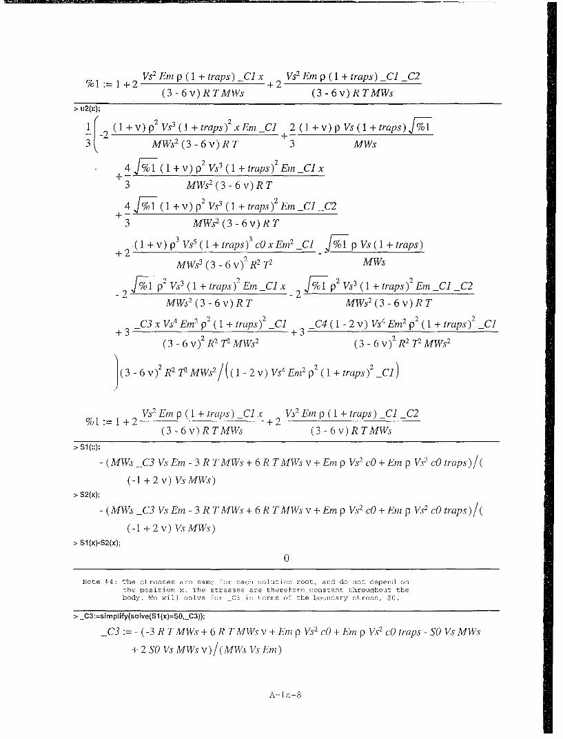
Vs2 Em p ( 1 + traps) _C]1x Vs2 Em P (1+ traps) -C1 C2%1 :-- 1 +2- +2
(3- 6v) R TMWs (3 - 6 v) R TMWs
> u2(x);
S(- 1 + v) p2 Vs3 ( 1 + traps)2 x Em -C1 2 (1 + v) p Vs (1 + traps) %1
3 MWs2 (3 - 6 v) R T 3 MWs
4 [1 ( 1 + v) p2 Vs3 (1 + traps)2 Em _Cj x
3 MWs2 (3 - 6 v) R T
4 01 ( 1 + v) p2 Vs3 (1 + traps )2 Em _C1 C2
3 MWs2 (3 - 6 v) R T
(2 +(V)P 3 Vs5(I +traps) 3 cOxEm2 _C1lF010 I p Vs(I +traps)
MWs3 (3-6 v) 2 R2 TI MWs
%2 TT%1 p2 Vs' ( 1 + traps)2 Em -C1 x %2 1 p2 Vs3 ( 1 + traps)2 Em I C2MWs2 (3 -6v)RT MWs2 (3- 6v)RT
+3 C3 X Vs4 Em2 p32 ( 1 + traps)2 _Cj C4 (1 - 2 v) VVs4 Em2 p 2 (1 + traps)2 _C1+3 - +3-
(3 - 6 v)2 R2 T2 MWs2 (3 - 6v) 2 R 2 T2 MWs2
(3-6 V) 2 R 2TVMWS2/((1 -2v) V4 EM22 ( 1 +traps )2 _C])
Vs2 Em p (1 + traps) -C1 x Vs2 Em p (1 + traps) C1 C2%1 : 1 +2 +2 -
(3 - 6v) R TMWs (3- 6v) R TMWs
"> Sl(x);
- (MWs _C3 Vs Em - 3 R TMWs + 6 R TMWs v +Em p Vs2 cO + Em p Vs2 cO traps)/(
(-1 + 2 v) Vs MWs)"> S2(x);
- (MWs _C3 Vs Em- 3 R TMWs + 6 R TMWs v +Em p Vs2 cO + Em p Vs2 cO traps)/(
(-1 + 2 v) Vs MWs)
"> S1 (x)-S2(x);
0
Note #4: The stresses are same for each solution root, and do not depend onthe position x! The stresses are therefore constant throughout thebody. We will solve for C3 in terms of the boundary stress, SO.
"> _C3:=simplify(solve(S1 (x)=SO,_C3));
_C3:= - (-3 R TMWs + 6 R TMWs v + Em p Vs 2 cO + Em p Vs2 cO traps - SO Vs MWs
+ 2 SO Vs MWs v)/(MWs Vs Em)
A-ia-8

"> S1(x);
So"> S2(x);
so"> Sl:=x->S0;
Si :=x - SO"> S2:=x->SO;
82 :=x-->SO
Note #5: Now we will introduce numerical values for the material properties.The values selected are typical for internal hydrogen as asolute in AISI 4340 steel.
"> SO:=0.0;
SO:= 0> Ds:=l e-9;
Ds:= .110-"> Vs:=2.02e-6;
Vs :=.202 10-'"> traps:=19;
traps := 19"> cO:=0.0;
cO:= 0
"> MWs:=0.00100797;
MWs :=.00100797"> Em:=200e9;
Em :=.200 1012
"> nu:=0.3;
V :=.3
"> rho:=7800;
p := 7800> T:=293;
T:= 293> R:=8.31432;
R:= 8.31432> K;
.166666666666667 1012
"> lambda;
.115384615384616 1012
"> mu;
.769230769230769 1011"> alpha;
A-ia-9

5.21047253390476"> Rh:=R/MWs;
Rh := 8248.57882675080"> Ki;
138.199274509089"> K2;
312.628352034286"> KI*K2;
43205.0114421104"> 1/(Kl*K2);
.0000231454631447068"> Al;
.4"> A2;
270.944571763048"> A3;
0>BI;
.500000000000001 1012
"> B2;
.156314176017143 1015
"> B3;
0> 03;
.00723592800000000"> SI(x);
0"> S2(x);
0
Note #6: Now let's solve for the integration constants: _Cl, _C2, and C4, using theboundary data.
"> cl (X);
.0000231454631447068 + .0000231454631447068
SIl + 86410.0228842208 _Cl x + 86410.0228842208 Cl _C2"> c2(x);
.0000231454631447068 - .0000231454631447068
I + 86410.0228842208 _Cl x + 86410.0228842208 _Cl _C2"> evalf(cl (x),5);
A-la-I0

.000023146 + .000023146 1. + 86408. _CI x + 86408. _Cl _C2"> eqnsetl :={0=cl (0),1e-6=cl (0.10));
eqnsetl := {-.1 10- =.0000231454631447068 + .0000231454631447068
J1 + 8641.00228842208 _CI + 86410.0228842208 -C1 _C2,0 =
.0000231454631447068 + .0000231454631447068 1 1 + 86410.0228842208 C1 _C2 }"> varset :={LC1 ,C2};
varsetl _ C2, -C1}"> soinsetl :=solve(eqnsetl ,varsetl);
solnseti
"> eqnset2:={O=c2(0),l e-6=c2(0.10)};
eqnset2 := { A1 10-' = .0000231454631447068
- .0000231454631447068 J 1 + 8641.00228842208 _C1 + 86410.0228842208 _C1 _C2,0=
.0000231454631447068 - .0000231454631447068 j1 + 86410.0228842208 _C1 _C2 }"> varset2:={C1 ,C2};
varset2 _ C2, Cl }"> solnset2:=solve(eqnset2,varset2);
solnset2 { CI = -.978397494278943 10-, _C2 = 0 }"> assign(solnset2);
Note #7: The solution cl(x) is not capable of satisfying the boundaryconditions, as evidenced by the lack of solution for the givenboundary conditions. The concentration function c2(x) is thecorrect solution in this case!
"> c2(x);
.0000231454631447068 - .0000231454631447068 J1 -_.845433498705078 x"> pl :=plot(le6*c2(x/l00),x=O..10,title='Concentration, c2(x) [ppm]'):"> P1;
Concentration, c2(x) [ppm]1"
0,8'
0.6
0.4
0.2
00 2 4 6 8 10x
A-la-Il
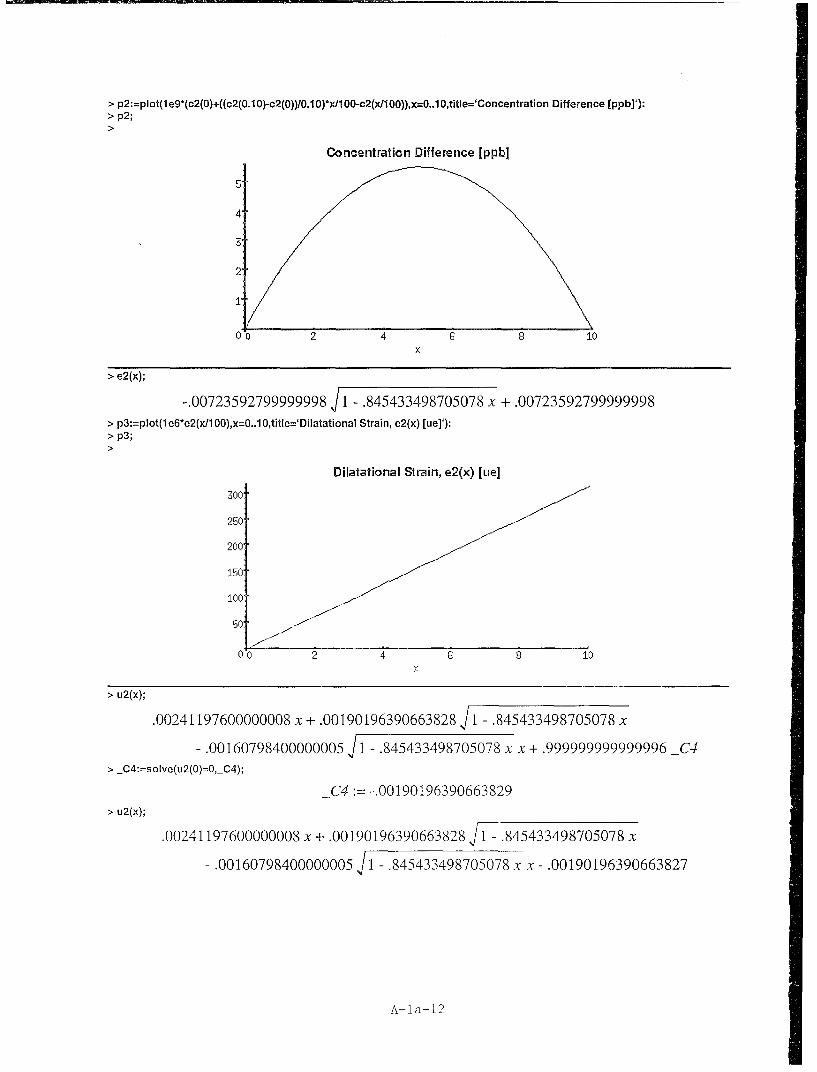
"> p2:=plot(1 e9*(c2(0)+((c2(0.1 0)-c2(0))/O.1 0)*x1 00-c2(x/I 00)),x=o..l O,title='Concentration Difference [ppb]'):"> p2 ;
Concentration Difference [ppb]
5
4
2'
0 2 4 6 8 10
x
"> e2(x);
-.00723592799999998 J 1 - .845433498705078 x + .00723592799999998"> p3:=plot(le6*e2(x/100),x=O..10,title='Dilatational Strain, e2(x) [ue]'):"> p3;
Dilatational Strain, e2(x) [ue]
300
250
200
150
100 150i
0' 2 4 6 8 iO
x
"> u2(x);
.00241197600000008 x + .00190196390663828 Ji -_.845433498705078 x
- .00160798400000005 J 1 - .845433498705078 x x + .999999999999996 _C4"> _C4:=solve(u2(0)=O,_C4);
_C4 :=-.00190196390663829"> u2(x);
.00241197600000008 x + .00190196390663828J 1 -.845433498705078 x
- .00160798400000005 J 1 - .845433498705078 x x - .00190196390663827
A-la-12

"> p4:=plot(le6*u2(x/100),x=O..10,title='Displacement, u2(x) [um]'):"> p4;
Dilatational Strain, e2(x) [ue]
300
250
200
150
100
50
00 2 4 6 8 10X
"> ex:=unapply(diff(u2(x),x),x);
1ex:= x -> .00241197600000008 - .000803991999999990 . 81J _-.845433498705078x
x+ .000679721769490914
J1 - .845433498705078 x
- .00160798400000005 j 1 - .84543 3498705078 x"> ex(x);
1.00241197600000008- .000803991999999990 . 81J _-.845433498705078x
X+ .000679721769490914/r
SI -_.845433498705078 x
- .00160798400000005 J 1 - .845433498705078 x"> p5:=plot(1 e6*ex(x/100),x=O..10,title='AxiaI Strain, ex(x) [ue]'):"> p5 ;
Axial Strain, ex(x) [ue]
100
80
GO
40
20'
00 2 4 6 8 10
A-la-13

"> evalf(u2(x),5);
.00 24 108x+.0019015 T1. -. 84542x -. 0016072 J.-.84542x x-.0019021"> evalf(c2(x),5);
.000023146 -. 000023146 J1. - .84542 x"> evalf(e2(x),5);
-.0072359 F1. - .84542 x + .0072359"> evalf(ex(x),5);
1 x.0024120-.00080399 +.00067972 .0016080 fl. - .845 4 3 x
1.-.84543 x , 1.-.84543 x
"> J2(x);
-.978397494278943 10-14
A-la-14
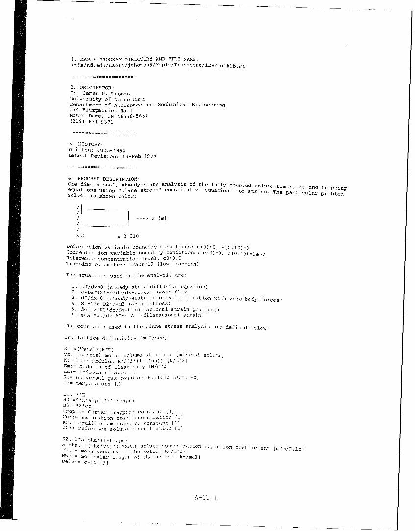
1. MAPLE PROGRAM DIRECTORY AND FILE NAME:/afs/nd.edu/user4/j thomas5/Maple/Transport/lDSSsol#lb.ms
2. ORIGINATOR:Dr. James P. ThomasUniversity of Notre DameDepartment of AerospaCe and Mechanical Engineering374 Fitzpatrick HallNotre Dame, IN 46556-5637(2i9) 631-9371
3. HISTORY:Written: June-1994Latest Revision: 13-Feb-1995
-... . = = = = -= ===
4. PROGRAM DESCRIPTION:One-dimensional, steady-state analysis of the fully coupled solute transport and trappingequations using "plane stress" constitutive equations for stress. The particular problemsolved is shown below:
--- > x [m]/ ' _ _ _ _ _ _ _ _ _
x=O x=0.010
Deformation variable boundary conditions: u(O)=O, S(O.10).OConcentration variable boundary conditions: c(O)=O, c(0.10)=le-7Reference concentration level: cO=0.0Trapping parameter: traps=19 (low trapping)
The equations used in the analysis are:
1. dJ/dx=0 (steady-state diffusion equation)2. J=Ds*(Kl*c*de/dx-dc/dx) (mass flux)3. dS/dx=G (steady-,state deformation equation with zero body forces)4. S=Bl*e-B2*c+B3 (axial stress)5. de/dx-K2*dc/dxý0 (d•iational strain gradient)6. e=Al*du/dx+A2*c.-A.i (dilatational strain)
The constants used in (ie plane stress analysis are defined below:
Ds:=lattice diffusivily Im^2/sec]
KI:=(Vs*K)/(R*T)Vs:= partial molar voihlime of solute [m^3/mol solute]K:= bulk modulus=Em/(3*(l-2*nu)) [N/m^2]Em:= Modulus of Elast icity [N/m^2]nu:= Poisson's ratio [I]R:= universal gas consant=8.31432 [J/mol-K]T:ý temperature [K)
Bl:=3*KB2:=9*K*alpha*(l+traps;)B3:=B2*cotraps:= Csr*Kr=trappilng constant [11Csr:= saturation trap concentration [i]Kr:= equilibrium trapping constant [11c00: reference so) ute( concentration [1J
K2:=3*alpha*(l+traps)alpha:= (rho*Vs)/)3WMWs)=solute concentration expansion coefficient [m/m/Delc]rho:ý mass density of the solid [kg/m^3]MWs:= molecular weight of the solute (kg/mol]Delc:= c-co [1)
A-lb-i

Al: =1-2*nuA2 : =2* (l+nu) *alpha* (l+traps)A3 :A2*cO
5. REQUIRED INPUTS:
Ds:=lattice diffusivity [m^2/sec]Vs:= partial molar volume of solute [m^3/mol solute]traps:= Csr*Kr=trapping constant [1]cO:= reference solute concentration [1]MWs:= molecular weight of the solute [kg/mol]
Em:= Modulus of Elasticity [Pa]nu:= Poisson's ratio [1]rho:= mass density of the solid [kg/m^3]
T:= temperature [K]
6. SYMBOLIC ANALYSIS:
"> Digits:=trunc(evalhf(Digits));
Digits:= 15
"> J:=Ds*(K1 *K2*c(x)-I )*diff(c(x),x);
J:= Ds (K] K2 c(x) - 1) c(x)
"> deqn:=diff(J,x)=O;
deqn::DsK]K2 c(x) +Ds(K]K2c(x)D- 1) c(x) 0
"> csoln:=dsolve(deqn,c(x),explicit);
1 +2 K2Clx+2K1K2 C1 C2_
C_ C1 +J + K K - - -csoln c(x) = - KI K2
C1K - 1 J+ 2K -K C-±K K C]C
K] K2
Note #1: There are apparently two "roots" to the solution for c(x) . Theboundary conditions will be used to select the proper one.
"> cl :=unapply(simplify(op(2,csoln[1])),x);
1x>I+ KI + 2 K1K2_C x + 2 K K2_C _C2c] : x -->
K]K2"> cl (x);
+J1 + 2 K] K2_C1 x + 2 K] K2 C] _C2
K] K2"> c2:=unapply(simplify(op(2,csoln[2])),x);
A-lb-2

c2:= X 1+J1+2K]K2 Clx+2K1K2 C] C2
K] K2"> o2(x);
-1+j1+2K1K2 Clx+2K]K2 Cl C2
K] K2
"> Ji :=unapply(simpi~fy(Ds*(K1 *I2*c1 (x)- )*diff(cl (x),x),x));
J]:=( )-4Ds CI> J1(x);
Ds C]"> J2:=unapply(simpijfy(Ds*(K1 *K2*c2(x)-l1)*diff(c2(x),x)));
J2:=( )Ds C]"> J2(x);
Ds C]
Note #2: The above results show thet both mess flux solutions ere identicelend equel to Ds*_Cl where -Cl is e constant of integration!
"> exi :=dsoIve(diff(e(x),x)-K2*diff (c1 (x),x)=O,e(x));
exl=ex)J 1+2K]K2 C'x+2K1K2 Cl C2+ C3KJ
"> el :=unapply(simplify(op(2,exl)),x);
el~ :=x1ýj+2K]K2 Clx+2K]K2 C] C2+ C3K]
K]"> el (x);
I 1+2K]K2 Clx±2K]K2 C] C2+.C3K]
K]"> ex2:=dsolve(diff(e(x),x)-K2*diff(c2(x),x)=O,e(x));
ex2= ~x =-j1±2K]K2 Clx±2K]K2 C] C2+ C3K]
"> e2:=unapply(simplify(op(2,ex2)),x);
e2:x-->J +2K]K2 C'x±2K]K2 C] C2- C3K]-K]
"> e2(x);
J1±2K]K2 Clx+2K]K2 C] C> -C3K]
K]
A-lb -3

"> uxi :=dsolve(A1 ~diff(u(x),x)+A2*c1 (x)-A3-el (x)=O,u(x));
uxl=u(x) = (-3 A2 x KJK2 _C1- A2 %1 I- 2 %o,1 A2 KJK2 Cl x3
-2%A2 K1K2 _C] _C2 +3A3XK12K22 _CJ±+0/ %1K2 +2 %O1 K22 K1 Cl X
+210%11K2 2 K1 Cl _C2 +3 _C3 xK12 K2 2 _CJ +3 _C4 A1K12 K2 2 _Cw)/(Al K12
K22 _Cl)
% 1:1 + 2 KK2 _Cl x+ 2 KlK2 -Cl _C2"> ul :=unapply(simplify(op(2,uxl)),x);
ul := x--> (3 A2 x KK2 -Cl +A2 jI+ 2 K1K2 _Cl x+ 2 K1K2 -Cl _C23
+ 2J11 + 2 KK2 _Cl x+ 2 K1K2 -Cl _C2 A2 KJK2 -Cl x
+ 2 J1 +2 K1K2 _Cl x+ 2 K1K2 _C] _C2 A2 K]K2 -Cl _C2 -3 A3 x K]2 K22 C]
IJ+±2 K1K2 _Cl x+ 2 K1K2 _C] _C2 K2
-2jFl+ 2 KK2 _Cl x+ 2 K1K2 -Cl _C2 K22 K -Cl x
-2 11±+2 K1K2 _Cl x+ 2 K1K2 _C] _C2 K2 2 K -Cl _C2 -3 -C3 xK12 K22 -Cl
-3 _C4 A] KJ2 K22C1)/(AJ K]2 K22KCl)"> ul (X);
-(3 A2 x KK2 _CJ +A2 %1± +2 % IA2 K]K2 _Cl x +2 %1 A2 KJK2 _C] _C23
-3A3 xK12 K2 2 _C]- % - %1KK _Cx- 2 %1 IK22 K] Cl _C2
-3 _C3 xK12 K22 _C] -3 _C4 A] K]2 K22 _Ci )/(A] K12K22 _C])
%1:= 1± 2 KK2 _Cl x±+2 K1K2 -Cl _C2"> ux2:=dsolve(A1 *diff(u(x),x)+A2*c2(x)-A3-e2Cx)=O,u(x));
ux2:= u(x) (-3 A2 xK] K2 _Cl +A2 %1± +2 [%/1IA2 KlK2 -Cl x3
+2%A2 KJK2 _C] _C2±+3 A3xK12 K22 _C]-_ 0%11K2-2 F%1IK22K] Cl x
-2,10%1K22 K] Cl _C2±+3 _C3 XK]2 K22 _C] +3 _C4 A] K12 K22 _C] )/(A] K]2
K22 _Cl)
% I:= I+ 2 KlK2 _ Clx+ 2 K]K2 _C] _C2"> u2:=unapply(simplify(op(2,ux2)),x);
u2:= x >(-3 A2 x KK2 -C]+A2 JI±+2 K]K2 _Cl x +2 K]K2 _C] _C23
A-lb -4
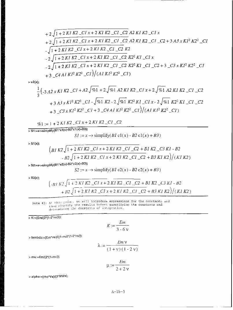
+2 1±2K1K2 Clx+2K1K2 Cl _C2A2KJK2 Clx
+2 fj1±2K1K2-Cx212Cl _C2A2KJK2 Cl _C2±3A3xK12K22 Cl
ýj + 2 KlK2 Cl x+ 2 K1K2 -Cl _C2K2
2 l+ 2 K1 K2 -Cllxx +F2 K1K2 -Cl _C2 K22 K1 Cl X
2.](1+ 2 K1K2 -CIxx++'2K1 K2 _C] _C2 K22 K1 Cl _C2 +3 _C3 XK12 K22 Cl
+ 3 _C4 Al K]2 K22 iii )/(AJ K]2 K22 _Cl)"> u2(x);
!(-3 A2 xKIK2-CI]+A2 %01o+ 2 %1olA2 KJK2 _Cl x+ 2 %1olA2 K]K2 -Cl _C23
3A3 xK]2 K22 _Cl_ /01K2 -2 %1o1K2 2 K _l- 2 %K 2 K lC
*±3 _C3 xK12 K22 _C1 +3 _C4 AlJKl2K22K-C])/(Al K]2K22KCl)
%I:I + 2 K1K2 _C] x+ 2 K]K2 -CI _C2
"> Si :=X->simplIfy(BP3l o(x).82*c1 (x)+63);
Si : x -> simplify(B] el(x) - B2 cl(x) + B3)
">51(X);
(13IK2J1+2K1K2-Clx±2K1K2 Cl _C2+B]K2 _C3K]-B2
- B2 fl+ 2 K]K2 _C x + 2 K]K2 _C] _C2±+B3 K]K2)/(K] K2)
"> S2 :=x->simlipIfy(B3lo2(x)-B2*c2 (x)+B);
S2 :=x --- simplify(B] e2(x) - B2 c2(x) + B3)
"> S2(x);
(I-lK2Ji±2K1K2-Clx+2K1K2 ClC2±B]K2 _C3Kl-B2
+ B2 j1±ý2 K1K2 _-Cl x+ 2K1 K2 -Cl _C2±+B3 KlK2)/(Kl K2)
Note #3: Al lhii'; 1"iflfl we will introduce expressions for the constants and
,ilplf the results before quantifying the constants and
~ ~iiiniigthe constants of integration.
Em
3 -6 v
> Iambda:=(EmflUi)/((l +nu)*(l-2*nu))
Em v
(1 +v) (I - 2v)
> mu:=Em/(2*(1+nU));
Em
2±+2 v> alpha:=Crho*Vs)/(3MWS);
A-Ib-5

I p Vs
3 MWs"> K1 :=(Vs*K)/(R*T);
Vs EmK]:=
(3 -6v)R T"> K2:=3*alpha*(l +traps);
K2 p Vs ( 1 + traps)
MWs"> KI*K2;
VS2 Em p (1 + traps)
(3 - 6 v) R TMWs"> A1 :=(1 -2*n u); •
A]:= 1 -2v"> A2:=2*(l+nu)*alpha*(l+traps);
2.(1 +v) p Vs(1 + traps)A2 :3 MWs
"> A3:=A2*cO;
2 (1 +v) p Vs (1 + traps) cO
3 MWs"> B3 :=3*K;
EmB]:= 3 -
3 -6v"> B2:=9*K*alpha*(1 +traps);
B2 := 3 Em p Vs (1 + traps)
(3 - 6 v) MWs"> B3:=B2*cO;
Em p Vs ( 1 + traps) cOB3 :=3(3 - 6 v) MWs
A-lb-6

> cl (x);
1+ 1+2 Vs' Emp(1+traps)-lx +Vs 2 Em p(+traps-Cl (3-6v)RT(3 - 6 v) R TMWs (3 - 6 v) R TMWs
MWs/(Vs2 Em p (1 + traps))
> c2(x);
V+s 1 2 EM p(1+trapsC V+2 Em p(1+traps) C2v)RT(3 - 6 v) R TMWs (3 - 6 v) R TMWs
MWs/(Vs2 Em p (1 + traps))
> el (x);
I VS2 Em p(1 + traps) Cl x Vs2 Em p ( 1 + traps) Cl C2 C3 Vs Em~ 11+2 -_2-(3 - 6 v) R TMWs (3 - 6 v) R TMWs (3 - 6 v) R T
(3 - 6 v) R T/(Vs Em)"> e2(x);
(J Vs2 Em p (1 + traps) Vs2 Emp(1 traps)C C2 C3 Vs Em-1+2 ±+2
(3 - 6 v) R TMWs (3 - 6 v) R TMWs (3 - 6 v) R T
(3 - 6 v) R T/(Vs Em)
"> ul(x);
i + (1 +v)ps3 (1 +traps)2 xEm _C] 2(1 +v)p Vs(1 +traps) %1-- 23 MW s2 (3 -6 v) R T 3 MWs
4 (1 + v) p 2 Vs3 (1traps) 2 EmC1_
3MWs 2 (3 -6 v) R T
4 %1 (1±V)p2 Vs3(1 +traps)2 EIJI _C] C2
-2 (1 +v ) p 3 Vs (1 l +traps )3 cO xErn2 _Cl _%,1 p Vs (1 +traps )MWs (3 -6 v)2 R2T2 MWs
+ V1 p3 Vs3 (I + traps) Em C x % I p Vs3 ( + traps) EmCJ C2
-2 - 2MWs2 (3 - 6 v) R T MWs2 (3 - 6 v) R T
C3 x Vs4 Em2p 2 ( 1 + traps )2 _Cl C4 (1 - 2 v) Vs4 Em2 p2 (1 + traps)2 C](36v)2 R2 T2 MWs2 (3-6 v) 2 R2 2 MWs2
(3-6V) 2 R2 VMWs2 /((1 - 2 v) Vs4 Em2 p2 ( 1 + traps)2 C])
Vs2 Em p (1 + traps) _C1 x Vs2 Em p(1 + traps) C1 C2%1 :1 + 2 +2
(3 - 6 v) R TMWs (3 - 6 v) R TMWs
A-lb-7

> u2(x);
+(- (l 2v)p2 Vs3(+1traps)2 xEm-C1 2 (1+v)pVs(1+traps) %1
MWs2 (3 - 6 v) R T 3 MWs
4 %1I ( 1 + v) p2 Vs3 (1 + traps)2 Em _C C X
3 MWs2 (3 - 6 v) R T
+420M (1 +V) P2 Vs3 (1 + traps )2 EM _Cl sC2
3 MWs2 (3 - 6v) R T+2 (+V) p3 VS,(1I + traps)3cO x Em2_Cj C10 p Vs(1 +traps)
-2 -2 FMWs3 ( 3 -6 V )2 R 2 T2 MWs
-2 1p2 Vs3 ( 1 + traps )2 Em -C1 x_ 2 /0 p 2 Vs3 (I1 + traps )2 Em _C1 _C2
MWs2 (3 - 6 v) R T MWs2 (3 - 6 v) R T
C3 X Vs4 Em2 p2 (1 + traps)2 _C1 C4 (1 - 2 v) Vs4 Em2 p 2 (1 + traps)2 _C]+3 - +3
(3 - 6 v)2 R2 72 TMWs2 (3-6 v) 2 R2 T2 MWs2
)(3-6 V)2 R 2 TiMWS2 /((I -2V) VS4Em2 p2 (1 +traps)2 _Cj)
Vs2 Em p (1 + traps) Cl x Vs2 Em p (1 + traps) _C C2%1:=1+2 +2 _
(3 - 6 v) R TMWs (3 - 6 v) R TMWs
"> S1(x);
- (MWs _C3 Vs Em - 3 R TMWs + 6 R TMWs v +Em p Vs 2 cO + Em p Vs2 cO traps)/(
(-1 +2v) VsMVLs)"> S2(x);
- (MWs _C3 Vs Em - 3 R TMWs + 6 R TMWs v +Em p Vs2 cO +Em p Vs2 cO traps)/(
(-1 + 2 v) Vs MWs)
"> SI(x)-S2(x);
0
Note #4: The stresses are same for each solution root, and do not depend onthe position x! The stresses are therefore constant throughout thebody. We will solve for C3 in terms of the boundary stress, SO.
"> C3:=simplify(soIve(S1 (x)=SO,_C3));
_C3:= - (-3 R T MWs + 6 R T MWs v + Em p Vs 2 cO + Em p Vs2 cO traps - SO Vs MWs
+ 2 SO Vs MWs v)/(Em MWs Vs)"> S1 (x);
SO"> S2(x);
A-lb-8

So"> Si :=x->SO;
Si := x SO"> S2:=x->SO;
S2 :=x- SO
Note #5: Now we will introduce numerical values for the material properties.The values selected are typical for internal hydrogen as asolute in AISI 4340 steel.
"> So:=0.0;
SO:= 0"> Ds:=le-9;
Ds:= .1 10-8
> Vs:=2.02e-6;
Vs :=.202 10-5"> traps:=19;
traps := 19"> cO:=0.O;
cO:= 0"> MWs:=0.00100797;
MWs :=.00100797
> Em:=200e9;
Em :=.200 1012
"> nu:=0.3;
V :=.3
"> rho:=7800;
p := 7800
"> T:=293;
T:= 293
"> R:=8.31432;
R:= 8.31432
> K;
.166666666666667 1012
"> lambda;
.115384615384616 1012
"> mu;
.769230769230769 1011
"> alpha;
5.21047253390476
"> Rh:=R/MWs;
A-lb-9

Rh:= 8248.57882675080"> K1;
138.199274509089"> K2;
312.628352034286"> KI*K2;
43205.0114421104"> 1/(Kl*K2);
.0000231454631447068"> Al;
.4
"> A2;
270.944571763048"> A3;
0"> B1;
.500000000000001 1012
"> B2;
.156314176017143 1015"> B3;
0> 03;
.00723592800000000"> Sl(x);
0"> S2(x);
0
Note #6: Now let's solve for the integration constants: _C, _C2, and _C4, using theboundary data.
"> ci(X);
.0000231454631447068 + .0000231454631447068
j1 + 86410.0228842208 _C] x + 86410.0228842208 Cl _C2"> c2(x);
.0000231454631447068 - .0000231454631447068
J + 86410.0228842208 _C] x + 86410.0228842208 _CI _C2"> evalf(cl(x),5);
.000023146 + .000023146 j 1. + 86408. _C] x + 86408. CI _C2
"> eqnsetl :={O=cl (0),1 e-7=cl (0.1 0)};
A-lb-10

eqnset] := { 0 =
.0000231454631447068 + .0000231454631447068 J 1 + 86410.0228842208 _C1 _C2,
.1 10-6 = .0000231454631447068 + .0000231454631447068
I1 + 8641.00228842208 _C1 + 86410.0228842208 _C1 _C2 }"> varsetl:={_C1,_C2};
varset] -_Cl, -C2}"> soinsetl :=solve(eqnsetl,varsetl);
solnset]
"> eqnset2:={O=c2(O),1 e-7=c2(0.1 O)};
eqnset2 :={ 0 =
.0000231454631447068 - .0000231454631447068 J1 + 86410.0228842208 _Cl _C2,
.1 10-6 = .0000231454631447068
- .0000231454631447068 J 1 + 8641.00228842208 _Cl + 86410.0228842208 _Cl C2
}"> varset2:={_C1,-C2};
varset2 -C], _C2"> solnset2:=solve(eqnset2,varset2);
solnset2 := { -C = -.997839749427893 10-6, _C2 = 0"> assign(solnset2);
Note #7: The solution cl(x) is not capable of satisfying the boundaryconditions, as evidenced by the lack of solution for the givenboundary conditions. The concentration function c2 (x) is thecorrect solution in this case!
"> c2(x);
.0000231454631447068 - .0000231454631447068 J1 - .0862233555828494 x"> pl :=plot(le6*c2(xl OO),x=O..1O,title='Concentration, c2(x) [ppm]'):
"> P;
Concentration, c2(x) [ppm]0.1'
0,08'
0,06'
0.047
0.027
2 4 8 8 10
A-lb-li

"> p2:=plot(1 e9*(c2(O)+((c2(O.1 O)-c2(O))IO.1 O)*x/l O-c2(x/l OO)),x=O..1 O,title='Concentration Difference [ppb]'):"> p2;
Concentration Difference [ppb]
0.04
0.03
0.00
"> e2(x);
-.00723592799999998 1i -_.0862233555828494 x + .00723592799999998"> p3:=plot(1e6*e2(xI100),x=O..1O,title='Dilatational Strain, e2(x) [ue]'):"> p3;
Dilatational Strain, e2(x) [ue]
30
25
20
15
100
"> u2(x);
.00241197600000003 x +.0186490538338527I Ji-.0862233555828494 x
- .001607984000000021 -_.0862233555828494 xx +.999999999999992_C4"> C4:=solve(u2(O)=O,-C4);
-C4: -.0186490538338528"> u2(x);
.00241197600000003 x +.018649053833852711 -.0862233555828494)x
- .00160798400000002 Ji1 -_.0862233555828494 x x - .0186490538338526
A-Ib--12

"> p4:=plot(1e6*u2(x/100),x=O..10,title='Displacement, u2(x) [urn]'):"> p 4 ;
Displacement, u2(x) [um]
0.5
0.4
0.3
0.2
0.1
00 2 4 6 8 10X
"> ex:=unapply(diff(u2(x),x),x);
1ex := x -4 .00241197600000003 - .000803991999999991 .0J1 -. 0862233555828494x
X+ .0000693228881017671
Ji - .0862233555828494 x
-. 00160798400000002J 1 -_.0862233555828494x"> ex(x);
1.00241197600000003- .000803991999999991 .0S1 l-.0862233555828494x
x+.0000693228881017671 lJ 1_-.0862233555828494x
- .00160798400000002J 1 - .0862233555828494x"> p5:=plot(1 e6*ex(x/100),x=O..10,title='Axial Strain, ex(x) [ue]'):"> p5;
Axial Strain, ex(x) [ue]
10
8!
4
2
00 2 4 6 8 10x
A-lb-13

"> evalf(u2(x),5);
.0024107x+.018644 1. -. 086222x-.0016072 1.-.086222xx-.018 6 5 0"> evalf(c2(x),5);
.000023146-.000023146 1.- .086222x"> evalf(e2(x),5);
-.0072359 F1. - .086222 x + .0072359"> evalf(ex(x),5);
1 x.0024120 - .00080399 + .000069323
ý1. -. 086223x 1.-.086223x
- .0016080 1 1. - .086223x
"> J2(x);
-.997839749427893 10-15
A-lb-14

1. MAPLE PROGRAM DIRECTORY AND FILE NAME:/afs/nd.edu/user4/jthomas5/Maple/Transport/lDSSsol#lc.ms
2. ORIGINATOR:Dr. James P. ThomasUniversity of Notre DameDepartment of Aerospace and Mechanical Engineering374 Fitzpatrick HallNotre Dame, IN 46556-5637(219) 631-9371
3. HISTORY:Written: 21-Jan-1995Latest Revision: 13-Feb-1995
4. PROGRAM DESCRIPTION:One-dimensional, steady-state analysis of the fully coupled solute transport and trappingequations using "plane stress" constitutive equations for stress. The particular problemsolved is shown below:
'I I/1 I --- > x [m]'I I
x=O x=0.010
Deformation variable boundary conditions: u(O)=O, S(0.10)=OConcentration variable boundary conditions: c(0)=O, c(0.10)=le-7Reference concentration level: cO=0.0Trapping parameter: traps=499 (high trapping)
The equations used in the analysis are:
1. dJ/dx=O (steady-state diffusion equation)2. J=Ds*(Kl*c*de/dx-dc/dx) (mass flux)3. dS/dx=O (steady-state deformation equation with zero body forces)4. S=Bl*e-B2*c+B3 (axial stress)5. de/dx-K2*dc/dx=O (dilational strain gradient)6. e=Al*du/dx+A2*c-A3 (dilatational strain)
The constants used in the plane stress analysis are defined below:
Ds:=lattice diffusivity [m^2/sec]
Kl:=(Vs*K)/(R*T)Vs:= partial molar volume of solute [m^3/mol solute]K:- bulk modulus=Em/(3*(l-2*nu)) [N/m^2]Em:= Modulus of Elasticity [N/m^2]nu:= Poisson's ratio [1]R:= universal gas constant=8.31432 [J/mol-K]T:= temperature [K]
BM:=3*KB2:=9*K*alpha*(l+traps)B3:=B2*cotraps:= Csr*Kr=trapping constant [1)Csr:= saturation trap concentration [1]Kr:= equilibrium trapping constant [1]cO:- reference solute concentration [1]
K2 :3*alpha*(l+traps)alpha:= (rho*Vs) / (3* MWs)=solute concentration expansion coefficient [m/m/Delc]rho:- mass density of the solid [kg/m^3]MWs:= molecular weight of the solute [kg/mol]Delc:= c-cO [1]
A-IC-I
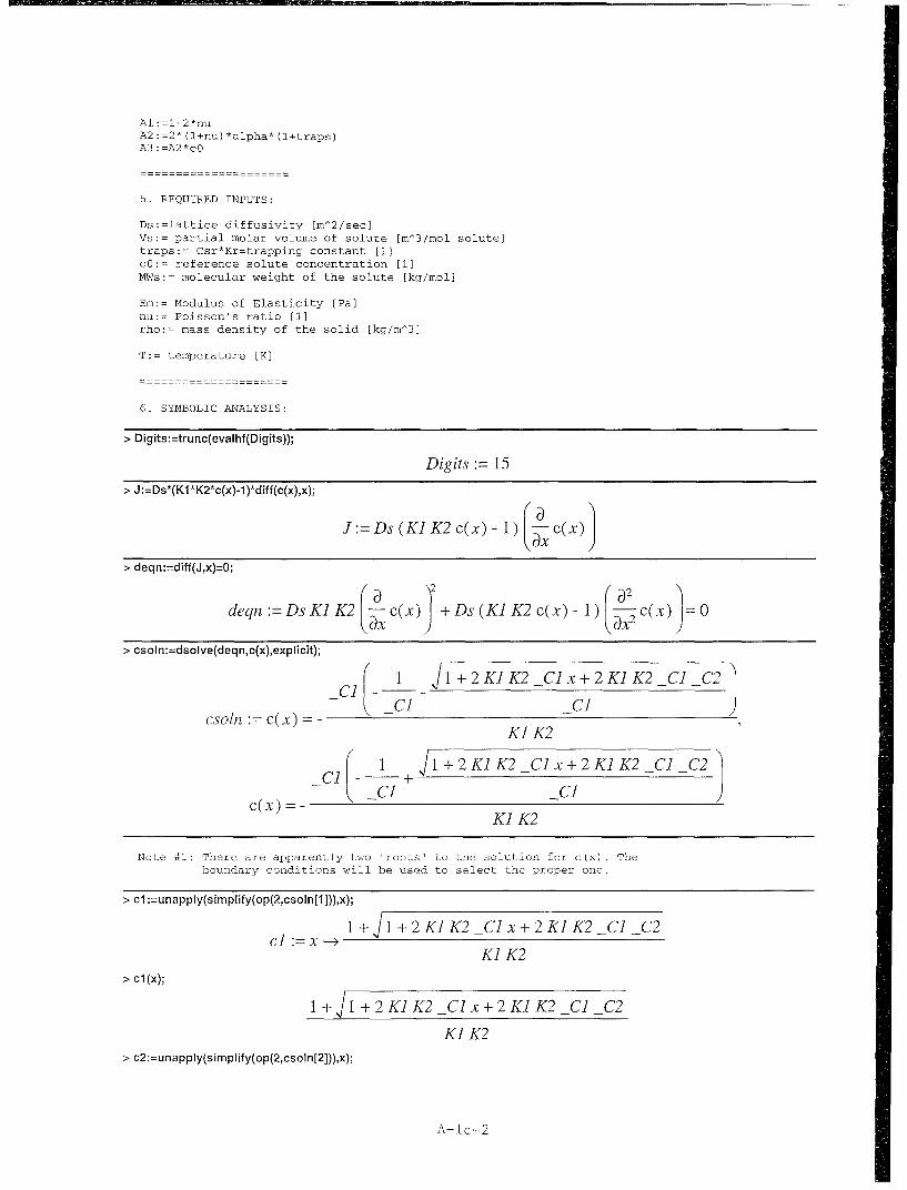
Al: =l-2*nuA2:=2*(l+nu)*alpha* (l+traps)A3 : =A2*cO
5. REQUIRED INPUTS:
Ds:=lattice diffusivity [m^2/sec]Vs:= partial molar volume of solute [m^3/mol solute]traps:= Csr*Kr=trapping constant [1]cO:= reference solute concentration [1]MWs:= molecular weight of the solute [kg/mol]
Em:= Modulus of Elasticity [Pa)nu:= Poisson's ratio [1]rho:= mass density of the solid [kg/m^3]
T:= temperature [K]
6. SYMBOLIC ANALYSIS:
"> Digits:=trunc(evalhf(Digits));
Digits:= 15
"> J:=Ds*(Kl*K2*c(x)-l)*diff(c(x),x);
J:= Ds (K] K2 c(x) -1) c(x)
"> deqn:=diff(J,x)=O;
deqn :=DsK] K2 -c(x) +Ds(K]K2c(x)-l) - c(x) 1
"> csoln:=dsolve(deqn,c(x),explicit);
C C1 - C]csoln := C(x) cK KC
C JI +2K]K2 Clx+2K]K2 C1 C2
C()=- _ C1 K K2_01
K] K2
Note #1: There are apparently two "roots" to the solution for c(x) . Theboundary conditions will be used to select the proper one.
"> cl :=unapply(simplify(op(2,csoln[1])),x);
1x + I + 2 K] K2 _C1 x + 2 K] K2 _C] _C2Ci : x -->
K] K2"> cl (x);
1 +J1 +2KI K2 C1x+2K] K2 C] C2
K] K2"> c2:=unapply(simplify(op(2,csoln[2])),x);
A-Ic-2

c2 = x -1±J1±2K]K2 Clx+2K]K2 C] C2
K] K2"> c2(x);
-1 +J11 + 2 K K2 -CIx + 2 K K2 -CI C2
K] K2
"> Ji :=unapply(simplify(Ds*(K1 *K2*c1 (x)-1 )*diff(c1 (x),x),x));
> A (X);
Ds CI"> J2:=unapply(simplify(Ds*(K1 *K2*c2(x)..1)*dlff(c2(x),x)));
J2:= )-Ds -Cl"> J2(x);
Ds CI
Note #~2: The above results show that both mass flux solutions are identicaland equal to Ds*-Cl where -Cl is a constant of integration!
"> exi :=dsoIve(diff(e(x),x)-K2*diff (d1(x),x)=O,e(x));
ex]:=e() J + 2 K]K2 -C] x+ 2 K]K2 -C] C2 + -C3 K
"> el :=unapplIy(s imp] ify(op(2,exI)),x);
eli:= X >1±+2 K]K2 -C] x+ 2 K]K2 -C] C2±+ C3 K]K]
"> el (x);
I + 2 K K2 -C] x+ 2 K1K2 -C] -C2+ -C3 KK]
"> ex2:=dsolve(diff~e(x),x)-K2*diff(c2(x),x)=O,e~x));
JI 1+ 2 K K2 -C x + 2K]K2 -C] C2 - ýC3 Kex2: e(x) = - .K]
"> e2:=unapply(simplify(op(2,ex2)),x);
e2 :=x-)>-u1±2K]K2 Clx+2K]K2 C] C2- C3KIK]
"> e2(x);
-J 12K]K2 Clx±2K]K2 C] C2- C3K]
K]
A- Ic-3
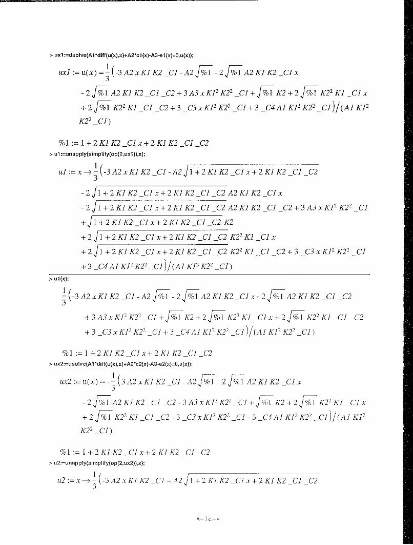
"> uxi :=dsolve(A1 *diff (u~x),x)+A2*cl (x)-A3-el (x)=O,u(x));
uxl :=u(x) = 3(-.3A2 x KJK2 _C] -A2 % I- 2 %1l IA2 K]K2 -Cl x
-2 %1ColA2 K]K2 _C] _C2±+3 A3 XK12 K22 _C] + %10,K2 +210/0K2 2 K Cl x
+ 2 %1 00K22 K] _C] _C2 +3 _ C3 XK12K22 _C] +3 _C4 A] K]2 K2 2 _C])/(AiK12
K22 _C])
%1I:= 1 + 2 KK2 _Cl x±+2 K]K2 _C] _C2"> ul :=unapply(simplify(op(2,uxl)),x);
u] := x --->-3 A2 x K]K2 -C]- A2 jI+ 2 K]K2 _Cl x+ 2 K]K2 _C] _C23
- 2J1 +2 K]K2 _Cl x±+2 K]K2 _C] _C2 A2 K]K2 -Cl x
- 2J1±+2 K]K2 _Cl x+ 2 K]K2 -C] _C2A2 K]K2 -Cl _C2±+3 A3 XK]2 K22 _ C]
*±j1±+2 K]K2 _Cl x +2 K]K2 _C] _C2 K2
* 2 JI±+2 K]K2 _Cl x±+2 K1K2 -Cl _C2 K22 K -Cl x
*±2J11±+2 K1K2 _Cl x±+2 K1K2 _C] _C2 K22 K1 Cl _C2 +3 -C3 XK12K22 _ C]
*±3 C4 A]JK12 K22 -_C]) /(A] K]2K22 _C])"> ul(x);
'(-3A2 x KIK2 _C] -A2 FI- 2 %1 A2 K]K2 _Cl x -2 %1 A2 K]K2 _C] _C23
*±3A3 x K1 2K22 _C]± +%1 IK2±+2 %1 ,K2 2 K _Cl x±+2 %17,lK2 2K] _C] _C2
*±3 _C3 x K]2K22 _C]±+3 _C4 A] K]2 K22 _C])/(A] K12 K22 C])
%1I:= I1+2 K]K2 _Cl x±+2 K]K2 _C] _C2"> ux2:=dsolve(A1 *diff(u(x),x)+A2*c2(x)-A3-e2(x)=o,u(x));
tx2 := u(x>-(3 A2 x K]K2 _C] -A2 % I- 2 %1l IA2 K]K2 -Cl x3
-2 %1/-lA2 K]K2 _ C] _C2-3 A3 x K12K22 _C]± +%1 K2±+2 J% 1K2 2 K] Cl x
+ 2 % /11 K22 K] _C] _C2 -3 _C3 xK]2 K22 _C] -3 _C4 A] K]2 K22 _C] )/(A] K]2
K22 _C])
%1I:= I +2 K]K2 _Cl x±+2 K]K2 _C] _C2"> u2:=unapply(simplify(op(2,ux2)),x);
u2:= x- (-3 A2 x KK2 -C]±+A2 J±+2 K]K2 _C] x±+2 K]K2 _C] _C23
A-le-4

+2J1 +2K1 K2 _Clx+2K1K2 C _C2 A2K K2 _Cix
+2J1 +2KJ K2 _Clx+2KK2 Cl _C2 A2K K2 C _C2+3A3xK12 K2 2 _C1
-J1 +2K1K2 Cx+2K1K2 Cl _C2 K2
-2J1 +2K1K2 _Cx+2KK2 Cl _C2 K22 K1 _Ci x
- 2 j 1 + 2 K1 K2 _C1 x + 2 K1 K2 _C1 _C2 K22 K1 _CI _C2 + 3 _C3 x K12 K2 2 _C1
+ 3 _C4 A] K12 K22 _C1)/(Al K12 K22_CJ)"> u2(x);
±(-3 A2 xK1K2 _CIJ+A2 J5.1+ 2 %10o1A2 KK2 _Ci x±+2 %1/A2 KJK2 -Cl _C23
+3A3XK12K22 Cl- 12- %12K _Cix-210%1lK22KJ Ci _C2
+ 3 _C3 x K12 K22 _CI + 3 _C4 Al K12 K22 _C1 )/(A] K12 K22 _CI)
%1:= 1 + 2 KJ K2 _Ci x + 2 KJ K2 _C1 _C2
"> Si :=x->simplify(B1*el(x)-B2*cl(x)+B3);
Si :x - simplify(B! el(x) - B2 cl(x) + B3)
"> S1 (x);
(B1 K2 J1 + 2 K1 K2 _Cl x + 2 K1 K2 _C1 _C2 + BJ K2 _C3 KJ - B2
- B2 j 1 + 2 K1 K2 _Cl x + 2 K1 K2 _C] _C2 + B3 KJ K2)/(KJ K2)"> S2:=x->simplify(B l*e2(x)-B2*c2(x)+B3);
S2 := x -- simplify(B! e2(x) - B2 c2(x) + B3)"> S2(x);
- (BI K2 J 1 + 2 K1 K2 _CI x + 2 K] K2 _CI _C2 - B] K2 _C3 KJ + B2
- B2 J 1 + 2 K1 K2 _C] x + 2 K1 K2 _C] _C2- B3 K K2)/(K] K2)
Note #3: At this point, we will introduce expressions for the constants andthen simplify the results before quantifying the constants anddetermining the constants of integration.
"> K:=(Em/(3*(1-2*n u)));
EmK:= 3-6v
"> Iambda:=(Em*nu)/((l+nu)*(1-2*nu));
Em v
(1+v)(1 -2v)"> mu:=Em/(2*(l+nu));
Em2+2v
"> alpha:=(rho*Vs)/(3*MWs);
A-Ic-5

I p Vs
3 MWs"> K1 :=(Vs*K)/(R*T);
Vs EmK1.-
(3 -6v)RT"> K2:=3*alpha*(1 +traps);
p Vs ( 1 + traps)K2 :MWs
"> KI*K2;
Vs2 Em p (1 + traps)
(3 - 6 v) R TMWs"> A1:=(1-2*nu);
Al:= 1 -2 v"> A2:=2*(l +nu)*alpha*(l +traps);
2 (1 +v)p Vs(1 +traps)A2:=3 MWs
"> A3:=A2*cO;
2 (1 +v) p Vs (1 +traps) cOA3 =-3 MWs
"> B1 :=3*K;
Em3-6v
"> B2:=9*K*alpha*(1 +traps);
Em p Vs (1 + traps)B2 :=3(3 - 6 v) MWs
"> B3:=B2*cO;
Em p Vs (1 + traps) cOB3:=3(3 - 6 v) MWs
A-ic-6

"> cl (X);
(1+ 1+2 Vs2 Emp(1+traps) Clx Vs + 2 Emp(I+traps) Cl C2 (3 6v)RTJ (3 -6v) RTMWs (3 - 6v) RTMWsMWs/(Vs2 Em p (1 + traps))
"> c2(x);S / Vs2 Em p(1+ traps) -Cl x Vs2 Em p( 1+ traps) -C1 C21
-f1+j1+2 Vs +2 -- (-vR1 (3 - 6 v) R TMWs (3 - 6 v) R TMWs
MWs/(Vs2 Em p (1 + traps))
"> el(x);
r Vs2 Em l(+traps) Clx Vs2 Emp(1+traps) _C1 C2 C3VsEmJ1+2 (3-6v)RTMWs (3-6v)RTMWs (3-6v)RTT
(3 - 6 v) R T/(Vs Em)"> e2(x);
Vs2 Emp(1 +traps)xmC 2 sEmp(1 + traps)( CC2 C3 Vs Em1+ -+2 _ _ _ _ _ _ _ _ _ _
(3 - 6 v) R TMWs (3 -6v)RTMWs (3-6v)RT(3 -6 v)R T/(Vs Em)
"> ul(x);
1 2(1 +V) p 2 Vs3(1 +traps)2 xEm _Cl 2 (1 +v) pVs (I1+traps) %oo1.3MWs 2 (3 -6 v) RT 3 MWs
4 1,I ( 1 + v) p2 Vs3 ( 1 + traps)2 Em _Cl x3 MWs2 (3 - 6 v) R T
4 %1I ( 1 + v) p 2 Vs3 ( 1 + traps)2 Etmi Cl _C2
3 MWs2 (3 - 6 v) R T
+(2 +v)p 3 Vs5( +traps) 3 cOxEm_ Cl +%l p Vs( +traps)+ 2 +
MWS3 (3-6 V)2R 2 7 MWs2 )2 2 s+2,Fo p Vs3 (1+ traps) Em Cl x + %2 1 p 2 Vs 3 (1+ traps) 2Em C1 C2+2 +2--MWs2 (3 - 6v)R T MWs2 (3 - 6v)R T
C3 x Vs4 Em2 (p1 + traps )2 _1 C4 (1 - 2 v) Vs4 Em2 p2 ( 1 + traps)2 _C
(3 - 6 v) 2 R2 V MWs2 (3 - 6 v)2 R2 T2 MWs2
) (3-6v)2 R2 72MWS2/((I -2v) Vs4 Em2P2 (1 + traps)2 _Cl)
A-ic-7

VS2 Em p (1 + traps) C1 x Vs2 Em p ( 1 + traps) -1 C2
% 1:= 1 + 2(3-6v)RTMWs (3-6v)RTMWs
> u2(x);
1 -2 +V ( 1 + traps)2 x Em CI 2 (1 + v) p Vs ( 1 + traps) 7% 1-2
3 MWs2 (3 - 6 v) R T 3 MWs
4 j% ( 1 + v) P2 Vs3 (I + traps)2 Em C1x
3 MWs2 (3 - 6v) R T
4 O% ( 1 + v) p2 Vs3 (1 + traps)2 Em Cl C2
3 MWs2 (3 -6v)RT
+2 (1+v)p3 Vs 5(1+traps)3 cOxEm2 _Cl] % pVs(1+traps)M~336) 2 R2T MWsMWsI (3 - 6 V2R2 T2 w
%I 2• -2 Vs3 (1 + traps)2 EmraC1 x 2%1 92 Vs3 (I + traps)2 Em Cl C2
MWs2 (3 - 6 v) R T MWs2 (3 - 6 v) R T
3 C3 x Vs4 Em2 p2 ( 1 + traps)2 C1 C4 (1 - 2 v) Vs4 Em2 p2 (1 + traps)2 C1
(3-6 V) 2 R2 2MWs2 (3-6 v)2 R 2 T2 MWs2
(3-6 v) 2R2 TIMWS2/(( 1 -2V) VS4 EM2P2 ( 1+ traps )2 _Cl)
Vs2 Em p (1 + traps) -C1 x Vs2 Em p (1 + traps) -C1 C2%1 := 1 +2 +2
(3 - 6 v) R TMWs (3 - 6 v) R TMWs
"> S1(x);
- (MWs _C3 Vs Em- 3 R TMWs + 6 R TMWs v + Em p Vs2 cO +Em p Vs2 cO traps)/(
(-1 +2v) VsMWs)"> S2(x);
- (MWs _C3 Vs Em - 3 R TMWs + 6 R TMWs v + Em p Vs2 cO +Em p Vs2cO traps)/(
(-1 + 2 v) Vs MWs)
"> Sl(x)-S2(x);
0
Note #4: The stresses are same for each solution root, and do not depend onthe position x! The stresses are therefore constant throughout thebody. We will solve for _C3 in terms of the boundary stress, SO.
> C3:=simplify(solve(Sl(x)=SO,_C3));
_C3:= - (-3 R TMWs + 6 R TMWs v + Em p Vs 2 cO + Em p Vs2 cO traps - SO Vs MWs
+ 2 SO Vs MWs v)/(Em Vs MWs)
A-Ic-8

"> Sl(x);
so"> S2(x);
so"> S1:=x->S0;
Si :=x - SO"> S2:=x->SO;
52 := x-- SO
Note #5: Now we will introduce numerical values for the material properties.The values selected are typical for internal hydrogen as asolute in AISI 4340 steel.
"> SO:=O.O;
SO:= 0"> Ds:=le-9;
Ds:= .1 10.8"> Vs:=2.02e-6;
Vs := .202 10-5
"> traps:=499;
traps:= 499"> cO:=O.O;
cO:=0" MWs:=O.O0100797;
MWs :=.00100797"> Em:=200e9;
Em :=.200 1012
"> nu:=0.3;
V :=.3
"> rho:=7800;
p := 7800"> T:=293;
T:= 293"> R:=8.31432;
R:= 8.31432> K;
.166666666666667 1012
"> lambda;
.115384615384616 1012
"> mu;
.769230769230769 1011"> alpha;
A-ic-9

5.21047253390476"> Rh:=R/MWs;
Rh:= 8248.57882675080"> K1;
138.199274509089"> K2;
7815.70880085715"> K1*K2;
.108012528605276 107
"> 1/(Kl*K2);
.925818525788271 10-6
"> Al;
.4"> A2;
6773.61429407620"> A3;
0"> B1;
.500000000000001 1012
"> B2;
.390785440042860 1016
"> B3;
0"> C3;
.00723592800000000"> S2(x);
0"> S2(x);
0
Note #6: Now let's solve for the integration constants: _Cl, C2, and _C4, using theboundary data.
> cl (X);
.925818525788271 10-6+ .925818525788271 10-6
J1 +1.216025057210552 107 _C] x + .216025057210552 107 _C] _C2
"> c2(x);
.925818525788271 10-6- .925818525788271 10-6
J1 +_.216025057210552 107 C] x + .216025057210552 107 _C1 C2"> evalf(cl (x),5);
A-ic-1O

.92584 10-6+.92584 10-6 J1. + .21602 107 _C1 x + .21602 107 _C] _C2
"> eqnsetl :={O=cl(O),1e-7=cl(0.10)1;
eqnsetl :={ .1 10-6 = .925818525788271 10-6 + .925818525788271 10-6
J1_ + 216025.057210552 _C1 + .216025057210552 107 C1 _C2,0 =
.925818525788271 10-6
+ .925818525788271 10-6 J 1 + .216025057210552 107 _C C 2 }"> varseti :={C1 ,_02};
varset] -CI, -C2}"> solnsetl:=solve(eqnsetl,varsetl);
soInsetl
"> eqnset2:={O=c2(0),1 e-7=c2(0.1 0)1;
eqnset2 := { 0 =.925818525788271 10-6
-. 925818525788271 10-6 11 +.216025057210552 107 _C] _C2,1 10-6
.925818525788271 10-6- .925818525788271 10-6
j 1 + 216025.057210552 _Cl + .216025057210552 107 C C1 2 }"> varset2:={_C1,_C2};
varset2 { _C, _C2 }"> solnset2:=solve(eqnset2,varset2);
solnset2 { _C] = -.945993735697361 10-6, _C2 = 01"> assign(solnset2);
Note #7: The solution cl(x) is not capable of satisfying the boundaryconditions, as evidenced by the lack of solution for the givenboundary conditions. The concentration function c2 (x) is thecorrect solution in this case!
"> c2(x);
.925818525788271 10-6 - .925818525788271 10-6 J 1 - 2.04358350874846 x"> pl :=plot(le6*c2(x/l00),x=O..10,title='Concentration, c2(x) [ppm]'):"> pl;
Concentration, c2(x) [ppm]0,1
0.08
0.06'
0,04'
0.02'
00 2 4 6 8 10
A-ic-i I

"> p2:=plot(1 e9"(c2(0)+((c2(0.10)-c2(0))/0.10)*x/100-c2(x/100)),x=O..10,title='Concentration Difference [ppb]'):"> p2;
Concentration Difference [ppb]1.4
1.2
1
0,8
0,6
0.4
0.2
0 2 4 G 8 10x
"> e2(x);
-.00723592799999998 J1 - 2.04358350874846 x + .00723592799999998"> p3:=plot(1e6*e2(x/100),x=0..10,title='DilatationaI Strain, e2(x) [ue]'):
"> p3;
Dilatational Strain, e2(x) [ue]
700
600
500
400
300
200
100
0 2 4 8 8 10x
"> u2(x);
.00241197599999993 x + .000786845261334466 J1 - 2.04358350874846 x
- .00160798399999998 J 1 - 2.04358350874846 x x + .999999999999996 _C4"> C4:=solve(u2(O)=O,-C4);
C4 :=-.000786845261334469"> u2(x);
.00241197599999993 x + .000786845261334466 J 1 - 2.04358350874846 x
- .00160798399999998 1_- 2.04358350874846 x x - .000786845261334466
A-lc-12

"> p4:=plot(1 e6*u2(x/100),x=O..1O,titIe='Displacement, u2(x) [um]'):"> p 4 ;
Displacement, u2(x) [um]
12
10
8
6
4
2
00 2 4 6 8 10X
"> ex:=unapply(diff(u2(x),x),x);
1ex x --> .00241197599999993 - .000803991999999993 13
. 1 1_2.04358350874846 1
+ .00164302479236567 Ji1 -_2.04358350874846 x
- .00160798399999998J1 - 2.04358350874846x"> ex(x);
1.00241197599999993 -. 000803991999999993 Ji1 -_2.04358350874846 x
X+ .00 164302479236567 IJ l_-_2.04358350874846 x
- .00160798399999998 J1 - 2.04358350874846 x"> p5:=plot(1 e6*ex(x/100),x=0..10,title='AxiaI Strain, ex(x) [ue]'):
"> p5;
Axial Strain, ex(x) [ue]
250
200
150
100
50
0 2 4 6 8 10X
A-ic-13
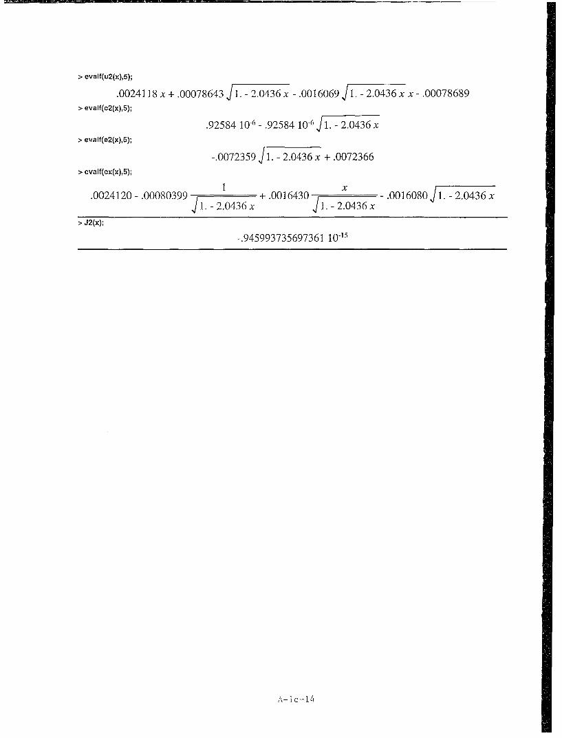
"> evalf(u2(x),5);
.0024118 x +.00078643 f1. - 2.0436 x - .0016069 f1. - 2.0436 x x - .00078689"> evalf(c2(x),5);
.92584 10-6 .92584 10-6 2.0436x
"> evalf(e2(x),5);
-.0072359 1. - 2.0436 x + .0072366"> evalf(ex(x),5);
1 x.0024120-.00080399 +.0016430 -. 0016080 1. -2.0436x
1.- 2.0436 x J 1.- 2.0436 x
"> J2(x);
-.945993735697361 10-15
A-Ic-14

1. MAPLE PROGRAM DIRECTORY AND FILE NAME:/afs/nd.edu/user4/jthomas5/Maple/Transport/lDSSsol#ld.ms
2. ORIGINATOR:Dr. James P. ThomasUniversity of Notre DameDepartment of Aerospace and Mechanical Engineering374 Fitzpatrick HallNotre Dame, IN 46556-5637(219) 631-9371
3. HISTORY:Written: June-1994Latest Revision: 13-Feb-1995
4. PROGRAM DESCRIPTION:One-dimensional, steady-state analysis of the fully coupled solute transport and trappingequations using "plane stress" constitutive equations for stress. The particular problemsolved is shown below:
'I/l I --- > x [m]Il'
x=O x=0.010
Deformation variable boundary conditions: u(O)=O, S(0.10)=0Concentration variable boundary conditions: J(O)=O, c(0.10)=le-7Reference concentration level: cO=0.0Trapping parameter: traps=19 (low trapping)
The equations used in the analysis are:
1. dJ/dx=O (steady-state diffusion equation)2. J=Ds*(Kl*c*de/dx-dc/dx) (mass flux)3. dS/dx=O (steady-state deformation equation with zero body forces)4. S=Bl*e-B2*c+B3 (axial stress)5. de/dx-K2*dc/dx=O (dilational strain gradient)6. e=Al*du/dx+A2*c-A3 (dilatational strain)
The constants used in the plane stress analysis are defined below:
Ds:=lattice diffusivity [m^2/sec]
Kl:=(Vs*K)/(R*T)Vs:= partial molar volume of solute [m^3/mol solute]K:= bulk modulus=Em/(3*(l-2*nu)) [N/m^2]Em:= Modulus of Elasticity [N/m^2]nu:= Poisson's ratio [1)R:= universal gas constant=8.31432 [J/mol-K]T:= temperature [K]
Bl:=3*KB2:=9*K*alpha*(l+traps)B3:=B2*cotraps:= Csr*Kr=trapping constant [1]Csr:= saturation trap concentration [I]Kr:= equilibrium trapping constant [13cO:= reference solute concentration [1]
K2:=3*alpha*(l+traps)alpha:= (rho*Vs)/(3*MWs)=solute concentration expansion coefficient [m/m/Delc]rho:= mass density of the solid [kg/m^3]MWs:= molecular weight of the solute [kg/mol]Delc:= c-c0 [I1
A-id-i

Al: =l-2*nuA2:=2*(l+nu)*alpha*(l+traps)A3 :=A2*cO
5. REQUIRED INPUTS:
Ds:=lattice diffusivity [m^2/sec]Vs:: partial molar volume of solute [m^3/mol solute]traps:= Csr*Kr=trapping constant [1]cO:= reference solute concentration [1]MWs':: molecular weight of the solute [kg/mol]
Em:= Modulus of Elasticity [Pa]nu:= Poisson's ratio [1]rho:= mass density of the solid [kg/m^3]
T:= temperature [K]
6. SYMBOLIC ANALYSIS:
"> restart;
"> Digits:=trunc(evalhf(Digits));
Digits:= 15
"> J:=Ds*(Kl*K2*c(x)-l)*diff(c(x),x);
J:= Ds (K1 K2 c(x) - 1) c(x)
"> deqn:=J=O;
deqn :=Ds (K1 K2 c(x) -1) c(x) 0
"> csoln:=dsolve(deqn,c(x),explicit);
1csoln := c(x) - , c(x) = C]K] K2
Note #1: There are apparently two "roots" to the solution for c(x) . Thefirst solution is obviously incorrect in that the concentrationthroughout the rod is defined in terms of the constants K1 and K2.The second solution is adopted as correct.
"> c2:=unapply(simplify(op(2,csoln[2])),x);
c2 :=x--- _C"> c2(x);
-C]
"> J2:=unapply(simplify(Ds*(Kl*K2*c2(x)-l)*diff(c2(x),x)));
J2 := 0"> J2(x);
0
Note #2: The above results show that the mass flux is identically zero, asit should be.
A-id-2

"> e2:=x->_C2;
e2 := x -- _C2"> e2(x);
_C2
"> ux2:=dsolve(A1 *diff(u(x),x)+A2*c2(x)-A3-e2(x)=o,u(x));
-x A2 _C] + x A3 + x _C2 + _C3 Alux2 :=u(x) -Al
"> u2:=unapply(simplify(op(2,ux2)),x);
-x A2 _C1 +xA3+x _C2+ _C3 A]u2 :=x --4
Al"> u2(x);
-xA2 _CI +xA3+x _C2+ _C3 A]
A]
"> S2:=x->simplify(Bl*e2(x)-B2*c2(x)+B3);
S2:= x --- simplify(BJ e2(x) - B2 c2(x) + B3)"> S2(x);
B] _C2 - B2 _CI + B3
Note #3: At this point, we will introduce expressions for the constants andthen simplify the results before quantifying the constants anddetermining the constants of integration.
"> K::(Em/(3*(1-2*nu)));
Em
3 -6v"> Iambda:=(Em*nu)/((l+nu)*(1-2*nu));
Em v
(1 +v)(1 -2v)"> mu:=EmI(2*(1+nu));
Em2+2v
"> alpha:=(rho*Vs)/(3*MWs);
1 p Vs
3 MWs"> K1 :=(Vs*K)/(R*T);
Vs EmK]
(3 -6v)RT"> K2::3*alpha*(1 +traps);
A-id-3

p Vs ( 1 + traps)K2 :MWs
"> KI*K2;
Vs2 Em p ( 1 + traps)
(3 - 6 v) R TMWs"> A1 :=(1-2*nu);
A]:= 1 -2 v"> A2:=2*(l +nu)*alpha*(l +traps);
2 (1 +v)p Vs(1 +traps)A2:=3 MWs
"> A3:=A2*cO;
2 (1 +v) p Vs(1 + traps) cOA3 := 3 MWs
"> B1:=3*K;
EmB]:= 3 -3-6v
"> B2:=9*K*alpha*(1 +traps);
B2 :=3 Em p Vs (1 + traps)
(3 - 6 v) MWs"> B3:=B2*cO;
Em p Vs ( 1 + traps) cO
(3 - 6 v) MWs
"> c2(x);
_C]
"> e2(x);
C2
"> u2(x);
2 2xI+v)p Vs(1+traps) Ci] 2x(I +v)p Vs(l +traps)cO- - +-±x _C23 MWs 3 MWs
+_c3 (I- 2 v))/(1- 2 v)
> S2(x);
Em(--C2 MWs + p Vs _C] + p Vs _C1 traps -p Vs cO - p Vs cO traps)
(-1 + 2 v) MWs
A-ld-4
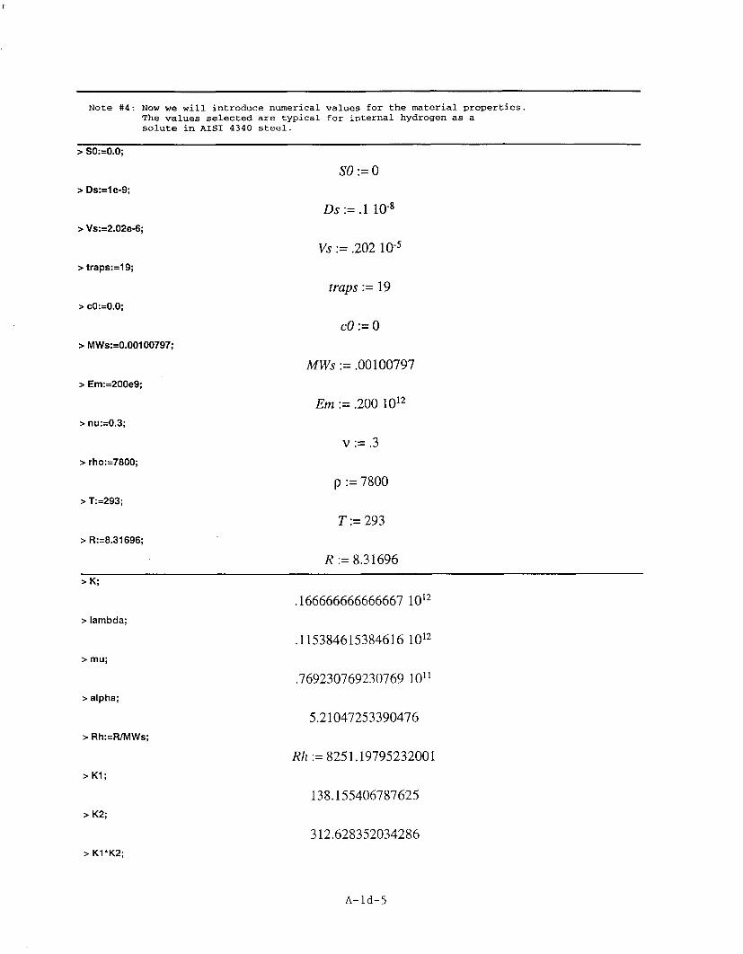
Note #4: Now we will introduce numerical values for the material properties.The values selected are typical for internal hydrogen as asolute in AISI 4340 steel.
"> SO:=0.0;
SO:= 0"> Ds:=Ie-9;
Ds:= .1 108
"> Vs:=2.02e-6;
Vs .202 10-5
"> traps:=19;
traps := 19"> cO:=0.0;
cO:=0"> MWs:=0.00100797;
MWs :=.00100797"> Em:=200e9;
Em :=.200 1012
"> nu:=0.3;
v :=.3"> rho:=7800;
p := 7800"> T:=293;
T:= 293"> R:=8.31696;
R := 8.31696> K;
.166666666666667 1012
"> lambda;
.115384615384616 1012
"> mu;
.769230769230769 1011"> alpha;
5.21047253390476"> Rh:=R/MWs;
Rh := 8251.19795232001"> K1;
138.155406787625"> K2;
312.628352034286"> KI*K2;
A-ld-5

43191.2971486416"> 1/(K1*K2);
.0000231528123954816"> Al;
.4"> A2;
270.944571763048"> A3;
0">B1;
.500000000000001 1012
"> B2;
.156314176017143 1015"> B3;
0
Note #6: Now let's solve for the integration constants: _Cl, -C2, and -C3, using theboundary data.
"> c2(x);
_C!"> C1:=le-7;
_CI := .1 10-6"> c2(x);
.1 10-6
"> u2(x);
-.0000677361429407620 x + 2.50000000000000 x _C2 + 1.00000000000000 _C3
"> S2(x);
.500000000000001 1012 _C2 -. 156314176017143 10'"> _C2:=solve(S2(0.1)=O.O,_C2);
C2 :=.0000312628352034285"> S2(x);
0"> u2(x);
.0000104209450678093 x + 1.00000000000000 _C3"> _C3:=solve(u2(O.O)=O,_C3);
_C3:= 0"> u2(x);
.0000104209450678093 x
A-id-6

"> e2(x);
.0000312628352034285"> pl :=plot(le6*e2(x/100),x=O..10,title='Dilatational Strain, e2(x) [ue]'):"> pi;
Dilatational Strain, e2(x) [ue]
32.2
32
31.8
31.6
31,4
31.2
31
30.8
30,6
30.4'
0 2 4 8 8 10x
"> p2:=plot(le6*u2(x/100),x=0..10,title='Displacement, u2(x) [urn]'):"> p2;
Displacement, u2(x) [urn]
0.6
0.4
0.2
0 2 4 6 8 10x
A-id-?
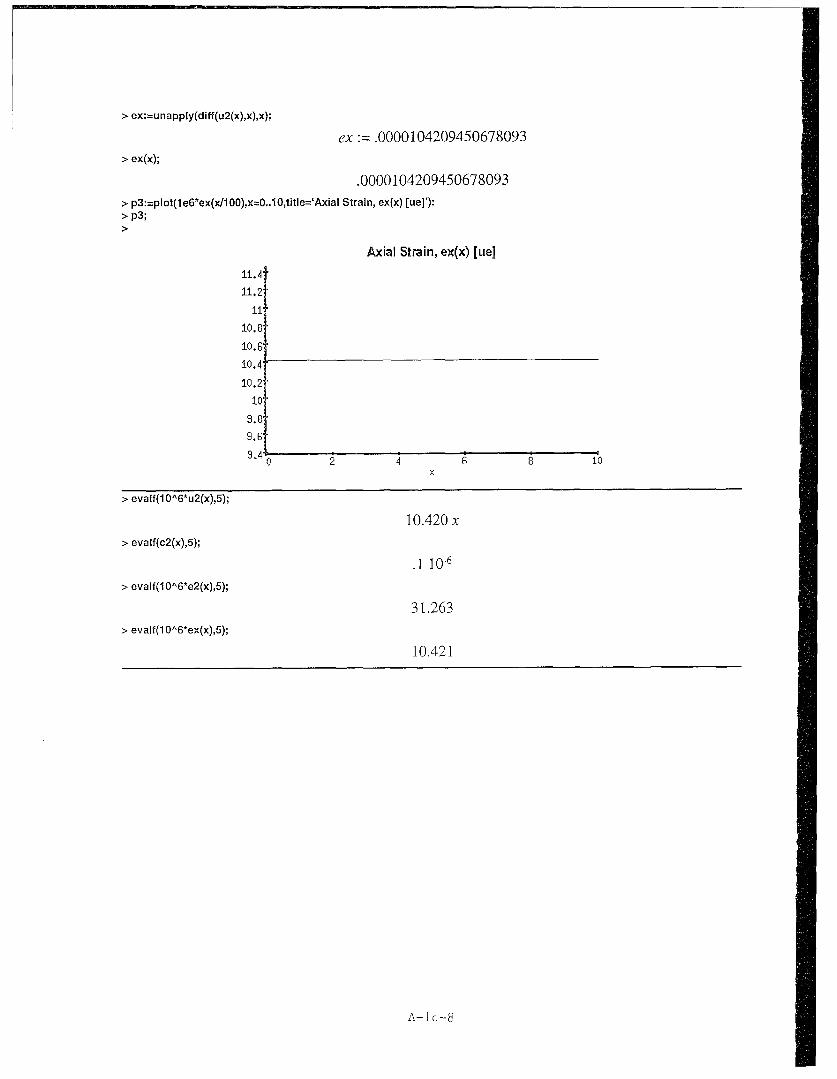
> ex:=unapply(diff(u2(x),x),x);
ex:=.0000104209450678093> ex(x);
.0000104209450678093> p3:=plot(1e6*ex(x/lOO),x=O..1O,title='Axial Strain, ex(x) [ue]'):> p3;
Axial Strain, ex(x) [ue]
11.4
11,2
A1
10.8
10,8
10.4
10.2
10
9.61
9402 4 8 8 10
"> evalf(1 0A6*u2(x),5);
10.420 x"> evalf(c2(x),5);
.1 10-6"> evalf(1lOAG6*e2(x),5);
3 1.263"> evalf(10A 6*ex(x),5);
10.42 1
A- Id-8
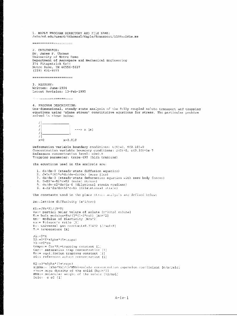
1. MAPLE PROGRAM DIRECTORY AND FILE NAME:/afs/nd.edu/user4/jthomas5/Maple/Transport/lDSSsol#le.ms
2. ORIGINATOR:Dr. James P. ThomasUniversity of Notre DameDepartment of Aerospace and Mechanical Engineering374 Fitzpatrick HallNotre Dame, IN 46556-5637(219) 631-9371
3. HISTORY:Written: June-1994Latest Revision: 13-Feb-1995
4. PROGRAM DESCRIPTION:One-dimensional, steady-state analysis of the fully coupled solute transport and trappingequations using "plane stress" constitutive equations for stress. The particular problemsolved is shown below:
S I --- > x [m]
Il'x=O x=0.010
Deformation variable boundary conditions: u(O)=O, S(0.10)=OConcentration variable boundary conditions: J(O)=O, c(0.10)=1e-7Reference concentration level: cO=0.0Trapping parameter: traps=499 (high trapping)
The equations used in the analysis are:
1. dJ/dx=O (steady-state diffusion equation)2. J=Ds*(Kl*c*de/dx-dc/dx) (mass flux)3. dS/dx=O (steady-state deformation equation with zero body forces)4. S=Bl*e-B2*c+B3 (axial stress)5. de/dx-K2*dc/dx=O (dilational strain gradient)6. e=Al*du/dx+A2*c-A3 (dilatational strain)
The constants used in the plane stress analysis are defined below:
Ds:=lattice diffusivity [m^2/sec]
Kl::(Vs*K)/(R*T)Vs:= partial molar volume of solute [m^3/mol solute]K:= bulk modulus=Em/(3*(l-2*nu)) [N/m^2]Em:= Modulus of Elasticity [N/m^2]nu:= Poisson's ratio [1]R:= universal gas constant=8.31432 [J/mol-K]T:= temperature [K]
Bl:=3*KB2:=9*K*alpha*(l+traps)B3 : =B2*cotraps:= Csr*Kr=trapping constant [1]Csr:= saturation trap concentration [1]Kr:= equilibrium trapping constant [1]cO:= reference solute concentration [1)
K2:=3*alpha*(l+traps)alpha:= (rho*Vs)/(3*MWs)=solute concentration expansion coefficient [m/m/Delc]rho:= mass density of the solid [kg/m^3]MWs:= molecular weight of the solute (kg/mol]Delc:= c-cO [11
A-le-1

Al: =l-2*nuA2 ::2* (l+nu) *alpha* (l+traps)A3 :=A2*cO
5. REQUIRED INPUTS:
Ds::lattice diffusivity [m^2/sec]Vs:= partial molar volume of solute [m^3/mol solute]traps:= Csr*Kr=trapping constant [1]cO:= reference solute concentration [1]MWs!= molecular weight of the solute [kg/moll
Em:= Modulus of Elasticity [Pa]nu:= Poisson's ratio [1]rho:= mass density of the solid [kg/m^3]
T:= temperature [K]
6. SYMBOLIC ANALYSIS:
"> Digits:=tr unc(evalhf(Digits));
Digits:= 15"> J:=Ds*(Kl*K2*c(x)-l)*diff(c(x),x);
J:=Ds(K] K2c(x)- 1) c(x)
"> deqn:=J=O;
deqn :=Ds(K1K2c(x)- 1) -c(x) = 0
"> csoln:=dsolve(deqnc(x),explicit);
1csoln c(x) - , c(x) = C]
Note #1: There are apparently two "roots" to the solution for c(x) . Thefirst solution is obviously incorrect in that the concentrationthroughout the rod is defined in terms of the constants Kl and K2.The second solution is adopted as correct.
"> c2:=unapply(simplify(op(2,csoln[2])),x);
c2 := x --> _C1"> c2(x);
C]
"> J2:=unapply(simpIify(Ds*(Kl*K2*c2(x)-l)*diff(c2(x),x)));
J2: 0"> J2(x);
0
Note #2: The above results show that the mass flux is identically zero, asit should be.
A-le-2
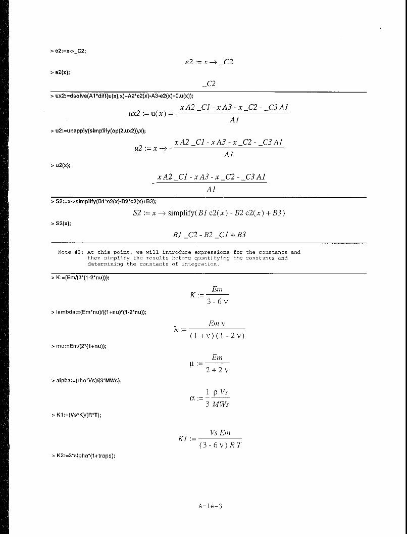
">e2:=x->-C2;
e2 := x-> _C2"> e2(x);
-C2
"> ux2:=dsolve(A1 *diff(u(x),x)+A2*c2(x)-A3..e2(x)=0,u(x));
ux2= ux) xA2 -C]-xA3 -x C2 -C3 A]
Al"> u2:=unapply(simplify(op(2,ux2)),x);
u2: x xA2 -C -xA3 -x _C2- C3 Al
A]"> u2(x);
xA2 C] -xA3 -x _C2- -C3A]
A]
"> S2:=x->simplify(B1 *e2(x)-B2*c2(x)+B3);
S2 := x --ý simplify(B] e2(x) - B2 c2(x) + B3)"> S2(x);
B] _C2 -B2 _C]±+B3
Note #3: At this point, we will introduce expressions for the constants andthen simplify the results hefore quantifying the constants anddeternining the constants of integration.
EmK.=
"> Iambda:=(Em*nu)/((1+nu)*(1-2*nu));
Em v
(1 +v) (I - 2v)"> mu:=EmIC2*(1+nu));
Em
2±+2 v"> alpha:=(rho*Vs)I(3*MWs);
I 1p Vs
3 MWs"> Ki :=(Vs*K)I(R*T);
Vs EmnK]:
(3 -6 v) R T"> K2:=3*alpha*(l +traps);
A-Ie-3

K2 := p Vs ( 1 + traps)
MWs
"> Kl*K2;
Vs 2 Em p (1 + traps)
(3- 6v) R TMWs"> A1 :=(1-2*nu);
A]:= 1 -2 v"> A2:=2*(l +nu)*alpha*(l +traps);
2 (1 +v)p Vs(l +traps)A2:=3 MWs
"> A3:=A2*cO;
2 (1+v)pVs(I+traps)cOA3 :=- 3 MWs
"> B1:=3*K;
EmB]:= 3 -
3 -6v"> B2:=9*K*alpha*(l+traps);
Em p Vs ( 1 + traps)B2 :3 .(3 - 6 v) MWs
"> B3:=B2*cO;
Em p Vs ( 1 + traps) cOB3 3(3 - 6 v) MWs
"> c2(x);
-C]
" e2(x);
_C2
"> collect(u2(x),x);
2(1+ v) pVs(1+traps) C 2(1 +v)p Vs(I+traps)cO C(+vp MWs 3 MWs -C x
33 + C3
1 -2v
"> S2(x);
Em (--C2 MWs + p Vs _Cl + p Vs _C] traps - p Vs cO - p Vs cO traps)
(-1 + 2 v) MWs
A-le-4
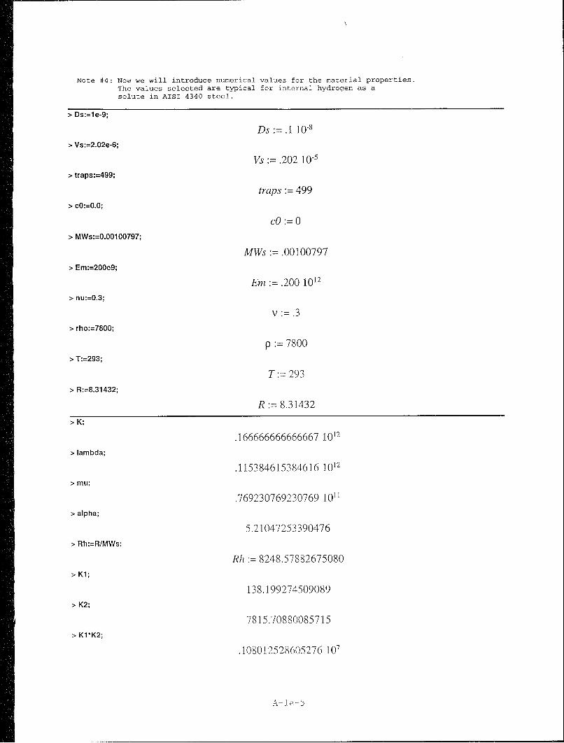
Note #4: Now we will introduce numerical values for the material properties.The values selected are typical for internal hydrogen as asolute in AISI 4340 steel.
"> Ds:=le-9;
Ds: .1 10-1"> Vs:=2.02e-6;
Vs :=.202 10'"> traps:=499;
traps := 499
"> cO:=O.O;
cO:= 0"> MWs:=O.00100797;
MWs :=.00100797
"> Em:=200e9;
Em :=.200 1012
"> nu:=0.3;
v :=.3"> rho:=7800;
p := 7800
"> T:=293;
T:= 293
"> R:=8.31432;
R:= 8.31432
> K;
.166666666666667 1012
"> lambda;
.115384615384616 1012
"> mu;
.769230769230769 1011"> alpha;
5.21047253390476"> Rh:=R/MWs;
Rh := 8248.57882675080"> K1;
138.199274509089"> K2;
7815.70880085715"> KI*K2;
.108012528605276 107
A-le-5

"> 1/(K1*K2);
.925818525788271 10-6
"> Al;.4
"> A2;
6773.61429407620"> A3;
0"> Bi;
.500000000000001 1012
"> B2;
.390785440042860 1016
"> B3;
0
Note #6: Now let's solve for the integration constants: CI, _C2, and C3, using theboundary data.
"> c2(x);
C]"> _Cl:=l e-7;
C] := .1 10-6
"> c2(x);
.1 10.6
"> u2(x);
-.00169340357351905 x + 2.50000000000000 x _C2 + 1.00000000000000 _C3"> S2(x);
.500000000000001 1012 _C2- .390785440042860 109"> _C2:=solve(S2(0.1)=O.O,_C2);
C2 :=.000781570880085718"> S2(x);
0"> u2(x);
.000260523626695245 x + 1.00000000000000 _C3"> C3:=solve(u2(O.O)=O,-C3);
C3 :=0"> u2(x);
.000260523626695245 x"> e2(x);
.000781570880085718
A-le-6

1. MAPLE PROGRAM DIRECTORY AND FILE NAME:/afs/nd.edu/user4/jthomas5/Maple/Transport/lDSSsol#2a.ms
2. ORIGINATOR:Dr. James P. ThomasUniversity of Notre DameDepartment of Aerospace and Mechanical Engineering374 Fitzpatrick HallNotre Dame, IN 46556-5637(219) 631-9371
3. HISTORY:Written: June-1994Latest Revision: 13-Feb-1995
4. PROGRAM DESCRIPTION:One-dimensional, steady-state analysis of the fully coupled solute transport and trappingequations using "plane stress" constitutive equations for stress. The particular problemsolved is shown below:
--- > x [m]
/l I
x=0 x=0.010
Deformation variable boundary conditions: u(O)=O, u(0.10)=OConcentration variable boundary conditions: c(O)=O, c(0.10)=le-6Reference concentration level: cQ=0.0Trapping parameter: traps=19 (low trapping)
The equations used in the analysis are:
1. dJ/dx:O (steady-state diffusion equation)2. J=Ds*(Kl*c*de/dx-dc/dx) (mass flux)3. dS/dx=O (steady-state deformation equation with zero body forces)4. S=Bl*e-B2*c+B3 (axial stress)5. de/dx-K2*dc/dx=O (dilational strain gradient)6. e=Al*du/dx+A2*c-A3 (dilatational strain)
The constants used in the plane stress analysis are defined below:
Ds:=lattice diffusivity [m^2/sec3
Kl:=(Vs*K)/(R*T)Vs:= partial molar volume of solute [m^3/mol solute]K:= bulk modulus=Em/(3*(l-2*nu)) [N/m^2]Em:= Modulus of Elasticity IN/m^2]nu:= Poisson's ratio [1]R:= universal gas constant=8.31432 [J/mol-K]T:= temperature [K]
Bl:=3*KB2:=9*K*alpha*(l+traps)B3:=B2*cotraps:= Csr*Kr=trapping constant [13Csr:= saturation trap concentration [1)Kr:= equilibrium trapping constant [1)cO:= reference solute concentration [1]
K2:=3*alpha*(l+traps)alpha:= (rho*Vs)/(3*MWs)=solute concentration expansion coefficient [m/m/Delc]rho:= mass density of the solid [kg/m^3]MWs:= molecular weight of the solute [kg/mol]Delc:= c-c0 [1]
A-2a-i

Al: =1-2 *nu
A2:=2*(l+nu)*alpha*(l+traps)A3 : =A2 *cO
5. REQUIRED INPUTS:
Ds:=lattice diffusivity [m^2/sec]Vs:: partial molar volume of solute [m^3/mol solute]traps:= Csr*Kr=trapping constant [1]cO:= reference solute concentration [1]MWs:= molecular weight of the solute [kg/mol]
Em:= Modulus of Elasticity [Pa]nu:= Poisson's ratio [1]rho:= mass density of the solid [kg/m^3]
T:= temperature [K]
6. SYMBOLIC ANALYSIS:
"> Digits:=tru nc(evalhf(Digits));
Digits 15
"> J:=Ds*(Kl*K2*c(x)-l)*diff(c(x),x);
J:=Ds(KI K2 c(x) -1) -c(x)
"> deqn:=diff(J,x)=O;
deqn :Ds K] K2 -c(x) + Ds (K] K2 c(x) - 1) ( 2c(x) 0
"> csoIn:=dsolve(deqn,c(x),expIicit);
esi I jI 1 +2K1K2 Clx+2K1K2 C] C2IC1 1 - -
csoln := c(x) KI-KK] K2
C + 1+2K]K2 Clx+2K]K2 C1 C2
- • _ -C1 _I K C 1K] K2
Note 41: There are apparently two "roo-s" to the solution for c(x) . Theboundary conditions will be used to select the proper one.
"> cl:=unapply(simplify(op(2,csoln[1])),x);
x I KI K2 C] x + 2 K1K2 C] _C2cl : x -->_
KI K2"> cl (x);
1 + J1 + 2 K] K2_C1 x + 2 KI K2 C1 _C2
KI K2
A-2a-2

"> c2:=unapply(simplify(op(2,csoln[2])),x);
c2:= -ý--1+j1+2K]K2 Clx+2K1K2-Cl C2
K] K2"> c2(x);
-1+J1+2K]K2 Clx+2K]K2-Cl-C2
K] K2
"> Ji :=unapply(simplify(Ds*(K1*K2*cl(x)-1)*diff(cl(x),x),x));
J]:= )-4Ds C1> J1(x):
Ds C1"> J2:=unapply(simplify(Ds*(K1 K2*c2(x)-1 )*diff(c2(x),x)));
J2:=( )Ds C]"> J2(x);
Ds C]
Note #2: The above results show that both mass flux solutions are identicaland equal to Ds*-C1 where _C1 is a constant of integration!
"> exi :=dsolve(diff(e(x),x)-K2*diff(c1(x),x)=O,e(x));
exl=ex)J 1+2K1K2 Clx+2K1K2 Cl- C2+ C3KJ
"> el :=unapply(simplify(op(2,exl)),x);
el:=I 1j+2K1K2 Clx±2K]K2 C] C2+ C3KJ
K]"> el (x);
J 1+2K1K2 C~x+2K]K2 C1 -C2± C3K]
K]"> ex2:=dsolve(diff(e(x),x)-K2*diff(c2(x),x)0O,e(x));
ex2=eX)-j1+2K]K2 C'x+2K]K2 C] C2+ C3K1
"> e2:=unapply(simplify(op(2,ex2)),x);
-j1+2K]K2 Clx+2K]K2 C] C2± C3KJe2 := xK]
"> e2(x);
1j+ 2 K]K2 -C x + 2 KK2 -CI C2 + -C3 K]
K]
A-2a-3

> uxi :=dsolve(Al~diff(u(x),x)+A2*cl(x)-A3..el(x)=O,u(x));
UXl :=u(x) = 1(-3 A2 x KJK2 _CJ -A2 %0/1 -2 %701A2 KJK2 -Cl x3
-2/0 %A2 KJK2 Cl _C2 + 3A3 XK12 K22 _CJ + 001 K2 +2J To 1K2 2 K Cl x
+ 2 %1lolK2 2 K1 Cl _C2 +3 _ C3 XKJ2K22 _CJ +3 _C4 AJ KJ 2 K22 -_ol)/(A]K12
K22 _C1)
%1:= 1+ 2 K1K2 _Cl x+ 2 K1K2 -Cl _C2> ul :=unapply(simplify(op(2,uxl )),x);
ul:= x -4(-3 A2 xK]K2 -CJ-A2J1l+ 2 K1K2 _Cl x+ 2 K1K2 -Cl _C23
-2j1l+ 2 KK2 _Cl x+ 2 KJK2 -Cl _C2 A2 KJK2 -Cl x
- 2J1l+ 2 KK2 _Cl x+ 2 K1K2 -Cl _C2 A2 KJK2 -Cl _C2 +3 A3 XK12 K22 -Cl
+j 1 + 2 KK2 _Cl x+ 2 K1K2 -Cl _C2 K2
*+2jl+ 2 K1K2 _Cl x +2 K1K2 -Cl _C2 K22 K -Cl x
*+2J11+ 2 K1K2 _Cl x +2 K1K2 -Cl _C2 K2 2 K -Cl _C2 +3 _C3 xK12 K2 2 -Cl
+ 3 -C4 AlK1 2 K2 2 -C ),/(A]JK12K22 _Ci)
> ul(x);
±(-3 A2 x KlK2 _CJ -A2 %0/1 -2 %I1 A2 KJK2 _Cl x -2 %o1 A2 KJK2 -Cl _C23
*+3A3 xK12 K2 2 _ Cl±+'l %1K2 +2 %1 K2 2 K _Cl x +2 %OO1 K22 K1 _C] _C2
+ 3 _C3 XK1 2 K22 _CJ +3 _C4 Al K]2K22 -CJ )/(A1 K12 K22 _Cl)
%1:=1I+ 2 K1K2 -Cl x+ 2 KK2 Cl -C2> ux2:=dsolve(A1 *djff(u(x),x)+A2*c2(x)-A3-e2(x)=O~u(x));
ux2:= u(x)=-(--3A2 x KlK2 _CJ +A2 %ll+ 2 %1otA2 KJK2 -Cl x3
+ 2 %1l-IA2 KJK2 Cl _C2 +3 A3 xK12 K22 Cl-/ %1K2 -2 %1l IK2 2 K1 Cl x
- 2 %o-1 K22 K1 Cl _C2 +3 _C3 xK12 K22 _Cl +3 _C4Al1K12 K22 _ C )/(A]K12
K22 _C1)
%1:= 1+ 2 KK2 _Cl x+ 2KlK2 -Cl _C2
A- 2 a-4

> u2:=unapply(simplify(op(2,ux2)),x);
u2:=x--4- -3A2xKIK2 C] +A2J +2 K1K2Cl x_ +2KI K2_CI _C23
+2j 1 + 2 K1K2 _Cl x + 2 KI K2 CI _C2 A2 K1K2 C1 x
+ 2 J 1 + 2 K1 K2 _C1 x + 2 K1 K2 _CI _C2 A2 KJ K2 _CI _C2 + 3 A3 x K12 K22 _C1
-J1+ 2 K1 K2 _CI x + 2 KJ K2 _CI _C2 K2
- 2 J1 + 2 K1 K2 _Cl x + 2 Ki K2 _C] _C2 K22 K1 _CI x
- 2 J1 + 2 K1 K2 _C1 x + 2 KJ K2 _Cl _C2 K22 KJ _C1 _C2 + 3 _C3 x K12 K22 _C1
+ 3 _C4 AJ K12 K22 _C1)/(A1 K12 K22 _C])"> u2(x);
1(-3 A2x KJ K2 Ci + A2 %ol +2 F%1 A2 K1 K2 _Clx +2 o 1A2 K1 K2 C1 _C2
3
+3A3xK12 K22 _C - %1K2-2 %1K22 K1 Cl x - 2 [-%o1K22 K1 C1_C2
+ 3 _C3 x K12 K22 _Ci + 3 _C4 A] K12 K22 _C1 )/(AJ K12 K22 _CJ)
%1:= 1 + 2 K1 K2 _Cl x + 2 K] K2 _Ci _C2
"> Si :=x->simplify(Bl *el (x)-B2*cl (x)+B3);
S1 := x -- simplify(B] el(x) - B2 cl(x) + B3)
"> S1(x);
(B1 K2 J 1 + 2 Ki K2 _Ci x + 2 K1 K2 _Ci _C2 + B] K2 _C3 Kl - B2
- B2 j 1 + 2 K1 K2 _C1 x + 2 K] K2 _CI _C2 + B3 K1 K2)/(K1 K2)"> S2:=x->simplify(B1 *e2(x)-B2*c2(x)+B3);
S2 x -- simplify(B! e2(x) - B2 c2(x) + B3)
"> S2(x);
(-B1 K2 j1 + 2 K1 K2 _C] x + 2 K] K2 _C] _C2 + B] K2 _C3 Kl- B2
+ B2 J 1 + 2 K1 K2 _C1 x + 2 K] K2 _C] _C2 + B3 K1 K2)/(K K2)
Note #3: At this point, we will introduce expressions for the constants andthen simplify the results before quantifying the constants anddetermining the constants of integration.
"> K:=(Em/(3*(1-2*nu)));
Ein= ~K:= -
3 -6v"> Iambda:=(Em*nu)/((1+nu)*(1-2*nu));
SEm v
(1+ v)(1 -2v)
A-2a-5

"> mu:=EmI(2*(1+nu));
Em
2 2+2v
"> alpha:=(rho*Vs)/(3*MWs);
1 p Vs
3 MWs
"> K1 :=(Vs*K)/(R*T);
Vs EmK]
(3 -6v)R T
"> K2:=3*alpha*(l +traps);
p Vs ( 1 + traps)K2 :MWs
"> K1*K2;
Vs2 Em p (1 + traps)
(3 - 6 v) R TMWs"> A1 :=(1-2*nu);
A]:= 1 -2v"> A2:=2*(l+nu)*alpha*(l+traps);
2 (1 +v) p Vs(1 +traps)A2:=3 MWs
"> A3:=A2*cO;
2 (1 +v)p Vs(1 +traps)cOA 3 := 3 MWs
" BI:=3*K;
EntBl:=3--3 -B6:v
"> B2:=9*K*alpha*(l +traps);
Em p Vs (1 + traps)B2 :3(3 - 6 v) MWs
"> B3:=B2*cO;
Em p Vs (1 + traps) cOB3:=3(3 - 6 v) MWs
A-2a-6
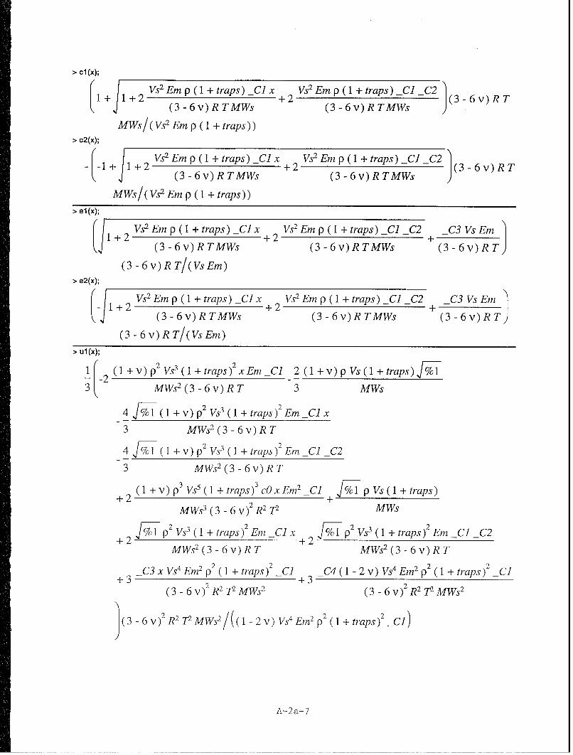
> cl (x);
S+ Vs2 Emp(1+traps) C]x Vs2 Emp(1 + traps) C] C2 )
• (3 - 6 v) R TMWs (3 - 6 v) R TMWs
MWs/(Vs2 Em p (1 + traps))> c2(x);
S + Vs2 Emp(1+traps) Clx Vs2 Emp(l+traps) C1 C2
+2 (3 - 6 v) R TMWs (3 - 6 v) R TMWs
MWs/(VS2 Em p ( 1 + traps))
> el (x);
VS2 Em p (1 + traps) C1 x Vs2 Em p ( 1 + traps) C1 C2 C3 Vs EmK1+2 - +2-- +-(3 - 6v) R TMWs (3 - 6v) R TMWs (3 - 6v) R T
(3 - 6 v) R T/(Vs Em)"> e2(x);
VS2 Em p ( 1 + traps) CI x Vs 2 Em p (1 + traps) C1 C2 C3 Vs Em-K1 2 - ±2 -- + -(3 - 6v) R TMWs (3 - 6v) R TMWs (3 - 6v) R T
(3 - 6 v) R T/(Vs Em)
"> ul(x);
Sx(1V)pVs3 (1traps)xEmCl 2(1+v)pVs(1+traps) %1
3 MWs2 (3 - 6 v) R T 3 MWs
4 O 1 (1 + v) p2 Vs3 (1 + traps)2 Em _C1 x
3 MWs2 (3 - 6 v) R T4 %1 (1 +v) P2 Vs3 (1 traps)2 Em C2
3 MWs 2(3 - 6 v) R T
+2 (1+v)p 3 Vs5(+traps)3 cOxEm2 Cl +%l pVs(l+traps)+
MWs3 (3 - 6 v) 2 R2 V MWs
p p 2 Vs 3 (1 + traps)2 Em Cl x ±2•%1 p 2 Vs3 (1 + traps)2 Em Cl C2+2- +2 T
MWs2 (3 - 6v) R T MWs2 (3 - 6v)R T
C3 X Vs4 Em2 p2 ( 1 + traps )2 _C+ C4 (1 - 2 v) Vs4 Em2 p2 (1 + traps)2 _C1±3 -+3-(3 - 6 v) 2 R2 V MWs2 (3 - 6 v) 2 R 2 ViMWs2
(3 V)2 R2MWS2 /((2 v) Vs4 Em2p2 (1 + traps )2 Cl
A-2a-7
Vs2 Em p (1 + traps) _C1 x Vs2 Em p ( 1 + traps) _C1 -C2%1 :-1 +2 +2_(3 - 6 v) R TMWs (3 - 6 v) R TMWs
A-2a-8

> u2(x);
1-2 (1+V)2Vs3(1+traps)2x2Em C1 2 (1+v)pVs(l+traps) %1
MWS2 (3-6v)RT 3 MWs
4 %I (1+V)p 2 VS(1+traps)2 EM ClX
3 MW (3 - 6 v) R T
4 /1 ( 1 + v) p2 Vs3 (1 + traps) 2 Em _C C2
3 MWs2 (3- 6v) R T1+ v) P 3Vs5 ( 1 + traps)3 cOxEm2 _C1 C p2Vs(+traps)+ /
3(MWs1 (3 - 6 v) 2R 2T_ _
+2 ( 1 p2 )9 VS3 ( 1+ traps)2 EmCO x E2_C 1_0 1%o p2 Vs (1l + traps)2E CI 2MWs 3(3-6v) R2T MWs
22 2 (3 - 6 v2 T- f-ol92V3 1+trps2Em C1x %1o p2Vs ( 1+ traps)2 Em C1 C2-2- 2- -
MWs2 (3- 6v) R T MWs2 (3 - 6V) R T
+3C3XVS4 Em 2 p 2 (1 + traps) C1 C4 ( 1 -2 v) s 4 Em2 p2 (1 +traps)C( 3 -6 v) 2 R27T2MWs2 (3 -6 V)2 R2 Ji,2MWs2
(3-6 v)Z2R27i2MWs2/((1- 2V)Vs4 EmZ p2 (1 + traps)2 _Cl)
Vs2 Em p( 1 +traps) C1 x Vs2 Em p( 1 +traps)jC1 _C2%1 := 1 +2 +2
(3- 6v) R TMWs (3 - 6 v) R TMWs
"> S1 (x);
- (MWs _C3 Vs Em - 3 R TMWs + 6 R TMWs v + Em p Vs 2 cO + Em p Vs 2 cO traps)/(
(-1 + 2 v) Vs MWs)
"> S2(x);
- (MWs _C3 Vs Em - 3 R TMWs + 6 R TMWs v + Em p Vs2 cO + Em p VS2 cO traps)/(
(-1 +2v) VsMWs)"> S1(x)-S2(x);
0
Note #4: The stresses are same for each solution root, and do not depend onthe position x! The stresses are therefore constant throughout thebody. We define a new stress function, Sx.
"> Sx::S2(x);
Sx:= - (MWs _C3 Vs Em - 3 R TMWs + 6 R TMWs v + Em p Vs2 cO +Em p Vs2 cO traps)l(
(-1 +2v) VsMWs)
A-2a-9

Note #5: Now we will introduce numerical values for the material properties.The values selected are typical for internal hydrogen as asolute in AISI 4340 steel.
"> Ds:=le-9;
Ds:= .1 10-8"> Vs:=2.02e-6;
Vs :=.202 10-"> traps:=19;
traps := 19
"> cO:=0.0;
cO:= 0"> MWs:=0.00100797;
MWs :=.00100797"> Em:=200e9;
Em := .200 1012
"> nu:=0.3;
v := .3"> rho:=7800;
p := 7800"> T:=293;
T:= 293"> R:=8.31432;
R := 8.31432
> K;
.166666666666667 1012
"> lambda;
.115384615384616 1012
"> mu;
.769230769230769 1011"> alpha;
5.21047253390476"> Rh:=R/MWs;
Rh:= 8248.57882675080"> KI;
138.199274509089"> K2;
312.628352034286"> K1*K2;
43205.0114421104
A-2a-10

"> 1/(K1*K2);
.0000231454631447068"> Al;
.4"> A2;
270.944571763048"> A3;
0"> Bi;
.500000000000001 1012
"> B2;
.156314176017143 1015
"> B3;
0
Note #6: Now let's solve for the integration constants: _CI, _C2, _C3, and C4,using the boundary data.
"> cl (x);
.0000231454631447068 + .0000231454631447068
S_1 + 86410.0228842208 _C] x + 86410.0228842208 _Cl _C2"> c2(x);
.0000231454631447068 - .0000231454631447068
SI + 86410.0228842208 _CI x + 86410.0228842208 _Cl _C2"> evalf(cl (x),5);
.000023146+ .000023146 J 1. + 86408. Cl x + 86408. _C1 _C2"> evalf(c2(x),5);
.000023146- .000023146 J 1. + 86408. C] x + 86408. _CI C2"> eqnsetl :={0=cl (0),1 e-6=cl (0.10)};
eqnsetl := t. 1 10-5 = .0000231454631447068 + .0000231454631447068
1 1+ 8641.00228842208 _Cl + 86410.0228842208 _CI _C2,0 =
.0000231454631447068 + .0000231454631447068 1 1 + 86410.0228842208 Cl _C2 }"> varsetl :={Cl ,C2};
varset] Cl, -C2}"> soinsetl:=solve(eqnsetl,varsetl);
solnset]"> eqnset2:={O=c2(0),le-6=c2(0.10)};
eqnset2 := { 0 =
.0000231454631447068 - .0000231454631447068 J I + 86410.0228842208 _Cl _C2,
A-2a-1 1

.1 105 =.0000231454631447068
-. 0000231454631447068 J 1 + 8641.00228842208 _C] + 86410.0228842208 _C1 _C2}
"> varset2:={_C1,,C2};
varset2 -C], -C2"> solnset2:=solve(eqnset2,varset2);
solnset2 { C2 = 0, -CI = -.978397494278943 10- }"> assign(soinset2);
Note #7: The solution cl(x) is not capable of satisfying the boundaryconditions, as evidenced by the lack of solution for the givenboundary conditions. The concentration function c2(x) is thecorrect solution in this case!
"> c2(x);
.0000231454631447068 - .0000231454631447068 J 1 -_.845433498705078 x"> pl:=plot(le6*c2(x/lOO),x=O..1O,title='Concentration, c2(x) [ppm]'):
"> P1;
Concentration, c2(x) [ppm]
0.6
0,4i
0.2"
2 4 6 8 10x
"> p2:=plot(1 e9*(c2(0)+((c2(0.1 O)-c2(O))/O.l O)*x/1 O0-c2(x/1 00)),x=O..1 O,title='Concentration Difference [ppb]'):"> p2;>
Concentration Difference [ppb]
5"
4'
3'
2"
0 2 4 6 8 10x
A-2a-12
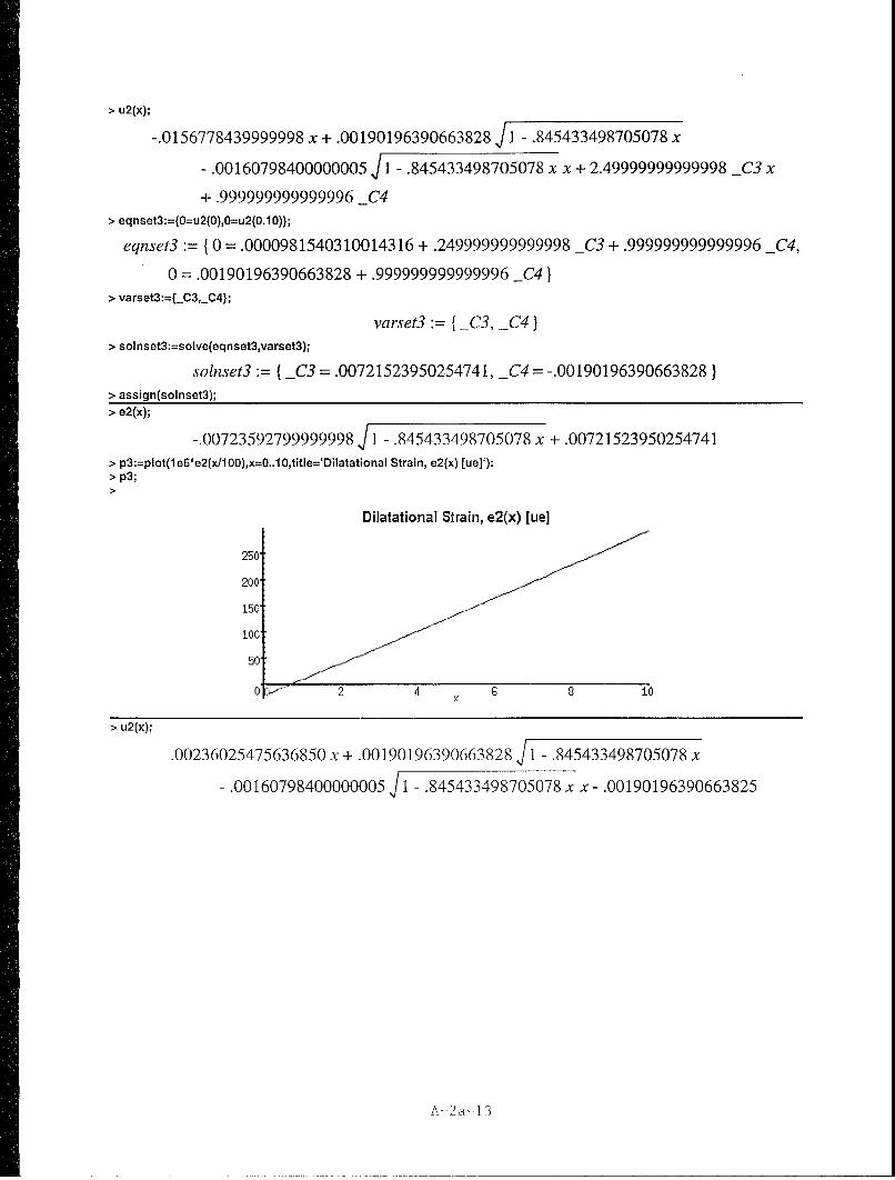
"> u2(x);
-.0 156778439999998 x + .00190196390663828 J1 - .845433498705078 x
- .00160798400000005 j 1 -_.845433498705078 x x + 2.49999999999998 _C3 x
+ .999999999999996 _C4"> eqnset3:={0=u2(0),0=u2(0.10)};
eqnset3 :={ 0 = .0000981540310014316 + .249999999999998 _C3 + .999999999999996 _C4,
0 = .00190196390663828 + .999999999999996 _C4 }"> varset3:={_C3,_C4};
varset3 -C3, C4 }"> solnset3:=solve(eqnset3,varset3);
solnset3:= { _C3 = .00721523950254741, _C4 = -.00190196390663828 }"> assign(solnset3);
"> e2(x);
-.00723592799999998 j 1 - .845433498705078 x + .00721523950254741S>" pa:=plot(le6*e2(x/100),x=0..10,title='DilatationaI Strain, e2(x) [ue]'):
"> p3;
Dilatational Strain, e2(x) [ue]
250
200
150
100
50
0[ 2 4 6 8 10x
> u2(x);
.00236025475636850x + .00190196390663828 Ji -_.845433498705078 x
- .00160798400000005 J1 -_.845433498705078 xx - .00190196390663825
A-2a-l3

"> p4:=plot(1e6*u2(x/lOO),x0O..1O,title='Displacernent, u2(x) [urn]):"> p4;
02 Displa~erneii, u2(ý) [urn] 8 i
-0.4
-0.6
-0,8
-1
-1.2
"> ex:=unapply(diff (u2(x),x),x);
ex: x -> .00236025475636850 - .000803991999999990 J 1_-_.845433498705078 x
+ .000679721769490914 -
I 1_-_.845433498705078 x
-.00160798400000005 J -_.845433498705078 x"> p5:=plot(l e6*ex(x/l OO),x=O..1 O,title='AxiaI Strain, ex(x) [ue]'):"> p5;
Axial Strain, ex(x) [ue]
40"
20'
2 4 6 8 10
-20
-40-
A-2a-14

> Sx;
-.103442487262901 108
> J2(x);
-.978397494278943 10-14
> evalf(u2(x),5);
.0023588x+.0019015fl. -. 84542x -. 0016072j 1.-.84542x x-.0019021> evalf(c2(x),5);
.000023146 -. 000023146 J1. - .84542 x> evalf(e2(x),5);
-.0072359 1 1. - .84542x + .0072152> evalf(ex(x),5);
1 x.0023603-.00080399 +.00067972 -. 0016080 1. - .84543 x
,1.- .84543 x J1.-.84543 x
A-2a-15

1. MAPLE PROGRAM DIRECTORY AND FILE NAME:/afs/nd.edu/user4/jthomas5/Maple/Transport/lDSSsol#2b.ms
2. ORIGINATOR:Dr. James P. ThomasUniversity of Notre DameDepartment of Aerospace and Mechanical Engineering374 Fitzpatrick HallNotre Dame, IN 46556-5637(219) 631-9371
3. HISTORY:Written: June-1994Latest Revision: 13-Feb-1995
4. PROGRAM DESCRIPTION:One-dimensional, steady-state analysis of the fully coupled solute transport and trappingequations using "plane stress" constitutive equations for stress. The particular problemsolved is shown below:
'III/I _ _ _ _- - -> X [m ]
x=O x=0.010
Deformation variable boundary conditions: u(O)=O, u(0.10)=OConcentration variable boundary conditions: c(O)=O, c(0.10)=le-7Reference concentration level: cO=0.0Trapping parameter: traps=19 (low trapping)
The equations used in the analysis are:
1. dJ/dx=O (steady-state diffusion equation)2. J=Ds*(Kl*c*de/dx-dc/dx) (mass flux)3. dS/dx=O (steady-state deformation equation with zero body forces)4. S=Bl*e-B2*c+B3 (axial stress)5. de/dx-K2*dc/dx=O (dilational strain gradient)6. e=Al*du/dx+A2*c-A3 (dilatational strain)
The constants used in the plane stress analysis are defined below:
Ds::lattice diffusivity [m^2/sec]
Kl::(Vs*K)/(R*T)Vs:= partial molar volume of solute [m^3/mol solute]K:= bulk modulus=Em/(3*(l-2*nu)) [N/m^2]Em:= Modulus of Elasticity [N/m^2]nu:= Poisson's ratio [1]R:- universal gas constant=8.31432 [J/mol-K]T:= temperature [K]
Bl:=3*KB2:=9*K*alpha*(l+traps)B3:=B2*cotraps:= Csr*Kr=trapping constant [1]Csr:= saturation trap concentration [1]Kr:= equilibrium trapping constant [1]cO:= reference solute concentration [1]
K2::3*alpha*(l+traps)alpha:= (rho*Vs) / (3*MWs)=solute concentration expansion coefficient [m/m/Delc]rho:= mass density of the solid [kg/m^3]MWs:= molecular weight of the solute [kg/mol]Delc:= c-cO [1]
A-2b-1
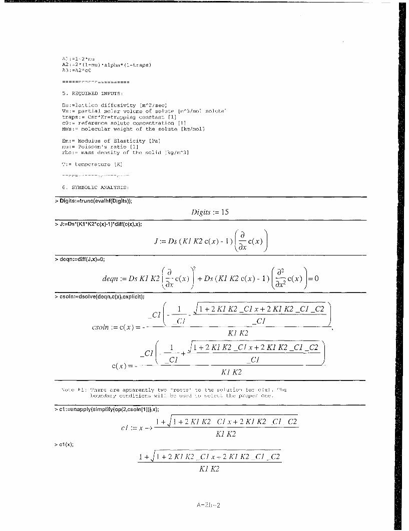
Al: :l-2*nuA2 ::2" (l+nu) *alpha* (l+traps)A3 :=A2*cO
5. REQUIRED INPUTS:
Ds:=lattice diffusivity [m^2/sec]Vs:= partial molar volume of solute [m^3/mol solute]traps:= Csr*Kr=trapping constant [1]cO:= reference solute concentration [1]MWs:= molecular weight of the solute [kg/mol]
Em:= Modulus of Elasticity [Pa]nu:= Poisson's ratio [1]rho:= mass density of the solid [kg/m^3]
T:= temperature [K]
6. SYMBOLIC ANALYSIS:
"> Digits:=trunc(evalhf(Digits));
Digits 15
"> J:=Ds*(Kl *K2*c(x)-1)*diff(c(x),x);
J:= Ds (K] K2 c(x) - 1)) c(x)
"> deqn:=diff(J,x)=O;
deqn := Ds K1 K2 c(x) + Ds (K] K2 c(x) - 1) c(x) 0
"> csoIn:=dsolve(deqn,c(x),explicit);
-] _1 _ IK C1 x+2K.K C C
csoln := c(x) :1 -K K] C2l
C] --K] -K-cvK 1 ~1±2]K2Clx;2K1K2 C] C2
C, J1 + K] K2C(x) = - - 1KI K2 C
Note #1: There are apparently two "roots' to the solution for c(x). Theboundary conditions will be used to select the proper one.
"> cl :=unapply(simplify(op(2,csoln[1])),x);
x >I+1 1 + 2 K1K2 C] x + 2 KI K2 CI _C2CI : x ---
KJ K2"> cl (x);
1 +J1 +2K] K2 C] x+K2 K1 K2_C1 _C2
K] K2
A-2b-2

> c2:=unapply(simplify(op(2,csoln[2])),x);
c2: x -1 +J1I+2K1 K2 Clx+2K] K2 C] C2
K1 K2> c2(x);
-1+j1+2K1K2 Clx+2K]K2 C1 C2
K] K2
> Ji :=unapply(simplify(Ds*(Ki *I2*c1 (x)-1 )*diff(c1 (x),x),x));
JJ:= )Ds C]> J1(x);
Ds C]"> J2:=unapply(simplify(Ds*(K1 *K2*c2(x)j )*diff(c2(x),x)));
J2:=( )Ds C]"> J2(x);
Ds CI
Note #2: The above results show that both mass flux solutions aer identicaland equal to Ds*-Cl where _Cl is a constant of integration!
"> exi :=dsolve(diff(e(x),x)-K2*diff(c1 (x),x)=O,e(x));
ex] :=e(x) 1+2K K2CIx+2K] 2-I-2+-3K
"> el :=unapply(simplify(op(2,exl)),x);
el =x ÷1 + 2K1 K2 C] x±+2 K]K2 -Cl C2 + -C3 KK]
"> el (x);
J1+2K]K2 Clx±2K]K2 C] C2+ C3K].K]
"> ex2:=dsolve(diff(e(x),x)-K2*diff(c2(x),x)=O,e(x));
ex2= (X) IJ 1 2 K]K2 CI x+ 2 K]K2 -CI C2 - C3 K1
"> e2:=unapply(simplify(op(2,ex2)),x);
e2: x -j1I±+2 K]K2 -CI x±+2 K K2 -Cl C2 + -C3 K
K]"> e2(x);
-j1I±+2 K1K2 C x + 2 K]K2 -C] C2± +C3 K]
K]
A-2b -3

"> uxi :=dsolve(A1 *diff (u(x),x)+A2*cl (x)-A3-el (x)=O,u(x));
ux] :=u(x) = 3(-3 A2 x KK2 _C1 -A2 %701 -2 %,1 A2 KJK2 Cl x
.2%A2 K1K2 Cl _C2 + 3A3 xK12 K22 _C]± +%10K2+2 %10,K2 2 K] Cl 51 ,
+ 2 %/01 K22 K1 Cl _C2 +3 _C3 xK]2 K22 _Cl +3 _C4 A1K12 K22 -_Cl)/(Al K12
K22 Cl)
%1:= 1±2 K1K2 _Cl x±+2 K1K2 -Cl _C2"> ul :=unapply(simplify(op(2,uxl)),x);
ul := x -->(-3 A2 x KK2 -C]- A2 jI±+2 K]K2 _Cl x+ 2 K1K2 -Cl _C2
- 2 1 + 2 KK2 _Cl x+ 2 K1K2 -Cl _C2 A2 KlK2 -Cl x
-2J1+ 2 K1K2 _Cl x +2 K1K2 -Cl _C2 A2 K]K2 -Cl _C2 +3 A3 xK]2 K22 Cl
*±JI+ 2 K]K2 _Cl x+ 2 K]K2 -Cl _C2 K2
* 2J1+ 2 K]K2 _Cl x±+2 K]K2 -Cl _C2 K22 K1 -Clx
* 2J1 + 2 KK2 _Cl x+ 2 K1K2 -Cl _C2 K22 K1 -Cl _C2 +3 _C3 xK12 K2 2 Cl
*±3 -C4 A]K12 K22 -CI)/I(A]K12 K22 _Cl)"> ul(x);
'(-3 A2 x KlK2 _Cl -A2 %1 - 2 %1l IA2 KlK2 _Cl x -2 %1 A2 KJK2 -Cl _C23
*±3A3 xK12 K2 2 _CJ±+ T%10K2 +2 %1/ IK2 2 K] _Cl x±+2,/ %1K22 K1 Cl _C2
± 3 _C3 xK12 K22 _Cl +3 _C4 A] K12K22 -Cl )/(AJ K]2K22 C1)
%I1:=1I+ 2 K1K2 _Cl x±+2 K]K2 -Cl _C2"> ux2:=dsolve(A1 *diff(u~x),x)+A2*c2(x)-A3-e2(x)=o~u(x));
ux2:= u(x) (-3 A2 x KK2 _Cl±+A2 %1± +2 %1olA2 KJK2 Cl x3
± 2 [71 A2 KlK2 Cl _C2±+3A3x K12K22 Cl-/ %1K2 -2 F1,K22 K1 Cl x
-210%11K2 2 K] Cl _C2±+3 _C3 xK12 K2 2 _CJ±+3 _C4 A1K12 K2 2 -_Cl)/(Al Kl2
K22 _Cl)
%1:= 1± 2 KK2 _Cl x±2 KlK2 -Cl _C2
A-2b-4
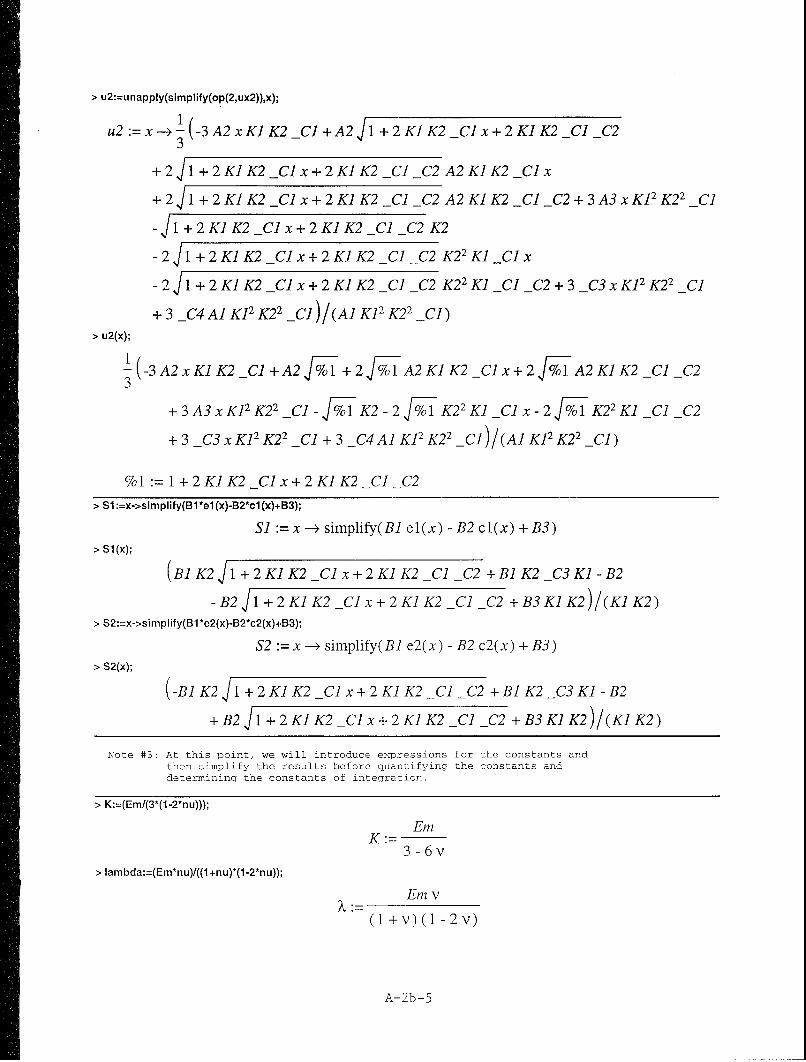
"> u2:=unapply(simplify(op(2,ux2)),x);
u2:=x- 4 31(-3A2xKIK2 CI +A2J I +2KI K2 _Clx+2KI K2 C1 _C23
+2j1 +2K1 K2 _Clx+2K1 K2 C _C2 A2K1K2 Clx
+2j1 +2K1 K2 _Clx+2K1 K2 Cl _C2 A2K1K2 Cl _C2+3A3xK12 K22 _C1
-J1 +2K1K2 _Clx+2K1K2 Cl _C2 K2
-2J1 +2K1K2 _Clx+2K1K2 Cl _C2 K22 K1 _Cl x
- 2 J 1 + 2 K1 K2 _C1 x + 2 K1 K2 _Cl _C2 K22 K1 _C1 _C2 + 3 _C3 x K12 K22 _C1
+ 3 _C4 A] K12 K22 _Cj )/(A] K12 K22 _Cl)"> u2(x);
I(-3A2xKIK2 Cl+A2 o1+2 J%1A2KIK2 _Clx+2 o1A2KIK2 Cl _C2
3+3A3xK12 K22 Cl- -%1K2-2 -%K2aK _Clx-2 %O1K22 K1 C1 _C2
+ 3 _C3 x K12 K22 _C1 + 3 _C4 Al K12 K22 _C1 )/(A1 K12 K22 _Cl)
%1 := 1 + 2 K1 K2 _Cl x + 2 K1 K2 _C] _C2
"> S$ :=x->simplify(Bl*el(x)-B2*cl(x)+B3);
Si x -> simplify(BJ el(x) - B2 cl(x) + B3)"> S1 (x);
(B1 K2 J 1 + 2 K1 K2 _Cl x + 2 K1 K2 _Cl _C2 + BI K2 _C3 KJ- B2
-B2 1 1 + 2 K1 K2 _Cl x + 2 K] K2 _Cl _C2 + B3 K1 K2)/(K] K2)"> S2:=x->simplify(B1 *e2(x)-B2*c2(x)+B3);
S2 := x - simplify(B] e2(x) - B2 c2(x) + B3)"> S2(x);
(-BI K2 J 1 + 2 K] K2 _Cl x + 2 K1K 2 _C] _C2 + BI K2 _C3 KJ - B2
+ B2 J 1 + 2 K1 K2 _C1 x + 2 K1 K2 _Cl _C2 + B3 KJ K2)/(Kl K2)
Note #3: At this point, we will introduce expressions for the constants andthen simplify the results before quantifying the constants anddetermining the constants of integration.
"> K:=(Em/(3*(1-2*nu)));
EmK:=
3 -6v"> lambda:=(Em*nu)/((1+nu)*(1-2*nu));
Em v
(1+ v)(1 -2v)
A-2b-5

"> mu:=Em/(2*(l+nu));
Em2+2v
"> alpha:=(rho*Vs)/(3*MWs);
1 p Vs
3 MWs
"> Ki :=(Vs*K)/(R*T);
Vs EmK1:=
(3-6v)RT"> K2:=3*alpha*(l +traps);
p Vs (I + traps)K2 :MWs
"> KI*K2;
Vs2 Em p ( 1 + traps)
(3 - 6 v) R T MWs"> A1 :=(]-2*nu);
A :=1 -2v
"> A2:=2*(l+nu)*alpha*(l+traps);
2 (1 +v)p Vs(l +traps)A2 :3 MWs
"> A3:=A2*cO;
2 (1 +v) p Vs (1 + traps)cOA3 :=- 3 MWs
> BI:=3*K;
EmB/ := 3 -3-6v
"> B2:=9*K*alpha*(l+traps);
Em p Vs ( 1 + traps)B2 :=3(3 - 6 v) MWs
"> B3:=B2*cO;
B3:=3 Em Vs (1 + traps) cO
(3 - 6 v) MWs
A-2b-6
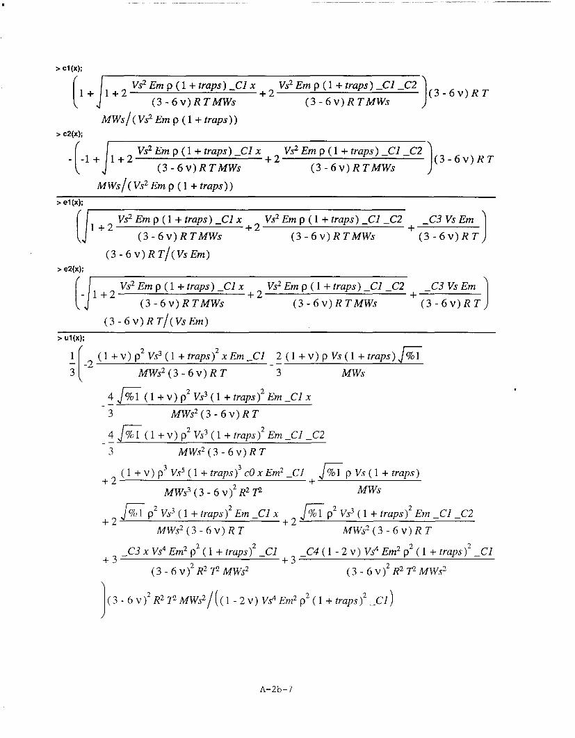
> cl (x);
+I Vs m Xp(+1traps) l x Vs2 m mp(1+traps) l C22(3 -(3-6v)RTMWs (3-6v)RTMWs
MWs/( Vs2 Em p (1 + traps))"> c2(x);
. /1+2 VsEm- p(1+traps)+Clx Vs2 Em p (1+traps)C C2 6v)-1+ 1+2 (3-6v)RTMWs (3-6v)RTMWs (3
MWs/(Vs2 Em p (1 + traps))
"> el (x);
1 Vs2 Emp(I +traps) Clx Vs2 Emp( +traps) C1 C2 C3 Vs Em11-2+2+
(3-6v)RTMWs (3-6v)RTMWs (3-6v)RTT
(3 - 6 v) R T/(Vs Em)"> e2(x); ! Vs2 Emp(1+traps)-Clx+2 Vs2 Emp(l+traps)-C _C2 C3VsEm
(3 - 6v) R TMWs (3 - 6v)R TMWs (3 - 6v) R T)
(3 - 6 v) R T/(Vs Em)
"> ul(x);
1r 2 (1+v)p2Vs3(1+traps)2xEm Cl 2(1+v)pVs(1+traps) %1MWs2 (3 - 6 v) R T 3 MWs
4 %1 (1+v)p2 Vs3 (1+ traps)2 Em Cx
3 MWs2 (3 - 6v)R T
4 %1 (1+v)p2 Vs3 (1 +traps)2 Em _Cl C2
3 MWs2 (3 - 6v) R T
+2 + v) P 3 Vs5 ( 1 + traps) 3 cO x Em2 Cl ol p Vs ( 1 +traps)
MWs3 (3 - 6 v)2 R2T2 MWs
%1 p 2 Vs 3 ( 1 + traps)2 Em C1 x %1 p 2 Vs3 (1 + traps)2 Em C1 C2+ 2 - +2 T
MWs 2 (3- 6 v) R T MWs 2 (3 - 6v) R T
+3 C3 X Vs4 Em 2 P2 (1 + traps)2 _C] C4 (1 - 2 v) Vs4 Em2 p 2 ( 1 + traps)2 _C1
(3-6 v) 2 R2 72 MWs2 (3-6 v) 2 R2 T2 MWs2
j(3-6v)2R2T2MWS2/((12v)VS4Em22 (1b+traps)2C1)
A-2b-7

Vs 2 Em p ( 1 + traps) _Cl x Vs 2 Em p ( 1 + traps) _Cl _C2%I := 1 +2- +2 -(3 - 6 v) R TMWs (3 - 6 v) R TMWs
A-2b-8

> u2(x);
1 ± (2+v)P2Vs3( 1 + traps)xEmCraps)3 MWs 2 (3 - 6 v) R T 3 MWs
4 %O1 ( 1 + V) p 2 Vs3 (1 + traps)2 Em _C1 x
3 MWs2 (3 - 6 v) R T
4 7%1 ( 1 + v) p2 Vs3 (1 + traps)2 Em C1 C2
3 MWs2 (3 - 6 v) R T+2 1 + V) p3 Vs5 ( 1 + traps) 3 cO x Em2 _C] - % Vs ( 1 + traps)
MWs3 (3-6 v) 2 R2 T2 MWs
2 V3( 2 2o%1 p Vs3 (1+ traps Em _CI x %1 p2 VS3 ( 1 + traps)2 Em C1 C2-2 -0/1_2
MWs (3 - 6 v) R T MWs2 (3 - 6 v) R T
+3 C3 X Vs4 Em2 p2 (1 + traps)2 _C] C4 (1 - 2 v) Vs4 Em2 p2 (1 + traps )2 _C]
(3-6 v)2 R2 T2 MWs2 (3-6 v)2 R2 T2 MWs2
(3-6 v) 2R 2 T2MWS2 /((1 -2v) VS4 EM2P2 (I +traps)2_C1 )
VS2 Em p (1 + traps) -C1 x Vs
2 Em p (1 + traps) -C1 C2%1:= 1 +2 +2
(3 - 6 v) R TMWs (3 - 6 v) R TMWs
"> S1 (x);
- (MWs _C3 Vs Em - 3 R TMWs + 6 R TMWs v + Em p Vs2 cO + Em p Vs2 cO traps)/(
(-1 + 2 v) Vs MWs)"> S2(x);
- (MWs _C3 Vs Em - 3 R TMWs + 6 R TMWs v + Em p Vs2 cO +Em p Vs2 cO traps)/(
(-1 + 2 v) Vs MWs)
"> Sl(x)-S2(x);
0
Note #4: The stresses are same for each solution root, and do not depend onthe position x! The stresses are therefore constant throughout thebody. We define a new stress function, Sx.
"> Sx:=S2(x);
Sx:: - (MWs _C3 Vs Em - 3 R TMWs + 6 R TMWs v +Em p Vs2 cO + Em p Vs2 cO traps)/(
(-1 +2v) VsMWs)
A-2b-9
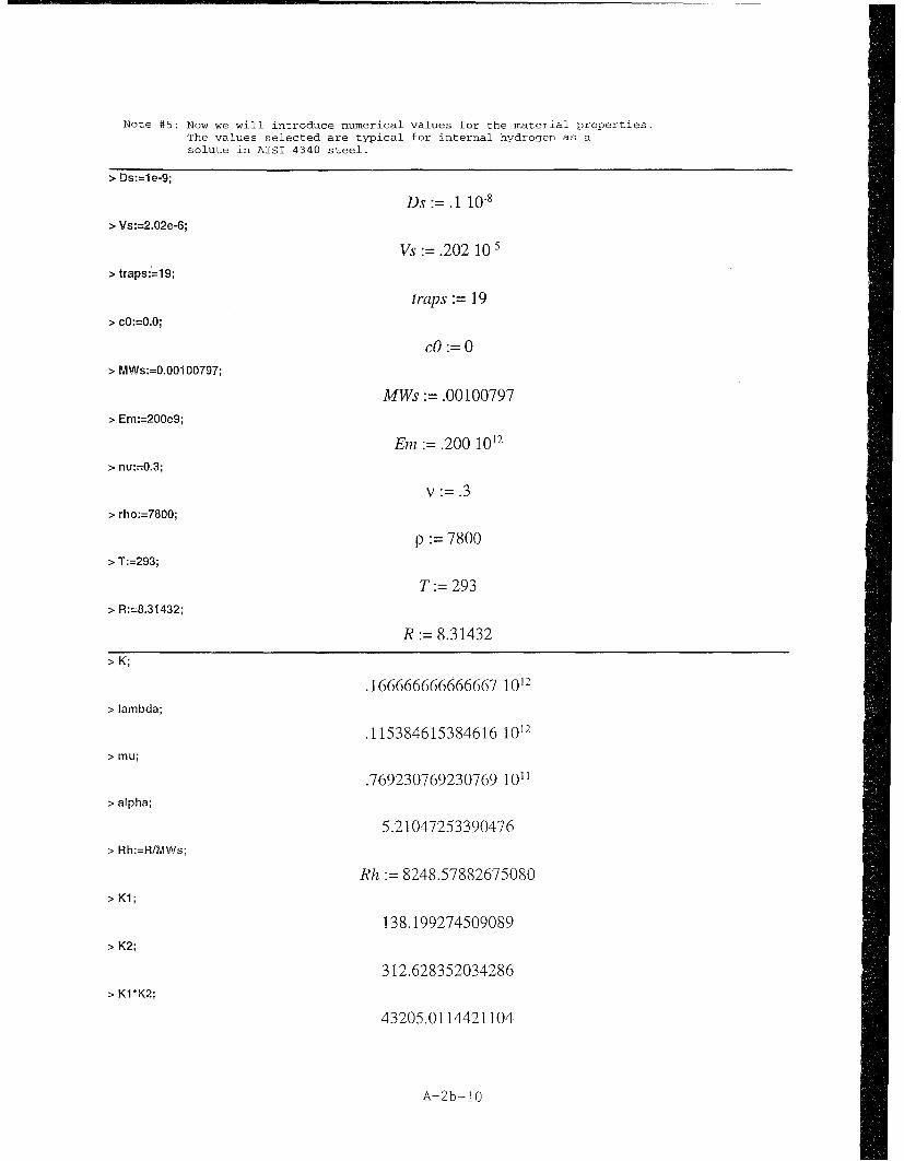
Note #5: Now we will introduce numerical values for the material properties.The values selected are typical for internal hydrogen as asolute in AISI 4340 steel.
"> Ds:=le-9;
Ds :=.1 10'"> Vs:=2.02e-6;
Vs :=.202 10.'"> traps:'=19;
traps := 19"> cO:=0.0;
cO:= 0
"> MWs:=0.00100797;
MWs :=.00100797"> Em:=200e9;
Em :=.200 1012
"> nu:=0.3;
v := .3"> rho:=7800;
p := 7800"> T:=293;
T:= 293"> R:=8.31432;
R:= 8.31432
> K;
,166666666666667 1012
"> lambda;
.115384615384616 1012
"> mu;
.769230769230769 1011"> alpha;
5.21047253390476"> Rh:=R/MWs;
Rh := 8248.57882675080"> K1;
138.199274509089"> K2;
312.628352034286"> KI*K2;
43205.0114421104
A-2b-1O0
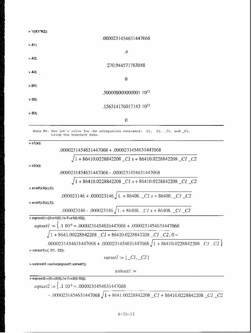
"> 1/(K1*K2);
.0000231454631447068"> Al;
.4"> A2;
270.944571763048"> A3;
0">B1;
.500000000000001 1012
"> B2;
.156314176017143 1015
"> B3;
0
Note #6: Now let's solve for the integration constants: _Cl, _C2, _C3, and _C4,using the boundary data.
"> cl(x);
.0000231454631447068 + .0000231454631447068
J 1 + 86410.0228842208 _C1 x + 86410.0228842208 _C1 _C2"> c2(x);
.0000231454631447068 - .0000231454631447068
, 1+ 86410.0228842208 _CI x + 86410.0228842208 _CI C2
"> evalf(cl(x),5);
.000023146 + .000023146 J 1. + 86408. _Cl x + 86408. _Cl _C2"> evalf(c2(x),5);
.000023146- .000023146 J 1. + 86408. _C1 x + 86408. _Cl _C2
"> eqnsetl:={O=cl (0),1 e-7=cl(0.10)};
eqnsetl := {. 1 10-6 = .0000231454631447068 + .0000231454631447068
J 1 + 8641.00228842208 _C1 + 86410.0228842208 Cl _C2,0 =
.0000231454631447068 + .0000231454631447068 J 1 + 86410.0228842208 _Cl _C2 }"> varsetl :={Cl ,_C2};
varset] _C], _C2"> solnsetl:=solve(eqnsetl,varsetl);
solnsetl
"> eqnset2:={O=c2(O),le-7=c2(0.10)};
eqnset2 := {. 1 10-6 = .0000231454631447068
- .0000231454631447068 J 1 + 8641.00228842208 _Cl + 86410.0228842208 _Cl _C2
A-2b-11

.0000231454631447068 - .0000231454631447068 J1 + 86410.0228842208 _Cl _C2 }"> varset2:={Cl ,_C2};
varset2 -C], _C2}"> solnset2:=solve(eqnset2,varset2);
solnset2 { C2 = 0, -C1 = -.997839749427893 10-6 }
"> asiign(soinset2);
Note #7: The solution cl(x) is not capable of satisfying the boundaryconditions, as evidenced by the lack of solution for the givenboundary conditions. The concentration function c2(x) is thecorrect solution in this case!
"> c2(x);
.0000231454631447068 - .0000231454631447068 J 1 - .0862233555828494 x"> pl :=plot(1 e6*c2(x/l OO),x=O..1 O,title='Concentration, c2(x) [ppm]'):"> P;
Concentration, c2(x) [ppm]0.1
0,08
0,08
0.04"
0.02'
0 2 8 10x
"> p2:=plot(1 e9*(c2(O)+((c2(0.10)-c2(0))10.1O)*x/100-c2(x/100)),x=O..10,title='Concentration Difference [ppb]'):"> p2;
Concentration Difference [ppb]
0.05
0.04
0.03
0.02:
2 4 G 8 10
x
A- 2b-12

> u2(x);
-.0156778440000000 x + .0186490538338527] 1 -_.0862233555828494x
- .00160798400000002 J 1 - .0862233555828494 x x + 2.49999999999999 _C3 x
+ .999999999999992 _C4
> eqnset3:={O=u2(0),O=u2(0.10)};
eqnset3 { 0 = .0186490538338527 + .999999999999992 _C4,
0 = .0 168405925050965 + .249999999999999 _C3 + .999999999999992 -C4 }> varset3:={_C3,_C4};
varset3 { _C3, -C4}> solnset3:=solve(eqnset3,varset3);
solnset3 { _C3 = .00723384531502524, _C4 = -.0186490538338529 }> assign(solnset3);> e2(x);
-.00723592799999998 J 1 - .0862233555828494 x + .00723384531502525
> p3:=plot(le6*e2(x/100),x=O..10,title='Dilatational Strain, e2(x) [ue]'):> p3;>
Dilatational Strain, e2(x) [uej
25
20
15
10
5
0 2 4 6 8 10
> u2(x);
.00240676928756317 x + .0186490538338527 Ji -_.0862233555828494 x
- .00160798400000002 jI -_.0862233555828494 xx - .0186490538338527
A-2b-13

"> p4:=plot(1 e6*u2(x/1 00),x=0..1 O,title='Displacement, u2(x) [urn]'):"> p4;
Displacemerqt, u2tx) [urn] 89 2 4 10
0
-0,02
-0.04
-0.06
-0.08
-0.1
-0.12
"> ex:=unapply(diff(u2(x),x),x);
1ex := x --> .00240676928756317 - .000803991999999991 1 - .0862233555828494 x
x+ .0000693228881017671 l-.0862233555828494x
- .00160798400000002 J 1 - .0862233555828494 x
"> p5:=plot(1 e6*ex(x/100),x=O..10,title='AxiaI Strain, ex(x) [ue]'):"> p5 ;
Axial Strain, ex(x) [ue]
4A-2-1
21 -
02 4 X 6810
-2!
A-2b-14 --

"> Sx;
-.104134248738053 107
"> J2(x);
-.997839749427893 10-15
"> evalf(u2(x),5);
.0024067 x + .018644 1.-.086222x-.0016072 .- .086222x x-.018650"> evalf(c2(x),5);
.000023146 -. 000023146j 1. -. 086222x"> evalf(e2(x),5);
-.0072359 11. - .086222 x + .0072338"> evalf(ex(x),5);
1 x.0024068 -. 00080399 + .000069323
.-. 086223x 1. -. 086223 x
- .0016080 J1. -. 086223 x
A-2b-15
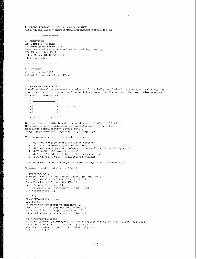
1. MAPLE PROGRAM DIRECTORY AND FILE NAME:/afs/nd.edu/user4/jthomas5/Maple/Transport/lDSSsol#2c.ms
2. ORIGINATOR:Dr. James P. ThomasUniversity of Notre DameDepartment of Aerospace and Mechanical Engineering374 Fitzpatrick HallNotre Dame, IN 46556-5637(219) 631-9371
3. HISTORY:Written: June-1994Latest Revision: 13-Feb-1995
4. PROGRAM DESCRIPTION:One-dimensional, steady-state analysis of the fully coupled solute transport and trappingequations using "plane stress" constitutive equations for stress. The particular problemsolved is shown below:
'I Ii l \ -- > x [m]/l I__ __ _ __ _
x=O x=0.010
Deformation variable boundary conditions: u(O)=O, u(0.10)=OConcentration variable boundary conditions: c(O)=O, c(0.10)=le-7Reference concentration level: cO=0.0Trapping parameter: traps=499 (high trapping)
The equations used in the analysis are:
1. dJ/dx=O (steady-state diffusion equation)2. J=Ds*(Kl*c*de/dx-dc/dx) (mass flux)3. dS/dx=0 (steady-state deformation equation with zero body forces)4. S=Bl*e-B2*c+B3 (axial stress)5. de/dx-K2*dc/dx=O (dilational strain gradient)6. e=Al*du/dx+A2*c-A3 (dilatational strain)
The constants used in the plane stress analysis are defined below:
Ds:=lattice diffusivity [m^2/sec]
Kl:=(Vs*K)/(R*T)Vs:= partial molar volume of solute [m^3/mol solute]K:= bulk modulus=Em/(3*(l-2*nu)) [N/m^2]Em:= Modulus of Elasticity [N/m^2]nu:= Poisson's ratio [1]R:= universal gas constant=8.31432 [J/mol-K]T:= temperature [K]
Bl:=3*KB2:=9*K*alpha*(l+traps)B3:=B2*cotraps:= Csr*Kr=trapping constant [1]Csr:= saturation trap concentration [1]Kr:= equilibrium trapping constant [1]cO:= reference solute concentration [1i
K2:=3*alpha*(l+traps)alpha:- (rho*Vs) / (3*MWs)=solute concentration expansion coefficient [m/m/Delc]rho:= mass density of the solid [kg/m^3]MWs:- molecular weight of the solute [kg/mol)Delc:= c-cO [1]
A-2c-i

Al: l=-2*nuA2:=2* (l+nu) *alpha* (l+traps)A3 : =A2*cO
5. REQUIRED INPUTS:
Ds:=lattice diffusivity [m^2/sec]Vs:= partial molar volume of solute [m^3/mol solute)traps:= Csr*Kr=trapping constant [1]cO:'= reference solute concentration [1]MWs:= molecular weight of the solute [kg/mol]
Em:= Modulus of Elasticity [Pa]nu:= Poisson's ratio [1]rho:= mass density of the solid [kg/m^3]
T:= temperature [K]
6. SYMBOLIC ANALYSIS:
"> Digits:=trunc(evalhf(Digits));
Digits:= 15
"> J:=Ds*(K1*K2*c(x)-l)*diff(c(x),x);
J:=Ds(KIK2c(x)- 1) c(x)
"> deqn:=diff(J,x)=O;
deqn:=DsK]K2 c(x) +Ds(K1K2c(x)- ) c(x) 0
"> csoln:=dsolve(deqn,c(x),explicit);
_C1 J1+2K]K2 _C1x+2K]K2 C] C2
csoln:: c(x) C- K] K2
I 1l 2K]K2 Clx+2K]K2 C1 C2~C4 2+JI2 K2
- _KC1 CK2
Note #1: There are apparently two "roots" to the solution for c(x) , Theboundary conditions will be used to select the proper one.
"> cl :=unapply(sirmplify(op(2,csoln[1 ])),x);
1 + J1 + 2 K] K2 _C] x + 2 K] K2 _C] _C2
K] K2"> cl (x);
1 +J1 + 2 K1 K2_C] x+ 2 K C K2_C] _C2
K1 K2
A-2c-2

"> c2:=unapply(simplify(op(2,csoln[2])),x);
c2: x -1 +j11 + 2K1K2 -C x + 2K1 K2 -CI C2
K] K2"> c2(x);
-1 +J1 + 2 K]K2 -CI x±+2 KK2 -CI C2
K] K2
"> Ji :=unapply(simplify(Ds*(K1 *K2*c1 (x)-1 )*diff(c1 (x),x),x));
> J1(x);
Ds CI"> J2:=unapply(simplify(Ds*(K1 *K2*c2(x)-1 )*diff(c2(x),x)));
J2:=( )Ds CI
" J2(x);
Ds C]
Note #2: The ebove results show that both mass flux solutions are identical
and equal to Ds*_Cl where -Cl is a constant of integration!
"> exi :=dsoIve(diff(e(x),x)-K2*diff (cl (x),x)=O,e(x));
ex] e~x IJ 1 2 K]K2 -C x + 2 K K2 -C1 C2 + C3 K1
"> el :=unapply(simplify(op(2,exl)),x);
el := x I + 2 K1K2 CI x + 2 KK2 -Cl C2 + -C3 KK]
"> el (x);
I 1+ 2 KK2 -C] x±+2 K]K2 -C] C2 + C3 K]
K]"> ex2:=dsolve(diff(e(x),x)-K2*diff(c2(x),x)=O,e(x));
ex2 ex) -j 1±+2 K]K2 CI x±+2 K]K2 -C] C2 + -C3 K
"> e2:=unapply(simplify(op(2,ex2)),x);
J ±2 K]K2 -CI x±+2 K K2 -C] C2 - -C3 Ke2 :=x --->_
K]"> e2(x);
JI+ ±2 K]K2 -C x + 2 K K2 -C] C2 - -C3 K
K]
A-2c--3
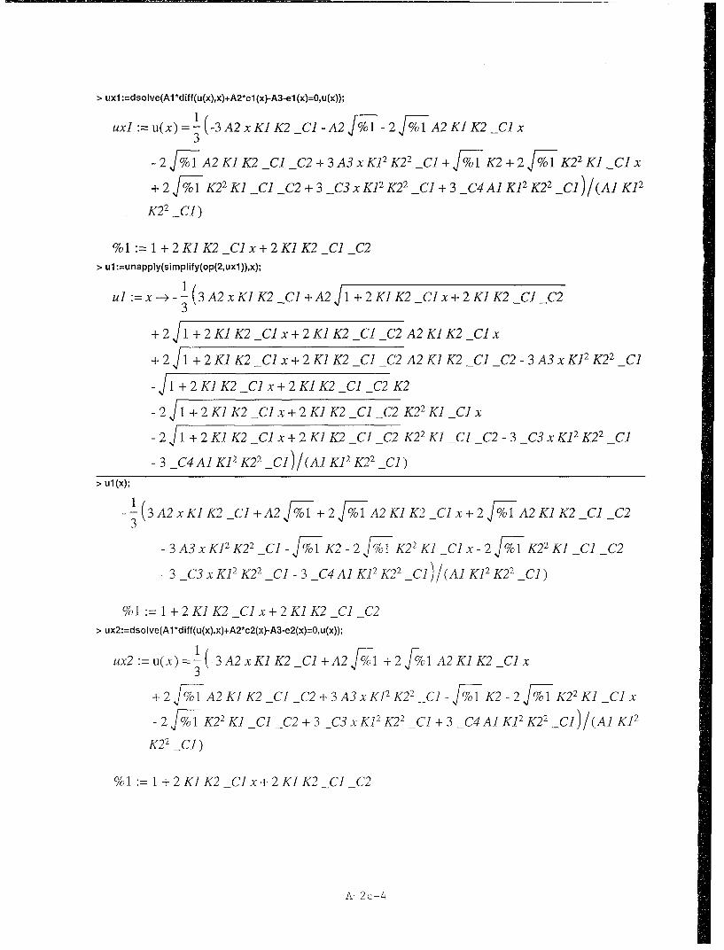
"> uxi :=dsolve(Al *diff (u~x),x)+A2*cl (x)-A3-el (x)=O,u(x));
uxl :==u(x)=-(-3 A2 x K1K2 _CJ -A2 %o,1 -2 %o,1 A2 K1K2 -Cl x3
-2%A2 KJK2 Cl _C2 +3 A3 XK12 K22 _CJ + 001 K2 +2 %1/ IK2 2 K Cl Flx-
+±2 %1o IK22 K1 Cl _C2 +3 _C3 xK12 K2 2 _Cl +3 _C4Al1K12 K2 2 -_Cl)/(Al K12
K22 CJ)
%1:= 1± 2 KK2 _Cl x±+2 K1K2 -Cl _C2"> ul:=unapply(simplify(op(2,uxl)),x);
ul:=x -~-- 1(3 A2 xKlK2 -Cl ±A2j1+2 K1K2 _Cl x±+2 K1K2 -Cl _C23
*2J1l+ 2 K1K2 _Cl x+ 2 K]K2 -Cl _C2 A2 KlK2 -Cl x
*+2Jt1+2 K]K2 _Cl x+ 2 K1K2 -Cl _C2 A2 K]K2 -Cl _C2-3 A3 XK12 K22 -Cl
-J + 2 K]K2 _Cl x±+2 K]K2 -Cl _C2 K2
- 2J1l+2 K]K2 _Cl x+ 2 K1K2 -Cl -C2K22 K] -Clx
-2J11±+2 K1K2 _Cl x+ 2 K1K2 -Cl _C2 K22 K1 -Cl -C2 -3 -C3 xKl2 K2 2 -Cl
-3 -C4A] K12 K22 _Cl)/(AlK12K22 _Cl)"> ul (X);
-(3 A2 x KK2 _C]±+A2 % I+ 2 %'o1 A2 KJK2 _Cl x +2 %1 A2 K]K2 -Cl _C23
-3A3xK12 K22 C- %1 K2 -2 %1 IK2 1 2 K1 _Cl x -2 %71 K22 K1 Cl _C2
- 3 _C3 x K]2 K22 _Cl -3 _C4 A] K]2 K22 -Cj )/(A] K12 K22 _Cl)
%1I:= I1+2 K]K2 _Cl x±+2 K]K2 _C] _C2"> ux2:=dsolve(A1 *diff(u(x),x)+A2*c2Cx)-A3-e2(x)=o~u(x));
ux2:=u(x)-(-3 A2 x KK2 _Cl±+A2 %1± +2 %1olA2 KlK2 Cl x3
+±2 5-1A2 KJK2 Cl _C2±+3 A3 xK12 K2 2 _C]- I1K2 -2 %1UK2 2 K1 Cl x
- 2 51-1K22 K1 -Cl _C2±+3 _C3 x K12 K2 2 _C]±+3 _C4 AJK]2 K22 _C)(A 1
K22 _C])
%1:= 1±2 K]K2 _Cl x± 2 KK2 -Cl _C2
A- 2 c-4

"> u2:=unapply(simplify(op(2,ux2)),x);
0:=x-4I ( -3A2xK1K2 C1+A2J1 +2K1K2 _Cx+2K1K2 Cl _C23
+2j1 +2K1 K2 _Clx+2KK2 Cl _C2 A2K1K2 Clx
+2j1 +2K1 K2 _Cx+2K1 K2 Cl _C2 A2K1K2 Cl _C2+3A3xK12 K2 2 _Cl
jI +2K1 K2 _Clx+2K1K2 Cl _C2 K2
-21 +2K1K2 _Clx+2K1K2 Cl _C2 K22 K1 _C1 x
- 2 J 1 + 2 K1 K2 _Cl x + 2 K1 K2 _Cl _C2 K22 K1 _C1 _C2 + 3 _C3 x K12 K22 _C1
+ 3 _C4 A] K12 K22 _C )/(Al K12 K22 _Cl)
"> u2(x);
I(-3A2xKIK2 C1+ A2 %o +2 %1A2K1K2 Cl x + 2 %o 1A2 KI K2 C1 _C2
3 .
+3A3xK12K22 Cl- %K22 % 2K _Clx-2F %1K22K1 Cl _C2S50 ,%1 K2- 2 %1 22K+ 3 _C3 x K12 K22 _-C]3 _C4AK 2K22 _cl )/(A1K12 K22 Cl)
%1:= 1 + 2 K1 K2 _CI x + 2 K1 K2 Cl _C2
"> Si :=x->simplify(Bl*el (x)-B2*cl (x)+B3);
Si:= x --- simplify(Bl el(x) - B2 cl(x) + B3)"> S1(x);
(BI K2 J1 + 2 KI K2 _Cl x + 2 K1 K2 _CI _C2 + B] K2 _C3 KJ - B2
-B2 J 1 + 2 K1 K2 _CI x + 2 K1 K2 _Cl _C2 + B3 KJ K2)/(K1 K2)"> S2:=x->simplify(Bl*e2(x)-B2*c2(x)+B3);
S2 := x --- simplify(Bl e2(x) - B2 c2(x) + B3)"> S2(x);
- (B1 K2 J I + 2 KJ K2 _Cl x + 2 K1 K2 _Cl _C2 - BJ K2 _C3 K] + B2
- B2 J 1 + 2 K1 K2 _CI x + 2 K1 K2 _Cl _C2- B3 K1 K2)/(Kl K2)
Note #3: At this point, we will introduce expressions for the constants andthen simplify the results before quantifying the constants anddetermining the constants of integration.
"> K:=(EmI(3*(1-2*nu)));
EinK:=
3-6v
"> lambda:=(Em*nu)/((1 +nu)*(1-2*nu));
Em V
(1 +v)(1 -2v)
A-2c-5

"> mu:=Ern(2*(l+nu));
Em
2+2v"> alpha:=(rho*Vs)/(3*MWs);
1 p Vs
3 MWs
"> Ki :=(Vs*K)/(R*T);
Vs EmK1.-
(3-6v)RT"> K2:=3*alpha*(1 +traps);
p Vs ( 1 + traps)K2 :MWs
"> KI*K2;
Vs2 Em p ( 1 + traps)
(3 - 6 v) R TMWs"> Al:=(1-2*nu);
A]:= 1 -2v"> A2:=2*(l+nu)*alpha*(l+traps);
2 (1 +v) p Vs(1 +traps)A2:=3 MWs
"> A3:=A2*cO;
2 (1 +v) p Vs (1 + traps) cOA3 :- 3 MWs
"> B1:=3*K;
EmBI :=3--3 -6v
"> B2:=9*K*alpha*(1 +traps);
Em p Vs (1 + traps)B2 =3(3 - 6 v) MWs
"> B3:=B2*cO;
B3:= 3 Em p Vs (1 + traps) cO
(3 - 6 v) MWs
A-2c-6

"> cl (x);
1+1+ 2 Vs 2 Emp(1traps)Clx +2 VS2 EMp (1 + traps)C1 C2 (3 -6v)RT1 1 (3-6v)RTMWs (3 -6v)RTMWs
MWs/(Vs2 Em p (1 + traps))
"> c2(x);
( Vs2 Emp(1+traps) -Cl2x Vs2 Emp(+traps)C1 -C2(1+2 (3-6v)RTMWs +2 (3-6v)RTMWs (3-6v)RT
MWs/(Vs2 Em p (1 + traps))
"> el(x);
I VS2 Em p (1 + traps) C1 x Vs2 Em p ( 1 + traps) -C1 C2 C3 Vs Em1+±2 - +2 - - +-(3 - 6 v) R TMWs (3 - 6 v) R TMWs (3 - 6 v) R T
(3 - 6 v) R T/(Vs Em)"> e2(x);
+ Vs2 Emp(l+traps1Clx Vs2 Emp(l+traps) _C1 C2 _CSVsEm
(3-6v)RTMWs (3-6v)RTMWs (3-6v)RT)
(3 - 6 v) R T/(Vs Em)
"> ul(x);
l1 (l+v)p2Vs3 (1+traps)2xEmC1 2(1+v)pVs(l+traps) %13 MWs2 (3 - 6 v) R T 3 MWs
4 [/ ( 1 + v) P2 Vs3 ( 1 + traps) 2 Em _C1 x
3 MWs2 (3 - 6v) R T
4 J% 1 (1 + v) P 2 Vs3 (1 + traps)2 Em _C1 C2
3 MWs2 (3 - 6 v) R T
2 +v)p 3 Vs5(I +traps)3 cOxEm2_C1 C] %c p Vs(1 +traps)
MWs3 (3 - 6 v)2 R2 MWs
2 2%12 p p Vs3 (1 + traps) Em C1 x 2%1 p 2 VS3 (1 + traps)2 Em C] C2-2- 2- -
MWs2 (3-6v)RT MWs2 (3 -6v)RT
C3 x Vs4 Em2 p2 (1 + traps)2 _C 3 C4 (I - 2 v) Vs4 Em2 p2 (1 + traps)2 _C]
(3 - 6 v) 2 R2 V MWs2 (3 - 6 v)2 R2 T2 MWs2
(3-6V)2R2 V MWs2/((1- 2v) Vs4 Em2 p2 (I+traps)2 C])
Vs2 Em p (1 + traps) _Cl x Vs2 Em p (1 + traps) C1 C2%1 :=1 +2 +2
(3 - 6 v) R TMWs (3 - 6v) R TMWs
A-2c-7

> u2(x);
+ 2 V(l+v)p2Vs3(l+traps)2xEm -C] 2(l+v)pVs(l+traps) F-%91
3 MWs2 (3 - 6 v) R T 3 MWs
4 % 1 (1 + v) p2 Vs3 (1 + traps)2 Em _C1 x3 MWs2 (3 - 6v) R T
%4 JO 1 ( 1 + v) p2 Vs3 (1 + traps)2 Em CJ C2
3 MWs2 (3 - 6v)R T
( +v)p 3 Vs5(1 +traps)3 cOxEm2 _Cl 0o p Vs(l +traps)+2 MWs3 (3 - 6 v)2 R22 X MWs
2% p Vs3 (1 + traps)2 EmCI x 2/-% p2 Vs3 ( 1 + traps)2 EmrC1 C2MWs2 (3- 6v) R T MWs2 (3 - 6v) R T
C3 x Vs 4 Em22p2 (1 + traps)2 _C] C4 (1 - 2 v) Vs4 Em2 p2 (1 + traps)2 _C1+3 -±3 2
(3 - 6 v)2 R2 T2 MWs2 (3-6 v)2 R2 T2 MWs2
(3 -6 v)2 R2 T2 MWs2/((1- 2v) Vs4 Em2 p2 ( 1 + traps)2 _C)
Vs2 Em p (1 + traps) -C1 x Vs2 Em p (1 + traps) -C1 C2%1: 1 +2 +2
(3 - 6 v) R TMWs (3 - 6v) R TMWs
"> S1 (x);
- (MWs _C3 Vs Em - 3 R TMWs + 6 R TMWs v + Em p Vs2 cO +Em p VS2 cO traps)/(
(-1 + 2 v) Vs MWs)
"> S2(x);
- (MWs _C3 Vs Em - 3 R TMWs + 6 R TMWs v +Em p Vs2 cO + Em p Vs2 cO traps)!(
(-1 +2v) VsMWs)"> S 1(x)-S2(x);
0
Note #4: The stresses are same for each solution root, and do not depend onthe position x! The stresses are therefore constant throughout thebody. We define a new stress function, Sx.
"> Sx:=S2(x);
Sx:= - (MWs _C3 Vs Em- 3 R T MWs + 6 R T MWs v +Em p Vs2 cO + Em p Vs2 cO traps)/(
(-1 +2v) VsMWs)
Note #5: Now we will introduce numerical values for the material properties.The values selected are typical for internal hydrogen as asolute in AISI 4340 steel.
A-2c-8

"> Ds:=le-9;
Ds:=.1 10-8"> Vs:=2.02e-6;
Vs :=.202 10i'"> traps:=499;
traps:= 499"> cO:=O.O;
cO:= 0"> MWs:=O.00100797;
MWs :=.00100797"> Em:=200e9;
Em :=.200 1012
"> nu:=0.3;
v :=.3"> rho:=7800;
p := 7800"> T:=293;
T:= 293"> R:=8.31432;
R:= 8.31432
> K;
.166666666666667 1012
"> lambda;
.115384615384616 1012
"> mu;
.769230769230769 1011"> alpha;
5.21047253390476"> Rh:=R/MWs;
Rh:= 8248.57882675080"> K1;
138.199274509089"> K2;
7815.70880085715"> KI*K2;
.108012528605276 107
"> 1/(K1*K2);
.925818525788271 10-6
A-2c-9

"> Al;
.4"> A2;
6773.61429407620"> A3;
0> B1;,
.500000000000001 1012
"> B2;
.390785440042860 1016
"> B3;
0
Note #6: Now let's solve for the integration constants: _CI, _C2, C3, and _C4,using the boundary data.
"> cl(x);
.925818525788271 10-6+ .925818525788271 10-6
J1 +_.216025057210552 107 _C1 x + .216025057210552 107 _C] _C2
"> c2(x);
.925818525788271 10-6 - .925818525788271 10-6
Ji +_.216025057210552 107 _C] x +.216025057210552 107 _C1 _C2
"> evalf(cl (x),5);
.92584 10-6+ .92584 10-6 1. + .21602 107 _C] x + .21602 107 _C] _C2
"> evalf(c2(x),5);
.92584 106- .92584 106 1. + .21602 107 C1 x + .21602 107 _C1 C2
"> eqnsetl :={0=c1 (0),1 e-7=cl (0.10)};
eqnset] := { 0 = .925818525788271 10-6
+ .925818525788271 10-6 ji +±.216025057210552 107 _C1 _C2,. 1 10-6
.925818525788271 10-6+ .925818525788271 10-6
Ji + 216025.057210552 _C] + .216025057210552 107 _C] _C2 }"> varsetl :={_Cl ,C2};
varset] -C2, CI }"> solnsetl :=solve(eqnsetl ,varsetl);
soInset]
"> eqnset2:={O=c2(0),le-7=c2(0.10)};
eqnset2 := {.1 10-6 .925818525788271 10-6 - .925818525788271 10-6
Ji + 216025.057210552 _C] + .216025057210552 107 _C] _C2, 0
A-2c-10

.925818525788271 10-6
-. 925818525788271 10-6 J1 + .216025057210552 107 C1 C2 }"> varset2:={C1 ,_C2};
varset2 -C2, -C1"> solnset2:=solve(eqnset2,varset2);
solnset2 { C2 = 0, _C1 = -.945993735697361 10-6 }"> assign(solnset2);
Note #7: The solution cl(x) is not capable of satisfying the boundaryconditions, as evidenced by the lack of solution for the givenboundary conditions. The concentration function c2(x) is thecorrect solution in this case!
"> c2(x);
.925818525788271 10-6 - .925818525788271 10-6 j1 - 2.04358350874846 x"> pl:=plot(le6*c2(x/1O0),x=O..1O,title='Concentration, c2(x) [ppm]'):
"> P1;
Concentration, c2(x) [ppm]0,1'
0.04
0.02
00 2 4 6 8 10x
"> p2:=plot(1 e9*(c2(0)+((c2(0.1 O)-c2(O))/O.1 0)*x/l 0O-c2(x/1 00)),x=O..1 O,title='Concentration Difference [ppb]'):"> p2;
Concentration Difference [ppb]1.4
1.2
1
0.8
0.41
0.2
002 4 G 8 10
S~A-2c-I11

"> u2(x);
-.0156778440000000 x + .000786845261334466 j1 - 2.04358350874846 x
- .00 160798399999998 J 1 - 2.04358350874846 x x + 2.49999999999998 _C3 x
+ .999999999999996 _C4"> eqnset3:={O=u2(0),O=u2(0.10)};
eqnset3 : 0 = .000786845261334466 + .999999999999996 _C4,
0 = -.00100935844318366 + .249999999999998 _C3 + .999999999999996 -C4 }"> varset3:=LC3,_C4};
varset3 := {-C3, -C4}"> solnset3:=solve(eqnset3,varset3);
solnset3 := { C4 = -.000786845261334466, _C3 = .00718481481807253 }"> assign(solnset3);
"> e2(x);
-.00723592799999998 J 1 - 2.04358350874846 x + .00718481481807253"> p3:=plot(le6*e2(x/100),x=0..10,title='Dilatational Strain, e2(x) [ue]'):"> p3;
Dilatational Strain, e2(x) [ue]
700500!
500
4001
300
200
100
0 2 4 6 8 10
> u2(x);
.00228419304518136 x + .000786845261334466 J1 - 2.04358350874846 x
- .00160798399999998 J 1 - 2.04358350874846 x x - .000786845261334466
A-2c-12

> p4:=plot(1 e6*u2(x/1 O0),x=O..1O,title='Displacement, u2(x) [urn]'):> p4;
Displacement, u2(x) [urn]02 4 X 6 8 10
0
-0.5
-1
-1.5'
-2
-2.5
-31
"> ex:=unapply(diff(u2(x),x),x);
1ex:= x -> .00228419304518136 - .000803991999999993 1J 1_-2.04358350874846x
x+ .00164302479236567 .j - 2.04358350874846
x
- .00160798399999998 j 1 - 2.04358350874846 x"> p5:=plot(1 e6*ex(x/100),x=0..10,title='Axial Strain, ex(x) [ue]'):"> p5;
Axial Strain, ex(x) [ue]
100
501
0) 2 4 "X 6 8 lo
-50
-100,
A-2c-13

"> Sx;
-.255565909637320 108
"> J2(x);
-.945993735697361 10-15
"> evalf(u2(x),5);
.0022826 x + .00078643j 1. - 2.0436 x - .0016069J 1. - 2.0436 x x - .00078689"> evalf(c2(x),5);
.92584 10-6 _ .92584 10-6 F1. - 2.0436 x"> evalf(e2(x),5);
-.0072359 1. - 2.0436 x + .0071848"> evalf(ex(x),5);
1 x.0022842-.00080399 +.0016430 - .0016080 l. -2.0436 x
S17- 2.0436 x 1.- 2.0436 x
A-2c-14

1. MAPLE PROGRAM DIRECTORY AND FILE NAME:/afs/nd.edu/user4/jthomas5/Maple/Transport/iDSSsol#2d.ms
2. ORIGINATOR:Dr. James P. ThomasUniversity of Notre DameDepartment of Aerospace and Mechanical Engineering374 Fitzpatrick HallNotre Dame, IN 46556-5637(219) 631-9371
3. HISTORY:Written: June-1994Latest Revision: 13-Feb-1995
4. PROGRAM DESCRIPTION:One-dimensional, steady-state analysis of the fully coupled solute transport and trappingequations using "plane stress" constitutive equations for stress. The particular problemsolved is shown below:
/I\ --- > x [m]
'I I
x=O x=0.010
Deformation variable boundary conditions: u(O)=O, u(0.10)=OConcentration variable boundary conditions: J(O)=O, c(0.10)=le-7Reference concentration level: cO=0.0Trapping parameter: traps=19 (low trapping)
The equations used in the analysis are:
1. dJ/dx=O (steady-state diffusion equation)2. J=Ds*(Kl*c*de/dx-dc/dx) (mass flux)3. dS/dx=O (steady-state deformation equation with zero body forces)4. S=Bl*e-B2*c+B3 (axial stress)5. de/dx-K2*dc/dx=O (dilational strain gradient)6. e=Al*du/dx+A2*c-A3 (dilatational strain)
The constants used in the plane stress analysis are defined below:
Ds:=lattice diffusivity [m^2/sec]
Kl:=(Vs*K)/(R*T)Vs:= partial molar volume of solute [m^3/mol solute]K:= bulk modulus=Em/(3*(l-2*nu)) [N/m^2]Em:= Modulus of Elasticity [N/m^2]nu:= Poisson's ratio [1)R:= universal gas constant=8.31432 [J/mol-K)T:= temperature [K)
Bi:=3*KB2:=9*K*alpha*(l+traps)B3:=B2*cotraps:= Csr*Kr=trapping constant [13Csr:= saturation trap concentration [1]Kr:= equilibrium trapping constant fl]cO:= reference solute concentration [1]
K2:=3*alpha*(l+traps)alpha:= (rho*Vs)/(3*MWs)=solute concentration expansion coefficient [m/m/Delc]rho:= mass density of the solid [kg/m^3]MWs:= molecular weight of the solute [kg/mol]Delc:= c-cO [L]
A- 2d-i

Al: l=-2*nuA2 :=2* (l+nu) *alpha* (l+traps)A3 : =A2 *cO
5. REQUIRED INPUTS:
Ds:=lattice diffusivity [m^2/sec]Vs:= partial molar volume of solute [m^3/mol solute]traps:= Csr*Kr=trapping constant [1]cO:= reference solute concentration [1]MWs:= molecular weight of the solute [kg/mol]
Em:= Modulus of Elasticity [Pa]nu:= Poisson's ratio [1]rho:= mass density of the solid [kg/m^3]
T:: temperature [K]
6. SYMBOLIC ANALYSIS:
"> Digits:=trunc(evalhf(Digits));
Digits:= 15
"> J:=Ds*(KI*K2*c(x)-I )*diff(c(x),x);
J:= Ds (K] K2 c(x) - 1) c(x)
"> deqn:=J=O;
deqn:= Ds (K1 K2 c(x) - 1) - (x) 0
"> csoln:=dsolve(deqn,c(x),explicit);
1csoln :=c(x) ,c(x) = _C1
K] K2
Note #1: There are apparently two "roots" to the solution for c(x). Thefirst solution is obviously incorrect in that the concentrationthroughout the rod is defined in terms of the constants Ki and K2.The second solution is adopted as correct.
"> c2:=unapply(simplify(op(2,csoln[2])),x);
c2 := x -4 _C1
"> c2(x);
_C]
"> J2:=unapply(simplify(Ds*(Kl*K2*c2(x)-I )*diff(c2(x),x)));
J2:= 0"> J2(x);
0
Note 42: The above result shows that the mass flux is identically zero, asit should be.
A-2d-2

Note #3: Since the concentration is constant, we have from the third governingequation that e(x) equals a constant.
"> e2:=x->_C2;
e2 := x -> _C2"> e2(x);
-C2
"> ux2:=dsolve(Al*diff(u(x),x)+A2*c2(x)-A3-e2(x)=O,u(x));
-x A2 _C1 + x A3 + x _C2 + _C3 Alux2 :=u(x) -A]
"> u2:=unapply(simplify(op(2,ux2)),x);
xA2 _C1 - xA3 - x _C2 - _C3 Alu2 := x --- -
A]
"> u2(x);
x A2 CI - x A3- x _C2 - _C3 Al
A]
"> S2:=x->simplify(Bl*e2(x)-B2*c2(x)+B3);
S2 x -> simplify(B] e2(x) - B2 c2(x) + B3)"> S2(x);
B] _C2 - B2 _C] + B3
Note #4: At this point, we will introduce expressions for the constants andthen simplify the results before quantifying the constants anddetermining the constants of integration.
"> K:=(Em/(3*(1-2*nu)));
EmK:=
3 -6v"> Iambda:=(Em*nu)I((1+nu)*(1-2*nu));
Em v
(1+ v) (1 -2v)"> mu:=Em/(2*(l+nu));
Em2+2v
"> alpha:=(rho*Vs)/(3*MWs);
1 p Vs
3 MWs"> K1 :=(Vs*K)I(R*T);
Vs EmK]
(3 -6v)RT
A-2d-3

"> K2:=3*alpha*(l+traps);
p Vs ( 1 + traps)K2 :MWs
"> KI*K2;
Vs 2 Em p (1 + traps)
(3 - 6 v) R TMWs"> A1 :=(1-2*nu);
A]:= 1 -2 v"> A2:=2*(l+nu)*alpha*(l +traps);
2 (1 +v) p Vs (1 + traps)A2:=3 MWs
"> A3:=A2*cO;
2 (1 +v) p Vs (1 + traps) cOA3.-3 MWs
"> B1:=3*K;
EmB1 := 3 -3 -6v
"> B2:=9*K*alpha*(l +traps);
B2 =3 Em p Vs (1 + traps)
(3 - 6 v) MWs"> B3:=B2*cO;
B3:= 3 Em p Vs ( 1 + traps) cO
(3 - 6 v) MWs
"> c2(x);
_C]
"> e2(x);
_C2
"> collect(u2(x),x);
(2(1 +±v) p Vs(1I +traps) C] 2 (1±+V) p Vs (1±+traps) cO _ C2 x3MWs 3 MWs + ) C
2 v+_C3
1 -2v
> S2(x);
Em(-_C2 MWs + p Vs _C] + p Vs _C] traps - p Vs cO - p Vs cO traps)
(-1 + 2 v) MWs
A-2d-4
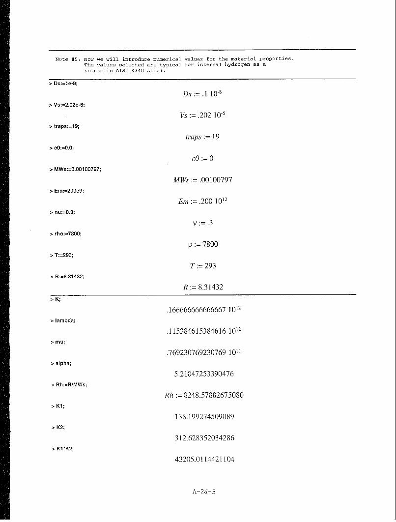
Note #5: Now we will introduce numerical values for the material properties.The values selected are typical for internal hydrogen as asolute in AISI 4340 steel.
"> Ds:=le-9;
Ds :=.1 10-1"> Vs:=2.02e-6;
Vs :=.202 10'"> traps:=19;
traps := 19"> cO:=0.0;
cO:= 0"> MWs:=0.00100797;
MWs :=.00100797"> Em:=200e9;
Em :=.200 1012
"> nu:=0.3;
v :=.3"> rho:=7800;
p := 7800"> T:=293;
T:= 293"> R:=8.31432;
R:= 8.31432
> K;
.166666666666667 1012
"> lambda;
.115384615384616 1012
"> mu;
.769230769230769 1011"> alpha;
5.21047253390476"> Rh:=RIMWs;
Rh := 8248.57882675080"> K1;
138.199274509089"> K2;
312.628352034286"> K1*K2;
43205.0114421104
A-2d-5

> 1/(Kl*KZ);
.0000231454631447068"> Al;
.4"> A2;
270.944571763048"> A3;
0"> B1;
.500000000000001 1012
"> B2;
.156314176017143 1015
"> B3;
0
Note #6: Now let's solve for the integration constants: _Cl, C2, _C3, and _C4,using the boundary data.
"> c2(x);
_C]"> _Cl :=1e-7;
CI :=. 1 10.6"> c2(x);
.1 10-6
"> u2(x);
-.0000677361429407620 x + 2.50000000000000 x _C2 + 1.00000000000000 _C3"> eqnsetl :={O.O~u2(O.O), 0.0=u2(0.10)};
eqnset] := { 0 = 1.00000000000000 _C3,
0 = -.677361429407620 10- + .250000000000000 _C2 + 1.00000000000000 _C3 I"> varsetl :=LC2,_C3};
varset] -C2, C3 }"> solnsetl :=solve(eqnsetl,varsetl);
solnset] := { C3 = 0, _C2 = .0000270944571763048 }"> assign(solnsetl);
A-2d-6

> c2(x);
.1 10-6
> e2(x);
.0000270944571763048> u2(x);
0> S2(x);
-.208418901356190 107
A-2d-7

1. MAPLE PROGRAM DIRECTORY AND FILE NAME:/afs/nd.edu/user4/jthomas5/Maple/Transport/lDSSsol#2e.ms
2. ORIGINATOR:Dr. James P. ThomasUniversity of Notre DameDepartment of Aerospace and Mechanical Engineering374 Fitzpatrick HallNotre Dame, IN 46556-5637(219) 631-9371
3. HISTORY:
Written: June-1994Latest Revision: 13-Feb-1995
4. PROGRAM DESCRIPTION:One-dimensional, steady-state analysis of the fully coupled solute transport and trappingequations using "plane stress" constitutive equations for stress. The particular problemsolved is shown below:
II I\ -- > x [m]'I I\'I I
x=O x=0.010
Deformation variable boundary conditions: u(O)=O, u(0.10)=OConcentration variable boundary conditions: J(O)=O, c(0.10)=le-7Reference concentration level: cO=0.0Trapping parameter: traps=499 (high trapping)
The equations used in the analysis are:
1. dJ/dx=O (steady-state diffusion equation)2. J=Ds*(Kl*c*de/dx-dc/dx) (mass flux)3. dS/dx=O (steady-state deformation equation with zero body forces)4. S=Bl*e-B2*c+B3 (axial stress)5. de/dx-K2*dc/dx=O (dilational strain gradient)6. e=Al*du/dx+A2*c-A3 (dilatational strain)
The constants used in the plane stress analysis are defined below:
Ds:=lattice diffusivity [m^2/sec]
Kl:=(Vs*K)/(R*T)Vs:= partial molar volume of solute [m^3/mol solute]K:= bulk modulus=Em/(3*(l-2*nu)) [N/m^2]Em:= Modulus of Elasticity [N/m^2]nu:- Poisson's ratio [1]R:- universal gas constant=8.31432 [J/mol-K]T:- temperature [K]
Bl:=3*KB2:=9*K*alpha*(l+traps)B3:-B2*cotraps:= Csr*Kr=trapping constant [1]Csr:= saturation trap concentration [1]Kr:= equilibrium trapping constant [1icO:= reference solute concentration [1]
K2:=3*aloha*(l+traps)alpha:= (rho*Vs) / (3*MWs)=solute concentration expansion coefficient [m/m/Delc]rho:= mass density of the solid [kg/m^3]MWs:= molecular weight of the solute [kg/mollDelc:= c-cO [1]
A-2e-1

Al: =l-2*nuA2:=2* (l+nu)*alpha* (l+traps)A3 : =A2*cO
5. REQUIRED INPUTS:
Ds:=lattice diffusivity [m^2/sec]Vs:= partial molar volume of solute [m^3/mol solute]traps:= Csr*Kr=trapping constant [1]cO:= reference solute concentration [1]MWs:z molecular weight of the solute [kg/mol]
Em:= Modulus of Elasticity [Pa]nu:= Poisson's ratio [1]rho:-- mass density of the solid [kg/m^3]
T:= temperature [K]
6. SYMBOLIC ANALYSIS:
"> Digits:=trunc(evalhf(Digits));
Digits:= 15
"> J:=Ds*(Kl*K2*c(x)-l)*diff(c(x),x);
J:=Ds(K]K2c(x)-l) C(X)
"> deqn:=J=O;
deqn:=Ds(K]K2c(x)-1) )-C(X) =0
"> csoln:=dsolve(deqn,c(x),explicit);
1csoln c(x) c(x) = -C]
K] K2
Note #1: There are apparently two "roots" to the solution for c(x) . Thefirst solution is obviously incorrect in that the concentrationthroughout the rod is defined in terms of the constants KI and K2.The second solution is adopted as correct.
"> c2:=unapply(simplify(op(2,csoln[2])),x);
c2 := x _C1"> c2(x);
_C]
"> J2:=unapply(simplify(Ds*(Kl*K2*c2(x)-I )*diff(c2(x),x)));
J2:= 0"> J2(x);
0
Note #2: The above result shows that the mass flux is identically zero, asit should be.
A-2e-2

Note #3: Since the concentration is constant, we have from the third governing
equation that e(x) equals a constant.
"> e2:=x->_C2;
e2 := x -- _C2"> e2(x);
_C2
"> ux2:=dsolve(Al*diff(u(x),x)+A2*c2(x)-A3-e2(x)=O,u(x));
-x A2 _C] + x A3 + x _C2 + _C3 A]ux2 :=u(x) =
A]
"> u2:=unapply(simplify(op(2,ux2)),x);
-xA2_CI +xA3+x C2+ _C3 A]u2 :x -4
Al"> u2(x);
-xA2 _C] +xA3+x C2 +_C3 A]
A]
"> S2:=x->simplify(Bl*e2(x)-B2*c2(x)+B3);
S2 := x -> simplify(B] e2(x) - B2 c2(x) + B3)
"> S2(x);
B] _C2 - B2 _CI + B3
Note #4: At this point, we will introduce expressions for the constants andthen simplify the results before quantifying the constants anddetermining the constants of integration.
"> K:=(Em/(3*(1-2*nu)));
EmK:=-
3 -6v"> lambda:=(Em*nu)/((1+nu)*(1-2*nu));
Em v
(l+v)(1 -2v)"> mu:=Em/(2*(1+nu));
Em2+2v
"> alpha:=(rho*Vs)/(3*MWs);
1 p VsOU.--
3 MWs"> Ki :=(Vs*K)/(R*T);
Vs EmK]
(3-6v)RT
A-2e-3
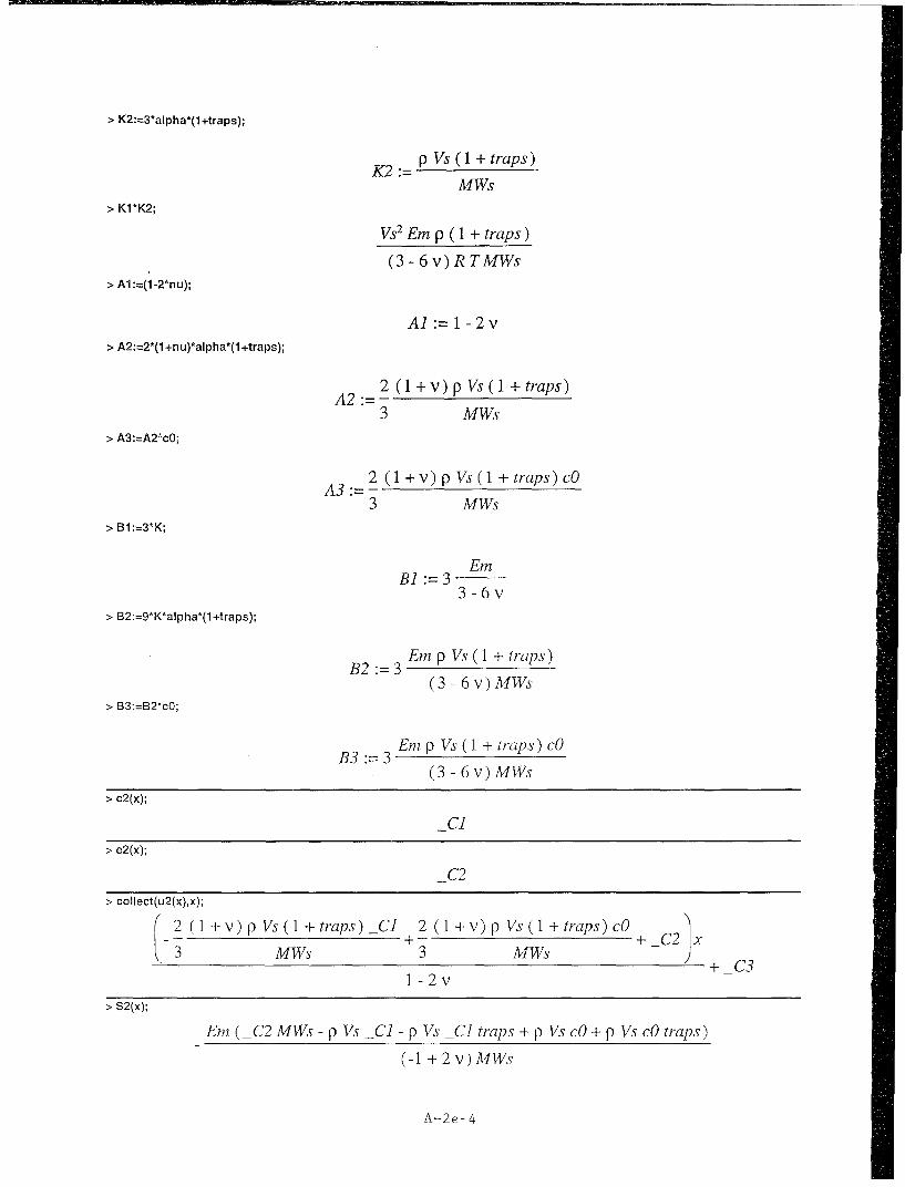
"> K2:=3*alpha*(l+traps);
K2 p Vs ( 1 + traps)MWs
"> Kl*K2;
Vs 2 Em p (1 + traps)
(3 - 6 v) R TMWs"> A1 :=(1-2*nu);
A] := 1 -2v
"> A2:=2*(l +nu)*alpha*(l +traps);
2 (1 +v)p Vs(1 +traps)A2:
3 MWs
"> A3:=A2*cO;
2 (l+v)pVs(l+traps)cOA3 :3 MWs
"> B1:=3*K;
EmB:= 3
3 -6v"> B2:=9*K*alpha*(l+traps);
132 :=3 Em p Vs (1 + traps)
(3 - 6 v) MWs"> B3:=B2*cO;
Em p Vs ( 1 + traps) cO
(3 - 6 v) MWs
"> c2(x);
C]
"> e2(x);
C2"> collect(u2(x),x);
2 (1 +v)p Vs(1+ traps) C1 2 (1 +v)p Vs(1 +traps) cO + -C2 x
3 MWs 3 MWs -+ _C3
1 -2v
"> S2(x);
Em (-C2 MWs - p Vs _C] - p Vs _C1 traps + p Vs cO + p Vs cO traps)
(-1 + 2v)MWs
A-2e-4

Note #5: Now we will introduce numerical values for the material properties.The values selected are typical for internal hydrogen as asolute in AISI 4340 steel.
"> Ds:=le-9;
Ds :.1 10-8"> Vs:=2.02e-6;
Vs :=.202 10-'"> traps:=499;
traps := 499"> cO:=0.0;
cO:= 0"> MWs:=O.00100797;
MWs :=.00100797"> Em:=200e9;
Em :=.200 1012
"> nu:=0.3;
V :=.3"> rho:=7800;
p := 7800"> T:=293;
T:= 293"> R:=8.31432;
R := 8.31432> K;
.166666666666667 1012
"> lambda;
.115384615384616 1012
"> mu;
.769230769230769 1011"> alpha;
5.21047253390476"> Rh:=R/MWs;
Rh := 8248.57882675080"> K1;
138.199274509089> K2;
7815.70880085715"> K1*K2;
.108012528605276 107
A-2e-5
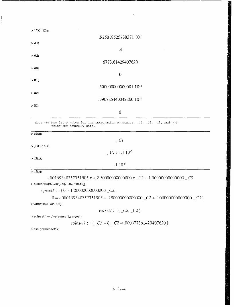
"> 1/(K1*K2);
.925818525788271 10-6
"> Al;
.4"> A2;
6773.61429407620"> A3;
0"> B1;
.500000000000001 1012
"> B2;
.390785440042860 1016
"> B3;
0
Note #6: Now let's solve for the integration constants: _Cl, C2, _C3, and C4,using the boundary data.
"> c2(x);
_CI"> C1:=le-7;
C1 := .1 10-6
"> c2(x);
.1 10-6
"> u2(x);
-.00169340357351905 x + 2.50000000000000 x _C2 + 1.00000000000000 _C3"> eqnsetl :={O.O=u2(0.0), 0.0=u2(0.10)};
eqnset] := {0 = 1.00000000000000 _C3,
0 =-.000169340357351905 + .250000000000000 _C2 + 1.00000000000000 _C3"> varsetl:=tC2,-C3};
varset] { C3, C2"> solnsetl :=solve(eqnsetl ,varsetl);
solnsetl { _C3 = 0, _C2 =.000677361429407620 }"> assign(solnsetl);
A-2e-6

"> c2(x);
.1 10-6"> e2(x);
.000677361429407620"> u2(x);
0"> S2(x);
-.521047253390490 108
A-2e-7

1. MAPLE PROGRAM DIRECTORY AND FILE NAME:/afs/nd.edu/user4/jthomas5/Maple/Transport/lDSSsol#3a.ms
2. ORIGINATOR:Dr. James P. ThomasUniversity of Notre DameDepartment of Aerospace and Mechanical Engineering374 Fitzpatrick HallNotre Dame, IN 46556-5637(219) 631-9371
3. HISTORY:Written: 12-Nov-1994Latest Revision: 13-Feb-1995
4. PROGRAM DESCRIPTION:One-dimensional, steady-state analysis of the fully coupled solute transport and trappingequations using "plane stress" constitutive equations for stress. The particular problem tobe solved is shown below. It is the 1-D SS transport problem, but with a (1/x)^(3/2)singular body force applied. This is meant to "simulate" the stress occurring at the tip ofa crack:
Body Force, Fx
Fx=A/x^(3/2)N(M/m^3]
---------------- > x[m]
'I-- > x[m]
x=O x=0.010
Deformation variable boundary conditions: u(O)=O, S(0.10)=QConcentration variable boundary conditions: J(O)=O, c(0.10)=le-7Reference concentration level: cO=0.0Trapping parameter: ltrap=19 (low trapping); htrap=499 (high trapping)Body Force: A=15xlO^6 [N/m^(3/2)]
The equations used in the analysis are:
1. dJ/dx=O (steady-state diffusion equation)2. J=Ds*(Kl*c*de/dx-dc/dx) (mass flux)3. dS/dx+Fx=0 (steady-state deformation equation with applied axial body force, Fx)4. S=Bl*e-B2*c+B3 (axial stress)5. de/dx-K2*dc/dx+Fx/Bl=O (dilational strain gradient)6. e=Al*du/dx+A2*c-A3 (dilatational strain)
The constants used in the plane stress analysis are defined below:
Ds:=lattice diffusivity [m^2/sec]
Kl:=(Vs*K)/(R*T)Vs:= partial molar volume of solute [m^3/mol solute]K:= bulk modulus=Em/(3*(l-2*nu)) [N/m^2)Em:= Modulus of Elasticity [N/m^2]nu:= Poisson's ratio [1lR:= universal gas constant=8.31432 [J/mol-K]T:= temperature [K]
A-3a-i

Bl:=3*KB2 : =9*K*alpha* (l+traps)B3 : =B2*co(1 or h)traps:= Csr*Kr=trapping constant [1]Csr:= saturation trap concentration [1]Kr:= equilibrium trapping constant [1]cO:= reference solute concentration [13
K2 : :3*alpha* (l+traps)alpha:= (rho*Vs)/(3*MWs)=solute concentration expansion coefficient [m/m/Delc]rho:= mass density of the solid [kg/m^3]MWs:= molecular weight of the solute [kg/mol]Delc:= c-cO [1]
Al: =l-2*nuA2 :2* (l+nu) *alpha* (l+traps)A3 :=A2*cO
5. REQUIRED INPUTS:
Ds:=lattice diffusivity [m^2/sec]Vs:= partial molar volume of solute [m^3/mol solute](1 and h)traps:= Csr*Kr=trapping constant [1]cO:= reference solute concentration [1]MWs:: molecular weight of the solute [kg/mol]
Em:= Modulus of Elasticity [Pa]nu:= Poisson's ratio [1]rho:= mass density of the solid [kg/m^31]
T:= temperature [K]
6. SYMBOLIC ANALYSIS:
"> restart;
"> Digits:=trunc(evalhf(Digits));
Digits:= 15
"> s:=x->Bl*e(x)-B2*c(x)+B3;
s := x --> B] e(x)- B2 c(x) + B3"> diff(s(x),x)+fx(x);
B1 e(x) -B2 c(x) + fx(x)
"> dedx:=x->K2*diff(c(x),x)-fx(x)/B1;
dedx:= x --> K2 diff(c(x), x) - fx(x)B1
"> j:=Ds*(Kl*c(x)*dedx(x)-diff(c(x),x));
j:= Ds Kc(x) K2 C(X) - (X) - c(x)
"> J := unapply(Ds*((K1K2*c(x)-l) diff(c(x),x)-(K1/B1) c(x)*F(x)),x);
K] c(x) F(x)J:= x --> Ds (K] K2 c(x) - 1) diff(c(x), x) - B]
"" J(X);
A-3a-2

Ds (K1 K2 c(x) - 1)a ( K c(x) - ~ x
"> F:=x->A/x^ (312);
AF:= x -> -x 312
Note #1: The governing differential equation in this case is J=constantbecause dJ/dx=O, and we are specifying the value of J(O)=0.Setting J(O)=constant produces a DE that is not easily solved.
"> deqnl :=collect(expand(J(x)I(Ds*K1 *K2)),diff(c(x),x))=0;
den =(CX 1 ) a'D') c(x)A =deqnl K2K2 BI X/22 0
"> solnI :=dsolve(deqnl,c(x));
ln(c(x)) Asolnl:=c(x)- +2 - A C1
K1K2 x K2 BI
Note #2: We will solve the above equation for c(x) and use this to define anew function with [x, A, K2, and _Cl) as the argument variables.
"> c:=(x,A,K2,C1 )->solve( c-(1/(KI*K2))*In(c)+(2*A)/(K2*B1 *xA(1/2)) = C0 ,c);/ ln( c)K]K A.
c:= (x, A, K2, C1) -> solve cL - -- + 2 A C1, cK]K2 K2 B] .x
"> c(x,A,K2,Cl);
W -K K 2 erK ] (2 x A-Cl K2 B ] x
KI K2
Note #3a: The above WO function is the "Lambert" function W( See theMaple help discussion of this function for further details.
Note #3b: The expression for the classical stress assisted diffusion (SAD)concentration is given by setting taking the limit of c(x) as K2->O.
"> csad:=(x,A,Cl)->Iimit(c(x,A,K2,Cl),K2=0);
csad:= (x, A, CI) --- lim c(x, A, K2, C])K2 -- 0
"> csad(x,A,C1);
(KJA~
"> dcdxl :=simplify(diff (c(x,A,K2,Cl),x));
KI(2: A -C] K2 BI x)~
dcdx] :- B
(I+ W -K1 K2 e ( xI x3/2 B] K2
A-3a-3

"> diff(W(f(x)),x);
(1 + W(f(x))) f(x)"> int(W(x),x);
XWx)W(x) x - ± W(x)
"> x:=(c,A,K2,Cl )->solve(c-(1/(K1 *K2))*In(c)+(2*A)/(K2*B1 *xA(1/2)) = C0 ,x);
x:= (c, A, K2, C]) --> solve c - n(c) 2 A C1, xK1 K2 K2 B] 'x
"> x(c,A,K2,Cl);
A2 K]2
4(c K] K2 BI - ln(c) BI - C] K] K2 B])
2
"> dxdc:=(c,A, K2,C1)->diff(x(c,A,K2,C1),c);
dxdc:= (c, A, K2, C]) --> diff(x(c, A, K2, C]), c)"> factor(dxdc(c,A,K2,C1));
SA2 K12 (cK K2- 1)83
B12 (-c K] K2 + ln(c) + C] K] K2)3 c"> factor(lldxdc(c,A,K2,Cl));
1 B1 2 (-c K] K2 + ln(c) + CJ K] K2)3 c
8 A 2 K12 (cK]K2 -1)
Note #4a: dx/dc->O as c->l/KI*K2, or conversely, dc/dx->infinity asc->I/KI*K2! This is apparently a critical point in themathematical solution for the concentration. The concentrationbecomes multivalued at this point.
Note #4b: We will now determine the value of the constant _Cl in terms ofthe concentration at the houndary c(01)=cl.
"> Cl ::solve(x(cI,A,K2,Cl)=0.1,Cl);
CI:= -.500000000000000
-2. B]2 ci K12 K22 + 2. B] 2 In(ci) K1 K2 + 12.6491106406735 B] K1 2 K2 A
B1 2 K12 K22
.500000000000000
-2. B1 2 cI K] 2 K22 + 2. B] 2 ln(ci) K] K2 - 12.6491106406735 B] K]2 K2 A
B] 2 K]2 K22
"> Cla:=(cl,A,K2)->expand(-.500000000000000/BIA2/K1 2/K22*(-2. *B1 A2*c*Kl K2*K2 A2+2.*Bl A2* n(cl)*Kl *K2+12.6491106406735*Bl *K1 ^2*K2*A));
CI a (cl, A, K2) -* expandj- 500000000000000
A-3a-4
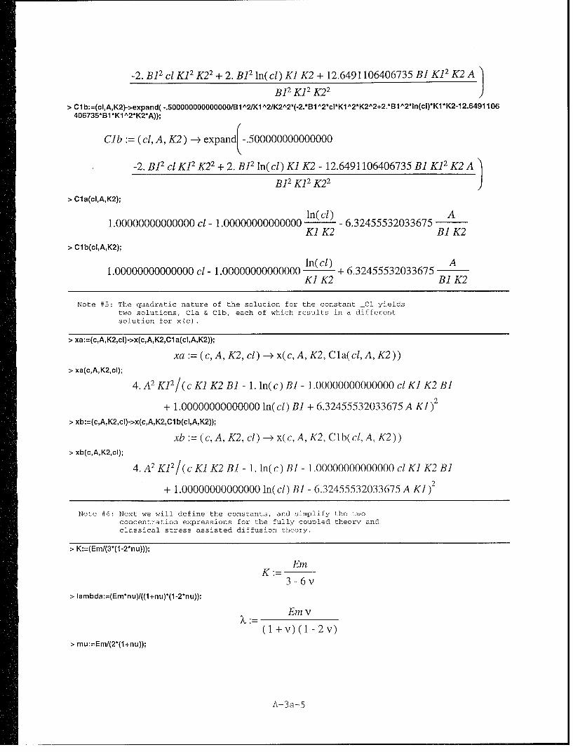
-2. B1 2 ci K12 K22 + 2. B12 ln(cl) K1 K2 + 12.6491106406735 BI K12 K2 A
B12 K12 K22
"> Cl b:=(cI,A,K2)->expand( -.5000000000000001B1 2/K1 A2/K2A2*(-2.*B1 A2*cI*K1 A2*K2A2+2.*B1 A2*In(cl)*K1 *K2-12.6491106406735*B1*K1 A2*K2*A));
Cib:= (cl, A, K2) --- expandr-.500000000000000-2. B12 Cl K12 K22 + 2. B1 2 ln(cl) K] K2 - 12.6491106406735 B] K12 K2 A
B12 K12 K22
"> Cla(cI,A,K2);
ln(cl) A1.00000000000000 ci - 1.00000000000000 - 6.32455532033675 A
K] K2 B] K2"> Clb(cI,A,K2);
ln(ci) A1.00000000000000 ci - 1.00000000000000 -- + 6.32455532033675 A
K1 K2 BI K2
Note #5: The quadratic nature of the solution for the constant _Cl yieldstwo solutions, Cla & Clb, each of which results in a differentsolution for x(c).
"> xa:=(c,A,K2,cl)->x(c,A,K2,Cla(cI,A,K2));
xa:= (c, A, K2, cl) -- >x(c, A, K2, Cla(cl, A, K2))"> xa(c,A,K2,cI);
4. A2 K12/(C K] K2 B] - 1. In(c) B] - 1.00000000000000 ci K] K2 B]
+ 1.00000000000000 ln(cl) B] + 6.32455532033675 A K] 2
"> xb:=(c,A,K2,cl)->x(c,A,K2,Clb(cI,A,K2));
xb:= (c, A, K2, cl) --> x(c, A, K2, Clb(cl, A, K2))"> xb(c,A,K2,cI);
4. A2 K]2 /(c KI K2 B] - 1. ln(c) B] - 1.00000000000000 cl K] K2 B]
+ 1.00000000000000 ln(cl) B] - 6.32455532033675 A K] 2
Note #6: Next we will define the constants, and simplify the twoconcentration expressions for the fully coupled theory andclassical stress assisted diffusion theory.
5 > K::(Em/(3*(1-2*nu)));
EEmK:=
3 -6v"> lambda:=(Em*nu)/((l+nu)*(1-2*nu));
Em v
(1+ v)(l -2v)"> mu::Em/(2*(1A+nu));
A-3a-5

Em
2 +2 v"> alpha:=(rho*Vs)I(3*MWs);
1 p Vs
3 MWs"> Ki :=(Vs*K)I(R*T);
Vs EmK]
(3 - 6v)R T"> K2:=3*alpha*(l +traps);
K2=p Vs (I + traps)
MWs
A] 1= -2 v"> A2:=2*(l +nu)*alpha*(1±+traps);
A2=2 (1±+v)p Vs(1±+traps)3 MWs
"> A3:=A2*cO;
A3 2 (1 + V) p Vs (1 + traps) cO
3 MWs"> B1:=3*K;
Em3-6v3
"> B2:=9*K~alpha*(1 +traps);
B2=3Em p Vs (1 I± traps)
(3 - 6 v) MWs"> B3:=B2*cO;
B3=3Em p Vs (1 + traps) cO
(3 - 6 v) MWs"> Ds-=le-9;
Ds:z=.1 10-'"> Vs:=2.02e-6;
Vs:=.202 10-1"> Itraps:=1 9;
itraps 19"> htraps:=499;
htraps 499
A-3a-6
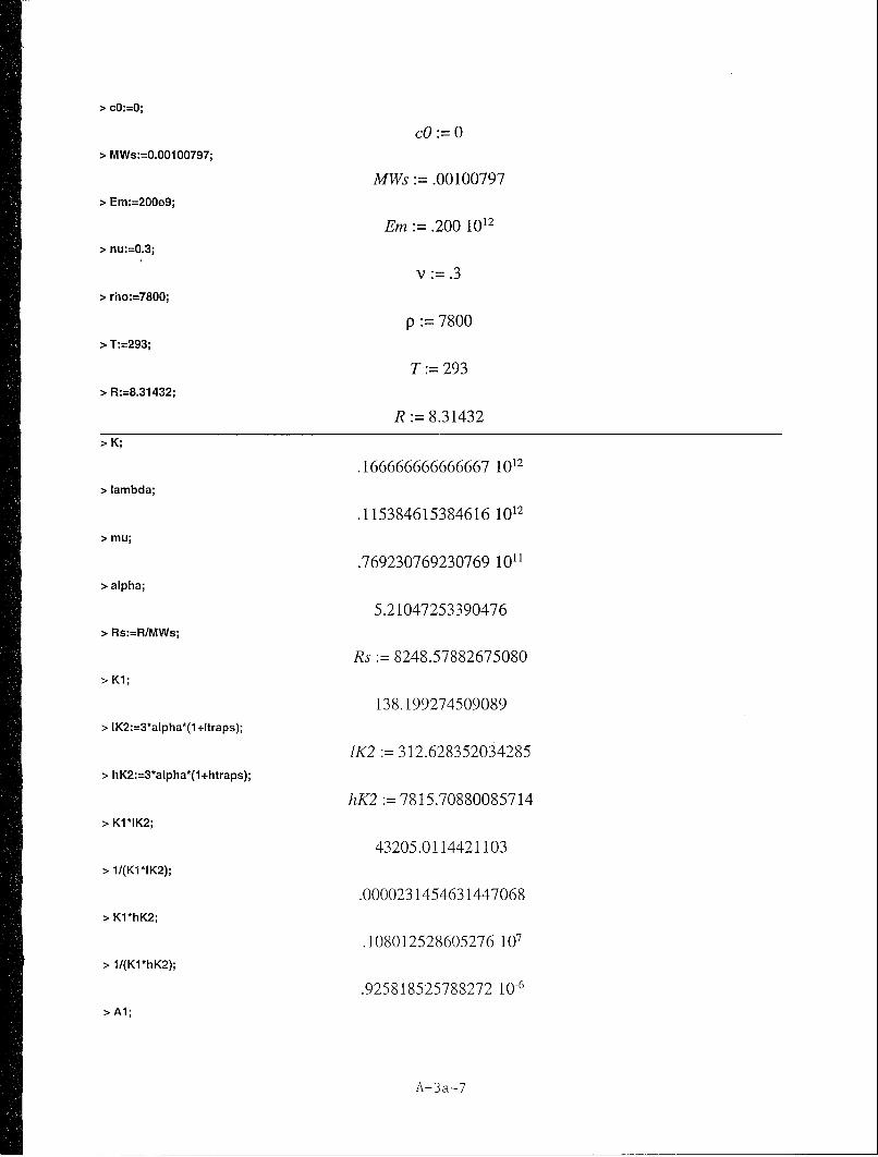
"> cO:=0;
cO:= 0"> MWs:=0.00100797;
MWs :=.00100797"> Em:=200e9;
Em :=.200 1012
"> nu:=0.3;
v :=.3"> rho:=7800;
p := 7800"> T:=293;
T:= 293"> R:=8.31432;
R:= 8.31432
> K;
.166666666666667 1012
"> lambda;
.115384615384616 1012
"> mu;
.769230769230769 1011"> alpha;
5.21047253390476"> Rs:=R/MWs;
Rs:= 8248.57882675080"> K1;
138.199274509089"> IK2:=3*alpha*(1 +ltraps);
lK2 312.628352034285"> hK2:=3*alpha*(l+htraps);
hK2 7815.70880085714"> KI*IK2;
43205.0114421103"> 1/(Kl *IK2);
.0000231454631447068"> Kl*hK2;
.108012528605276 107
"> 1I(K1*hK2);
.925818525788272 10-6
"> Al;
A-3a-7
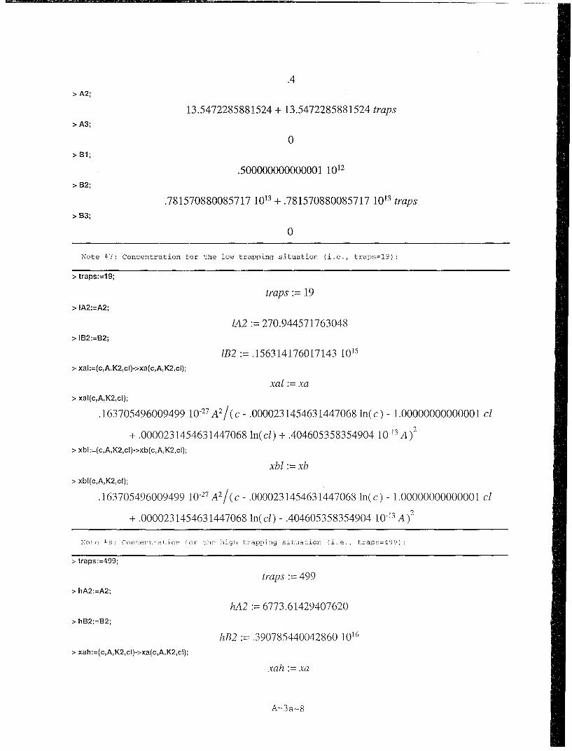
.4"> A2;
13.5472285881524 + 13.5472285881524 traps"> A3;
0"> B1;
.500000000000001 1012
"> B2;
.781570880085717 1013 + .781570880085717 1013 traps"> B3;
0
Note #7: Concentration for the low trapping situation (i.e., traps=19):
"> traps:=19;
traps := 19"> IA2:=A2;
IA2 := 270.944571763048"> IB2:=B2;
1B2 := .156314176017143 1015"> xal:=(c,A,K2,cl)->xa(c,A,K2,cI);
xal := xa"> xal(c,A,K2,cI);
.163705496009499 10-27 A2/( c - .0000231454631447068 ln(c) - 1.00000000000001 cl
+ .0000231454631447068 ln(cl) + .404605358354904 10-13 A)2
"> xbl:=(c,A,K2,cl)->xb(c,A,K2,cl);
xbl := xb"> xbl(c,A,K2,cI);
.163705496009499 10-27 A2/( c - .0000231454631447068 ln( c) - 1.00000000000001 cl
+ .0000231454631447068 ln(cl) - .404605358354904 10-13 A )2
Note #8: Concentration for the high trapping situation (i.e., traps=499):
"> traps:=499;
traps := 499"> hA2:=A2;
hA2 := 6773.61429407620"> hB2:=B2;
hB2 := .390785440042860 1016
"> xah:=(c,A,K2,cl)->xa(c,A,K2,cl);
xah := xa
A-3a-8

"> xah(c,A,K2,cI);
.261928793615197 1o303oA2/(c -.925818525788271 10-6 ln(c) - 1.00000000000001 ci
+ .925818525788275 10-6 ln(cl) + .161842143341962 10.14 A) 2
"> xbh:=(c,A,K2,cI)->xb(c,A,K2,cl);
xbh := xb"> xbh(c,A,K2,cl);
.261928793615 197 10-30A2/(c - .925818525788271 10-6 ln(c) - 1.00000000000001 ci
+ .925818525788275 10-6 ln(cl) - .161842143341962 10-1' A) 2
Note #9: Concentration for SAD:
"> csad(x,A,cI)->-1 .*ln(cI)+.551 68OO588e-9*AIXA(1I12);
csad(x, A, ci) -ý -1. ln(cl) + .5516800588 10-1
"> Csadl(x,A,cI);
CsadlI(x, A, ci)
"> with(plots);
[animate, animate3d, conformal, contourplot, cylinderplot, densilyplot, display, display3d,
fie ldplot, fieldplo t3d, gradp lot, gradplot3d, implicitplot, implicitplot3d, loglogplot,
logplot, matrixplot, odeplot, pointplot, polarplot, polygonpiot, polygonplot3d,
polyhedraplot, replot, setoptions, setoptions3d, spacecurve, sparsematrixplot,
sphereplot, surfdata, textplot, textplot3d, tubeplot]
"> logplot({xal(c,15e6,1K2,1e-7),"> xbl(c,15e6,1K2,le-7fl,c=le-7..1.5e-7,"> title='xa (upper) & xb (lower) -vs- c (Low Trapping), c(L)=le-7');
xa (upper) & xb (lower) -vs.- c (Low Trapping), c(L)=1 e-7
le-07 1.1e-07 1.2e-07 1.3e-07 1.4e-07 1.5e-07C
"> Iogplot({xah(c,15e6,hK2,Ie-7),"> xbh(c,15e6,hK2,le-7)},c=le-7..1.5e-7,
A- 3a- 9

> title='xa (upper) & xb (lower) -vs- c (High Trapping), c(L)=le-7');
xa (upper) &xb (lower) -vs-c (High Trapping), c(L)=le-7
10,I
1,!
Ie-07 i1le-07 1,2e-07 1.3e-07 1,4e-07 1,5e-07C
Note #11: The above plots show that the Clb parameter is clearly correctfor c(L)=le-7. The xa(c) solution predicts a singularityat the minimum concentration level on the rod, which is of nophysical use. We must now determine, however, whether the xb(c)solution is valid for all c if c(L)=le-7.
"> logplot(xbl(c,15e6,1K2,1e-7),"> c=le-7..2e-4,title='xb -vs- c (Low Trapping), c(L)=l e-7');
xb -vs-c (Low Trapping), c(L)=le-7
0.1
0,01
0.001
0.0001
le-05
2e-05 4e-05 Se-05 8e-05 0,00010.00012).000140,[email protected]
"> logplot(xbh(c,15e6,hK2,1 e-7),"> c=le-7..1e-5,title='xb -vs- c (High Trapping), c(L)=le-7');
A-3a-10
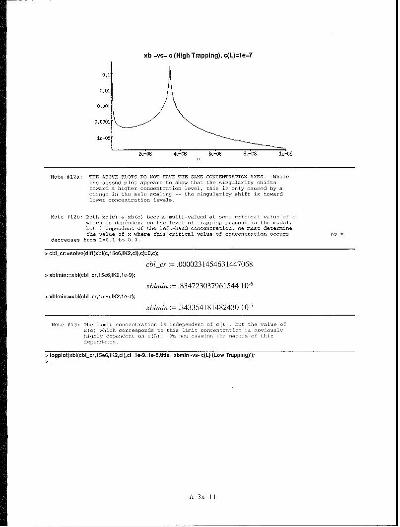
xb -vs-c (High Trapping), c(L)=le-7
0.1
0.01
0.001
0.0001
le-05
2e-06 4e-06 6e-06 8e-06 le-05C
Note #12a: THE ABOVE PLOTS DO NOT HAVE THE SAME CONCENTRATION AXES. Whilethe second plot appears to show that the singularity shiftstoward a higher concentration level, this is only caused by achange in the axis scaling -- the singularity shift is towardlower concentration levels.
Note #12b: Both xa(c) & xb(c) become multi-valued at some critical value of cwhich is dependent on the level of trapping present in the model,but independent of the left-hand concentration. We must determinethe value of x where this critical value of concentration occurs as x
decreases from L=0.1 to 0.0.
"> cblcr:=solve(diff(xbl(c,15e6,1K2,cl),c)=O,c);
cblcr:= .0000231454631447068"> xblmin:=xbl(cblcr,1 5e6,1K2,1 e-9);
xblmin :=.834723037961544 10-6
"> xblmin:=xbl(cbl-cr,15e6,1K2,le-7);
xblmin:=.343354181482430 10-5
Note #13: The limit concentration is independent of c(L), but the value ofx(c) which corresponds to this limit concentration is obviouslyhighly dependent on c(L). We now examine the nature of thisdependence.
"> Iogplot(xbl(cbl-cr,15e6,1K2,cl),cl=le-9..le-5,title='xbmin -vs- c(L) (Low Trapping)');
A-3a-1 1

xbmnin -vs- c(L) (Low Trapping)
0,0001
0 2.001e-06 4.001e-06 C16.001e-06 8.0ole-06
"> cbh-cr:=soIve(diff (xbh(c,l 5e6,hK2,cI),c)=O,c);
cbh~cr:=.925818525788272 10-6"> xbhmin:=xbh(cbh_cr,15e6,hK2,le-9);
xbhmin:=.200363349240182 10-'"> xbhmin:=xbh(cbh-cr,1 5e6,hK2,l e-7);
xbhmin:=.0000371878414183777"> Iogplot(xbh(cbh-cr,1 5e6,hK2,cI),cI=1 e-9..1 e-5,title='xbmin -vs- c(L) (High Trapping)');
xbmnin -vs- c(L) (High Trapping)
le-05
le-QE -0 2.O0le-06 4,O0le-08 6,O0le-06 8.001e-06
Note #14: The threshold level of c(L) at which xb(c) is no longer valid andxa(c) hecomnes the physicelly meaningful solution may also he
determined.
"> solve(diff(xbh(cbh-cr,15e6,hK2,cI),cl)=0,cI);
.925818525788271 10-6
"> logplot(xbh(c,15e6,hK2,le-6),c=le-6..1.5e-6,title='xb -vs- c (High Trapping) c(L)=1e-6');
A-3a-12
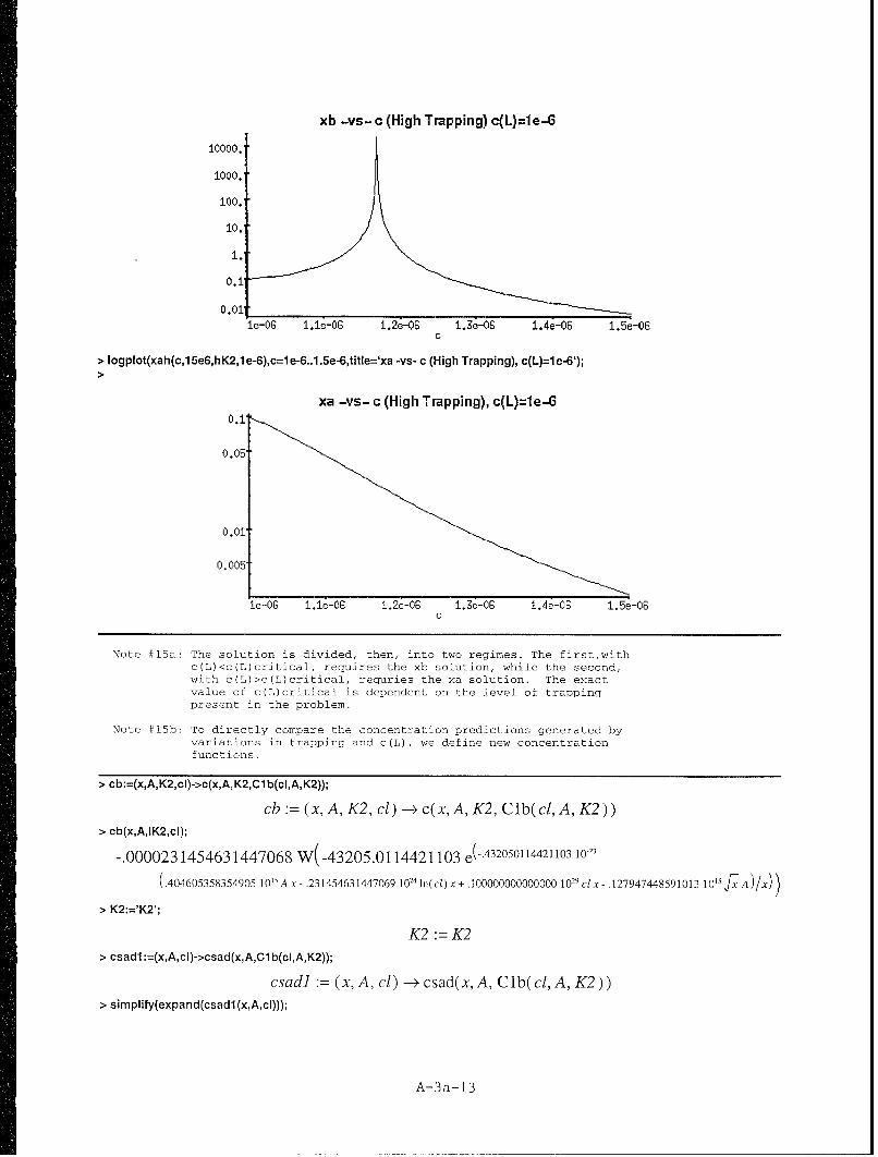
xb -vs-c (High Trapping) c(L)=le-6
10000.
1000.
100.
10.
0.1
0.01tle-06 1.le-06 1.2e-06 1.3e-06 1.4e-06 1.5e-06
C
> Iogplot(xah(c,15e6,hK2,1 e-6),c=1 e-6..1.5e-6,title='xa -vs- c (High Trapping), c(L)=1e-6');
xa -vs-c (High Trapping), c(L)=le-60.1" .
0.05'
0.01'
le-06 1.1e-06 1.2e-06 1.3e-06 1.4e-06 1.5e-06c
Note #15a: The solution is divided, then, into two regimes. The first,withc(L)<c(L)critical, requires the xb solution, while the second,with c(L)>c(L)critical, requries the xa solution. The exactvalue of c(L)critical is dependent on the level of trappingpresent in the problem.
Note #15b: To directly compare the concentration predictions generated byvariations in trapping and c(L), we define new concentrationfunctions.
"> cb:=(x,A,K2,cl)->c(x,A,K2,Clb(cI,A,K2));
cb := (x, A, K2, cI) -> c(x, A, K2, Clb(cl, A, K2))"> cb(x,AIK2,cl);
-.0000231454631447068 W(-43205.0114421103 e(-432050114421103 10.23
(.404605358354905 1015 A x - .231454631447069 10' ln(cl) x+.100000000000000 1029 cl X- .127947448591013 10"5.7 A)/x))
"> K2:='K2';
K2 := K2"> csadl :=(x,A,cl)->csad(x,A,Clb(cI,A,K2));
csad] := (x, A, cl) --> csad(x, A, Clb(cl, A, K2))"> simplify(expand(csadl(x,A,cl)));
A-3a-13

12500000000000129817044607271 ~-221118839214542 10.21 A.959102 03J 20000001"
cl A2(5.79056941504210100 J 2 0
"> p4:=Iogplot(cb(x,l 5e6,1 K2,1 e-7),x=l e-6..1 e-4,title='FC:cb(x) -vs- x (Low Trapping) c(L)=l e-7'):"> p 4 ;
FC:cb(x) -vs- x (Low Trapping) c(L)=le-7
le-OS
5e-0C
le-O6
5e-07'
2e-05 4e-05 Ge-05 8e-05 0.0001x
"> p5:=logplot(cb(x,1 5e6,hK2,1 e-7),x=l e-6..1 e-4,resolution=1 00000,"> title='FC:cb(x) -vs- x (High Trapping) c(L)=le-7'):"> p5;
FC:cb(x) -vs-x (High Trapping) c(L)=le-7
8e-07'
Se-07'
5e-07'
4e-07'
3e-07' - -- _ _
2e-05 4e-05 Se-05 8e-05 0.0001x
"> p6:=logplot(esadl (x,1 5e6,1 e-7),x=l e-6..1 e-4,"> resolution=10000,title='SAD:c(x) -vs- x'):"> p6;
A-3a-14

SAD :c(x) -vs- x
0.0001
le-05
ie-06
2e-05 4e-05 6e-05 Be-05 0.0001x
> display([p4,p5,p6],title='(c(L)=le-7):cb (L.T.), cb (H.T.), csadl -vs- x');
(c(L)=l e-7):cb (L.T.), cb (H.T.), csadl -vs- x
0.00015e-05
le-Og"5e-06"
le-OG5e-07
2e-05 4e-05 Ge-05 Be-05 0.0001x
Note #16: The above plots indicate that the difference between SAD andFully Coupled hydrogen concentration is strongly dependent onthe degree of trapping.
"> logplot(cb(x,l 5e6,hK2,1 e-7)-csadl (x,1 5e6,1 e-7),x=l e-6..1 e-4,"> resolution=10000,title='[FC:cb (H.T.)-SAD:c(x)] -vs- x (close-up)');
[FC:cb (H.T.)-SAD:c(x)] -vs- x (close-up)5e-07
2e-07
le-07
5e-081___________________________________
2e-05 4e-05 x Ge-05 8e-05 0.0001
"> Iogplot(cb(x,1 5e6,hK2,1 e-7)-csadl (x,1 5e6,1 e-7),x=l e-6..1 e-1,"> resolution=10000,title='[FC:cb (H.T.)-SAD:c(xfl -vs- x (full-length)');
A-3a--15

[FC:cb (H.T.)-SAD:c(x)] -vs- x (full-length)
le-lO
0.025 0,041 OO 0,08 0.1
"Noresouionl1b:0,Stress is FCcaluae byT)SA~~) invgsaio lof heboy ocewihh
le-2-
-.9486832980505014 i1
" Sxt(Ax); 3/),)
A-3-1

1.30 108•x- 948683298050514 108
> Ioglogplot([x,(Sx(x)-C2(0.1,1 5e6)),x=le-6..0.1J,title='Iog[Sx(x)-Sx(O.1)] -vs- log(x)');
Iog[Sx(x)-Sx(0.1)] -vs- Iog(x)
le+10
1e+09
le+08v
le-0 le-05 0.0001 0.001 0.01 0.1
Note #18: Strain is calculated from the constitutive relationship, Eq. (4).Without displacements due to concentration, strain may becalculated from the standard linear-elastic constitutiverelationship for comparison.
"> eh:=x->Sx(x)/(3*K)+3*aIpha*500*cb(x,15e6,hK2,1e-7);
1 Sx(x)eh :=A x -- + 1500 ao cb(x, .15 108, hK2, .1 10-6)
3 K"> eh(x);
1.0000599999999999999 - .000189736659610102 -. 00723592799999999
x
W -.108012528605276 107 e- 10-14 808962789010000 10"x; .4127337051323 01)
"> eO:=x->Sx(x)/(3*K);
1 Sx(x)eO := x I -- ____
3 K"> eO(x);
1.0000599999999999999 - .000189736659610102
x"> p7:=Iogplot(eO(x),x=le-6..0.01,title='SAD: eO(x) -vs- x'):"> p7;
A-3a-17

SAD: eO(x) -vs- x
0.01
0.0011
0.002 0,004 0,006 0,008 00
"> p8:=Iogplot(eh(x),x=le-6..O.O1,title='F0500: e(x) -vs- x (High Trapping)'):"> p8;
FC~5OO: e(x) -vs- x (High Trapping)
0.007.
0.004T
0.002'
0.002 0,004 0,006 0,008 0,01x
> display([p7,p8),title='FC:e(x) (H.T.) (upper) & SAD:eO(x) (lower) -vs- x9);
FC:e(x) (H.T.) (upper) & SAD :eO(x) (lower) -vs- x
0,01
0.001
0,002 0,004 x 0,008 0,008 0,01
"> p9:=Ioglogplot([x,eO(x),x=5e-5..0.09]):"> p9 ;"> plO:=Ioglogplot([x,eh(x),x=5e-5..0.09]):"> p10;"> display([p9,plOJ, title='FC:e(x) (1-.T.) &SAD: eO(x) -vs- x)
A-B a-lB

FC:e(x) (H.T.) &SAD: eO(x) -vs-x
0.001'
0.0001'
le-05'
0.0001 0,O01 0.01 0.1
> [oglogplot([x,eh(x)-eO(x),x=5e-5..O.09],title='[FC:e(x) (H.T.)-SAD:eO(x)] -vs- x');
[FC:e(x) (H.T.) -SAD :eO(x)] -vs- x
0.003
0.001
0.00008
0,0001 0,001 0.01
Note #19: Axial displacement is calculated by integrating thestrain-displacement relation Eq. (6) over the length of the rod.
" ux:=x->(15e6/Em)*(4*sqrt(x)-6.32456*x)+aipha*500"> int(c(x,15e6,hK2,Cl b(1 e-7,15e6,hK2)),x=O..'x');
ux:=x-.15 108 4 sqrt(x) - 6.32456 x
Em
+ 500 cc int(c(x, .15 108, hK2, Clb(.1 10-6,.15 108, hK2)), x 0 .. 'x')"> ux(x);
.000300000000000000 x - .000474342000000000 x + 2605.23626695238
0.925818525788272 10-6
Q "200903303205813 1l-14 "808962789010000 10"• x - .4127337051323 1013" x ))dx
W(-.108012528605276 107 e Xdx
A-3a-19

APPENDIX B: User Element Subroutine
This Appendix contains a copy of the Fortran user element subroutine for solvingfully coupled deformation-diffusion problems in one-dimension. A listing of the subroutine isgiven first, and is followed by an annotated listing.
NOTE: This User Element Subroutine is used with ABAQUS Standard, Version 5.3.1, andis run on a Sun SPARC 10 workstation with the following software configuration: SUN OS4.1:3; FORTRAN level V2.0.1; C level SC2.0.1 (libansi.a © Sun Microsystems, Inc.); XWindows level X11 Release 4.
DISCLAIMER: This ABAQUS "user element" subroutine is provided free of charge as acourtesy to the technical community. The authors and the University of Notre Dame acceptno responsibility for any decisions based upon the use of this subroutine. Each user isadvised that the subroutine has been tested against a limited number of steady-statedeformation-diffusion problems, and has been found to give accurate answers to theseparticular test problems. The accuracy of this subroutine cannot be guaranteed in anyparticular future analysis.
Developer Contact:
Dr. James P. ThomasUniversity of Notre Dame
Department of Aerospace and Mechanical Engineering374 Fitzpatrick Hall
Notre Dame, IN 46556-5637
Phone: (219) 631- 9371Fax: (219) 631-8341
e-Mail: James.P.Thomas.66 @ nd.edu
B-1

ABAQUS User Element Subroutine for Coupled Deformation-DiffusionProblems: Fortran 77 Code
subroutine UEL (RHS, AMATRX, SVARS, ENERGY, NDOFEL, NRHS, NSVARS, PROPS,
1 NPROPS,COORDS,MCRD,NNODE,U,DU,V,A,JTYPE,TIME,DTIME,KSTEP,KINC,2 JELEM, PARAMS,NDLOAD,JDLTYP,ADLMAG,PREDEF,NPREDF,LFLAGS,3 MLVARX,DDLMAG,MDLOAD,PNEWDT)
Cinclude 'ABAPARAM.INC'
C implicit double precision (A-H,O-Z) <= input from included programC
dimension RHS(MLVARX,*),AMATRX(NDOFEL,NDOFEL),SVARS(NSVARS),1 ENERGY(8),PROPS(*),COORDS(MCRD,NNODE),2 U(NDOFEL) ,DU(MLVARX,*) ,V(NDOFEL) ,A(NDOFEL),TIME(2),3 PARAMS(3),JDLTYP(MDLOAD,*),ADLMAG(MDLOAD,*),4 DDLMAG(MDLOAD,*) ,PREDEF(NPREDF,NNODE,2) ,LFLAGS(4)
Cdouble precision AREA, XNU, BULK, ALPHA, D,XKON1, FUN,
1 FNU(2),F(2),CREF,RHO,XMW, TEMP,RS,GW(2),GR(2),E,Al,A2,A3,2 Bl,B2,B3,XJI(2),DJ(2),X(3),XGAUS(2),XKC(2,2),XKU(3,3),3 XKUC(3,2),CAP(2,2),EI,E2,DE,R(5),DEFF,TRAPS
integer KFLAG
double precision XJAC,DETJ,G1,G2,DGI,DG2,H1,H2,H3,DH1,DH2,DH3external XJAC,DETJ,G1,G2,DGI,DG2,HI,H2,H3,DHI,DH2,DH3
CC ************************************ *****
C * 1-D, 3-NODE ISOPARAMETRIC DISPLACEMENT/2-NODE SUPERPAPAMETRIC *
C * CONCENTRATION USER ELEMENT FOR MUTUALLY COUPLED *C * STATIC/TRANSIENT STRESS-ASSISTED DIFFUSION PROBLEMS *C * (CONSTANT CROSS-SECTIONAL AREA) *
C *c *1/1 *
C */I Node: 1 2 3 *C * -/----- * ----- * ---- = --- -- * ------- >x,uC * / Pos: xl ------ L/2 ----- x2 ------ L/2 --- x3 *C /t Conc: cl c2 *C * /j Disp: ul u2 u3 *C * *C * *C * SOLUTION DEPENDENT STATE VARIABLES *
C * SVARS(1)= DILATATIONAL STRAIN AT INTEGRATION POINT GR(l) [1] *C " SVARS(2)= DILATATIONAL STRAIN AT INTEGRATION POINT GR(2) [1] *C * SVARS(3)= AXIAL STRESS AT INTEGRATION POINT GR(1) [Pa) *C * SVARS(4)= AXIAL STRESS AT INTEGRATION POINT GR(2) [Pa] *C * SVARS(5)= AXIAL STRESS AT LEFT END OF ELEMENT [Pa] *C SVARS(6)= AXIAL STRESS AT RIGHT END OF ELEMENT [Pa] *C * SVARS(7)= MASS FLUX AT THE CENTER OF EACH ELEMENT [m/s] *C * SVARS(8)= X LOCATION OF INTEGRATION POINT GR(1) [m] *C SVARS(9)= X LOCATION OF INTEGRATION POINT GR(2) [a]CC *
C * BASED ON THEORY AND EQUATIONS BY DR. JAMES P. THOMAS *C * CODED BY CHARLES E. P. CHOPIN, 25 AUGUST 1994 *C * LAST MODIFIED BY CHARLES E. P. CHOPIN, 13 MARCH 1995 *C DEPARTMENT OF AEROSPACE AND MECHANICAL ENGINEERING *C * UNIVERSITY OF NOTRE DAME, NOTRE DAME, INDIANAC * *
C DIRECT INQUIRIES REGARDING THIS USER ELEMENT *C * SUBROUTINE TO: *C * [email protected] *
CC DEGREES OF FREEDOM FOR MODEL IN ORDER:C {C1,UI,U2,C2,U3)'CC C = NODAL MASS FRACTION CONCENTRATION OFC SOLUTE [kgSOLUTE/kgSOLID]C U = NODAL DISPLACEMENT Em]C KFLAG CASE FLAG FOR PLANE STRESS OR PLANE STRAIN [I]C AREA CROSS-SECTIONAL AREA OF THE ROD [m-2]
B-2

C E = YOUNG'S MODULUS FOR THE SOLID [Pa]C XNU POISSON'S RATIO FOR THE SOLID [I]C D = DIFFUSION COEFFICIENT FOR SOLUTE IN SOLID [m^2/s]C ALPHA = SOLUTE EXPANSION COEFFICIENT [I]C =(l/3)*(RHO*(PARTIAL MOLAR VOLUME OF SOLUTE))/XMWC CREF REFERENCE CONCENTRATION [kgSOLUTE/kgSOLID]C RHO = DENSITY OF SOLID MIXTURE [kg/m^3]C XMW = MOLECULAR WEIGHT FOR SOLUTE SPECIES [kg/mol]C TEMP = AMBIENT TEMPERATURE (ASSUMED CONSTANT) [K]C TRAPS = TRAP SITES CONSTANT (CSRKR IN (1+CSRKR) TERM) [11C
KFLAG =int(PROPS(1))AREA =PROPS(2)E =PROPS(3)XNU =PROPS(4)D =PROPS(5)ALPHA =PROPS(6)CREF =PROPS(7)RHO =PROPS(8)XMW =PROPS(9)TEMP =PROPS(10)TRAPS =PROPS(II)
C 2-POINT GAUSSIAN INTEGRATION LOCATIONS AND WEIGHTSC
data GR/-0.577350269189626D0,0.577350269189626D0/,1 GW/ 1.000000000000000D0,1.000000000000000D0/
CC RS = GAS CONSTANT FOR SOLUTE SPECIESC BULK = BULK MODULUS FOR THE SOLIDC XKON1 = NON-DIMENSIONAL COEFFICIENT FOR (C*DE/DX) TERM OFC MASS FLUX EQUATIONC (J=-DEFF*DC/DX + DEFF*XKONI*C*DE/DX)C DEFF EFFECTIVE DIFFUSION COEFFICIENTC
RS = 8.31432D0/XMWBULK = E/(3.0D0*(I.0D0-2.0D0*XNU))XKON1 = 3.ODO*BULK*ALPHA/(RHO*RS*TEMP)DEFF = D/(1.ODO+TRAPS
CC SET CONSTANTS FOR PLANE STRESS OR PLANE STRAIN CASEC 1=> PLANE STRESS, FULLY COUPLEDC 2=> PLANE STRAIN, FULLY COUPLEDC 3=> PLANE STRESS, WEAKLY COUPLEDC 4=> PLANE STRAIN, WEAKLY COUPLEDC
if(KFLAG.eq.1) thenA1=(1.ODO-2.-0D0*XNU)A2=(2.0D0*(1.0D0+XNU)*ALPHA)*(1.0D0+TRAPS)A3=(A2*CREF)BI=(3.0D0*BULK)B2=(9.0D0*BULK*ALPHA)*(I.0D0+TRAPS)B3=(B2*CREF)
elseif(KFLAG.eq.2) thenAI=1.OD0A2=0.000A3=0.000B1=(1.0D0O-XNU)*E/((1.0D0+XNU)*(1.0D0-2.0D0*XNU))B2=(3.0D0*BULK*ALPHA)*(1.0D0+TRAPS)B3=(B2*CREF)
elseif(KFLAG.eq.3) thenA1=(1.0D0-2.0D0*XNU)A2=0.0D0A3=0.0D0BI=(3.0D0*BULK)B2=0.OD0B3=0.0D0
elseif(KFLAG.eq.4) thenA1=1.0D0A2=0.0D0A3=0.ODOBI=(1.0D0-XNU)*E/((1.0D0±+XU)*(1.0D0-2.0D0*XNU))B2=0.000B3=0.0D0
B-3

endifCC SET X COORDINATES FOR NODES ON CURRENT ELEMENTC
X (1) =COORDS (1,1) +U(2)X(2) =COORDS(1,2)+U(3)X(3) =COORDS(l,3)+U(S)
CC SET GLOBAL COORDINATES FOR GAUSS POINTS ON CURRENT ELEMENTC
XGAUS(1(rHl(GR(l))*X(1)+H2(GR(1))*X(2)±B3(GR(1))*X(3)XGAUS(2)=H1(GR(2))*X(1)+H2(GR(2))*~X(2)+H3(GR(2))*X(3)
CC CALCULATE INVERSE JACOBIAN AND DETERMINANT FOR ISOPARAMETRICC TRANSFORMATIONC
do 20 I 1,2
DJ(I)=DETJ(GR(I),X(1),X(2),X(3))20 continue
if(LFLAGS(l) .ne.71)thenCC <<<<<<<<< CALCULATE CAPACITANCE MATRIX >>>>>>>C
CAP(1,l) = AREA*(GI(GR(1))*~G1(CR(l))*~DJ(1)*GW(l)1 + G1(GR(2) )*Gl(GR(2) )*DJ(2)*GW(2))
CAP(1,2) = AREA*(G1(GR(1))VG2(GR(l))VDJ(1V*GW(1)1 + Gi (GR(2) )*G2 (GR(2) )*DJ(2) *GW(2))
CAP(2,1) = AREA*(G2(GR(1) )*G1(OR(l) )*DJ(1V*GW(1)1 + G2(GR(2))*G1(GR(2))*~DJ(2)*GW(2))
CAP(2,2) = AREA*~(G2(GR(l))VG2(OR(1))*DJ(1V*GW(1)1 + 02 (GR(2)(*02 (GR(2) )*DJ(2) *GW(2))endif
CCC <«<<<<<<< CALCULATE STIFFNESS MATRICES >>>>>>>CC CALCULATE do/dr FROM PREVIOUS TIME STEP FOR NON-LINEAR TERMC
E1=SVARS (1)E2=SVARS (2)DEF (E2-E1)/(GR(2)--GR(1))
CC COEFFICIENTS OF CONCENTRATION D.O.F. IN MASS BALANCE EQUATIONC
XRC(l,l) = AREAODEFF*(XJI(1)*(DG1(CR(1) )*DG1(GR(l))1 -XKON1*DG1(GR(1))*~DE*G1(GR(1)))VOM(1)2 ±XJI(2)*(DG1(GR(2))*DGI(GR(2))3 -XKONl'*DG1 (GR(2) ) *E*G1 (GR(2) ) )*G(
XKC (1,2) = AREA*DEFF* (XJI (1)*(001(GR,(l) ) 002 (GR(l))1 -XOIDIG~)*EG(Rl)*Wl2 + -XJI(2)*(DG1(CR(2))*DC2(GR(2))3 -~XRON1*DG1 (GR(2) ) DE*G2 (CR(2) ) )*G(
XKC(2,1) = AREA*DEFF*(XJI()*(DG2(GCR(1))*DG1(GR(1))1 -XKON1*DG2(GR(1))*~DE*G1(GR(1)))VGW(l)2 + -XJI(2)*iDG2(GR(2))VOC1(OR(2))3 -XRON1ODG2 (CR(2) )*DE*C1 (GR(2) ))*G()
XKC(2,2) = AREA*OEFF" (XJI(1)*(002 (GR(1) )*DG2~(GR(1))1 -XRONI*DG2(GR(1))*DE*G2(GR(1)))*GWl)12 + XJI(2)*(DC2(OR(2)V00G2(CR(2))3 -XRON1"0G2 (GR(2) )*DE*02 (OR(2) ) ) "GM2))
CCC COEFFICIENTS OF CONCENTRATION IN LINEAR MOMENTUM BALANCE EQUATIONC
XKUC(1,l) - AREA* iBl"A2-B2)((DH1(GR(1) ) *G(GR(l)))"CW(1)1 +(DH-1(GR(2))*C1(GR(2)))*GW(2))
B-4

XKUC(1,2) = AREA*(B1*A2-~B2)*((DH1(OR(1) )*G2(GR(1) ))*GW(l)1 + (DH1(GR(2))*G2(GR(2)))*GW(2))
XKUC(2,1) = ARE-A*(Bl*A2-.B2)*((DH2(GR(l))*G1(GR(l)))*GW(l)I + (DH2(GR(2))*Gl(GR(2)))*GW(2))
XKUC(2,2) = A1REA*(Bl*A2.-B2)*((DH2(GR(1))*G2(GR(l)))*GW(1)1 + (DH2(GR(2))*G2(GR(2)))*GW(2))
XKUC(3,1) = RE*(Bl*A2-B2)*((DH3(GR(l))*G1(GR(1)))*GW(l)1 + (DH3(GR(2))*G1(GR(2)))*GW(2))
XKUC(3,2) = AREA*(Bl*A2-~B2)*((DH3(GR(l))*G2(GR(l)))*GW(l)1 + (DH3(GR(2))*G2(GR(2)))*GW(2))
CCC COEFFICIENTS OF DISPLACEMENT IN LINEAR MOMENTUM BALANCE EQUATIONC
XKU(1,1) = ARkEA*B1*A1*(XJI(1)*(DH1(GR(l))*DH1(GR(1)))*GW(1)1 + XJI(2)*(DH1(GR(2))*DHI(GR(2)))*GW(2))
XKU(1,2) = AREA*Bl*A1*(XJI(1)*(DHI(GR(1))*DH2(GR(l)))*GW(1)1 + XJI(2)*(DH1(GR(2))*DH~2(GR(2) ))*GW(2))
XKU(1,3) = ARE-A*B1*A1*(XJI(1)*(DH1(GR(1))*DH3(GR(1)))*GW(1)1 + XJI(2)*(DH1(GR(2))*DH3(GR(2) ))*GW(2))
XKtJ(2,1) = AREA*B1*A1*(XJI(1)*(DH2(GR(1))*DH1(GR(l)))*GW(1)1 + XJI(2)*(DH2(GR(2))*DH1(GR(2)))*GW(2))
XKU(2,2) = AREA*B1*A1*(XJI(1)*(DH2(GR(1))*DH2(GR(l)))*GW(1)1 + XJI(2)*(DH2(GR(2) )*DH2 (CR(2) ))*GW(2))
XKU(2,3) = AREA*B1*A1*(XJI(1)*(DH2(GR(1))*DH3(CR(1)))*GW(1)1 + XJI(2)*(DH2(GR(2))*DH3(GR(2) ))*GW(2))
XKU(3,1) = AREA*B1*A1*(XJI(1)*(DH3(GR(l))*DH1(GR(1)))*GW(1)1 + XJI(2)*(DH3(GR(2))*DE1(GR(2)))*GW(2))
XKU(3,2) = ARE-A*B1*A1*(XJI(1)*(DH3(GR(1) )*DH2(GR(1) ) )*W(1}1 + XJI(2)*(DH3(GR(2))*DH2(GR(2)))*GW(2))
XKU(3,3) = AREA*B1*A1*(XJI(1}*(DH3(GR(1))VDH3(GR(1)))*GW(1)I + XJI(2)*(DH3(GR(2) )*DH3 (GR(2) ))*GW(2))
CC
if(LFLAGS(l) .eq.71) thencC ********** * *
C * STEADY STATE DIFFUSION ~ * *
C ******** * *
if (LFLACS(3).eq.1.or.LFLAGS(3).eq.2) thenCC <<<<< CALCULATE ANATRX = [K] >>>>>>>>>C WHiERE [K] ISC [XKC(1,1) 0 0 XKC(1,2) 0C [XKUC(1,1) XKU(1,1) XKU(1,2) XKIJC(1,2) XKU(1,3)]C [XKUC(2,1) XKtJ(2,1) XKU(2,2) XKUC(2,2) XKU(2,3)]C [XKC(2,1) 0 0 XKC(2,2) 0C [XKUC(3,1) XKU(3,1) XKU(3,2) XKUC(3,2) XKU(3,3)]
AMATRX(1,l) = XKC(1,1)AMATRX(1,4) = XKC(1,2)AMATRX(2,1) = XKUC~lil)AMATRX(2,2) = XKU(1,1)AMATRX(2,3) = XKU(1,2)AMATPRX(2,4) = XKUC(1,2)AI4ATRX(2,5) =XKU(1,3)AMATRX(3,1) = XKUC(2,1)AMATRX(3,2) = XKU(2,1)AIIATRX(3,3) =XKU(2,2)
AMATRX(3,4) = XKUC(2,2)AMATPRX(3,S) = XKU(2,3)AI4ATRX(4,1) = XKC(2,1)
B-5

AMATRX(4,4) = XKC(2,2)A34ATPX(5,I) =XKUC(3,1)AMATRX(5,2) = XKU(3,1)AI4ATRX(5,3) = XKU(3,2)AMATRX(5,4) = XKUC(3,2)AMATRX(5,5) = XKU(3,3)
enidifC
iff((LFLAGS(3).eq.l).or.(LFLAGS(3).eq.5)) thenCCC <<<<< CALCULATE {RHS} = (R)-[K] (U) >>>>>>>>>C NB: THIS USER ELEMENT ASSUMES THAT ALL OF THEC NEUMANN BOUNDARY DATA ARE HOMOGENEOUS (i.e., ZERO).C INHOMOGENEOUS (NON-ZERO) NEUM4ANN BOUNDARY DATA SUCHC AS NON-ZERO BOUNDARY TRACTIONS AND/OR SOLUTE FLUXESC ARE AUTOMATICALLY INCORPORATED INTO THE COMPUTATIONSC BY ABAQUS. INHOMOGENEOUS DATA SHOULD BE ENTERED INC THE INPUT DECK AS CONCENTRATED NODAL FORCES.CC THE FOLLOWING SECTION CALCULATES THE TOTAL USER SPECIFIEDC DISTRIBUTED LOADS (e.g. BODY FORCES) AT THE GAUSS POINTSC ON THE ROD FOR USE IN FINDING THE RHS VECTOR.C
FUN=O . QUdo 31 I=1,2
F(I) = O.ODO
FNU(I) = Q.ODO31 continue
do 41 Kl=l,NDLOADif(JDLTYP(El,1) .gt.O)then
FUN=FUN-iADLMAG (El, 1)elseif(JDLTYP(Kl,l( .lt.O)then
tell KFCALC(JDLTYP(K1,1(,F,XGAUS,TIME(2))do 51 I=1,2
FNU (I) =FNU (I)tF (I)51 continue
endif41 continue
do 61 1=1,2FHUJ (I) =FNU (I) +FUN
61 continueCCC
R(1) = 0.020C
R(2)- AREA*))Hl(GR(l))*FNU(l)1 -(B3-B1*A3)*XJI(l)*DHl)GR(l)( )*DJ)1)*GW(l)2 +(H1(GR(2))VFNU(2)3 -(B3-Bl*A3)*XJI(2)*DHI(GR(2)))*DJ(2)*GW(2))
CR(3)- AREA*((H2(GR(l((*FNU(l(
1 -(B3-Bl*A3)*XJI(1)*DH2(GR(1l)))DJ(1lVGW(l)2 ±(H2(GR(2))*FNU(2)3 - (B3-Bl*A3) *XJI (2) *DH2 (GR(2) ) ) *J(2)*GW)2))
CR(4) =0.0D0
CR(5) = AREA ( (H3 )GR(l) ( FNU(l)
1 - )B3-Bl*A3) *XJI(1) *DH3 (GR(1) ))( DJ(l) *GW(l)2 ±)H3(GR)2))*FNTJ)2)3 - )B3-Bl*A3) *XJI (2) *DH3 (GR(2) )) *DJ(2) *GW(2))
CRHS(l,1) = R~l) -XKC(l,l(*U1)l(XKC(l,2)*U(4)
CRHS (2,1) = R()2 -XKUC(l, 1) *U(l) -XKU(l, 1) *U(2)-XKU(l, 2) *U)3)
1 -XKUC(l,2) *U)4)-XKU(l,3) *2(5)C
1222)3,1) = R(3) -XKUC)2, 1) *U()lXKU(2,1l(*2(2) -XKD)2,2( *2(3)1 -XKUC)2,2) *U)4)-XKU(2,3) *2(5)
C1222(4,1) = 12(4) -XKC(2,lV*U(1)-XKC(2,2)*U(4)
CRHS(5,I) = R(5) -XKUC)3,l) *U(l).XKU(3,l) *U(2)XKU(3,2)*U(3)
B-6

1 ~-XKUC(3,2) *U(4)..XKU(3,3)*U(5)CC
endif
elseif((LFLAGS(1).eq.72).or.(LFLAGS(1).eq.73)) thenCCC TRANSIENT DIFFUSION**********
CC
if (LFLAGS(3).eq.1.or.LFLAGS(3).eq.2) thenC IC <<<<< CALCULATE AMATRX = [[K]+[C]/DTIME] >>>>>>>>>C WHERE [K] ISC [XKC(1,1) 0 0 XKC(l,2) 0C [XKUC(1,1) XKU(1,1) XKU(1,2) XKUC(l,2) XKU(1,3)]C [XKUC(2,1) XKU(2,1) XKU(2,2) XKUC(2,2) XKU(2,3)]C [XKC(2,1) 0 0 XKC(2,2) 0C [XKUC(3,1) XKU(3,1) XKU(3,2) XKUC(3,2) XKU(3,3)]CCC AND [C] ISC [CAP(1,1) 0 0 CAP(1,2) 0]C [0 0 0 0 0]C [0 0 0 0 0]C [CAP(2,1) 0 0 CAP(2,2) 0]C [0 0 0 0 0]CC
AMATRX(1,l) = XEC(l,1) + CAP(1,l)/DTIMEAMATRX(1.4) = XKC(l,2) + CAP(1,2)/DTIMEAMATRX(2,l) =XKUC(1,l)AMATRX(2,2) = XKU(1,1)AMATRX(2,3) = XKU(1,2)AMATRX(2,4) = XKUC(l,2)AMATRX(2,5) = XKU(1,3)AMATRX(3,l) =XEUC(2,1)AMATRX(3,2) = XKU(2,1)AMATRX(3,3) = XKU(2,2)AMATRX(3,4) = XKUC(2,2)AMATRX(3,5) = XKU(2,3)AIAATRX(4,1) = XKC(2,1) + CAP[2,1)/DTIMEAMATRX(4,4) = XKC(2,2) + CAP(2,2)/DTIMEAMATRX(5,l) = XKUC(3,1)AMATRX(5,2) = XKU(3,l)AMATRX(5,3) =XKU(3,2)AMATRX(5,4) = XKUC(3,2)AMATRX(5,5) = XKU(3,3)
endifCCC
if((LFLAGS(3).eq.1).or.(LFLAGS(3).eq.5)) thenCC <<<<< CALCULATE {RHS} = (R}-[K){U}-([C]/DTIME){DU}»»»>>CC THE FOLLOWING SECTION CALCULATES THE TOTAL USER SPECIFIEDC DISTRIBUTED LOADS (e.g. BODY FORCES) AT THE GAUSS POINTSC ON THE ROD FOR USE IN FINDING THE RHS VECTOR.C
FUN= . ODOdo 131 I=1,2
F(I) = 0.000FNU(I) = 0.000
131 continuedo 141 Kl=l,MDLOAB
if(JDLTYP(K1,l) .gt.O)thenFUN=FUN+ADLNAG (Ell1)
elseif(JDLTYP(El,l) .lt.0)thencall KFCALC(JDLTYP(K1,1),F,XGAUS,TINE(2))do 151 I=1,2
151 continueendif
B-7

141 continuedo 161 I=1, 2
END (I) =FNU (I) +FIJN161 continue
CCC
R(1) =O.ODOC
R(2)= AREA*( (H1(GR(1))FNU(1)1 .iB3-BD1*A3)*XJI(1)*DH1(GR(1)))*DJ(1)*GW(1)2 ±(H1(GR(2))*FNU(2)3 -(B3-B1*A3)*XJT(2)*DH1(GR(2)))*DJ(2)*GW(2))
C
1 -(B3-~B1*A3)*XJT(1)*DH2(GR(1l))*DJ(1}*GW(1)2 +(H2(GR(2))*FN-U(2)3 -(B3-B1*A3)*XJI(2)*DH2(GR(2)))*DJ(2)*GW(2))
CR(4) O.ODO
CR(5) = AREA* ((H3 (GR(1) )*FNrJ(1)
I -(B3-B1*A3)*XJI(1)*DH3(GR(1)))*DJ(1)*GW(1)2 +(H3(GR(2))*FNU(2)3 -(B3-B1*A3)*XJI(2)*DH3(GR(2)))VDJ(2)*GW(2))
CC
RHS(l,1) =R(1) -XI{C(1,1)*U(1)-~XKC(1,2)*U(4)1 -1.ODO/DTIME*(CAP(1,1)*DU(1,1)+CAP(1,2)*DU(4,1))
CRHS(2, 1) =R(2) -XKUC(1,1) *U(1)-XKU(1,1) *U(2)-XKU(1,2) *U(3)
1 -XKUC(1,2) *U(4)-XRU(1,3) *U(5)C
RHS(3, 1) =R(3) -XKUC(2,1) *U(1)-XKU(2,1)*U(2) -XKU(2,2)*U(3)1 -XKUC(2,2) *U(4) -XKU(2,3)*U(5)
CRHS(4,1) =R(4) -XKC(2,1)*U(1)-XKC(2,2)*u(4)
1 -1.ODQ/DTIME*(CAP(2,1)*DU(1,1)+iCAP(2,2)*DU(4,1))C
RHS(5, 1) =R(5) -XKUC(3, 1) *U(1)-XKU(3,1) *U(2)-XKU(3,2) *f(3)1 -XKUC(3,2) *U(4)-XKU(3,3) *U(5)
CC
endifCC <<<<< CHECK THAT PROCEDURE FLAG SENT MATCHES PROCEDURE PERFORMED »>>
Celseif((LFLAGS(1).ne.71).and.1 (LFLAGS(1).neý.72).and.(LFLAGS)1).ne.73)) thenwrite(*,*) 'ERROR IN THE VALUE OF LFLAGS(1) = ',LFLAGS(1)
endifiC
if(LFLAGS(3) .eq.1) thenCC <<<ee<<<<<< CALCULATE STRESSES AND STRAINS AT THE GAUSS POINTS »>>
CC DILATATIONAL STRAINS:
SVARS(1) A1*XJI(1)*(DH1(GR(1) )*U(2)1 +DH2 (GR(1) ) U(3)±DH3 (GP(1) )*()2 +A2*(G1(GR(1))VU(1)-+G2(GR(1))*U(4))-A3
SVARS(2) =A1*XJI(2)*(DH1(GR(2) )*U(2)+1 DH2 (GR(2) )*'U(3) -iDH3 (GR(2) )*UJ(5))2 ±A2*(G1(GR(2))*U(1)±G2(GR(2))*U(4))-A3
C GAUSS POINT STRESSES:SVARS(3) =Bl*SVARS(1)-D2*(G1)GR(1))*U(1)±G2(GR(l))*U(4))+D3
SVARS(4) B liSVARS(2)-B2*(G1(GR(2))*U(1)+G2(GR(2))*U(4))±B3
C OUTER RODE STRESSES:DE= (SVARS(2)-~SVARS(1) )/(GR(2)-GR(1))
SVARS(5) B l*(SVARS(1)+(-l1.GDO-GR(1) )*DE)-B2*~U(1)±N3SVARS(6) BlD1(SVARS(2)±( 1.ODO-GR(2) )DE)-B2*U(4)+B3
C CENTROIDAL SOLUTE MASS FLUXSVARS(7)=D*(1000O/XJAC)O.ODQ,X(1) ,X(2) ,X(3)))
B-8

*(- (DGI(0.ODO)*U(1)+DG2(0.ODo)*U(4) )+2 XKONI*(Gl(O.ODO)*U(1)+G2(0.ODO)*U(4))*DE)
C GLOBAL GAUSS POINTS LOCATIONSSVARS(8)=XGAUS(1)SVARS(9)=XGAUS(2)
CC
endifreturnend
CC,CCC
double precision function XJAC(R,XI,X2,X3)double precision R,Xl,X2,X3
C CALCULATE JACOBIAN OF ISOPARAMETRIC TRANSFORMATIONC (D/DR=XJAC^(-I)*D/DX)
XJAC=(R-I.ODO/2.ODO)*Xl-2.ODO*R*X2+(R+I.ODO/2.ODO)*X3returnend
CCCC
double precision function DETJ(R,Xl,X2,X3)double precision R,Xl,X2,X3
C CALCULATE DETERMINANT OF JACOBIAN OF ISOPARAMETRIC TRANSFORMATIONC (DR=DETJ*DX)
DETJ=(R-I.ODO/2.ODO)*XI-2.ODO*R*X2+(R+l.ODO/2.OD0)*X3returnend
CCCC LINEAR INTERPOLATION FUNCTIONS FOR CONCENTRATIONC
double precision function Gl(R)double precision R
Gl=(l.0D0/2.0D0)*(l.0D0-R)returnend
CC
double precision function G2(R)double precision R
G2=(I.0D0/2.0D0)*(I.0D0+R)returnend
CCCC QUADRATIC INTERPOLATION FUNCTIONS FOR DISPLACEMENTC
double precision function Hl(R)double precision R
Hl=l.ODO/2.ODO*(R**2-R)returnend
CC
double precision function H2(R)double precision R
H2=I.ODO-R**2returnend
CC
double precision function H3(R)double precision R
H3=I.0D0/2.ODO*(R**2+R)returnend
C
B-9

CCC DERIVATIVES OF LINEAR INTERPOLATIONS FOR CONCENTRATIONC
double precision function 001(R)double precision R
DGl=(-l.ODO/2 .0D0)returnend
CC
double precision function DG2(R)double precision R
002=(l.OD0/2.ODO)returnend
CCCC DERIVATIVES OF QUADRATIC INTERPOLATIONS FOR DISPLACEMENTC
double precision function DHl(R)double precision R
DHl= (R-l. 000/2 .000)returnend
CC
double precision function 002(R)double precision R
DH2=-2 . 0D0Rreturnend
CC
double precision function 003(R)double precision R
003- (R+l .000/2.000)returnend
CC
C DISTRIBUTED LOAD SPECIFICATION ROU:INEC
subroutine KECALO (JDLTYP,F,XGAUS,TY-IME)double precision F(*) ,XGAUS(*),TTTOEinteger JDLTYP,I
double precision A,EPSC THIS LOAD ROUTINE CALCULATES THE BODY FORCE AT THEC GAUSS POINTS FOR USE IN FINDING THE RHS VECTOR
IF(JDLTYP.EQ.-l) THENCC LOAD TYPE 1 INDICATES A DISTRIBU-TED BODY FORCE OF THE FORMC F(X)= A/(X-iEPS)V3/2C GRAVITATIONAL BODY FORCE FOR 43-'0 STEEL IS -80.003 [N/m'3]C 'A' SHOULD BE SPECIFIED IN UNIITS OF [FORCE/LENGTH^3/2)
A=15 .000EPSýl .00-18
00 100 I=1,2100 F(I)=A/sqrt((ebs(XGAUS(I))+EPS)*-3.0OO)
ENDIF
returnend
B-10

o
C. .,
C)Y
0)
-CC
u -G
z Q)
E
g'C U~C' ZC a - ,r
C) a) 0)
EC bb~ C Q)
El r
'8) 0 00 a)) ~
Z! C' .15 -0 "a <50
O l V)EX O0<*C
C ~ Z
-C 6 ýl Cy5 E
0 C C) r r- M.C
-C x Q ~C ) E C,
CO1ý u CD
B-11 ~

ra 0 ý 0~
0 5V C0
0d -0 5.to
00
_8 0
>0r a ~ 0
'0 0 .000 -o
C, .0
.- Y o)H*o<
0
00.
42.4
E- 0~~.0 ~ -11 o.
'C4 Q v0. 0 .,)
1~. 000 040
u 0
0 'D- 00
0- -I W o w
n 0l(I"a0ýC)1
:D 0
r- C)u. 4-M , Co Io I) In 0 ~ 1
0 rý0 C)F C m --- Q
B-1

0*-
o~0- 0
0C 5ot
$ 0 1§21-
o bb"- 0.
c~ 0
to0
~ r.
¶~ 0 .0 sS 2
U:c ) 0 -
tC _0 u2V
-0 0<Z.,HC 40.5
0' 0
* 0 C0 u
cl a00 0 11 0
b r- 00H0t 0 4
*0 0 0
00~ ~ 0 C4 E4HZ
N00 E E xw0O 00-
U 00 PQ P4EA0H4H0W 00 4PHZ Hu'000 z a f l H 9)00 4HH 0 4
4' ( 0 I 00 f00 r4 0 0 0) 4
I&I E-''00 0 0 00 H wE,-I 0Z ýH H 00 -00 0 w f4
**r,' i- WHHP'P 00 0 0o- 4 o
4'0 H 9FF p p 0H H E H 0 coo CW ~ ~ ~ ~ FF 00 0)0940 H P Ow
4'W H Ut W' 0 wF HOM 0N El Ho ~ "0 "P- E0 E-1 4'1
0) 0) Ul E
04 4 I n V)HHZ VW OA0 0 000ý [10 01cH " I m•H 4 wF 0 404 .4' 00 ItC H C:) W W W O 0004 z Hw
4' w 04 II 00HE0444PEH H 0 mOOý1 -1 0w' HOý E- 0 p0 00w00 H E0 ID
E.) 04C)u lu E
W0H ~ ~ ý M1 00F4' 0 4 0 HF' 4HO ui E, H4 H 4 H0 H4 >
400H M' 44A HH O 0-r t mOHxU) EC4'0 w0J Lon OHnH 00X Hl r4 '
4' 0 J) 04 4' 4' I 11 11 11 1 1 1 1 l W I
4'0~~ ~ H4 Hwrr''rr-o 40 0 HO
U EmHZ 0 0. 0 0 00 0
* 4 WH 0 10 0 > > 0> >4
B-13
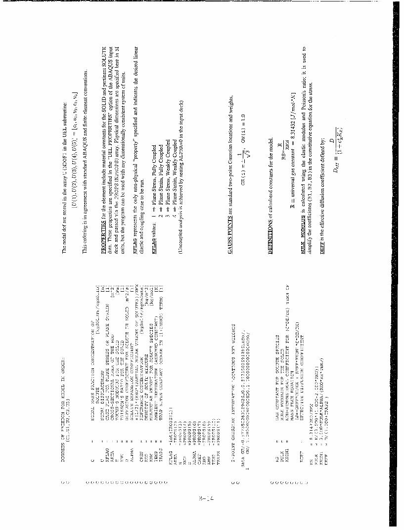
C)
a) a)
C/))
CIS cP) gCI 6
) LC),,a~ 0 o4
L) C) o 0*
or u4~ C r- M r-
a) C)i U )
C)Q p))C C) )
`2 CC) w~ o
1,11H 0 1'-r-~ C)C) ~r
0- C) U00E
0 0 )) ~C0- C) UC) ;4> C
I.-C C, Q El n- wU0
E) 0 11 C) 4 C) .0 Em In H C)ý 0 l
W.0C 0 ;7ý 0 U) U) C) CEl 0 x C) x) , E)El C) , : 0ý
C) 41 o W) CEm C)0mC)0C 0~ p x 02 Il CO El0 ý
m~ 0) C) C): W) U) 00 ~ -1-CC)~~ 0)C ~C
,h UC~) C, C) C) zC)` HNE :
t-i C4 0C C Z) r) oM) C) c) o )- D E )C C)HU W -E 0u 11 1-W U) W M W 40 ,
C) c14)C C)0C)0 11
CO
a4 N N '-4 a4 fC C 00~4 0- C0000000)
C) if - 0 C C) 11 1 1 i 1 1 E t 1 1 1
C) CD U)C'C4-- C-- 4 HL C) U)C 0 C-'I
E) H - - E, UU~ CC) X l l m
-1 C) C) C BC)14
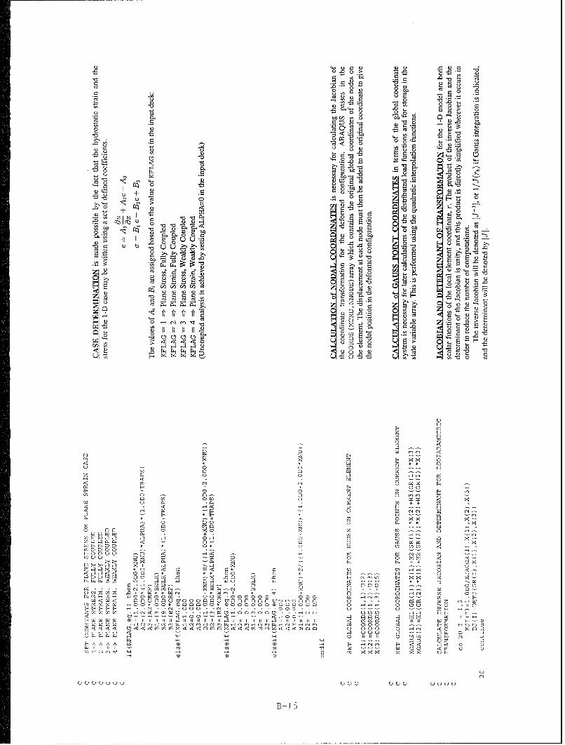
0ý Os 0> -5 0
La~ r- -0 .0~ g
0 0 b" 0 r-
o0 -0 0 0.0~~ 0+- H
>a '0 0.z
0~o 0 a1 ~0
.0 .10 ~ .
2 ~ 0 04 0~
0 0~
0j u 0ma 000 0
''I- 1 0
.0 0 + 0 0 .0 s
rA 0 =0=0 -00I *~
0 0 C
A 01 0000 0 o
'E -8
.00~ ~~~ 0 0 0.00
luý0 a 0
.00.
0 .
00 0ý 2
.0 CI 'I",tZ0..H .o o
00 00
0 0z
N 04
LO E- x x 0
000 0 0 o
+ ++ 0E;0 0 -l
o 0
04 IL 0 0000n n0 00 -4 H 0F, U *0 0 0u 0 0-
m2 U. 0 U 0>1 .2 0 1) 0 N 090 04- 0 0-
0a0 ) '0 * I. 0 -, 1 m) +I i H w 0 0 011.00)00)11 ooo000 00 -0 00 0 . 000 0, .- 0f 0 *
Wf):Q o o w o o ý 0 -4-H- 0 (D00 0 11
Hl 0 0 0 0- a) iti t i t 1 I t I t 11.2 11 I t 11 It 0I 11. 11 11 1 I t I 11. '- '1 '1 it 11 11 [1 0ý 0ý 0ý II II 0. 0 ON C H OI f4- lýýI O)1.-,O'14-I OIN 0 000 0 El-. H H h IDID:
14C 4_ Mo ýc< mc 0 000 0 -10 0 00.2.2.22 0 - .2 U U .2 1-- 2U0000~~~ X2 Q r 111 0 0 0 0
HA A A A 00 )a - 0 0 0
w0 a) a) CI
B-15

E r0
00
~.4,) 0 4
"0 0 CAý .
,,~ CL ,OIp 4 -cI
u0 _ 0.. A
E 4'
"0U .0.
=. A. - .0Z31
-. to,
0~ oui 0
0A
C14C
A- A wA A.
A A A.CA A E)jA A 0)A - - 4 0A n - -A - -A 0C - - 0 -0 - . -A .A .A A .
A 0 0 0 0 A C) IA A o. . o. . AA AA 44 44 44- ~ -. A 0 . ----. ~ 0 0
A ~ ~ ~ ~ I F-,-0 0 0 4.~ .A N'-, *4 .' 04-1, -Q)c - - - - I - - o - - N -
A. -A. A. -. -<CA .A ---. 0-- --- ---I- ~ ~ ~ ~ ~ ~ ~ ~ ~~~~U hO 0 O h . A '-.- -A--- '-.- - .
A.E ' 0 'C) A . -ON -1 0 -o A - 0
A. -- 0 - - - A.ý -ý 0 0 0 (CC')' 1:N 00 - 0o A. A. A. A. '- W I0-- -C.-. H0- -0-H--I 0
A. A. C 0A+.0A 0A0 . 0.). 0 A.0 AH) 00 0) +0 0)0 A. A. 00-- 24 0 -r - 0- 0 -A . -- '. ' . ' . ' .
+) +A A A A .A -0- '-- -0- "--
'C 00 00 w0 00H 0 - C -- -0m ) -0 -- -- E-l. ' . o .A. o .A A0 . 0 .A.D A. A. . 4F O 0 O-- O 0 h
v A. 0- 0- 0 - .- A .'-- A -- A--- A----(F H -- - - - - < .A 0 0 - ~ -N ~ N 0
A~~~~~~~~~ uC 00 00 ON 00 C A 0 0 4 0 0 0 ' 0v 0 - 0- 0 -- 0 0Av.- .- 0 A0- .-VV -- A. -Av-. -A ) A -0 A44 .H .44 A40
0 C) '0 '0 ' 0Cu) ) 0 h .h .h . h4-~ 0 'C a)- wC C AAZ 0AAA ~ . AA
'C 0 A.0 00 00 C )~ 'CA. 0+0 0 0 '0 0 40
A) C) 'C A. 'C A. C) uA 0 0 'CA A. 'A+ .'u± . 'A
A ' 'C 'C C - A.. A A.. A A.. ABA..1A

0 0~-
0 0
0
C,0" C
0-
0 ~
u .0
S -0
14 DCý -P r ý ýu)C- 0 2) 0 C
El ---
CD 0 0
00~~ eCC~j
CC0 13 0
In m z 0ý 0 0 00l E-- - - - C C C
0~~~~~I -H00 0 0 =C
H 0 u u- u C--- C- 0o IA 0 0C ~ ~ ~ ~ ~ ~ ~ ~ ý C - -- - 0 -- 0 - 0 -
xa- a- x- x --- -0 x xx
IA u 00 u u ~ u u 0 C
0 -0 --- 0 -- 0 CC I -C -C1 C-7- C -- a -

EID)
0 D
e,))
CIS
CC400
< 0 0
cl C2,
Q) AC UCCCU
0 Aa)C A
oCU) 0 )
<C ~ CC0ý C
~~C: El-C
C-C 0
El ý M E D nM D ýD
11 C kCI) 1 1 1 1 1 1 1 1 1 1 1 1 1 1 1
rCCm C) u
CD llý
OLD .1
C) U()UU u uuuuu u C
A -- B 18

0 0
0 A v2C4 0
>1 >1 -1
- 0D.-[
2 -d "c 0 w~04
=-t0 >
-E C C
0C H
v )
0 0E-- ~ C
= " -8 o -c
Eý E 0
m 04
> b,9~~ -4o -
0.
c .
A=0 C-CCOME
A OZ n Q 00A -000 El F-al.A El~H HZPA -< r40 ' W toHA 00 ElX 1 0 Lo0A D H0 OF-N .A S2 H i w0 0
A W4 0000 u 00
A cn w- w 0 n f4A l Z- ý0 w 0 EH
w 0 c0 E 0 PI
0000 00 OH00 0 P-
0~~~~ E 000HOEl Wo U E E
II HZH 04 W 0 a) -
[4-P0 0 0 u- HD C -
00 0E0 E O O0m ,00 m 2~
w O 0 UO 20 PHH +Dý ' ý
v N 00 ý .00 00 Hv ZI PC H aO 14 H ý-. H0 OZ 0 00 HOHO
H 0 C H 00o0 n01 1v m 0 0 OH 0.00
0 pqEl 0MP
W.0 0 0H
m 0000 0>1 u ul.-
0~~~~~~E (Z021 HO01 . 20 I
v 000OH Z O - oo- Buo 19

4'-' 44-40 44'
0,0 C
C4C
0 ' -
-0 ray~C,
bE~I I ZD4E(0~ý 4- ,4-4 .'t ý
CD '0D -.9 0)-0
f:14'~~04
I4 ¾ D uB u u u
C4 CO E4 C4 Q
(0U uO u4 u4 *N u- . u
I * B. 20

-~ E
C) Cd
oz u
C C- E
b >-1 12
00
o~~~~ r''10
"C -
CCC L
- CaCa It
A 77:C) 0' C'AC- -ACA
A a- -ACCC D MCM
A ý4 ý4 ýA x x xA-
C C)~A
5C):H -ýU C )C1 CCaC4ý4 ý
S'~cl 0 - -E
0' ~ Ca
114a
t4_ _ C_____'C-C
0- . I-- -
CC,, El
El <~I CCý D D Dý
A -''- -
v' 4
Ql) C' A El H lE NE ýE ýE ýH E
a(uj Au u u u uu u u u u ZN
1-)Ba2A

o cz oý
0 4s
04 C) W) rI)0
(0 -0 1- F1 a
10. .0)F0
LL0 - c C
>.( *04
-~ .0 .00- ~4 0~-
a) -i
ccc~ o -5c0
c z t> 2 'c .(5- a 0) ~aC
Z 0 )~- 0)C
> to
0~ coy -ct
o LI C)I
o ~A o c, P4 ~ c
F-F
FQ < oo
O -c --r 2l -
C) ~ 0 0>-~ C~t0 'c
CAA
A FDC)0 )0
A LOA (-IC-A w4mA Ad[-
LA
0 w10
c-A 0(4 EA ~ E Al 4111
.00 Q~O
0) C)' u-F FL
ccl w
00 A-100
11L Cl
LA 0 w4 Ao LA(4 fL 4 =11.00 r4 1 m)o L 0LA
C) x 1A C 0)40)1. 0 0~~ 0 -. c~AL
C) u A GALAu u.LC -L
F LA LA)L B-22

-l -. 0 0*
0 E 70aC
UI.0 .") . C
I: E -500
Q1 0 1
o S 0 oU0 0
+) U) C), CY
~c -0 E~~'-C---
u o, ~ :'EnC
I~' 0 -o
-~~D 040 -
,11 ~F- I
-D -fl ýD:C--~~~ý '--: x-~ --- ~~0
-0 ~ u
00 o
o0 ~~E EHHQC )
0 ~Q~C-' ~ F)7C
<~~~ -u C) U.
Q D 'ND H HU u 0. n
ý14 ý4ý4 ý4Ax x x IxA
oý Pý f4 A
cn
H H 0
0 (N ( 0 (Nm
0 - U 0 u u
B-23 * 0

03 0
bi)0
C)0
o :3'cz u
10
0 0
D ccu
0 o0
> to0 v ) ).0.
0~~= o. . ci 0
0 r.2. cn 0s 0
cn -4
0~rn -.- '~~C)~~ +~ . )4 0
0 ~ q
C4c
U) -0x~ El
m g0
wL coU) M
El 0- 0"0
0o - -0<Co 0-1 .010
KC) 0.
ElL oCf) 00
AD i<cf 100 w0 T1U
A CD 01 00A i--Cv C5 U. C40 mA - '- CD --
A -0 -0 u uu
A 0" ocB-24

r
0 0
00
0 7;
C 0
.0
0
E- E- C)
00
-'l +0 +
>i 10- C
0 ~ 0
IID
0
.0 U)CQ
F - - :1 - ,-H .El m 00g ,4f 1 1.
C) U1ý 1 It u r X -w u(1 ) 1 ) a 1E )Q
1-0 ~ ~ 4 Q0
000 0 a)7i7u Q 0 Q Q 0 0
0B-2

.0>
0*
0 0 0z
a v
10
0 0
0 0. 0) 0 .1) I1 0 .+0.1 11 .-0 0.4 +9
r4 I + 044, P>0,0u -,--- uI uI U) 0 u
0.44
C, -0 a) . 0 .0 09- a) 00 0 0 I 0-q-0 -7 Q 4 0 a) Tj ,a
0 oo u u0 .0 U.0u
B-26 4 ~

-0- -C CsE 0 >-2 -a r0
0 F- . 0O .= .9o>0 Hb.S b'd~ >7> 0
E CC 0CO 2O3 9 o 0
0~~~~~ >~00~~0.t
m H o . t') -o = ~Q)a 0 " -~ 0 .- o .0 00
>- *0 >d0' C/)~~ ~-
-0 C.) --.
cd 0 = _ 00
0C)0C 00
-0~ 0 "C 0 00
-. 8 00 C0
a. It o 00 0 m Z'E0 d OCg C=Od) .0
,0 o -00."".ol 0000- a. .
-0o~ o 0a.0 "a = a .0 E
.2 ~ ~ E ý.20
Z~~ ~ ~ 7L t0 L C00
F C
C")~ ~ ~ r400- l0 ~ EH7
0] .200W 0 00 ' n
r. -D -H 0 00 ,0 00
HO 0oE. 7 00C
F~0000 >
00 0 00 0,Z.2-
00 F
q 0 0
CC~ C-C 0 E
H H 00 0 00Z0 >C- 00 0 o
0 H F 0 oH E
E- 00
o~~~ 0.C0 C~0
C) 1- n0 0 0F 0 0w Q
0 C 0 PQ 0 w
CF4 N0 0-0F4 E0 0 C 0 0
Eo H1 x 0 0 HCI 0 w
0 0. 0 0E 0 0E0 C4D- N 0 0 00 0
E0 n 0+
0~U 0 > 0 00 H 0
Fl u00)0 0 0N C
U0 00.- U) Q 0 m 00 U
0 o0 o 00 0 0
000 00 0000
13 2

APPENDIX C: Sample Input Deck
This Appendix contains a copies of the ABAQUS input decks that were used to solvethe Case la, 2a, and 3a problems. A section-by-section annotated listing is also included.
C-1

ABAQUS Input Deck: Case la
*HEADING, UNSYMMSTATIC DIFFUSION -- STRONGLY COUPLED Standard Case 1
** C(0)=0.0 C(L)=1E-6** //** ---------------------------------------- F(x)70** //
** U(0)=0.0 t(L)=0.0
*PREPRINT
*NODE, NSET=ROD
1,0.ODO21,0.10DO*NGEN,NSET=ROD1,21,1*USER ELEMENT, NODES=3,UNSYMM, COORDINATES=1, PROPERTIES=11,VARIABLES=9,TYPE=U1** THE FIRST AND THIRD NODES HAVE DEGREES OF FREEDOM IN CONCENTRATION AND** DISPLACMENT, WHILE THE SECOND NODE ONLY HAS DISPLACEMENT DEGREES OF** FREEDOM. NOTE THAT CONCENTRATIONS ARE TREATED AS TEMPERATURE D.O.F.i1,i
2,13,11,1*ELEMENT,TYPErUl,ELSET=SCID1,1,2,3*ELGEN, ELSET=SC1D1,10,2,1,1,1,1,1*UEL PROPERTY, ELSET=SCID** PROPERTIES ARE IN THE ORDER:** CFLAG,AREA,E,NU,D,ALPHA,CREF,RHO,** MW,TEMP,TRAPS1.0D0,1.0D-4,200.0D9,0.3D0,1.0D-9,5.2D0,0.ODO,7.8D3,1.00797D-3,293.ODO,19.ODO*MATERIAL,NAME=A4340*DEPVAR
9*BOUNDARY** ZERO DISPLACEMENT AT LHS1,1* ZERO CONCENTRATION AT LHS
1,11*INITIAL CONDITIONS, TYPE:TEMPERATURE** 0.0 INITIAL CONCENTRATION OVER ROD LENGTHROD, 0.0D0*WAVEFRONT MINIMIZATION, SUPPRESS*STEP,INC=I000*COUPLED TEMPERATURE-DISPLACEMENT, STEADY STATE0.005,1.0, ,0.05
*CONTROLS, PARANMETERS=FIELD, FIELD=TEMPEPATURE
5.OD-21
*NODE PRINT, SUiMARY=NO,FREQUENCY=100
COORI,Ul,NT*EL PRINT, SUM4-ARY=NO,FREQUENCY=l100
SDV*BOUNDARY** SPECIFY RIGHT HAND BOUNDARY CONCENTRATION AS 1S0E-621,11,11,1.OD-6*END STEP
C-2

ABAQUS Input Deck: Case 2a
*HEADING, UNSYMM
STATIC DIFFUSION -- STRONGLY COUPLED Standard Case 2
** C(O)=0.0 C(L)=IE-6** I1/I** // ---------------------------------------- F(x)=0** // /
** U(O)=O.O U(L)=O.O
*PREPRINT*NODE, NSET=ROD
1,0.ODO21,0.10DO*NGEN,NSET=ROD1,21,1*USER ELEMENT, NODES=3 ,UNSYMM, COORDINATES=1, PROPERTIES=11,VARIABLES=9,TYPE=U1** THE FIRST AND THIRD NODES HAVE DEGREES OF FREEDOM IN CONCENTRATION AND** DISPLACMENT, WHILE THE SECOND NODE ONLY HAS DISPLACEMENT DEGREES OF** FREEDOM. NOTE THAT CONCENTRATIONS ARE TREATED AS TEMPERATURE D.O.F.i1,1
2,13,11,1"*ELEMENTTYPE=U1,ELSET=SCID1,1,2,3*ELGEN, ELSET=SC1D1,10,2,1,1,1,1,1*UEL PROPERTY, ELSET=SC1D** PROPERTIES ARE IN THE ORDER:** CFLAG,AREA,E,NU,D,ALPHA,CREF,RHO** MW,TEMP,TRAPS1. ODO, 1. OD-4, 200. OD9, 0. 3D0, 1. OD-9, 5. 2D0, 0.0D0,7. 8D3,1.00797D-3,293.ODO,19.ODO"*MATERIAL,NAME=A4340*DEPVAR
9"HBOUNDARY** ZERO DISPLACEMENT AT LHS1,1
** ZERO DISPLACEMENT AT RHS21,1** ZERO CONCENTRATION AT LHSi,11*INITIAL CONDITIONS, TYPE=TEMPERATURE** 0.0 INITIAL CONCENTRATION OVER ROD LENGTH
ROD, 0.ODO"*WAVEFRONT MINIMIZATION, SUPPRESS"*STEPINC=1000"*COUPLED TEMPERATURE-DISPLACEMENT, STEADY STATE
0.005,1.0, ,0.05
"*CONTROLS, PARAMETERS=FIELD, FIELD=TEMPERATURE
5.OD-21
"*NODE PRINT, SUMMARY=NO,FREQUENCY=100
COORI,U1,NT"*EL PRINT, SUMMARY=NO,FREQUENCY=100SDV* BOUNDARY
** SPECIFY RIGHT HAND BOUNDARY CONCENTRATION AS 1.OE-621,11,11,1.0D-6"*END STEP
C-3

ABAQUS Input Deck: Case 3a (Low Trapping)
*HEADING, UNSYMM
STATIC DIFFUSION -- STRONGLY COUPLED Standard Case 3 (200 elements) LOW TRAPPING
** J(4.0E-5)=0.0 C(L)=1E-7** //**------------------- F(x)=-1E6/(x+eps)^(3/2)** //
** U(4.OE-5)=O.O
*PREPRINT
*NODE, NSET=A
1,4.0D-5
*NODE,NSET=B
401,0.10D0
*NFILL,NSET:ROD,BIAS:9.470049D-1,TWO STEP
A,B,400,1
*USER ELEMENT, NODES=3,UNSYMM, COORDINATES=1, PROPERTIES:11,VARIABLES=9,TYPE=U1
** THE FIRST AND THIRD NODES RAVE DEGREES OF FREEDOM IN CONCENTRATION AND** DISPLACMENT, WHILE THE SECOND NODE ONLY HAS DISPLACEMENT DEGREES OF** FREEDOM. NOTE THAT CONCENTRATIONS ARE TREATED AS TEMPERATURE D.O.F.11,i2,13,11,1
*ELEMENT,TYPE=Ul,ELSET=SCID
1,1,2,3*ELGEN, ELSET=SC1D
1,200,2,1,1,1,1,1*UEL PROPERTY, ELSET=SCID** PROPERTIES ARE IN THE ORDER:
CFLAG, AREA, E, NU, D, ALPHA, CREF, RHO
** MW,TEMP,TRAPSi.ODO,1.OD-4,200.0D9,0.3D0,1.OD-9,5.2D0,0.0D0,7.8D31.00797D-3,293.0D0,19.0D0*MATERIAL,NAME=A4340*DEPVAR
9BOUNDARY
** ZERO DISPLACEMENT AT LHSi,i
*INITIAL CONDITIONS, TYPE=TEMPERATURE** 1.OE-7 INITIAL CONCENTRATION OVER ROD LENGTHROD, 1.0D-7
*WAVEFRONT MINIMIZATION, SUPPRESS*STEP,INC=5000,AMPLITUDE=STEP
*COUPLED TEMPERATURE-DISPLACEMENT, STEADY STATE1.0D-4,1.0, ,5.0D-3
*CONTROLS, PARAMETERS =FIELD, FIELD=TEMPERATURE
5.0D-21
*DLOAD,OP=NEW
SC1D,U1NU
*NODE PRINT, SUMMARY=NO, FREQUENCY=100
COORI,U1,NT*EL PRINT, SUMMARY=NO, FREQUENCY=l00SDV
*BOUNDARY** SPECIFY RIGHT HAND BOUNDARY CONCENTRATION AS 1.OE-7
401,11,11,1.0D-7*END STEP
C-4

ABAQUS Input Deck: Case 3a (High Trapping)
*HEADING, UNSYMM
STATIC DIFFUSION -- STRONGLY COUPLED Standard Case 3 (200 elements)HIGH TRAPPING
** J(4.OE-5)=0.0 C(L)=1E-7** //
** -------------------------------- F(x)=15E6/(x+eps)^(3/2)** //** U(4.OE-5)=0.0
*PREPRINT
*NODE, NSET=A
1,4.OD-5
*NODE,NSET=B
401,0.10DO
*NFILLNSET=ROD,BIAS=9.470049D-4,TWO STEP
A,B,400,1
*USER ELEMENT, NODES=3,UNSYMM,COORDINATES=1,PROPERTIES=11,VARIABLES=9,TYPE=U1
** THE FIRST AND THIRD NODES HAVE DEGREES OF FREEDOM IN CONCENTRATION AND** DISPLACMENT, WHILE THE SECOND NODE ONLY HAS DISPLACEMENT DEGREES OF** FREEDOM. NOTE THAT CONCENTRATIONS ARE TREATED AS TEMPERATURE D.O.F.11,12,13,11,1
*ELEMENTTYPE=U1,ELSET=SCID
1,1,2,3*ELGEN, ELSET=SC1D1,200,2,1,1,1,1,1*UEL PROPERTY, ELSET=SC1D
** PROPERTIES ARE IN THE ORDER:** CFLAG,AREA,E,NU,D,ALPHA,CREF,RHO** MW,TEMP,TRAPS1.0D0,1 . 0D-4,200.0D9,0. 3D0, i. OD-9, 5. 2D0, 0. 0D0,7.8D31.00797D-3,293.0D0,499.0D0*MATERIALNAME=A4340*DEPVAR
9*BOUNDARY
** ZERO DISPLACEMENT AT LHS1,1
*INITIAL CONDITIONS, TYPE=TEMPERATURE** 1.OE-7 INITIAL CONCENTRATION OVER ROD LENGTHROD, 1.OD-7
*WAVEFRONT MINIMIZATION, SUPPRESS*STEP,INC=5000,AMPLITUDE=STEP*COUPLED TEMPERATURE-DISPLACEMENT, STEADY STATE
1.OD-4,1.0, ,5.OD-3
*CONTROLS, PARAMETERS=FIELD,FIELD=TEMPERATURE
,5.OD-21
*DLOAD,OP=NEW
SC1D,UINU
*NODE PRINT, SDNMARY=NO, FREQUENCY=100
COORI,UT,NT*EL PRINT, SUMMARY=NO, FREQUENCY=100
SDV
*BOUNDARY** SPECIFY RIGHT HAND BOUNDARY CONCENTRATION AS 1.OE-7401,11,11,1.0D-7*END STEP
C-5

CIO
C))
C))
C, a
10 - z-"q -U) U)
u0 '0=*-
_bl 0) 11~U)U) 7*<--~ 0~E- ~EI
E 10.0 E cZ r
C.)0U) 0) U) f-
con CE ý0
U )03 E ) U
0 UD I~+
0
mU)
a-C-6

0 0U 8
d) Xl 0 *
c)~ ~ c) >
cc,, 0 E2
oc 0
0u 0 V ~ o o. C;O
u c) 9~
to 0
*0
,o 0.0~ )
cn r. u 3
= U) - a 0 ,5Z -0 4
00 o u
to~ ~~ 4 Fc:)U uC
40. 0 4CF
U- >9 4,5Um z-U
c) -cn a U)o o)U
CU c
-< E - q) U- <
C) ID 0 Zo
E C CDOr
U E
U)<
El~ m N o
U) FC
C- E-- W)U (:1U)2;
Cz C-) o
Co Q
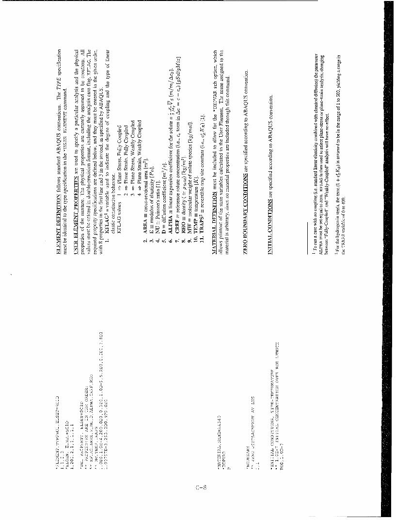
.0
o 0U 0 ,l;0 E*5
In Cal 0.
CO 00
LU) C) 5 0 .- ý
0CO OO >
~00 -0 o~-0
0WC 0 00 u-10
r o
rc 0-c U) CEO
C4- m~(U -c t.0 -8 z9 > 0'0 Cl o. oý ~C
00
C) 0U C,- 0
0"0
0"0
S 00 U AA0
0.
~~-,Q O0~
1 0O * C 0 00, O
CO 0,0 > II -
z: o w llu E,)
EO* 00
EC CU) w u-COD,. C-C CE
C-89
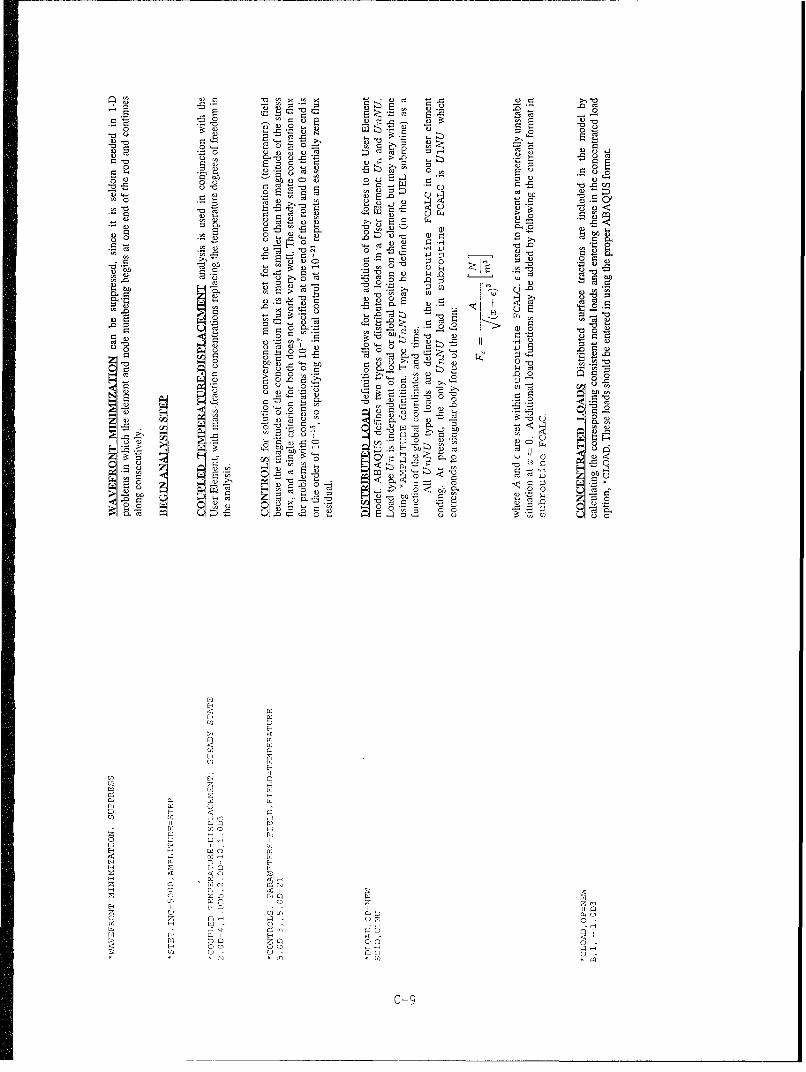
0~ o 8 ~ 0 -
0 .- 00*- 0.0
430 u0 00C c
o _w ~ E f
0s 0".0 43.0.o11 0>000 02 0 0
0.0 =0~0 -- o~P 2 r.0 ~ ~ ~ ~ P 0.0~C0.
0.
0o0 m c.o2
0 4J0ý: o 00
ooop 00 0 7s- *
~~.~ 0 00 0 00) . 0. c,
. 0 0~.
0~~' 1>~~ r 0 0.0~~ C :0)
0 0 000 0 - 0. j 495 G
0l 0 .4
r~0 .0 0 0 0" 00 0.oo
o00-) o~ 0 0.0~~~ = ~o- 0-
~~.05 ~ 0.o -000 0.0~ 0
01 00.
o.0 0= 00
Ur0 -0 +o. S). 00 q>~
r- 0 00 CD~o2 w 0
_0
m 00.c t0 0
a 00 00 0. 0b4Q z. m 20. 0
IIs 0. 0
a4 Fa-
0 0
0 0. E0 00.4
0 0 0
H~c) 00. '0El 00 1 0
0.0
F II (9 - . 11
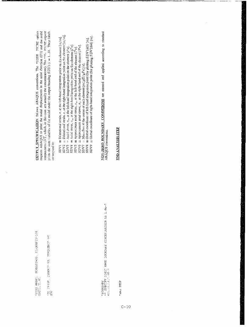
C r
ia4 HP, r 0 Q ýj ~ C-4 -
0 U
- 's -. C
o 4-EE c l ~
C z ~ ~ ~ c-d co-
>~ 0.
r- C)e 00 C, )
Q C
tn- CD VE .E Cý C/ cn Iu a
010
D4 D
C-1

APPENDIX D: Sample Output
This Appendix contains a copy of an ABAQUS output listing generated in thesolution of a 1-D fully coupled deformation-diffusion problem.
D-1

ulU)U
U)-mU) w E
QH m U) UH n U
wFU
w ý ý ý H nHHýElH
A A Av H I IH
HI IH H H -
v H H H v1ao o o C) H A A AO
CY0 Y A Al A AA A A A W lW
CY 0 - - - -- 11
II 00 V VI I EV V H
01 0 01I I01~ 01 0 A IA A A AAHIII
0 01 I I U VV O
010 A AI A A AAA I U
01011010010 v I I------------HIV II V V V ( H
AA A A AA A AAH0
A A A A A AAA(n
-- ------- (nHm QCQ vv I I v vv Hco
m o1 A AA A A A AH X
AA AA PQ
I IAAcoA AA
I H H -
H H H VV I D-V2

00
0-I;?; 0*
E H Hý H CHI',O 1W
El 0 .10
H -HH H 00 0
H l M Z~ HO HH 4H 0
ý HO< M E < iW 0 WE
HHH 0 H HD it HO (WW 0 E 4 10ýI
HO HO HH 0 H OHHHO H 0 H 0tiE
00 C)HOE
tO H H)ý 0 Q 0
HO 0 OHH 14 2 Nx EHw OC H : ; U> OH; OHm DHH H1 H-Hý u CMHH > HE E H
El~ O H 004 (n-E00:0 0 >,M 1
H0 H 0 : :OInO a 00 a *H 0 H 0
H :H H H >UiHO . u o H - H U ii >
00>C O H H-I-QiI H 2 <
oa 0 0 O HHH coOHi-i0 0 0-H

0'n
Il 0' 4 0
El 0
I momIEH In 0InIn
Q 00000~~ w 4'4'1 lO
0~~ ~ I ' '-0
H~m00 I4 4'
w'H 0
w>- I 4 El In U0
W11N 2 U I 00 1>0 nn I
"2 ~~~ El 4 I I >
ml w0 W1* W El U ~ lUo i al H Il: 2 a
m i1 0. i El 0"a w II OQ Im aU InI In C 000 0 Ini
Eo w I 0 CD co n W 0 0,u f1> ý0
0 ,n I 4 0
In' E, l0 G 0 o2 If4 I ~ I 4 0 0 n a o eOFInICO- F 0 . 1 00 0
4' I 4 "0 I - In O 0Ol~~ : In.2 InueO -O > 1l0m n i -0
a' i ' In~~l-4~ n 0 - ~

o1
In :D Z oI
01 'CI1
w o I I1
QD I x I4ý 2
H, ' 1014 4' I "t I H) H ,E
In0 0n w E0 [I ±Ht I I4 I H
0 0 0<I H'C I 01 0
EC 0 H, `I I Ho~ o I U E,1 , 4 E
o 0 .I nC ,D0CDI IU I
;7 0 E i II0 0 CD I o * m H11C) ~~~~ ~o ') WCn I 1 H 0 i I '
'C I onC In 0 0 E0 In 'I I 1 InI
HC I II In .2 .2 In[4D '
In o >1I u) H In 0 In WD En E1 In Q 0041r0~~~~~P IfF0)DC CD -' 0 nP! E I "I Hl I> toI C 0Z 0P- Io 020 F X0~~~~~~~~1 01 -n H In I-4C C 0 ' CI~
'C H O mD ' C o W W 'nIn H Cm InI H H- II o~t 'In CD C . IH'~~ ;E; CD41 0' ' I 04 O
In ' 'C H ~ n ' HO ' I 0 0 0101 EI >In~~ ' oD 114C In - I 1 ' F -- 00 D HF 0 F H F' 01C DD I~ Co ' O<u 0 DD - 0- ~C 11 0 ICD ' DOC O 0 CCI H - H >-I -I ' H >. S F 'o t±-
.2 OO DO .2 I H D n~H~ I '0 I C C-5.0

Em
El
0
00
> CDI 2V)El CEoE
m- 4119o~
On m uýM
FD-6

HýC00
00
00 In
(N 0
0 H ýH~00H 0
00
El 0 0
o 0
HO 0 >
0 0) w 0 0
H 0-N
40 H1
HO 0 cLOH0HWnN0H 'H7 EH HHH HH 0
O0 H Hr,rCO H 00 mP
El0 w 0 QC40E 0 oD oDnMý ný
r4" 0 0 H H 00l--
O0 0
~OZ0 H-H

o 0
E 4 4 E
0 E 04 4
El u0 C4
H ý
0 00(0
r4H a C
(: o 0 mfn aHa Hn
a a D-8

in
Ein. . . . ..-
F4W 1 WWW WWW4
iný
o~ in
@ 4 1 1 -14
Qo inýz
41 0
zn 00 000 w~r 0000 7-I r, u I I I I I
:2ý inni 0 nninin 00x0 w nioini0 0 0 0 0 0 000 0 0 0 0 0 0
El , 000 N 0000 00 000
En 0 a: . . . . .m 4C
in 0l 00 4n 0 ýr
o2 0 @4Eio a
f ,0 inE ý 0 1
in in a
in I EHC: l u w 4 w f0 inw
oJ~ o in in o00 2 C ýE t N EH in ini El 22 00 in
.24 0 H o oooo l n HOO @40 D.9040 F E C4 2000 4w00ýE 0 ý20 0 0
HO oa oao o~a ooaooo , D Nin on ri 0 0 i0 0 n
<4 0n .22 HO in W2 in 0rO u) p ut in n inin inPi i P n ni Din ý 4 p l noc
a~~~~cE 0 H-F 00 0EHD4 0 20 H
00 F.U OC in Fu0 iinn..............................i n0a : H
O O O O H H O H H H0 00000 @ 000 n i .2@ @4i
in0D-9 Z @iioi.>i

CD
H~~ ~ 0>02 0 0'0'o~f000 00 a-1
0 00 0
C4 U) wc 0 I E
0'0
z 0 ý H co 0
w0 El 0 0 (9 0 01 "
HO (4 Cc H U0 ) O H H U)(D 0 C- ) (9 00 DI U
U) 0 Cc 0 00 U) 0 (9 - ) (
'o [14UW 0 000 (90 (9 ( 0 c (9( 000)wE & ,E 0 0U) 0 0
0(9 a(U) 0 w HC) 00(900 E 4 H "n U) 0"H01rS
w(91) 0 w <2 l 0x 1 -1)
W> o Uo 9U 0 H- HH U C)0On 00 0 U)E w 0 oUE:( 00(9 :Z )
Cc U 0) 00 0(9U U) ICc(900 E-W0z U) ,E E09( 0 0H E HO (9 C)( 00 <04 OH
U1 U0 F140 00 U (9WCc )2S0 CH4 Z0 DE C '
00 (9D~ CQ m c 0000E0 E 0U c< <C )w0 O H( (9OO0<cOHOH m00 0 OH NO ý 00c m
ýr E 0 QO H 0l 0 1 0 0 0 0 0 H O H (9E00 2:n 0 0 f4(0 0(9( 00 0 0 C 0
0 m 4 x0 (9 9 01 -11;49 H00H( E 0, 0 1o0 w(9U)U)000000H000w
00 " H U (MU 0C F Pý E00P00 C ý
>H 9 o ) M00 00E W "0 0 HO H 000 Ip u r00. 0 9 :D90 000 U)0 0H 00 00 U)UU) 0(ME9E uuu;R
E~ 0 nOHHO(u 9 000000 0000 0000U) "C (9H 0 00po zH CcOHu HHH HHHU) o(OHIEOQ CcnE-nHOwOW H 0ý Hrný Hw0E00Z00 N 0EO
(9 ( 0 Z9cH 009(999( C CccýDcc HH(E-U HHP00 0 0' (99W0 00W0 0 0 O H H"IHlC C :)1 D1 4(
c0 040<
*EH
D-10

0
H /
El
0r
w EHHý
0' Q
w Hl(N0
H > Q QQ H P 0 H1
(n 0 C4 Q
H g
0 HDU 0) 0HD(
oH 0
HH En 0 H>H H 0
' O M H4 'COHE U 0
H C H
(0 HNH 0ý(-(w 0-1 HHQ H q Q 0
:D m H ' 0Ol C, 44 w
'C4 HnH wEHZ H U
HO HOD-11
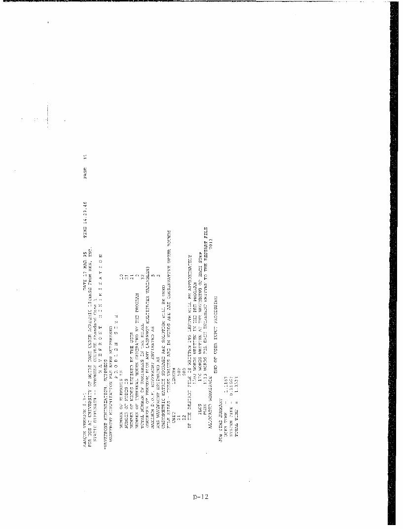
'C C
0.0
ml m
141
m0 r40 HCQ 24 CDH'01 H
'CW 01 N
Hý 0 HZ 0Z01 01 VN HNH0H 4
r)0k 0. > .2 U00f.m1n0C 02coN4' F, 'N P 1 Q4 U
C4 01Q -01 w 2 xZ 0110 1 Nz
z0110 0 'C H111 0Hk N Q 1 0 R O 0
wC al wH 01 0n CtA &I -0m 1-AN 001EC2 N0 C 0.N ' F4 .2' 0
In wm oc0 0.uE
.24 o m 010 - 0 R Z Z 0 0010 02 G Z~ H C~~00w 01. KC~1H 1HH H
012 01 e1H N 1 2Z N Z Z
01ý m m . ' N N mm 2 N - N H
Zm 011 0000F10
NR 011010N01 'F F 12 H

00000
OH 0110eU
;2n 00000ene H I I I
> e (4 t W eW tetEleC0 eeeeeme U H HH
'Cw H
Op ~ ~ ~ 0 0 0nnee0nne neeeHO nneee
0 00000l
-1 M H ennne
en En0i
uZ 00000)0 HH I EI
00 eneenne
en~ Ne 00 -enennen 1 0 00 HOOHH II
0 0 0 P O l
HO e H H 04ne H) 0 El W WW
EZ I H EenEoenenEH en en
A E Fen umen noaH.to 2a enW~ El ene m
e4 E0 0 H e O n n '
(eC H, 00 ~ e
en ~ E 00 H a n 11let ~ ~ ~ E enWee O > eeeee
0 a~en c e enD A 13 e
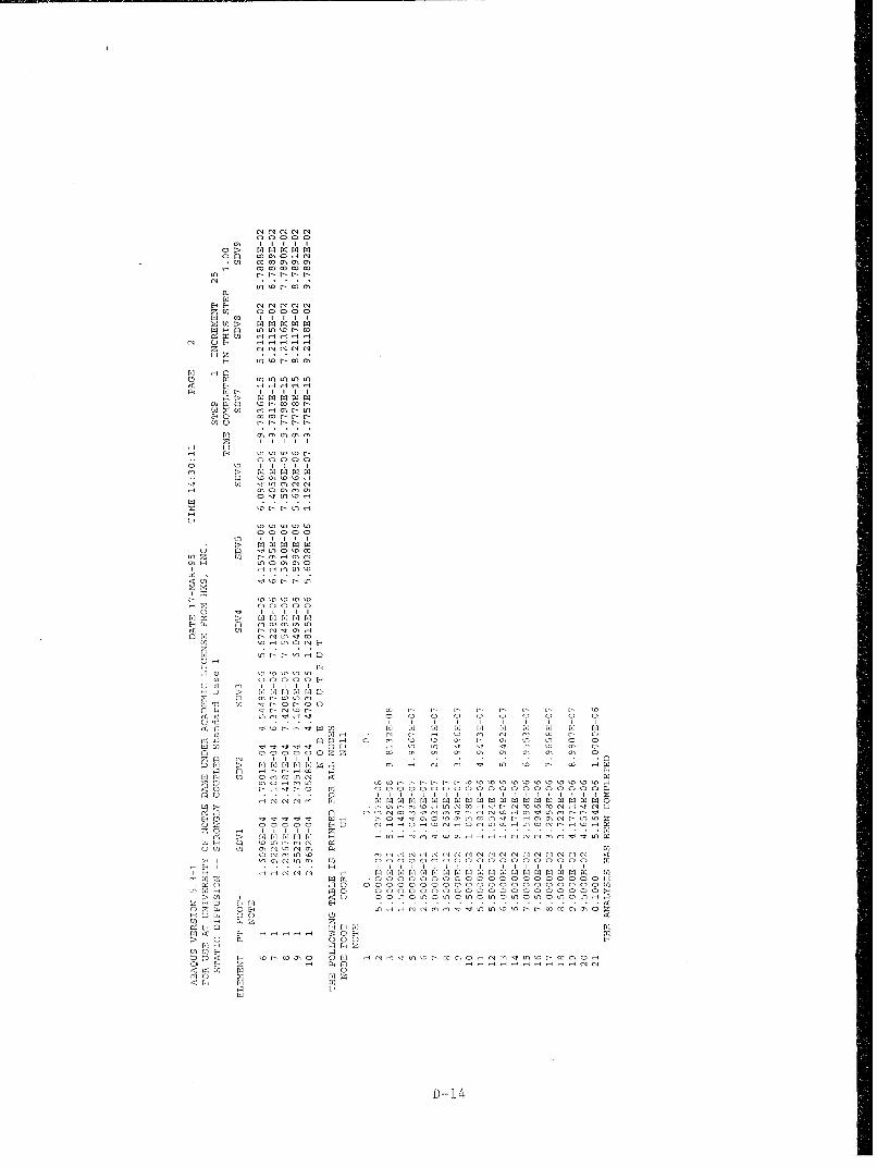
N 000
Hý 0 0 0to u N N
00 0
mo o o oro0H "I I 0NI 0
o HZo0 p o0 0
r HZ 4 0NNN
01 00 0
0 2 I- I E I I o
(4 H 0 00 0 No . o o o . ~ o . ý
f, 0000+
F2 4 0 NO
< Zl 0000
W H 00000 I
m0 0- I I I
002 C 0000
HO CD 010001
E,0
HZ
N HO
P Nul u
El.
0CO
El
C4
0 cN
01
C,
-D91
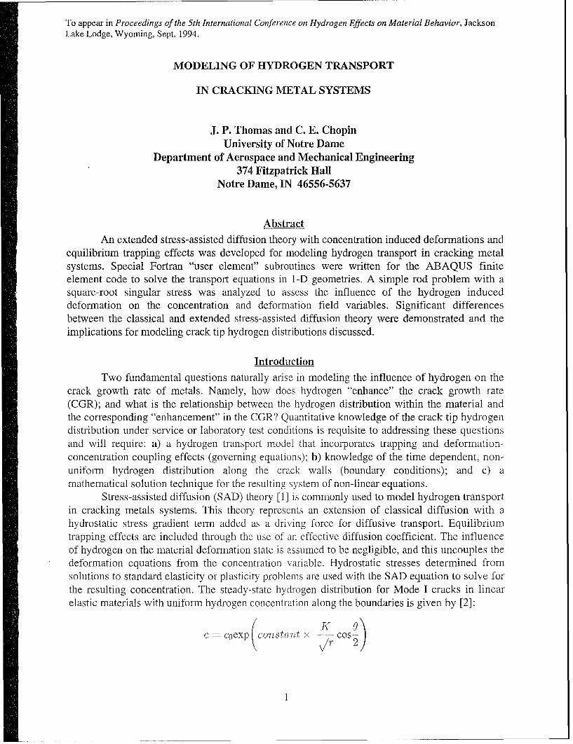
To appear in Proceedings of the 5th International Conference on Hydrogen Effects on Material Behavior, JacksonLake Lodge, Wyoming, Sept. 1994.
MODELING OF HYDROGEN TRANSPORT
IN CRACKING METAL SYSTEMS
J. P. Thomas and C. E. ChopinUniversity of Notre Dame
Department of Aerospace and Mechanical Engineering374 Fitzpatrick Hall
Notre Dame, IN 46556-5637
Abstract
An extended stress-assisted diffusion theory with concentration induced deformations andequilibrium trapping effects was developed for modeling hydrogen transport in cracking metalsystems. Special Fortran "user element" subroutines were written for the ABAQUS finiteelement code to solve the transport equations in 1-D geometries. A simple rod problem with asquare-root singular stress was analyzed to assess the influence of the hydrogen induceddeformation on the concentration and deformation field variables. Significant differencesbetween the classical and extended stress-assisted diffusion theory were demonstrated and theimplications for modeling crack tip hydrogen distributions discussed.
IntroductionTwo fundamental questions naturally arise in modeling the influence of hydrogen on the
crack growth rate of metals. Namely, how does hydrogen "enhance" the crack growth rate(CGR); and what is the relationship between the hydrogen distribution within the material andthe corresponding "enhancement" in the CGR? Quantitative knowledge of the crack tip hydrogendistribution under service or laboratory test conditions is requisite to addressing these questionsand will require: a) a hydrogen transport model that incorporates trapping and deformation-concentration coupling effects (governing equations); b) knowledge of the time dependent, non-uniform hydrogen distribution along the crack walls (boundary conditions); and c) amathematical solution technique for the resulting system of non-linear equations.
Stress-assisted diffusion (SAD) theory [1] is commonly used to model hydrogen transportin cracking metals systems. This theory represents an extension of classical diffusion with ahydrostatic stress gradient term added as a driving force for diffusive transport. Equilibriumtrapping effects are included through the use of an effective diffusion coefficient. The influenceof hydrogen on the material deformation state is assumed to be negligible, and this uncouples thedeformation equations from the concentration variable. Hydrostatic stresses determined fromsolutions to standard elasticity or plasticity problems are used with the SAD equation to solve forthe resulting concentration. The steady-state hydrogen distribution for Mode I cracks in linearelastic materials with uniform hydrogen concentration along the boundaries is given by [2]:
c coexp (constantt X /r cos0)

where co is the boundary concentration, K is the stress intensity factor, and r and 0 are polarcoordinates centered at the crack tip. An infinite hydrogen concentration is predicted at the cracktip. Transient and steady-state hydrogen distributions for a plastically deforming crack in ironhave been obtained by Sofronis & McMeeking [3] using finite element methods. Their resultsshow large, but finite, concentrations at the crack tip region, primarily in traps near the cracksurface. They conclude that the crack tip hydrogen distribution is primarily determined by thecreation of dislocation traps via plastic straining at the crack tip.
Damage models that attempt to link the crack tip hydrogen distribution to the fractureprocess have been reviewed in [4-6]. Applications to service cracking problems have met withsome success, but the lack of information on the crack wall hydrogen distributions under serviceor laboratory conditions has limited the usefulness of these models.
The task of specifying the crack wall hydrogen distribution is difficult because of thecomplex nature of the interacting chemical, mechanical, and metallurgical processes operativeduring hydrogen assisted cracking of metals (Figure 1). In aqueous systems, the hydrogenproduction process is driven by the rapid and irreversible evolution of the chemically unstable"bare" surface at the crack tip to a more stable equilibrium "filmed" state. An electron flow isinduced between the bare and filmed crack flank surfaces; net anodic (dissolution/filming)reactions take place on the bare surface and net cathodic (hydrogen reduction) reactions takeplace on the filmed surfaces.
Adsorbed hydrogen, Hads, can be produced on both the bare and filmed crack surfacesby: (1) the reduction of hydrogen ions in acidic environments; or (2) by the reduction of water inalkaline environments. The MHads species are then free to be absorbed by the transition reaction(a); or combine to form H 2 gas via: recombination (bl); or electrochemical desorption (b2).Reactions (a), (bl), and (b2) occur in parallel, but one of the two (bl) or (b2) reactions is usuallydominant (Figure 2).
Crack Tip RegionBare alocal
Steady State Film Coverage Film Growth Surface
MeT (Mie" . IHI, C1, Naet , .. )menH
ý - -
1. Electrochemical Mass Transport2. Anodic and Cathodic Surface Reactions local3. Hydrogen Absorption Reactions4. Hydrogen Transport and Trapping5. Hydrogen Damage
Figure 1: Schematic of the processes responsible for hydrogen assisted crack growth.
2

(1)Acidic: M + H+ + e- € MHads
(2)Alkaline: M + H 2 0 + e- < MHads ± 0H
(a) Adsorption-Absorption: MHads 4 MHabs
(bl) Recombination: MHads + MHads • H 2 + 2M
(b2) EC Desorption: MMHads + H+ + e- €:ý H 2 + M
Figure 2: Summary of the hydrogen producing reactions.
The distribution of MHabs along the crack surface is governed by the surface coverage ofMHlds and the kinetics of reaction (a) acting in parallel with reaction (bl) or (b2). These factorsare influenced, in turn, by: the electrochemical environment at the crack tip region (e.g., thepotential, pH, species concentrations, dissolved 02, etc.); the kinetics of the bare and filmedsurface reactions; and the rate of transport of Hab, from the crack surface into the material.
Iyer and Pickering [7] review and model the mechanisms and kinetics of hydrogenevolution and entry in stress free metallic systems with homogeneous electrochemical conditionsat the metal surface. Their model is used to quantify the rate constants associated with reactions(1) or (2) and (a) and (bl) or (b2) via analysis of experimental permeation data. Turnbull [8] hasreviewed electrochemical conditions in cracks with particular emphasis on corrosion fatiguecracks of structural steels in sea water. Similarly, Beck [9] and Newman [10] have examinedexperimental techniques for characterizing bare (and filmed) surface reaction kinetics. It seemsthat the above models, data, and techniques, plus information concerning the rate controllingprocess during crack growth, will have to be used in an analysis of the mass transport processwithin the crack to develop realistic predictions of the MHads distribution.
The objective of this paper is to address the above items a) and c). A hydrogen transportmodel for isothermal linear elastic materials with mutual deformation-concentration coupling andequilibrium trapping is developed using continuum mixture theory. Computational solutions for1-D geometries and arbitrary boundary conditions are obtained using the finite element codeABAQUSI supplemented with Fortran "user element" subroutines. The code is used to analyzehydrogen transport in a 4340 steel rod subjected to a singular body force( --, A/x 3 /2 ) whichproduces a square root singular stress. The concentrations, displacements, and dilatational strainspredicted by the fully coupled theory are somewhat larger than those predicted by classical SADtheory, depending on the extent of trapping. Further examination of the fully coupled theory inthe context of hydrogen transport in 2-D crack systems is currently underway.
The paper begins with a description of the strongly coupled hydrogen transport model.The use of ABAQUS with its "user element" subroutines for solving 1-D problems is describednext, followed by an analysis and discussion of hydrogen transport in a rod with a singular bodyforce. Extension of the finite element model to 2-D geometries and its application to crackingmetal systems is briefly discussed, followed by suggestions for future work.
I ABAQUS is a commercial finite element code supported by Hibbitt, Karlsson & Sorensen, Inc., Pawtucket, RI.
3

Modeling the Hydrogen Transport and Trapping ProcessThree species of hydrogen are modeled in the analysis:
HL -- interstitial or lattice hydrogenHR = weak or moderately (reversibly) trapped hydrogen (e.g., AEb < 30)
HI -1 strongly (irreversibly) trapped hydrogen (e.g., AEb > 30 kJ/mol)
Balance EquationsBalance equations for the mixture mass, the three hydrogen species masses, the mixture
linear momentum and moment of momentum, mixture energy, and mixture entropy can bewritten. Since our modeling considerations are restricted to isothermal linear elastic materials,only the balance equations for the hydrogen species mass and the mixture linear momentum(assuming negligible inertial effects) need be explicitly considered. They are given by:
Mass: 0---+ V -Jk = ak (k=L, R, orI) (1)a9t
Linear Momentum: uij + F = 0 (i,j x, y, or z) (2)
where: Ck - mass fraction concentrations for Hk [kg/kg].
Jk concentration flux vectors for Hk [kg/kg r m/s ].ak mass supply rates for Hk [kg/kg/s].
caij stress tensor [N/m 2 ].
F- the ith component of body force vector [N/M 3].
Trapping AnalysisExpressions for the mass supply rates ak in Eq. (1) are written in accordance with the
trapping model of McNabb & Foster [11]:
Stoichiometry: HL €# HR and HL =- H1 (3)
The stoichiometric relations require the supply terms sum to zero (i.e., aR + al - aL).Kinetics of Trapping: aR = k~f(1- OR)CL Rk•O (4)
k{(1 - O,)CL - k I01 k -(1 O,)CL
where: k{f, kf, k b, k b = forward and backward trap rate constants for HR and H1 [1/s].0 R and 0, - cR/c 8 and c_/cs, respectively, are the fraction of filled trap sites [1].cS and cs - saturation mass fraction concentration of HR and H1 [kg/kg].
The quantities kf, kf, kb, kb, cs and cs are related to trap site densities, probability of capture,etc. and can be determined from experimental measurements (e.g., [ 12-14]).
Significant simplifications are effected when the rate constants for trapping are muchgreater than those for diffusive transport. Trapping can then be modeled as a steady-state process(i.e., aL = aR = al = 0). This case is considered below.
4

C8 KR CLSS Trapping: CR -- 1± KR CL & CI = c4 (5)
kf - xKR R= xp AEb)
so that the total internal hydrogen concentration is simply a linear function of CL(Xi, t):
CTOTAL(Xi,t) = CL(Xi, t) cR(X,) +cI(Xi, t) = (1 C KR)CL(Xi, t) + c} (6)
The three versions of Eq. (1) can be summed to give a single equation by the followingconsiderations. First, JR = JI = 0 because of the linear elastic material assumption whichprecludes trap site motion (e.g., dislocation motion during plastic deformation). And second,from Eq. (5a):
9CR DCL OCIF;•ý CsKR and t 0 (7)at R at at
The resulting mass balance equation is given by:DgCL
(1 + cs KRa)C- + -L = 0 (8)
Constitutive EquationsMass Flux: - CL DL VAIL Linear Onsager Relation (9)
RL T
where UL is the mass based chemical potential [15] defined by:
PL 1 (p°L(T) +RTln(CL) -VHke) [J] (10)
DCL ML L jand: DL diffusion coefficient for HL [m2/s].
RL gas constant for HL = R/ML [J/kg °'K].
ML =- molecular mass of hydrogen [kg/rnoll.
T - temperature ['K].
0 - V)(CL, CR, c; cij ; T) free energy per unit mixture mass [J/kg].
LP'(T) = reference potential for HL at temperature T [J/kg].
VH = partial molar volume of hydrogen in the metal [m3 /mol H].
k bulk modulus of elasticity [N/m 2].
e trace of the strain tensor (i.e., e = ii = Ell + E22 + E33) [M/m].
The use of mass based chemical potentials simplifies the analysis of fully coupled deformation-diffusion processes because of the primary role played by mass in the deformation equations.
The resulting expression for concentration flux is given by:
JL DL VH DL kCJ76 (11)
5

The constitutive equation for the stress consists of Hooke's law combined with adilatational stress contribution due to changes in the total hydrogen concentration:
Stress: piJ ao A e 6ij + 2Gcij - 3 k ceH (1 + c' KR)A cL 6ij (12)
where p mass density of the solid [kg/M 3].A Lame' constant [N/mr2].6ij Kronecker delta (•ij = I for i z-j and 0 otherwise).G shear modulus [N/mr2].6ij i1 (ui,j + uj,j) infinitesimal strain tensor [mrn/m].
ui --the ith component of the displacement vector [m].iH- linear expansion coefficient for internal hydrogen K VH [M/n/AcH].
(1 + c' KR)ACL -= change in Ctotal from some reference level.
The relationship between the chemical potential and stress (Eqs. (10) and (12)) is dictated by thethermodynamic reciprocity relationship:
D -/L _ (u7i/P) (13)acij DCL
Governing EquationsCombining the mass and momentum balance equations with the constitutive relations
results in the following system of governing equations for transport:Diffusion Equation:
OCL Deff V 2c- VH Deff LV2 (14)
Deformation Equations (i = 1, 2, 3):
(A + G) De +G7U+ ,=3 l(+c'KR) OC (15)x R (15±
where Doff is an "effective" diffusion coefficient defined by: Doff _ DL/(1 + c'KR).Equation (14) is identical to the stress-assisted diffusion equations published in the
literature with the exception of the V2e term which is identically zero when linear elasticmaterial behavior is assumed (and Fj = 0). In the present formulation it is given by:
3•2 3kcrH (1 + c' KR) V 2CL (16)A + 2G
Computational ModelingEquations (14) and (15) form a system of non-linearly coupled partial differential
equations that must be solved for CL and ui as functions of the space and time coordinates (xi,; t).This is accomplished for 1-D geometries by writing Fortran "user element" subroutines for theABAQUS finite element code to effect a computational solution. The 1-D "plane stress" form ofthe governing equations 2 (aor =Y Cz7 = 0) is given by
2 "Plane strain" forms of the 1-D equations can be obtained by a simple change in constants.
6

&CL OJL _0(7Diffusion: (1 + c' KR) -O 0 (17)R at ax
S OCL VH DL OJL ~DL + VHDLkae
a9x IRT ax
Deformation: O + F 0 (18)
Ux 3k(e- 30H (1 + c'KR)A CL) = (a (1E K) )
A single differential equation for CL can be obtained by combining Eqs. (17) and (18):
OcL a F 1 (I +cOK\)CL VH DffLat x [ff MAL R T -R ) ax± 3RT FxcLJ (19)
which, in the absence of body forces, is a standard diffusion equation with a concentrationdependent diffusion coefficient. Solutions to the steady-state problem, with and without bodyforces, can be obtained by integration (symbolic computation is highly recommended).
A coupled set of equations for a single finite element of length h and cross-sectional areaA can be written from Eqs. (17-18) using the method of weighted residuals. The result, afterintegration by parts, is given by:
oh (( + C KR) { x -- Gi(x) d=- h±~R) at fi.x~ J axx)}dx= -J{Gj()} 0 (20){G JJ(xL){} x}-0 (20
-ux o ax _F {H3 (X)} dx= -ux f{Hj(x)}
2
where: CL LGi(x)ci(t) LG (x) {ci(t)} Z-- 1,2 (21)i=1
3
u L7Hi (x)uj =LA J f j VI j 1, 2, 3j=l
are 2 and 3 node finite element representations for the lattice concentration and displacement,Gi(x) and Hj(x) are the respective linear and quadratic interpolation functions, and '"indicates a row matrix while {... } indicates a column matrix.
Substituting Eqs. (21) into (17b) and (18b) and converting to isoparametric coordinates,results in finite element equations of the form:
[ [C]1 [0]1 V{iI} [Kc] [K,.] {ci} {'c([0] [0] {'d I L [K,] I{R} (22)
The capacitance, stiffness, and RHS matrices, [C], [K], and {R}, are functions of CL and u,which necessitates the use of nonlinear solution techniques. The integrations required for thecomputation of the [C] and [K] matrices are accomplished using two-point Gauss quadrature.
The term Oe/Ox in JL includes the second derivative in u (from Eq. (18b):
'7

_±e 1- 2U 02(23)ox 2v)- + 2(1 + v)aH ( + R OCL(x
This would normally require the use of Ci continuous elements in order for u to satisfy theelement interface compatibility requirement [16]. To avoid this complication, we use the valuesof u and CL from the previous time step to approximate Oe/Ox in the current time calculations.
The deformation equations are analogous to those of linear thermoelasticity. This allowsthe use of ABAQUS' coupled temperature-displacement routine to solve the problem. Timeintegration is performed using an implicit backwards difference scheme. The computations andsetup required of the user element subroutine include [17]: calculation of the [C], [K] and {R}matrices; calculation of the "Jacobian" and {right-hand-side} matrices for the Newton-Raphsonnon-linear solver routine; and updating the solution dependent state variables: JL, o, e, and&e/Ox. The subroutine is written in double precision Fortran, and the code is run on a SunSPARC 10 workstation.
Applications
Steady-state hydrogen transport in a 4340 steel rod subjected to a body force selected togive a 1/xV singular stress (Figure 3) was studied using the ABAQUS code. The rod wasdiscretized using 200 elements of length 1i = 0.104/0.94'-' [Mm], where the first and smallestelement (11 = 0.104 [/[m]) was placed at the left-hand end of the bar (x = 4 x 10⁻³ [cm]). Theparameter values used in the analysis were: p =7.8 [g/cm 3]; T=293 [K]; DL = 1 x 10⁻⁵[cm 2/s]; VH = 2.0 [cm 3/mol]; ML 1.008 [g/mol]; (1 + CeKR) = 20 (low trapping) & 500(high trapping); E = 200 [GPa]; LI 0.3; F, 15 x 106 [N/M 3 ], and (CL)ref = 0.
Body Force, F.
]5 x 10' 104
2.48 - 0.50 log(xr)
S101
10cm c
JL(4.]0 x 10 -5)0 L(.0) -7
1(4.0 x 10- 5 )=0 G(O. 10)=O 10 10-2 10 100 10'
Distance, x [cm]
Figure 3: The rod geometry with the applied Figure 4: Gauss integration point stressesbody force and boundary conditions. with a least squares line fit through the data.
ResultsAn analytical solution to this problem 3 was obtained by direct integration of Eq. (19). The
singular nature of the body force results in a mathematical solution for the concentration that is amulti-valued function of x. In order to avoid the multiple concentration values, we must restrict
3 To be described in more detail in a future publication.

our considerations to the region x > 4 x 10⁻³ [cm]. The difficulty arises when the sign of theOCLIOX coefficient term in Eq. (19) changes from positive to negative. That is, when CL exceeds
some "critical" value given by: ML IR T/p V2 k(1 + c' KR).
Figures 4 through 8 show the steady-state analytical and finite element (FE) results (every20th point) for the high and low trapping conditions. Figure 4 shows the FE stresses at the Gaussintegration points with a least squares fit line through the FE data. The stress in this problem isnot influenced by the hydrogen; it is simply related to the integral of the body force per Eq. (18a).The required square root singularity in the stress is clearly predicted by the FE code as indicatedby the slope of the least squares line fit.
Figures 5 & 6 show the concentration distribution for the fully coupled and stress-assisteddiffusion (SAD) theories with uHYD = 10 x 106/ ,x. The fully coupled model predicts largerconcentrations than the SAD model as the singularity is approached, and the difference increasesas the degree of trapping increases (i.e., 1 + c'KRt = 500 -vs.- 20). Figure 6 shows that the fullycoupled concentration singularity is more severe than the exponential square root singularity ofthe SAD model for the higher trapping case.
5.0 - S.A.D.S4.0 - Analytical 100
53003.0- 20--- 20lx"
S2.0 .= '°x "•. •S.A.D.
O F 1 - - Analyticalo 10-1 0 F.E.M.
1.0 - :- ' I ' = -
10-3 10-2 10-1 100 10-3 10-2 10-' 100
Distance, x [cm] Distance, x [cm]
Figure 5: Concentration predictions for the Figure 6: Plot to illustrate the difference infully coupled and SAD theory under high and singular behavior between the fully coupledlow trapping conditions. and SAD model concentration predictions.
10.0 - Fully Coupled w/ F 10.0 Analytical
2 8.0 -- '- Fully Coupled w/o F F.E.M.D - Uncoupled with F. 20
; 6.0 5.0 . .78500
E 4.0co 20
2.0 - -- 031- - o
0.0 - 0.00 2 4 6 8 10 10-3 10-2 10-' 100 101
Distance, x [cm] Distance, x [cm]
Figure 7: Nodal displacement curves for a Figure 8: Analytical and FE dilatationalvariety of conditions. strains for a variety of conditions.
9

Figures 7 & 8 show nodal displacement curves and Gauss point dilatational strains,respectively. The fully coupled theory predicts larger displacements and dilatational strainsthroughout the rod. Again, the differences increase as the degree of trapping increases. Thedisplacements and strains for the zero body force case are also shown.
Discussion
This simple rod problem with its square root singular stress clearly illustrates thedifferences between the fully coupled and classical SAD models. The concentration differencesare relatively small but dependent on the trapping constants (i.e., the amount of trappedhydrogen). The non-physical nature of the multi-valued concentration in the fully coupled theorymay be an indication that singularities, like the inverse square root singularity found at 2-D cracktips in classical elasticity, do not naturally arise in the fully coupled theory. This could haveimportant implications in modeling the hydrogen damage at 2-D crack tips.
The influence of the concentration coupling to the deformation state, and its role in thehydrogen damage process, is also an important consideration. The fully coupled theory exhibitslarger dilatational strains than those predicted by SAD theory (classical elasticity), but identicalstresses. On the other hand, a bar fixed between two walls and subject to a change inconcentration results in differences between both strain and stress. This is also likely to be true intwo and three-dimensional problems where the deformations in different directions are coupledthrough the constitutive equations.
The results suggest the need for an examination of the coupled theory in the context ofcrack tip hydrogen predictions. We are currently developing 2-D isoparametric rectilinear (8-node displacement; 4-node concentration) and axisymmetric user element routines for use in thistask. Extension of the model to include the effects of non-equilibrium trapping, crack tipplasticity, and hydride formation will be considered in the future.
AcknowledgmentsThe discussions with Dr. D. Kirkner concerning the finite element aspects of this work,
and the support of this work by the Office of Naval Research under Contract No. N00014-93-1-0845, are both gratefully acknowledged.
References1. J. C. M. Li, R. A. Oriani, & L. S. Darken, Z. Physik. Chein., 1966, Vol. 49, pp. 271-290.2. H. W. Lui, Trans. ASME-J. Basic Engng., 1970, Vol. 92, pp. 633-638.
3. P. Sofronis, and R. M. McMeeking, I. Mech. Phys. Solids, 1989, Vol. 37, pp. 317-350.4. H. K. Birnbaum, in Environment-Induced Cracking of Metals, R. Gangloff and M. B.
Ives, Eds., National Association of Corrosion Engineers, Houston, TX, 1990, pp. 21-29.
5. Hydrogen Degradation of Ferrous Alloys, R. A. Oriani, J. P. Hirth, and M. Smialowski,Eds., Noyes Publications, Park Ridge, NJ, 1985.
6. J. P. Hirth, Metall. Trans. A, 1980, Vol. llA. pp. 861-890.
7. R. N. Iyer and H. W. Pickering, Annu. Rev. Mater. Sci., 1990, Vol. 20, pp. 299-338.8. A. Turnbull, Reviews in Coatings and Corrosion, 1982, Vol. 5, pp. 43-171.
9. Beck, T. R., (1977), in Electrochemical Techniques in Corrosion, R. Baboian, Nat.Assoc. of Corrosion Engineers, Houston, TX, 27-34.
10

10. Newman, R. C., (1984), in Corrosion Chemistry Within Pits, Crevices, and Cracks, A.Turnbull, Ed., Her Majesty's Stationery Office, London, UK, 317-356.
11. A. McNabb and P. K. Foster, Trans. TMS-AIME, 1963, Vol. 227, pp. 618-627.
12. B. G. Pound, Acta Metall. Mater., 1991, Vol. 39, pp. 2099-2105.
13. H. H. Johnson, Metall. Trans. A, 1988, Vol. 19A, pp. 2371-2387.
14. R.Oriani, Acta Metall., 1970, Vol. 18, pp. 147-157.
15. J. P. Thomas, Int. J. Engng. Sci., 1993, Vol. 31, pp. 1279-1294.
16. K. H. Huebner and E. A. Thorton, The Finite Element Method for Engineers, 2nd ed., J.Wiley & Sons, NY, 1982, pp. 79-85.
17. ABAQUS Theory and User's Manuals, Standard Version 5.3-1, Hibbitt, Karlson, &Sorensen, Inc., Pawtucket, RI, 1993.
11

APPENDIX F: Summary Of The Publications/Reports/Presentations
1. Papers Published in Refereed Journals:1. J. P. Thomas and R. P.Wei, "Standard Error Estimates for Rates of Change From
Indirect Measurements", TECHNOMETRICS, (in review).2. J. P. Thomas and P. Matic, "Solute Transport Modeling in Elastic Solids",
International Journal of Engineering Science, in preparation.
2. Non-Refereed Publications and Technical Reports:
1. J. P. Thomas and C. E. Chopin, "Modeling of Hydrogen Transport in Cracking MetalSystems", Proceedings of the 5th International Conference on Hydrogen Effects onMaterial Behavior, A. W. Thompson and N. R. Moody, Eds., The Materials Society(TMS), Jackson Lake Lodge, Wyoming, Sept. 1994 (to appear).
2. J. P. Thomas and C. E. Chopin, "An ABAQUS User Element Routine for One-Dimensional Coupled Deformation-Diffusion Problems", Department of Aerospaceand Mechanical Engineering Report, University of Notre Dame, Department ofAerospace and Mechanical Engineering, Notre Dame, IN, (in preparation).
3. Presentationsa. Invited:
1. J. P. Thomas, April 1994, "Modeling the Influence of Hydrogen on the CrackGrowth Rate of Metals", Lehigh University, Department of MechanicalEngineering and Mechanics, Bethlehem, PA.
2. J. P. Thomas, July 1994, "Environmental Effects in Fatigue Crack Growth",Ladish Corporation, Inc., Cudahy, Wisconsin.
3. J. P. Thomas, October 1994, Invited Lecture, "Solute Transport in ElasticSolids", D. G. B. Edelen Symposium, 31st Annual Technical Meeting of theSociety of Engineering Science (SES), College Station, Texas.
4. J. P. Thomas, October 1994, "Modeling the Influence of Internal Hydrogen onthe Crack Growth Rate of Metals", University of Kentucky, Department ofEngineering Mechanics, Lexington, Kentucky.
5. J. P. Thomas, January 1995, "Modeling the Influence of Internal Hydrogen onthe Crack Growth Rate of Metals", Westinghouse Electric Corporation, BettisAtomic Power Laboratory, West Mifflin, Pennsylvania.
b. Contributed:1. J. P. Thomas, September 1994, "Modeling Crack Tip Hydrogen
Distributions", Poster Session, 5 th International Conference on HydrogenEffects on Material Behavior, The Materials Society (TMS), Jackson LakeLodge, Wyoming.
2. J. P. Thomas and C. E. Chopin, October 1994, "Finite Element Modeling ofHydrogen Transport in Metals", 3 1st Annual Technical Meeting of the Societyof Engineering Science (SES), College Station, Texas (planned).
F-1

4. Books: none
5. List Of Honors/Awards:
Name of PersonReceiving Award Recipient's Institution NameP Sponsor and
Mr. Charles E. Chopin, Department of Aerospace Purpose of the AwardGraduate Student and Mechanical Engineering SES 31st Annual Technical
University of Notre Dame Meeting Student Stipend
Notre Dame, IN National ScienceFoundation & Office of
Naval Research
To support studentparticipation in the SES
Annual Meeting.
6. Participants And Their Status
Principal Investigator:1. Dr. James P. Thomas, Assistant Professor, University of Notre Dame, Department ofAerospace and Mechanical Engineering, Notre Dame, IN.
Graduate Student:1. Mr. Charles E. Chopin, 2nd year Doctoral Student, University of Notre Dame, Departmentof Aerospace and Mechanical Engineering, Notre Dame, IN.
F-2