transmission problems in (thermo-)viscoelasticity with kelvin …racke/dvidat/m61.pdf ·...

Transmission problems in (thermo-)viscoelasticitywith Kelvin-Voigt damping: non-exponential, strong

and polynomial stability

Jaime E. Munoz Rivera and Reinhard Racke

Abstract: We investigate transmission problems between a (thermo-)viscoelastic system with

Kelvin-Voigt damping, and a purely elastic system. It is shown that neither the elastic damping

by Kelvin-Voigt mechanisms nor the dissipative effect of the temperature in one material can

assure the exponential stability of the total system when it is coupled through transmission

to a purely elastic system. The approach shows the lack of exponential stability using Weyl’s

theorem on perturbations of the essential spectrum. Instead, strong stability can be shown using

the principle of unique continuation. To prove polynomial stability we provide an extended

version of the characterizations in [4]. Observations on the lack of compacity of the inverse

of the arising semigroup generators are included too. The results apply to thermo-viscoelastic

systems, to purely elastic systems as well as to the scalar case consisting of wave equations.

1 Introduction

We consider transmission problems for elastic materials in d = 1, 2, 3 dimensions, where

one viscoelastic material experiences dissipation given by a Kelvin-Voigt damping mech-

anism and, in our most general case, also by heat conduction, while the second elastic

material is purely elastic. The two systems have an interface where classical transmission

0AMS subject classification: 35 L 53, 35 B 40, 74 B 05, 47 D 06

Keywords and phrases: thermo-viscoelasticity, viscoelasticity, Kelvin-Voigt damping, exponential sta-

bility, strong stability, principle of unique continuation, essential spectrum, Weyl theorem, polynomial

stability of semigroups, compacity of inverse operators

1

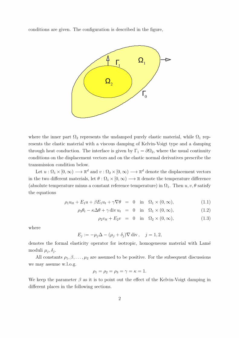
conditions are given. The configuration is described in the figure,

Ω1

Ω2

Γ0

Γ1

where the inner part Ω2 represents the undamped purely elastic material, while Ω1 rep-

resents the elastic material with a viscous damping of Kelvin-Voigt type and a damping

through heat conduction. The interface is given by Γ1 = ∂Ω2, where the usual continuity

conditions on the displacement vectors and on the elastic normal derivatives prescribe the

transmission condition below.

Let u : Ω1× [0,∞) −→ Rd and v : Ω2× [0,∞) −→ Rd denote the displacement vectors

in the two different materials, let θ : Ω1× [0,∞) −→ R denote the temperature difference

(absolute temperature minus a constant reference temperature) in Ω1. Then u, v, θ satisfy

the equations

ρ1utt + E1u+ βE1ut + γ∇θ = 0 in Ω1 × (0,∞), (1.1)

ρ3θt − κ∆θ + γ div ut = 0 in Ω1 × (0,∞), (1.2)

ρ2vtt + E2v = 0 in Ω2 × (0,∞), (1.3)

where

Ej := −µj∆− (µj + δj)∇ div , j = 1, 2,

denotes the formal elasticity operator for isotropic, homogeneous material with Lame

moduli µj, δj.

All constants ρ1, β, . . . , µ2 are assumed to be positive. For the subsequent discussions

we may assume w.l.o.g.

ρ1 = ρ2 = ρ3 = γ = κ = 1.

We keep the parameter β as it is to point out the effect of the Kelvin-Voigt damping in

different places in the following sections.

2

The transmission conditions on the interface Γ1 are given by

u = v on Γ1 × (0,∞), (1.4)

∂E1ν u+ θ ν + β∂E1

ν ut = ∂E2ν v on Γ1 × (0,∞), (1.5)

where

∂Ejν = −µj∂ν − (µj + δj)ν div ,

and

∂ν = ν∇

(in each of the n components if it is applied to a vector) with the normal vector ν at the

boundary as indicated in the picture above.

As remaining conditions on the smooth boundary we have

u = 0, θ = 0 on Γ0 × (0,∞), (1.6)

∂νθ = 0 on Γ1 × (0,∞). (1.7)

The initial-boundary transmission problem is completed by initial conditions,

u(·, 0) = u0, ut(·, 0) = u1, θ(·, 0) = θ0 in Ω1, (1.8)

v(·, 0) = v0, vt(·, 0) = v1 in Ω2. (1.9)

We are interested in the asymptotic behavior of solutions. If there is just the dissipative

problem in Ω1 (Ω2 = ∅), then the Kelvin-Voigt damping is sufficient to exponentially

stabilize the system. Therefore, it is interesting to see that even with an additional

damping given by heat conduction, the transmission problem no longer shows exponential

stability as we shall prove.

To prove the lack of exponential stability – often and in particular in one dimension

–, one can use the well-known criterion for contraction semigroups, which states that

the semigroup is exponentially stable if and only if the imaginary axis belongs to the

resolvent set and the resolvent operator is uniformly bounded on the imaginary axis.

Usually the non-uniform boundedness of the resolvent operator is shown by giving an

explicit sequence of exact solutions of the system. For higher dimensions this is often

not applicable due to the complexity of the resolvent operator. Here we compare the

system with an undamped reference system and then demonstrate that the difference of

the systems is of compact nature, and then apply Weyl’s theorem on the perturbation of

essential spectra by compact operators.

On the other hand, strong stability will be shown using the principle of unique con-

tinuation for the elastic operator in the isotropic case. That is, the damping material

stabilizes through the interface the whole systems, oscillations will be damped to zero.

3

Moreover, we can prove a polynomial decay using an extended version of the char-

acterization by Borichev and Tomilov [4], based on results of Latushkin and Shvydkov

[10].

The special character of the generators appearing with Kelvin-Voigt damping is un-

derlined by showing examples with non-compact inverses which is in contrast to standard

situations.

Our considerations immediately extend to the system without temperature,

ρ1utt + E1u+ βE1ut = 0 in Ω1 × (0,∞), (1.10)

ρ2vtt + E2v = 0 in Ω2 × (0,∞), (1.11)

with transmission conditions

u = v on Γ1 × (0,∞), (1.12)

∂E1ν u+ β∂E1

ν ut = ∂E2ν v on Γ1 × (0,∞), (1.13)

remaining boundary conditions

u = 0 on Γ0 × (0,∞), (1.14)

and initial conditions

u(·, 0) = u0, ut(·, 0) = u1 in Ω1, (1.15)

v(·, 0) = v0, vt(·, 0) = v1 in Ω2. (1.16)

Moreover, we may consider instead of the elastic operator the scalar Laplacian looking at

the corresponding transmission problem for wave equations for the scalar functions u, v,

ρ1utt − κ1∆u+ βκ1∆ut = 0 in Ω1 × (0,∞), (1.17)

ρ2vtt − κ2∆v = 0 in Ω2 × (0,∞), (1.18)

with positive constants κ1, κ2, and with transmission conditions

u = v on Γ1 × (0,∞), (1.19)

κ1∂νu+ βκ1∂νut = κ2∂νv on Γ1 × (0,∞), (1.20)

remaining boundary conditions

u = 0 on Γ0 × (0,∞), (1.21)


u(·, 0) = u0, ut(·, 0) = u1 in Ω1, (1.22)

v(·, 0) = v0, vt(·, 0) = v1 in Ω2. (1.23)

4

For wave equations with localized frictional damping it is well-known that the system is

exponentially stable when the damping is effective in a sufficient large neighborhood of

the boundary, see for example [8, 12, 14, 15]. For the one-dimensional Euler-Bernoulli

beam, also localized Kelvin-Voigt damping leads to exponential stability, as was shown by

K. Liu and Z. Liu in [11].

On the other hand, as was proved in one dimension in [11], Kelvin-Voigt damping is

not strong enough for the wave equation to give exponential stability in the transmission

problem. Here we now prove this for n ≥ 2.

The problem is related to the optimal design of material components, e.g. in damping

mechanisms for bridges or in automotive industry, see [3, 16] or [13] and the references

therein. As a consequence, one should consider various components with frictional damp-

ing if exponential stability is needed, for strong stability, where the oscillations at least

tend to zero as time tends to infinity, adding material with Kelvin-Voigt damping prop-

erties (plus or without heat) is sufficient.

The paper is organized as follows. In Section 2 we shortly discuss the well-posedness

of the thermo-viscoelastic transmission problem. In Section 3 we investigate smoothing

properties of the related purely thermo-viscoelastic system. The main Section 4 provideds

the proof of the lack of exponential stability. In Section 5, we prove the strong stability.

The polynomial stability will be given in Section 6. Section 7 provides examples for

Kelvin-Voigt operators yielding arguments for the non-compactness of the inverse of the

generator of the arising semigropus. In Section 8 the results on the related purely elastic

system and on problem for wave equations are given.

2 Well-posedness

Defining W := (u, v, ut, vt, θ)′ ( ′ meaning transpose), we formally get from (1.1)–(1.3) the

evolution equation

Wt(·, t) = AW (·, t)

with the (yet formal) operator A acting on Φ = (u, v, U, V, θ))′ as

AΦ =

U

V

−E1u− βE1U −∇θ−E2v

∆θ − divU

.

Introducing the spaces

H1 := (u, v) ∈ (H1(Ω1))d × (H1(Ω2))

d | u = 0 on Γ0, u = v on Γ1,

5

L2 := (L2(Ω1))d × (L2(Ω1))

d × L2(Ω2),

with the classical Sobolev spaces H1(. . . ), L2(. . . ), we choose as Hilbert space

H := H1 × L2,

with inner product

⟨Φ1,Φ2⟩H :=

∫Ω1

U1U2 + µ1∇u1∇u2 + (µ1 + δ1) div u1 div u2 + θ1θ2 dx+∫Ω2

V1V2 + µ2∇v1∇v2 + (µ2 + δ2) div v1 div v2 dx, (2.1)

where Φj = (uj, vj, Uj, Vj, θj)′.

The operator A is now defined as A : D(A) ⊂ H −→ H by

D(A) := Φ ∈ H | (U, V ) ∈ H1, (u+ βU, v) ∈ (H2(Ω1))d × (H2(Ω2))

d,

∂E1ν (u+ βU) + θ ν = ∂E2

ν v on Γ1 .

Then we have the dissipativity of the densely defined operator A,

Re ⟨AΦ,Φ⟩H = −β∫Ω1

µ1|∇U |2 + (µ1 + δ1)| divU |2 dx−∫Ω1

|∇θ|2 dx. (2.2)

The equality (2.2) and the choice of the inner product resp. of H reflects the energy

equality we have for (smooth) solutions of the transmission problem (1.1)–(1.9). That is,

if

E(t) ≡ E(u, θ, v ; t) :=1

2

(∫Ω1

|ut|2 + µ1|∇u|2 + (µ1 + δ1)| div u|2 + |θ|2 dx+∫Ω2

|vt|2 + µ2|∇v|2 + (µ2 + δ2)| div v|2 dx)

(2.3)

denotes the usual energy term associated to the equations, then

dE

dt(t) = −β

∫Ω1

µ1|∇ut|2 + (µ1 + δ1)| div ut|2 dx−∫Ω1

|∇θ|2 dx. (2.4)

Since the stationary transmission problem AΦ = F is uniquely solvable for any F ∈ H (cp.

[2, 9, 5]) with continuous inverse operator, we have that 0 ∈ ϱ(A) (resolvent set). Togetherwith the dissipativity (2.2), we conclude that A generates a contraction semigroup, hence

we have

Theorem 2.1. For any W 0 ∈ D(A) there exists a unique solution W to

Wt(t) = AW (t), W (0) = W 0,

satisfying

W ∈ C1([0,∞),H) ∩ C0([0,∞), D(A)).

6

3 Smoothing for pure thermo-viscoelasticity

Arguments needed to show the lack of exponential stability in Section 4 rely on the

smoothing effect in pure, uncoupled thermo-viscoelasticity as we shall prove it now. For

this purpose we consider the following thermo-viscoelastic initial value problem:

utt + E1u+ βE1ut +∇θ = 0 in Ω1 × (0,∞), (3.1)

θt −∆θ + div ut = 0 in Ω1 × (0,∞), (3.2)

with boundary conditions

u = 0, θ = 0 on (Γ0 ∪ Γ1)× (0,∞), (3.3)


u(·, 0) = u0, ut(·, 0) = u1, θ(·, 0) = θ0 in Ω1. (3.4)

Then we have the following version of a smoothing effect for t > 0:

Theorem 3.1. If

(u0, u1, θ0) ∈ (H10 (Ω1))

d × (L2(Ω1))d × L2(Ω1),

then the solution (u, θ) to (3.1)–(3.4) satisfies

(u, ut, utt) ∈ C0((0,∞), (H1

0 (Ω1))d × (H1

0 (Ω1))d × (H1(Ω1))

d),

(θ, θt, ) ∈ C0((0,∞), H2(Ω1)×H2(Ω1)

).

Proof: We present energy estimates for assumed smooth solutions which will prove

the theorem by density. Let

h(·, t) := t5u(·, t), p(·, t) := t5θ(·, t).

Then

htt + E1h+ βE1ht +∇p = 20t3u+ 10t4ut + 5βt4E1u, (3.5)

pt −∆p+ div ht = 5t4θ + 5t4 div ut. (3.6)

Multiplication of (3.5) by ht and (3.6) by p yields

dE1dt

(t) + β

∫Ω1

µ1|∇ht|2 + (µ1 + δ1)| div ht|2 dx+

∫Ω1

|∇p|2 dx =

∫Ω1

(20t3u+ 10t4ut + 5βt4E1u

)ht dx+

∫Ω1

(5t4θ + 5t4 div ut

)p dx, (3.7)

7

where

E1(t) := E(h, p ; t)

with

E(h, p ; t) := 1

2

(∫Ω1

|ht|2 + µ1|∇h|2 + (µ1 + δ1)| div h|2 + |p|2 dx).

Using

h(·, 0) = ht(·, 0) = p(·, 0) = 0,

we obtain, after integration with respect to t ∈ [0, T ], for some fixed T > 0,

2E1(t) +∫ t

0

(β

∫Ω1

µ1|∇ht|2 + (µ1 + δ1)| div ht|2 dx+

∫Ω1

|∇p|2 dx)

ds

≤ C

∫ t

0

∫Ω1

|ut|2 + |∇u|2 + |θ|2 dx ds, (3.8)

where C will denote a generic positive constant at most depending on T .

Differentiating in (3.5), (3.6) with respect to t, we have

httt + E1ht + βE1htt +∇pt = 60t2u+ 60t3ut + 10t4utt +

20βt3E1u+ 5βt4E1ut, (3.9)

ptt −∆pt + div htt = 20t3θ + 5t4θt + 20t3 div ut + 5t4 div utt. (3.10)

Similary as (3.8) we obtain

2E2(t) +∫ t

0

(β

∫Ω1

µ1|∇htt|2 + (µ1 + δ1)| div htt|2 dx+

∫Ω1

|∇pt|2 dx)

ds

≤ C

∫ t

0

∫Ω1

|utt|2 + |∇ut|2 + |∇u|2 + |θ|2 + |∇θ|2 dx ds, (3.11)

where

E2(t) := E(ht, pt ; t).

Continuing this way in differentiating the differential equations two more times, we get

similar estimates for the third- and fourth-order energy terms

E3(t) := E(htt, ptt ; t), E4(t) := E(httt, pttt ; t).

Since the first-order energy for (u, θ),

E1(t) := E(u, θ ; t),

8

satisfies

E1(t) + β

∫Ω1

µ1|∇ut|2 + (µ1 + δ1)| div ut|2 dx+

∫Ω1

|∇θ|2 dx = E1(0), (3.12)

we conclude, using the ellipticity of the operators E1 and ∆,∫Ω1

|ut|2 + |∇u|2 + |∇ht|2 +∇htt|2 + |∇httt|2 dx+ ∥(p, pt, ptt∥2H2 ≤

C

(E1(0) +

∫ t

0

∫Ω1

|∇(u, ut, utt)|2 + |(θ, θt, θtt)|2 + |∇(θ, θt, θtt)|2 dx ds

). (3.13)

Letting η > 0 be arbitrarily small, but fixed, we have from

∇ht = 5t4∇u+ t5∇ut

the estimate

|∇ut(·, t)|2 ≤C

η2(|∇ht(·, t)|2 + |∇u(·, t)|2

),

and so on. This way, we obtain, with a constant Cη depending at most on T and on η,

for t ≥ η,

f(t) := ∥(u, ut, utt, uttt)(·, t)∥2H1 + ∥(θ, θt, θtt)(·, t)∥2H2 ≤ Cδ

(E(0) +

∫ t

0

f(s) ds

).

By Gronwall, this implies

u ∈ W 3,2([η, T ], (H1(Ω1)

d), θ ∈ W 2,2

([η, T ], H2(Ω1)

).

By embedding, we complete the proof of Theorem 3.1.

4 Lack of exponential stability

The proof that the semigroup is not exponentially stable will use the so-called Weyl

theorem, saying that the essential spectrum of a bounded operator is invariant under

compact perturbations (see [7]). The basic idea is to consider, in addition to the given

semigroup S with (S(t) = etA)t≥0 describing our transmission problem above, another

semigroup S0 with (S0(t))t≥0, for which the essential type ωess(S0) is known to be zero,

e. g. for the unitary semigroup defined below, and then to show that the difference

S(t)− S0(t) is a compact operator (for some resp. all t > 0). This implies, using Weyl’s

theorem, that the essential types of S and of S0 are the same, hence we will have for the

type ω0(S) of the semigroup S that

ω0(S) ≥ ωess(S) = ωess(S0) = 0,

9

hence the semigroup S will not be exponentially stable.

Actually, the arguments will be more subtle, since we cannot argue with S and S0

directly, due to regularity properties, but we have to exploit the smoothing effect proved

in the previous section to argue in a modified setting, see the proof of Theorem 4.4 below.

We define the new semigroup S0 by the following initial boundary value problem over

Ω1 ∪ Ω2:

utt + E1u+ βE1ut +∇θ = 0 in Ω1 × (0,∞), (4.1)

θt −∆θ + div ut = 0 in Ω1 × (0,∞), (4.2)


u = 0, θ = 0 on (Γ0 ∪ Γ1)× (0,∞), (4.3)


u(·, 0) = u0, ut(·, 0) = u1, θ(·, 0) = θ0 in Ω1, (4.4)

as well as

vtt + E2v = 0 in Ω2 × (0,∞), (4.5)


v = 0 on Γ1 × (0,∞), (4.6)


v(·, 0) = v0, vt(·, 0) = v1 in Ω2. (4.7)

The problem in Ω1 is the purely thermo-viscoelastic problem studied in the previous

section. The problem in Ω2 is energy conserving, i. e.∫Ω2

|vt|2 + µ2|∇v|2 + (µ2 + δ2)| div v|2 dx =

∫Ω2

|v1|2 + µ2|∇v0|2 + (µ2 + δ2)| div v0|2 dx.

Hence, the contraction semigroup S0 associated to (4.1)–(4.7) has type

ω0(S0) = 0. (4.8)

Lemma 4.1. Let ((u0n, u

1n, θ

0n))n be a sequence of initial data which is bounded in

(H10 (Ω1))

d × (H10 (Ω1))

d ×H10 (Ω1),

and let ((un, θn))n denote the associated solutions to the purely thermo-viscoelastic problem

(4.1)–(4.4). Then there exists a subsequence, again denoted by ((un, θn))n, such that

un + βun,t → u+ βut strongly in L2((0, T ),

((H1(Ω1)

)d),

10

and

θn → θ strongly in L2((0, T ), H1(Ω1)

),

for some (u, θ).

Proof: Writing (mostly) in the proof for simplicity

u := un, θ := θn,

and multiplying the differential equations (4.1) and (4.2) by utt and θt, respectively, we

obtain, after integration,∫ t

0

∫Ω1

|utt|2 dx ds+1

2

∫Ω1

µ1∇u∇ut + (µ1 + δ1) div u div ut dx+

β

2

∫Ω1

µ1|∇ut|2 + (µ1 + δ1)| div ut|2 dx+Re

∫ t

0

∫Ω1

∇θ utt dx ds =

1

2

∫Ω1

µ1∇u0∇u1 + (µ1 + δ1) div u0 div u1 dx+

β

2

∫Ω1

µ1|∇u1|2 + (µ1 + δ1)| div u1|2 dx

+

∫ t

0

∫Ω1

µ1|∇ut|2 + (µ1 + δ1)| div ut|2 dx ds,

and∫ t

0

∫Ω1

|θt|2 dx ds+1

2

∫Ω1

|∇θ|2 dx =

∫Ω1

|∇θ0|2 dx− Re

∫ t

0

∫Ω1

div ut θt dx ds. (4.9)

Summing up, we obtain from the last two identities for t ∈ [0, T ], T > 0 arbitrary, but

fixed,∫ t

0

∫Ω1

|utt|2 dx ds+ β

∫Ω1

µ1|∇ut|2 + (µ1 + δ1)| div ut|2 dx+∫ t

0

∫Ω1

|θt|2 dx ds+

∫Ω1

|∇θ|2 dx ≤ C

∫Ω1

|∇u0|2 + |∇u1|2 + |u1|2 + |∇θ0|2 dx, (4.10)

where C a positive constant (at most depending on T ). Since

E1(u+ βut) = −utt −∇θ,

we conclude from (4.10) the boundedness of (un + βun,t)n in L2((0, T ), ((H2(Ω1))

d).

Moreover, we conclude the boundedness of (un,t + βun,tt)n in L2((0, T ), (L2(Ω1))

d).

By Aubin’s compactness theorem, we obtain that there exists a subsequence with


(H1(Ω1)

)d), (4.11)

11

for some u ∈ L2((0, T ), (H1(Ω1))

d). Finally, we get from (4.10) and (4.2) that (θn)n is

bounded in L2 ((0, T ), H2(Ω1)) and that (θn,t)n is bounded in L2 ((0, T ), L2(Ω1)), which

implies by Aubin’s theorem that there is subsequence such that

θn → θ strongly in L2((0, T ), H1(Ω1)

), (4.12)

for some θ ∈ L2 ((0, T ), H1(Ω1)). This completes the proof of Lemma 4.1.

Remark 4.2. The convergence in (4.11) and (4.12), respectively, can be obtained, for

any ε > 0, in the space

L2((0, T ),

(H2−ε(Ω1)

)d)and

L2((0, T ), H2−ε(Ω1)

),

respectively.

Lemma 4.3. Let w be the solution (with sufficient regularity for the following integrals

to exist) to

wtt + E2w = f in Ω2 × (0, T ),

with boundary condition

w = 0 on Γ1 × (0, T ),

where T > 0 is arbitrary, but fixed. Then w satisfies∫ T

0

∫Γ1

|∂νw|2 + | divw|2 do ds ≤ CT

(∫ T

0

∫Ω2

|wt|2 + |∇w|2 + |f |2 dx ds +∫Ω2

|wt(·, 0)|2 + |∇w(·, 0)|2 dx),

for some constant CT > 0 depending at most on T .

Lemma 4.3 easily follows by multiplication of the differential equation with q∇w in

(L2(Ω1))d, where q is a smooth vector field satisfying q = ν on Γ1, cp. [6, Lemma 4.1]

and the proof Lemma 6.3 below. Now we state the main theorem:

Theorem 4.4. The semigroup S with S(t) = eAt is not exponentially stable.

Proof: Having an application of Weyl’s theorem in mind, we prove a compactness

result. For this purpose, let ((u0n, v

0n, u

1n, v

1n, θ

0n))n be a bounded sequence of initial data in

the space

H0 :=(H1

0 (Ω1))d × (H1

0 (Ω2))d × (L2(Ω1)

)d × (L2(Ω2))d ×H1

0 (Ω1).

12

Let (un, vn, θn) be the corresponding solution to the transmission problem (1.1)–(1.9)

– with associated semigroup S(t) = eAt –, and let (un, vn, θn) be the solution to the

uncoupled problem (4.1)–(4.7) – with associated semigroup S0(t) ≡ eAt. Let the difference,

for which we wish to show convergence inH for some subsequence, be defined as (dropping

n in some places)

w := un − un, z := vn − vn, η := θn − θn.

Then (w, z, η) satisfies the differential equations

wtt + E1w + βE1wt +∇η = 0 in Ω1 × (0,∞), (4.13)

ηt −∆η + divwt = 0 in Ω1 × (0,∞), (4.14)

ztt + E2z = 0 in Ω2 × (0,∞), (4.15)

with zero initial data,

w(·, 0) = 0, wt(·, 0) = 0, η(·, 0) = 0 in Ω1, (4.16)

z(·, 0) = 0, zt(·, 0) = 0 in Ω2. (4.17)

Moreover, the following boundary conditions are in particular satisfied:

w = 0, η = 0 on Γ0 × (0,∞), (4.18)

w = u, η = θ on Γ1 × (0,∞), (4.19)

z = v on Γ1 × (0,∞). (4.20)

As usual, we obtain for the associated energy (indicating the dependence on n), cp. (2.3),

E(w, z, η ; t) =1

2

(∫Ω1

|wt|2 + µ1|∇w|2 + (µ1 + δ1)| divw|2 + |η|2 dx+∫Ω2

|zt|2 + µ2|∇z|2 + (µ2 + δ2)| div z|2 dx)

=: En(t), (4.21)

the identity

d

dtEn(t) + β

∫Ω1

|∇wt|2 + |∇η|2 dx =

∫Γ1

(−∂E1

ν w − β∂νwt + ν η)wt do

+

∫Γ1

∂νη η do+

∫Γ1

∂E2ν z zt do. (4.22)

This implies, using the boundary conditions (4.18)–(4.20) and the transmission conditions

(1.4), (1.5),

En(t) ≤∫ t

0

∫Γ1

(∂E1ν (un + βun,t)

)un,t do ds−

∫ t

0

∫Γ1

∂E2ν vn un,t do ds

+

∫ t

0

∫Γ1

∂ν θn θn do ds ≡ J1n + J2

n + J3n. (4.23)

13

Since we get the same for differences un−um, · · · , and since the energy term is equivalent

to the norm in the underlying Hilbert space H, it suffices to show that En converges.

Using Lemma 4.1, see also Remark 4.2, we know


(H1(Ω1)

)d),

implying

∂E1ν (un + βun,t)→ ∂E1

ν (u+ βut) strongly in L2

((0, T ),

(H− 1

2 (Γ1))d)

.

Since also

un,t → ut strongly in L2

((0, T ),

(H

12 (Γ1)

)d),

we get the convergence of (J1n)n. By Lemma 4.3 and using the differential equation (4.5),

we obtain the weak convergence

∂E2ν vn ∂E2

ν v weakly in L2((0, T ),

(L2(Γ1)

)d),

and with the boundedness of (un,t)n in L2((0, T ), ((L2(Γ1))

d), we conclude the conver-

gence of (J2n)n. The convergence of (J3

n)n follows from Lemma 4.1 resp. Remark 4.2,

because

∂ν θn → ∂ν θ strongly in L2((0, T ), H− 1

2 (Γ1)),

and

θn → θ strongly in L2((0, T ), H

12 (Γ1)

).

Hence we have proved that a bounded sequence of initial data (Φn)n in H0 leads to a

convergent subsequence of ((S(t)− S0(t))Φn)n in H, for any t > 0, a property which we

call compactness over H0.

Let

H0 :=(H1

0 (Ω1))d × (L2(Ω2)

)d × (L2(Ω1))d × (L2(Ω2)

)d × L2(Ω1).

Then, fixing δ > 0, we have

S0(δ)H0 ⊂ H0,

because of the smoothing property proved in Section 3. We consider

H := S(r)S0(δ)Φ0 |Φ0 ∈ H0, r ≥ 0,

with closure in H, allowing us to exploit the smoothing property. H is an invariant

subspace for the semigroup S, with H0 being a closed subset of H. If P denotes the

orthogonal projection onto H0, then, for fixed t > 0,

S(t)− S0(t)S0(δ)P : H −→ H

14

is compact by the compactness overH0 as proved above, since S0(δ)H0 is a dense subspace

of H. Therefore, we can apply Weyl’s theorem on compact perturbations of the essential

spectrum. Since in Hωess(S0S(δ)P ) = 0,

we thus get there

ωess(S) = 0,

implying that S is not exponentially stable also in H. This completes the proof of Theo-

rem 4.4.

5 Strong stability

Though not exponentially stable, the damping thermo-viscoelastic part in Ω1 is damping

for the whole system in the sense of strong stability. For the proof we use in particular the

principle of unique continuation for the elastic operator for homogeneous isotropic media.

Theorem 5.1. (1) iR ⊂ ϱ(A).(2) The semigroup

(etA)t≥0

is strongly stable, i.e. we have for any W 0 ∈ H:

etAW 0 → 0, as t→∞.

Proof. (2) is a direct consequence of (1), hence it suffices to prove prove (1).

Remark 5.2. Since A−1 is not expected to be compact – compare the discussion of Kelvin-

Voigt operators in Section 7 –, it is not sufficient to just exclude imaginary eigenvalues

of A.

Since 0 ∈ ϱ(A), there is R1 > 0 such that i[−R1, R1] ⊂ ϱ(A). Let

∞ ≥ λ∗ := supN,

where

N := R > 0 | i[−R,R] ⊂ ϱ(A) .

Then λ∗ > 0, since R1 ∈ N . If λ∗ =∞ the proof is complete. So assume

0 < λ∗ <∞.

Then there exists a sequence (λn)n ⊂ R such that

limn→∞

∥(iλn −A)−1∥ =∞.

15

This implies the existence of (Fn)n ⊂ H with

∥Fn∥ = 1, limn→∞

∥(iλn −A)−1Fn∥ =∞.

Denoting Φn := (iλn −A)−1Fn and Φn := Φn/∥Φn∥, as well as Fn := Fn/∥Φn∥, we have

(iλn −A)Φn = Fn

and

∥Φn∥ = 1, Fn → 0 strongly in H.

By the dissipativity (2.2) we then obtain

β

∫Ω1

µ1|∇Un|2 + (µ1 + δ1)| divUn|2 dx+

∫Ω1

|∇θn|2 dx = −Re ⟨AΦn,Φn⟩H

= −Re ⟨Fn,Φn⟩H → 0,

hence

Un → 0 strongly in(H1(Ω1)

)d, θn → 0 strongly in H1(Ω1).

Denoting Fn = (Fn,1, . . . , Fn,5)′, and since

iλnun − UnF1,n,

we have

un → 0 strongly in(H1(Ω1)

)d.

By the boundedness of ∥Φn∥H we conclude that there exist subsequences such that

vn → v strongly in(L2(Ω1)

)d,

and

vn → v weakly in(H1(Ω1)

)d.

Moreover,

iλnVn − µ2∆vn − (µ2 + δ2)∇ div vn = F4,n,

implying∫Ω2

µ2|∇vn|2 + (µ2 + δ2)| div vn|2 dx =

∫Γ1

∂E2ν vnvn do− iλn

∫Ω2

Vnvn dx+∫Ω2

F4,nvn dx.

Since

∂E1ν un + θ ν + β∂E1

ν Un = ∂E2ν vn,

16

we conclude that

∂E2ν vn → 0 strongly in

(H− 1

2 (Γ1))d

.

With the boundedness of (vn)n in(H

12 (Γ1)

)d, we have∫

Γ1

∂E2ν vnvn do→ 0.

Thus, we conclude the strong convergence of (vn)n in (H1(Ω2))d. Hence, Φn converges

strongly to some Φ ∈ H with ∥Φ∥H = 1. Since AΦn = iλnΦn−Fn now converges strongly

to iλϕ (with λ = ±λ∗), we obtain

Φ ∈ D(A), (iλ−A)Φ = 0.

We successively conclude, using the dissipativity once more, θ = 0, U = 0, u = 0, v|Γ1 = 0,

∂E2ν v|Γ1 = 0, and

iλv − V = 0,

iλV + E2v = 0.

Hence we have for v

E2v = λ2v, (5.1)

v|Γ1 = 0, ∂E2ν v|Γ1 = 0. (5.2)

By the unique continuation principle for solutions to (5.1), (5.2), i. e. for isotropic,

homogeneous elasticity (see [18, 1, 17]), we get

v = 0.

Hence Φ = 0 which is a contradiction to ∥Φ∥H = 1. This completes the proof of Theo-

rem 5.1.

6 Polynomial stability

In addition to the strong stability, we shall prove the following polynomial decay result.

Theorem 6.1. The semigroup(etA)t≥0

decays polynomially of order at least 13, i.e.

∃C > 0 ∃ t0 > 0 ∀ t ≥ t0 ∀Φ0 ∈ D(A) : ∥etAΦ0∥H ≤ C t−13∥AΦ0∥H. (6.1)

For the proof we shall use the following extension of a result of Borichev and Tomilov

[4] resp. Latushkin and Shvydkoy [10] for a general contraction semigroup (T (t))t≥0 =(etB)t≥0

in a Hilbert space H1 with iR ⊂ ρ(B).

17

Lemma 6.2. Let (T (t))t≥0 =(etB)t≥0

be a contraction semigroup in a Hilbert space H1

with iR ⊂ ρ(B). Then the following characterizations (6.2) and (6.3) are equivalent, where

the parameters α, β ≥ 0 are fixed:

∃C > 0 ∃λ0 > 0 ∀λ ∈ R, |λ| ≥ λ0 ∀F ∈ D(Bα) : ∥ (iλ− B)−1 F∥H ≤ C|λ|β∥BαF∥H,(6.2)

∃C > 0 ∃ t0 > 0 ∀ t ≥ t0 ∀Φ0 ∈ D(B) : ∥etBΦ0∥H ≤ C t−1

α+β ∥BΦ0∥H. (6.3)

Proof of Lemma 6.2: For α = 0 it is part of the results in [4, Theorem 2.4]. To

extend the proof there to the case α > 0, one has to extend [10, Theorem 3.2] which is

possible due to the following observation: [10, Theorem 3.2] proves the equivalence of

supλ

∥ (λ− B)−1 ∥

1 + |λ|α

<∞ and sup

λ

∥ (λ− B)−1 B−α∥

<∞ (6.4)

for λ in a strip a < Reλ < b. In the proof there, it is shown that

d1∥ (λ− B)−1 x∥

|λ|α−Kα∥x∥ ≤ ∥ (λ− B)−1 B−αx∥ ≤ d2

∥ (λ− B)−1 x∥|λ|α

+Kα∥x∥ (6.5)

holds for x ∈ H1, with positive constants d1, d2, Kα. But this immediately implies

d1∥ (λ− B)−1 x∥1 + |λ|α+β

−Kα∥x∥

1 + |λ|β≤ ∥ (λ− B)−1 B−αx∥

1 + |λ|β

≤ d2∥ (λ− B)−1 x∥1 + |λ|α+β

+Kα∥x∥

1 + |λ|β(6.6)

with positive constants d1, d2. Hence we have the equivalence of

supλ

∥ (λ− B)−1 ∥1 + |λ|α+β

<∞ and sup

λ

∥ (λ− B)−1 B−α∥

1 + |λ|β

<∞, (6.7)

and [10, Theorem 3.2] is thus extended. Then one can use the results in [4], and this

proves Lemma 6.2.

In the sequel we will prove (6.2) for α = 1 and β = 2 which will then prove Theorem 6.1

by Lemma 6.2. For the proof we need the following Lemma, in particular in order to

estimate tangential derivatives on Γ1, since qν will there be positive.

Lemma 6.3. Let x0 ∈ Ω2 and q(x) := x− x0 for x ∈ Ω2. Let w,W and λ ∈ R satisfy

iλw −W = g2 ∈(L2(Ω2)

)d, (6.8)

iλW + E2w = g4 ∈(L2(Ω2)

)d. (6.9)

18

Then we have

1

2

∫Ω2

|λw|2 + µ2|∇w|2 + (µ2 + δ2)| divw|2 dx+µ2

2

∫Γ1

(qν)|∇τw|2 do

−1

2

∫Γ1

(qν)(|λw|2 + µ2|∂νw|2 + (µ2 + δ2)| divw|2

)do

−µ2Re

∫Γ1

∂νwjq∇τwj do+ (µ2 + δ2)Re

∫Γ1

(qν) divw((∇τwj)/j − νjqk(∇τwj)/k

)do

−µ2d− 1

2Re

∫Γ1

∂νww do− (µ2 + δ2)d− 1

2Re

∫Γ1

(∇τwj)/jνkwk + (∂νwj)/jνkwk do

= Re

∫Ω2

(iλg2 + g4)(qk∂kw + w) dx, (6.10)

where ∇τ denotes tangential derivatives.

Proof: We obtain from (6.8), (6.9)

−λ2w + E2w = iλg2 + g4. (6.11)

Multiplying this by qk∂kw in (L2(Ω2))nand performing a partial integration, we get

Re

∫Ω2

(iλg2 + g4)qk∂kw dx = −1

2

∫Γ1

(qν)|λw|2 do+ d

2

∫Ω2

|λw|2 dx︸︷︷︸=:I1

−µ2Re

∫Γ1

ν∇wjqk∂kwj do+ µ2Re

∫Ω2

∇wj∇(qk∂kwj) dx

−(µ2 + δ2)Re

∫Γ1

divwνjqk∂kwj do+ (µ2 + δ2)Re

∫Ω2

divw div (qk∂kw) dx

≡ I1 + I2 + I3 + I4 + I5. (6.12)

Observing

∇wj = ∇τwj + ⟨∇wj, ν⟩Cnν, div q = d,

we obtain

I2 = −µ2

∫Γ1

(qν)|∂νw|2 do− µ2Re

∫Γ1

∂νwj q∇τwj do, (6.13)

I3 = µ2

(1− d

2

)∫Ω2

|∇w|2 dx+µ2

2

∫Γ1

(qν)|∇τw|2 do+µ2

2

∫Γ1

(qν)|∂νw|2 do, (6.14)

I4 = −(µ2 + δ2)

∫Γ1

(qν)| divw|2 dx+

(µ2 + δ2)Re

∫Γ1


)do, (6.15)

I5 = (µ2 + δ2)

(1− d

2

)∫Ω2

| divw|2 dx+(µ2 + δ2)

2

∫Γ1

(qν)| divw|2 do. (6.16)

19

Summarizing (6.12)–(6.16) we conclude

−1

2

∫Γ1

(qν)(|λw|2 + µ2|∂νw|2 + (µ2 + δ2)| divw|2

)do+

d

2

∫Ω2

|λw|2 dx+

µ2

(1− d

2

)∫Ω2

|∇w|2 dx+µ2

2

∫Γ1

(qν)|∂νw|2 do+

(µ2 + δ2)

(1− d

2

)∫Ω2

| divw|2 dx− µ2Re

∫Γ1

∂νwj q∇τwj do+

(µ2 + δ2)Re

∫Γ1


)do

= Re

∫Ω2

(iλg2 + g4)qk∂kw dx. (6.17)

Multiplying (6.11) by η w for some η > 0, we obtain

−η∫Ω2

|λw|2 dx+ ηµ2

∫Ω2

|∇w|2 dx+ η(µ2 + δ2)

∫Ω2

| divw|2 dx

−ηµ2

∫Γ1

∂νww do− η(µ2 + δ2)

∫Γ1

(∇τwj)/jνkwk do

−η(µ2 + δ2)

∫Γ1

(∂νwj)/jνkwk do = ηRe

∫Ω2

(iλg2 + g4)w dx. (6.18)

Choosing η := d−12

and then adding (6.17) and (6.18), we obtain the claim of Lemma 6.3.

Now, we can present the Proof of Theorem 6.1 in proving (6.2) for α = 1 and β = 2.

Let λ ∈ R (sufficiently large in case), (iλ−A) Φ = F = (f1, f2, f3, f4, f5)′ ∈ D(A).

Then, denoting again Φ = (u, v, U, V, θ)′, we have

iλu− U = f1, (6.19)

iλv − V = f2, (6.20)

iλU + E1u+ βE1U +∇θ = f3, (6.21)

iλV + E2v = f4, (6.22)

iλθ −∆θ + divU = f5. (6.23)

We obtain from the dissipativity (2.2)∫Ω1

µ1|∇U |2 + (µ1 + δ1)| divU |2 dx+

∫Ω1

|∇θ|2 dx ≤ ∥F∥H∥Φ∥H. (6.24)

This implies ∫Ω1

|U |2 + |θ|2 dx ≤ C∥F∥H∥Φ∥H, (6.25)

20

where the letter C will be used in the sequel to denote positive constants not depending

on λ, ϕ or F . Using (6.19) and (6.25) we obtain∫Ω1

|u|2 + |∇u|2 dx ≤ C(∥F∥H∥Φ∥H + ∥F∥2H

). (6.26)

It remains to estimate∫Ω2|∇v|2 + |V |2 dx appropriately, which is the difficult part and

where we need in particular powers of |λ| on the right-hand sides as well as the property

of F to belong to the domain of A.Let

z := u+ βU, ϑ := (1 + iλβ)v.

Then we get from (6.21)–(6.23)

(1 + iλβ)E1z = −(1 + iλβ)∇θ − (1 + iλβ)iλU + (1 + iλβ)f3,

E2ϑ = −(1 + ıλβ)iλV + (1 + iλβ)f4,

−∆θ = −iλ divU − iλθ + f5,

with transmission conditions on Γ1,

z = ϑ− βf2, (1 + iλβ)∂E1ν (z + θ ν) = ∂E2

ν ϑ,

and boundary conditions z = 0, θ = 0 on Γ0, and ∂νθ = 0 on Γ1. By elliptic regularity

theory we obtain, assuming λ ≥ 1 w.l.o.g.,

|1 + iλβ|∥z∥H2(Ω1) + ∥ϑ∥H2(Ω2) + ∥θ∥H2(Ω1) ≤C|λ|2

(∥U∥L2(Ω1) + ∥ divU∥L2(Ω1

+ ∥V ∥L2(Ω2) + ∥θ∥L2(Ω1)

)+C|λ|∥F∥H + C∥f2∥H2(Ω2) ≤

C(|λ|2∥V ∥L2(Ω2) + |λ|2∥F∥

12H∥Φ∥

12H + |λ|∥AF∥H

), (6.27)

where we used (6.24) and

∥f2∥H 32 (Γ1)

≤ C∥f2∥H2(Ω2) ≤ C∥AF∥H. (6.28)

By interpolation we obtain, using (6.24)–(6.26),

∥z∥H3/2(Ω1) + ∥∇z∥L2(Γ1) ≤ C∥z∥12

H1(Ω1)∥z∥

12

H2(Ω1)

≤ C

|1 + iλβ| 12

(∥F∥

14H∥Φ∥

14H + ∥F∥

12H

)(|λ|∥V ∥

12

L2(Ω2)+ |λ|∥F∥

14H∥Φ∥

14H + |λ|

12∥AF∥

12H

)≤ C|λ|

12

(∥AF∥

14H∥Φ∥

14H∥V ∥

12

L2(Ω2)+ ∥AF∥

12H∥Φ∥

12H + ∥AF∥

34H∥Φ∥

14H+

∥AF∥12H∥V ∥

12

L2(Ω2)+ ∥AF∥

34H∥Φ∥

14H + ∥AF∥H

)≤ C|λ|

12

((∥AF∥

14H∥Φ∥

14H + ∥AF∥

12H

)∥V ∥

12

L2(Ω2)+ ∥AF∥

12H∥Φ∥

12H+

∥AF∥34H∥Φ∥

14H + ∥AF∥H

). (6.29)

21

In order to estimate∫Ω2|∇v|2 + |V |2 dx we apply Lemma 6.3 for w := v, W := V2 with

g2 := f2, g4 := f4. Using the strict positivity of qν on Γ1, we obtain

∥V ∥2L2(Ω2)+ ∥∇v∥2L2(Ω2)

+ ∥∇τv∥2L2(Γ1)≤

C(∥v∥2L2(Γ1)

+ ϵ∥∇τv∥2L2(Γ1)+ Cϵ

(∥∂νv∥2L2(Γ1)

+ ∥ div v∥2L2(Γ1)

)+|λ|2

(∥f2∥2L2(Ω2)

+ ∥f4∥2L2(Ω2)

)+ ∥f2∥2L2(Ω2)

), (6.30)

where Cϵ > 0 depends on ϵ, and ε is chosen small enough to get rid of the term ϵ∥∇τv∥2L2(Γ1)

on the right-hand side of (6.30). The last term in (6.30) arises from the estimate

∥V ∥2L2(Ω2)≤ 2∥λv∥2L2(Ω2)

+ 2∥f2∥2L2(Ω2).

To further estimate this term we need the following type of Poincare inequality.

Lemma 6.4.

∃K > 0 ∀F ∈ H : ∥f2∥L2(Ω2) ≤ K(∥∇f2∥L2(Ω2) + ∥∇f1∥L2(Ω1).

)Proof: Assuming that the inequality does not hold we get a sequence (Fn)n in H

with Fn = (f1,n, f2,n, f3,n, f4,n, f5,n)′ such that

∥∇f2,n∥L2(Ω2) + ∥∇f1,n∥L2(Ω1) ≤1

n∥f2,n∥L2(Ω2).

Defining

gn :=f1,n

∥f2,n∥L2(Ω2)

, hn :=f2,n

∥f2,n∥L2(Ω2)

,

we conclude, using gn = 0 on Γ0, that gn → g := 0 in H1(Ω1) as well as (gn)|Γ1 → g|Γ1 = 0

in L2(Γ1). Since ∇hn → 0 in L2(Ω2), and ∥hn∥L2(Ω2) = 1 we obtain from Rellich’s

compactness theorem that hn → h in H1(Ω2) and hn → h in L2(Γ1) for some h satisfying

∇h = 0. This implies h = k for some constant k.

On the other hand we know gn = hn on Γ1 (reflecting the transmission condition in

H) which implies h = g = 0 on Γ1 and hence k = 0, giving h = 0 in Ω2. This is a

contradiction to ∥h∥L2(Ω) = limn ∥hn∥L2(Ω) = 1 and hence proves the Lemma.

With this Lemma we conclude from (6.30)

∥V ∥2L2(Ω2)+ ∥∇v∥2L2(Ω2)

≤ C(∥AF∥H∥Φ∥H + ∥AF∥2H+

∥∂νv∥2L2(Γ1)+ ∥ div v∥2L2(Γ1)

+ |λ|2∥AF∥2H). (6.31)

The following series of estimates now concerns the term ∥∂νv∥2L2(Γ1)+ ∥ div v∥2L2(Γ1)

where

the transmission conditions will be exploited again. We observe

(1 + iλβ)∂νv = ∂νϑ, (1 + iλβ) div v = div ϑ.

22

Hence, with c1 := 2µ2(µ2 + δ2),

C|1 + iλβ|2(∥∂νv∥2L2(Γ1)

+ ∥ div v∥2L2(Γ1)

)≤ |µ2|2∥∂νϑ∥2L2(Γ1)

+ |µ2 + δ2|2∥ div ϑ∥2L2(Γ1)

= ∥∂E2ν ϑ∥2L2(Γ1)

− c1

∫Γ1

∂νϑ div ϑ ν do

= ∥∂E2ν ϑ∥2L2(Γ1)

− c1

∫Γ1

∂νϑ div (ϑ− (z + f2)) ν do

−c1∫Γ1

∂νϑ div (z + f2) ν do

≡ (|1 + iλβ|2)(I + II + III). (6.32)

Observing

(1 + iλβ)∂E1ν (z + θ ν) = ∂E2

ν ϑ

we have

I ≤ 2∥∂E1ν z∥2L2(Γ1)

+ 2∥θ∥2L2(Γ1)

≤ 2∥z∥2H3/2(Ω1)+ C∥AF∥H∥Φ∥H.

by (6.24). Next, using (6.28),

|III| ≤ ε∥∂νϑ∥2L2(Γ1)+ Cε

(∥z∥2H3/2(Ω1)

+ ∥f2∥2H1(Γ1)

)≤ ε∥∂νϑ∥2L2(Γ1)

+ Cε

(∥z∥2H3/2(Ω1)

+ ∥AF∥2H). (6.33)

Using ϑ = z + βf2 on Γ1, we have

div (ϑ− (z + f2)) = ν ∂ν (ϑ− (z + f2)) .

This implies

II = −c1∥∂νϑ∥2L2(Γ1)+ c1

∫Γ1

(∂νϑ ν)(∂ν z + ∂ν f2

)ν do

≡ −c1∥∂νϑ∥2L2(Γ1)+ II.

Since we may neglect the negative term −c1∥∂νϑ∥2L2(Γ1)later on, and since

|II| ≤ ε∥∂νϑ∥2L2(Γ1)+ Cε

(∥∂νz∥2L2(Γ1)

+ ∥∂νf2∥2L2(Γ1)

)≤ ε∥∂νϑ∥2L2(Γ1)

+ Cε

(∥z∥2H3/2(Ω1)

+ ∥AF∥2H), (6.34)

we get from (6.32)–(6.34), choosing ε small enough,

∥∂νv∥2L2(Γ1)+ ∥ div v∥2L2(Γ1)

≤ C(∥z∥2H3/2(Ω1)

+ ∥AF∥2H + ∥AF∥H∥Φ∥H). (6.35)

23

Combining (6.29) and (6.35) we obtain

∥∂νv∥2L2(Γ1)+ ∥ div v∥2L2(Γ1)

≤ C|λ|((∥AF∥

12H∥Φ∥

12H + ∥AF∥H

)∥V ∥L2(Ω2)+

∥AF∥H∥Φ∥H + ∥AF∥32H∥Φ∥

12H + ∥AF∥2H

)≤ c|λ|2

(∥AF∥H∥Φ∥H + ∥AF∥

32H∥Φ∥

12H

+∥AF∥2H)+

1

2∥V ∥2L2(Ω2)

. (6.36)

A combination of (6.31) and (6.36) yields

∥V ∥2L2(Ω2)+ ∥∇v∥2L2(Ω2)

≤ C|λ|2(∥AF∥H∥Φ∥H + ∥AF∥2H + ∥AF∥

32H∥Φ∥

12H

). (6.37)

Finally combining (6.24)–(6.26) and (6.37) we have proved the estimate

∥Φ∥2H ≤ C|λ|4∥AF∥2H +1

2∥Φ∥2H

implying

∥ (iλ−A)−1 F∥H ≤ C|λ|2∥AF∥H

which completes the proof of Theorem 6.1.

7 On the lack of compactness of the inverse

We present examples to underline that the compactness of the inverse A−1 cannot be

expected (cp. Remark 5.2).

7.1 Wave equation or Kirchhoff plate equation

We look at the classical Kelvin-Voigt damping – without transmission, Ω2 = ∅ – for the

wave equation or the Kirchhoff plate equation, respectively, i.e. for

vtt −∆(v + βvt) = 0, v = 0 on Γ, (7.1)

or

vtt +∆2(v + βvt) = 0, v = ∆v = 0 on Γ, (7.2)

where

Γ := Γ0 ∪ Γ1 = ∂Ω1.

If A denotes either −∆ or ∆2 (with corresponding boundary conditions in its domain),

then the usual transformation to a first-order system yields the stationary operator

B

(f

g

)=

(g

−A(f + βg)

).

24

We look at the eigenvalue problem

B

(f

g

)= λ

(f

g

).

This turns into the equation

−(1 + βλ)Af = λ2f.

Let

λ0 := −1

β.

For λ = λ0 we conclude f = g = 0, hence λ0 is no eigenvalue.

Since A has (only) positive real eigenvalues we conclude that real λ < λ0 exist as

eigenvalues of B, as there are for n ∈ N the λn satisfying

− λ2n

1 + βλn

= ξn,

where (ξn)n are the eigenvalues of A satisfying ξn →∞ as n→∞. We obtain

λ±n =

1

2

(−βξn ±

√β2ξ2n − 4ξn

).

Since

λ+n → −

1

β= λ0, as n→∞,

we conclude that λ0 ∈ σess(B) (essential spectrum of B). As a consequence, B−1 cannot

be compact.

Since the resolvent equation

(λ0 − B)(f, g)′ = (F,G)′

is equivalent to

g = λ0f − F, λ20f = λ0F + βAF +G,

it is solvable for (F,G)′ ∈ C∞0 (Ω1), hence λ0 belongs to the continuous spectrum σc(B)

(cp. [19] for the Euler-Bernoulli beam in one dimension with variable coefficients).

7.2 Thermoelastic plate equation

As second example, we consider a thermoelastic plate equation with Kelvin-Voigt damp-

ing. The differential equations are, cp. (7.2),

vtt +∆2(v + βvt) + ∆θ = 0, (7.3)

θt −∆θ −∆ut = 0, (7.4)

25

with additional boundary conditions for θ of Dirichlet type: θ = 0 on Γ.

The stationary operator for the corresponding first-order system is given by

B

f

g

h

=

g

−∆2(f + βg)−∆h

∆h+∆g

.

The eigenvalue problem BΦ = λΦ leads, for Φ = (f, g, h)′, to

g = λf, −∆2(f + βg)−∆h = λg, ∆h+∆g = λh.

Eliminating f and g, we have to solve

−(1 + βλ)∆3h− λ(βλ+ 2)∆2h+ λ2∆h− λ3h = 0, (7.5)


h = ∆h = ∆2h = 0 (on Γ).

Solving for h and λ, and defining g by (∆g = ∆h− λh, g = 0 on the boundary) and then

f := g/λ (λ = 0 is not possible), we obtain with this λ an eigenvalue with eigenvector

(f, g, h) for B.Let again

λ0 := −1

β.

Making for (7.5) the ansatz

h = hn(x) = χn(x),

where (χn)n are the eigenvectors to the Dirichlet-Laplace operator with eigenvalues (ζn)n,

−∆χn = ζnχn, χn = 0 on Γ, (7.6)

satisfying

0 < ζn →∞, (as n→∞),

we have to solve

P (λ) := (1 + βλ)ζ3n + (λ(βλ+ 2)ζ2n + λ2ζn + λ3 = 0. (7.7)

We look for a sequence of real (λn)n satisfying P (λn) = 0 with λn → λ0.

Claim: For any ε > 0 there is a real zero λn of P , satisfying λn ∈ [λ0− ε, λ0 + ε] provided

n ≥ n0(ε).

Proof of the claim: Since

P (λ0 ± ε)

>

<

0

26

if n is large enough depending on ε, the claim follows (here we used ζn →∞).

Letting ε tend to zero, we can find a sequence of eigenvalues of B tending to λ0. Hence

λ0 ∈ σ(B).

The question if λ0 can be an eigenvalue, is answered with: no. For λ0 to be an eigenvalue

we conclude from (7.5) the solvability of the special problem

(∆2 +1

β∆)h = − 1

β2h. (7.8)

The operator Aβ := ∆2 + 1β∆ corresponding to the boundary conditions h = ∆h = 0 is a

self-adjoint operator in L2(Ω1) which is bounded from below but not necessarily positive.

Nevertheless, (7.8) does not have a solution since all eigenfunctions of Aβ are given by

the complete set of orthonormal eigenfunctions χn of the Laplace operator given in (7.6).

Assuming that (7.8) has a solution we arrive at the necessary condition

ζ2n −1

βζn = − 1

β2,

for some n ∈ N, or, equivalently, (β − 1

2ζn

)2

= − 3

4ζ2n,

which is a contradiction. Conclusion:

λ0 ∈ σess(B), B−1 is not compact.

The resolvent equation

(λ0 − B)(f, g, h)′ = (F,G,H)′

is, for given (F,G,H)′ ∈ C∞0 (Ω1), equivalent to

g = λ0f − F, λ20f = λ2

0F +∆2F +G−∆h, Bβh := (∆2 +1

β∆+

1

β2)h = Q,

were Q = Q(F,G,H) ∈ C∞0 (Ω1). The problem Bβh = Q can be solved for h, with

arbitrarily smooth h, (with boundary conditions h = ∆h = 0), since Bβ is a positive,

self-adjoint (elliptic) operator, the positivity following from

ζ2n −1

βζn +

1

β2= (ζn −

1

β)2 +

3

4β2> 0.

Hence λ0 belongs to the continuous spectrum σc(B).With these examples in mind it is reasonable to assume that the inverse of the oper-

ator(s) A arising in Sections 1–6 is not compact.

27

8 Variations

All the results in the previous sections carry over to the situation without temperature,

i. e. to the (viscoelasticity plus Kelvin-Voigt) ←→ (pure viscoelasticity) transmission

problem (1.10)–(1.16), we have


associated to the transmission problem (1.10)–

(1.16) is not exponentially but strongly stable and satisfies the polynomial decay estimate


On the other hand, the case of considering an additional temperature in Ω2 (thermoe-

lastic problem) is open and depending on the dimension, cp. the complex discussion of

pure thermoelasticity in [6].

But we obtain the corresponding results for the Kelvin-Voigt transmission problem for

scalar wave equations (1.17)–(1.23), we have


associated to the transmission problem (1.17)–

(1.23) is not exponentially but strongly stable and satisfies the polynomial decay estimate


We just remark that Lemma 6.3 now, in the scalar case with the Laplace operator

replacing the elastic operator, takes the (simpler) form, which we state for future refer-

ences.

Lemma 8.3. Let x0 ∈ Ω2 and q(x) := x− x0 for x ∈ Ω2. Let w,W and λ ∈ R satisfy

iλw −W = g2 ∈ L2(Ω2), (8.3)

iλW − κ0∆w = g4 ∈ L2(Ω2). (8.4)

Then we have

1

2

∫Ω2

|λw|2 + κ0|∇w|2 +κ0

2

∫Γ1

(qν)|∇τw|2 do−1

2

∫Γ1

(qν)(|λw|2 + κ0|∂νw|2

)do

−κ0Re

∫Γ1

∂νwjq∇τwj do− κ0d− 1

2Re

∫Γ1

∂νww do

= Re

∫Ω2

(iλg2 + g4)(qk∂kw + w) dx. (8.5)

We finally remark that for the results on polynomial stability we cannot exchange the

roles of the domains Ω1 and Ω2, since the positivity of qν (cp. Lemma 6.3 or Lemma 8.3)

would then no longer be given, but was essentially used in the proofs. On the other hand,

28

all the the results on smoothing, on the lack of exponential stability and on the strong

stability in Theorem 3.1, Theorem 4.4, Theorem 5.1, Theorem 8.1, and Theorem 8.2 carry

over to the situation where the purely elastic part is the surrounding one (Ω1), and the

(thermo-)viscoelastic material is the inner part (Ω2).

Acknowledgement: The authors have been supported by the Brazilian research

project Ciencia sem fronteiras.

References

[1] Ang, D.D., Ikehata, M., Trong, D.D., Yamamoto, M.: Unique continuation for a stationary

isotropic Lame system with variable coeffcients. Communications PDE 23 (1998), 371-385.

[2] Athanasiadis, C. Stratis, I.G.: On some elliptic transmission problems. Ann. Polon. Math.

63 (1996), 137–154.

[3] Balmes, E., Germes, S.: Tools for viscoelastic damping treatment design. Application to

an automotive floor panel. In: ISMA Conference Proceedings (2002).

[4] Borichev, A., Tomilov, Y.: Optimal polynomial decay of functions and operator semi-

groups. Math. Annalen 347 (2009), 455–478.

[5] Costabel, M., Dauge, M., Nicaise, S.: Corner singularities and analytic regularity

for linear elliptic systems. Part I: Smooth domains. Online version of chapters 1–5,

http://hal.archives-ouvertes.fr/hal-00453934/en/ (2010).

[6] Jiang, S., Racke, R.: Evolution equations in thermoelasticity, Chapman and Hall/CRC

Monographs and Surveys in Pure and Appl. Math. 112 (2000).

[7] Kato, T.: Perturbation theory for linear operators. Springer-Verlag, Berlin (1980).

[8] Komornik, V.: Rapid boundary stabilization of the wave equation. SIAM J. Control Opt.

29 (1991), 197–208.

[9] Ladyzhenskaya, O.A., Ural’tseva, N.N.: Linear and quasilinear elliptic equations. Aca-

demic Press, New York (1968).

[10] Latushkin, Y., Shvydkoy, R.: Hyperbolicity of semigroups and Fourier multipliers. In:

Systems, approximation, singular integral operators, and related topics (Bordeaux, 2000).

Oper. Theory Adv. Appl. 129 (2001), 341363.

[11] Liu, K., Liu, Z.: Exponential decay of the energy of the Euler-Bernoulli beam with locally

distributed Kelvin-Voigt damping. SIAM J. Control Opt. 36 (1998), 1086–1098.

29

[12] Liu, W., Williams, G.: The exponential stability of the problem of transmission of the

wave equation. Bull. Australian Math. Soc. 57 (1998), 305–327.

[13] Munoz Rivera, J.E., Naso, M.G.: About asymptotic behavior for a transmission problem

in hyperbolic thermoelasticity. Acta Appl. Math. 99 (2007), 1–27.

[14] Nakao, M.: Decay of solutions of the wave equation with a local degenerate dissipation.

Israel J. Math. 305 (1996), 25–42.

[15] Quintanilla, R.: Exponential decay in nixtures with localized dissipative term. Appl. Math.

Letters 18 (2005), 1381–1388.

[16] Roy, N., Germes, S., Lefebvre, B., Balmes, E.: Damping allocation in automotive struc-

tures using reduced models. In: Sas, P., de Munck, M. (eds.) Proceedings of ISMA 2006,

International Conference on Noise and Vibrating Engineering, pp. 3915-3924. Katholieke

Universiteit Leuven, Leuven (2006)

[17] Weck, N.: Außenraumaufgaben in der Theorie stationarer Schwingungen inhomogener

elastischer Korper. Math. Zeitschrift 111 (1969), 387-398.

[18] Weck, N.: Unique continuation for systems with Lame principal part. Math. Meth. Appl.

Sci. 24 (2001), 595–605.

[19] Zhang, G.-D., Guo, B.-Z.: On the spectrum of Euler-Bernoulli beam equation with Kelvin-

Voigt damping. J. Math. Anal. Appl. 374 (2011), 210–229.

Jaime E. Munoz Rivera, National Laboratory of Scientific Computation, Av. Getulio Vargas

333, 25651-075 Petropolis, Brazil; [email protected]

Reinhard Racke, Department of Mathematics and Statistics, University of Konstanz, 78457

Konstanz, Germany; [email protected]

30

transmission problems in (thermo-)viscoelasticity with kelvin …racke/dvidat/m61.pdf ·...

Documents