1

Transmission Line Transient Overvoltages (Travelling Waves on Power Systems)

The establishment of a potential difference between the conductors of an overhead transmission line is accompanied by the production of an electrostatic flux, whilst the flow of current along the conductor results in the creation of a magnetic field. The electrostatic fields are due, in effect, to a series of shunt capacitors whilst the inductances are in series with the line.

Consider the section of the line adjacent to the generator in Figure 1.

Figure 1.

Figure 2.

Let the voltage E suddenly applied to the circuit by closing the switch. Under these conditions, the capacitance C1 takes a large initial charging current the whole of the voltage will at first be used in driving a charging current through the circuit consisting of L1 and C1 in series. As the charge on C1 builds up its voltage will increase and this voltage will begin to charge C2 by driving a current through the inductance L2 (Figure 2), and so on, showing that the greater the distance from the generator, the greater will be the time elapsed from the closing the switch to the establishment of the full line voltage E. It is also clear that voltage and current are intimately associated and that any voltage phenomenon is associated with an attendant current phenomenon.

The gradual establishment of the line voltage can be regarded as due to a voltage wave travelling from the generator towards the far end and the progressing charging of the line capacitances will account for the associated current wave.

G

L2

L3

L1

C3 C

2C1E

G

L2

L3

L1

C3 C

2

C1

E

2

Effect of the 60 Hz Alternating Voltage

In the above treatment, the voltage E has been assumed constant and in practice such an assumption is usually adequate owing to the very high velocity of propagation. So far as most lines are concerned, the impulse would have completely traversed the whole length before sufficient time had elapsed for an appreciable change in the 60 Hz voltage to occur. Assuming that v is equal 3 × 108 m/sec in an actual case, the first impulse will have travelled a distance of (3 × 108)/60 i.e. 5 × 106 meters by the end of the first cycle which means that the line would have to be 5000 km long to carry the whole of the voltage distribution corresponding to one cycle. A line of such a length is impossible.

The Open-Circuited Line

Let a source of constant voltage E be switched suddenly on a line open-circuited at the far end. Then neglecting the effect of line resistance and possible conductance to earth, a rectangular voltage wave of amplitude E and its associated current wave of amplitude I = E/Zc will travel with velocity v towards the open end. Figure 3.a shows the conditions at the instant when the waves have reached the open end, the whole line being at the voltage E and carrying a current I.

Figure 3.a

At the open end, the current must of necessity fall to zero, and consequently the energy stored in the magnetic field must be dissipated in some way. In the case under consideration, since resistance and conductance have been neglected, this energy can only be used in the production of an equal amount of electrostatic field. If this is done, the voltage at the point will be increased by an amount e such that the energy lost by the electromagnetic field (0.5 LI2) is equal to the energy gained by the electrostatic field (0.5Cv2), or: 12 = 12

Whence, = = =

Hence, the total voltage at the open end becomes 2E. The open end of the line can thus be regarded as the origin of a second voltage wave of amplitude E, this second wave travelling back to the source with the same velocity v. At some time subsequent to arrival of the initial wave at the open end, i.e. the condition shown in Figure 3.a, the state affairs on the line will be as in Figure 3.b in which the incoming and reflected voltage waves are superposed, resulting in a step in the voltage wave which will travel back towards the source with a velocity v. The doubling of the voltage at the open end must be associated with the disappearance of the current since none can flow beyond the open circuit. This is equivalent to the establishment of a reflected current

E I = E/Zc

3

wave of negative sign as shown in Figure 3.b.

Figure 3.b

At the instant the reflected waves reach the end G, the distribution along the whole line will be a voltage of 2E and a current of zero as in Figure 3.c.

Figure 3.c

At G, the voltage is held by the source to the value E, it follows that there must be a reflected voltage of –E and associated with it there will be a current wave of –I. After these have travelled a little way along the line, the conditions will be as shown in Figure 3.d.

Figure 3.d

When these reach the open end the conditions along the line will be voltage E and current –I. The reflected waves due to these will be –E and +I and when these have travelled to the end G they will have wiped out both voltage and current distributions, leaving the line for an instant in its original state. The above cycle is then repeated.

E

I E -I

2E I = 0

E

E -I

E -I

4

The Short-Circuited Line

In this case, the voltage at the far end of the line must of necessity be zero, so that as each element of the voltage wave arrives at the end there is a conversion of electrostatic energy into electromagnetic energy. Hence, the voltage is reflected with reversal sign while the current is reflected without any change of sign: thus on the first reflection, the current builds up to 2I. Successive stages of the phenomenon are represented in Figure 4.

E

-E

I

5

Figure 4

A. Original current and voltage waves just prior to the first reflection. B. Distributions just after the first reflection.

E

-E

E

I

I

I

E = 0 2I

E

3I

E

2I

A

B

C

D

E

I

6

C. Distributions at the instant the first reflection waves have reached the generator. Note that the whole of the line is at zero voltage.

D. Distributions after the first reflection at the generator end. E. Distributions at the instant the first reflected waves from the generator reach the far end.

It will be seen that the line voltage is periodically reduced to zero, but that at each reflection at either end the current is built up by the additional amount I = E/Zc. Thus, theoretically, the current will eventually become infinite as is to be expected in the case of a lossless line. In practice, the resistance of the line produces attenuation so that the amplitude of each wave-front gradually diminishes as it travels along the line and the ultimate effect of an infinite number of reflections is to give the steady Ohm’s law of current E/R.

Junction of Lines of Different Characteristic Impedance

If a second line is connected to the termination of the first, the voltage of the reflected wave at the junction will depend on the magnitude of Zc1 and Zc2.

With = ∞ , we have the case of the open-circuited line. With = 0, the case of the short-circuited line. If = , the second line can be regarded as a natural continuation of the first and the current and voltage waves pass into Zc2 without any change. For any value of Zc2

different from the above special cases, there will be partial reflection of the current and voltage waves.

=

Since the reflection is accompanied by a change in sign of either voltage or current but not both:

Line 1, Zc1 Line 2, Zc2

Line 1, Zc1 Line 2, Zc2

E, I incident waves

E’, I’ reflected waves E’’, I’’ transmitted waves

7

= −

The voltage entering the second line at any instant will be the algebraic sum of the incident and reflected voltages in the first line. ∴ = +

The difference between the incident current I and the current I’’ transmitted into the second circuit is the reflected current I’ or = " − where I’ carries the appropriate sign

Also = = = + = − = − −

Giving = =

And = − = − =

Also = =

And = − = −

= = = (1) = (2)

8

The Bewley Lattice Diagram

This is a diagram which shows at a glance the position and direction of motion of every incident, reflected and transmitted wave on the system at every instant of time. Providing that the system of lines is not too complex the difficulty of keeping track of the multiplicity of successive reflections is simplified. As a first example, consider the case of an open-circuited line having the following parameters: = 0.5 Ω ; = 10 × 10 ; = 400

Assume also that RC = GL; this condition (Heaviside condition) results in a distortionless line and the voltage and current waves remain of similar shape in spite of attenuation. In such a line, it can be shown that if a wave of amplitude A at any point of the line, the amplitude Ax at some point distant x from the original point is =

For the distortionless line, the attenuation constant is given by = √

= √ = √0.5 × 10 × 10 = 0.000707

When x = l = 400 km, . = 0.7536

At the receiving end, the line is open-circuited and = +1.

Let us denote the initial value of the voltage at the sending (generating) end by 1 p.u., then, we will have the following sequence of events as far as the reflected wave is concerned. Let t’ be the time taken to make one tour of the line, i.e. 400/3×105 = 0.0013 sec in the present case. At zero time, a wave of amplitude 1 starts from G. At time t’, a wave of amplitude 0.7536 reaches the open end and a reflected wave of amplitude 0.7536 commences the return journey. At time 2t’, this reflected wave is attenuated to 0.5679 and has reached G. Here it is reflected to -0.5679 and after a time 3t’ it reaches the open end attenuated to -0.428. It is then reflected and reaches G after a time 4t’ with an amplitude of -0.3225. It is then reflected with change of sign thus starting with an amplitude of 0.3225 and so on. The Bewley lattice diagram is a space-time diagram with space measured horizontally and time vertically and the lattice of the above

Γ = 0 −+ 0 = −1

Source impedance = 0 E, I incident waves with respect to the source

9

example is shown in Figure 5. The final voltage at the receiving end is the sum to infinity of all such increments. Thus, in the above example, it is: 2 0.7536 − 0.428 + ⋯ … It is simpler to express the series generally in terms of α, thus = 2 − + − + ⋯ … = 2 + + + ⋯ … − + + + ⋯ … = 21 +

When the given values are substituted in the above expression its value is 0.9613.

Thus, even when open-circuited, such a line gives a far end voltage less than the sending end voltage, the reason being that the shunt conductance current produces a drop in the series resistance.

10

Figure 5: Lattice diagram for line with attenuation.

0 0

t’ t’

2t’ 2t’

3t’ 3t’

4t’ 4t’

5t’ 5t’

0.7536

0.7536

0.5679

-0.5679

-0.428

-0.3225

0.322

Receiving end Reflection operator = +1

Sending end

Reflection operator = -1

0.2431

1

645 km

-0.428

11

Example 1:

Line terminated in a resistance R

Assume that R = 3 Zc

The reflection operator at the receiving end Γ = −+ = 3 −4 = 0.5

At the sending end = -1 (the source impedance is zero i.e. a short-circuit)

Γ = 0 −+ 0 = −1

Source impedance = 0

E, I incident waves with respect to the source

12

Figure 5: Lattice diagram for line terminated in a resistance

At the receiving end, the increment of voltage is the sum of the incident and reflected waves at each reflection, so that the ultimate voltage at this point is the sum to infinity of the series: 1 + Γ − Γ + Γ + Γ + Γ − Γ + Γ + ⋯ = 1 + Γ 1 − Γ + Γ − Γ + ⋯ = 1 + Γ 1 + Γ + Γ + ⋯ − Γ + Γ + Γ + ⋯ = 1 + Γ 11 − Γ − Γ1 − Γ = 1

Thus the voltage at the receiving end finally settles down to that at the receiving end and consequently the current settles down to the simple Ohm’s law value of E/R. The increments of current are obviously proportional to the increments of voltage at the receiving end and, therefore, the voltage-time and current-time curves for this end for = 0.5 are shown in Figure 6. The tabulated values are shown and it can be seen that the voltage and current oscillate around the value 1 and finally settle down to this value.

0 0

t’ t’

2t’ 2t’

3t’ 3t’

4t’ 4t’

5t’ 5t’

1

0.5

0.5

-0.5

-0.5

-0.25

0.25

Receiving end Reflection operator = 0.5

Sending end

Reflection operator = -1

0.25

0.125

1

-0.25

13

Time Increment of voltage or current Sum of increments

0 0 0

t’ 1.5 1.5

3t’ -0.75 0.75

5t’ 0.375 1.125

7t’ -0.188 0.937

9t’ 0.094 1.031

Figure 6: Building up of current and voltage in a line terminated in a resistance.

0.5

1.5

0

t’ 7t’ 3t’ 9t’ 5t’

1

14

Junction of a Cable and an Overhead Line

Example:

A long overhead line is joined to a short length of cable which is open-circuited at its far end. The ratio of the characteristic impedance of the line to that of the cable is 10. Draw a Bewley lattice diagram for this case if the wave originates in the line. 1. From line to cable

Reflection operator: Γ = = = −0.8182

Transmission operator = = × = 0.1818 2. From cable to line

Reflection operator: Γ = = = 0.8182

Transmission operator = = × = 1.8182

15

Lattice diagram for a line consisting of two sections with different constants.

Open end

1

Overhead line, Zc1 Cable, Zc2

Junction Reflection 1

Reflection – 0.8182 0.8182

Refraction 1.8182 0.1818

16

Since the characteristic impedance of an (Extra High Voltage) EHV cable is about 30 to 50 Ω whereas that for a line is frequently about 250 to 350 Ω, the voltage transmitted from a line into a cable is of the order 40/(40+300), i.e. about 0.125 of the surge voltage travelling along the line. For this reason, a transmission line is sometimes connected to a substation by a cable of perhaps less than 2 km length so that lightning or switching surges travelling along the line are much attenuated by the cable and are less likely to flashover or damage apparatus in the substation.

Example:

An overhead line for which L = 1.5 mH/km and C = 0.015 F/km is connected to a cable for which L = 0.25 mH/km and C = 0.45 F/km. If a surge of 10 kV originates in the line and enters the cable, calculate the voltage and current in the cable. = 1.5 × 100.015 × 10 = 316.2278 Ω

= 0.25 × 100.45 × 10 = 23.5702 Ω

Original current in the overhead line = 1 = 31.6228

Voltage in cable = = × . ×. . = 1387.3066 Current in cable = 1387.306623.5702 = 58.8585

Example:

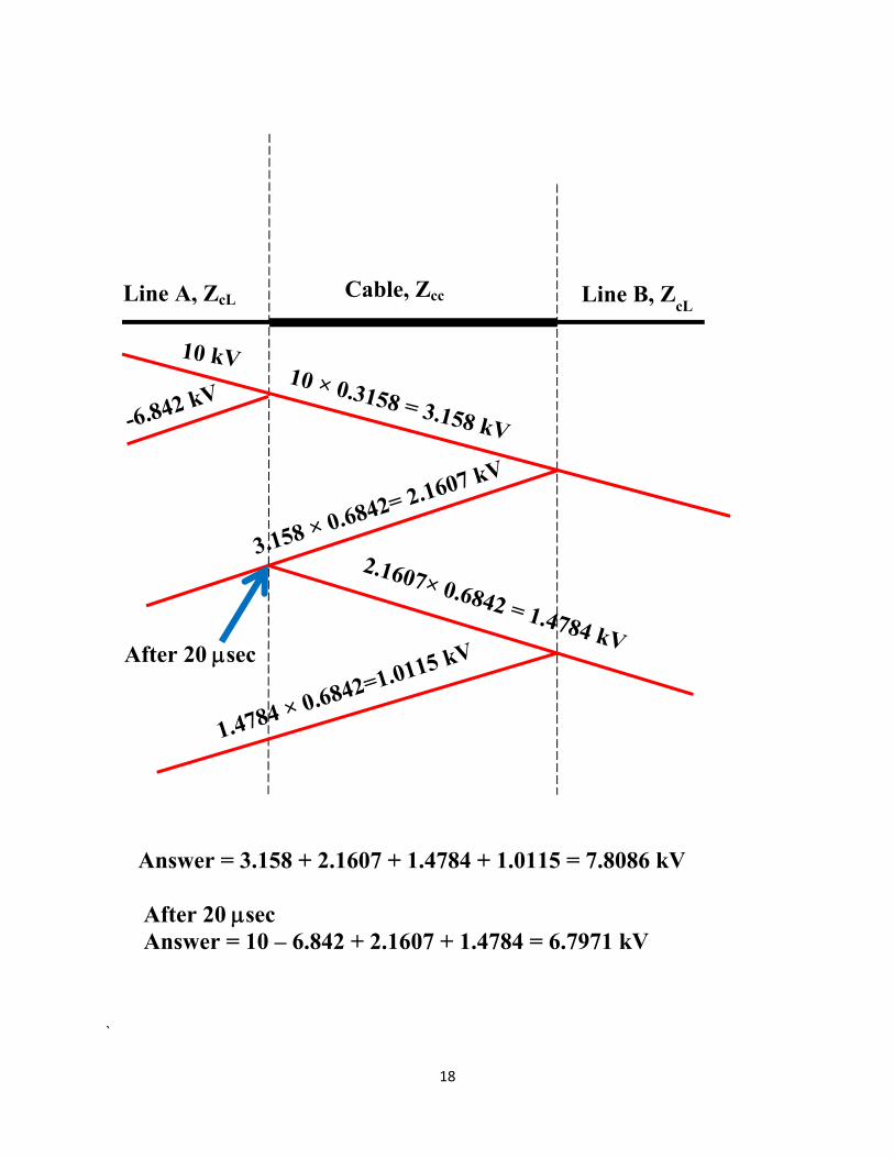
The ends of two long transmission lines A and B are connected by a cable C 1.5 km long. The lines have capacitance of 10 pF/m and inductance 1.6 × 10-6 H/m and the cable has capacitance 89 pF/m and inductance 5× 10-7 H/m. A rectangular voltage wave of magnitude 10 kV and of long duration travels along line A towards the cable. Find the magnitude of the second voltage step occurring at the junction of the cable and line B. What will be the voltage at the junction of line A and the cable 20 sec after the initial surge reaches this point?

17

= 1.6 × 1010 × 10 = 400 Ω

= 5 × 1089 × 10 = 75 Ω

From line A to cable

Transmission operator = = × = 0.3158 From cable to lines A and B

Reflection operator: Γ = = = 0.6842

From line A to cable

Reflection operator: Γ = = = −0.6842

Surge velocity in the cable = 1√ = 1√5 × 10 × 89 × 10= 149906.3378 / Time of travelling through the cable

= 1.5149906.3378 = 10

18

`

Line A, ZcL Cable, Zcc Line B, ZcL

Answer = 3.158 + 2.1607 + 1.4784 + 1.0115 = 7.8086 kV

After 20 sec Answer = 10 – 6.842 + 2.1607 + 1.4784 = 6.7971 kV

After 20 sec

19

Example: A 500 kV surge on a long overhead line of characteristic impedance 400 Ω, arrives at a point where the line continues into a cable AB of length 1 km having a total inductance of 264 H and a total capacitance of 0.165 F. At the far end of the cable, connection is made to a transformer of characteristic impedance 1000 Ω. The surge has negligible rise-time and its amplitude may be considered to remain constant at 500 kV for a time-longer than the transient times involved here.

Draw the Bewley lattice diagram at the junction A of the cable for 26.4 sec after the arrival at this junction of the original surge.

= 264 × 100.165 × 10 = 40 Ω

Velocity of the surge through the cable: = 1√264 × 10 × 0.165 × 10 = 151515.2 /

Time for the surge to travel through the cable: t = 1151.5152 = 6.6

From Line to cable:

Transmission operator = = × = 0.1818 Reflection operator: Γ = = = −0.8182

From Cable to Line:

Reflection operator: Γ = = = 0.8182

Line Cable Transforme

20

Transmission operator = = × = 1.8182 From cable to transformer

Reflection operator: Γ = = = 0.9231

90.9 kV up to 13.2 sec, 243.46 kV from 13.2 to 26.4 sec, rising to 358.69 kV at 26.4 sec.

Transformer

Overhead line, Zc1 Cable, Zc2

Junction Reflection 0.9231

21

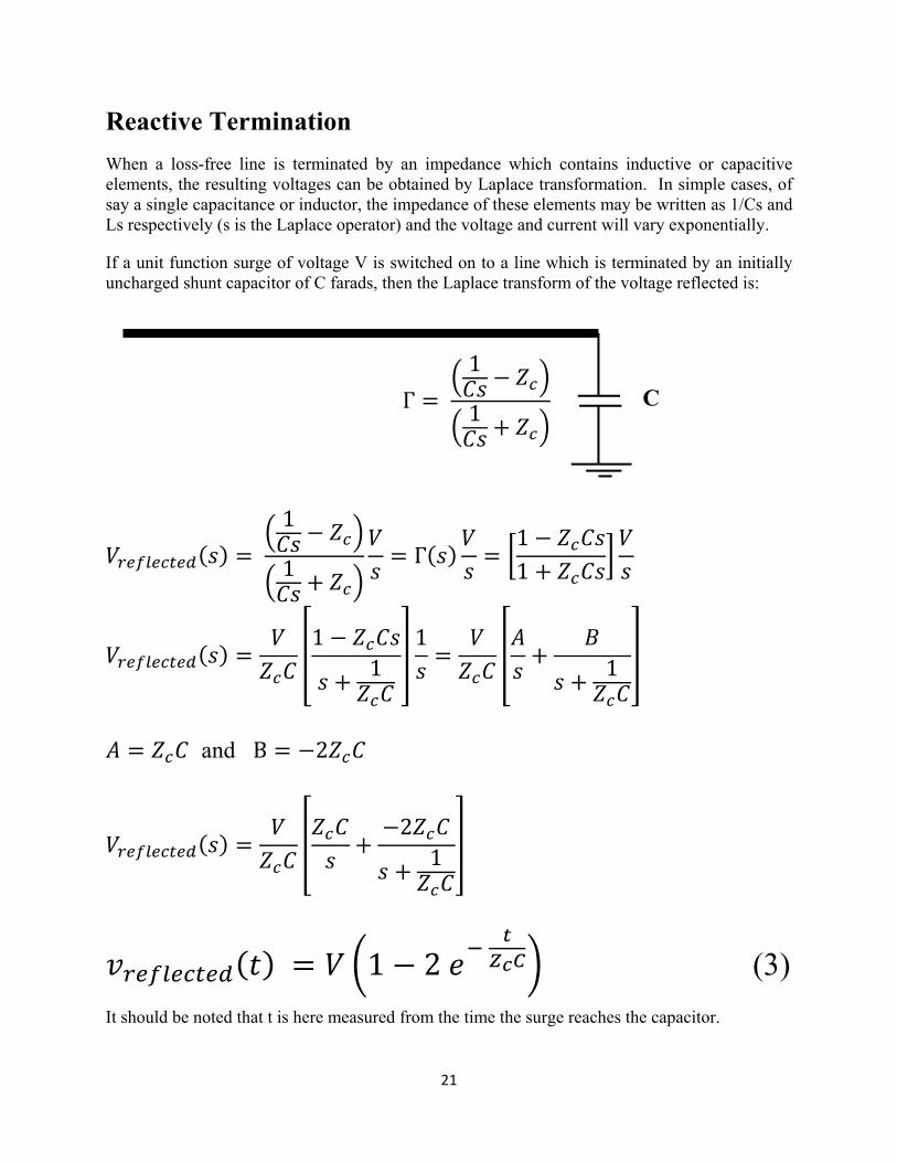
Reactive Termination

When a loss-free line is terminated by an impedance which contains inductive or capacitive elements, the resulting voltages can be obtained by Laplace transformation. In simple cases, of say a single capacitance or inductor, the impedance of these elements may be written as 1/Cs and Ls respectively (s is the Laplace operator) and the voltage and current will vary exponentially.

If a unit function surge of voltage V is switched on to a line which is terminated by an initially uncharged shunt capacitor of C farads, then the Laplace transform of the voltage reflected is:

= 1 −1 + = Γ = 1 −1 +

= 1 −+ 1 1 = + + 1

= and B = −2 = + −2+ 1

= 1 − 2 (3)

It should be noted that t is here measured from the time the surge reaches the capacitor.

Γ = 1 −1 + C

22

The voltages and currents are illustrated in the figure below. The currents follow from I = V/Zc , = − and the above vreflected equation. The distributions of voltages and current shown in

this figure and the time variations of voltage given by Equation (3) might have been deduced from the fact that the applied surge is assumed to be of infinitely steep wavefront so that it contains a range of frequencies extending to infinity. The capacitor, therefore, acts initially as a short-circuit so that the reflected wave is negative and brings the voltage at that point to zero. The capacitor then charges up with a time constant of CZc until, when completely charges, it constitutes an open circuit and the voltage is then 2V.

Voltages and currents at a capacitor line termination.

The corresponding case of a shunt inductor of L Henrys gives the transform reflected voltage as

ℒ = −+ = 1 − 2 +

= −1 + 2 (4)

The voltage and current distributions are shown in the figure below. The voltages and current for this case are the duals of those for the capacitor termination. At the instant the surge arrives the inductor appears as an open circuit so that the voltage doubles. The current increases exponentially from zero in L until finally it corresponds to a short-circuit if the resistance of the inductor is negligible.

23

Voltages and currents at an inductive line termination.

Example:

A rectangular surge of 100 kV and 20 sec duration travels along a line of surge impedance 500 Ω and 100 km long with a velocity of 3×108 m/sec, towards the end of the line which is terminated with a 0.02 F capacitor. Calculate the maximum voltage appearing across the capacitor. = 0.02 × 10 × 500 = 1 × 10 = 100 1 − 2 ×× = 72.9329

Maximum voltage = 100 + 72.9329 = 172.9329 kV

Γ = −+ L

24

Reflection and Refraction at a Bifurcation

Let a line of natural impedance Z1 bifurcate into two branches of natural impedances Z2 and Z3, then, as far as the voltage wave is concerned, the transmitted wave will be the same for both branches, since they are in parallel. On the other hand, the transmitted currents will be different in the general case of Z3 ≠ Z2. A short time after reflection the condition will be as shown in Figure B-1 in which it is assumed that the voltage is reflected with reversal of sign.

Figure B.1: Effect of a bifurcation on the travelling waves.

Z1

Z3

E E’’

E’’

Z2

E’

I

I2

I2

25

Let E1, I1 be the incident voltage and current

E’, I’ be the reflected voltage and current

E’’, I2 be the transmitted voltage and current along Z2

E’’, I3 be the transmitted voltage and current along Z3

Then = and =

Also − = +

The solution of which is

= 21 + 1 + 1

Knowing E1, all the other quantities can be calculated. If we put Z3 = ∞ in the above expression, we have = 2 +

The case becoming that of a simple junction of two lines having different characteristics.

Example

An overhead transmission line having a surge impedance of 450 ohms runs between two substations A and B; at B it branches into two lines C and D, of surge impedances 400 and 50 ohms respectively. If a travelling wave of vertical front and magnitude 25 kV travels along the line AB, calculate the magnitude of the voltage and current waves which enter the branches at C and D.

26

Incident voltage = E1 =25000 V

Incident current = I1 = E1/Z1 = 25000/450 = 55.6 A

Transmitted voltage along BC and BD

= 21 + 1 + 1

×

Transmitted current along BC:

I2 = E’’/Z2 = 4500/400 = 11.25 A

Transmitted current along BD:

I3 = E’’/Z3 = 4500/50 = 90 A

Thus, the current reflected back into line AB = 90 + 11.25 – 55.6 = 45.65 A

Z1 = 450 Ω

E1 C

B

A

Z2 = 400 Ω

Z3 = 50 Ω