Work supported in part by US Department of Energy contract DE-AC02-76SF00515.

Transmission and Radiation of an Accelerating Mode ina Photonic Bandgap Fiber

C.-K. Ng, R. J. England, L.-Q. Lee, R. Noble, V. Rawat and J. SpencerSLAC National Accelerator Laboratory

2575 Sand Hill Road, Menlo Park, CA 94025, USA

Abstract

A hollow core photonic bandgap (PBG) lattice in a dielectric fiber can provide high gradi-ent acceleration in the optical regime, where the accelerating mode resulting from a defect inthe PBG fiber can be excited by high-power lasers. Efficient methods of coupling laser powerinto the PBG fiber are an area of active research. In this paper, we develop a simulation methodusing the parallel finite-element electromagnetic suite ACE3P to study the propagation of theaccelerating mode in the PBG fiber and determine the radiation pattern into free space at theend of the PBG fiber. The far-field radiation will be calculated and the mechanism of couplingpower from an experimental laser setup will be discussed.

1 Introduction

The photonic bandgap fiber proposed by Lin [1] has shown through simulation the possibility ofconfining an accelerating mode in an energy band gap existing in a periodic lattice of vacuumholes with a defect located in the center. Such fibers can in principle achieve high gradients whenoperated in the optical regime using lasers for excitation of the accelerating mode. However, themechanism of coupling power into the PBG fiber has not been addressed. Conventional microwaveaccelerating structures use metallic waveguides for coupling power from external power sources.In the microwave regime, an accelerating structure is normally connected to beampipes at bothends so that the accelerating mode is confined in the structure for a standing wave or propagatesin the forward direction for a traveling wave. In the optical to infrared regime, the power cannotbe delivered through a metallic waveguide for distances L � 200 wavelengths because of thelarge wall loss at high frequencies, and thus an optical fiber waveguide should be considered. It isalso important that the power coupling into the PBG fiber will propagate in the forward directionalong the beam direction using the traveling, defect mode for acceleration. In order to understandthe complexities involved in designing a coupler for the PBG fiber, it is instructive to study boththe transmission and radiation pattern from the propagation of the accelerating mode in the PBGfiber through numerical simulation, which will provide insights for the mechanism of exciting the

1

SLAC-PUB-14156

accelerating mode in an experimental setup. The details of coupler designs using optical fiberwaveguides will be reported in a subsequent paper [3].

This work will focus on numerical simulations of the propagation of the defect mode in the PBGfiber and from the fiber into free space. We use the electromagnetic simulation package ACE3P [2]developed at SLAC for the simulations. ACE3P is a suite of parallel electromagnetic codes basedon the finite-element method, and it consists of solvers in both the frequency and time domains.There are several advantages of using these codes for our simulations. First, tetrahedral finite el-ements with quadratic curved surfaces are well suited for modeling the curved geometries of thePBG fiber with high fidelity. The finite elements also have higher-order basis function representa-tions which allow solutions with high accuracy. Second, the simulation of the propagation of theaccelerating mode requires its excitation at a port boundary of the computational volume. The elec-tromagnetic field pattern of the defect mode can be solved by the frequency-domain eigensolverOmega3P [4] in ACE3P, and then loaded into the time-domain solver T3P [5], where appropriateboundary conditions can be imposed on the outer surfaces of the computational volume to termi-nate the propagation of electromagnetic waves. Third, the parallel capability of these codes allowslarge problems to be solved on parallel computers. This is useful for simulating the radiation intofree space from the accelerating mode by using a large computational volume.

This paper is organized as follows. In section 2, we use the frequency-domain eigensolverOmega3P to determine the defect mode in the PBG fiber. In section 3, we describe a numericalprocedure to simulate the propagation of the defect mode traveling in the PBG fiber using the time-domain code T3P. In section 4, we calculate the power radiated from the accelerating mode intofree space and determine the far-field radiation pattern. A summary of the results is given in thelast section.

2 Defect Mode in Photonic Bandgap Fiber

The PBG fiber (see Fig. 1) proposed by Lin consists of circular holes in a lattice with spacing abetween the centers of neighboring holes, and hence the resulting lattice has a 6-fold symmetry.The holes have a radius of 0.35a. In order to introduce a defect in the lattice, one hole is replaced byanother with a radius of 0.52a. The material of the fiber has a dielectric constant of 2.13. In Lin’spaper, the defect mode is obtained using the Plane Wave Method [6] with the propagation constantβ = kz/k0 = 1, where k0 and kz are the wave number and its component along the propagation z-axis, respectively. Here we used Omega3P, a Maxwell eigensolver that was developed to solve forthe resonant modes of an accelerator cavity. The simulation uses a thin slab of the PBG fiber withcircular cross section, which is truncated at five lattice constants from the center of the defect. Byimposing different boundaries conditions at opposite sides of the slab, the frequencies of standingwave modes are obtained with their wavelengths determined by the slab thickness. Omega3Psolves for a number of modes above a certain specified frequency, and the defect mode can beidentified from the field patterns of these modes. By repeating the simulation for different slabthickness, the frequency of the defect mode as a function of the propagation constant is obtained.

2

Figure 1: One quarter of the Lin PBG structure where a defect hole is located at the center in alattice consisting of regularly spaced holes of the same size.

The dispersion curve is shown in Fig. 2, from which the frequency of the synchronous modepropagating at the speed of light is found to be 8.2c/a, the same as that obtained in Ref. [1].

Figure 2: Dispersion curve calculated by Omega3P near the PBG defect mode.

The longitudinal and transverse electric field patterns, and the transverse magnetic field patternare shown in Fig. 3. All relevant figures in this paper use a rainbow color scheme to representmagnitude with the red and blue being the maximum and minimum, respectively. It can be seenthat the defect mode is TM-like with a uniform distribution of longitudinal field inside the defecthole that can be used for acceleration. All the field components exhibit the six-fold symmetry ofthe lattice, with their maxima located at a distance 1-1.5 a from the center of the defect. The valuesof the transverse electric and magnetic fields at different locations of the cross section of the PBG

3

fiber obtained from Omega3P are written to files which will then be read in as inputs to the timedomain solver T3P for studying mode propagation. It is instructive to see how the defect modeis confined by studying the decay of its electromagnetic fields from the center of the defect hole.Fig. 4 shows the variations of the longitudinal component of the electric field as a function of thetransverse position (in units of a) along the x-axis and y-axis. The field decays to very small value(less than several % of the maximum) when the distance is bigger than 4a in both directions. Inthe defect hole, the field remains essentially constant. This is in good agreement with the resultsobtained in Ref. [1].

Figure 3: Defect mode in the PBG fiber: (a) longitudinal electric field; (b) transverse electric field;(c) transverse magnetic field.

Figure 4: Variations of the longitudinal electric field of the defect mode along the x-axis and y-axis.

4

3 Propagation of Defect Mode

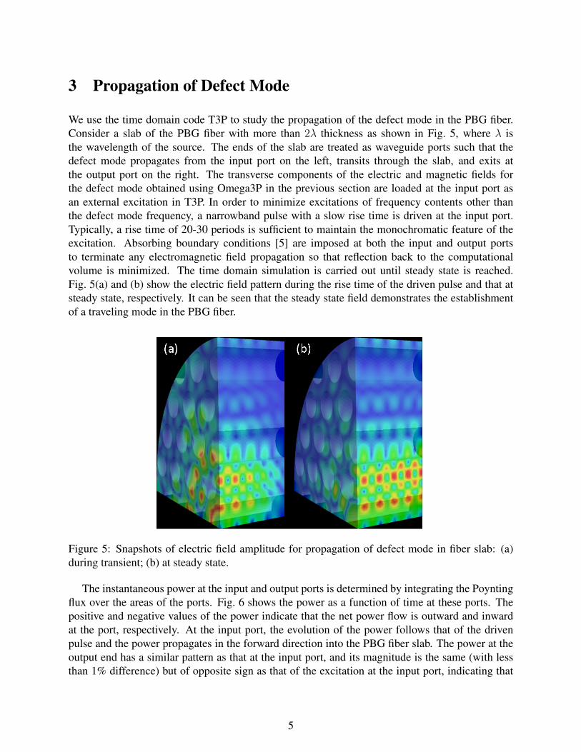
We use the time domain code T3P to study the propagation of the defect mode in the PBG fiber.Consider a slab of the PBG fiber with more than 2λ thickness as shown in Fig. 5, where λ isthe wavelength of the source. The ends of the slab are treated as waveguide ports such that thedefect mode propagates from the input port on the left, transits through the slab, and exits atthe output port on the right. The transverse components of the electric and magnetic fields forthe defect mode obtained using Omega3P in the previous section are loaded at the input port asan external excitation in T3P. In order to minimize excitations of frequency contents other thanthe defect mode frequency, a narrowband pulse with a slow rise time is driven at the input port.Typically, a rise time of 20-30 periods is sufficient to maintain the monochromatic feature of theexcitation. Absorbing boundary conditions [5] are imposed at both the input and output portsto terminate any electromagnetic field propagation so that reflection back to the computationalvolume is minimized. The time domain simulation is carried out until steady state is reached.Fig. 5(a) and (b) show the electric field pattern during the rise time of the driven pulse and that atsteady state, respectively. It can be seen that the steady state field demonstrates the establishmentof a traveling mode in the PBG fiber.

Figure 5: Snapshots of electric field amplitude for propagation of defect mode in fiber slab: (a)during transient; (b) at steady state.

The instantaneous power at the input and output ports is determined by integrating the Poyntingflux over the areas of the ports. Fig. 6 shows the power as a function of time at these ports. Thepositive and negative values of the power indicate that the net power flow is outward and inwardat the port, respectively. At the input port, the evolution of the power follows that of the drivenpulse and the power propagates in the forward direction into the PBG fiber slab. The power at theoutput end has a similar pattern as that at the input port, and its magnitude is the same (with lessthan 1% difference) but of opposite sign as that of the excitation at the input port, indicating that

5

the power flows out from the PBG fiber. There is a time delay between the input and output signalsdetermined by the group velocity of the traveling wave, which is found to be 0.61c, in agreementwith that obtained in Ref. [1].

Figure 6: Power transmission in the PBG fiber slab. The blue and red curves represent the inputand output pulse, respectively.

4 Simulation of Radiation from Defect Mode

4.1 Radiation from Defect Mode

To provide insights of how to couple power into the PBG fiber, it is instructive to study the inverseproblem first, namely the radiation pattern from the propagation of the defect mode into free space.The radiation pattern will provide guidelines to project laser beams near the end of the PBG fiberto excite the defect mode. To this end, we use the time domain code T3P to simulate the modelas shown in Fig. 7. Because of symmetry, only one quarter of the PBG fiber is simulated. In thismodel, a PBG slab is placed in a spherical volume whose spherical surface is terminated using anabsorbing boundary condition so that the outgoing waves diffracted at the interface between thePBG fiber and the vacuum will not be reflected back into the computational volume. In a similarmanner as discussed in the previous subsection, the defect mode is excited at the input port locatedat the left end of the PBG slab, propagates through the slab, and then radiates into free space.Again, to maintain the monochromatic feature of the pulse, a slow rise time is used similar to thatin the previous section. In contrast to the previous case of wave propagation in a uniform PBG

6

slab, the smooth propagation of the electromagnetic fields of the defect mode will be intercepted atthe PBG-vacuum interface. Part of the power carried by the defect mode will be reflected and therest will transmit out the right hand boundary of the PBG and radiate into free space. The radiatedelectromagnetic waves will be terminated at the surrounding spherical surface for the simulation.

Figure 7: Snapshot of the radiated electric field from the propagation of the defect mode in thefiber. In the simulation, the length of the fiber slab is a little bigger than 2λ and the radius of thesphere enclosing the simulation model is 10λ.

A snapshot of the electric field amplitude at steady state is shown in Fig. 7. It can be seen thatthe radiated field propagates in a non-uniform manner with power confined in several cones withcertain solid angles. The detail of the distribution will be discussed later. The electric field insidethe PBG fiber shows the modulation of the forward traveling wave as a result of the reflection atthe PBG-vacuum interface. The diffracted wave has an extended high field region shown in redand is located at a distance of about one wavelength in the forward direction along the symmetryaxis (z) of the fiber that is due to the constructive interference of the uniform field of the acceler-ating mode scattering from the exit of the circular defect aperture. The field distributions on theplane perpendicular to the z-axis are shown in Fig. 8 with the electric field still showing stronglongitudinal polarization components. Notice that there are other components of the radiation fieldthat are barely visible in Fig. 7 that we will discuss further in Fig. 10.

Fig. 9 shows the power radiated out at the spherical surface of the computational volume, and

7

Figure 8: The amplitudes of (a) the electric field and (b) the magnetic field at a distance of aboutone λ from the PBG-vacuum interface. The cones represent the field vectors and their sizes scaleas the magnitudes of the fields.

that reflected back into the PBG fiber. The positive and negative values of the power indicatepower flowing outward and inward through a surface, respectively. The time evolution of theinstantaneous power at the output spherical surface shows that the electric and magnetic fields ofthe radiated waves are not in phase, indicating that interference effects from the diffracted wavesat this distance are still important to preclude the establishment of a far field radiation pattern. Thepositive values of the instantaneous power at the input port mean that some power is reflected andpropagates backward in the PBG fiber. The averaged radiated and reflected power is found to beabout 81% and 19%, respectively.

Fig. 10 shows the radiation pattern on the spherical surface, looking from the longitudinal axisof the PBG fiber. This represents one quarter of the forward hemisphere. Two prominent peaks inthe Poynting flux can be seen on the surface. The location of each peak is defined by two angles (θ,φ), where θ is the angle between the longitudinal z-axis and the line joining the peak location andthe origin defined at the fiber-vacuum interface, and φ defined by the projection on the transversex-y plane of the PBG fiber. Both peaks are located at θ = 45o from the longitudinal, symmetryz-axis and the two transverse angles φ are at 0o and 60o with respect to the x-axis (Fig. 10).

4.2 Far-field Radiation Pattern

Following the procedure in the previous subsection, one can obtain the far-field radiation patternon the spherical surface by using a forward hemisphere with a large radius � λ. However thecomputational domain will become very big and the calculation will be very time-consuming. Tocircumvent this problem, we opt to extract the fields on the plane of the fiber-vacuum interface anduse them as excitation sources in calculating the far-field radiation. Fig. 11 shows the electric andmagnetic fields on this plane. The field patterns at this plane preserve most of those of the defectmode shown in Fig. 3.

8

Figure 9: Radiated power (red) and power transmitted at the input port (blue) for the propagationof the defect mode at the end of the fiber.

Figure 10: Radiated power pattern in the forward quarter spherical surface (with a radius of 8a orabout 10λ) from defect mode propagation in the fiber.

9

Figure 11: The amplitudes of (a) the electric field and (b) the magnetic field at the PBG-vacuuminterface. The cones represent the field vectors and their sizes scale as the magnitudes of the fields.

The far-field radiation is determined using Huygen’s Principle [7] and obtained through thefollowing procedure. The source plane is divided into a number of patches using a rectangular grid.Within each grid, the current sources are calculated using the electric and magnetic field vectorsobtained from the T3P simulation. Since only a quarter of the structure is simulated in T3P, thesource plane representing the full model is obtained by reflecting appropriately the fields throughthe symmetry planes. The display surface of the far-field radiation is chosen to be a forwardhemisphere with its origin at the defect center. The distant spherical surface is also divided into anumber of patches, the dimensions of which are set to 0.2λ. The far-field radiation in each patch isdetermined by all the patches in the source plane through the propagation of the electromagneticradiation in free space. Thus the computation for the far-field on the whole surface scales asthe product of the numbers of the patches in the source plane and radiation surface. A Matlabpropagator code [8] was used for the calculation, and the choice of 0.2λ resolution for the surfacepatches is found to be sufficient to reveal the radiation pattern within a reasonable amount ofcomputational time.

Fig. 12 shows the Poynting flux of the far-field radiation on the hemispherical surface as afunction of the radius R of the hemisphere, scaled to the same size for ease of display. Theradiation pattern changes drastically from R = 5λ to R = 20λ and reaches a steady configurationat R = 80λ. It should be noted that the radiation pattern at 10λ is very similar to that obtained bydirect T3P simulation where the radius of the spherical surface enclosing the computation domainis 10λ. Using the source fields determined by a different code [9] for PBG mode calculation andpropagating these with the Matlab code shows similar radiation patterns as those shown in Fig. 12,verifying qualitatively the correctness of our calculations. As shown from Fig. 12, the far-fieldradiation pattern has a six-fold symmetry and is localized in the hot spot regions (indicated byred color) on the downstream surface. Remembering that the z-axis is in the forward directionperpendicular to the source plane, the centers of the hot spots are located at θ = 45o from thez-axis, and spaced at 60o in the azimuth φ. This angular dependence agrees well with that obtainedfrom direct simulation using T3P (Fig. 10). To estimate the spatial extent of a hot spot on the

10

Figure 12: Projection of Poynting flux from the surface of the forward hemisphere onto a circulardisk (scaled) as a function of the hemisphere radius at 5λ, 10λ, 20λ, 40λ, 80λ and 120λ.

Figure 13: Poynting flux on the surface of the forward hemisphere with radius 80λ. The z-axis isnormal to the source plane, and the x- and y-axes define the source plane.

11

surface as shown in the 3-dimensional plot at R = 80λ in Fig. 13, the boundary of the region isdefined by the Poynting flux value dropped by two e-foldings of the maximum. It is found that thesix hot spots together contain 75% of the radiated power within 33% of the total surface area.

Figure 14: Variations of Poynting flux along the longitude and latitude passing the peak of a hotspot on the forward hemisphere with radius 80λ. The variation along the latitude covers a rangeof 60o, the angle of rotation symmetry of the radiation pattern. The variation along the longitudespans from 0-90o but is predominately confined to about 30o and is shifted by 45o so that its peakcoincides with that along the latitude for easy comparison.

Figure 14 shows the variations of the Poynting flux along the longitude and latitude passingthrough the peak of a hot spot on the forward hemisphere with radius 80λ. It can be seen thatthe shape along the longitude is very close to a Gaussian and the variation along the latitude israther linear in nature. Figure 15 shows the shape of the hot spot along the longitude and latitudefor different hemisphere radii R from 10λ to 120λ. The shape along the longitude is alwaysnarrower than that along the latitude. Along the longitude, the width of the Gaussian-like shapegets narrower as R increases until it reaches a steady state above 80λ. Along the latitude, the shapeis rather Gaussian-like at R = 10λ, after which it broadens out with a double-humped profile andchanges back to a broad peak with linear drops on both sides when R is greater than 80λ. Thisillustrates the complicated interference effects contributed by the current sources as one movesaway from them. A brief word about radiation and coupling effects in such fiber may be usefulhere before proceeding because the two are clearly related. For the types of modes of concern here,losses from the sides and ends need to be considered and while these have different fixes, they areboth defined by the basic hexagonal symmetry of the lattice. Thus, losses from both sides and endstypically show six-fold symmetry and will be addressed in a subsequent paper where perturbationsof the pure hexagonal lattice symmetry about the defect is broken in various periodic and aperiodic

12

ways.

Figure 15: The shapes of a hot spot along (a) the longitude and (b) the latitude for different hemi-sphere radii (in units of λ).

Fig. 16 shows the polarizations of the electric and magnetic fields at one of the hot spot locatedin the projected horizontal x-direction. The electric field vectors point towards the pole of thehemisphere along a longitude, and the magnetic field vectors along a latitude on the surface. Thepolarizations at other hot spots behave in a similar manner by rotating φ = 60o with respect to thez-axis. The far-field polarizations are reminiscent of those of the spherical TM01 mode, but havestrong localized magnitudes in the six hot spots for the PBG fiber, with an E×H structure similarto a laser’s TEM beam. Therefore, as a reverse process, six laser beams with their polarizations inphase can be used as a means to direct power from a far distance (≈ 120λ) to excite the acceleratingmode in the PBG fiber.

5 Conclusion

The PBG fiber proposed by Lin [1] has shown through simulation the existence of a defect modethat can be used for particle acceleration. The coupling of power from external power sources hasto be efficient in order that the PBG can be a potential candidate for future linear colliders usinglasers as excitation sources. We have developed the numerical methods through the parallel elec-tromagnetic finite-element code suite ACE3P to simulate the propagation of the accelerating modeinside the PBG fiber and determine its far-field radiation pattern. The far-field Poynting flux re-flects the six-fold symmetry of the geometry of this PBG fiber with the radiated power concentratedin six localized regions. From the polarizations of the radiated fields, the lasers can be aligned inthese localized regions to direct power to the PBG fiber to excite the accelerating mode efficiently.This would be the first major step in coupling power to the PBG fiber for the demonstration of laseracceleration. This appears to be a comparatively easy and efficient technique to excite these modesin a way that does not interfere with the simultaneous injection of the particle bunches. Alternate

13

methods of directly coupling power into the PBG fiber using waveguide structures in the opticalregime are under study [3] and may provide better efficiency for acceleration.

Figure 16: Polarizations of electric (a) and magnetic (b) fields in the far right hot spot (φ = 60o,θ = 45o) of the far-field radiation shown in Fig. 12 for the hemisphere radius at 80λ.

Acknowledgements

We would like to thank Eric Colby for many useful discussions and use of his Matlab code, andGreg Schussman for help with visualization. The work was supported by the U.S. DOE contractDE-AC02-76SF00515. The work used the resources of NCCS at ORNL which is supported by theOffice of Science of the U.S. DOE under Contract No. DE-AC05-00OR22725, and the resourceof NERSC at LBNL which is supported by the Office of Science of the U.S. DOE under ContractNo. DE-AC03-76SF00098.

References

[1] X. E. Lin, Phys. Rev. ST Accel. Beams 4, 051301 (2001).

14

[2] ACE3P: An Advanced Computational Electromagnetic SimulationSuite, https://confluence.slac.stanford.edu/display/AdvComp/ACE3P+-+Advanced+Computational+Electromagnetic+Simulation+Suite.

[3] R. J. England et al., Calculation of Coupling Efficiencies for Laser-Driven Photonic BandgapStructures, Proc. of 2010 Advanced Accelerator Concepts Workshop.

[4] L.-Q. Lee et al., Omega3P: A Parallel Finite-Element Eigenmode Analysis Code for Acceler-ator Cavities, Tech. Report, SLAC-PUB-13529, 2009.

[5] A. E. Candel et al., Parallel Higher-Order Finite Element Method for Accurate Field Com-putations in Wakefield and PIC Simulations, Proceedings of International Computational Ac-celerator Physics Conference, Chamonix Mont-Blanc, France, 2006.

[6] K. Leung and Y. Liu, Phys. Rev. Lett. 65, 2646 (1990).

[7] L. Diaz and T. Millagan, Antenna - Engineering Using Physical Optics, Artech House, Inc.,1996.

[8] E. Colby, private communications.

[9] B. Kuhlmey, CUDOS MoF Utilities for micro-structured optical fibres, University of Sydney,Australia. http://www.physics.usyd.edu.au/cudos/mofsoftware.

15