transit competitiveness in polycentric metropolitan regions

Transportation Research Part A 41 (2007) 19–40

www.elsevier.com/locate/tra

Transit competitiveness in polycentricmetropolitan regions

Jeffrey M. Casello

School of Planning and Department of Civil Engineering, University of Waterloo,

200 University Avenue West, Waterloo, Ont., Canada N2L 3G1

Abstract

This paper analyzes the potential to, and impacts of, increasing transit modal split in a polycentric metropolitan area –the Philadelphia, Pennsylvania region. Potential transit riders are preselected as those travelers whose trips begin and endin areas with transit-supportive land uses, defined as ‘‘activity centers,’’ areas of high-density employment and trip attrac-tion. A multimodal traffic assignment model is developed and solved to quantify the generalized cost of travel by transitservices and private automobile under (user) equilibrium conditions. The model predicts transit modal split by identifyingthe origin–destination pairs for which transit offers lower generalized cost. For those origin–destination pairs for whichtransit does not offer the lowest generalized cost, I compute a transit competitiveness measure, the ratio of transit general-ized cost to auto generalized cost. The model is first formulated and solved for existing transit service and regional pricingschemes. Next, various transit incentives (travel time or fare reductions, increased service) and auto disincentives (higherout of pocket expenses) are proposed and their impacts on individual travel choices and system performance are quantified.The results suggest that a coordinated policy of improved transit service and some auto disincentives is necessary toachieve greater modal split and improved system efficiency in the region. Further, the research finds that two levels of coor-dinated transit service, between and within activity centers, are necessary to realize the greatest improvements in systemperformance.� 2006 Elsevier Ltd. All rights reserved.

Keywords: Polycentric cities; Activity centers; Multimodal modeling; Traffic assignment; Modal split; Transit competitiveness; Mobility

1. Introduction

In the last half of the 20th century, North American urban development patterns have become greatly dis-persed. The trend began in the post war period with a heavy migration of residential activities outside of tra-ditional urban cores. Later, in the 1970s and 1980s, employers followed seeking generally lower rents andaccess to more highly educated labor. While residential activities were generally low-density, commercial ven-tures tended to be more clustered, as a result of land use controls and forces off agglomeration.

0965-8564/$ - see front matter � 2006 Elsevier Ltd. All rights reserved.

doi:10.1016/j.tra.2006.05.002

E-mail address: [email protected]

mailto:[email protected]

20 J.M. Casello / Transportation Research Part A 41 (2007) 19–40

In the 1990s many of these commercial clusters have expanded to form ‘‘activity centers,’’ locations of con-centrated employment outside of urban cores. Regions with several activity centers in addition to the tradi-tional downtown are referred to in the literature as polycentric metropolitan areas. These areas presentnew challenges for transportation professionals to plan, design and operate efficient transportation systems.

Briefly, polycentric cities compared to traditional monocentric urban areas tend to exhibit more distributedtrip patterns, more reliance on private automobile and less use of public transportation and non-motorizedmodes. These characteristics can result in negative transportation system performance, including occurrencesof regional congestion and mobility limitations for some part of the population.

This paper analyzes the potential to improve overall system performance by increasing public transporta-tion ridership in polycentric metropolitan areas, using the Philadelphia Pennsylvania region as a test case. Theapproach taken here is to preselect travelers whose origin and destination pairs are strong candidates for pub-lic transportation, and whose normal auto path consumes capacity on regionally congested links. The disutil-ity of travel by transit and private auto is quantified using a multimodal traffic assignment model. Aftermodeling and calibrating the base-case situation, alternative policies are explored to provide transit incentives,to implement auto disincentives, and to combine these policies. For each alternative, the model is solved andchanges in transit ridership and system performance are quantified.

The results demonstrate that an integrated, regional approach addressing transit competitiveness for tripsbetween and within activity centers can reduce congestion and increase mobility in metropolitan areas.

2. Literature review

The concept of polycentric metropolitan areas has been researched extensively in many fields. One commoncharacteristic is the need to identify areas outside of traditional urban cores that represent ‘‘activity centers,’’or nodes in the polycentric region. Quantitative definitions largely grew out of regional economic literature,and as such, are largely based on total employment and employment density. Briefly, there are two commonapproaches to quantifying activity centers. The first method, typically attributed to McMillen and McDonald(1997), uses sophisticated methods to identify areas that exhibit statistically significant deviations in employ-ment from surrounding zones. The second approach, traditionally attributed to Giuliano and Small (1991),sets a priori threshold levels for both employment and employment density; geographical areas (typicallyTAZs) which exceed these values belong to activity centers. Casello and Smith (accepted for publication) haveproposed a modification to the Giuliano and Small approach that includes a trip attraction weighting for thedisaggregate employment types present in a potential activity center. The authors call these areas Transpor-tation Activity Centers. That research identified 21 suburban activity centers in the Philadelphia metropolitanarea, four of which serve as inputs to the model used here.

A substantial body of research exists on transportation patterns associated with activity centers. NCHRP(1989) analyzed six suburban activity centers in the United States to develop a comprehensive database ontravel characteristics: origins, destinations, trip purpose, length and mode. TRB (1990) measured suburbancongestion, evaluated suburban trip generation and modal split, and enumerated policy needs for more effi-cient activity centers. Cervero (1989) identified 57 suburban activity center sites throughout the United Statesfrom which he developed tremendous aggregate data on the transportation infrastructure that support theseSACs. Cervero and Wu (1998) have done targeted analysis on the San Francisco metropolitan area. Modarres(2003) presents an excellent literature review of activity center transportation analysis in his work analyzingpublic transportation access to disaggregate employment types within Los Angeles’ activity centers.

Kuby et al. (2004) analyzed more than 200 Light Rail Transit (LRT) station to determine which land use ornetwork characteristics were effective predictors of ridership. Their intention was to identify if LRT couldattract sufficient ridership in polycentric metropolitan areas. Their conclusions include that ‘‘a station neednot be downtown to generate substantial ridership,’’ that employment was a statistically significant variablein attracting riders, and similar factors explained ridership at CBD and non-CBD stations.

Boile and Spasovic (2000) and Boile (2002) first proposed the use of multimodal traffic assignment modelsto evaluate the impacts of changes in pricing on modal split. The work presented here relies heavily on theseformulations; the extension to their work is to recognize the positive correlation between land use density and

J.M. Casello / Transportation Research Part A 41 (2007) 19–40 21

transit ridership established by Pushkarev and Zupan (1982), TCRP (1996) and Nelson/Nygard (1995) inselecting origin and destination pairs.

3. Activity centers identification and analysis

The goal of this research is to examine how public transportation may improve regional transportation sys-tem performance. The intent is to identify travelers whose origin and destination pairs are well served by pub-lic transportation, and whose trip path consumes critical regional highway infrastructure. As noted above,activity centers are areas of high density of development; prior research suggests that transit’s competitivenessincreases as land use density increases. Thus, trips originating and destined for regional activity centers arestrong candidates to increase transit modal split and to improve system performance.

3.1. Identifying critical activity centers

Casello and Smith (accepted for publication) have identified 21 suburban activity centers, two secondaryurban centers and three major urban centers in the Philadelphia metropolitan area. These centers representareas of not only high-density employment, but also concentrated trip attraction within the region. While itis feasible to include all these centers in the subregional model developed here, a subset of these centers areselected based on the following observations. Improving transit modal split produces the most positiveimpacts for trips utilizing congested highway infrastructure. Furthermore, reducing congestion is most desir-able on the highest-volume regional links, as delay reductions on these links result in the greatest absolute timesavings and the greatest reduction in negative externalities. Thus, this model analyzes trips associated with asubset of activity centers which are adjacent to congested, high-volume regional roadways.

Fig. 1. Philadelphia metropolitan area and major highway sections.


The Philadelphia region is served by the following major highways, shown in Fig. 1:

1. Interstate 95, running north–south adjacent to the Delaware River.2. The Pennsylvania Turnpike, composed of routes I-276 and I-76, running east–west through the region.3. Interstates 676 and 76 (known locally as the Schuylkill Expressway), from Camden, New Jersey through

downtown Philadelphia westward, connecting to both Interstate 476 to the north and Interstate 276 tothe west.

4. Interstate 476, connecting I-95 south of the city to I-76 and I-276 northwest of the city.5. US 202 which acts as a suburban beltway along the western border of the metropolitan region.6. US 422, the fastest growing corridor in the region, extending the Philadelphia suburbs to the northwest.

Recurrent congestion occurs on several of these highways. SEPTA (2001) using 1997 Annual Average DailyTraffic (AADT) estimates notes that during peak periods I-76 eastbound and westbound operate at Level ofService (LOS) E or F along the corridor between center city Philadelphia and the interchange with I-276. Thesame study found that US 422 operates at LOS F both eastbound and westbound for approximately five milesfrom its intersection with US 202. The six mile segment of US 202 northbound and southbound betweenNorristown and King of Prussia is also operating under unstable or failure conditions.

Based on this study’s findings, the Schuylkill Expressway, US 202 and US 422 appear to be primary cor-ridors on which improving the highway performance may have the greatest regional impacts. The impacts ofother regional roadways, such as I-476 and I-276, on these major regional routes’ performance should also beconsidered. These critical highways either pass through or are adjacent to eight of the activity centers identifiedin Casello and Smith (accepted for publication). These centers are shown as the shaded areas in Fig. 2.

Fig. 2. Philadelphia metropolitan area with the eight activity centers considered.


3.2. Trips associated with the identified activity centers

Table 1 shows the daily trips between the eight activity centers. The total number of trips is shown, aswell as trips disaggregated into three categories: home based work (HBW), home based non-work (HBNW),non-home based (NHB) for the eight activity centers studied in the Philadelphia region. The data shown wereprovided by Walker (2003) and are the output of that agency’s regional travel model. DVRPC models a ‘‘com-bined peak’’ period including trips made between 7:00 a.m. and 9:00 a.m. and 3:00 p.m. and 6:00 p.m. Thismodel disaggregates time of day sensitive parameters such as freeway capacity and transit service parametersto better reflect the peak period. The output trip table from this combined peak period for the eight activitycenters is shown in Table 2.

3.3. Observations on trip volumes

The trip volumes presented in Tables 1 and 2 offer some insight into the Philadelphia region’s travel pat-terns. For commuting trips, home based work trips during peak hours, Center City dominates as a destination,

Table 1Daily trip table for the eight activity centers considered

Camden Center City Fairmount West Phila City Line Consh – PM Norristown King of Prussia

Total daily trips

Camden 4656 726 91 90 29 9 6 15Center City 360 90,500 5760 10,540 2258 276 114 278Fairmount 96 11,949 4414 2340 547 63 30 73West Phila 58 11,787 1555 5441 609 62 29 62City Line 45 6698 825 1416 7080 272 106 264Consh – PM 20 1567 135 241 362 18,005 2490 2338Norristown 16 1223 102 191 224 3682 12,635 8575King of Prussia 9 412 44 72 123 819 2151 38,864

Daily non-home based

Camden 3627 204 38 28 12 5 4 5Center City 200 50,221 3519 6050 1540 146 69 127Fairmount 35 3449 1880 845 228 19 7 16West Phila 29 5859 890 3284 378 28 13 24City Line 11 1531 234 381 3997 109 41 73Consh – PM 6 191 23 37 113 7848 992 562Norristown 5 70 11 15 36 994 4013 1563King of Prussia 6 150 20 31 82 555 1528 29,096

Daily home based work

Camden 398 454 45 56 16 2 1 6Center City 124 15,960 997 2143 367 67 30 85Fairmount 51 4511 745 854 158 24 16 33West Phila 23 2934 269 812 115 17 12 21City Line 25 2987 286 578 575 69 35 83Consh – PM 12 1155 91 172 172 1339 525 627Norristown 11 1027 83 153 151 907 2038 2078King of Prussia 3 234 19 37 35 110 208 1233

Daily home based non-work


Table 2Combined peak period trip table for the eight activity centers considered

Camden Center City Fairmount West Phila City Line Consh – PM Norristown King of Prussia

Total combined peak

Camden 1454 319 38 37 10 3 2 6Center City 134 31,069 1898 3423 667 80 36 88Fairmount 32 4723 1568 938 194 22 11 30West Phila 22 4112 499 1918 200 19 8 20City Line 19 2726 319 571 2543 82 36 86Consh – PM 8 675 56 105 129 6345 813 787Norristown 8 542 41 85 91 1259 4738 3229King of Prussia 2 153 17 25 37 222 626 11,776

Peak non-home based


Peak home based work

Camden 222 245 23 29 6 1 1 3Center City 65 8744 539 1126 190 26 15 38Fairmount 23 2463 410 454 83 12 7 18West Phila 13 1580 145 452 61 9 5 10City Line 13 1621 157 315 336 33 18 39Consh – PM 6 576 45 86 84 812 287 331Norristown 6 494 38 74 73 494 1218 1181King of Prussia 1 112 9 16 16 56 115 725

Peak home based non-work

Camden 215 22 3 1 0 1 0 1Center City 13 8183 393 708 99 16 1 20Fairmount 1 1323 618 262 47 5 3 8West Phila 3 970 119 479 38 5 1 5City Line 3 712 100 151 968 25 9 30Consh – PM 0 56 6 9 18 3190 275 322Norristown 0 32 1 8 11 517 2328 1629King of Prussia 0 7 2 1 0 38 122 2866


with nearly 60% of all peak period trips ending in that activity center. More broadly, the combination of WestPhiladelphia, Fairmount and Center City accounts for almost 75% of total trip destinations in the peak per-iod. There exists, however, a strong commuting pattern among the suburban activity centers (Conshohocken/Plymouth Meeting, Norristown, and King of Prussia). For example, from Norristown the number of trips des-tined for King of Prussia is nearly 2.5 times as high as the number of trips from Norristown destined for Cen-ter City. Similarly, an equal number of trips from Norristown are destined for Plymouth Meeting as aredestined for Center City.

These volumes suggest that commuting patterns are not simply radial from the suburbs into the centralbusiness district, but rather contain a strong inter-suburban component. Table 3 summarizes commuting pat-terns for these eight activity centers based on whether the origin and the destination are suburban (the threecenters defined above plus City Line Avenue) or urban (Camden, Center City, Fairmount and WestPhiladelphia).

The data in Table 3 shows that 22% of all commuting trips associated with these eight activity centers beginand end within a suburban activity center, while only 13.5% begin in a suburban center and end in an urbancenter. Table 3 also suggests that currently there is little evidence of a strong ‘‘reverse commute,’’ with only1.8% of trips beginning in an urban activity center and ending in a suburban activity center.

Table 3Urban–suburban commuting patterns for the Philadelphia region

Origins Destinations

Urban Suburban

Urban 16,533 (62.6%) 485 (1.8%)Suburban 3569 (13.5%) 5818 (22.0%)


Considering non-home based trips (NHB), several additional observations are possible. First, the totalnumber of NHB trips during the peak period is greater than the number of HBW trips. It is reasonable toassume that a significant portion of these peak period NHB trips occurs as an intermediate stop during themorning or afternoon commute – trip chaining.

A second observation is that intra-center trips account for more than 77% of all NHB trips that occur in thepeak period. This value is significantly higher than for HBW trips, where 49% of trips are intra-center. Sim-ilarly, less than 7% of NHB trips go between an urban activity center and a suburban activity center. If theassumption that most peak NHB trips are intermediate commuting stops is extended, the high number ofintra-center trips implies that most trip chaining occurs near either the origin or the destination. This suggeststhat mixed use development that supports non-motorized modes (i.e. Transit Oriented Development, TOD)might be effective in accommodating this trip demand and reducing the number of vehicular trips in a region.

Lastly, the King of Prussia activity center generates and attracts a disproportionate number of NHB trips.Intra-King of Prussia trips account for approximately 2.8% of the total commuting (HBW); intra-King ofPrussia trips account for more than 21.3% of total NHB trips. This is partially explained by the presenceof a regional shopping center in the area, the King of Prussia Plaza and Court which together have 2.9 millionsquare feet of gross leasable area (GLA) (Philadelphia Business Journal, 2003).

4. Modeling transit competitiveness and system performance

A multimodal traffic assignment model is used to quantify the disutility of travel at user equilibrium for allmodes. At equilibrium, transit competitiveness can be quantified for the origin–destination pairs identifiedabove. Impacts of policy and operational changes for both transit and auto travel on modal split and systemperformance can be directly computed from the output of the model. Components of this model include thefollowing:

1. The trip table (trip volumes by origins and destinations – from Tables 1 and 2);2. A representation of the transportation infrastructure in link – node format, including pertinent link vari-

ables such as: capacity, length, free-flow travel time and tolls;3. A measure of traveler disutility for each mode;4. A representation of ‘‘external’’ traffic, that is traffic that does not originate or is not destined for the sub-

regional area, but consumes transportation infrastructure capacity;5. A representation of transit service, including waiting time, in-vehicle travel time, and fare (out of pocket

expense);6. A traffic assignment algorithm that is known to converge to equilibrium;7. Model calibration, to ensure that the model output accurately reflects the transportation network

conditions.

These model components are discussed in the following sections.

4.1. Peak hour trip table

The trip table for this study is computed by converting the DVRPC peak period (5 h) trip volumes to asingle peak hour volume. The Highway Capacity Manual (Transportation Research Board, 1985) gives severalgraphs of hourly variations on different classifications of roadways. The HCM examples suggest ranges from


nearly uniform peak periods, with 20% of total volume occurring in the highest peak hour, to a sharply peakedcondition where nearly 40% of peak period traffic occurs in the highest-volume hour. Given this range of val-ues, and the intention of this modeling effort to evaluate congested freeway conditions, it is assumed that 40%of the peak period trips occur in the peak hour.

4.2. Network representation

The network infrastructure representation is shown in Fig. 3. Freeway sections are shown as solid lines,while principal arterials are represented as lighter weight dashed lines. Nodes 1–56 are actual intersectionsof highways. Nodes 58, 60 and 61 are centroids of the Center City, Fairmount and Camden centers, respec-tively. Nodes 64–70 are TAZ centroids used to model the trips within the Norristown activity center. Similarly,nodes 71–76 are origins and destinations for trips internal to the Plymouth Meeting activity center; nodes 77and 78 serve the same purpose for the King of Prussia Center. Nodes 79–82 are the centroids of the King ofPrussia, Norristown, Plymouth Meeting and City Line Avenue centers, respectively. Node 84 serves as thecentroid to the West Philadelphia center.

The model also represents intra-zonal trips for those TAZs with intra-zonal flows greater than 500 trips perhour. For example, more than 10,000 trips originate and end within one TAZ (node 78) in the King of Prussiacenter during the combined peak period. To model these trips, three additional source/sink nodes (nodes 85–

Fig. 3. Model representation of the highway infrastructure.


87) are created within the TAZ. A similar approach is taken for two additional TAZs within the PlymouthMeeting center.

Note that no internal travel is modeled for the urban centers. It is assumed that the modal split for tripswithin these centers is sufficiently high, and that non-motorized modes serve these trips particularly well. Tripsto and from the urban centers are included in the model to represent the volume these trips add to the sub-urban activity center traffic.

The resulting network is one with 90 nodes and 192 links (384 directional) representing more than 191 (382)kilometers of highway. Of these links, 204 represent highways; 48 are imaginary, zero cost links connectingcenter or intra-center centroids to the transportation network. An additional 132 links represent transit con-nections within and between activity centers.

The capacity of each link is taken from DVRPC (2000) models. The DVRPC has three capacity values(high, medium, low) for each highway class and for each Area Type through which the highway carries traffic.For this model, a single rounded mean capacity value is used for each highway functional class. Lengths ofeach link are calculated by hand using large-scale commercially available maps. Free-flow travel time is com-puted using the distances and speeds based on DVRPC (2000) recommended speed for each functional class.

4.3. Auto traveler disutility

The total cost experienced by a driver is computed as a function of travel time, travel distance, and out ofpocket expenses. Travel time is calculated using the Bureau of Public Roads formulation (Bureau of PublicRoads, 1964). Estimating the value of travel time has been the subject of extensive research (see, for example,the Victoria Policy Institute, 2002; Villain and Bhandari, 2002; Cohen and Southworth, 1999; Small andWinston, 1999; USDOT, 1997). Estimates vary greatly depending on, primarily, locality. There are, however,several points upon which researchers agree. First, commuters have the highest value of time; second, thevalue of time increases with personal income; finally, commuter’s travel time should be estimated as a functionof local wages and benefits. Given these criteria, the assumed value employed in this model formulation is $25per hour. This value is within the limits of empirically derived values in the referenced studies and is consistentwith the upper end of commuters’ salaries and benefits. The model uses this value of time for all trips occurringin the peak hour.

The cost of travel per unit distance is assumed to be $0.15 per vehicle kilometer. This value is intended torepresent only fuel cost and operation under congested conditions. Out of pocket expenses include tolls andparking. Tolls are only present in the submodel on two links representing the Pennsylvania Turnpike and onRoute 676 connecting Camden to Philadelphia. The cost of trips along these links is incorporated in themodel. Additional out of pocket expenses are included for parking for trips that are destined for nodes withinthe urban activity centers.

4.4. Model calibration – modeling external trips

A major challenge in developing and calibrating the model is to represent trips external to the activity cen-ters. These trips are necessary to ensure that links are operating with sufficient volume to match observed con-ditions. Further, changes in system performance, increases and decreases in travel times, are experienced notonly by the travelers associated with the activity centers but also by external users.

The methodology used here to represent the external trips is to assign iteratively an artificial, bidirectionaltravel demand for trips between each origin–destination pair that defines a link in the network proportional tothe capacity of the connecting link. For example, the link defined as connecting nodes 1 and 2 has a capacity of1200 vehicles per hour; external traffic is modeled as a demand between nodes 1 and 2 of 1080 trips, in this case90% of capacity. This approach allows the artificial demand to be the primary calibration tool. Moreover, byadding artificial demand between nodes, the model solution actually assigns these trips to the lowest costroute. In other words, the external demand between link end-points may not be accommodated by only thelink between them, but may also seek lower cost paths through the network.

After several iterations, it was determined that an external travel demand equal to 90% of link capacityresulted in a sufficiently accurate representation performance. Several O–D pairs connected by links which


are chronically congested were assumed to have slightly larger demands. For example, link 9–63 (and link 63–9) is one of the most frequently congested roadway sections in the region; the demand for travel between nodesnine and 63 is assumed to be 95% of the capacity of link 9–63.

A summary of the model formulation is shown in Table 4.

4.5. Modeling transit service

Transit service between activity centers is typically modeled as artificial links between the centroids of zones(Sheffi, 1985); that approach is taken here. The total generalized cost of transit time is computed as a functionof the access time to the transit service within a TAZ, the waiting time which is calculated based on the line’sheadway, in-vehicle travel time, and the fare. Access time is calculated for each TAZ based on transit’s areacoverage within the zone and the quality of vehicle and pedestrian access to the transit system. Waiting time isassumed to be one-half of the headway up to a maximum value of 10 min for single seat trips on rail systems.For bus systems, the waiting time is one-half the headway with a maximum of 10 min for headways up to

Table 4Summary of network modeling approach

#Nodes: 90

• 62 roadway intersections• 8 center centroids• 15 TAZ centroids• 5 intra-zonal sources

#Links: 384

• 102 ‘‘real’’ (204 directional)• 24 centroid connectors (48 directional)• 56 inter-center transit connections• 76 intra-center transit connections

Total distance modeled:

• 382 km

Travel time equation:

• FFTT � 1þ 0:25vc

� �b� �

ð1Þ

• where FFTT is the free-flow travel time, v is volume, c is capacity and b is an estimated parameter

Link parameters: free-flow speeds (kilometers per hour), capacities (vehicles per hour – lane), b (from (1))

• Freeway: 100, 2000, 7• Expressway: 85, 1400, 7• Arterial: 50, 800, 7• Ramps: 60, 1140, 7• Centroid connectors: 100, 10,000, 1

Travel costs:

• Value of IVTT: $25 per hour• Cost associated with distance: $0.15 per kilometer• Parking costs:

– Center City $7 per trip– Camden $7 per trip– Fairmount $5 per trip– W. Phila. $3 per trip

# Trips modeled:

• 20,503 ‘‘real trips’’ in peak hour• External trips added on links such that

vc

P 0:90


30 min. For headways greater than 30 min, the waiting time is assumed to be 1/3 the headway with a maxi-mum value of 15 min. These estimates have a significant shortcoming. Using this formula, increasing a head-way from 30 min to 1 h only imposes a 5-min additional waiting time on transit service. This penaltyunderestimates the added inconvenience of delayed (or earlier) travel. This methodology, however, is the stan-dard practice and is adopted here.

A traveler experiences two waiting times on trips requiring a transfer. The model reflects this combinedwaiting cost by calculating the first waiting time as described above. The second waiting time, associated withthe transfer, is computed as one-half the minimum of the two line’s headways.

The in-vehicle travel time is computed based on published transit operator schedules including the Southeast-ern Pennsylvania Transit Authority (SEPTA) and the Delaware River Port Authority’s PATCO service betweenCenter City Philadelphia and Camden, New Jersey. It is assumed that these published schedule times (PST)include typical transit passenger volumes. Higher transit volumes will likely cause only marginal increases in tra-vel time. As such, the transit link travel times are computed using the BPR function, with very high capacity. Onlyin the case of very high volumes does the travel time significantly depart from published schedules.

Transit service within the suburban activity centers is modeled based on existing service; as an example,Fig. 4 shows the existing transit service in the King of Prussia area and its model representation. Inter-centertransit travel times, types and fares are shown in Table 5. A summary of the transit modeling approach isshown in Table 6.

4.6. Equilibrium traffic assignment solution methodology

Many traffic assignment models exist that have been shown to reach equilibrium (Patriksson, 1994). Theassignment algorithm used here was developed and coded by Bar-Gera (2002). The model is solved to

Fig. 4. King of Prussia activity center transit service.

Table 5Transit connection matrix showing in-vehicle travel time, service type, and fare

Camden Centralbusinessdistrict

Fairmount WestPhiladelphia

CityLine

PlymouthMeetingConshohocken

Norristown King ofPrussia

CAM – 14 min 22 min 19 min 50 min 80 min 57 min 77 minPatco Patco – HR Patco – HR Patco – Bus Patco – Bus Patco – RR Patco – Bus$1.15 $2.20 $2.20 2.45 $3.56 $4.03 $4.13

CBD 14 min – 8 min 5 min 34 min 66 min 43 min 61 minPatco HR HR Bus 1 Bus RR 1 Bus$1.15 $1.30 $1.30 $1.30 $2.41 $2.88 $2.88

FM 22 min 8 min – 13 min 42 min 72 min 47 min 69 minHR – Patco HR 2 HR HR – Bus HR – Bus Bus – RR HR – Bus$2.20 $1.30 $1.30 $1.59 $2.41 $2.88 $2.88

WP 19 min 5 min 13 min – 31 min 80 min 47 min 63 minHR – Patco HR 2 HR HR – Bus HR – Bus HR – HSL HR – Bus$2.20 $1.30 $1.30 $1.59 $2.41 $2.41 $2.88

CLA 50 min 34 min 42 min 31 min – 46 min 41 min 58 minBus – Patco Bus Bus- HR Bus – HR 2 Bus Bus – RR 2 Bus$3.56 $1.30 $1.59 $1.59 $1.59 $1.59 $1.93

PM 80 min 66 min 72 min 80 min 46 min – 31 min 60 minBus – Patco 1 Bus Bus – HR Bus – HR 2 Bus Bus 2 Bus$3.56 $2.41 $2.41 $2.41 $1.59 $1.30 $1.93

NT 57 min 43 min 47 min 47 min 41 min 31 min – 33 minRR – Patco RR RR – Bus HSL – HR RR – Bus Bus 1 Bus$4.03 $2.88 $2.88 $2.41 $1.59 $1.30 $1.30

KOP 77 min 61 min 69 min 63 min 50 min 60 min 33 min –Bus – Patco 1 Bus Bus – HR Bus – HR 2 Bus 2 Bus 1 Bus$4.13 $2.88 $2.88 $2.88 $1.93 $1.93 $1.30

HR = heavy rail.

Table 6Summary of transit modeling cost components and assumptions

Total travel cost

• Value of Travel time * (Access time + Waiting time + IVTT) + Fare

Access time

• Empirically derived based on: transit area coverage within a TAZ, pedestrian connections, and parking availability at stations

Waiting time assumptions

• Bus systems, single seat ride: WT = h/2, 610 min for h < 30 min; h/3 6 15 min for h > 60 min• Rail system, single seat ride: WT = h/2, 610 min " h

• Either mode with a transfer: Total wait time = WT1 + WT2, where WT1 = Single seat rule; WT2 = 1/2 * min{h1,h2}

In-vehicle travel time (IVTT):

• Empirically derived from published schedules’ times (PST)

• Mathematically modeled as : PST 1þ 0:15v

10; 000

� �� ð2Þ

• Represents transit’s insensitivity to volume

Fares

• ‘‘Per-trip cost’’ calculated as monthly pass cost divided by 44 commuting trips per month



equilibrium using an 800 mHz PC in less than 1 min. Unlike some large-scale models solved with the Franke–Wolfe algorithm, this model solution technique solves to sufficient accuracy (in terms of link flows and costs)to be certain that changes in the model outputs are a result of changes in the system representation.

It is also important to note that because the solution reached is user equilibrium, the results can bedescribed as stable: no individual user has motivation to change his route or mode because no better alterna-tive exists. Naturally, the stability of the results is predicated upon the assumption that the model representshuman behavior sufficiently well. The model which predicts mode choice based on lower generalized cost,including travel time and out of pocket expenses, makes two major assumptions. First, a cost-based modalsplit model ignores captive riders, those for whom auto travel is not possible, and therefore probably under-estimates total transit ridership. In terms of variables included in the mode split model, the literature suggeststhat a series of input variables may be considered (Ben-Akiva and Morikawa, 2002) which may increase (envi-ronmental concerns) or decrease (comfort, safety, etc.) the likelihood of transit ridership. It is unclear if thesimplification of mode choice to include only travel time and out of pocket expenses is likely to overestimateor underestimate transit ridership in the Philadelphia Region.

5. Measures of system performance

This work posits that on a system-wide (macro) level, increasing transit’s modal split for a subset of regio-nal trips can improve the regional transportation system performance; congestion can be reduced resulting inhigher efficiency, lower cost travel. Therefore, to measure the effectiveness of proposed operational, policy ordesign changes, pertinent statistical measures include:

1. Total system cost – the disutility of completing all trips (real and external) throughout the network; withfixed demand calculating total system cost also computes average user cost. Mathematically, total systemcost is given by
X
o

Xd

GC�od � T od where GC�od ¼ minfGCTod;GCA

odg ð3Þ

where GC is the generalized cost from origin (o) to destination (d) by transit (T) and auto (A); Tod is thetravel volume from o to d.

2. The number of transit links used, as a measure of transit’s integration and ubiquity in the transportationnetwork;

3. The total system delay in person-hours. In this case, delay is defined as the increase in link travel time versusthe free-flow travel time. To calculate total delay, the increased travel time is multiplied by the flow on thelink. Mathematically, the delay function is given as

Xi

Xj

FFTTij � avc

� �b� T ij ð4Þ

where FFTTij is the free-flow travel time from i to j; a, b are defined as in the BPR travel time equation; v isthe volume on link i, j; c is the capacity of link i, j; Tij is the flow on link i, j.

4. The transit modal split. The model assigns trips to the lowest cost path for an origin–destination pair. Thepath may be made up of all auto links, a single transit link, or a combination of auto and transit links. Thetransit modal split can be computed as the number of trips assigned to transit links versus the total numberof trips assigned.

5. Transit competitiveness, defined as the ratio of generalized cost of a trip between a given O–D pair by tran-sit and automobile. A ratio greater than one suggests that auto has lower generalized cost. Mathematically,this ratio is given as

Competitiveness ¼ GCTod

GCAod

¼ TTTod � VOTTþ fareod

TTAod � VOTTþ X A

od � 0:15þAuto OOPð5Þ


where TTod is the travel time from the origin to the destination by transit (T) or auto (A) in minutes; VOTTis the value of travel time $ per minute; fare is the transit fare from origin to destination; X is the distancefrom origin to destination in kilometers; Auto_OOP is the auto out of pocket expense in $ per trip.This measure of transit competitiveness has many positive features. The ratio is very easy to compute fromthe model output. Further, because the statistic is a ratio of generalized cost, the assumption regardingvalue of time is somewhat less important.

On a more macro-level, transit competitiveness can be thought of as a measure of mobility. Measuring thegeneralized cost ratios for classifications that correspond to the trip types gives insight into how well transit isserving regions of the metropolitan area. For example, transit competitiveness can be computed for all tripswithin an activity center, or for all trips between suburban centers and urban centers. As transit is more com-petitive for whole groups of trips, the region’s mobility (i.e. travel alternatives) can be said to increase.

In this research, weighted transit competitiveness statistics are computed for:

1. King of Prussia intra-center trips;2. Norristown intra-center trips;3. Plymouth Meeting intra-center trips.4. Urban to suburban inter-center trips (trips beginning in an urban activity center and terminating in a sub-

urban activity center);5. Suburban to urban inter-center trips (trips beginning in a suburban activity center and terminating in an

urban activity center);6. Suburban to suburban inter-center trips (trips beginning in one suburban activity center and ending in a

different suburban activity center).

Mathematically, this weighted average can be expressed as

TableBase-c

Case

Base c

a Mo

1

T Sk

Xo

Xd

T od �GCT

od

GCAod

8o; d 2 Sk and GCTod > GCA

od ð6Þ

where Sk represents the six subsets described above.These macro- and micro-level statistics are used to quantify existing conditions and to evaluate proposed

measures to improve system performance.

6. Summary of base-case results

The peak hour is modeled and calibrated and the base-case results are summarized in Table 7.The total system cost incurred by users of all modes in this peak hour is $631,499. Transit is the lowest cost

alternative for five suburban to urban connections with one intermodal trip. For all other categories, no tran-sit service offers lower disutility than automobile service. The total delay experienced in the system is 6019 per-son-hours. The transit competitiveness ratio for all trips modeled is 4.1.

Further analysis of transit competitiveness for subsets of trips is computed. The maximum ratio for a singleO–D pair, the minimum ratio for a single O–D pair and the weighted average for each of the six categories arepresented in Table 8.

The King of Prussia activity center is made up of two TAZs. One of those TAZs is further divided into foursub-TAZ level model analysis zones – Zone 78 is further subdivided into zones 78, 85, 86 and 87 in Fig. 4.

7ase results

Total system cost Transit modal split (%) Transit links useda Total system delay (h) Transit competitiveness

ase $631,499 7.2 5 6109 4.1

dal split and transit links used is based only on suburban trips.

Table 8Base-case cost ratios for each of the six trip categories

Category Maximum Minimum Weighted

1. King of Prussia intra-center 16.7 1.7 5.22. Norristown intra-center 21.6 3.9 9.03. Plymouth Meeting intra-center 19.0 1.1 4.54. Urban to suburban inter-centers 2.9 1.2 1.85. Suburban to urban inter-centers 1.6 <1 1.36. Suburban to suburban inter-centers 4.2 1.4 2.3System wide 4.1


Thus, the King of Prussia activity center consists of five origins and destinations or 20 O–D pairs. The max-imum observed generalized cost ratio for trips within the King of Prussia activity center is from origin 86 todestination 85 – where transit costs approximately 16.7 times more than auto. The minimum observed general-ized cost ratio for King of Prussia trips is from zone 87 to zone 85, where transit costs only 1.7 times as muchas auto. Overall, for trips within King of Prussia, transit currently offers relatively poor service, costing onaverage 5.2 times as much as automobile travel.

The Plymouth Meeting center shows an even greater disparity in quality of transit service between O–Dpairs, ranging from a maximum of 19.2 to a minimum of 1.3. This implies that for at least one O–D pair withinthe Plymouth Meeting center (76 to 75) transit is completely uncompetitive and for another O–D pair (79 to84) transit cost exceeds auto cost by only 30%. Of the three suburban activity centers, Plymouth Meeting offersthe most competitive transit service (has the lowest weighted average of cost ratios) for intra-center trips, whileNorristown offers the least competitive.

The third column of Table 8 shows the minimum cost ratio for each subset of trips. The lowest value is 1.1for Plymouth Meeting intra-center trips; all subsets have a minimum value less than 1.8 except Norristownintra-center trips where the minimum is 3.9. In general, these low minimum values suggest that there is at leastone origin–destination pair belonging to each trip category for which transit could become competitive withminor pricing or operational changes.

7. Transportation system improvements

In the following sections the existing transportation conditions are modified in an attempt to improve sys-tem performance. The changes are broadly classified into two categories: auto disincentives and transit incen-tives. Auto disincentives are based primarily on increasing the cost of automobile trips; the motivation forthese cost increases is to attribute to the driver a portion of the external costs associated with his trip. Thetransit incentives include lower cost service, faster service (through priority treatment, for example) and theintroduction of new transit service in suburban areas. Finally, a combination of auto disincentives and transitincentives is explored.

7.1. Auto disincentives

Three alternative auto disincentives are considered. First, to represent higher marginal cost of auto travel,the cost per unit distance is increased from the base-case $0.15 per kilometer to a $0.30 per kilometer. Thischange may represent a higher fuel tax, distance-based insurance charges, or perhaps greater use of tolls.The second proposal is to implement a cordon toll of $4.00 for trips entering the city limits. This type of tollcharge had been successfully implemented in Singapore, prior to implementing a larger network of toll collec-tion devices. More recently, London has imposed a cordon toll with very promising results. The last alterna-tive implements a $2.00 fixed charge for all suburban destinations (both activity center destinations and intra-center trips). This charge represents parking fees.

The model is revised to represent these changes and rerun. The macro-output statistics are shown in Table 9.Each of these three pricing changes achieves one of the primary goals, reducing system-wide delay.

The increased distance cost policy is most effective, reducing delay by approximately 386 h or about 6.3%.

Table 9Macro-output statistics for the auto disincentive model runs

Case Totalsystemcost

% Change insystem cost

Transitmodal splita (%)

Transitlinksuseda

Total systemdelay (h)

% Changein delay

Transicompetitiveness

Base case $631,499 N/A 7.2 5 6109 N/A 4.1A1 – Increased distance cost $742,202 17.5 9.1 9 5723 �6.3 3.3A2 – Cordon toll $650,847 3.1 7.8 6 5828 �4.6 3.9A3 – Suburban fixed charge $650,584 3.0 7.8 9 5983 �2.0 2.0

a Modal split and transit links used is based only on suburban trips.


Increasing distance charges also results in the greatest transit modal split for suburban trips (an increase of1.9% over the base case) and the largest number of transit links used. Last, this policy reduces the system-widegeneralized cost ratio on links for which auto is less expensive from 4.0 to 3.3, meaning that on the whole,transit is slightly more competitive with the auto for these trips. As could be expected, increasing auto travelcosts increases the total system cost significantly, in this case by 17.5%.

The cordon toll and suburban fixed charge policies also reduce the network delay by 4.6% and 2.0%, respec-tively. Each policy results in approximately the same transit modal split of 7.8%, a marginal increase over thebase case. The cordon toll results in only one new transit link being used. With suburban fixed charges, fourorigin–destination pairs within the Plymouth Meeting activity center are served best by transit, resulting in atotal of nine transit links being used for suburban trips. The suburban fixed charges is the most effective policyin improving the overall competitiveness of transit on auto-dominated routes, reducing the system-wide costratio from 4.0 to only 2.0.

Auto disincentives are somewhat ineffective in producing substantive improvements in system performance.On the macro-level, no auto disincentive policy reduces system delay by more than 6.3%, and this gain causesa large increase in total system cost. Implementing a suburban parking charge is most effective in increasingtransit’s overall competitiveness (lowers the overall cost ratio), but this policy does not increase transit’s modalsplit. This is largely a result of the high base-case cost ratios shown in Table 7.

7.2. Transit incentives

As with auto disincentives, three transit incentives are explored and compared to the base case. The firstmeasure is to eliminate fares on the transit system. Such a policy aims to match the low marginal cost of auto-mobile travel and to test the elasticity of transit ridership to out of pocket expense. A second measure tested isto increase the operating speed of existing transit service. To this end, in-vehicle travel time is reduced by 10%and 15% for rail service and bus service, respectively. These reductions in travel time could be achieved byoperational changes such as improved vehicle performance (acceleration or deceleration rates, maximumspeeds) or priority signal treatments in mixed traffic. Last, the impacts of high-frequency, high-area coveragetransit service for each suburban activity center are evaluated. Conceptually, this service could be minibusesoperating on 10 min headways between high traffic generators within the activity centers. Each of these alter-natives is coded and the model is resolved. The macro-output statistics are shown in Table 10.

Table 10Transit incentive macro-outputs

Case Totalsystem cost


Transitmodal splita (%)

Transitlinks useda

Totalsystemdelay (h)

% Changein delay

Transitcompetitiveness

Base case $631,499 N/A 7.2 5 6109 N/A 4.1T1 – Free transit $607,843 �3.8 12.6 8 5492 �10.1 3.5T2 – Increased operating speed $623,519 �1.6 8.6 5 5717 �6.4 3.8T3– Suburban distribution $627,889 �0.9 7.9 8 5857 �4.1 2.8



As with the auto disincentive policies, each of the transit incentive policies increase the transit modal splitand in turn reduce the system-wide delay. The most effective policy in both respects is the free transit alterna-tive which increases transit modal split by 5.4%, makes transit the lower cost alternative on three additionalroutes and decreases system delay by 617 person-hours (10.1%). Logically, eliminating transit fare reduces thetotal system cost by 3.8% as transit riders do not pay a fare and auto users experience less congestion. Increas-ing transit’s operating speed marginally reduces the total system cost (1.6%), increases transit modal split(1.4%) and decreases system delay (6.4%).

The introduction of suburban distribution service – high speed, high-frequency service within each of thesuburban activity centers – produces very small benefits in terms of system cost and system delay reductions,approximately 1% and 4%, respectively. Transit modal split also increases only marginally, by less than 1%, asthese circulator services are lowest cost only on several lightly traveled suburban O–D pairs.

As expected, lowering the cost of transit relative to the automobile increases transit’s competitiveness ineach case. The most effective policy for increasing transit competitiveness is introducing the suburban distri-bution service, followed by implementing free transit and lastly increasing operating speed. These findings sug-gest that in-vehicle travel time and fare are less of a deterrent to suburban transit use than insufficient service:poor area coverage and very long headways.

To summarize, transit incentives fail to produce substantive changes in system performance. Substantialsystem-wide delays remain, and total system cost is reduced by only 4% with free transit. The most promisingcase for improving transit’s system-wide competitiveness is the suburban distributor service, as the weightedcompetitiveness index is reduced from 4.0 in the base case to 2.8.

Given the marginal improvements in system performance realized by the auto disincentive and transitincentive policies independently, it is logical to test combinations of these policies. Two cases are considered.The first case is the combination of suburban fixed charges and improved transit service. Ideally, revenueraised through parking charges could finance the introduction of a competitive transit alternative.

These changes are coded into the model, and the model is rerun. The results are shown in Table 11.This combined policy of dissuading suburban auto use and providing a suitable transit alternative causes 22

additional transit links to be used over the base case and increases the transit modal split by nearly 7%. Ofthese 22 new links, 18 serve Plymouth Meeting intra-center trips and four serve King of Prussia intra-centertrips. Transit serves over 17% of both centers’ intra-center trips. Delay in the system is reduced by almost 12%.The total system cost increases by less than one percent as reductions in travel time nearly offset the increasedparking charges for suburban destinations.

This alternative focuses on the provision of ubiquitous suburban transit service. As a result, this alternativehas a more pronounced effect on the weighted auto path cost ratio, reducing the value from 4.1 in the base caseto 1.6. This suggests for those routes on which the auto remains more competitive, transit service on averagecosts only 60% more.

7.3. The Schuylkill Valley Metro

The Schuylkill Valley Metro (SVM) is a proposed 100-km long transit line to connect Center City Phila-delphia and Reading, Pennsylvania serving essentially the I-76 and US 422 corridors. As shown in Fig. 5,

Table 11Results of the combined auto disincentive and transit incentive model run

Case Total systemcost


Transitmodalsplita (%)

Transitlinksuseda


% Changein delay


Base case $631,499 N/A 7.2 5 6109 N/A 4.1C1 – Combined fixed charges

and suburban distribution$636,546 0.5 14.0 27 5392 �11.7 1.6


Fig. 5. Schuylkill Valley Metro (SVM) alignment.


the proposed alignment would provide service between the centroids of Center City, City Line Avenue,Norristown and King of Prussia. The proposed line would also pass through the Plymouth Meeting activitycenter, but at a significant distance from the zone centroid. The locally preferred alternative is to operate highfrequency (for transit units per peak hour) ‘‘MetroRail’’ service – a high efficiency (high platforms, self-servicefare collection, etc.) electrified light rail system along ROW A for most of the proposed alignment. This oper-ation would substantially reduce travel time for inter-center trips.

This level of transportation investment, as well as the proposed implementation time, would certainlyweaken the applicability of the model developed here. Regional land use and travel patterns would changeconsiderably, making the assumption of a constant O–D matrix in light of the transportation improvementhighly questionable. Despite these concerns, the model is coded to represent SVM service in the corridor,understanding the obvious limitations on the findings. The results are shown in Table 12.

Table 12Results of Schuylkill Valley Metro service

Case Totalsystem cost



Transitlinks useda


% Changein delay


Base case $631,499 N/A 7.2 5 6109 N/A 4.1SVM – Schuylkill Valley Metro $603,512 �4.7 15 11 5159 �15.6 4.0


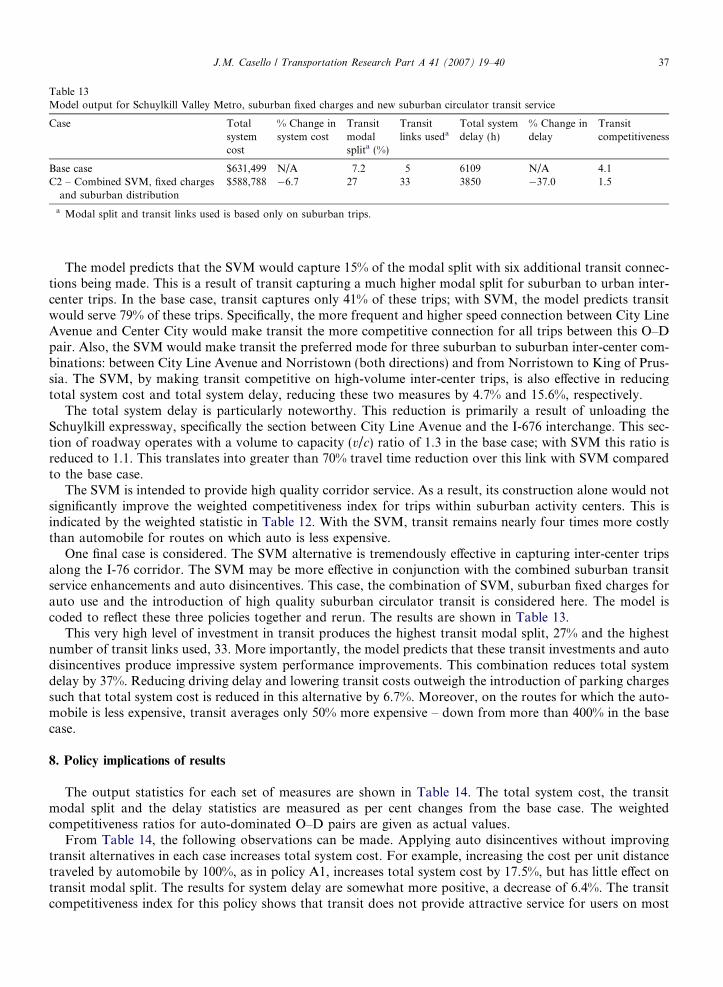
Table 13Model output for Schuylkill Valley Metro, suburban fixed charges and new suburban circulator transit service

Case Totalsystemcost



Transitlinks useda


% Change indelay


Base case $631,499 N/A 7.2 5 6109 N/A 4.1C2 – Combined SVM, fixed charges

and suburban distribution$588,788 �6.7 27 33 3850 �37.0 1.5



The model predicts that the SVM would capture 15% of the modal split with six additional transit connec-tions being made. This is a result of transit capturing a much higher modal split for suburban to urban inter-center trips. In the base case, transit captures only 41% of these trips; with SVM, the model predicts transitwould serve 79% of these trips. Specifically, the more frequent and higher speed connection between City LineAvenue and Center City would make transit the more competitive connection for all trips between this O–Dpair. Also, the SVM would make transit the preferred mode for three suburban to suburban inter-center com-binations: between City Line Avenue and Norristown (both directions) and from Norristown to King of Prus-sia. The SVM, by making transit competitive on high-volume inter-center trips, is also effective in reducingtotal system cost and total system delay, reducing these two measures by 4.7% and 15.6%, respectively.

The total system delay is particularly noteworthy. This reduction is primarily a result of unloading theSchuylkill expressway, specifically the section between City Line Avenue and the I-676 interchange. This sec-tion of roadway operates with a volume to capacity (v/c) ratio of 1.3 in the base case; with SVM this ratio isreduced to 1.1. This translates into greater than 70% travel time reduction over this link with SVM comparedto the base case.

The SVM is intended to provide high quality corridor service. As a result, its construction alone would notsignificantly improve the weighted competitiveness index for trips within suburban activity centers. This isindicated by the weighted statistic in Table 12. With the SVM, transit remains nearly four times more costlythan automobile for routes on which auto is less expensive.

One final case is considered. The SVM alternative is tremendously effective in capturing inter-center tripsalong the I-76 corridor. The SVM may be more effective in conjunction with the combined suburban transitservice enhancements and auto disincentives. This case, the combination of SVM, suburban fixed charges forauto use and the introduction of high quality suburban circulator transit is considered here. The model iscoded to reflect these three policies together and rerun. The results are shown in Table 13.

This very high level of investment in transit produces the highest transit modal split, 27% and the highestnumber of transit links used, 33. More importantly, the model predicts that these transit investments and autodisincentives produce impressive system performance improvements. This combination reduces total systemdelay by 37%. Reducing driving delay and lowering transit costs outweigh the introduction of parking chargessuch that total system cost is reduced in this alternative by 6.7%. Moreover, on the routes for which the auto-mobile is less expensive, transit averages only 50% more expensive – down from more than 400% in the basecase.

8. Policy implications of results

The output statistics for each set of measures are shown in Table 14. The total system cost, the transitmodal split and the delay statistics are measured as per cent changes from the base case. The weightedcompetitiveness ratios for auto-dominated O–D pairs are given as actual values.

From Table 14, the following observations can be made. Applying auto disincentives without improvingtransit alternatives in each case increases total system cost. For example, increasing the cost per unit distancetraveled by automobile by 100%, as in policy A1, increases total system cost by 17.5%, but has little effect ontransit modal split. The results for system delay are somewhat more positive, a decrease of 6.4%. The transitcompetitiveness index for this policy shows that transit does not provide attractive service for users on most

Table 14Summary of policy and operational changes and their system impacts

Measures Total systemcost (% change)

Transit modalsplit (% change)

Delay(% reduction)


Base case N/A N/A N/A 4.1A1 – Increased cost per unit distance 17.5 1.9 6.3 3.3A2 – Cordon toll 2.7 0.6 4.6 3.9A3 – Suburban fixed charge 2.7 0.6 2.1 2.0T1 – Free transit �4.1 5.4 10.1 3.5T2 – Increased operating speed �1.6 1.4 6.4 3.8T3 – Suburban distributor service �0.9 0.7 4.1 2.8SVM – Schuylkill Valley Metro �4.7 7.8 15.6 4.0C1 – Suburban fixed charge and new suburban service 0.5 6.8 11.7 1.6C2 – SVM, suburban fixed charge

and new suburban service�7.1 19.8 37 1.5


routes; on average transit remains 3.3 times as expensive as auto on auto-dominated routes. Similar results areshown for policies A2 and A3. These findings suggest that road pricing solutions alone, when not combinedwith improved transit services, may not achieve the desired system benefits of reduced congestion or improvedoverall system performance.

Each of the three transit incentives measures – eliminating transit fares (T1), increasing operating speeds(T2) and introducing new transit service (T3) reduces the total system costs, increases transit modal splitand decreases the system delay. Measure T1 is most effective of these three policies in reducing delay anddecreasing system cost, while T2 is second and T3 is least effective in these measures. The results suggest thatpolicy T3 will have only a marginal impact on modal split, but a more significant impact on transit compet-itiveness. The weighted index with measure T3 is 2.8, the lowest index of all transit incentive policies.

Generally, transit incentives produce superior results compared to auto disincentives in terms of total sys-tem delay. In each case, transit incentives include reducing the cost of transit while auto disincentives suggestincreasing the cost of personal auto use. As a result, transit incentives lower the system cost in each case whileauto disincentives tend to increase the system cost.

Measure C1 emphasizes changing the cost structure for both modes in suburban areas by combining A3and T3, with very positive results. System delay is reduced by 11.7% with C1 versus 2.1% and 4.1% for A3and T3 (respectively) implemented alone. Similarly, the competitiveness index is 1.6 with C1 versus 2.0 and2.8 with A3 and T3. Most importantly, the total system cost with C1 increases only slightly, by 0.5%, versusan increase of 2.7% with policy A3 alone. This result suggests that the increased auto cost experienced by someauto users is offset by the benefits in reduced auto travel time and improved transit service. As a result, thetotal system cost does not increase when a suitable transit alternative is provided.

The model output suggests that the Schuylkill Valley Metro would be very positive for the regional trans-portation system. The benefits include a 12% reduction in system-wide delay and a 5% decrease in system cost.Transit is far more competitive regionally, with an index of 1.6 with SVM in place.

Ideally, a transportation network provides high capacity links between densely developed activity centerswhich are in turn served by high-frequency, medium-capacity localized transit service (Schumann, 1997). Thisintegrated network is consistent with modern land use and transportation planning philosophies. The finalpolicy considered, C2, represents this type of transportation network within the region. The Schuylkill ValleyMetro system provides high-frequency service between seven of the eight activity centers (Norristown is notserved directly). Combining the SVM service, localized suburban distribution, and auto disincentives in sub-urban areas results in a phenomenally efficient transportation network. Total system cost is reduced by 7.1%,despite implementing the suburban fixed charge. The SVM project independently only decreased total systemcost by 4.7%; thus combining the SVM with A3 and T3 reduced the system cost by an additional 2.4%. Delayin the region with policy C2 is reduced by 37%, with I-76 and suburban congestion nearly eliminated (in theshort term only). Transit region-wide becomes more competitive with the weighted index reduced to its lowestvalue of 1.5. The improvements gained by the integrated policy C2 over the SVM by itself identify the need forintegrated regional transportation planning and operation.


9. Conclusion

This paper presents a multimodal traffic assignment approach to analyzing system performance changesbased on increased transit modal split. Origin and destinations are preselected based on their location in activ-ity centers, areas of high employment and trip attracting activity. Trip patterns are chosen such that thosetravelers who shift from private automobile to public transportation reduce vehicular volume on the region’smost highly traveled, and most congested links. The results of the model suggest that two levels of integrationare necessary. First, policies and operations must be designed such that marginal improvements in transit per-formance are accompanied with similar auto disincentives. Only when these two approaches are combined,can substantial improvements be realized. Second, transit service improvements and auto disincentives mustbe planned and designed such that modes are competitive for travel between activity centers and within activ-ity centers. These two levels of integration produce very positive results, within modeling limitations, for thePhiladelphia metropolitan area.

References

Bar-Gera, H., 2002. Origin-based algorithm for the traffic assignment problem. Transportation Science 36 (4), 398–417.Ben-Akiva, M., Morikawa, T., 2002. Comparing ridership attraction of rail and bus. Transport Policy 9, 107–116.Boile, M., 2002. Evaluating the efficiency of transportation services on intermodal commuter networks. Journal of the Transportation

Research Forum 56 (1), 75–88, published in Transportation Quarterly.Boile, M., Spasovic, L., 2000. An implementation of the mode-split traffic-assignment method. Computer-Aided Civil and Infrastructure

Engineering 15 (4), 293–307.Book of Business Lists, 2003 Edition, 2003. Philadelphia Business Journal 21 (45).Bureau of Public Roads, 1964. Traffic Assignment Manual. Department of Commerce, Urban Planning Division, Washington, DC.Casello, J., Smith, T.E., accepted for publication. Transportation activity centers for urban transportation analysis. ASCE Journal of

Urban Planning and Development.Cervero, R., 1989. American Suburban Centers: the Land-Use Transportation Link. Unwin Hyman, Boston, MA.Cervero, R., Wu, K., 1998. Sub centering and commuting: evidence from the San Francisco Bay Area, 1980–1990. Urban Studies 35 (7),

1059–1076.Cohen, H., Southworth, F., 1999. On the measurement and valuation of travel time variability due to incidents on freeways. Journal of

Transportation Statistics 2.2, 123–131.Delaware Valley Regional Planning Commission, 2000. 1997 Travel Simulation for the Delaware Valley Region, Philadelphia, PA.Giuliano, G., Small, K., 1991. Subcenters in the Los Angeles region. Regional Science and Urban Economics 21 (2), 163–182.Kuby, M. et al., 2004. Factors influencing light-rail station boardings in the United States. Transportation Research Part A 38, 223–247.McMillen, D., McDonald, J., 1997. A nonparametric analysis of employment density in a polycentric city. Journal of Regional Science 37,

591–612.Modarres, A., 2003. Polycentricity and transit services. Transportation Research Part A 37, 841–864.National Cooperative Highway Research Program (NCHRP) Report 323, 1989. Travel Characteristics at Large-Scale Suburban Activity

Centers, Washington, DC.Nelson/Nygard Consulting Associates, 1995. Land use and transit demand: the transit orientation index. Primary Transit Network Study.

Tri-Met, Portland, OR (Chapter 3).Patriksson, M., 1994. The Traffic Assignment Problem Models and Methods. VSP, Utrecht, The Netherlands.Pushkarev, B., Zupan, J., 1982. Where transit works: urban densities for public transportation. In: Levinson, H.S., Weant, R.A. (Eds.),

Urban Transportation: Perspectives and Prospects. Eno Foundation, Westport, CT.Schumann, J., 1997. Rail in multi-modal transit systems: concept for improving urban mobility by increasing choices for travel and

lifestyle. Transportation Research Record 1571, 208–217.SEPTA, 2001. The Schuylkill Valley Metro MIS/DEIS http://www.septa.com/SVM_Web/Volume1/Chapter4.pdf (accessed 14.05.03).Sheffi, Y., 1985. Urban Transportation Networks: Equilibrium Analysis with Mathematical Programming Methods. Prentice-Hall Inc.,

Englewood Cliffs, NJ.Small, K., Winston, C., 1999. The demand for transportation: models and applications. In: Gomez-Ibanez, Jose A., Tye, William B.,

Winston, Clifford (Eds.), Essays in Transportation Economics and Policy. Brookings Institution, Washington, DC.Transit Cooperative Research Program (TCRP) Report 16, 1996. Transit and Urban Form, vol. 1, Washington, DC.Transportation Research Board, 1985. Highway Capacity Manual Special Report 209, Washington, DC.Transportation Research Board, 1990. Traffic Congestion and Suburban Activity Centers Transportation Research Circular #359,

Washington, DC.US Department of Transportation, 1997. Departmental Guidance for Valuation of Travel Time in Economic Analysis. Office of the

Secretary of Transportation Memorandum.Victoria Transport Policy Institute, 2002. Transportation Cost and Benefit Analysis – Travel Time Costs http://www.vtpi.org/tca/

tca0502.pdf (accessed 30.04.03).

http://www.septa.com/SVM_Web/Volume1/Chapter4.pdf

http://www.vtpi.org/tca/tca0502.pdf

http://www.vtpi.org/tca/tca0502.pdf


Villain, P., Bhandari, N., 2002. Differences in subjective and social value of time: empirical evidence from traffic study in Croatia.Transportation Research Record 1812, 186–190.

Walker, W., 2003. Memo to File: The Enhanced Iterative Travel Simulation Process. Delaware Valley Regional Planning Commission,Philadelphia PA.

transit competitiveness in polycentric metropolitan regions

Documents