transient stability of low-inertia power systems with
TRANSCRIPT

1
Transient Stability of Low-Inertia Power Systemswith Inverter-Based Generation
Changjun He, Xiuqiang He, Member, IEEE, and Hua Geng, Fellow, IEEE
Abstract—This paper studies the transient stability of low-inertia power systems with inverter-based generation (IBG) andproposes a sufficient stability criterion. In low-inertia grids,interactions are induced between electromagnetic dynamics ofthe IBG and electromechanical dynamics of the synchronousgenerator (SG) under fault. For this, a hybrid IBG-SG systemis established and a delta-power-frequency model is developed.Based on the model, new mechanisms different from conventionalpower systems are discovered from the energy perspective.Firstly, two types of loss of synchronization (LOS) are identified,depending on the relative power imbalance due to the mismatchbetween the inertia of IBG and SG under fault. Secondly,the relative angle and frequency will jump at the moment ofa fault, thus affecting the energy of the system. Thirdly, thecosine damping coefficient results in a positive energy dissipation,therefore contributing to the stabilization of the system. A unifiedcriterion for identifying both two types of LOS is proposedemploying the energy function method. The criterion is proved tobe a sufficient stability condition in addressing the effects of thejumps and the cosine damping. Simulation results are providedto verify the new mechanisms and effectiveness of the criterion.
Index Terms—Low-inertia power systems, transient stability,loss of synchronization (LOS), phase-locked loop (PLL), energyfunction, stability criterion.
I. INTRODUCTION
LARGE-SCALE inverter-based generations (IBGs) replac-ing the typical synchronous generators (SGs) have been
more and more connected to the power system in recent years.The main interfaces of IBG to the grid are power electronicconverters, which have more limited fault-tolerant capacity andless inertia compared to SGs [1], [2]. Besides, multi-time-scale dynamics are found in the IBG under fault [3]. Forthese reasons, transient stability has become an essential issuethat jeopardizes the stability of the power grid. Prior studies,however, are limited to the transient stability of the IBG ina frequency-stiff grid scenario. Little attention has been paidto the low-inertia power system, in which a coupling emergesunintendedly between electromagnetic transients of the IBGand electromechanical transients of the SG.
In conventional power systems, transient stability (or tran-sient angle stability) refers to the ability of SGs to maintainsynchronization after a large disturbance. The dynamics of theSG are regulated by the physical inertial response, which is
This work was supported by the National Natural Science Foundation ofChina (U2166601, U2066602, and 52061635102). (Corresponding author:Hua Geng.)
The authors are with the Department of Automation, Beijing NationalResearch Center for Information Science and Technology, Tsinghua Uni-versity, Beijing, 100084, China (e-mail: [email protected]; [email protected]; [email protected]).
usually analyzed with a swing equation in the single-machine-infinite-bus (SMIB) system. Multi machines are divided intotwo clusters to obtain the equivalent two-machine system,which is further reduced into an equivalent SMIB systemfor analysis [4]–[7]. Studies on the transient stability ofconventional power systems are mostly carried out within theelectromechanical time scale.
In power systems with IBG, transient stability definitionis extended to whether a generation device (including SGand IBG) could maintain synchronization with others undera large disturbance [8]. Grid-following phase-locked loop(PLL) is the mostly used synchronization strategy of invertersunder fault [9]. A considerable amount of studies have beenconducted on the transient stability of PLL-based IBG withinthe electromagnetic time scale. A power-frequency model ofthe PLL is developed analogous to the swing equation ofSG [1], [10]. In [11]–[14], the voltage-angle curve of PLLis drawn in analogy to the power-angle curve of SG. It isreported that increasing the proportional gain and reducingthe integral gain of the PLL help to enlarge the dampingratio, thus improving the dynamic properties of the PLL [11],[15], [16]. It is observed that the voltage at the point of thecommon coupling (PCC) is greatly disturbed by the injectioncurrent of IBG in weak grids. The interaction between thePCC voltage and the PLL deteriorates the transient stability[1], [14], [17]–[19], and LOS will occur due to high gridimpedance [15]. In addition to the high grid impedance,the low-inertia characteristic also deteriorates the transientstability performance of weak grids [11]. Subsequently, a smallamount of literature investigates the transient stability in a low-inertia grid composed of different types of generation devices[8], [17]. It is found that the transient stability of the hybridsystem co-dominated by SGs and droop-controlled invertersoutperforms the SG-based one [17]. However, the more widelyused grid-following devices are not involved in the system.
In summary, little is known about the transient stabilitymechanism of low-inertia power systems with IBG, whereelectromagnetic dynamics of the IBG and electromechanicaldynamics of the SG are coupled together. To fill this gap, ahybrid IBG-SG system is developed in this paper to describethe transient interactions of IBG and SG in the low-inertiagrid. A delta-power-frequency model of the IBG-SG systemis established to characterize the dynamic behavior under thegrid fault. Based on the model, interactions between IBG andSG via active power are revealed. New mechanisms differentfrom conventional power systems are revealed from the energyperspective. Firstly, two possible types of LOS, accelerating-type LOS and decelerating-type LOS, are found depending
arX
iv:2
111.
1538
0v2
[ee
ss.S
Y]
2 D
ec 2
021

2
on the relative power imbalance of IBG and SG under fault.The mismatch between the inertia of the IBG and the SGwill exacerbate the imbalance and lead to LOS under fault.Secondly, the relative angle and frequency show abrupt jumpsat the moment of a fault, thereby impacting the system energy.Thirdly, a cosine damping coefficient is induced by the IBG.The damping term leads to a positive energy dissipationand contributes to the system stability. A unified criterionfor identifying both two types of LOS is proposed, usingthe energy function method with advantages in computationefficiency and intuitiveness. In addition, the conservativenessof the criterion is ensured under typical system parameterswith taking into account the jumps on the relative angle andfrequency and the cosine damping coefficient. The simulationresults verify the correctness of the analysis and effectivenessof the proposed criterion.
The remainder of the paper is organized as follows. SectionII introduces the modeling of the low-inertia power systemwith IBG and derives a delta-power-frequency model of theIBG-SG system. Section III analyzes the new transient stabilitymechanism from the perspective of energy. Section IV gives aunified criterion for the transient stability assessment. Simula-tions are given in Section V. Section VI gives the conclusions.
II. SYSTEM MODELING
To describe the transient behavior of the low-inertia powersystem with IBG, a hybrid IBG-SG system shown in Fig. 1is established. For brevity, the following assumptions are pro-posed before modeling the dynamics of the IBG-SG system.• The dynamics of the current loop are ignored since it is
much faster than PLL and DC voltage control loop [15],[16], [20].
• The dynamics of the grid side are equivalently repre-sented by the physical response of an SG.
• Frequency deviation is usually small in the power sys-tem. Consequently, the line impedance is constant whenignoring the influence of the frequency on the reactance.
• The load is characterized by a constant impedance.• Supposing there is a three-phase symmetrical grounding
fault, and it occurs at the load bus as a typical represen-tative.
Based on the assumptions above, the equivalent circuit ofthe IBG-SG system is developed in Fig. 2. Rf represents thefault resistance, which is usually very small. The voltage andcurrent vectors and their relationship with different referenceframes are shown in Fig. 3. ωb is the rotating speed of thesynchronous reference frames (SRF) defined by d0-axis andq0-axis, and ω0 = 1 pu represents its per-unit value. ωg is therotating speed per-unit value of the dg-qg frame of the SG.ωp is the rotating speed per-unit value of the dp-qp frame ofthe PLL. The angle θt, between d0-axis and the stationaryreference frame x-axis, is the integral of the synchronousrotation speed ωbω0 over time t. The angle θg , between d0-axis and dg-axis, represents the angle of SG’s frame withrespect to the SRF. The angle θp, between d0-axis and dp-axis, represents the angle of IBG’s frame with respect to theSRF. The definitions of angle φg and vector ~Ug refer to (3b).Define the relative angle as δ = θp − θg − φg .
*
dqi fL I pUpZ gZ
gEb g
gPmP
Load
lU
SGIBG
PLLPLL
CurrentControlCurrentControl
abcup
Fig. 1. A low-inertia power system with PLL-based IBG. The IBG isequivalent to a PLL-synchronized current source under fault. The grid sideis equivalently represented by an SG. IBG and SG are connected to the loadthrough line impedance Zp and Zg , respectively.
+p t PLL
( )I pjI = Ie
+
pU pZgZ gj
g gE E e
=
b g
mPgP
lZIj*
dqi Ie =
pje
lU
abcufR
Fig. 2. Simplified circuit of the IBG-SG system.
A. Swing Equation of SG
The fault-on duration is usually short, and the primaryfrequency control of SG is not triggered at this stage [22]. Inconsequence, the dynamics of SG are regulated by the physicalinertial response. The dynamics of SG can be expressed as aswing equation when ignoring the damping term.
dθgdt
= ωb (ωg − ω0)
Tgdωgdt
= Pm − Pg(1)
where Tg is the inertia time constant, Pm is the mechanicalinput power, and Pg is the electromagnetic output power.Referring to the circuit principle gives
Pg = Re(~Eg • ~I∗g
)=
E2g
|Zg + Zl|cosφG + UgI sin (δ − 2φg)
(2)
where
φG = ∠ (Zg + Zl) (3a)
Ug∠φg =Zl
Zg + ZlEg
∆= ~Ug. (3b)
b p
0b
pU
duqu
g
p g gE
gU
b g
gq
gd
0d
pq 0q
pddi
qi
I
I
t
x
Fig. 3. Voltage and current vectors and different reference frames [21].

3
B. Modeling of PLL-Based IBG
The dynamics of the terminal filter and the current loop ofIBG are usually neglected for transient stability analysis [1].Then IBG is equivalent to a PLL-synchronized current sourceduring the fault-on period. The current id = i∗d and iq = i∗qare guaranteed, where i∗dq = i∗d + ji∗q is the current referencegiven to the IBG. Referring to the grid codes, reactive currentof IBG is required to inject to support the voltage when asevere fault occurs [21]. Particularly, considering i∗d = 0 andi∗q = −Ir during a severe fault [1], [16], [23], where Ir is therated current of the IBG. Then the angle between the currentvector ~I and the dp-axis in Fig. 3 is φI = −90.
A typical structure of the PLL is shown in Fig. 4. Itsdynamics are expressed as
dθpdt
= ωb (ωp − ω0)
dωpdt
= Kpduqdt
+Kiuq
(4)
where Kp and Ki are the proportional and integral gain of thePI regulator. The PLL detects the PCC voltage and calculatesthe qp-axis component uq in the PLL’s frame. In the d0-q0
reference frame, the PCC voltage is obtained as
~Up =Zl
Zg + ZlEg∠θg + (Zp + Zg ‖ Zl) I∠ (θp + φI)
= Ug∠ (θg + φg) + ZeqI∠ (θp + φI + φZ)
(5)
where
Zeq∠φZ = Zp + Zg ‖ Zl. (6)
Subtracting θp from all the terms of (5), the vector of PCCvoltage is rewritten in the dp-qp frame of PLL as
~Up∠ (−θp) = Ug∠(−δ) + ZeqI∠ (φI + φZ) . (7)
Then the qp-axis component uq is given as
uq = −Ug sin δ + ZeqI sin (φI + φZ) . (8)
The reference power of IBG is denoted as P ∗p = udi∗d. It
should be noted that it is only an auxiliary variable for analysis,and the actual reference given to the inverter in engineering isthe current i∗dq . The actual power of IBG is Pp = udid + uqiq .Since id = i∗d and iq = i∗q are given, the following equationcan be obtained.
uqiq = Pp − P ∗p . (9)
abcabcu
dq
pK
qudu
+
+
pbb
p t ++
+
0
PI regulator
iKiK
Fig. 4. A typical structure of the PLL.
Synthesizing (4)-(9), a power-frequency relationship [1],[10], [24], [25] of the PLL-based IBG is derived as (10),resembling the swing equation of SG.
dθpdt
= ωb (ωp − ω0)
Tpdωpdt
= P ∗p − Pp −Dp (ωp − ωg)(10)
where Tp and Dp represent the equivalent inertia time constantand equivalent damping coefficient of PLL, respectively.
Tp = −I sinφIKi
P ∗p =(UgI cos δ + ZeqI
2 cos (φI + φZ))
cosφI
Pp = UgI cos (δ + φI) + ZeqI2 cosφZ
Dp =Kp
KiUgIωb cos δ.
(11)
Equation (10) shows that the imbalance between the ref-erence and the actual power of IBG leads to the frequencydeviation of PLL.
C. Delta-Power-Frequency Model of the IBG-SG System
Transient stability focuses on the relative movement be-tween different generation devices. For this, the relative fre-quency, defined as ∆ω = ωp − ωg , and the relative angle δare two state variables of interest. When ∆ω = 0, δ remainsunchanged to maintain synchronization. When ∆ω runs awayfrom 0 and δ increases or decreases to a large value duringthe fault-on period, LOS occurs. Combining (1) and (10), theIBG-SG system is reduced to an equivalent SMIB system [5],[7], which is modeled as
dδ
dt= ωb∆ω (12a)
Teqd∆ω
dt= ∆Pin,eq −∆Pout,eq −Deq∆ω (12b)
where Teq represents the system equivalent inertia time con-stant, ∆Pin,eq represents the system relative input power,∆Pout,eq represents the system relative output power, and Deq
represents the equivalent damping coefficient. It should benoted that they are all values during the fault-on period. Theyare expressed as follows.
Teq =TpTgTp + Tg
(13a)
∆Pin,eq =Tg
Tp + TgP ∗p −
TpTp + Tg
Pm (13b)
∆Pout,eq =Tg
Tp + TgPp −
TpTp + Tg
Pg (13c)
Deq =TpTgTp + Tg
KpUgωb cos δ. (13d)
The imbalance between the relative input power and relativeoutput power determines the dynamics of the relative fre-quency during the fault-on period, the model (12) is thus calledthe delta-power-frequency model. The block diagram of themodel (12) is presented in Fig. 5. It indicates that the relativefrequency is governed jointly by the input power/current of

4
Damping
−
−b
s
mP +
1
eqT s
Eq. (13d)*
dqi
Eq. (13b),in eqP
,out eqPEq. (13c)
Fig. 5. Block diagram of the delta-power-frequency model (12) of the IBG-SG system.
the SG/IBG and their dynamics. By contrast, the transientstability of conventional power systems is only determinedby the power dynamics of SGs; while the transient stabilityof IBG connected to a frequency-stiff grid is only regulatedby the PLL-based power dynamics [24]. Hence, a coupling isinduced between the electromechanical dynamics of SG andthe electromagnetic dynamics of IBG as shown in Fig. 6.
III. TRANSIENT STABILITY MECHANISM ANALYSIS
As analyzed above, the inertia of the IBG is governed bythe control units, while the rotating part provides inertia tothe SG. Accordingly, the relative inertia ratio of SG to IBG isdenoted for analysis as
α =TgTp
= − KiTgI sinφI
. (14)
The following simplified formula of (12b) is made from (2),(3), (11), (13), (14), and φI = −90.
Teqd∆ω
dt= a+ b sin (δ + ϕ)− d cos δ∆ω (15)
where
a =1
1 + α
(−αZeqI2 cosφZ +
E2g cosφG
|Zg + Zl|− Pm
)(16a)
b = − UgI
1 + α
√(α− cos (2φg))
2+ sin2 (2φg) (16b)
ϕ = tan−1
(sin (2φg)
α− 2 cos (2φg)
)(16c)
d =αKpUgIωb(1 + α)Ki
(16d)
and tan−1 (·) denotes the standard arctangent function withthe range in the interval [0, π).
Energy function has advantages in computational efficiencyand good intuitiveness [7] and is therefore used to analyze thetransient stability mechanisms of the IBG-SG system below.The first integration method [26] is used to get the energyfunction of the system as
V (δ,∆ω) =1
2ωbTeq∆ω
2
−∫
(a+ b sin (δ + ϕ)− d cos δ∆ω)dδ + λ
(17)
where λ is an arbitrary constant.
PLL-based IBG connected to a
frequency-stiff grid
Conventional power systems
Low-inertia grids with IBG
Electromechanical dynamics of SG
Electromagnetic dynamics of IBG
time
Fig. 6. Typical time scale in the conventional power systems, the PLL-basedIBG connected to a frequency-stiff bus, and low-inertia grids with IBG.
A. Two Types of New LOS Scenarios
Ignoring the damping term, the function is constructed as
V (δ,∆ω) =1
2ωbTeq∆ω
2︸ ︷︷ ︸Ek
−aδ + b cos (δ + ϕ) + λ︸ ︷︷ ︸Ep
.(18)
The energy function is composed of kinetic energy Ekand potential energy Ep as shown in Fig. 7. Considering thedynamics in the period of a 2π cycle (δ1, δ2), where δ1 and δ2are the relative angles of the left and right unstable equilibriumpoint (UEP), respectively, and δ2 − δ1 = 2π. the energies are
V (δ1,∆ω1) =1
2ωbTeq(∆ω1)
2︸ ︷︷ ︸Ek,1
−aδ1 + b cos (δ1 + ϕ) + λ︸ ︷︷ ︸Ep,1
(19)
V (δ2,∆ω2) =1
2ωbTeq(∆ω2)
2︸ ︷︷ ︸Ek,2
−aδ2 + b cos (δ2 + ϕ) + λ︸ ︷︷ ︸Ep,2
.
(20)
The law of conservation of energy tells that the total energyremains unchanged for any given δ during the fault-on period.
V (δ2,∆ω2) = V (δ1,∆ω1)∆= V. (21)
Combining (19)-(21) gives
Ek,2 − Ek,1 = 2aπ. (22)
Ek,2 > Ek,1 is obtained if a > 0, which means that thekinetic energy becomes larger during the movement from theleft UEP δ1 to the right UEP δ2. δ continues increasing and
,1kE
,1pE
,2kE
,2pE
Total energy
Potential energy
1 e 0 2
k pV E E= +
k pE E
Fig. 7. Relationship of different energies. At the UEP δ1 and δ2, the potentialenergy reaches the local maximum and the kinetic energy is the smallest. Atthe SEP δe, the potential energy reaches the local minimum and the kineticenergy is the maximum.

5
pZgZ
lZ fR
IBG
,p sP
pZgZ gj
g gE E e
=
b g mP
lZfR
*
pP
−,p sP −
,g sP−
a
No
Decelerating-type LOS is possible
Accelerating-type LOS is possibleYes
,g sP
SG
0?a 0?a
,p sP ++ +
Fig. 8. Two possible types of LOS. The equivalent self-power shortages ofIBG and SG during the fault-on period determine which type of LOS mayoccur.
PLL’s frame rotates faster and faster than SG’s frame, leadingto the accelerating-type LOS. Similarly, if a < 0, Ek,2 < Ek,1is acquired. The kinetic energy becomes larger during themovement from the right UEP δ2 to the left UEP δ1. δ con-tinues to decrease and PLL’s frame rotates slower and slowerthan SG’s frame, leading to the decelerating-type LOS. To sumup, the positive and negative characteristics of a correspondto two types of new LOS scenarios, namely, accelerating-typeLOS and decelerating-type LOS, respectively. Based on (16a),a is denoted as
a =1
1 + α
(−αZeqI2 cosφZ +
E2g cosφG
|Zg + Zl|− Pm
)
∆=
1
1 + α
α (P ∗p − Pp,s)︸ ︷︷ ︸α∆Pp,s
− (Pm − Pg,s)︸ ︷︷ ︸∆Pg,s
(23)
where Pp,s and ∆Pp,s indicate the output power and powershortage of the IBG, respectively, when the SG is removedunder fault as shown in Fig. 8. Pg,s and ∆Pg,s indicate theoutput power and power shortage of the SG, respectively,when removing the IBG under fault. It should be stated thatthe power of the IBG is multiplied by α to discount theequivalent power of the IBG for comparison with the power ofthe SG. Hence, α∆Pp,s is called the relative power shortageof the IBG. If the relative power shortage of IBG is largerthan that of SG, the relative frequency of the IBG to theSG increases gradually. Then the accelerating-type LOS mayoccur. In contrast, if the relative power shortage of IBG issmaller than that of IBG, the relative frequency of the IBG to
the SG decreases gradually. Then the decelerating-type LOSmay occur.
The power relationship between the IBG and the SG largelydepends on the relative inertia ratio α and the fault depth, asshown in Table I. Note that the power shortage of SG ∆Pg,sis negative due to the decrease of external resistance, thus,SG will slow down during the fault-on period and so doesIBG. Taking together, the findings suggest that a good matchbetween the inertia of IBG and SG helps to balance the relativepowers, thus playing an important role in the stabilization ofthe system under fault.
B. Effect of the Initial State Jump
The grid structure and the PCC voltage will change sud-denly at the moment of a grid fault, which causes the angleφg and voltage uq to jump. The initial state variables (i.e., therelative angle δ and the relative frequency ∆ω) will also jumpat the same time. Based on the definitions, the values at themoment after a fault occurs are obtained as
δ0+ = δ0− + φg − φ′g∆ω0+ = Kpuq,0+
(24)
where the subscripts ‘0−’ and ‘0+’ indicate the values at themoment before and after a fault occurs, respectively; φg andφ′g indicate the value before and during the fault.
With the jump of the initial state, the kinetic and potentialenergy in (18) will change to Ek,0+ and Ep,0+, respectively.And the total energy of the system V = Ek,0+ +Ep,0+ is alsoaltered as follows.
V =1
2ωbTeq(∆ω0+)2︸ ︷︷ ︸
Ek,0+
−aδ0+ + b cos (δ0+ + ϕ) + λ︸ ︷︷ ︸Ep,0+
.(25)
C. Effect of the Cosine Damping Coefficient
The effect of the varying cosine damping coefficient hasbeen rarely studied comprehensively in previous studies. Thecosine damping term introduced by the IBG is found to lead toa positive energy dissipation, by constructing a comprehensiveenergy function reflecting the damping term. In consequence,the damping effect on the system stability is proved beneficial.The proof is as follows.
LOS is definitely to happen without a stable equilibriumpoint (SEP) of (12). Considering the situation where an SEPexists, the inequation |a| < |b| is given. Also, under the typicalsystem parameters conditions, α 1 and ϕ ≈ 0 are concluded
TABLE IINFLUENCE OF PARAMETERS ON TWO TYPES OF LOS
Parameter Description Property Power relationship Relative motion Sign of a Type of LOS
α Relative inertia ratio Large α∆Pp,s < ∆Pg,s ωp , ωg - Decelerating-type LOS
Small α∆Pp,s > ∆Pg,s ωp , ωg + Accelerating-type LOS
Rf Fault resistance Small α∆Pp,s > ∆Pg,s ωp , ωg + Accelerating-type LOS

6
from (16a) and (16c). Then the relative angles of SEP and UEPare approximated as
δe ≈ sin−1 (−a/b) ∈ (−π/2, π/2)
δ1 = −π − δeδ2 = π − δe.
(26)
A comprehensive energy function reflecting the dampingeffects is obtained as
V (δ,∆ω)
=1
2ωbTeq(∆ω)
2︸ ︷︷ ︸Ek
−aδ + b cos δ + λ︸ ︷︷ ︸Ep
+ d
∫(cos δ∆ω)dδ︸ ︷︷ ︸
∆Edis
(27)
where ∆Edis represents the energy dissipation of the dampingterm. Two types of LOS identified in Section III-A arediscussed separately.
1) Accelerating-Type LOS: Moving from δe to δ2 gives
∆Edis,2
= d
∫ δ2
δe
(cos δ∆ω)dδ
= d
∫ π/2
δe
(cos δ∆ω)dδ + d
∫ δ2
π/2
(cos δ∆ω)dδ
= d∆ωa1
∫ π/2
δe
(cos δ)dδ − d∆ωa2
∫ π/2
δ2
(cos δ)dδ
= d (1− sin δe) (∆ωa1 −∆ωa2)
(28)
where ∆ωa1 and ∆ωa2 are the values within the decelerationinterval (δe, π/2) and (π/2, δ2), respectively. Note that meanvalue theorems for definite integrals are employed in (28).In the deceleration interval (δe, δ2), ∆ωa2 < ∆ωa1. Then∆Edis,2 > 0 is given from (28). Specifically, if the maximumrelative angle is smaller than δ2, the term d
∫ δ2π/2
(cos δ∆ω)dδin (28) will be larger. Consequently, the conclusion ∆Edis,2 >0 still holds. Furthermore, the analysis and conclusion alsoapply to the backward movement from δ2 to the SEP δe.
2) Decelerating-Type LOS: Moving from δe to δ1 gives
∆Edis,1
= d
∫ δ1
δe
(cos δ∆ω)dδ
= d
∫ −π/2
δe
(cos δ∆ω)dδ + d
∫ δ1
−π/2
(cos δ∆ω)dδ
= − d∆ωd1
∫ δe
−π/2
(cos δ)dδ + d∆ωd2
∫ δ1
−π/2
(cos δ)dδ
= d (1 + sin δe) (∆ωd2 −∆ωd1)(29)
where ∆ωd1 and ∆ωd2 are the values within the accelerationinterval (δ1, − π/2) and (−π/2, δe), respectively. In the ac-celeration interval (δ1, δe), ∆ωd2 > ∆ωd1. Then ∆Edis,1 > 0is given from (29). Specifically, if the minimum relative angleis larger than δ1, the term d
∫ δ1−π/2
(cos δ∆ω)dδ in (29) will belarger. Consequently, the conclusion ∆Edis,1 > 0 still holds.
P
1S
3S
0 +
Right UEP
Left UEP
1u2u
Decelerating-type LOS Accelerating-type LOS
SEPUEP
1 2
2S
e
e
i
Initial pointasin( )b − +
Fig. 9. P -δ curves of the delta-power-frequency model (12). In the in-terval (δ1, δe), ∆ω increases for a > −b sin (δ + ϕ). S1 is calledacceleration area. Likewise, in the interval (δe, δ2), ∆ω decreases fora < −b sin (δ + ϕ). The areas S2 and S3 are called deceleration areas.
Also, the analysis and conclusion can apply to the forwardmovement from δ1 to the SEP δe.
In summary, ∆Edis > 0 always holds for all unidirectionalmotions from/to the SEP, independent of the trajectory path.Therefore, the cosine damping term introduces a positiveenergy dissipation to the system with typical parameters,which is beneficial to the transient stability of the IBG-SGsystem.
IV. TRANSIENT STABILITY ASSESSMENT
Two possible types of LOS are identified in the analysisabove. When an SEP exists, whether LOS will occur dependson the initial state and the dynamic properties [11], [15].
A. Unified Criterion for Two Types of LOS
Without considering the damping effect, the offset terma and the sine term −b sin (δ + ϕ) determine the accelera-tion/deceleration areas as shown in Fig. 9. The two types ofLOS are analyzed separately first.
1) Accelerating-Type LOS: In the case when accelerating-type LOS is possible to occur, whether the system will reachthe right UEP u2 should be determined. Based on the definitionof the Riemann integral, the area enclosed by the two curvesin Fig. 9 is equal to the integral value of (15) over thecorresponding interval of δ when removing the damping term.
1
2ωbTeq(∆ω)
2
∣∣∣∣ ∆ω2
∆ω0+︸ ︷︷ ︸Ek,2−Ek,0+
=
∫ δ2
δ0+
(a+ b sin (δ + ϕ))dδ︸ ︷︷ ︸−S3
.(30)
The system is transient stable if all the initial kinetic energyconverts into the potential energy before reaching u2 [27].The critical stability condition is Ek,2 = 0, and the criticalinitial kinetic energy Ek0,cri is equal to S3 based on (30).Consequently, the stability condition Ek,0+ < Ek0,cri isreduced as follows for accelerating-type LOS.
Ek,0+ < S3. (31)
2) Decelerating-Type LOS: When decelerating-type LOS islikely to occur, whether the system will reach the left UEP u1
should be determined. Equation Ek,0+ − S1 + S2 = Ek,1is derived referring to the prove of (30). And the criticalinitial kinetic energy is Ek0,cri = S1 − S2. Then the stability
7
condition Ek,0+ < Ek0,cri for decelerating-type LOS isreduced as follows.
Ek,0+ < S1 − S2. (32)
3) Unified Transient Stability Criterion: The system is tran-sient stable if neither accelerating-type LOS nor decelerating-type LOS will occur. Consequently, stability conditions of both(31) and (32) should be satisfied. Then a unified criterion forthe two types of LOS is summarized: the system is transientstable during the fault-on period if (33) is satisfied.
Ek,0+ < min S1 − S2, S3 . (33)
B. Conservativeness Analysis on the Criterion
A negative damping coefficient will increase the accelera-tion area and reduce the deceleration area, thus making thecriterion draw a wrong result sometimes [28]. For a chang-ing non-positive damping coefficient in the single-converter-infinite-bus (SCIB) system, additional restrictions are imposedon the range (δmin, δmax) to ensure a positive dampingcoefficient [1], [13], [28]. This section below demonstratesthat no additional restrictions are needed to guarantee theconservativeness of the criterion under typical parametersconditions.
Curves of the initial state variables and SEP state variablesare drawn in Fig. 10. It shows that δ0+ > δe and ∆ω0+ > ∆ωealways hold with typical system parameters. As seen in Fig.9, starting from the initial point i, the relative angle δ willdecrease faster and faster for ∆ω < 0 and d∆ω/dt < 0. Thesystem will decrease to the SEP e. Based on the conclusionin Section III-C, the damping dissipation is positive in themotions from/to the SEP. As a result, the movement fromthe initial point to the UEP accumulates a positive energydissipation to the system, i.e., ∆Edis > 0.
The relationship between the kinetic energies with andwithout the damping term is obtained as follows accordingto (18), (21), and (27).
E′k = V − Ep −∆Edis = Ek −∆Edis (34)
where E′k is the kinetic energy with damping, and Ek isthe kinetic energy calculated by the criterion without takingaccount of the damping effect. Ek is larger than E′k when∆Edis > 0. In other words, a positive energy dissipation
1
Rel
ativ
e fr
equen
cy [
pu]
00.511.522.500.511.522.5
0.40.6
0.8
0.40.6
0.8
-2
-1.5
-1
-0.5
0
-2
-1.5
-1
-0.5
0
Rel
ativ
e A
ng
le[r
ad]
Voltage[pu]
g
U
4Relative inertia ratio
/10
-0.5
0
0.5
1
-0.5
0
0.5
1
0.40.6
0.81
0.40.6
0.81 00.511.522.5
00.511.522.5
Voltage[pu]
g
U
4Relative inertia ratio
/10
0 +
e
0 +
e
Fig. 10. Curves of the state variables under different relative inertia ratiosand fault depths. (a) The relative angle δ. (b) The relative frequency ∆ω.
∆Edis leads to a reduced kinetic energy, indicating that thedamping term contributes to the system stability. Once thecriterion assesses that the system is stable, the system (33)confirms the stability. This illustrates that the criterion is asufficient condition and possesses strict conservativeness forassessment under typical parameters conditions.
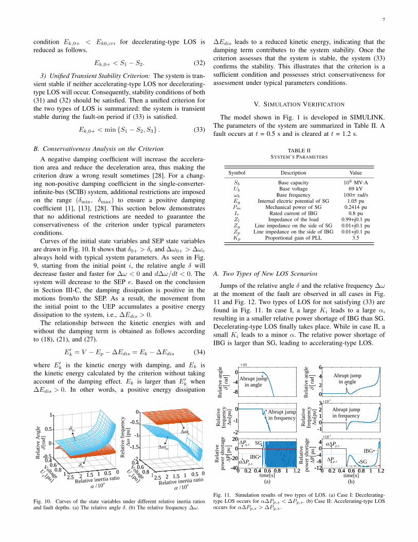
V. SIMULATION VERIFICATION
The model shown in Fig. 1 is developed in SIMULINK.The parameters of the system are summarized in Table II. Afault occurs at t = 0.5 s and is cleared at t = 1.2 s.
TABLE IISYSTEM’S PARAMETERS
Symbol Description Value
Sb Base capacity 108 MV·AUb Base voltage 69 kVωb Base frequency 100π rad/sEg Internal electric potential of SG 1.05 puPm Mechanical power of SG 0.2414 puIr Rated current of IBG 0.8 puZl Impedance of the load 0.99+j0.1 puZg Line impedance on the side of SG 0.01+j0.1 puZp Line impedance on the side of IBG 0.01+j0.1 puKp Proportional gain of PLL 3.5
A. Two Types of New LOS Scenarios
Jumps of the relative angle δ and the relative frequency ∆ωat the moment of the fault are observed in all cases in Fig.11 and Fig. 12. Two types of LOS for not satisfying (33) arefound in Fig. 11. In case I, a large Ki leads to a large α,resulting in a smaller relative power shortage of IBG than SG.Decelerating-type LOS finally takes place. While in case II, asmall Ki leads to a minor α. The relative power shortage ofIBG is larger than SG, leading to accelerating-type LOS.
SG
IBG,p sP
,g sP
Abrupt jumpin frequency
Abrupt jumpin angle
Abrupt jumpin frequency
SG
IBG,p sP
,g sP
Abrupt jumpin angle
Rel
ativ
efr
equen
cyΔω
[pu]
Rel
ativ
ep
ow
er s
ho
rtag
eP
pu
R
elat
ive
angle
rad
Rel
ativ
efr
equen
cyΔω
[pu]
Rel
ativ
ep
ow
er s
ho
rtag
eP
pu
R
elat
ive
angle
rad
0 0.2 0.4 0.6 0.8 1 1.20 0.2 0.4 0.6 0.8 1 1.2time[s]
(a)
-40
-20
0
20
-40
-20
0
20
-8
-4
0
-8
-4
0
-2
-1
0
-2
-1
0
0
2
4
6
0
2
4
6
time[s](b)
×10-1
×10-1
-1
0
1
2
3
-1
0
1
2
3
-12
-8
-4
0
4
-12
-8
-4
0
4
×10
0 0.2 0.4 0.6 0.8 1 1.20 0.2 0.4 0.6 0.8 1 1.2
Fig. 11. Simulation results of two types of LOS. (a) Case I: Decelerating-type LOS occurs for α∆Pp,s < ∆Pg,s. (b) Case II: Accelerating-type LOSoccurs for α∆Pp,s > ∆Pg,s.

8
SG
IBG
Abrupt jumpin frequency
0 0.2 0.4 0.6 0.8 1 1.20 0.2 0.4 0.6 0.8 1 1.2
Abrupt jumpin angle Abrupt jump
in angle
Abrupt jumpin frequencyR
elat
ive
freq
uen
cyΔω
[pu]
Rel
ativ
ep
ow
er s
ho
rtag
eP
pu
R
elat
ive
angle
rad
SG
IBG
Rel
ativ
efr
equen
cyΔω
[pu]
Rel
ativ
ep
ow
er s
ho
rtag
eP
pu
R
elat
ive
angle
rad
-3
-2
-1
0
-3
-2
-1
0
SG
IBG
0
2
4
6
0
2
4
6
×10-1
×10-1
-12
-8
-4
0
4
-12
-8
-4
0
4
-1
0
1
2
3
-1
0
1
2
3
time[s](a)
time[s](a)
time[s](b)
time[s](b)
time[s](c)
time[s](c)
time[s](d)
time[s](d)
-1
0
1
-1
0
1
-2
-1
0
1
-2
-1
0
1
-4048
1216
-4048
1216
-12
-8
-4
0
-12
-8
-4
0
-16-12-8-40
-16-12-8-40
0
4
8
12
0
4
8
12
-16-12-8-40
-16-12-8-40
×10-1
×10-1×10⁻²
-4
-2
0
2
-4
-2
0
2
Rel
ativ
ep
ow
er s
ho
rtag
eP
pu
Rel
ativ
efr
equen
cyΔω
[pu]
Rel
ativ
e an
gle
rad
×10-1
×10-1
SG
IBG
Abrupt jumpin frequency
Abrupt jumpin angle
,p sP
,g sP
0 0.2 0.4 0.6 0.8 1 1.20 0.2 0.4 0.6 0.8 1 1.20 0.2 0.4 0.6 0.8 1 1.20 0.2 0.4 0.6 0.8 1 1.20 0.2 0.4 0.6 0.8 1 1.20 0.2 0.4 0.6 0.8 1 1.2
Rel
ativ
e an
gle
rad
Rel
ativ
efr
equen
cyΔω
[pu]
Rel
ativ
ep
ow
er s
ho
rtag
eP
pu
Abrupt jump
in angle
Abrupt jumpin frequency
Fig. 12. Simulation results with different parameters. (a) Case II: The system is unstable when Ki = 40, Tg = 0.8 pu and Rf = 0.1 Ω. (b) Case III: Thesystem becomes stable when Ki is adjusted to 200. (c) Case IV: The system becomes stable when Tg increases to 2 pu. (d) Case V: The system becomesstable when the fault is less severe and Rf increases to 3 Ω.
B. Influence of Parameters
Adjusting the parameters of case II, the system becomesstable in cases III-V as shown in Fig. 12 (b)-(d). In case II,the relative power shortage of the IBG is larger than that ofthe SG. The integral gain Ki of the PLL is increased in caseIII to get a larger α, thus changing the extreme imbalancebetween the relative power shortage of IBG and SG. δ doesnot exceed the UEPs on the left and right sides, then the systemremains stable. In case IV, α increases with a larger inertia ofSG, also leading to a stable system. An intuitive explanationfor the stability phenomenon is that the frequency of the SGdecreases slower with a larger inertia, and the IBG can keepup with the changes. In case V, the fault becomes less severe.The redistribution of the power mitigates the relative powershortage of SG and alleviates the serious mismatch betweenthe shortages of IBG and SG, so as to stabilize the systemstability.
As shown in Table III, to enhance the transient stabilityof the system, integral gain Ki should be chosen adaptivelyto adjust the inertia of the IBG to meet different operationconditions.
C. Effectiveness of the Criterion
The results of the criterion assessment and the simulationare shown in Table III. The criterion results are consistent withthe simulation results in cases I-III. The stability/instability ofthe system and the type of instability are effectively evaluated.The criterion is proved to be an effective method for transientstability assessment of the IBG-SG system.
VI. CONCLUSION
Transient stability of low-inertia power systems with IBGis analytically studied in this paper. A hybrid IBG-SG sys-tem is established to characterize the interactions betweenelectromagnetic dynamics of the IBG and electromechanicaldynamics of the SG in the low-inertia grid under fault. A delta-power-frequency model is developed to describe the transientbehavior of the IBG-SG system. Based on the model, newmechanisms are revealed from the energy perspective. Thefirst is that two new types of LOS, accelerating-type LOS anddecelerating-type LOS, are clarified, depending on the relativepower imbalance of the IBG and the SG. And a good matchbetween the inertia of the IBG and the SG helps to balance thepowers and stabilize the system. The second is that the relativeangle and frequency abruptly jump at the moment of a fault,affecting the energy of the system. The third is that the cosinedamping coefficient is induced by the IBG. The damping isproved to have a beneficial effect on the transient stability byintroducing a positive energy dissipation. A unified criterionfor both two types of LOS is adopted to evaluate the stabilityusing the energy function method. The conservativeness of thecriterion is ensured in addressing the effect of the jumps andthe damping term. Simulations verify the correctness of theanalysis and the effectiveness of the criterion.
Other dynamic loops such as the DC voltage control loop,the fast frequency support, and the stability during the faultrecovery period are beyond the scope of this paper, which willbe our future work.
TABLE IIIRESULTS OF THE CRITERION AND THE SIMULATION
Case Ki Tg Rf Conditions Criterion Result Simulation ResultI 1500 0.8 pu 0.1 Ω a < 0, Ek,0+ > S1 − S2 Decelerating-type LOS Decelerating-type LOSII 44 0.8 pu 0.1 Ω a > 0, Ek,0+ > S3 Accelerating-type LOS Accelerating-type LOSIII 200 0.8 pu 0.1 Ω a < 0, Ek,0+ < S1 − S2 Stable Stable

9
REFERENCES
[1] X. He, H. Geng, R. Li, and B. C. Pal, “Transient stability analysisand enhancement of renewable energy conversion system during LVRT,”IEEE Trans. Sustain. Energy, vol. 11, no. 3, pp. 1612–1623, Jul. 2020.
[2] Z. Shuai, C. Shen, X. Liu, Z. Li, and Z. J. Shen, “Transient angle stabilityof virtual synchronous generators using Lyapunov’s direct method,”IEEE Trans. Smart Grid, vol. 10, no. 4, pp. 4648–4661, Jul. 2019.
[3] X. He, H. Geng, and G. Mu, “Modeling of wind turbine generators forpower system stability studies: A review,” Renew. Sust. Energ. Rev., vol.143, p. 110865, Jun. 2021.
[4] S. Khazaee, M. Hayerikhiyavi, and S. Montaser Kouhsari, “A direct-based method for real-time transient stability assessment of powersystems,” Comput. Res. Prog. Appl. Sci. and Eng. (CRPASE), vol. 6,no. 2, pp. 108–113, Jun. 2020.
[5] Y. Xue, T. Van Cutsem, and M. Ribbens-Pavella, “A simple directmethod for fast transient stability assessment of large power systems,”IEEE Trans. Power Syst., vol. 3, no. 2, pp. 400–412, May. 1988.
[6] Y. Xue and M. Pavella, “Extended equal-area criterion: an analyticalultra-fast method for transient stability assessment and preventive controlof power systems,” Int. J. Electr. Power Energy Syst., vol. 11, no. 2, pp.131–149, Apr. 1989.
[7] Y. Xue, T. Van Custem, and M. Ribbens-Pavella, “Extended equal areacriterion justifications, generalizations, applications,” IEEE Trans. PowerSyst., vol. 4, no. 1, pp. 44–52, Feb. 1989.
[8] X. He and H. Geng, “Transient stability of power systems integrated withinverter-based generation,” IEEE Trans. Power Syst., vol. 36, no. 1, pp.553–556, Jan. 2021.
[9] B. Kroposki, B. Johnson, Y. Zhang, V. Gevorgian, P. Denholm, B.-M.Hodge, and B. Hannegan, “Achieving a 100% renewable grid: Operatingelectric power systems with extremely high levels of variable renewableenergy,” IEEE Power Energy Mag., vol. 15, no. 2, pp. 61–73, Mar. 2017.
[10] T. Ji, T. Wang, S. Huang, and M. Jin, “Comparative analysis ofsynchronization stability domain for power systems integrated withPMSG based on the direct method,” in Proc. 4th Inte. Conf. Energy,Electr. Power Eng. (CEEPE), Apr. 2021, pp. 547–551.
[11] X. Wang, M. G. Taul, H. Wu, Y. Liao, F. Blaabjerg, and L. Harne-fors, “Grid-synchronization stability of converter-based resources—Anoverview,” IEEE Open J. Ind. Appl., vol. 1, pp. 115–134, Aug. 2020.
[12] Q. Hu, L. Fu, F. Ma, and F. Ji, “Large signal synchronizing instabilityof PLL-based VSC connected to weak AC grid,” IEEE Trans. PowerSyst., vol. 34, no. 4, pp. 3220–3229, Jul. 2019.
[13] X. He, H. Geng, J. Xi, and J. M. Guerrero, “Resynchronization analysisand improvement of grid-connected VSCs during grid faults,” IEEETrans. Sustain. Energy, vol. 9, no. 1, pp. 438–450, Nov. 2019.
[14] Q. Hu, J. Hu, H. Yuan, H. Tang, and Y. Li, “Synchronizing stabilityof DFIG-based wind turbines attached to weak AC grid,” in Proc. 17thInte. Conf. Electr. Mach. Syst. (ICEMS), Oct. 2014, pp. 2618–2624.
[15] M. G. Taul, X. Wang, P. Davari, and F. Blaabjerg, “An overviewof assessment methods for synchronization stability of grid-connectedconverters under severe symmetrical grid faults,” IEEE Trans. PowerElectron., vol. 34, no. 10, pp. 9655–9670, Oct. 2019.
[16] H. Wu and X. Wang, “Design-oriented transient stability analysisof PLL-synchronized voltage-source converters,” IEEE Trans. PowerElectron., vol. 35, no. 4, pp. 3573–3589, Apr. 2020.
[17] X. He, S. Pan, and H. Geng, “Transient stability of hybrid power systemsdominated by different types of grid-forming devices,” IEEE Trans.Energy Convers., 2021, in press.
[18] Q. Hu, L. Fu, F. Ma, F. Ji, and Y. Zhang, “Analogized synchronous-generator model of PLL-based VSC and transient synchronizing stabilityof converter dominated power system,” IEEE Trans. Sustain. Energy,vol. 12, no. 2, pp. 1174–1185, Apr. 2021.
[19] M. Zarifakis, W. T. Coffey, Y. P. Kalmykov, and S. V. Titov, “Modelsfor the transient stability of conventional power generating stationsconnected to low inertia systems,” Eur. Phys. J. Plus, vol. 132, no. 6,pp. 1–13, Jun. 2017.
[20] S. Ma, H. Geng, L. Liu, G. Yang, and B. C. Pal, “Grid-synchronizationstability improvement of large scale wind farm during severe grid fault,”IEEE Trans. Power Syst., vol. 33, no. 1, pp. 216–226, Jan. 2018.
[21] X. He, H. Geng, and S. Ma, “Transient stability analysis of grid-tiedconverters considering PLL’s nonlinearity,” CPSS Trans. Power Electron.Appl., vol. 4, no. 1, pp. 40–49, Mar. 2019.
[22] F. Milano, F. Dorfler, G. Hug, D. J. Hill, and G. Verbic, “Foundationsand challenges of low-inertia systems (invited paper),” in Proc. PowerSyst. Comput. Conf. (PSCC), Jun. 2018, pp. 1–25.
[23] O. Goksu, R. Teodorescu, C. L. Bak, F. Iov, and P. C. Kjær, “Instabilityof wind turbine converters during current injection to low voltage gridfaults and PLL frequency based stability solution,” IEEE Trans. PowerSyst., vol. 29, no. 4, pp. 1683–1691, Jul. 2014.
[24] H. Geng, L. Liu, and R. Li, “Synchronization and reactive currentsupport of PMSG-based wind farm during severe grid fault,” IEEE Trans.Sustain. Energy, vol. 9, no. 4, pp. 1596–1604, Oct. 2018.
[25] U. Markovic, J. Vorwerk, P. Aristidou, and G. Hug, “Stability analysisof converter control modes in low-inertia power systems,” in Proc. IEEEPES Innov. Smart Grid Technol. Conf. Eur. (ISGT-Europe), Oct. 2018,pp. 1–6.
[26] Y.-H. Moon, B.-K. Choi, and T.-H. Roh, “Estimating the domain ofattraction for power systems via a group of damping-reflected energyfunctions,” Automatica, vol. 36, no. 3, pp. 419–425, Mar. 2000.
[27] A. Michel, A. Fouad, and V. Vittal, “Power system transient stabilityusing individual machine energy functions,” IEEE Trans. Circuits Syst.,vol. 30, no. 5, pp. 266–276, May. 1983.
[28] X. Fu, J. Sun, M. Huang, Z. Tian, H. Yan, H. H.-C. Iu, P. Hu, and X. Zha,“Large-signal stability of grid-forming and grid-following controls involtage source converter: A comparative study,” IEEE Trans. PowerElectron., vol. 36, no. 7, pp. 7832–7840, Jul. 2021.