1

Transforming Probabilitieswith Combinational Logic

Weikang Qian, Marc D. Riedel, Hongchao Zhou, and Jehoshua Bruck

Abstract—Schemes for probabilistic computation can exploitphysical sources to generate random values in the form of bitstreams. Generally, each source has a fixed bias and so providesbits that have a specific probability of being one versus zero. Ifmany different probability values are required, it can be difficultor expensive to generate all of these directly from physicalsources. In this work, we demonstrate novel techniques forsynthesizing combinational logic that transforms a set of sourceprobabilities into different target probabilities. We consider threedifferent scenarios in terms of whether the source probabilitiesare specified and whether they can be duplicated. In the case thatthe source probabilities are not specified and can be duplicated,we provide a specific choice, the set {0.4, 0.5}; we show howto synthesize logic that transforms probabilities from this setinto arbitrary decimal probabilities. Further, we show that forany integer n ≥ 2, we can find a single source probability thatcan be transformed into arbitrary base-n fractional probabilitiesof the form m

nd . In the case that the source probabilities arespecified and cannot be duplicated, we provide two methods forsynthesizing logic to transform them into target probabilities. Inthe case that the source probabilities are not specified, but oncechosen cannot be duplicated, we provide an optimal choice.

Index Terms—logic synthesis, combinational logic, probabilisticlogic, probabilistic signals, random bit streams, stochastic bitstreams

I. INTRODUCTION AND BACKGROUND

Most digital circuits are designed to map deterministicinputs of zero and one to deterministic outputs of zero andone. An alternative paradigm is to design circuits that operateon stochastic bit streams. Each stream represents a real-valuednumber x (0 ≤ x ≤ 1) through a sequence of random bitsthat have probability x of being one and probability 1 − xof being zero. Such circuits can be viewed as constructs thataccept real-valued probabilities as inputs and compute real-valued probabilities as outputs.

Consider the example shown in Figure 1. Given independentstochastic bit streams as inputs, an AND gate performs mul-tiplication: it produces an output bit stream with a probabilitythat is the product of the probabilities of the input bit streams.In prior work, we proposed a general method for synthesizingarbitrary functions through logical computation on stochasticbit streams [1], [2].

Stochastic bit streams can be generated with pseudo-randomconstructs, such as linear feedback shift registers. Alterna-tively, if physical sources of randomness are available, these

This work is supported by a grant from the Semiconductor ResearchCorporation’s Focus Center Research Program on Functional EngineeredNano-Architectonics, contract No. 2003-NT-1107, as well as a CAREERAward, #0845650, from the National Science Foundation.

Weikang Qian and Marc Riedel are with the Department of Electrical andComputer Engineering, University of Minnesota, Minneapolis, MN 55455,USA. Email: {qianx030, mriedel}@umn.edu.

Hongchao Zhou and Jehoshua Bruck are with the Department of ElectricalEngineering, California Institute of Technology, Pasadena, CA 91125, USA.Email: {hzhou, bruck}@caltech.edu.

AND

P(a = 1) = 0.8

P(b = 1) = 0.5

a

bc

P(c = 1) = 0.4

1,1,0,1,1,1,1,1,0,1

1,0,1,1,0,0,1,0,0,1

1,0,0,1,0,0,1,0,0,1

Fig. 1: An AND gate multiplies the probabilities of stochastic bitstreams. Here the input streams have probabilities 0.8 and 0.5. Theprobability of the output stream is 0.8× 0.5 = 0.4.

could be used directly. For example, in [3], the authorspropose a so-called probabilistic CMOS (PCMOS) constructthat generates random bits from intrinsic sources of noise.In [4], PCMOS switches are applied to form a probabilisticsystem-on-a-chip (PSOC); this system provides intrinsic ran-domness to the application layer, so that it can be exploitedby probabilistic algorithms.

For schemes that generate stochastic bit streams from phys-ical sources, a significant limitation is the cost of generatingdifferent probability values. For instance, if each probabilityvalue is determined by a specific voltage level, different volt-age levels are required to generate different probability values.For an application that requires many different values, manyvoltage regulators are required; this might be prohibitivelycostly in terms of area as well as energy.

This paper presents a synthesis strategy to mitigate thisissue: we describe a method for transforming a set of sourceprobabilities into different target probabilities entirely throughcombinational logic. For what follows, when we say “withprobability p,” we mean “with a probability p of being at log-ical one.” When we say “a circuit,” we mean a combinationalcircuit built with logic gates.

Example 1Suppose that we have a set of source probabilities S ={0.4, 0.5}. As illustrated in Figure 2, we can transform this setinto new probabilities:

1) Given an input x with probability 0.4, an inverter will havean output z with probability 0.6 since

P (z = 1) = P (x = 0) = 1− P (x = 1). (1)

2) Given inputs x and y with independent probabilities 0.4and 0.5, an AND gate will have an output z with probabil-ity 0.2 since

P (z = 1) = P (x = 1, y = 1)= P (x = 1)P (y = 1).

(2)

3) Given inputs x and y with independent probabilities 0.4and 0.5, a NOR gate will have an output z with probability

2

P(x = 1) = 0.4x z

P(z = 1) = 0.6

(a)

AND

P(x = 1) = 0.4

P(y = 1) = 0.5

x

yz

P(z = 1) = 0.2

(b)

NOR

P(x = 1) = 0.4

P(y = 1) = 0.5

x

yz

P(z = 1) = 0.3

(c)

Fig. 2: An illustration of transforming a set of source probabilitiesinto new probabilities with logic gates. (a): An inverter implementingpz = 1− px. (b): An AND gate implementing pz = px · py . (c): ANOR gate implementing pz = (1− px) · (1− py).

0.3 sinceP (z = 1) = P (x = 0, y = 0) = P (x = 0)P (y = 0)

= (1− P (x = 1))(1− P (y = 1)).

Thus, using combinational logic, we obtain the set of probabil-ities {0.2, 0.3, 0.6} from the set {0.4, 0.5}. �

Motivated by this example, we consider the problem of howto synthesize combinational logic to transform a set of sourceprobabilities S = {p1, p2, . . . , pn} into a target probability q.We assume that the probabilistic sources are all independent.We consider three scenarios:

1) Scenario One: Consider the situation in which we havethe flexibility to choose the probabilities produced byphysical sources, say by setting them with specific voltagevalues. We can produce multiple independent copies ofeach probability cheaply, since each copy uses the samevoltage level. However, generating different probabilitiesis costly, since this entails generating different voltagelevels. Here we seek to minimize the size of the sourceset of probabilities S, assuming that each probability inS can be used an arbitrary number of times. (We saythat the probability can be duplicated.) The problem is tofind a small set S and to demonstrate how to synthesizelogic that transforms values from this set into an arbitrarytarget probability q.

2) Scenario Two: Consider the situation in which there isno flexibility with the random sources; these produce afixed set of probabilities S. The set S can be a multiset,i.e., one that could contain multiple elements of the samevalue. However, we cannot duplicate the probabilities; wehave to work with what is given to us. The problem ishow to synthesize logic that has input probabilities takenfrom S and produces an output probability q, where eachelement in S can be used as an input probability at mostonce.

3) Scenario Three: Consider the situation in which wehave the flexibility to choose the probabilities but thevalues we choose cannot be duplicated cheaply; it costsas much to generate each copy as any other value. This

situation occurs if we use pseudo-random constructs suchas linear feedback shift registers: the cost of each pseudo-random bit stream is the same no matter what probabilityvalue is realized. Suppose that we establish a budgetof n random or pseudo-random sources. The problemis to find a set S of n probabilities such that we cansynthesize logic that transforms values from this set intoan arbitrary probability q. Here the elements of S cannotbe duplicated; again, S can be a multiset.

To summarize, we consider scenarios that differ in respect to:1) Whether the set S is specified or not.2) Whether the probabilities from S can be duplicated or

not.Our contributions are:

1) For Scenario One, we demonstrate that a particular setconsisting of only two elements, S = {0.4, 0.5}, can betransformed into arbitrary decimal probabilities. Further,we propose an algorithm based on fraction factorizationto optimize the depth of the resulting circuit. Figure 3shows a circuit synthesized by our algorithm to realize thedecimal output probability 0.119 from the input probabil-ities 0.4 and 0.5. The circuit consists of AND gates andinverters: each AND gate performs a multiplication of itsinputs and each inverter performs a one-minus operationof its input.

AND

AND

AND

AND

AND

AND

0.40.6

0.5

0.30.7

0.4

0.50.2

0.14

0.5

0.5

0.40.6

0.3

0.15

0.85

0.119

Fig. 3: A circuit synthesized by our algorithm to realize the decimaloutput probability 0.119 from the input probabilities 0.4 and 0.5.

2) Also for Scenario One, we prove that for any giveninteger n ≥ 2, there exists a set S consisting of a singleelement that can be transformed into arbitrary base-nfractional probabilities of the form m

nd .3) For Scenario Two, we solve the problem by transforming

it into a linear 0-1 programming problem. Althoughapproximate, the solution is optimal in terms of thedifference between the target probability and the actualoutput probability.

4) Also for Scenario Two, we provide a greedy algorithm.Although the solution that it yields is not optimal, thedifference between the target probability and the actualoutput probability is bounded. The algorithm runs veryefficiently, yielding a solution in O(n2) time, where n isthe cardinality of the set S.

5) For Scenario Three, we provide an optimal choice of theset S. Specifically, we first define a quality measure H(S)for each choice S consisting of arbitrary probabilities. Weprove that if the cardinality of S is n, then a lower bound

on H(S) is1

4(22n − 1). Then we show that the set of

source probabilities

S = {p|p =22k

22k + 1, k = 0, 1, . . . , n− 1}

3

achieves the lower bound.

II. RELATED WORK

The task of analyzing circuits operating on probabilistic in-puts is well understood [5]. Aspects such as signal correlationsof reconvergent paths must be taken into account. Algorithmicdetails for such analysis were first fleshed out by the testingcommunity [6]. They have also found mainstream applicationfor tasks such as timing and power analysis [7], [8].

The problem of synthesizing circuits to transform a givenset of probabilities into a new set of probabilities appearsin an early set of papers by Gill [9], [10]. He focused onsynthesizing sequential state machines for this task.

Motivated by problems in neural computation, Jeavons etal. considered the problem of transforming stochastic binarysequences through what they call “local algorithms:” fixedfunctions applied to concurrent bits in different sequences [11].This is equivalent to performing operations on stochastic bitstreams with combinational logic, so in essence they wereconsidering the same problem as we are. Their main result wasa method for generating binary sequences with probability m

nd

from a set of stochastic binary sequences with probabilities inthe set { 1

n , 2n , . . . , n−1

n }. This is equivalent to our Theorem 2.In contrast to the work of Jeavons et al., our primary focus ison minimizing the number of source probabilities needed torealize arbitrary base-n fractional probabilities.

The proponents of PCMOS discussed the problem of syn-thesizing combinational logic to transform probability val-ues [4]. These authors suggested using a tree-based circuitto realize a set of target probabilities. This was positioned asfuture work; no details were given.

Wilhelm and Bruck proposed a general framework forsynthesizing switching circuits to achieve a desired proba-bility [12]. Switching circuits were originally discussed byShannon [13]. These consist of relays that are either openor closed; the circuit computes a logical value of one ifthere exists a closed path through the circuit. Wilhelm andBruck considered stochastic switching circuits, in which eachswitch has a certain probability of being open or closed. Theyproposed an algorithm that generates the requisite stochasticswitching circuit to compute any binary probability.

Zhou and Bruck generalized Wilhelm and Bruck’swork [14]. They considered the problem of synthesizinga stochastic switching circuit to realize an arbitrary base-n fractional probability m

nd from a probabilistic switch set{ 1

n , 2n , . . . , n−1

n }. They showed that when n is a multipleof 2 or 3, such a realization is possible. However, for anyprime number n greater than 3, there exists a base-n fractionalprobability that cannot be realized by any stochastic switchingcircuit.

In contrast to the work of Gill, to that of Wilhelm andBruck, and to that of Zhou and Bruck, we consider combina-tional circuits: memoryless circuits consisting of logic gates.Our approach dovetails nicely with the circuit-level PCMOSconstructs. It is orthogonal to the switch-based approach ofZhou and Bruck. Note that Zhou and Bruck assume that theprobabilities in the given set S can be duplicated. We alsoconsider the case where they cannot.

III. SCENARIO ONE: SET S IS NOT SPECIFIED AND THEELEMENTS CAN BE DUPLICATED

In this scenario, we assume that the set S of probabilities isnot specified. Once the set has been determined, each elementof the set can be used as an input probability an arbitrarynumber of times. The inputs are all assumed to be independent.As discussed in the introduction, we seek a set S of small size.

A. Generating Decimal ProbabilitiesIn this section, we consider the case where the target

probabilities are represented as decimal numbers. The problemis to find a small set S of source probabilities that can betransformed into an arbitrary target decimal probability. Weprovide a set S consisting of two elements.

Theorem 1With circuits consisting of fanin-two AND gates and inverters,we can transform the set of source probabilities {0.4, 0.5} intoan arbitrary decimal probability. �

Proof: First, we note that an inverter with a probabilisticinput gives an output probability equal to one minus the inputprobability, as was shown in Equation (1). An AND gate withtwo independent inputs performs a multiplication of the inputprobabilities, as was shown in Equation (2). Thus, we needto prove: with the two operations 1 − x and x · y, we cantransform the values from the set {0.4, 0.5} into arbitrarydecimal fractions. We prove this statement by induction onthe number of digits n after the decimal point.

Base case:1) n = 0. The values 0 and 1 correspond to deterministic

inputs of zero and one, respectively.2) n = 1. We can generate 0.1, 0.2, and 0.3 as follows:

0.1 = 0.4× 0.5× 0.5,

0.2 = 0.4× 0.5,

0.3 = (1− 0.4)× 0.5.

Since we can generate the decimal fractions 0.1, 0.2, 0.3,and 0.4, we can generate 0.6, 0.7, 0.8, and 0.9 with anextra 1−x operation. Together with the source value 0.5,we can transform the pair of values 0.4 and 0.5 into anydecimal fraction with one digit after the decimal point.

Inductive step:Assume that the statement holds for all m ≤ (n−1). Consideran arbitrary decimal fraction z with n digits after the decimalpoint. Let u = 10n · z. Here u is an integer.

Consider the following four cases.1) The case where 0 ≤ z ≤ 0.2.

a) The integer u is divisible by 2. Let w = 5z. Then0 ≤ w ≤ 1 and w = (u/2) · 10−n+1, having at most(n− 1) digits after the decimal point. Thus, based onthe induction hypothesis, we can generate w. It followsthat z can be generated as z = 0.4× 0.5× w.

b) The integer u is not divisible by 2 and 0 ≤ z ≤ 0.1. Letw = 10z. Then 0 ≤ w ≤ 1 and w = u·10−n+1, havingat most (n − 1) digits after the decimal point. Thus,based on the induction hypothesis, we can generate w.It follows that z can be generated as z = 0.4× 0.5×0.5× w.

4

c) The integer u is not divisible by 2 and 0.1 < z ≤ 0.2.Let w = 2 − 10z. Then 0 ≤ w < 1 and w = 2 −u · 10−n+1, having at most (n − 1) digits after thedecimal point. Thus, based on the induction hypothesis,we can generate w. It follows that z can be generatedas z = (1− 0.5× w)× 0.4× 0.5.

2) The case where 0.2 < z ≤ 0.4.a) The integer u is divisible by 4. Let w = 2.5z. Then

0 < w ≤ 1 and w = (u/4) · 10−n+1, having at most(n− 1) digits after the decimal point. Thus, based onthe induction hypothesis, we can generate w. It followsthat z can be generated as z = 0.4× w.

b) The integer u is not divisible by 4 but is divisible by 2.Let w = 2 − 5z. Then 0 ≤ w < 1 and w = 2 −(u/2) · 10−n+1, having at most (n− 1) digits after thedecimal point. Thus, based on the induction hypothesis,we can generate w. It follows that z can be generatedas z = (1− 0.5× w)× 0.4.

c) The integer u is not divisible by 2 and 0.2 < u ≤ 0.3.Let w = 10z − 2. Then 0 < w ≤ 1 and w = u ·10−n+1 − 2, having at most (n − 1) digits after thedecimal point. Thus, based on the induction hypothesis,we can generate w. It follows that z can be generatedas z = (1− (1− 0.5× w)× 0.5)× 0.4.

d) The integer u is not divisible by 2 and 0.3 < u ≤ 0.4.Let w = 4 − 10z. Then 0 ≤ w < 1 and w = 4 −u · 10−n+1, having at most (n − 1) digits after thedecimal point. Thus, based on the induction hypothesis,we can generate w. It follows that z can be generatedas z = (1− 0.5× 0.5× w)× 0.4.

3) The case where 0.4 < z ≤ 0.5. Let w = 1−2z. Then 0 ≤w < 0.2 and w falls into case 1. Thus, we can generatew. It follows that z can be generated as z = 0.5×(1−w).

4) The case where 0.5 < z ≤ 1. Let w = 1 − z. Then0 ≤ w < 0.5 and w falls into one of the above threecases. Thus, we can generate w. It follows that z can begenerated as z = 1− w.

For all of the above cases, we proved that we can transformthe pair of values 0.4 and 0.5 into z with the two operations1−x and x · y. Thus, we proved the statement for all m ≤ n.By induction, the statement holds for all integers n.

Based on the proof above, we derive an algorithm tosynthesize a circuit that transforms the probabilities from theset {0.4, 0.5} into an arbitrary decimal probability z. This isshown in Algorithm 1.

Algorithm 1 Synthesize a circuit consisting of AND gates andinverters that transforms the probabilities from the set {0.4, 0.5} intoa target decimal probability.

1: {Given an arbitrary decimal probability 0 ≤ z ≤ 1.}2: Initialize ckt;3: while GetDigits(z) > 1 do4: (ckt, z)⇐ ReduceDigit(ckt, z);5: ckt⇐ AddBaseCkt(ckt, z); {Base case: z has at most one digit

after the decimal point.}6: return ckt;

The function GetDigits(z) in Algorithm 1 returns the num-ber of digits after the decimal point of z. The algorithm iteratesuntil z has at most one digit after the decimal point. Duringeach iteration, it calls the function ReduceDigit(ckt, z). Thisfunction, shown in Algorithm 2, converts z into a number w

with one less digit after the decimal point than z. It is imple-mented based on the inductive step in the proof of Theorem 1.Finally, the algorithm calls the function AddBaseCkt(ckt, z)to add logic gates to realize a number z with at most one digitafter the decimal point; this corresponds to the base case ofthe proof.

Algorithm 2 ReduceDigit(ckt, z)

1: {Given a partial circuit ckt and an arbitrary decimal probability0 ≤ z ≤ 1.}

2: n⇐ GetDigits(z);3: if z > 0.5 then {Case 4}4: z ⇐ 1− z; AddInverter(ckt);5: if 0.4 < z ≤ 0.5 then {Case 3}6: z ⇐ z/0.5; AddAND(ckt, 0.5);7: z ⇐ 1− z; AddInverter(ckt);8: if z ≤ 0.2 then {Case 1}9: z ⇐ z/0.4; AddAND(ckt, 0.4);

10: z ⇐ z/0.5; AddAND(ckt, 0.5);11: if GetDigits(z) < n then12: go to END;13: if z > 0.5 then14: z ⇐ 1− z; AddInverter(ckt);15: z = z/0.5; AddAND(ckt, 0.5);16: else {Case 2: 0.2 < z ≤ 0.4}17: z ⇐ z/0.4; AddAND(ckt, 0.4);18: if GetDigits(z) < n then19: go to END;20: z ⇐ 1− z; AddInverter(ckt);21: z ⇐ z/0.5; AddAND(ckt, 0.5);22: if GetDigits(z) < n then23: go to END;24: if z > 0.5 then25: z ⇐ 1− z; AddInverter(ckt);26: z = z/0.5; AddAND(ckt, 0.5);27: END: return ckt, z;

The function ReduceDigit(ckt, z) in Algorithm 2 buildsthe circuit from the output back to the inputs. During itsconstruction, the circuit always has a single dangling input.Initially, the circuit is just a wire connecting an input to theoutput. The function AddInverter(ckt) attaches an inverterto the dangling input creating a new dangling input. Thefunction AddAND(ckt, p) attaches a fanin-two AND gate tothe dangling input; one of the AND gate’s inputs is thenew dangling input; the other is set to a random source ofprobability p. In Algorithm 2, Lines 3–4 correspond to Case4 in the proof; Lines 5–7 correspond to Case 3; Lines 8–15correspond to Case 1; and Lines 16–26 correspond to Case 2.

The area complexity of the synthesized circuit is linear inthe number of digits after the target value’s decimal point,since at most 3 AND gates and 3 inverters are needed togenerate a value with n digits after the decimal point from avalue with (n−1) digits after the decimal point.1 The numberof AND gates in the synthesized circuit is at most 3n.

Example 2We show how to generate the probability value 0.757. Basedon Algorithm 1, we can derive a sequence of operations that

1In Case 3, z is transformed into w = 1− 2z where w falls in Case 1(a).Thus, we actually need only 3 AND gates and 1 inverter for Case 3. For theother cases, it is not hard to see that we need at most 3 AND gates and 3inverters.

5

transform 0.757 to 0.7:

0.757 1−=⇒ 0.243/0.4=⇒ 0.6075 1−=⇒ 0.3925

/0.5=⇒ 0.785

1−=⇒ 0.215/0.5=⇒ 0.43,

0.43/0.5=⇒ 0.86 1−=⇒ 0.14

/0.4=⇒ 0.35

/0.5=⇒ 0.7.

Since 0.7 can be realized as 0.7 = 1−(1−0.4)×0.5, we obtainthe circuit shown in Figure 4. (Note that here we use a black dotto represent an inverter.) �

0.4

0.5

0.60.7

0.5

0.35

0.4

0.86

0.5

0.5

0.430.785

0.6075

0.50.4

0.757

AND

ANDAND

ANDAND

ANDAND

Fig. 4: A circuit transforming the set of source probabilities{0.4, 0.5} into a decimal output probability of 0.757.

Remarks: One may question the usefulness of synthesizinga circuit that generates arbitrary decimal fractions. Wilhelmand Bruck proposed a scheme for synthesizing switchingcircuits that generate arbitrary binary probabilities [12]. Bymapping every switch connected in series to an AND gateand every switch connected in parallel to an OR gate, wecan easily derive a combinational circuit that generates anarbitrary binary probability. Since any decimal fractional valuecan be approximated by a binary fractional value, we can buildcombinational circuits implementing decimal probabilities thisway. However, the circuits synthesized by our procedure areless costly in terms of area.

To see this, consider a decimal fraction q with n digits.The circuit that Algorithm 1 synthesizes to generate q hasat most 3n AND gates. For the approximation error of thebinary fraction for q to be below 1/10n, the number of digitsm of the binary fraction should be greater than n log2 10.In [12], it is proved that the minimal number of probabilisticswitches needed to generate a binary fraction of m digitsis m. Assuming that we build an equivalent combinationalcircuit consisting of AND gates and inverters, we need m− 1AND gates to implement the binary fraction.2 Thus, thecombinational logic realizing the binary approximation needsmore than n log2 10 ≈ 3.32n AND gates. This is more thanthe number of AND gates in the circuit synthesized by ourprocedure.

B. Reducing the DepthThe circuits produced by Algorithm 1 have a linear topology

(i.e., each gate adds to the depth of the circuit). For practicalpurposes, we want circuits with shallower depth. In thissection, we explore two kinds of optimizations for reducingthe depth.

The first kind of optimization is at the logic level. The circuitsynthesized by Algorithm 1 is composed of inverters and

2Of course, an OR gate can be converted into an AND gate with invertersat both the inputs and the output.

ANDAND

Fanin

Cone

ab

...

(a)

AND

Fanin

Cone ...

ANDa

b

(b)

Fig. 5: An illustration of balancing to reduce the depth of the circuit.Here a and b are primary inputs. (a): The circuit before balancing.(b): The circuit after balancing.

AND gates. We can reduce its depth by properly repositioningcertain AND gates, as illustrated in Figure 5. We refer to suchoptimization as balancing.

The second kind of optimization is at a higher level, basedon the factorization of the decimal fraction. We use thefollowing example to illustrate the basic idea.

Example 3Suppose we want to generate the decimal probability value0.49.

Method based on Algorithm 1: We can derive the followingtransformation sequence:

0.49/0.5=⇒ 0.98 1−=⇒ 0.02

/0.4=⇒ 0.05

/0.5=⇒ 0.1.

The synthesized circuit is shown in Figure 6(a). Notice that thecircuit is balanced; it has five AND gates and a depth of four.3

Method based on factorization: Notice that 0.49 = 0.7 × 0.7.Thus, we can generate the probability 0.7 twice and feed thesevalues into an AND gate. The synthesized circuit is shown inFigure 6(b). Compared to the circuit in Figure 6(a), both thenumber of AND gates and the depth of the circuit are reduced.�

Algorithm 3 shows the procedure that synthesizes thecircuit based on the factorization of the decimal fraction.The factorization is actually carried out on the numerator. Acrucial function is PairCmp(al, ar, bl, br), which compares theinteger factor pair (al, ar) with the pair (bl, br) and returns apositive (negative) value if the pair (al, ar) is better (worse)than the pair (bl, br). Algorithm 4 shows how the functionPairCmp(al, ar, bl, br) is implemented.

The quality of a factor pair (al, ar) should reflect the depthof the circuit that generates the original probability basedon that factorization. For this purpose, we define a functionEstDepth(x) to estimate the depth of the circuit that generatesthe decimal fraction with a numerator x. If 1 ≤ x ≤ 9, thecorresponding fraction is x/10. EstDepth(x) is set as the depth

3When counting depth, we ignore inverters.

6

0.5

0.5

0.2

0.98

0.49

0.4

0.5

0.4

0.25

0.10.5

AND

AND

AND

AND

AND

(a)

0.49

0.5

0.5

0.4

0.40.7

0.7AND

AND

AND

(b)

Fig. 6: Synthesizing combinational logic to generate the probability0.49. (a): The circuit synthesized through Algorithm 1. (b): Thecircuit synthesized based on fraction factorization.

Algorithm 3 ProbFactor(ckt, z)

1: {Given a partial circuit ckt and an arbitrary decimal probability0 ≤ z ≤ 1.}

2: n⇐ GetDigits(z);3: if n ≤ 1 then4: ckt⇐ AddBaseCkt(ckt, z);5: return ckt;6: u⇐ 10nz; (ul, ur)⇐ (1, u); {u is the numerator of the fraction

z}7: for each factor pair (a, b) of u do8: if PairCmp(ul, ur, a, b) < 0 then9: (ul, ur)⇐ (a, b); {Choose the best factor pair for z}

10: w ⇐ 10n − u; (wl, wr)⇐ (1, w);11: for each factor pair (a, b) of w do12: if PairCmp(wl, wr, a, b) < 0 then13: (wl, wr)⇐ (a, b); {Choose the best factor pair for 1− z}14: if PairCmp(ul, ur, wl, wr) < 0 then15: (ul, ur)⇐ (wl, wr); z ⇐ w/10n;16: AddInverter(ckt);17: if IsTrivialPair(ul, ur) then {ul = 1 or ur = u}18: (ckt, z)⇐ ReduceDigit(ckt, z);19: ckt⇐ ProbFactor(ckt, z);20: return ckt;21: nl ⇐ dlog10(ul)e; nr ⇐ dlog10(ur)e;22: if nl + nr > n then {Unable to factor z into two decimal

fractions in the unit interval}23: (ckt, z)⇐ ReduceDigit(ckt, z);24: ckt⇐ ProbFactor(ckt, z);25: return ckt;26: zl ⇐ ul/10nl ; zr ⇐ ur/10nr ;27: cktl ⇐ ProbFactor(cktl, zl);28: cktr ⇐ ProbFactor(cktr, zr);29: Connect the input of ckt to an AND gate with two inputs as cktl

and cktr;30: if nl + nr < n then31: AddExtraLogic(ckt, n− nl − nr);32: return ckt;

of the circuit that generates the fraction x/10, which is

EstDepth(x) =

0, x = 4, 5, 6,

1, x = 2, 3, 7, 8,

2, x = 1, 9.

When x ≥ 10, we use a simple heuristic to estimate thedepth: we let EstDepth(x) = dlog10(x)e + 1. The intuitionbehind this is that the depth of the circuit is a monotonicallyincreasing function of the number of digits of x. The estimateddepth of the circuit that generates the original fraction based

on the factor pair (al, ar) is

max{EstDepth(al), EstDepth(ar)}+ 1. (3)

The function PairCmp(al, ar, bl, br) essentially comparesthe quality of pair (al, ar) and pair (bl, br) based on Equa-tion (3). Further details are given in Algorithm 4.

Algorithm 4 PairCmp(al, ar, bl, br)

1: {Given two integer factor pairs (al, ar) and (bl, br)}2: cl ⇐ EstDepth(al); cr ⇐ EstDepth(ar);3: dl ⇐ EstDepth(bl); dr ⇐ EstDepth(br);4: Order(cl, cr); {Order cl and cr , so that cl ≤ cr}5: Order(dl, dr); {Order dl and dr , so that dl ≤ dr}6: if cr < dr then {The circuit w.r.t. the first pair has smaller

depth}7: return 1;8: else if cr > dr then {The circuit w.r.t. the first pair has larger

depth}9: return -1;

10: else11: if cl < dl then {The circuit w.r.t. the first pair has fewer

ANDs}12: return 1;13: else if cl > dl then {The circuit w.r.t. the first pair has more

ANDs}14: return -1;15: else16: return 0;

In Algorithm 3, Lines 2–5 correspond to the trivial fractions.If the fraction z is non-trivial, Lines 6–9 choose the best factorpair (ul, ur) of u, where u is the numerator of the fraction z.Lines 10–13 choose the best factor pair (wl, wr) of w, wherew is the numerator of the fraction 1− z. Finally, Lines 14–16choose the better factor pair of (ul, ur) and (wl, wr). Here, weconsider the factorization on both z and 1− z, since in somecases the latter might be better than the former. An exampleis z = 0.37. Note that 1 − z = 0.63 = 0.7 × 0.9; this has abetter factor pair than z itself.

After obtaining the best factor pair, we check whether wecan use it. Lines 17–20 check whether the factor pair (ul, ur)is trivial; a factor pair is considered trivial if ul = 1 orur = 1. If the best factor pair is trivial, we call the functionReduceDigit(ckt, z) in Algorithm 2 to transform z into a newvalue with one less digit after the decimal point. Then weperform factorization on the new value.

If the best factor pair is non-trivial, Lines 21–25 continueto check whether the factor pair can be transformed into twodecimal fractions in the unit interval. Let nl be the number ofdigits of the integer ul and nr be the number of digits of theinteger ur. If nl+nr > n, where n is the number of digits afterthe decimal point of z, then it is impossible to use the factorpair (ul, ur) to factorize z. For example, consider z = 0.143.Although we could factorize 143 as 11×13, we cannot use thefactor pair (11, 13) since the factorization 0.11× 1.3 and thefactorization 1.1× 0.13 both contain a fraction larger than 1;a probability value can never be larger than 1.

Finally, if it is possible to use the best factor pair, Lines 26–29 synthesize two circuits for fractions ul/10nl and ur/10nr ,respectively, and then combine these two circuits with an ANDgate. Lines 30–31 check whether n > nl + nr. If this is thecase, we have

z = u/10n = ul/10nl · ur/10nr · 0.1n−nl−nr .

7

We need to add an extra AND gate with one input prob-ability as 0.1n−nl−nr and the other input probability asul/10nl · ur/10nr . The extra logic is added through thefunction AddExtraLogic(ckt, m).

C. Empirical ValidationWe empirically validate the effectiveness of the synthesis

scheme that was presented in the previous section. For logic-level optimization, we use the “balance” command of thesynthesis tool ABC [15]. We find that it is very effective inreducing the depth of tree-style circuits.4

Table I compares the quality of the circuits generated bythree different schemes. The first scheme, called “Basic,”is based on Algorithm 1. It generates a linear-style circuit.The second scheme, called “Basic+Balance,” combines Al-gorithm 1 and the logic-level balancing algorithm. The thirdscheme, called “Factor+Balance,” combines Algorithm 3 andthe logic-level balancing algorithm. We perform experimentson a set of target decimal probabilities that have n digits afterthe decimal point and average the results. Table I shows theresults for n ranging from 2 to 12. When n ≤ 5, we synthesizecircuits for all possible decimal probabilities with n digits afterthe decimal point. When n ≥ 6, we randomly choose 100,000decimal probabilities with n digits after the decimal point asthe synthesis targets. We show the average number of ANDgates, the average depth, and the average CPU runtime.

2 4 6 8 10 120

5

10

15

20

25

30

35

n

Basic+Balance #AND

Basic+Balance Depth

Factor+Balance #AND

Factor+Balance Depth

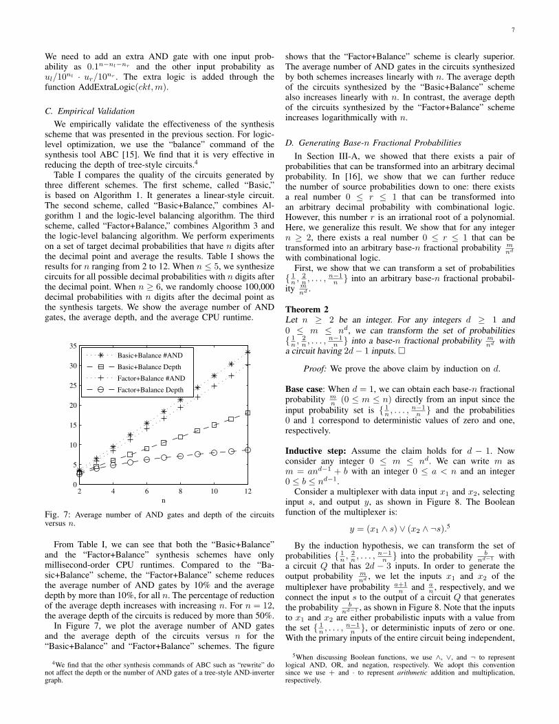
Fig. 7: Average number of AND gates and depth of the circuitsversus n.

From Table I, we can see that both the “Basic+Balance”and the “Factor+Balance” synthesis schemes have onlymillisecond-order CPU runtimes. Compared to the “Ba-sic+Balance” scheme, the “Factor+Balance” scheme reducesthe average number of AND gates by 10% and the averagedepth by more than 10%, for all n. The percentage of reductionof the average depth increases with increasing n. For n = 12,the average depth of the circuits is reduced by more than 50%.

In Figure 7, we plot the average number of AND gatesand the average depth of the circuits versus n for the“Basic+Balance” and “Factor+Balance” schemes. The figure

4We find that the other synthesis commands of ABC such as “rewrite” donot affect the depth or the number of AND gates of a tree-style AND-invertergraph.

shows that the “Factor+Balance” scheme is clearly superior.The average number of AND gates in the circuits synthesizedby both schemes increases linearly with n. The average depthof the circuits synthesized by the “Basic+Balance” schemealso increases linearly with n. In contrast, the average depthof the circuits synthesized by the “Factor+Balance” schemeincreases logarithmically with n.

D. Generating Base-n Fractional ProbabilitiesIn Section III-A, we showed that there exists a pair of

probabilities that can be transformed into an arbitrary decimalprobability. In [16], we show that we can further reducethe number of source probabilities down to one: there existsa real number 0 ≤ r ≤ 1 that can be transformed intoan arbitrary decimal probability with combinational logic.However, this number r is an irrational root of a polynomial.Here, we generalize this result. We show that for any integern ≥ 2, there exists a real number 0 ≤ r ≤ 1 that can betransformed into an arbitrary base-n fractional probability m

nd

with combinational logic.First, we show that we can transform a set of probabilities

{ 1n , 2

n , . . . , n−1n } into an arbitrary base-n fractional probabil-

ity mnd .

Theorem 2Let n ≥ 2 be an integer. For any integers d ≥ 1 and0 ≤ m ≤ nd, we can transform the set of probabilities{ 1

n , 2n , . . . , n−1

n } into a base-n fractional probability mnd with

a circuit having 2d− 1 inputs. �

Proof: We prove the above claim by induction on d.

Base case: When d = 1, we can obtain each base-n fractionalprobability m

n (0 ≤ m ≤ n) directly from an input since theinput probability set is { 1

n , . . . , n−1n } and the probabilities

0 and 1 correspond to deterministic values of zero and one,respectively.

Inductive step: Assume the claim holds for d − 1. Nowconsider any integer 0 ≤ m ≤ nd. We can write m asm = and−1 + b with an integer 0 ≤ a < n and an integer0 ≤ b ≤ nd−1.

Consider a multiplexer with data input x1 and x2, selectinginput s, and output y, as shown in Figure 8. The Booleanfunction of the multiplexer is:

y = (x1 ∧ s) ∨ (x2 ∧ ¬s).5

By the induction hypothesis, we can transform the set ofprobabilities { 1

n , 2n , . . . , n−1

n } into the probability bnd−1 with

a circuit Q that has 2d − 3 inputs. In order to generate theoutput probability m

nd , we let the inputs x1 and x2 of themultiplexer have probability a+1

n and an , respectively, and we

connect the input s to the output of a circuit Q that generatesthe probability b

nd−1 , as shown in Figure 8. Note that the inputsto x1 and x2 are either probabilistic inputs with a value fromthe set { 1

n , . . . , n−1n }, or deterministic inputs of zero or one.

With the primary inputs of the entire circuit being independent,

5When discussing Boolean functions, we use ∧, ∨, and ¬ to representlogical AND, OR, and negation, respectively. We adopt this conventionsince we use + and · to represent arithmetic addition and multiplication,respectively.

8

TABLE I: A comparison of the basic synthesis scheme, the basic synthesis scheme with balancing, and the factorization-based synthesisscheme with balancing.

Number Basic Basic+Balance Factor+Balanceof Digits #AND Depth #AND Depth Runtime #AND Depth Runtime #AND Imprv. (%) Depth Imprv. (%)

n a1 d1 (ms) a2 d2 (ms) 100(a1 − a2)/a1 100(d1 − d2)/d1

2 3.67 3.67 3.67 2.98 0.22 3.22 2.62 0.22 12.1 11.93 6.54 6.54 6.54 4.54 0.46 5.91 3.97 0.66 9.65 12.54 9.47 9.47 9.47 6.04 1.13 8.57 4.86 1.34 9.45 19.45 12.43 12.43 12.43 7.52 0.77 11.28 5.60 0.94 9.21 25.66 15.40 15.40 15.40 9.01 1.09 13.96 6.17 1.48 9.36 31.57 18.39 18.39 18.39 10.50 0.91 16.66 6.72 1.28 9.42 35.98 21.38 21.38 21.38 11.99 0.89 19.34 7.16 1.35 9.55 40.39 24.37 24.37 24.37 13.49 0.75 22.05 7.62 1.34 9.54 43.6

10 27.37 27.37 27.37 14.98 1.09 24.74 7.98 2.41 9.61 46.711 30.36 30.36 30.36 16.49 0.92 27.44 8.36 2.93 9.61 49.312 33.35 33.35 33.35 17.98 0.73 30.13 8.66 4.13 9.65 51.8

MUX

0

1

Q

x1

x2

s

y

⁞

n

axP

1)1( 1

+==

n

axP == )1( 2

1)1(

−==

dn

bsP

dn

myP == )1(

Fig. 8: The circuit generating the base-n fractional probability mnd ,

where m is written as m = and−1 + b with 0 ≤ a < n and 0 ≤b ≤ nn−1. The circuit Q in the figure generates the base-n fractionalprobability b

nd−1 .

all the inputs of the multiplexer are also independent. Theprobability that y is one is

P (y = 1) = P (x1 = 1, s = 1) + P (x2 = 1, s = 0)= P (x1 = 1)P (s = 1) + P (x2 = 1)P (s = 0)

=a + 1

n

b

nd−1+

a

n

(1− b

nd−1

)=

and−1 + b

nd=

m

nd.

Therefore, we can transform the set of probabilities{ 1

n , 2n , . . . , n−1

n } into the probability mnd with a circuit that

has 2d− 3 + 2 = 2d− 1 inputs. Thus, the claim holds for d.By induction, the claim holds for all d ≥ 1.

Remarks:1) An equivalent result to Theorem 2 can be found in [11].

There it is couched in information theoretic languagein terms of concurrent operations on random binarysequences.

2) Our proof of Theorem 2 is constructive. It shows that wecan synthesize a chain of d− 1 multiplexers to generatea base-n fractional probability m

nd .3) If some of the inputs to the chain of multiplexers are

deterministic zeros or ones, we can further simplify thecircuit. In such cases, the number of inputs of the entirecircuit and the area of the circuit can be further reduced.

Next, we prove a theorem about the existence of a singlereal value that can be transformed into any value in a givenset of rational probabilities through combinational logic.

Theorem 3For any finite set of rational probabilities R ={p1, p2, . . . , pM}, there exists a real number 0 < r < 1that can be transformed into probabilities in the set R throughcombinational logic. �

Proof: We only need to prove that the statement istrue under the condition that for all 1 ≤ i ≤ M , 0 ≤pi ≤ 0.5. In fact, given a general set of probabilities R ={p1, p2, . . . , pM}, we can derive a new set of probabilitiesR∗ = {p∗1, p∗2, . . . , p∗M}, such that for all 1 ≤ i ≤M ,

p∗i =

{pi, if pi ≤ 0.5,

1− pi, if pi > 0.5.

Then, for all 1 ≤ i ≤ M , the element p∗i of R∗ satisfiesthat 0 ≤ p∗i ≤ 0.5. Once we prove that there exists a realnumber 0 < r < 1 which can be transformed into any ofthe probabilities in the set R∗, then any probability in theoriginal set R can also be generated from this value r: togenerate pi = p∗i , we use the same circuit that generates theprobability p∗i ; to generate pi = 1−p∗i , we append an inverterto the output.

Therefore, we assume that for all 1 ≤ i ≤ M , 0 ≤ pi ≤0.5. Further, without loss of generality, we can assume that0 ≤ p1 < · · · < pM ≤ 0.5. Since probability 0 can berealized trivially by a deterministic value of zero, we assumethat p1 > 0. Since p1, . . . , pM are rational probabilities, thereexist positive integers a1, . . . , aM and b such that for all1 ≤ i ≤ M , pi = ai

b . Since 0 < p1 < · · · < pM ≤ 0.5,we have 0 < a1 < · · · < aM ≤ b

2 .First, it is not hard to see that there exists a positive

integer h such that 2h−1 > aMh + 1. For k = 1, . . . , h, let

ck =

⌊(hk

)aM

⌋, where bxc represents the largest integer less

than or equal to x.

We will prove

aM

h∑k=1

ck > 2h−1. (4)

9

In fact,

2h − aM

h∑k=1

ck =h∑

k=0

(h

k

)−

h∑k=1

⌊(hk

)aM

⌋aM

= 1 +h∑

k=1

((hk

)aM−

⌊(hk

)aM

⌋)aM .

Since x− bxc < 1, we have

2h − aM

h∑k=1

ck < 1 +h∑

k=1

aM = aMh + 1 < 2h−1,

or

aM

h∑k=1

ck > 2h−1.

Now consider the polynomial

f(x) =h∑

k=1

ckxk(1− x)h−k.

Note that f(0) = 0 and f(0.5) =12h

h∑k=1

ck. Based on Equa-

tion (4) and the fact that aM ≤ b2 , we have

f(0.5) >1

2aM≥ 1

b.

Thus, f(0) = 0 < 1b < f(0.5). Based on the continuity of the

polynomial f , there exists a real number 0 < r < 0.5 < 1such that f(r) = 1

b .For all i = 1, . . . ,M , set li,0 = 0. For all i = 1, . . . ,M and

all k = 1, 2, . . . , h, set li,k = aick. Since for all k = 1, . . . , h,

ck is an integer and 0 ≤ ck ≤(hk

)aM

, then for all i = 1, . . . ,M

and all k = 1, 2, . . . , h, li,k is an integer and 0 ≤ li,k =aick ≤ aMck ≤

(hk

).

For k = 0, 1, . . . , h, let Ak = {(a1, a2, . . . , ah) ∈ {0, 1}h :∑hi=1 ai = k} (i.e., Ak consists of h-tuples over {0, 1} having

exactly k ones.). For any 1 ≤ i ≤ M , consider a circuit withh inputs realizing a Boolean function that takes exactly li,kvalues 1 on each Ak (k = 0, 1, . . . , h). If we set all the inputprobabilities to be r, then the output probability is

po =h∑

k=0

li,krk(1− r)h−k =h∑

k=1

aickrk(1− r)h−k

= aif(r) =ai

b.

Thus, we can transform r into any number in the set{p1, . . . , pM} through combinational logic.

Theorems 2 and 3 lead to the following corollary.

Corollary 1Given an integer n ≥ 2, there exists a real number 0 < r < 1which can be transformed into any base-n fractional probabilitymnd (d and m are integers with d ≥ 1 and 0 ≤ m ≤ nd) throughcombinational logic. �

Proof: Based on Theorem 3, there exists a real number0 < r < 1 which can be transformed into any probabilityin the set { 1

n , 2n , . . . , n−1

n }. Further, based on Theorem 2, thestatement in the corollary holds.

IV. SCENARIO TWO: SET S IS SPECIFIED AND THEELEMENTS CANNOT BE DUPLICATED.

The problem considered in this scenario is: given a set S ={p1, p2, . . . , pn} and a target probability q, construct a circuitthat, given inputs with probabilities from S, produces an outputwith probability q. Each element of S can be used as an inputprobability no more than once.

A. An Optimal SolutionIn this section, we show an optimal solution to the problem

based on linear 0-1 programming. With the assumption thatthe probabilities cannot be duplicated, we are building a circuitwith n inputs, the i-th input of which has probability pi. (If aprobability is not used, then the corresponding input is just adummy.)

Our method is based on a truth table for n variables. Eachrow of the truth table is annotated with the probability thatthe corresponding input combination occurs. Assume that then variables are x1, x2, . . . , xn and xi has probability pi. Then,the probability that the input combination x1 = a1, x2 =a2, . . . , xn = an (ai ∈ {0, 1}, for i = 1, . . . , n) occurs is

P (x1 = a1, x2 = a2, . . . , xn = an) =n∏

i=1

P (xi = ai).

A truth table for a two-input XOR gate is shown in Table II.The fourth column is the probability that each input combina-tion occurs. Here P (x = 1) = px and P (y = 1) = py .

TABLE II: A truth table for a two-input XOR gate.

x y z Probability0 0 0 (1− px)(1− py)0 1 1 (1− px)py

1 0 1 px(1− py)1 1 0 pxpy

The output probability is the sum of the probabilities ofinput combinations that produce an output of one. Assume thatthe probability of the i-th input combination, corresponding tominterm mi, is ri (0 ≤ i ≤ 2n − 1) and that the output ofthe circuit corresponding to the i-th input combination is zi

(zi ∈ {0, 1}, 0 ≤ i ≤ 2n − 1). Then, the output probability is

po =2n−1∑i=0

ziri. (5)

For the example in Table II, the output probability is

po = r1 + r2 = (1− px)py + px(1− py).

Thus, constructing a circuit with output probability q isequivalent to determining the zi’s such that Equation (5)evaluates to q. In the general case, depending on the valuesof pi and q, it is possible that q cannot be exactly realizedby any circuit. The problem then is to determine the zi’ssuch that the difference between the value of Equation (5)and q is minimized. We can formulate this as the followingoptimization problem:

Find zi that minimizes∣∣∣∑2n−1

i=0 ziri − q∣∣∣ (6)

such that zi ∈ {0, 1} for i = 0, 1, . . . , 2n − 1. (7)

10

The solution this optimization problem can be derived by firstseparating it into two subproblems:

Problem 1Find zi that minimizes obj1 =

∑2n−1i=0 rizi − q, such that∑2n−1

i=0 rizi − q ≥ 0 and zi ∈ {0, 1} for i = 0, 1, . . . , 2n − 1.

Problem 2Find zi that minimizes obj2 = q −

∑2n−1i=0 rizi such that q −∑2n−1

i=0 rizi ≥ 0 and zi ∈ {0, 1} for i = 0, 1, . . . , 2n − 1.

Problems 1 and 2 are linear 0-1 programming problemsthat can be solved using standard techniques. Suppose thatthe minimum solution to Problem 1 is (z∗0 , z∗1 , . . . , z∗2n−1)with obj1 = obj∗1 and the minimum solution to Problem 2is (z∗∗0 , z∗∗1 , . . . , z∗∗2n−1) with obj2 = obj∗2. Then the solutionto the original problem is the set of zi’s corresponding tomin{obj∗1, obj∗2}.

If the solution to the above optimization problem has zi = 1,then the Boolean function should contain the minterm mi;otherwise, it should not. A circuit implementing the solutioncan be readily synthesized.6

B. A Suboptimal SolutionThe above solution is simple and optimal; it works well

when n is small. However, when n is large, there are twodifficulties with the implementation that might make it imprac-tical. First, the solution is based on linear 0-1 programming,which is NP -hard. Therefore, the computational complexitywill become significant. Secondly, if an application-specificintegrated circuit (ASIC) is designed to implement the solutionof the optimization problem, the circuit may need as many asO(2n) gates in the worst case. This may be too costly forlarge n.

In this section, we provide a greedy algorithm that yieldssuboptimal results. However, the difference between the outputprobability of the circuit that it synthesizes and the targetprobability q is bounded. The algorithm has good performanceboth in terms of its run-time and the size of the resultingcircuit.

The idea of the greedy algorithm is that we construct agroup of n+1 circuits C1, C2, . . . , Cn+1 such that the circuitCk (1 ≤ k ≤ n) has k probabilistic inputs and the circuitCn+1 has n probabilistic inputs and one deterministic inputof either zero or one. For all 1 ≤ k ≤ n, the circuit Ck+1

is constructed from Ck by replacing one input of Ck with atwo-input gate.

The construction of the circuit C1 is straightforward. It isachieved by either connecting a single input directly to theoutput or appending an inverter to a single input. As a result,its output probability is in the set

S1 = {p1, . . . , pn, 1− p1, . . . , 1− pn}.

We can choose the number that is the closest to q in the setS1 as its output probability and construct the circuit C1 basedon this probability. More specifically, suppose that p is theprobability that is the closest to q in the set S1. Then we havethe following two cases for p.

6In particular, a field-programmable gate array (FPGA) can be configuredfor the task. For an FPGA with n-input lookup tables, the i-th configurationbit of the table would be set to zi, for i = 0, 1, . . . , 2n − 1.

1) The case where p = pi1 for some 1 ≤ i1 ≤ n. We set theBoolean function of the circuit C1 to f1(x1) = x1 andset the input probability to P (x1 = 1) = pi1 .

2) The case where p = 1−pi1 for some 1 ≤ i1 ≤ n. We setthe Boolean function of the circuit C1 to f1(x1) = ¬x1

and set the input probability to P (x1 = 1) = pi1 .In either of the two cases, in order for the circuit C1 to

realize the exact output probability q, there is an ideal valuethat should replace the value pi1 : in the first case, the idealvalue is q and in the second case, it is 1 − q. We denote theideal value that replaces pi1 as p∗i1 .

Now, we assume that the Boolean function of the circuit Ck

is fk(x1, x2, . . . , xk) and the input probabilities are P (x1 =1) = pi1 , P (x2 = 1) = pi2 , . . . , P (xk = 1) = pik

. Let p∗ik

be an ideal value such that if we replace pikby p∗ik

and keepthe remaining input probabilities unchanged then the outputprobability of Ck is exactly equal to q.

Our idea for constructing the circuit Ck+1 is to replace theinput xk of the circuit Ck with a single gate with inputs xk

and xk+1. Thus, the Boolean function of the circuit Ck+1 is

fk+1(x1, . . . , xk+1) = fk(x1, . . . , xk−1, gk+1(xk, xk+1)),

where gk+1(xk, xk+1) is a Boolean function on two variables.We keep the probabilities of the inputs x1, x2, . . . , xk the sameas those of the circuit Ck. We choose the probability of theinput xk+1 from the remaining choices of the set S such thatthe output probability of the newly added single gate is closestto p∗ik

. Assume that the probability of the input xk+1 is pik+1 .In order to construct the circuit Ck+2 in the same way, we alsocalculate an ideal probability p∗ik+1

such that if we replacepik+1 by p∗ik+1

and keep the remaining input probabilitiesunchanged then the output probability of the circuit Ck+1 isexactly equal to q.

To make things easy, we only consider AND gates and ORgates choices for the new added gate. The choice depends onwhether p∗ik

> pik. When p∗ik

> pik, we choose an OR gate

to replace the input xk of the circuit Ck. The first input ofthe OR gate connects to xk and the second to xk+1 or to thenegation of xk+1. The probability of the input xk is kept aspik

. The probability of the input xk+1 is chosen from the setS\{pi1 , . . . , pik

}. Thus, the first input probability of the ORgate is pik

and the second is chosen from the set

Sk+1 = {p|p = pj or 1− pj , pj ∈ S\{pi1 , . . . , pik}}.

For an OR gate with two input probabilities a and b, its outputprobability is

a + b− ab = a + (1− a)b.

The second input probability of the OR gate is chosen as p inthe set Sk+1 such that the output probability of the OR gatepik

+ (1− pik)p is closest to p∗ik

. Equivalently, p is the valuein the set Sk+1 that is closest to the value

p∗ik− pik

1− pik

.

We have two cases for p.1) The case where p = pik+1 , for some pik+1 ∈

S\{pi1 , . . . , pik}. We set the second input of the OR

gate to be xk+1 and set its probability as P (xk+1 =

11

1) = pik+1 . The ideal value p∗ik+1should set the output

probability of the OR gate to be p∗ik, so it satisfies that

pik+ (1− pik

)p∗ik+1= p∗ik

, (8)

or

p∗ik+1=

p∗ik− pik

1− pik

.

2) The case where p = 1 − pik+1 , for some pik+1 ∈S\{pi1 , . . . , pik

}. We set the second input of the ORgate to be ¬xk+1 and set its probability as P (xk+1 =1) = pik+1 . The ideal value p∗ik+1

should set the outputprobability of the OR gate to be p∗ik

, so it satisfies that

pik+ (1− pik

)(1− p∗ik+1) = p∗ik

, (9)

or

p∗ik+1=

1− p∗ik

1− pik

.

When p∗ik≤ pik

, we choose an AND gate to replacethe input xk of the circuit Ck. The first input of the ANDgate connects to xk and the second connects to xk+1 or thenegation of xk+1. The probability of the input xk is kept aspik

. The probability of the input xk+1 is chosen from the setS\{pi1 , . . . , pik

}. Similar to the case where p∗ik> pik

, thesecond input probability of the AND gate is chosen as a valuep in the set Sk+1 such that the value p · pik

is the closest top∗ik

. Equivalently, p is the value in the set Sk+1 that is theclosest to the value

p∗ik

pik

.

We have two cases for p.1) The case where p = pik+1 , for some pik+1 ∈

S\{pi1 , . . . , pik}. We set the second input of the AND

gate to be xk+1 and set its probability as P (xk+1 = 1) =pik+1 . The ideal value p∗ik+1

satisfies

pik· p∗ik+1

= p∗ik, (10)

or

p∗ik+1=

p∗ik

pik

.

2) The case where p = 1 − pik+1 , for some pik+1 ∈S\{pi1 , . . . , pik

}. We set the second input of the ANDgate to be ¬xk+1 and set its probability as P (xk+1 =1) = pik+1 . The ideal value p∗ik+1

satisfies

pik(1− p∗ik+1

) = p∗ik, (11)

or

p∗ik+1= 1−

p∗ik

pik

.

Iteratively, using the procedure above, we can constructcircuits C1, C2, . . . , Cn. Finally, we construct a circuit Cn+1,which is built from Cn by replacing its input xn with an ORgate or an AND gate with two inputs xn and xn+1. We keepthe probabilities of the inputs x1, . . . , xn the same as those ofthe circuit Cn. The input xn+1 is set to a deterministic valueof zero or one. Thus, the probability of the input xn+1 is eitherzero or or one. The choice of either an OR gate or an ANDgate depends on whether p∗in

> pin. When p∗in

> pin, we

choose an OR gate. The ideal probability value for the inputxn+1 is

p∗in+1=

p∗in− pin

1− pin

. (12)

When p∗in≤ pin , we choose an AND gate. The ideal

probability value for the input xn+1 is

p∗in+1=

p∗in

pin

. (13)

The choice of setting the input xn+1 to a deterministic valueof zero or one depends on which one is closer to the valuep∗in+1

: If |p∗in+1| < |1− p∗in+1

|, then we set the input xn+1 tozero; otherwise, we set it to one.

There is no evidence to show that the difference betweenthe output probability of the circuit and q decreases as thenumber of inputs increases. Thus, we choose the one withthe smallest difference among the circuits C1, . . . , Cn+1 asthe final construction. It is easy to see that this algorithmcompletes in O(n2) time. For all 1 ≤ k ≤ n + 1, the circuitCk has k−1 fanin-two gates. Thus, the final solution containsat most n fanin-two logic gates.

The following theorem shows that the difference betweenthe target probability q and the output probability of the circuitsynthesized by our greedy algorithm is bounded.

Theorem 4In Scenario Two, given a set S = {p1, p2, . . . , pn} and atarget probability q, let p be the output probability of the circuitconstructed by the greedy algorithm. We have

|p− q| ≤ 12

n∏k=1

max{pk, 1− pk}. �

Proof: See Appendix A.

V. SCENARIO THREE: SET S IS NOT SPECIFIED AND THEELEMENTS CANNOT BE DUPLICATED

In Scenario Two, when solving the optimization problem,the minimal difference

∣∣∣∑2n−1i=0 ziri − q

∣∣∣ is actually a functionof q, which we denote as h(q). That is,

h(q) = min∀i,zi∈{0,1}

∣∣∣∣∣2n−1∑i=0

ziri − q

∣∣∣∣∣ . (14)

Assume that q is uniformly distributed on the unit interval.The mean of h(q) for q ∈ [0, 1] is solely determined by theset S. We can see that the smaller the mean is, the better theset S is for generating arbitrary probabilities. Thus, the meanof h(q) is a good measure for the quality of S. We will denoteit as H(S). That is,

H(S) =∫ 1

0

h(q) dq. (15)

The problem considered in this scenario is: given an integern, choose the n elements of the set S so that they produce aminimal H(S).

Note that the only difference between Scenario Two andScenario Three is that in Scenario Three, we are able to choosethe elements of S. When constructing circuits, each elementof S is still constrained to be used no more than once. Asin Scenario Two, we are constructing a circuit with n inputs

12

to realize each target probability. A circuit with n inputs hasa truth table of 2n rows. There are a total of 22n

differenttruth tables for n inputs. For a given assignment of inputprobabilities, we can get 22n

output probabilities.

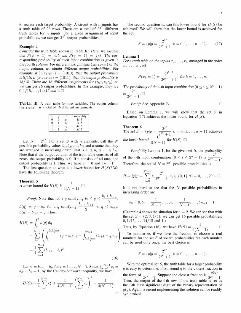
Example 4Consider the truth table shown in Table III. Here, we assumethat P (x = 1) = 4/5 and P (y = 1) = 2/3. The cor-responding probability of each input combination is given inthe fourth column. For different assignments (z0z1z2z3) of theoutput column, we obtain different output probabilities. Forexample, if (z0z1z2z3) = (1010), then the output probabilityis 5/15; if (z0z1z2z3) = (1011), then the output probability is13/15. There are 16 different assignments for (z0z1z2z3), sowe can get 16 output probabilities. In this example, they are0, 1/15, . . . , 14/15 and 1. �

TABLE III: A truth table for two variables. The output column(z0z1z2z3) has a total of 16 different assignments.

x y z Probability0 0 z0 1/150 1 z1 2/151 0 z2 4/151 1 z3 8/15

Let N = 22n

. For a set S with n elements, call the Npossible probability values b1, b2, . . . , bN and assume that theyare arranged in increasing order. That is b1 ≤ b2 ≤ · · · ≤ bN .Note that if the output column of the truth table consists of allzeros, the output probability is 0. If it consists of all ones, theoutput probability is 1. Thus, we have b1 = 0 and bN = 1.

The first question is: what is a lower bound for H(S)? Wehave the following theorem.

Theorem 5A lower bound for H(S) is

14(N − 1)

. �

Proof: Note that for a q satisfying bi ≤ q ≤ bi + bi+1

2,

h(q) = q − bi; for a q satisfyingbi + bi+1

2< q ≤ bi+1,

h(q) = bi+1 − q. Thus,

H(S) =∫ 1

0

h(q) dq

=N−1∑i=1

∫ bi+bi+12

bi

(q − bi) dq +∫ bi+1

bi+bi+12

(bi+1 − q) dq

=

14

N−1∑i=1

(bi+1 − bi)2.

(16)

Let ci = bi+1− bi, for i = 1, . . . , N −1. Since∑N−1

i=1 ci =bN − b1 = 1, by the Cauchy-Schwarz inequality, we have

H(S) =14

N−1∑i=1

c2i ≥

14(N − 1)

(N−1∑i=1

ci

)2

=1

4(N − 1).

The second question is: can this lower bound for H(S) beachieved? We will show that the lower bound is achieved forthe set

S = {p|p =22k

22k + 1, k = 0, 1, . . . , n− 1}. (17)

Lemma 1For a truth table on the inputs x1, . . . , xn arranged in the orderxn, . . . , x1, let

P (xk = 1) =22k−1

22k−1 + 1, for k = 1, . . . , n.

The probability of the i-th input combination (0 ≤ i ≤ 2n − 1)

is2i

22n − 1. �

Proof: See Appendix B.

Based on Lemma 1, we will show that the set S inEquation (17) achieves the lower bound for H(S).

Theorem 6The set S = {p|p =

22k

22k + 1, k = 0, 1, . . . , n − 1} achieves

the lower bound1

4(N − 1)for H(S). �

Proof: By Lemma 1, for the given set S, the probability

of the i-th input combination (0 ≤ i ≤ 2n − 1) is2i

22n − 1.

Therefore, the set of N = 22n

possible probabilities is

R = {p|p =2n−1∑i=0

zi2i

22n − 1, zi ∈ {0, 1},∀i = 0, . . . , 2n−1}.

It is not hard to see that the N possible probabilities inincreasing order are

b0 = 0, b1 =1

N − 1, . . . , bi =

i

N − 1, . . . , bN−1 = 1.

(Example 4 shows the situation for n = 2. We can see that withthe set S = {2/3, 4/5}, we can get 16 possible probabilities:0, 1/15, . . . , 14/15 and 1.)

Thus, by Equation (16), we have H(S) =1

4(N − 1).

To summarize, if we have the freedom to choose n realnumbers for the set S of source probabilities but each numbercan be used only once, the best choice is

S = {p|p =22k

22k + 1, k = 0, 1, . . . , n− 1}.

With the optimal set S, the truth table for a target probabilityq is easy to determine. First, round q to the closest fraction in

the form ofi

22n − 1. Suppose the closest fraction is

g(q)22n − 1

.Then, the output of the i-th row of the truth table is set asthe i-th least significant digit of the binary representation ofg(q). Again, a circuit implementing this solution can be readilysynthesized.

13

VI. CONCLUSIONS AND FUTURE WORK

In this work, we considered the problem of transforminga set of input probabilities into a target probability withcombinational logic. The assumption that we make is that theinput probabilities are exact and independent. For example,in synthesizing decimal output probabilities, we use multipleindependent copies of the exact input probabilities 0.4 and0.5. Of course, if we use physical sources to generate theinput probabilities, there likely will be fluctuations. Also, theprobabilistic inputs will likely be correlated. A future directionof research is how to design circuits that behave robustly inspite of these realities.

In addition to the three scenarios that we presented, thereexists a fourth one that we have not considered: one in whichthe source probabilities are specified and can be duplicated.In this scenario, we would not expect to generate the targetprobability exactly. Thus, the problem is how to synthesizean area or delay optimal circuit whose output probability is aclose approximation to the target value. We will address thisproblem in future work.

VII. ACKNOWLEDGMENTS

The authors thank Kia Bazargan and David Lilja for theircontributions. They were co-authors on a preliminary versionof this paper [16].

REFERENCES

[1] W. Qian and M. D. Riedel, “The synthesis of robust polynomialarithmetic with stochastic logic,” in Design Automation Conference,2008, pp. 648–653.

[2] W. Qian, X. Li, M. D. Riedel, K. Bazargan, and D. J. Lilja, “Anarchitecture for fault-tolerant computation with stochastic logic,” IEEETransactions on Computers (to appear), 2010.

[3] S. Cheemalavagu, P. Korkmaz, K. Palem, B. Akgul, and L. Chakrapani,“A probabilistic CMOS switch and its realization by exploiting noise,”in IFIP International Conference on VLSI, 2005, pp. 535–541.

[4] L. Chakrapani, P. Korkmaz, B. Akgul, and K. Palem, “Probabilisticsystem-on-a-chip architecture,” ACM Transactions on Design Automa-tion of Electronic Systems, vol. 12, no. 3, pp. 1–28, 2007.

[5] K. P. Parker and E. J. McCluskey, “Probabilistic treatment of generalcombinational networks,” IEEE Transactions on Computers, vol. 24,no. 6, pp. 668–670, 1975.

[6] J. Savir, G. Ditlow, and P. H. Bardell, “Random pattern testability,” IEEETransactions on Computers, vol. 33, pp. 79–90, 1984.

[7] J.-J. Liou, K.-T. Cheng, S. Kundu, and A. Krstic, “Fast statistical timinganalysis by probabilistic event propagation,” in Design AutomationConference, 2001, pp. 661–666.

[8] R. Marculescu, D. Marculescu, and M. Pedram, “Logic level powerestimation considering spatiotemporal correlations,” in InternationalConference on Computer-Aided Design, 1994, pp. 294–299.

[9] A. Gill, “Synthesis of probability transformers,” Journal of the FranklinInstitute, vol. 274, no. 1, pp. 1–19, 1962.

[10] ——, “On a weight distribution problem, with application to the designof stochastic generators,” Journal of the ACM, vol. 10, no. 1, pp. 110–121, 1963.

[11] P. Jeavons, D. A. Cohen, and J. Shawe-Taylor, “Generating binarysequences for stochastic computing,” IEEE Transactions on InformationTheory, vol. 40, no. 3, pp. 716–720, 1994.

[12] D. Wilhelm and J. Bruck, “Stochastic switching circuit synthesis,” inInternational Symposium on Information Theory, 2008, pp. 1388–1392.

[13] C. E. Shannon, “The synthesis of two terminal switching circuits,” BellSystem Technical Journal, vol. 28, pp. 59–98, 1949.

[14] H. Zhou and J. Bruck, “On the expressibility of stochastic switchingcircuits,” in International Symposium on Information Theory, 2009, pp.2061–2065.

[15] A. Mishchenko et al., “ABC: A system for sequen-tial synthesis and verification,” 2007. [Online]. Available:http://www.eecs.berkeley.edu/ alanmi/abc/

[16] W. Qian, M. D. Riedel, K. Barzagan, and D. Lilja, “The synthesis ofcombinational logic to generate probabilities,” in International Confer-ence on Computer-Aided Design, 2009, pp. 367–374.

APPENDIX ATheorem 4In Scenario Two, given a set S = {p1, p2, . . . , pn} and atarget probability q, let p be the output probability of the circuitconstructed by the greedy algorithm. We have

|p− q| ≤ 12

n∏k=1

max{pk, 1− pk}. �

Proof: Let w be the output probability of the circuit Cn+1.Since we choose the circuit that has the smallest differencebetween its output probability and the output probability qamong the circuits C1, . . . , Cn+1 as the final construction, wehave |p− q| ≤ |w − q|. We only need to prove that

|w − q| ≤ 12

n∏k=1

max{pk, 1− pk}.

Based on our algorithm, the circuit Cn+1 is a concatenationof n logic gates, each being either an AND gate or an ORgate. Denote the output probability of the i-th gate from thebeginning as wi.

Suppose that P (xn+1 = 1) = pin+1 ∈ {0, 1}. Based on ourchoice of pin+1 , we have

|pin+1 − p∗in+1| = min{|p∗in+1

|, |1− p∗in+1|}.

Thus,

|pin+1 − p∗in+1| ≤ 1

2(|p∗in+1

|+ |1− p∗in+1|).

Our greedy algorithm essures that 0 ≤ p∗in+1≤ 1. Thus, we

further have|pin+1 − p∗in+1

| ≤ 12. (18)

Next, we will show by induction that for all 1 ≤ k ≤ n, wehave

|wk − p∗in+1−k| ≤ 1

2

k∏j=1

max{pin+1−j, 1− pin+1−j

}. (19)

Base case: If the first gate is an OR gate, then we have

w1 = pin + (1− pin)pin+1 .

From Equation (12), we have

p∗in= pin + (1− pin)p∗in+1

.

Thus,|w1 − p∗in

| = (1− pin)|pin+1 − p∗in+1

|.

Applying Equation (18), we have

|w1 − p∗in| ≤ 1

2(1− pin

) ≤ 12

max{pin, 1− pin

}

=12

1∏j=1

max{pin+1−j, 1− pin+1−j

}.(20)

Similarly, if the first gate is an AND gate, we can also getEquation (20). Thus, the statement holds for the base case.

Inductive step: Assume that the statement holds for some1 ≤ k ≤ n− 1. Now consider k + 1. Based on our algorithm,there are four cases:

14

1) The (k + 1)-th gate from the beginning is an OR gatewith one input connected to the output of the k-th gate.

2) The (k + 1)-th gate from the beginning is an OR gatewith one input connected to the inverted output of thek-th gate.

3) The (k + 1)-th gate from the beginning is an AND gatewith one input connected to the output of the k-th gate.

4) The (k + 1)-th gate from the beginning is an AND gatewith one input connected to the inverted output of thek-th gate.

In the first case, we have

wk+1 = pin−k+ (1− pin−k

)wk.

In this case, the relation between the ideal values p∗in+1−kand

p∗in−kis

p∗in−k= pin−k

+ (1− pin−k)p∗in+1−k

.

Thus,

|wk+1 − p∗in−k| = (1− pin−k

)|wk − p∗in+1−k|

≤ max{pin−k, 1− pin−k

}|wk − p∗in+1−k|. (21)

Based on the induction hypothesis, we have

|wk − p∗in+1−k| ≤ 1

2

k∏j=1

max{pin+1−j, 1− pin+1−j

}. (22)

Combining Equations (21) and (22), we have

|wk+1 − p∗in−k| ≤ 1

2

k+1∏j=1

max{pin+1−j, 1− pin+1−j

}. (23)

In the other three cases, we can similarly derive Equation (23).Thus, the statement holds for k + 1. This completes theinduction proof.

Note that {pi1 , . . . , pin} = {p1, . . . , pn}. Thus, when k =

n, Equation (19) can be written as

|wn − p∗i1 | ≤12

n∏j=1

max{pj , 1− pj}.

Based on our algorithm, the final output is either the directoutput of the n-th gate or the inverted output of the n-th gate.In either case, we have

|w − q| = |wn − p∗i1 | ≤12

n∏j=1

max{pj , 1− pj}.

APPENDIX B

Lemma 1For a truth table on the inputs x1, . . . , xn arranged in the orderxn, . . . , x1, let

P (xk = 1) =22k−1

22k−1 + 1, for k = 1, . . . , n.

The probability of the i-th input combination (0 ≤ i ≤ 2n − 1)

is2i

22n − 1. �

Proof: We prove the lemma by induction on n.

Base case: When n = 1, by assumption, P (x1 = 1) =23

.The 0-th input combination is x1 = 0 and has probability

13

=20

22n − 1.

The first input combination is x1 = 1 and has probability

23

=21

22n − 1.

Inductive step: Assume that the statement holds for (n− 1).Denote the probability of the i-th input combination in thetruth table of n variables as pi,n. By the induction hypothesis,for 0 ≤ i ≤ 2n−1 − 1,

pi,n−1 =2i

22n−1 − 1.

Consider the truth table of n variables. Note that the inputprobabilities for x1, . . . , xn−1 are the same as those in the

case of (n− 1) and P (xn = 1) =22n−1

22n−1 + 1.

When 0 ≤ i ≤ 2n−1− 1, the i-th row of the truth table hasxn = 0; the assignment to the rest of the variables is the sameas the i-th row of the truth table of (n− 1) variables. Thus,

pi,n = P (xn = 0) · pi,n−1 =1

22n−1 + 1· 2i

22n−1 − 1

=2i

22n − 1.

(24)

When 2n−1 ≤ i ≤ 2n − 1, the i-th row of the truth tablehas xn = 1; the assignment to the rest of the variables is thesame as the (i− 2n−1)-th row of the truth table of (n− 1)variables. Thus,

pi,n = P (xn = 1) · pi−2n−1,n−1 =22n−1

22n−1 + 1· 2i−2n−1

22n−1 − 1

=2i

22n − 1.

(25)

Combining Equation (24) and (25), the statement holds for n.Thus, the statement in the lemma holds for all n.