transform-based backprojection for volume reconstruction of large format electron microscope tilt...

Journal of

www.elsevier.com/locate/yjsbi

Journal of Structural Biology 154 (2006) 144–167

StructuralBiology

Transform-based backprojection for volume reconstructionof large format electron microscope tilt series

Albert Lawrence, James C. Bouwer, Guy Perkins, Mark H. Ellisman *

National Center for Microscopy and Imaging Research, Center for Research in Biological Structure,

University of California at San Diego, La Jolla, CA 92093-0608, USA

Received 4 August 2005; received in revised form 23 December 2005; accepted 28 December 2005Available online 17 February 2006

Abstract

Alignment of the individual images of a tilt series is a critical step in obtaining high-quality electron microscope reconstructions. Wereport on general methods for producing good alignments, and utilizing the alignment data in subsequent reconstruction steps. Ouralignment techniques utilize bundle adjustment. Bundle adjustment is the simultaneous calculation of the position of distinguished mark-ers in the object space and the transforms of these markers to their positions in the observed images, along the bundle of particle tra-jectories along which the object is projected to each EM image. Bundle adjustment techniques are general enough to encompass thecomputation of linear, projective or nonlinear transforms for backprojection, and can compensate for curvilinear trajectories throughthe object, sample warping, and optical aberration. We will also report on new reconstruction codes and describe our results using thesecodes.� 2006 Elsevier Inc. All rights reserved.

Keywords: Electron microscopy; Tomography; Reconstruction; Bundle adjustment; Nonlinear projection; Radon transform

1. Motivation for this study

In recent years, the format of digital image detectors forthe electron microscope has been progressively increasing.These resulting high-resolution large format images areplaying an important role in determining the three-dimen-sional (3D) structure and function of cells and sub-cellularorganelles at the scale of proteins and protein complexes(Martone et al., 2002a,b). Many of these cellular structurescan extend for tens to hundreds of microns. Large formatdigital detectors are therefore becoming increasingly usefulfor high-resolution data acquisition across multiple lengthscales. Techniques such as serial sectioning tomographyand most probable loss tomography have been developedto deal with the problems of imaging thick sections whichinclude the volume occupied by these large structures (Bou-wer et al., 2004; Soto et al., 1994).

1047-8477/$ - see front matter � 2006 Elsevier Inc. All rights reserved.

doi:10.1016/j.jsb.2005.12.012

* Corresponding author. Fax: +1 858 534 7497.E-mail address: [email protected] (M.H. Ellisman).

The first experimental digital imaging system using char-ge-coupled devices (CCDs) was reported in 1982 with a100 · 100 pixel CCD array directly exposed to 100 keVelectrons. Since then, digital imaging for the TEM has pro-gressed significantly (Roberts et al., 1982). Many digitalimaging systems have been produced between 1982 andthe present (Aikens et al., 1989; Chapman et al., 1989;Daberkow et al., 1996; Downing and Hendrickson, 1999;Fan and Ellisman, 1993, 2000; Fan et al., 2000; Herrmannand Sikeler, 1995; Krivanek et al., 1991; Kujawa andKrahl, 1992; Spence and Zuo, 1998). Digital imaging sys-tems based on CCD technologies, with pixel array sizesup to 4k · 4k, are available for TEM applications at pres-ent. With future camera development efforts promisingmore extensive detectors with formats on the order of8k · 8k and larger, the full image field of the electronmicroscope optics is being utilized. These large area imagesamplify the effects of the inherent distortions and limita-tions of electron optical systems especially in their effectson the quality of the final 3D tomographic reconstructions.

mailto:[email protected]

A. Lawrence et al. / Journal of Structural Biology 154 (2006) 144–167 145

These effects are, of course, well known and methods formitigating them have been previously presented in the liter-ature (Arii and Hama, 1987; Fan et al., 1995; Mastronarde,1997; Penczek et al., 1995). We describe here a set of newtomography techniques, which are designed to addressboth the issues of reconstruction quality and computation-al issues for large image tomograms.

Problems affecting the reconstruction of biological spec-imens are most easily identified through examination of thereconstructed gold fiducial markers in the final volumes.These gold markers are generally spherical and present alarge electron scattering density when compared to the sur-rounding materials. Thus, they are useful for aligning thevarious tilt projections before the backprojection is com-puted. Furthermore, the known geometry of the gold par-ticles and the extensive information concerning theirexpected appearance in the reconstructed volumes providea good indication of the quality of the reconstruction. Theartifacts around the gold particles in reconstructionsrepresent the point-spread function of the reconstructionprocess convolved with the true shape of the particle.

Contrary to the expected appearance, many of the goldparticles in tomographic reconstructions exhibit shapesquite unlike the usual artifacts expected as a result of back-projection reconstruction algorithms (Natterer and Wub-beling, 2001). A single gold particle reconstructed in avolume sliced in the plane perpendicular to the tilt axis isshown in Fig. 1. Fig. 1A is the gold particle reconstructedusing linear backprojection and Fig. 1B is the same particlereconstructed using a backprojection modeled on curvilin-ear electron trajectories. The pre-alignment steps for bothsets of data were identical. Use of the curvilinear modelappears to improve the regularity of the artifact and reduc-es its effect on the other regions of the reconstruction. Thisindicates that methods which compensate for the geometricnonlinearities in the formation of electron microscopeimages will give better reconstructions.

A second problem, also arising from alignment, relatesto the apparent paths of the particles used as markers asthe object is rotated in the electron beam. Applying filteredbackprojection as a reconstruction technique implies thatparticle positions along a given track should be all back-projected through the same point in the object. Also, theimage filter, which is applied before the backprojection,

Fig. 1. A comparison between two typical reconstructed gold particles. (Abackprojection methods of the IMOD backprojection software. (B) The samTxBR. The deviation from spherical bodies is clearly evident in (A) while (B) mhourglass representation of a spherical particle as expected.

should be applied along the particle trajectories. For a sin-gle image filter to work properly, the particle trajectoriesshould all be parallel, independent of the z-coordinate ofthe particle; otherwise the image filter should depend onthe z-coordinate being reconstructed. Our observations ofmarker trajectories in large images indicate that markertrajectories cannot always be made parallel, and that thealignment and filtering problems are inherently three-dimensional.

The misalignment of gold particles arises from a numberof sources. Most notable are the inherent distortions andaberrations associated with electron optics (Arii andHama, 1987). It also can result from errors introducedwhile acquiring data such as positioning errors, pooreucentricity, optical alignment errors, sample warping,and beam-induced mass loss (Fan et al., 1995). It shouldbe noted that optical aberrations and some other nonlin-earities can be eliminated by image transformations. Sam-ple warping and aberrations due to curvilinear electronpaths through the object, on the other hand, are inherentlythree-dimensional, and cannot be eliminated by two-dimensional image transforms.

In addition, the effects of sample warping and curvilin-ear trajectories are confounded in the images and cannotbe easily separated.

Given the intrinsically three-dimensional nature of someof the distortions apparent in large-field electron micro-scope images, we describe a mathematically correct proce-dure for reconstruction, that naturally assumes imagingparticles follow curvilinear trajectories. This is known asthe problem of inverting the generalized Radon transform.If the reconstruction problem can be solved by filtrationfollowed by backprojection, then it is said to be factoriz-able (Defrise, 1995). That the inversion of the generalizedRadon transform is not factorizable has been known forsome time in the mathematical literature (Guillemin,1985), and is highlighted in papers related to seismic imag-ing (Beylkin, 1984; deHoop, 2003). The clearest expositionof the general problem (for small perturbations from thelinear case) is in the paper of Popov (2001) who has shownthat the ‘difference’ between linear filtered backprojectionand the inverse of the generalized transform is a spatiallyvarying Fourier operator which depends on object ratherthan image coordinates. The general theory still leaves

) A typical 10 nm diameter gold particle reconstructed using the lineare particle reconstructed using the curvilinear backprojection methods of

uch more clearly represents a spherical particle. Note that (B) shows the

Fig. 2. An illustration of image formation in a magnetic lens. Electronsscattered at a point in the object travel along helical orbits in a rotatingreference frame and recombine to form the image in the image plane.

146 A. Lawrence et al. / Journal of Structural Biology 154 (2006) 144–167

the general question regarding the degree of improvementpossible from leaving the filter in place and correcting thebackprojection. There are at least two possibilities. One,explored by Mastronarde and his collaborators, is to cor-rect the global backprojection by defining linear backpro-jections on local patches. The local solutions can then beinterpolated together to produce a global reconstruction.This method produces high-quality reconstructions andhas been implemented in the IMOD tomography package(Mastronarde, 1997). An alternative method, which ismore geometrical, is to develop a global nonlinear modelof the electron trajectories, and backproject along thesetrajectories. This is the approach explored in this paper.It may be argued that each approach has its advantagesand disadvantages in terms of theoretical accuracy, butour choice of method is dictated more by computationalissues.

An important issue is the practical aspect of computertime necessary to produce reconstructions. AlthoughIMOD produces high-quality reconstructions, the code isserial, and computation times on large images increase con-siderably. As such, parallel computation was explored asan attractive strategy to reduce turn-around times. To thisend, we first embarked on developing a parallel version ofthe IMOD reconstruction code. The author of the code wasagreeable to this undertaking, but upon further investiga-tion, we found that the local alignment approach addedsufficient complexity to the code as to make a paralleliza-tion effort prohibitively complex. As an alternative, weinvestigated other algorithmic approaches which wouldnot entail local alignment and reconstruction. The mostnatural approach, when using projections which are geo-metrically nonlinear, is to regard each projection map asa set of nonlinear transforms on z-sections which sum toproduce the image. This provides a simple way to introduceparallelization by reconstructing each z-section separatelyvia geometrically nonlinear backprojections. Thus, it canbe said that the original motivation for the developmentof TxBR was to produce a simple and robust parallel back-projection code, which would perform as well as IMOD.

2. Background

2.1. Image formation in an electron microscope

To understand how the distortions affecting tilt-seriesimages arise, we must first consider image formation in auniform magnetic field B. An electron moving in a magnet-ic field can generally be understood to experience a forceaccording to

~F ¼ q~v�~B; ð2:1:1Þwhich acts perpendicular to the plane defined by the veloc-ity vector and the magnetic field lines, where q is the chargeand v is the instantaneous velocity. Electrons moving in amagnetic field will generally orbit the magnetic field lines,moving in helical trajectories. Two electrons scattered into

different angles by the object will each experience a forcecausing the electrons to orbit the field lines. In the equiva-lent of a light optics system, the image is formed when theelectrons once again meet to form the image. Although auniform magnetic field is not a true lens since electronstraveling parallel to the field lines are unaffected by themagnetic fields, the example is instructive.

In real magnetic lenses, to create short focal lengths, themagnetic fields are concentrated using pole pieces (Ruska,1986). This creates rotationally symmetric, but nonuniformmagnetic field lines. In this case, the magnetic field strengthalong the optical axis can be approximated by a function ofthe form of a bell-shaped field

BzðzÞ ¼B0

1þ ðz=aÞ2; ð2:1:2Þ

where B0 is the maximum field in the lens, z is the directionof the optical axis, and 2a is the half-width at half maxi-mum of the field distribution (Reimer, 1993). This approx-imation is useful because it provides analytical solutions tothe electron trajectories. With separation of variables incylindrical coordinates, it can be shown that an image isformed by electrons traveling in helical orbits, in a planethat rotates about the optical axis at a rate given by

xL ¼e

2me

BzðzÞ; ð2:1:3Þ

where xL is the Larmor frequency, me is the mass of theelectron, and e is the charge on an electron. The effect isthat the image is rotated through some angle given byhL = xL Æ time. Fig. 2 shows a cartoon of electron trajecto-ries in the formation of an image in a magnetic lens. It isimportant to note that the degree of image rotation de-pends on the magnetic field strength. Any field inhomoge-neities where

BðzÞ ! Bðr; h; zÞ ð2:1:4Þwill cause varying degrees of rotation through the imageresulting in image twisting such as the commonly observedprojector spiral-distortions (Tsuna and Harada, 1981).


2.2. Spherical aberration

Spherical aberration is significant in electron optics.Spherical aberration results from a lens not having thesame focal length at points near the edge of the lens fieldsvs. the center of the lens field. Spherical aberration general-ly results in a smearing out of a small object into a disk ofleast confusion, D, given by

D ¼ 12Csa

3; ð2:2:1Þ

where Cs is the spherical aberration coefficient and a is thescattering angle (Agar, 1974). Barring other factors thisdisk of least confusion determines the ultimate resolutionof the lens optics. The value of Cs is generally quoted bymicroscope manufacturers and is indicative of the objectivelens performance. When operating at lower magnifications,the large bore projector and intermediate lenses will indi-rectly, through spherical aberration, produce radiallydependent magnifications, that result because of the alter-ation of the focal distance at the edges of the lens fieldresulting in radial-dependent magnification aberrations inthe form of barrel and pincushion type distortions. Fig. 3illustrates the origin of radially dependent magnificationerrors resulting from projector lens spherical aberration.These distortions are usually seen to be small, on the orderof a pixel or two for a 1k · 1k detector. However, withlarger field imaging devices these distortions become moreapparent as a result of their third-order dependence on theradial distance from the center of the lens. Moreover, when

Fig. 3. Spherical aberration indirectly results in radially dependentmagnification in the projector and intermediate lens image formation(A) shows pincushion distortion, while (B) shows barrel distortion. Theblue lines represent aberration free image formation, while the black linesrepresent images formed with a system containing spherical aberration.

combined with other aberrations, radially dependentmagnification errors compound the problem of alignment(Reimer, 1993).

2.3. Tilt geometry

Data acquisition for single axis tilt tomography is per-formed by acquiring images every 1� or 2� while a sampleis tilted about a single axis through a range of typically±60� to ±70�. The process of performing single axistomography itself introduces both differential magnifica-tion as well as differential rotation in the projected images,thereby violating both assumptions of standard linearbackprojection methods. Typically, the degree of violationis minimal for small format images. However, for sampleswith large extended processes imaged in the lower magnifi-cation range using large format detectors, scaling errorsand differential rotation can be significant.

To illustrate the origin of this effect, Fig. 4 shows an exam-ple of a solenoidal magnetic lens and the sample tilt geome-try. The lens effects have been exaggerated to illustrate theeffects of the tilt geometry. The magnetic field strength, Bz,is a function of the height z, the radial distance from the opti-cal axis r, and due to machining tolerances in the pole piece, afunction of q as well. As a result, different subsections of thetilted object will be immersed in varying strengths of themagnetic field resulting in inhomogeneous magnificationand image rotation. These we term differential magnificationand differential rotation, respectively, which are due mostlyto changes in height Dz as the sample is tilted.

Fig. 4. Schematic representation showing the effects of nonuniformmagnetic field lines B and sample tilt geometry for the collection oftomographic tilt series data in a field immersion solenoidal type magneticlens. The magnetic field lines are curved and travel through the center ofthe lens. The field strength is proportional to the line spacing. Close linespacing represents stronger magnetic fields.


To further complicate the object to image transfer func-tion, the object distance will vary from one side of the sam-ple to the other as the sample is tilted. Since themagnification, M, in a lens is given by

M ¼ � d image

dobject

; ð2:3:1Þ

where dimage and dobject are the image and object distances,respectively. With a large magnification objective lens, theobject distance is approximately equal to the focal length ofthe lens, f; therefore, we can write the differential magnifi-cation resulting from the change in object height as

DMM� �Ddobject

dobject

¼ �Dzf; ð2:3:2Þ

where Dz is the change in height as the sample is tilted fromone side of the object to the other. An example calculationwith an objective focal length, f = 3.9 mm, we have

DMM� ð�2:56� 10�4=lmÞ � Dz. ð2:3:3Þ

For a specimen field of view extending 5 lm from thetop to the bottom of the specimen when tilted, this wouldcorrespond to a 0.13% magnification difference. In termsof a 4k · 4k detector, this represents a 5-pixel magnifica-tion distortion as a result of differential magnification dis-tortion due exclusively to sample height and does nottake into account the effect of field strength errors. Theseerrors are well documented and discussed in detail by otherauthors (Arii and Hama, 1987; Fan et al., 1995; Reimer,1993). We therefore defer to previously published datafor further investigation.

2.4. Projective and pseudo-projective distortions

Assuming for the moment that the object is thin, theeffects of departures from the ideal situation of electronsmoving along paths parallel to the axis can be describedin terms of beam divergence and differential rotations.See Fig. 4 for an illustration of nonuniform magnetic fieldsleading to the beam convergence or divergence. Beamdivergence would produce the effects observed in projectivegeometry, a subject first explored systematically by theRenaissance painters (Faugeras and Luong, 2001; Sempleand Kneebone, 1998). These effects would be seen moststrongly in a tilt series as differential foreshortening ofthe lines parallel to the axis of rotation. In effect, as a rect-angular object is tilted around an axis parallel to two of thesides, one of these sides would lengthen and the otherwould shorten as the tilt angle increased. This is the classi-cal trapezoidal distortion of a rectangle seen in perspective.Differential rotations of the beam in a plane normal to thebeam would produce a second kind of trapezoidal distor-

HbRh ¼cos h cos x ð� sin / cos h cos x� cos / sin xÞ ð� c

cos h sin x ð� sin / sin h sin x� cos / cos xÞ ð� c

�

tion, which we might term pseudo-projective. Fig. 2 illus-trates the origin of rotational effects. In this case, lines inthe object parallel to the tilt axis are rotated differently asrotation carries them in a direction parallel to the tilt axis.

The distortion of line segments orthogonal to the tiltaxis is more complex. As a simple case, we characterizethe projection of a line segment through the tilt axis. Atzero tilt the coordinates of this line are given by

ðx; y; zÞ ¼ ðx; c; 0Þ; ð2:4:1Þwhere c is a constant. Rotation Rh by an angle h around thetilt axis is given by

Rhðx; c; 0Þ ¼ ðx cosðhÞ; c; x sinðhÞÞ. ð2:4:2Þ

Assuming that the electron beam rotates at a constant ratein the z-direction, and that the rate constant (helicity) is b,we obtain a formula for the projection Ha onto the image

HbRhðx; c; 0Þ ¼ ðx cosðhÞ cosðxÞ � c sinðxÞ;c cosðxÞ þ x cosðhÞ sinðxÞÞ; ð2:4:3Þ

where

x ¼ bx sinðhÞ.Treating the cosine as a scaling factor x 0 = x cos (h), weobtain

HbRhðx; c; 0Þ ¼ ðx0 cosðbx0 tanðhÞÞ � c sinðbx0 tanðhÞÞ;x0 sinðbx0 tanðhÞÞ þ c cosðbx0 tanðhÞÞÞ.

ð2:4:4Þ

Since the helical rotation preserves the radius of the trans-formed point in the x–y plane, we can simplify the expres-sion on the right-hand side by using polar coordinates (r,u)

r ¼ffiffiffiffiffiffiffiffiffiffiffiffiffiffiffic2 þ x02

p; u ¼ arctan

x0

c

� �þ bx0 tanðhÞ. ð2:4:5Þ

Making the substitution

x0 ¼ffiffiffiffiffiffiffiffiffiffiffiffiffiffir2 � c2p

; ð2:4:6Þwe obtain the equation of a spiral curve

u ¼ arctan

ffiffiffiffiffiffiffiffiffiffiffiffiffiffir2 � c2p

c

!þ b tanðhÞ

ffiffiffiffiffiffiffiffiffiffiffiffiffiffir2 � c2p

. ð2:4:7Þ

In effect, straight-line segments orthogonal to the tiltaxis are mapped to segments of spiral curves. Because ais small, this effect is not readily apparent, but large imagesof grids may exhibit slight bowing of the horizontal gridlines. Lines parallel to the z = 0 plane would exhibit similardistortions as they are rotated around a vertical tilt axis.

Without writing out the details, a similar derivationgives the projection of a point (x,y,z) tilted by an angle hat a pitch angle / around a tilt aligned along the y-axis.We can write this projection in matrix notation

os / sin h cos xþ sin / sin xÞos / sin h sin x� sin / cos xÞ

�; ð2:4:8Þ


where

x ¼ bðx sin hþ y sin / cos hþ z cos / cos hÞ. ð2:4:9Þ

From this equation, we can see that a helicity factor b onthe order of 10�6 can produce significant alignment dis-placements on the edge of the image. Beam divergencehas effects of a similar magnitude.

Projective effects of both types can be quantified asscaling coefficients in a generalized projective transform.We discuss this below. From our numerical investigationswith actual tilt-series data, the spatial scale of the scalingtransform coefficients can be a factor of 10�6–10�7 small-er than the dimensions of the object, yet the transformproduces observable distortions in large images (Fanet al., 1995).

For thick sections, the curvilinear nature of the rays canalso be a factor. Nonlinear, rather than projective, trans-forms are necessary to provide a model for the observedphenomena. We also will discuss some of the issues, whichmay arise when it is necessary to model both the projectivegeometry and the curvilinear geometry of the pathssimultaneously.

2.5. Mass loss and other problems

Thin objects placed in a high-energy electron beam willgenerally show some mass loss due to displacement ofatoms. This mass loss is somewhat dependent on localmaterial characteristics, so it is not uniform. This, in turnleads to some degree of warping of the sample, and nonlin-ear, nonuniform geometric distortions on the order of afew percent. Although these effects can be reduced consid-erably by pre-exposure of the sample, they are still observa-ble. Because the effects over many observations, as with atilt series, are cumulative and can cause errors in alignmentthese effects will degrade the quality of reconstructions.Furthermore, these effects are unpredictable, and mayinteract with optical effects in complicated ways. As withthe geometric and optical effects we discuss above, theproblems increase in magnitude with increases in samplesize.

2.6. Implications for tomography

Analysis and our observations of reconstructions basedon large images confirm that commonly used reconstruc-tion processes do not give the expected reconstruction ofthe gold particles. This, in turn, has led us to believe thatthe X-ray transform model often built into the tomograph-ic reconstruction process is not accurate enough for ourpurposes. For example, motion along curvilinear trajecto-ries leads to a theory of image formation which departsin several significant ways from the classical model. Asdescribed above, beam helicity and small beam divergencescan produce effects analogous to pinhole camera projectioneffects.

Distortion effects have been observed and reported inthe literature. Mastronarde et al. report on distortions,which are locally linear, but not projective, and proposea method for computing tomograms, which compensatefor such distortions (Mastronarde, 1997). The softwarepackage IMOD is designed around these ideas. Electronmicrographs of rectilinear grids as reported by Fan et al.show recognizable trapezoidal distortions (Fan et al.,1995). Frank and co-workers have observed local opticaldistortion in the crystallography of purple membranes(Frank et al., 1993). Brandt and co-workers have devel-oped methods for solving the alignment problem in thecase where classical projective distortions are present(Brandt et al., 2001a,b).

3. Objectives of the study

Given the problems outlined above, the task of tomo-graphic reconstruction is somewhat akin to the job of accu-rately mapping the organs of a jellyfish swimming at adistance in the ocean and photographed through the bot-tom of a soft drink bottle. This is, of course, somewhatof an exaggeration, but given the requirement for high pre-cision in our reconstructions, the simile is apt. To continuewith the analogy, the various movements of the animal, thebending of the light rays in the seawater, and the opticaldistortions of our camera may produce totally confoundedeffects. On the other hand, we can accomplish our task toany specified accuracy with enough visible particles embed-ded in our subject and with enough views from various per-spectives. The problem is to obtain data of sufficientquantity and quality.

The objectives of the research, from which results arereported here, were to:

1. Develop a computationally efficient model of the opticsof the electron microscope, which can be applied to theproblem of determining the effective projective maps.

2. Develop image alignment procedures, which can beapplied to the case of nonlinear projections.

3. Adapt the backprojection reconstruction method to thegeneral case of curvilinear electron trajectories.

The initial and key step of the tomographic reconstruc-tion process is to mark and track a sufficient number offiducial particles in the object. Once this is accomplished,two coupled problems remain to be solved. The first prob-lem is the determination of the three-dimensional configu-ration of these markers in the object and the second is todescribe the proper nonlinear transformations from theobject to the images. Bundle adjustment methods andreconstruction via geometrically nonlinear transformsprovide a set of very powerful tools for this work.

Projection models for the imaging transforms may berecovered from information in the tilt views, jointly withthe three-dimensional positions of the distinguished mark-ers, given that sufficient distinguished and stable markers


are present. The most common class of methods for accom-plishing this is called bundle adjustment, from the notionthat the projection or imaging transforms are along a bun-dle of rays from the object configuration to the image(Triggs et al., 2000). The calculation adjusts the rays, ormore generally, curved trajectories, along with the three-di-mensional configuration. The main objective of our studywas to apply these tools in the general context of wide fieldelectron tomography.

4. Tomographic reconstruction

After image acquisition, the reconstruction process isdivided into three phases. The first phase is to identifythe precise location of a set of image features consistentacross the image series. The second phase of the recon-struction is to develop geometric correspondences betweenthe configurations of features in the images, and if neces-sary to transform the images geometrically to bring the fea-tures into better alignment. This is the alignment process,and can be done automatically once feature tracking isaccomplished. The third and final part of the process isto construct a three-dimensional model of the object itselffrom the image data and the projection transforms. Thisis the reconstruction proper. We describe this in the sectionon the generalized Radon transform.

4.1. Alignment

The reconstruction process depends upon constructingan accurate model of the projections from the object tothe image. This is the essence of the alignment process.Alignment depends, in turn, upon the accurate identifica-tion and tracking of image features common to all of thetilt views. In essence, the reconstruction quality can onlybe as good as the alignment accuracy permits. Therefore,good reconstructions begin with precise location and track-ing of image features. To compensate for various opticaleffects, large numbers of features must be tracked across60 or more images. Automated or semi-automated meth-ods for tracking considerably reduce the effort needed toget a good alignment.

In practice, the process of tracking image features andthe process of aligning the markers in the images are notalways separate and well-distinguished steps. This isbecause methods that depend strictly on feature identifica-tion and location may fail for even the simplest of featureclasses. The prescription for handling this problem is totrack the features approximately, construct a rough align-ment, and feed the results of the rough alignment intothe tracking, to get a better fix on the location of thefeatures being tracked.

Leaving aside the details of the tracking problem, thekey issue in alignment is the determination of two sets ofunknowns, the three-dimensional positions of the markedfeatures in the object and the projections from theobject to the tilt images. The projection transforms and

the positions of the markers are both unknown a prioribecause the transforms act on the coordinates of the mark-ers. Thus, simultaneous determination is a nonlinear prob-lem, even when the projections are linear.

Because of the essential nonlinearity of the alignmentproblem, ordinary linear techniques, such as regression,will not work. The unknowns, in this case, satisfy a nonlin-ear relation, which must be solved by other means. In ourcase, the geometric transforms that represent the process ofimage formation are also nonlinear. This complicates thesituation, but if methods of sufficient generality are usedto solve the basic problem, then these methods may beextended to the case of geometrically nonlinear mappings.Bundle adjustment techniques extend naturally to the caseof curvilinear trajectories.

In our case, we can pose the bundle adjustment problemas an optimization problem. In particular, we can use alge-braic expressions relating the 3D positions to the actualmarked features in the images. Using these expressions,we may calculate the total re-projection error, that is, thesum squared distance between the marked points, and theprojected points (under the calculated transforms). Giventhat there is an algebraic expression for this quantity, cal-culating a minimum for the re-projection error is a routineapplication of optimization techniques. Obtaining therequired parameters for both the transforms and the 3Dmarker positions is automatic. Generally, we track enoughpoints so that the minimum solution is overdetermined anduse conjugate gradient optimization techniques for thecomputations.

After tracking and aligning the markers, we must pro-duce aligned images. The main purpose of this step wasto produce a series of images in which the markers movehorizontally in successive tilts when viewed along the opti-cal axis. This, in turn aligns the standard one-dimensionalr-weighted filter (or one of its avatars, such as the Shepp–Logan filter) with the motions of the images. In this case,the r-weighted filter is more accurate. This is because geo-metrical alignment in which the fiducial marks move hori-zontally is a fundamental requirement of application ofsuch filters. Alignment can be performed by simple rota-tion, by a projective map (homography) or a nonlinearremap. Requiring that the marks move horizontally (thatis, the y-values are constant) gives some simple polynomialalgebraic expressions for the remap transforms. The remaptransforms can be calculated by a simple regression on thepolynomial coefficients.

4.2. The generalized X-ray transform and its inversion

Once the tracking and alignment problems are solved,the reconstruction problem can be posed in more precisemathematical terms. In essence, we must reconstruct anobject with a three-dimensional density distribution fromintegrals along trajectories, where the image intensity ateach point in each of the images represents a line integralalong a specific trajectory. This problem of inversion of


the generalized ray transform (Popov, 2001) is usually illposed and is solvable only in some general sense (Quinto,1993). Therefore, at best, inversion can be performed onlyup to a well-characterized indeterminacy. We note thatmodel trajectories can be calculated from the transformscalculated in the alignment step but for our methods, theparticle trajectories need not be explicitly calculated.

Because electrons move in curvilinear trajectories underobservational conditions in the electron microscope, we areled to consider the general situation of integrals alongcurved paths, see Fig. 5. In essence, we must reconstructan object with a three-dimensional density distributionfrom image intensities. The image intensity at each pointin the image represents the exponential of a line integralalong a specific trajectory through the object.

Transforms by means of line integrals along curvilineartrajectories have been studied under the designation of gen-eralized X-ray transform. The generalized ray transform isdefined for a family of curves (for example, a family ofhelices)

C ¼ fcðX ;xÞg; ð4:2:1Þwhere X denotes a point in the object and x denotes adirection through the point X. In particular, x can be takenas the direction cosines of the tangent to c at the point X

where the curve passes through a plane in the object. In or-der for the transform to be well-defined, g must satisfysome consistency conditions. These conditions are simplya mathematical formalization of the physical situation gen-erally assumed for an electron microscope. Thus, a set oftilt-series views is a sampling from a curvilinear ray trans-form and the parameter x describes an orientation of theobject.

We can define the generalized ray transform as follows:

vðx;xÞ ¼Z cðX 1;xÞ

cðX 0;xÞu½cðrÞ�dr; ð4:2:2Þ

where the integral is taken along the curve c (X,x), u is thedensity of the object, and v is the integrated density. Thequantity r is the arc length parameter. The pointsc (X0,x) and c (X1,x) represent the entry and exit pointsof the trajectory through the object, respectively. Because

Fig. 5. The standard linear backprojection geometry vs. transform-based badensities in the projection images at each tilt angle / are pulled back in aninformation on the object density through a backprojection operator. This is lin/ are pulled back along curved trajectories to provide the three-dimensional o

of the consistency conditions, it is possible to restrict theset of points on which n is defined to some lower-dimen-sional subset of the three-dimensional region, for examplean imaging plane.

4.3. Reconstruction from generalized projections

As above, we denote the object density by u (X) and theX-ray transform by m (x,x). In many cases of practicalinterest, it is possible to find u (X) from m (x,x). The solu-tion is well known when the paths of the particles arestraight lines; this is the problem of inverting the X-raytransform. More general cases have been studied in geo-physics (seismic rays), and various types of tomography(optical tomography, electrical impedance tomography,acoustic imaging, etc.) (Natterer and Wubbeling, 2001).The theoretical justification for generalized backprojectionmay be found in the mathematical literature. Because theimaging process can be modeled as a generalized X-raytransform, the problem of reconstructing a three-dimen-sional volume from a series of generalized projections isthe problem of inverting a generalized X-ray transform.As we have shown in Section 2.4, generalizing to the non-linear trajectories is necessary because the nonlinear trajec-tories represent significant departures from orthogonalprojective maps.

The literature on the problem of reconstruction fromprojections along curvilinear trajectories is much morefamiliar to seismic scientists than to EM tomographers,but the basic theory applies directly to the electron tomog-raphy problem with known curvilinear trajectories. Beyl-kin’s (1984) paper discusses the case of generalizedRadon transforms in arbitrary dimensions and demon-strates an inversion formula, which is related to the famil-iar composition of an r-weighted filter followed by abackprojection. This formula reduces to inversion of thegeneralized curvilinear ray transform in two dimensions.Denysuk presents another proof of the generalized Radoninversion formula in his 1994 paper, and derives a similarformula for multidimensional ray transforms (Denysuk,1994). Both of these papers rely upon the theory of pseu-do-differential operators, which is the proper context when,

ckprojection. The black bodies represent gold fiducial markers. (A) Theorthogonal direction and summed together to provide three-dimensionalear backprojection. (B) The densities in the projected images at each anglebject density. This is transform-based backprojection.


due to geometric nonlinearities, the familiar Fourier slicetheorem does not apply. Sharfutdinof, in his 1999 lecturenotes, presents an implicit two-dimensional inversion basedon a partial differential equation (Sharafutdinof, 1999).The method was derived by Mukhometov and reportedin the geophysical literature (Mukhometov, 1975a,b).Romanov reduces a multidimensional reconstruction prob-lem to an integral equation (a Volterra equation of the sec-ond kind) under the following assumptions: (1) eachtrajectory resembles a reflection off a point in the regionto be reconstructed, (2) the trajectories all start and endin a hyperplane, (3) the set of trajectories is invariant withrespect to translation in this hyperplane, (4) the trajectoriessatisfy a set of continuity conditions, and (5) each point ofthe region to be reconstructed is assigned to a unique tra-jectory (Romanov, 1974). Ehrenpreis considers the inverseproblem as a generalization of the Fourier slice theorem(Ehrenpreis, 2003; Natterer and Wubbeling, 2001).

For the purposes of subsequent discussion, we willadapt the viewpoint of Beylkin and Denysuk. Under aset of assumptions which includes our model of imagingin the electron microscope, we can derive a formula similarto the following:

uþ Tu ¼ R�Kv; ð4:3:1Þwhere u is the object density, m is the image intensity, T is aconvolution operator (or pseudo-differential operator), R*

is a generalization of the backprojection operator, and K

is a an operator analogous to the usual r-weighted filter(Beylkin, 1984; Denysuk, 1994). If the departure of the cur-vilinear rays from straight lines is small, then Tu is small.Formulas similar to this have been proven when the pathsare geodesics (seismic rays), the symmetries of the problemreduce the dimensionality (sinogram case), or the set ofdirections is complete. The actual expression of (4.3.1) isin terms of pseudo-differential operators, which are gener-alizations of the usual Fourier transforms which appear insome inversion formulas.

Popov (2001) presents an alternative form of the opera-tor equation in two dimensions. In his formulation

u ¼ R�1z v; ð4:3:2Þ

where Rz is the generalized Radon transform arising from anonlinear perturbation of a linear Radon transform. Thegeneralized Radon transform is decomposed as a series ofoperators

R�1z ¼ ðI þ QzÞ

�1ATz R�1; ð4:3:3Þ

where I is the identity operator, Qz is a pseudo-differentialoperator, AT

z is the adjoint of an integral Fourier integraloperator, and R�1 is the inverse of the linear Radon trans-form. From the various formulations of the inverse prob-lem for generalized Radon transforms and X-raytransforms in two and three dimensions, we should expectthat the general problem of the inversion of the generalizedX-ray transform in three dimensions is nonlocal andnonfactorizable. This is because all object coordinates

enter explicitly into the operators in the nonlinear case,and the inversion of the linear three-dimensional X-raytransform is nonlocal. As a consequence, solutions basedon local data introduce errors. A discussion of the magni-tude of these errors is beyond the scope of this paper, but ingeneral the magnitude depends on the departure of the tra-jectories (4.2.2) from straight lines.

In practice, a finite set of N images is taken where thesource is in a different direction relative to the object foreach image. We can label the images by the direction ofthe source [xi: i = 1,2, . . . ,N]. Due to mechanical errors,field fluctuations, and all of the effects discussed above,the set of paths for the particles that produce the imagesare not known precisely. Under the assumption that theparticles travel in straight lines, and the image is a set ofintegrals along an orthogonal projection, this is the usualalignment problem. In the more general case, we can refor-mulate the alignment problem as described below.

Once point to point correspondence for particle paths isestablished, an inversion formula may be applied.Although the expressions for the operators K and T in(4.3.1) can be calculated in principle, explicit formulas havebeen worked out in only a few specific cases. If R is anorthogonal X-ray transform, R* is the backprojection, K

is the well-known r-weighting filter and T is zero. Other-wise, even when explicit expressions for the particle paths(or the shadowgram projection) are known, the operatorK is spatially varying, and therefore requires extensivecomputation to evaluate precisely. The situation for theoperator T is even worse. Generally, we may only estimatethe error due to its neglect. Also, in practice, it is not pos-sible to obtain a set of views in all rotational directions.This is the missing wedge problem as in the case of thestandard X-ray transform (Frank, 1992; Natterer andWubbeling, 2001).

In our present investigations, we have limited ourselvesto the correction of misalignment errors due to the effectsof curvilinear trajectories. Thus, in our reconstructions, Kis taken as the usual r-weighted filter, or one of its close rel-atives, such as the Shepp–Logan filter, and that the term Tu

is neglected. We recognize that this is an approximation,but the purpose of our work was to test the hypothesis ofprojective and nonlinear effects by investigating what weestimate is the largest contributor to the reconstructionerror, i.e., the misrepresentation of the trajectories in thebackprojection. We believe that the error in the filter issmall, because the shape of the actual point-spread func-tion (with curvilinear trajectories) is within a pixel or soof the shape of the standard point-spread functionobtained in the case of orthogonal projections. Computa-tional estimates for the magnitude of Tu may be provided,in principle, by phantoms calculated under variousassumptions concerning the instrument optics, or by anaccurate and explicit approximation to the backprojectionmap. The latter can be accomplished as a specific applica-tion of the inverse function theorem, but this remains aswork to be done.


Although several linear methods may be applied toreconstruction, we have chosen to work with a backprojec-tion algorithm because of its computational simplicity(Natterer and Wubbeling, 2001). Inversion of the corre-sponding problem can be studied in the context of linearalgebra, using the Kaczmarz method or the singular valuedecomposition (and references therein), but these methodsare computationally costly and are not well suited for useon the desktop computers and workstations we used in thisinvestigation (Natterer and Wubbeling, 2001).

5. Mathematical methods

5.1. Development of projection models and application to thealignment problem

To align a series of exposures, one must define a suitablemodel for the optics. The general projective model, whichmodels the optics of straight-line trajectories, and is ageneralization of pinhole camera models, is given by thefollowing formula:

kx

y

� �¼ P ½Gjt�

X

Y

Z

264

375

264

375; ð5:1:1Þ

where P is a projection, G is a nonsingular lineartransform, t is a translation, and k is a scaling func-tion on the (X,Y,Z) coordinates. In this case, the pro-jection map gives the destination in the imaging planeof a trajectory c, which passes through the point(X,Y,Z) in the object. If the trajectories were allstraight lines, as in the case of X-rays, we would havea classical projective map and G would be an orthog-onal matrix (Faugeras and Luong, 2001; Heyden andAstrom, 1997). Bundle adjustment calculates the scalingtransform k, the linear transform G, and the three-di-mensional transform, t, simultaneously with the(X,Y,Z) coordinates of the marker points, which wecall the XYZ model.

Once a projective model is calculated, higher-order opti-cal aberrations and some degree of sample warping may beincluded by the following model:

x

y

� �¼ P ½Gjt�

X

Y

Z

264

375þ ½X Y Z �Q

Z

Y

Z

264

375

264

375; ð5:1:2Þ

where Q is a 3 · 3 symmetric matrix, which represents ahomogeneous quadratic form. This formula derives fromthe first three terms of the Taylor expansion of a warpingmap

W : R3 ! R2 ð5:1:3Þfollowed by a projection. Although one might assume thatthe trajectories c as discussed above should be segmentsof parabolas, elimination of variables shows that thetrajectories are actually given by quartic polynomials.

These polynomials give the backprojection map explicitly,but explicit computation would be time-consuming andinconvenient so we do not use this approach.

The expansion can be carried to cubic terms, if higher-order approximations to paths through the sample are anissue. Each increase in the degree of the map requires thedetermination of additional parameters, and thus asubstantial increase in the number fiducial markers. Fur-thermore, cubic polynomial projection maps cannot besolved for explicit trajectories, by a classical result in alge-bra, so explicit backprojection maps can only be given for alimited set of possible trajectories.

Given both projective and nonlinear contributions, theproblem is to combine them correctly in a general model.Putting scaling functions and nonlinearities into the samemodel and attempting simultaneous determination of allof the parameters can lead to singularities. We first con-sider a purely projective map. In order for the projectivemap to be well-defined on the volume comprising theobject, the scaling function must not be zero there. Thescaling function is an affine map, so the plane deter-mined by the scaling function should not pass throughthe object. In terms of projective geometry, this is theplane at infinity, and with the beam divergences presentin the electron microscope, the plane at infinity doesnot pass through the volume of the reconstruction. Inparticular, a simultaneous calculation of an XYZ modeland projective maps will not produce unwanted singular-ities. When nonlinear terms are included in the model,then an attempt to calculate an XYZ model and projec-tions will lead to unwanted results. In this case, a localminimum for the total error may give a scaling functionwhich goes to zero inside the volume of the object. Thisproduces a singularity. In fact, it is possible to have a setof points within the object which project to the fiducialpoints in the image, via a nonlinear map, but at thesame time the projection map is singular on a surfacewhich passes through the object. This singular surface,by necessity, does not pass through the points of theXYZ model, and its image is a curve which does notpass through the fiducial points but the map itself doesnot represent anything which is likely to occur in an elec-tron microscope. One way to avoid this problem is toseparate the effects of the scaling function and the non-linear terms, by calculating a projective map and theXYZ model in the first stage. This is the initial bundleadjustment. In the second stage, the XYZ model andthe coefficients of scaling functions are kept constant,and a general polynomial map projecting from three totwo dimensions is calculated by regression techniques.The points used in the regression are the XYZ modeland the fiducial points. A description of the details ofthe projective geometry can be found in the work ofSemple and Kneebone (1998).

In effect, we handle the problem of the singular surfaceby keeping it at infinity. More explicitly, we can modifyformula (5.1.2) as follows:


kx

y

� �¼ P ½Gjt�

X

Y

Z

264

375þ ½X Y Z �Q

X

Y

Z

264

375

264

375; ð5:1:4Þ

where the coefficients of k (which is a function of X, Y,and Z) and the points of the XYZ model are determinedby minimizing the reprojection error associated with(5.1.1) and are kept as constants. Thus, (5.1.4) can be usedto define a second minimization problem, but because thecoefficients of the scaling function k and the XYZ modelare held constant this becomes a linear problem and canbe solved by regression techniques. This avoids the prob-lem of singularities associated with the scaling function.One pleasant aspect of this problem is that the array ofcoefficients, Q, must be symmetric. To produce betterapproximations, we can also add a third-order cubic form(with appropriate symmetries) to the right-hand side of(5.1.4). A symmetric formula for the cubic model definesour preferred form for cubic corrections, and the approachwe use in our software.

To calculate how many fiducial points are necessary foreach model, we note that the number of coordinates for thegold particles in the object is 3 T where T is the number oftracks. The number of transform coefficients is 11 for eachprojective transform, 23 for each projective transform plusquadratic coefficients, and 41 coefficients for each projec-tive transform plus quadratic and cubic corrections. If N

is the number of tilts, then the projective model requires11 N coefficients, and so forth. In order for the model tobe well determined or overdetermined, a theorem in alge-braic geometry which generalizes the dimension-countingarguments of linear algebra (Hartshorne, 1977) tells us thatthe total number of 2D fiducial coordinates must be greaterthan the total number of 3D gold particle coordinates inthe object plus the number of transform coordinates. Inthe case of the projective model, this inequality reads 2 N

T > 11 N + 3 T; in the case of the quadratic model 2 N

T > 23 N + 3 T, and so forth. Given a tilt series of 60 tiltswith 20 tracks; the left-hand side of the inequality is 2400,and the right-hand side is 720, so the problem is overdeter-mined. For tilt series of about 60 images, the 20–40–60 rulefor projective, quadratic, and cubic models gives goodnumbers for a statistical averaging of about three inputcoordinates for each output coordinate. In any case, Mat-lab has built-in routines which detect when a problem isunderdetermined, by the condition numbers of the matricescalculated in several of the subroutines. These routines gen-erate error messages when too few fiducial marks are used.

5.2. Bundle adjustment computation

As defined in the literature (Triggs et al., 2000), bundleadjustment is the problem of refining a discrete reconstruc-tion of the markers to produce jointly optimal 3D positionsfor the markers and parameter estimates for the projectionmodel which we assume fits the optics of the instrument.To accomplish this, we minimize some cost function that

quantifies the total re-projection error as defined below.Originally the term bundle adjustment arose from the situ-ation of a series of pinhole camera images. This was theidea that ‘bundles’ of rays leave each 3D feature and con-verge on each camera center, in a series of images which are‘adjusted’ optimally with respect to both feature and cam-era positions. In our case, we replace rays by general curvi-linear trajectories, and the pinhole camera by a generalprojection model, as in formulas above.

The model coordinates are given by a set of vectors:

M ¼ fðX i; Y i; ZiÞji ¼ 1; 2; 3; . . . ; Tg; ð5:2:1Þwhere T is the number of particles tracked through the tiltseries.

The track coordinates are given by a doubly indexed setof vectors: Bundle adjustment computation

T ¼ fðxpij; y

pijÞji ¼ 1; 2; . . . ; T ; j ¼ 1; 2; . . . ; V g; ð5:2:2Þ

where V is the number of views. We use two indices to de-scribe the track number and the tilt number, while thesuperscript p emphasizes that the coordinates are in theprojected images.

Step 0: An initial crude estimate for the (X,Y,Z) coordi-nates of the model points M is computed by a triangulationprocedure using data at low tilt angles. We can assume thatthe images are rotated so that the tilt axis is projected par-allel to the y-axis in the image of unrotated object. In thiscase, we can take X = xp and Y = yp, where (xp,yp) are thecoordinates of the marker point in the nonrotated view.The apparent position of the point moves to((xp � x0) cos (h) � Z sin (h),yp) where x0 is the position ofthe tilt axis, h is the tilt angle, and Z is the (unknown)coordinate.

Step 1: Initial values for l, t, and G (5.1.1) are calculatedby linear regression from the initial estimate of the modelcoordinates.

Step 2n: The initial estimates are refined by a processcalled bundle adjustment. This is an optimization process,where the objective function E is defined by:

E ¼XT

j¼1

XV

i¼1

M1j

X i

Y i

Zi

264

375� kjx

pij

0B@

1CA

2

þXT

j¼1

XV

i¼1

M2j

X i

Y i

Zi

264

375� kjy

pij

0B@

1CA

2

. ð5:2:3Þ

In this formula Mkj is row k of [Gjt] for the jth view. Weemploy a gradient-following procedure to determine valuesfor Mjk, kj, and the model coordinates T. In our case, weuse the method of conjugate gradients for our optimiza-tion. Note that (5.2.3) specifies a projective model for thetransforms; similar expressions can be used for the qua-dratic, or cubic cases. Our approach, however, is to calcu-late the projective model by our optimization procedureand leave the nonlinear terms to a subsequent step.


Step 2n + 1: New values for lj, t and G are calculated bylinear regression from the values given by the optimization.This step is included to speed convergence.

Steps 2n and 2n + 1 are repeated until a predeterminedconvergence criterion is met. This optimization proceduregives us a projective model. A post-processing step usingthe model described by (5.2.3) gives us the nonlinear cor-rections. In this step, the scaling factor and model coordi-nates are held constant. A simple regression can then beused to give the remaining parameters. Computation ofthe backprojection R* requires the polynomial approxima-tion to the projection R along electron paths g. As anexample of the type of equation that must be solved in eachimage at tilt angle h, and for each fiducial marker j, thefollowing quadratic approximation is provided:

P quadratici ðxj; yj; zj; hjÞ

¼ ahi1x2

j þ ahi2xjyj þ ah

i3xjzj þ ahi4y2

j þ ahi5yjzþah

i6z2j

h in

þhbh

i1xj þ bhi2yj þ bh

i3zj þ chi

io 1

dh1xj þ dh

2yj þ dh3zj þ 1

( )ði ¼ 1; 2Þ.

ð5:2:4Þ

Here, the index i = 1,2 is required to map from threedimensions to two dimensions. The index h in the coeffi-cient superscripts reinforces the fact that there is a separateset of coefficients for each tilt angle. The first term in (5.2.4)is the quadratic correction to the electron paths, the secondterm is the affine correction to compensate for translation,rotation, skew, and scaling, and the overall multiplicativeterm contains projective scaling corrections. Since 23parameters (two for each a, b, c, and d in Eq. (5.2.4)) mustbe solved for simultaneously in each projection, a sufficientnumber of fiducial markers are required for a solution.

5.3. Backprojection

Our reconstruction methods are an extension of thestandard orthogonal backprojection process (Nattererand Wubbeling, 2001). The EM projections are filteredby means of a modified r-weighting. The transforms calcu-lated via the bundle adjustment are then applied to pointsin z-sections of the object space to obtain correspondingpoints in the electron microscope images. The density val-ues of the points in the filtered images are pulled back tothe point in the object and averaged into the density valuethere. Formally

uðX ; Y ; ZÞ ¼ 1

N

XN

i¼1

viðT iðX ; Y ; ZÞÞ; ð5:3:1Þ

where u is the reconstructed value at (X,Y,Z), N is thenumber of EM projections mi is the ith aligned filteredEM view, and Ti is the transform for the ith projection cal-culated via the bundle adjustment. When presented in thisform, we have a natural choice for coarse-grained parallelcomputation, in which the reconstruction along each

Z-slice on the left-hand side is calculated on a different pro-cessor. As we will discuss below, this form also permits theuse of clever tricks for the computation of the transform.At this point, we must note that the backprojection canbe calculated by reconstructing pieces of the object by lin-ear transforms and then patching the pieces together by theappropriate ‘‘gluing’’ maps. This is computationally awk-ward, and inevitably introduces additional errors into thereconstruction process, as the gluing maps are themselvessubject to error unless we understand the global geometryof the image formation process. Nevertheless, this couldbe done by the local application of the Fourier slice theo-rem, thus permitting fast reconstruction. If speed is themost important factor, a local approach may be themethod of choice. This is the approach used in the IMODreconstruction package (Kremer et al., 1996).

6. Software

6.1. Development environment

Because of the depth of capabilities of the IMOD soft-ware system our system has been developed, to a largedegree, as an extension of the IMOD packages. Whereverpossible we have used the same file formats as used byIMOD. In particular image data files, fiducial data files,xyz coordinate models, and re-projection error data arethe same as those in IMOD. This allows us to use the3dmod program and its plugin modules to view data andreconstructions, refine fiducial models, and use the beadfixer to improve tracking. The only exception is thealignment transform files, which do not apply to ourmethodology.

We have chosen to develop our software in Matlab(Mathworks, 2002a). Current commercial scientific soft-ware systems such as Matlab have a number of distinctadvantages, not the least of which are the error reportingand accessibility of the current state of all current programvariables. This has greatly reduced the time usually spent inprogram debugging, and has decreased code developmenttimes considerably.

Matlab has a large number of solid and precise numer-ical routines including those for optimization and eigenval-ue determination. The latter routines are derived fromLAPACK, which is a standard linear algebra and matrixanalysis package (Anderson et al., 1999). For our purposes,the conjugate gradient optimization and singular valuedecomposition routines are central to our bundle adjust-ment procedures (Anderson et al., 1999; Mathworks,2002b).

Because of just-in-time compiling Matlab also has somesignificant speed advantages over a purely interpretativesoftware language. As noted above we are presently dealingwith large images, and our completed tomograms canoccupy many gigabytes of disk storage space. Tomographicreconstruction is a large-scale computing problem. Becausethe performance times for Matlab are not unreasonably


large when compared with those of compiled code, we candevelop our software with real data, and with the exceptionof the most time-critical routines, use the code we havedeveloped in a production environment.

With respect to the most computation-intensive portionof our code, the backprojection, the rapid prototyping ofMatlab has enabled us to cast the backprojection algorithmin a form that is easily cast in parallelized. At the sametime, we have been able to program the algorithm in a formthat is efficient for serial computations.

In keeping with our philosophy of extending IMOD,rather than developing a completely competitive package,we have also developed methods for interfacing Matlabscripts with 3dmod. This has permitted the use of thesescripts as the basis of plugin modules, for example, theintroduction of bundle adjustment as a plugin extensionof the bead fixer.

6.2. The TxBR software package

At present, we have implemented most of the stepsin the data processing sequence described in Section6.1 as a series of Matlab scripts (Mathworks, 2002a).These scripts are collectively termed the TxBR softwarepackage, the acronym standing for Transform-basedTracking, Bundle adjustment, and Reconstruction.More precisely, everything is done by means of Matlabscripts except for manual marker placement and cor-rection, which is done with the IMOD graphical userinterface 3dmod, and the initial crude alignments andtracking which are done by means of the IMODtracking utilities xcorr, prenewst, and track. AlthoughTxBR performs only tracking refinement at the pres-ent, software for crude tracking is currently underdevelopment.

We must acknowledge that development of the TxBRpackage within the short period of about a year wouldnot have been possible without use of the capabilities ofIMOD. Extensive discussion of the capabilities of theIMOD package may be found on the website for the Boul-der Laboratory for 3D Electron Microscopy of Cells<http://bio3d.colorado.edu/>. (See also Kremer et al.,1996; Mastronarde, 1997).

In its present form the TxBR package is collected intothree distinct steps: the pre-reconstruction step, a back-projection setup step, and the actual backprojection.Three alignment options are available for the data pro-cessing, one using projective maps, the another usingthe hybrid quadratic case, and a third option using ahybrid cubic case, where hybrid refers to equation ofthe form (5.2.4). If the data markers are limited to thetwo surfaces of our sectioned object, and the surfacesare perfectly smooth, then the nonlinear terms involvingz are not generally well determined. However, due tosurface roughness and warping in the actual samples, itis almost never the case that marker configuration limitsthe reconstruction options.

6.3. Implementation of the algorithms

6.3.1. Tracking refinement

This is a semi-automated step as described in Section2.5, and includes a bundle adjustment and user input tomodify the tracking positions of marks with large re-pro-jection errors. This step can be repeated until the averagere-projection error converges to an acceptable value.

6.3.2. Pre-reconstruction

This script includes image rotation or remapping, pre-filtering and bundle adjustment steps. Separate image rota-tions are performed on each tilt view to make each featuretrack perpendicular to the tilt axis. This can be onlyapproximately correct if the feature tracks are curved,which is generally the case. In practice, we have observedthat the departure from the ideal case, straight tracks, issmall.

The rotation, or alternatively, remapping operation isperformed to simplify the removal of the backprojectionartifact. If the transforms are close to those which are gen-erated by rotations around a tilt axis followed by anorthogonal projection, simple backprojection alsogenerates a well-understood point-spread function in thereconstructed data (Natterer and Wubbeling, 2001). Thispoint-spread function can be attenuated by pre-filteringby a one-dimensional filter. In the TxBR package, we usethe Shepp–Logan filter (Natterer and Wubbeling, 2001).This is not necessarily optimal; we discuss the problem ofdetermining the optimal filter as defined in (4.3.1).

Subsequent to rotating the tilt image data and the track-ing data, we perform a final bundle adjustment as describedin Section 2.5. This is done as an error checking procedure.Our bundle adjustment depends heavily upon an uncon-strained optimization routine, fminunc from the Matlaboptimization toolbox and the singular value decomposition(SVD) routine svd from the main Matlab package (Math-works, 2002b). Also, to speed up the computation we havemade explicit calculations of the gradient and hessian ofthe error function in our code. The transforms and theXYZ fiducial data in (5.1.2) and (5.2.3) are passed to thenext step in the reconstruction process.

6.3.3. Backprojection setup

The backprojection setup is designed to remove residualtilt and pitch from the sample orientation and as an auxil-iary task, define the Z dimensions of the reconstruction.This is done by fitting planes to the bottom and top surfaceof the sample. This is accomplished by first presenting a 3Dscatter plot of the fiducial marks in the object, in order forthe user to specify minimum and maximum Z coordinatesfor a preliminary sampling. From this input, the softwarepresents three reconstructed X–Z sections to the user,who is required to place three fiducial marks along the bot-tom of the object and three fiducial marks along the top ofthe object in each section. From the nine points on the topand the nine points on the bottom, the program calculates

http://bio3d.colorado.edu/


two bounding planes, which are defined as linear functionsof the X–Y coordinates, by means of linear regression.From this point onward, the bottom plane defines theXYZ coordinate system of the reconstruction. The XY

coordinates are the natural coordinates in the plane, andthe Z coordinate is orthogonal to the plane. The spatialZ extent of the reconstruction is calculated as the maximalseparation of the two planes within the region defined bythe rectangle bounded by the minimum X and Y coordi-nates (generally set to 1) and the maximum X and Y coor-dinates. The regression coefficients of the bounding planesand the start and end Z values are passed to the backpro-jection step, along with the projection transforms calculat-ed in the first step.

6.3.4. Backprojection

The backprojection program is a straightforward imple-mentation of the algorithm described in Section 5.3, withslight differences. Noting that all of the terms in (5.1.1)and (5.3.1) are linear in the XYZ coordinates, we can cal-culate the linear differences in the projected values of thescaling function k and the linear term M (X,Y,Z) as we stepalong one of the coordinates. These differences are constantif the coordinate increments are constant, so the value of kand M (X,Y,Z) at successive, regularly spaced points canbe obtained by calculating their values at the first pointand then incrementing constant values. This increases thespeed of calculation by an order of magnitude or more.For the quadratic form of the transform, as in (5.1.2), wecan accomplish something similar by taking second differ-ences; as a matter of fact, this will work for any polynomialexpression in the XYZ coordinates.

6.4. Parallel processing

Because the backprojection is the most costly computa-tionally, we have also implemented a parallel version in Cusing a standard version of MPI (message passing inter-face) (Gropp et al., 1999). This program implements thestepping algorithm for projective transforms as describedabove and has been run on several computer clusters. Weare presently making slight modifications so that this codecan be run in any computational grid environment.

7. Reconstructions

7.1. Alignment

Re-projection error is a common measure of alignmentaccuracy, and gives a good indication of the quality ofthe subsequent reconstruction (Baldwin et al., 2005; Brandtet al., 2001a,b; Penzcek et al., 1995). To assess the effective-ness of our alignment models, we compared the meansquare error produced by the projective, quadratic, andcubic models. Initial tracking was performed on a seedmodel, in which a number of gold particles were locatedin the zero-tilt image of the tilt series. The IMOD program

beadtrack (http://bio3d.colorado.edu/imod/) was appliedto this seed model. Subsequently, each track was inspectedmanually, using the bead fixer in the 3dmod, bad trackswere corrected and missing fiducials were inserted manual-ly to obtain complete tracking data. Subsequently, theTxBR program ‘‘TxBR_align_nonlinear’’ is invoked usingthe complete tracking data. The re-projection error datawere input into the IMOD bead fixer and the fiducialmarks having the largest re-projection errors (more than2.5 standard deviations) were inspected manually and cor-rected if the operator judged them not centered on thebead. In addition, the average error of each track and tiltwas calculated and presented on a graph for the operatorso that all the markers in the track or tilt with the highesterror could be corrected. This cycle was repeated until thecorrections the mean distance produced a change of lessthan 10%.

We should note that the apparent diameter of the goldparticles in the tilt-series images ranged from more than30 pixels (BrM-series) to about 5 pixels (mlp-ko3). (Thedesignations given to the individual datasets are abbrevia-tions referring to some of their properties, but for our pur-poses need only be taken as identifying codes.) Thetechnique of displaying the particles in 3dmod at high mag-nification and adjusting the size of the circle around themarked coordinates to coincide with the fringes of the par-ticle, made it possible to locate the center of the particle towithin a pixel. This technique generally worked well withthe larger particles, as they were almost always highly vis-ible and displayed a nearly circular appearance. The small-er particles presented more of a problem, as they wereoccasionally obscured by dense structures in the object,and the operator was sometimes forced to guess theirposition.

As can be seen from the Table 1, mean square distancedecreased as the order of the correction was increased.Cubic alignments give mean distances 0.15–0.35 pixels.Although magnification of the image in 3dmod makesplacement to a fraction of a pixel possible, mean distancesat the low end of the range may reflect an unconscious biasof the operator to accept the recommendation of the mod-el, given that bead images may be fuzzy and irregular. Inany case, the statistics indicate that tracking data and re-projection is accurate in the sub-pixel range.

Table 2 gives a rough comparison of IMOD tiltalignand TxBR alignment accuracy. Re-projection errors asso-ciated with global and local alignments for IMOD andthe best available TxBR alignment may be compared.Errors reflect the same tracking data for each tilt series.IMOD alignment accuracy appears to be roughly equiv-alent to that obtained for quadratic corrections in TxBR.We should note that we had to average the re-projectionerrors reported for each individual patch by IMOD tilt-align to arrive at a single comparison figure. Because thepatches taken for the local alignments may overlap theerrors from different fiducial placements may be weighteddifferently.

http://bio3d.colorado.edu/imod/

Table 2Comparison of TxBR and IMOD reprojection error statistics for some typical tilt series

Series Size Tracks Mean distance

X Y Tilts IMOD global IMOD local Best TxBR

BrMa* 2048 2048 32 89 0.760 0.348 0.196BrMb 2048 2048 31 86 0.482 0.363 0.248Enfacea* 2017 3006 59 60 0.578 0.451 0.148Enfaceb 2017 3006 56 109 1.338 0.871 0.252FHV2 1960 2560 66 39 0.943 0.739 0.354**

FHV6a* 1960 2560 63 55 0.682 0.387 0.330**

FHV6b 1960 2560 63 55 1.408 0.502 0.300**

Mlp-ko3 4033 6010 56 62 1.572 1.072 0.335Qdota* 2017 3006 61 76 0.626 0.425 0.282Qdotb 2017 3006 61 109 0.928 0.380 0.260

Notes. Tilt series are as in Table 1. Fiducials for double-tilt series (*) are placed and tracked separately. Best TxBR alignments are via cubic polynomialmodel, except in the case of the FHV series (**), where there were insufficient gold particles for a cubic alignment.Mean distances are presented to preserve consistency. The manual tracking used in Table 1 were also used for the IMOD tiltalign. In the latter case, theresidual distances reflect local alignments based on 25 local patches. The means in the table are the means of the 25 mean distances presented in the tiltalignlog file.

Table 1Comparison of residual statistics for some typical tilt series

Series Size Tracks Mean distance

X Y Tilts Projective alignment Quadratic alignment Cubic alignment

BrMa* 2048 2048 32 89 0.451 0.338 0.196BrMb 2048 2048 31 86 0.400 0.354 0.248Enfacea* 2017 3006 59 60 0.300 0.245 0.148Enfaceb 2017 3006 56 109 0.482 0.398 0.252FHV2 1960 2560 66 39 0.604 0.354 **

FHV6a* 1960 2560 63 55 0.450 0.330 **

FHV6b 1960 2560 63 55 0.877 0.300 **

Mlp-ko3 4033 6010 56 62 1.399 0.839 0.335Qdota* 2017 3006 61 76 0.493 0.396 0.282Qdotb 2017 3006 61 109 0.693 0.430 0.260

Notes. 1. The three residuals for each tilt series were calculated from the same set of alignment markers. 2. Fiducial marks for double tilt series (*) wereplaced separately for the purpose of gathering the above statistics. Reconstruction for double tilt series shown in the images in a subsequent section of thispaper (Qdot) shared the same set of fiducials. Alignment fiducials for reconstructions shown in subsequent sections are different from those tabulated here.3. The IMOD bead fixer tool was used to manually obtain the final alignments. Final alignments were obtained by adjustment along residuals originatingfrom the cubic corrections. Corrections were calculated from TxBR align. Threshold for adjustment was two standard deviations. Adjustment wasaccepted only if final position was judged to be closer to bead center. 4. Several of the images from high tilt angles from the series mlp-ko3 were observed toexhibit symptoms of beam drift. 5. Quantities of gold beads visible in the FHV-series were not sufficient for an accurate cubic alignment (**).Gold beads visible in the zero tilt were tracked manually throughout the entire tilt series. Alignment procedures and alignment models are as described inthe text. Quadratic and cubic models are based on second- and third-order corrections to the basic projective model. The quadratic model requires 23coefficients and the cubic model requires 43 coefficients.


Reconstruction in the TxBR software package has beentested on numerous tilt series. This includes tomographydata taken with the following microscopes: (1) Hitachi2000 3 MeV scope, (2) JEOL 1.25 MeV, (3) JEOL4000EX, (4) JEOL 3200EF, (5) JEOL 2000EX, and (6)FE1 Technai 200. These scopes vary greatly in goniometerprecision, capability to maintain eucentricity, sphericalaberration, S-distortion, and radial distortion.

The examples shown in this paper include sections froma Flock house virus-infected insect cell preparation(FHV6), a quantum dot preparation (Qdot), and a sliceof muscle tissue (mlp-ko3). An early TxBR-based recon-struction of a spiny neuronal dendrite has appeared in aprevious publication (Bouwer et al., 2004).

Given that the quality of tomographic reconstructiondepends on many factors, and the theory of the inversion

of the generalized Radon transform itself is still an evolvingarea of research, we have chosen to present several differentexamples of tilt series, to sample a diverse selection ofreconstructions. To afford visual comparisons, we presentthree typical examples for comparison. These examplesvary considerably in the challenges to accurate reconstruc-tion. Visual comparisons of the reconstructions shownindicate that TxBR gives reconstructions which are similarin resolution of fine detail, and can reduce artifacts due tomissing tilts.

7.2. Transform coefficients

Figs. 6 and 7 show graphs of the projective transformcoefficients for a typical tilt series. These graphs are pro-duced by each run of the TxBR alignment code and afford

Fig. 6. Matlab output of graphs of the projective transform coefficients for a typical tilt series (First five coefficients of affine component).


a good indication of the quality of the alignment. Thegraphs also indicate the beam geometry and noise level ofthe projection coefficients. We can analyze the graphs interms of the model given by Eqs. (2.4.8) and (2.4.9).

Graph 6A shows the transform coefficients (by tilt) of theobject y coordinate to the image y coordinate. If the projec-tions were orthogonal, this component would be unity. Wecan refer this coefficient to the model in Section 2.4.

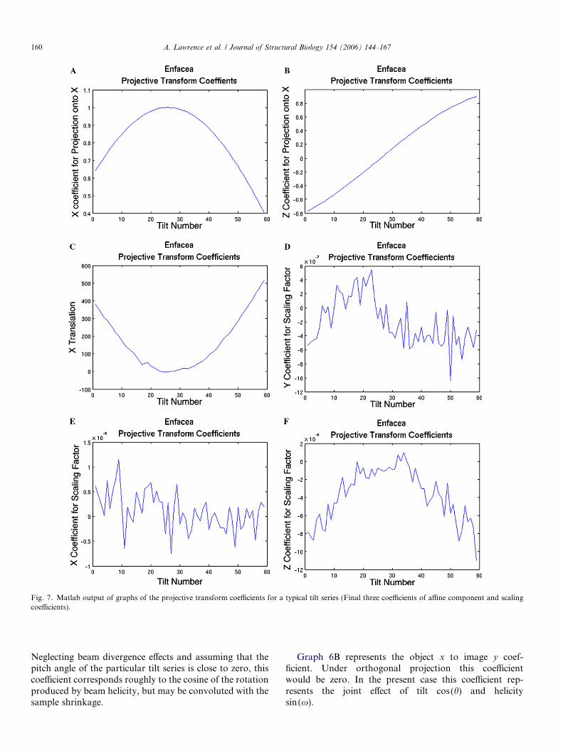
Fig. 7. Matlab output of graphs of the projective transform coefficients for a typical tilt series (Final three coefficients of affine component and scalingcoefficients).


Neglecting beam divergence effects and assuming that thepitch angle of the particular tilt series is close to zero, thiscoefficient corresponds roughly to the cosine of the rotationproduced by beam helicity, but may be convoluted with thesample shrinkage.

Graph 6B represents the object x to image y coef-ficient. Under orthogonal projection this coefficientwould be zero. In the present case this coefficient rep-resents the joint effect of tilt cos (h) and helicitysin (x).


Graph 6C represents the object z to image y coefficient.In the present case, this coefficient represents the jointeffects of tilt sin (h) and helicity sin (x).

Graph 6D represents the y translation. In the presentcase, this is a correction to the translations produced byIMOD xcorr alignment.

Graph 6E represents the object y to image x coefficient.In the case of orthogonal projection, this would be zero. Inthe present case this graph represents the effect of beamhelicity.

Graph 7A represents the x to x coefficient of the projec-tion. In this case, the dominant effect is the tilt angle cos (h).

Graph 7B represents the object z to image x coefficientof the projection. In this case, the dominant effect is dueto the tilt angle sin (h).

Graph 7C represents the x translation. The translationvalues represent the apparent x translation induced by tilt,which is in turn a function of the tilt angle and the positionof the tilt axis.

Graphs 7D–F represent the y, x, and z components ofthe scaling coefficient. In this case, the scaling coefficientis up to the noise level of the measurements, roughly y, zand tilt dependent. This indicates that the distortions arepseudo-projective (as described in Section 2.4) and thatbeam divergence effects are not significant in this tilt series.

Although our analysis of the significance of the trans-form coefficients is somewhat qualitative, it is clear thatuseful information may be obtained from the plots oftransform coefficients as a function of tilt. The plots pro-vide insight into the relationship between sample orienta-tion and beam geometry, which can reveal problems withmicroscope settings and/or tracking. Furthermore, thetransform coefficients are suggestive of alternative align-ment models. For example, our models may capture thebulk of the alignment information in fewer parameters.Such models could be more stable and robust, as well asavoiding the problems with singularities described inSection 5.1.

7.3. Flock house virus reconstruction

7.3.1. Sample preparation

Cultured Drosophila cells were prepared for electronmicroscopy according to Miller et al. (2001, 2003). For pur-poses of surveying the preservation quality of the samples,thin-sectioned material (�80-nm thick) was examined usinga JEOL 1200FX electron microscope. For three-dimen-sional reconstructions, sections from the samples were cutwith a thickness �300 nm from blocks exhibiting well-pre-served ultrastructure. These sections were stained for30 min in 2% aqueous uranyl acetate, followed by 30 minin lead salts. Fiducial cues consisting of 20 nm colloidalgold particles were deposited on both sides of the section.

7.3.2. Electron microscope imaging

A series of images was collected with a JEOL 4000EXintermediate-voltage electron microscope operated at

400 kV. The specimen was irradiated before initiating a tiltseries to limit anisotropic specimen thinning during imagecollection. Pre-irradiation in this manner subjected thespecimen to the steepest portion of the nonlinear shrinkageprofile before images were collected. The tilt series wasrecorded at angular increments of 2� from �64� to +66�about an axis perpendicular to the optical axis of themicroscope using a computer-controlled goniometer toincrement accurately the angular steps. The tilt series wasrecorded using a CCD camera with pixel size of1960 · 2560 (Fan et al., 2000). The microscope magnifica-tion was 40,000 giving a digitized scale of 0.55 nm per pixel.Each image represents a projection of density in the speci-men from a particular angle of view. The illumination washeld to near parallel beam conditions and optical densitymaintained constant by varying the exposure time to min-imize distortions in the projected image (Perkins et al.,1997).

7.3.3. Alignment

The IMOD software suite was used for cross-correlationalignment of the images in each tilt series followed by fidu-cial tracking (Kremer et al., 1996; Mastronarde, 1997). Acoarse translational and rotational alignment of each tiltseries was done first by cross-correlational alignment(IMOD xcorr) and subsequently by fine adjustmentsthrough the use of fiducial gold marks. In the IMOD align-ment, each image was aligned to the reference (nominalzero-tilt image) using 55 gold particles distributed overboth surfaces of the section. The IMOD program BEAD-TRACK was used to search for the position of each goldparticle on every image of the tilt series. The computer-gen-erated model of particle positions was examined with thebeadfixer utility from 3dmod and the incorrect positions,or failures to track a particle in some of the images, werecorrected. The TxBR utility TxBR_align_nonlinear wasused for fine tracking and alignment, using the IMODtracking as input. In particular, a projective transformmodel with quadratic corrections was employed for the finetracking. Both reconstructions utilized the same tracks.

7.3.4. Reconstruction

For the TxBR reconstruction, the first step was to per-form the pre-reconstruction step after tracking. In particu-lar, we performed simple rotations to level the tracks andto minimize filtering artifacts. The next step was to applythe Shepp–Logan filter to each tilt view, and then to calcu-late the precise projective transforms and quadratic correc-tions from object to the tilt view images. The tomographicreconstruction was generated by R-weighted backprojec-tion, using the TxBR software described above. We usedprojective maps with quadratic corrections calculated dur-ing the alignment as backprojection transformations. Forthe IMOD reconstruction, we used the standard procedurewith local alignments (25 patches). Fig. 8 shows a typicalimage from the tilt series. For the IMOD reconstruction,we used local alignments and the same fiducial data as

Fig. 8. Zero-tilt view of a Flock house virus series. Due to shadowing,structure of infected mitochondria is not clearly visible.


for the TxBR reconstruction, and the standard procedurefor reconstruction. The local alignment and reconstructionwas on 25 patches. Fig. 9A shows an x–y section which isas close as possible to the TxBR section, given minordifferences in orientation, while Fig. 9C shows an x–z sec-tion. Fig. 9B shows a central x–y section of the TxBRreconstruction and Fig. 9D shows a central x–z section ofthe TxBR reconstruction. Sharpness of detail is similar,while the TxBR reconstruction shows greatly reduced arti-facts in the x–z section.

Fig. 9. (A) A typical x–y section of a Flock house virus data set (FHV6) recoTxBR. (C) A typical x–z section of FHV6 reconstruction via IMOD. Note the rof the reconstruction via TxBR. Structure of infected mitochondria is cleaconsiderably more artifact. Details concerning production of the reconstructio

7.4. Quantum dots

7.4.1. Sample preparation

A mouse fibroblast cell, 10T 1/2, was transiently trans-fected with cDNA of DAKAP1a for 15 h. The cells werefixed with 4% paraformaldehyde at room temperature for1 min, and then transferred on ice for 9 min. The cells werethen treated with 0.1% Brij58 for 3 min on ice before treat-ed with antibodies. The primary antibody was purified(done by David Barraclough) with antigen RPP7 (an epi-tope of DAKAP1) and used at 18.5 lg/ml in 1% BSAand PBS. The Quantum dot 565 conjugated goat anti-rab-bit antibody was used as secondary antibody with 100·dilution in 1% BSA and PBS.


A double-tilt series was recorded on film on the JEOL4000 at 400 keV with angular increments of 2� from �60�to +60�. The grid was then rotated manually about 90�and a second tilt series was recorded of the region of inter-est using the same tilt angles. The microscope magnifica-tion was 20000. Each negative was scanned at 1800 dpigiving a pixel resolution of 0.64 nm.


Tracking and alignment were the same as for the FlockHouse virus data set. Eighty-five particles distributed overboth surfaces were used for alignment and corrections upto second order were employed. Reconstruction was accom-plished using both the IMOD and TxBR packages, as withthe Flock House virus data set. The TxBR reconstructionalso employed second-order corrections. Fig. 10 shows atypical EM image from the tilt series. Fig. 11A shows a cen-tral x–y section from the IMOD reconstruction (localoption), while Fig. 11C shows a central x–z section. Figs.

nstruction via IMOD. (B) A similar x–y section of the reconstruction viaeconstruction artifacts around the gold particles. (D) A similar x–z sectionrly visible in all reconstructions, but the IMOD reconstruction showsns are given in the text.

Fig. 10. Zero-tilt view from one of two tilt series data sets for the doubletilt quantum dot sample. The tilt axis is horizontal. The image is logtransformed to bring out details in darker areas. Due to shadowing, nano-particles around mitochondria are not clearly visible.


11B and D show corresponding sections from the TxBRreconstruction. Note that reconstruction quality is similar,while the TxBR reconstruction shows reduced artifacts.

7.5. Muscle tissue reconstruction

7.5.1. Preparation

Biological source is heart muscle from MLP knock outmouse. Sample was immersion fixed in 2% paraformalde-hyde and 2% glutaraldehyde in 0.15 M sodium cocadylatebuffer, and stained with 0.8% potassium ferrocyanide and2% osmium tetroxide in 0.15 M sodium cocadylate bufferfor 2 days at room temperature. Post staining, the samplewas incubated 30 min in 1% UA and 15 min in Sato lead.

Fig. 11. (A) A typical x–y section of double-tilt reconstruction of quantum doreconstruction via TxBR. (C) A typical x–z section of Qdot reconstruction via ITxBR. Note that sharpness of detail is similar in both reconstructions, while

The sample was then sectioned by 0.5 lm and subjectedto carbon evaporation and irradiation for stabilization.


The single tilt series was taken in the JEM4000 atNCMIR. Rotational increments were 2� over a total 120�rotation. The microscope was operated at 400 kV withmagnification; 8K. Images were taken on film and subse-quently digitized at 1.768 nm/pixel. Shutter speed was 2.8 s.


Tomographic tracking, alignment, and reconstructionwere performed as in the FHV series from 60 tilt views. For-ty-nine gold particles were used in the alignment. Alignmentand reconstruction for TxBR were performed using nonlin-ear quadratic, and alignment and reconstruction for IMODwere performed via local patches. Fig. 12 shows a typicalEM image from the tilt series. Fig. 13A shows a centralx–y section from the IMOD reconstruction, whileFig. 13C shows a central x–z section. Figs. 13B and D showcorresponding sections from the TxBR reconstruction. Notethat reconstruction sharpness and artifact levels are similar.

8. Findings

8.1. Bundle adjustment

The conjugate gradient method for computing theXYZ model along with the projective transforms hasproved to be quite stable, with rapid convergence to alocal minimum. We have observed problems only whenthe fiducial coordinates used as input to the process con-tain gross errors such as duplicate or missing points. Useof the projective model, on the other hand, carries somewell-known ambiguities, because the bundle adjustment

t sample (Qdot) via IMOD. (B) A similar x–y section of a double tilt QdotMOD. (D) A similar x–y section of double-tilt the Qdot reconstruction viaartifact level is reduced in the TxBR reconstruction.

Fig. 12. Zero-tilt view of muscle tissue series. Tilt axis is vertical. Due toshadowing, details of mitochondrial structure are not visible.


is well defined only up to a projective map. We havesome control over this, however, because the gold parti-cles used for fiducial marks are spherical, and significantdepartures from the expected geometry would be reflect-ed in distortions in the shape of the particles in thereconstruction. Nonlinearities are more difficult to con-trol. We have handled this problem by calculating thenonlinearities as corrections to the projective model, thusavoiding the intrinsic singularities of a combined model.Finally, we should note that average re-projection errorsare on the order of a pixel or less. Our re-projectionerrors are calculated as the square root of the meansquare distance between the original marks and the pro-jection of the calculated XYZ model as in formula(5.2.3). We note that the re-projection error decreasessubstantially when nonlinear corrections are employed.

Fig. 13. (A) A typical x–y section of muscle tissue sample (mlp-ko3) reconstrucA typical x–z section of the same IMOD reconstruction. (D) A similar x–z secstructure and general noise level are similar.

8.2. Reconstructions

The visual quality of our reconstructions is generallyexcellent. The examples offered above are typical. We rou-tinely obtain good contrast, with minimal artifacts and dis-tortion, as evidenced by the gold particles and otherfeatures of the reconstructions.

Although, we have depended upon visual inspection tojudge the quality of out reconstructions, we also have themore objective measure of the mean re-projection error.In general, the re-projection error at each of the trackedgold particles is on the order of a pixel or less. This impliesthat the images are well aligned in the neighborhood ofeach gold particle and, therefore, the backprojection is sim-ilarly accurate. The consequence of this is that up to the fil-tering errors, the backprojection will sum images correctly.

Our experience indicates that the transform methodhandles nonstandard geometric optics, optical distortion,and sample warping quite gracefully. We have been some-what limited in how far we can proceed in our measure-ment of geometric distortion, because faithful modelingof the geometry is dependent upon markers in the sample.Our methods depend upon deposited gold, and since thegold markers are limited to the surface, modeling volumet-ric distortion is similarly limited, unless the surface of thesample is rough or the sample is somewhat warped. In thiscase, variations in the z-dimension afford the opportunityto make nonlinear corrections in all three dimensions.When estimates in the z-dimension are available, recon-struction quality is improved.

8.3. Execution times

Although the pre-reconstruction processing is reason-ably fast, the backprojection itself is substantially slower

tion via IMOD. (B) A similar x–y section of reconstruction via TxBR. (C)tion of muscle tissue from TxBR reconstruction. Details of mitochondrial


than other implementations because various transformsmust be calculated repeatedly at each point of the recon-struction. We have been able to mitigate this somewhatby using differencing schemes in the calculation of thetransforms. In this way, we can perform reconstructionsusing projective and even nonlinear transforms for smallertilt series (on the order of 2k · 2k pixels/image), but largerimage series require another approach. Our algorithms areeasily programmed in parallel form, and we have observedthat inverse processing times scale nearly linearly with thenumber of processors. Accordingly, we have developed,tested, and fielded parallel versions of the reconstructionfor projective and quadratic forms of the reconstruction.

9. Discussion and conclusions

An objective of this work has been the development of amethod, which could adapt to the complexity of the elec-tron microscope as an optical instrument without havingto untangle each separate phenomenon and estimate itseffect on the process of image formation. The model ofimage formation as a geometrically nonlinear integraltransform from a three-dimensional object to a two-dimen-sional image has proved to be a simple, yet robust vehiclefor the inclusion of numerous optical effects. In effect, beameffects, sample warping, optical distortion, positioningerrors, and all the rest of the menagerie of problems maybe included in a lumped parameter model based on simplepolynomial functions. Advances in the precision of stagesand stability of optics in modern transmission EM’s areleading to improved results with electron tomography,but even small errors of a fraction of a percent can producequite unwelcome degradation of reconstruction quality,especially with large images.

Although our method of handling the geometric prob-lems of tomographic reconstruction from EM imagesappears to be quite effective and appears to give improve-ments in reconstruction quality, other problems remain.We have already devoted some attention to one; the prob-lem of pre-filtering. A second problem is implicit in our dis-cussion; the growth in the required number of fiducialmarks as the degree (and accuracy) of the polynomialapproximations is increased. Finally, no discussion of anew method would be complete without some attentionto the problem of verification.

9.1. Pre-filtering

Our pre-filtering algorithm is based on the assumptionthat the paths of the electrons stay in planes perpendicularto the rotation axis. Although this is nearly true, even withremapping, the backprojection image of a line in imagespace forms a curvilinear region in the object space. Moreprecisely, if the images are aligned so that all the fiducialtracks are as parallel as possible to the x-axis, then theunion of all the backprojection images of a track underthe projection transforms constitutes a curvilinear surface

in the object. This implies that the reconstruction problemdoes not decompose into the problem of reconstructionalong two-dimensional planes, so a simple one-dimensionalfilter is not correct. We should note that even when thegeometry is purely projective, as in cone-beam reconstruc-tion, the pre-filter must be more complex than the simpleone-dimensional Shepp–Logan filter that we employ(Grangeat, 1991; Katsevich, 2002; Tuy, 1983; Ye andWang, 2005). On one hand, the departures from the simplecase are small (on the order of a few pixels), so, the errorwe introduce by treating the problem as an orthogonal pro-jection is also small. However, on the other hand, weexpect that a filter corresponding to the true geometryshould give better reconstructions.

9.2. Polynomial approximations

Eleven coefficients are required for a generalized pro-jective map from three-dimensional space to two-dimen-sional space. If quadratic corrections are added, thisnumber increases to 23, and if cubic corrections areincluded, the number increases to 41, and so forth. Forstatistical accuracy, we should have at least two or threefiducial marks for each coefficient to be determined. Usingdeposited gold to establish fiducial marks is time-consum-ing, and because the gold particles contribute artifacts oftheir own, large numbers of gold particles can degradereconstruction quality. Alternative methods are requiredto establish the projections. One promising approach isto apply the method of occluded contours (Boyer andBergier, 1996; Forsyth, 1996; Kang et al., 2001). The basicidea is to identify contours in the tilt images and approx-imate them as curves, which are defined by polynomials.At this point, basic theorems in algebraic geometry canbe applied to determine surfaces in three dimensions,which project to the contours in the tilt images. In partic-ular, a contour in a tilt image is a projection of a curveembedded in a surface in the object and the electron tra-jectories are tangent to the surface precisely at the pointsof the curve. All of these conditions translate to algebraicexpressions for the surface and the projection maps whichcan be calculated by techniques very similar to the bundleadjustment techniques we describe in this paper. In fact,the method of occluded contours can be regarded as ageneralization of methods, which depend upon configura-tions of fiducial marks.

We must note that biological objects are generally richin membranes, which form surfaces enclosing well-definedvolumes. These membranes generally stain quite clearly,and because of the density gradients, project to clearly vis-ible contours in electron microscope images (Radermacherand Frank, 1984). Because of the large density gradients inthe neighborhood of stained membranes, the projectedcontours must reflect curves at which the electron trajecto-ries are tangent to the membrane. Using the geometric fea-tures of the object, itself, to determine the projection mapswould obviate the use of deposited particles.


9.3. Verification

Phantoms are commonly used to verify algorithms usedin image processing. Unfortunately, what is usually missingin use of a phantom is a solid justification of the accuracyof the model implicit in the phantom. A phantom mustprovide an accurate model of both the object itself, andthe imaging process in order that we can make strong infer-ences about the correspondence between the tomographicreconstruction and the composition of the object andwhether our reconstruction provides a good model of theobject. For this reason, we have directed our attentiontoward objects that seem to be well characterized, andabout which there is general agreement concerning the ori-ginal composition and how that composition should bereflected in a reconstruction. This is the major reason wehave concentrated our attention on gold particles. Methodsthat give solid, regular ball-shaped reconstructions of goldparticles with minimal surrounding artifacts should alsogive superior reconstructions of other structures. A secondform of verification is that empty spaces should be free ofartifacts from surrounding structures (Herman and Tuy,1985). Unfortunately, thin slices, which occupy the wholeelectron beam, are not good candidates for analysis, eventhough the space above and below the slice should bereconstructed without structure. There are several reasonsfor this. First, a range of about 60� of the high tilt anglesare inevitably missing, so there is no way to completelyclear the artifacts from the space above and below theobject without running into the essential singularities ofthe transform from object to the space of tilt views. Second,because of the interference from the surrounding sampleholder, additional information is missing from the highertilts. Because reconstruction in three-dimensional space isintrinsically a nonlocal process, attaining the objective ofreconstruction of empty space as empty is further stymied.One way of avoiding these difficulties is to suspend a nar-row object at one or both ends, thus surrounding the objectby 360� of empty space, and enabling a higher range oftilts. This geometry makes it much easier to impose addi-tional numerical conditions on the reconstruction, whichin effect force the reconstruction of empty space as empty.Such conditions can, for example, be imposed on an itera-tive reconstruction, which is based on the more accurateprojection maps we derive.

In conclusion, we believe that the transform methodoffers substantial improvements in reconstruction quality,and that the techniques we have developed can be extendedin directions, which promise significant results.

Acknowledgments

The authors thank Professor Jose Maria Carazo ofAutonoma University, Madrid, for his encouragement ofthis work and his careful reading and criticism of earlydrafts of the manuscript. The authors further thank Drs.Kyoshi Hama, Tatsuo Arii, and David Mastronarde for

helping to inspire this work. We are especially grateful toDr. Mastronarde for his detailed explanations of the mod-ules of the IMOD package that were foundational to thiseffort. We also express our appreciation to Ben Kopekand Paul Ahlquist for providing the Flock House Virusdata, Takeharu Hoyashi for providing the heart muscledata, Tom Deerinck and Frank Ma for providing thequantum dot data, Mason Mackey for his efforts in obtain-ing much of the EM data, and Masako Terada for heruntiring efforts in testing all of the components of theTxBR software package and Alex Kulungowski for hishelp in performing the labor associated with producingthe reconstructions. Last, but not least, many of the recon-structions would not be done in a timely manner withoutthe parallel version of the backprojection code providedby Amit Majumdar of the San Diego Supercomputer Cen-ter. This work is supported by the National Institutes ofHealth (NIH) Biomedical Technology Resource CentersProgram of the National Center for Research Resources(NCRR) through Grant Numbers P41 RR04050 (for theNational Center for Microscopy and Imaging or Research(NCMIR)) and P41 RR008605 (for the National Biomed-ical Computation Resource (NBCR)).

References

Agar, A.W., 1974. Principles and Practice of Electron MicroscopeOperation. American Elsevier Publishing, New York.

Aikens, R.S., Agard, D.A., Sedat, J.W., 1989. Solid state imagers formicroscopy. Methods Cell Biol. 29, 291.

Anderson, E., Bai, Z., Bischof, C., Blackford, S., Demmel, J., Dongarra,J., Du Croz, J., Greenbaum, A., Hammarling, S., McKenney, A.,Sorenson, D., 1999. LAPACK User’s Guide. SIAM, Philadelphia.

Arii, T., Hama, K., 1987. Method of extracting three-dimensionalinformation from HVTEM stereo images of biological materials. J.Electron Microsc. (Tokyo) 36 (4), 177–195.

Baldwin, P.R., Pawel, A., Penczek, P., 2005. Estimating alignment errorsin sets of 2-D images. J. Struct. Biol. 150, 211–225.

Beylkin, G., 1984. The inversion problem and applications of the generalizedradon transform. Commun. Pure Appl. Math. 37, 579–599.

Bouwer, J.C., Mackey, M.R., Lawrence, A., Deerinck, T.J., Jones, Y.Z.,Terada, M., Martone, M.E., Peltier, S., Ellisman, M.H., 2004.Automated most-probable loss tomography of thick selectively stainedbiological specimens with quantitative measurement of resolutionimprovement. J. Struct. Biol. 148 (3), 297–306.

Boyer, E., Bergier, M.-O., 1996. 3D surface reconstruction using occludedcontours. Int. J. Comput. Vision 22 (3), 219–233.

Brandt, S., Heikkonen, J., Engelhardt, P., 2001a. Automatic alignment oftransmission electron microscope tilt series without fiducial markers. J.Struct. Biol. 136 (3), 201–213.

Brandt, S., Heikkonen, J., Engelhardt, P., 2001b. Multiphase method forautomatic alignment of transmission electron microscope images usingmarkers. J. Struct. Biol. 133 (1), 10–22.

Chapman, J.N., Craven, A.J., Scott, C.P., 1989. Electron detection in theanalytical electron microscope. Ultramicroscopy 28, 108.

Daberkow, I., Herrmann, K.-H., Liu, L., Rau, W.D., Tietz, H., 1996.Development and performance of a fast fiber-plate coupled CCDcamera at medium energy and image processing system for electronholography. Ultramicroscopy 75, 215–233.

Defrise, M., 1995. A factorization method for the 3D X-ray transform.Inverse Problems 11, 983–994.

Denysuk, A.S., 1994. Inversion of the generalized radon transform. Am.Math. Soc. Transl. 162 (2), 19–32.


Downing, K.H., Hendrickson, F.M., 1999. Performance of a 2k CCDcamera designed for electron crystallography at 400 kV. Ultramicros-copy 75 (4), 215–233.

Ehrenpreis, L., 2003. The Universality of the Radon Transform. OxfordUniversity Press, New York.

Fan, G.Y., Ellisman, M.H., 1993. High-sensitivity lens-coupled slow-scanCCD camera for transmission electron microscopy. Ultramicroscopy52 (1), 21–29.

Fan, G.Y., Ellisman, M.H., 2000. Digital imaging in transmission electronmicroscopy. J. Microsc. 200 (Pt. 1), 1–13.

Fan, G.Y., Peltier, S., Lamont, S., Dunkelberger, D.G., Burke, B.E.,Ellisman, M.H., 2000. Multiport-readout frame-transfer 5 megapixelCCD imaging system for TEM applications. Ultramicroscopy 84 (1–2),75–84.

Fan, G.Y., Young, S.J., Miller, P., Ellisman, M.H., 1995. Conditions forelectron tomographic data acquisition. J. Electron Microsc. (Tokyo)44 (1), 15–21.

Faugeras, O., Luong, Quang-Tuan, 2001. The Geometry of MultipleImages. MIT Press, Cambridge, MA.

Forsyth, D.A., 1996. Recognizing algebraic surfaces from their outlines.Int. J. Comput. Vision 18, 21–40.

Frank, J., 1992. Electron Tomography: Three-dimensional Imaging withthe Transmission Electron Microscope. Plenum Press, New York.

Frank, J., Chiu, W., Henderson, R., 1993. Flopping polypeptide chainsand Suleika’s subtle imperfections: analysis of variations in theelectron micrograph of a purple membrane crystal. Ultramicroscopy49, 387–396.

Grangeat, P., 1991. Mathematical framework of cone beam 3D recon-struction via the first derivative of the Radon transform. MathematicalMethods in Tomography. In: Herman, G.T., Louis, A.K., Natterer,F., (Eds.), Lect. Notes Math., 1497, 66–97.

Gropp, W., Lusk, E., Skjellum, A., 1999. Using MPI Portable ParallelProgramming with the Message-Passing Interface. The MIT Press,Cambridge, MA.

Guillemin, V., 1985. On some results of Gelfand in integral geometry,Pseudodifferential operators and applications. (Notre Dame, Ind.,1984), AMS Proc. Symposia in Pure Math. 43, 149–155.

Hartshorne, R., 1977. Algebraic Geometry. Springer Verlag, Berlin, pp.47–54.

Herman, G.T., Tuy, H.K., 1985. The radon transform in the space ofdistributions with compact support. In: Sabatier, P.C., Hilger, A.(Eds.), Basic Methods of Tomography and Inverse Problems. Bristol.

Herrmann, K.-H., Sikeler, R., 1995. Low-energy electron image convertersfor high resolution slow-scan CCD sensor. Optik 98, 119.

Heyden, A., Astrom, K., 1997. Euclidean reconstruction from almostuncalibrated cameras. In: SSAB Symposium, Stockholm.

deHoop, M.V., 2003. Microlocal analysis of seismic inverse scattering. In:Uhlmann, G. (Ed.), Inside Out. Cambridge University Press, Cam-bridge, pp. 219–298.

Kang, K., Tarel, J.-P., Fishman, R., Cooper, D., 2001. A linear dual-spaceapproach to 3D surface reconstruction from occluding contours usingalgebraic surfaces. IEEE Int. Conf. Comput. Vision 1, 198–204.

Katsevich, A., 2002. Microlocal analysis of an FBP algorithm fortruncated spiral cone beam data. J. Fourier Anal. Appl. 8, 407–426.

Kremer, J.R., Mastronarde, D.N., McIntosh, J.R., 1996. Computervisualization of three-dimensional image data using IMOD. J. Struct.Biol. 116 (1), 71–76.

Krivanek, O.L., Mooney, P.E., Fan, G.Y., 1991. Slow-scan CCD camerasin transmission electron microscopy. Inst. Phys. Conf. Ser. 119, 523.

Kujawa, S., Krahl, D., 1992. Performance of a low-noise CCDcamera adapted to a transmission electron microscope. Ultramicros-copy 46, 395.

Martone, M.E., Gupta, A., Wong, M., Qian, X., Sosinsky, G., Ludascher,B., Ellisman, M.H., 2002a. A cell-centered database for electrontomographic data. J. Struct. Biol. 138 (1–2), 145–155.

Martone, M.E., Gupta, A., Ludaescher, B., Zaslavski, I., Ellisman, M.H.,2002. Federation of brain data using knowledge guided mediation. In:Kotter, R. (Ed.), Neuroscience Databases: A Practical Guide. Norwell, MA.

Mastronarde, D.N., 1997. Dual-axis tomography: an approach withalignment methods that preserve resolution. J. Struct. Biol. 120 (3),343–352.

Mathworks, t., 2002. Matlab the Language of Technical Computing,Using Matlab Version 6. The MathWorks, Natik, MA.

Mathworks, t., 2002. Optimization Toolbox for Use with Matlab, UserGuide Version 2. The Mathworks, Natik, MA.

Miller, D.J., Schwartz, M.D., Ahlquist, P., 2001. Flock house virus RNAreplicates on outer mitochondrial membranes in Drosophila cells. J.Virol. 75, 11664–11676.

Miller, D.J., Schwartz, M.D., Dye, B.T., Ahlquist, P., 2003. Engineeredretargeting of viral RNA replication complexes to an alternativeintracellular membrane. J. Virol. 77, 12193–12202.

Mukhometov, R.G., 1975a. Inverse kinematic problem of seismic on theplane, Math. Problems of Geophysics. Akad. Nauk. SSSR, Sibirsk.Otdel., Vychisl. Tsentr, Novosibirsk 6, 243–252.

Mukhometov, R.G., 1975b. On the problem of integral geometry, Math.Problems of Geophysics. Akad. Nauk. SSSR, Sibirsk. Otdel., Vychisl.Tsentr, Novosibirsk 6, 212–242.

Natterer, F., Wubbeling, F., 2001. Mathematical Methods in ImageReconstruction. Society for Industrial and Applied Mathematics,Philadelphia, PA.

Penczek, P., Marko, M., Buttle, K., Frank, J., 1995. Double-tilt electrontomography. Ultramicroscopy 60, 393–410.

Perkins, G.A., Renken, C.W., Song, J.Y., Frey, T.G., Young, S.J.,Lamont, S., Martone, M.E., Lindsey, S., Ellisman, M.H., 1997.Electron tomography of large, multicomponent biological structures.J. Struct. Biol. 120 (3), 219–227.

Popov, D.A., 2001. The generalized radon transform on the plane, theinverse transform, and the Cavalieri conditions. Funct. Anal. Appl. 35,270–283.

Quinto, E.T., 1993. Singularities of the X-ray transform andlimited data tomography in R3. SIAM J. Math. Anal. 24,1215–1225.

Radermacher, M., Frank, J., 1984. Representation of three-dimensionallyreconstructed objects in electron microscopy by surfaces of equaldensity. J. Microsc. 136 (Pt. 1), 77–85.

Reimer, L., 1993. Transmission Electron Microscopy: Physics of ImageFormation and Mirooanalysis. Springer, Berlin.

Roberts, P.T.E., Chapman, J.N., Mac Leod, A.M., 1982. A CCD-basedimage recording system for the CTEM. Ultramicroscopy 8, 385.

Romanov, V.G., 1974. Integral Geometry and Inverse Problems forHyperbolic Equations. Springer-Verlag, Berlin.

Ruska, E., 1986. The development of the electron microscope and ofelectron microscopy. Nobel Lecture.

Semple, I.G., Kneebone, G.T., 1998. Algebraic Projective Geometry.Clarendon Press, Oxford.

Sharafutdinof, V.A., 1999. Ray Transforms on Riemannian Manifolds,Lecture Notes. University of Washington, Seattle.

Soto, G.E., Young, S.J., Martone, M.E., Deerinck, T.J., Lamont, S.,Carragher, B.O., Hama, K., Ellisman, M.H., 1994. Serial sectionelectron tomography: a method for three-dimensional reconstructionof large structures. Neuroimage 1 (3), 230–243.

Spence, J.C.H., Zuo, J.M., 1998. Large dynamic range, parallel detectionsystem for electron diffraction and imaging. Rev. Sci. Instrum. 59 (9),2102.

Triggs, B., McLauchlan, P., Hartley, R., Fitzgibbon, A., 2000. Bundleadjustment—a modern synthesis. In: Triggs, A., Zisserman, A.,Szeliski, R. (Eds.), Vision Algorithms: Theory and Practice. Spring-er-Verlag, Berlin.

Tsuna, K., Harada, Y., 1981. Minimisation of radial and spiral distortionin electron microscopy through the use of a triple pole-piece lens. J.Phys. E: Sci. Instrum. (14), 313–320.

Tuy, H.K., 1983. An inversion formula for cone-beam reconstruction.SIAM J. Appl. Math. 43, 546–552.

Ye, Y., Wang, G., 2005. Filtered backprojection formula for exact imagereconstruction from cone-beam data along a general scanning curve.Med. Phys. 32, 42–48.

transform-based backprojection for volume reconstruction of large format electron microscope tilt...

Documents