transaction level modeling for noc and soc...
TRANSCRIPT
TRANSACTION LEVEL MODELING FOR NOC AND SOC
By
Amr Ahmed Hany Mohamed
A Thesis Submitted to the
Faculty of Engineering at Cairo University
in Partial Fulfillment of the
Requirements for the Degree of
MASTER OF SCIENCE
in
Electronics and Communications Engineering
FACULTY OF ENGINEERING, CAIRO UNIVERSITY
GIZA, EGYPT
2015
TRANSACTION LEVEL MODELING FOR NOC AND SOC
By
Amr Ahmed Hany Mohamed
A Thesis Submitted to the
Faculty of Engineering at Cairo University
in Partial Fulfillment of the
Requirements for the Degree of
MASTER OF SCIENCE
in
Electronics and Communications Engineering
Under the Supervision of
Dr. Hossam A. H. Fahmy
……………………………….
Dr. Magdy A. El-Moursy
……………………………….
Associate Professor
Communications and Electronics
Department
Faculty of Engineering, Cairo University
Associate Professor
Microelectronics Department
Electronics, Research Institute, Cairo, Egypt
FACULTY OF ENGINEERING, CAIRO UNIVERSITY
GIZA, EGYPT
2015

TRANSACTION LEVEL MODELING FOR NOC AND SOC
By
Amr Ahmed Hany Mohamed
A Thesis Submitted to the
Faculty of Engineering at Cairo University
in Partial Fulfillment of the
Requirements for the Degree of
MASTER OF SCIENCE
in
Electronics and Communications and Engineering
Approved by the
Examining Committee
____________________________
Dr. Hossam A. H. Fahmy, Thesis Main Advisor
____________________________
Dr. Magdy A. El-Moursy, Member, Microelectronics department,
Electronics Research Institute
____________________________
Dr. Tamer Farid El-Batt, Internal Examiner
____________________________
Prof. Dr. Mohamed Amin Dessouky, External Examiner, Faculty of
Engineering, Ain Shams University
FACULTY OF ENGINEERING, CAIRO UNIVERSITY
GIZA, EGYPT
2015
Engineer’s Name: Amr Ahmed Hany Mohamed
Date of Birth: 21/08/1987
Nationality: Egyptian
E-mail: [email protected]
Phone: 01227406044
Address: 16 Gad Eid St., Dokki, Giza
Registration Date: 01/10/2009
Awarding Date: …./…./……..
Degree: Master of Science
Department: Electronics and Communications Engineering
Supervisors:
Dr. Hossam A. H. Fahmy
Dr. Magdy A. El-Moursy, Microelectronics department,
Electronics Research Institute
Examiners:
Dr. Hossam A. H. Fahmy
Dr. Magdy A. El-Moursy, Microelectronics department,
Electronics Research Institute
Dr. Tamer Farid El-Batt
Prof. Dr. Mohammed Amin Dessouky, Faculty of
Engineering, Ain Shams University
Title of Thesis:
Transaction Level Modeling for NoC and SoC
Key Words:
Transaction Level Modeling; Network on Chip; System on Chip; Traffic Generation
Summary:
Transaction level model for Network on Chip (NoC) router is used to implement NoC
and compare it to System on Chip (SoC) bus model. Performance evaluation is
presented for both systems using different traffic loads and patterns along with different
network sizes.
Insert photo here

i
Acknowledgments
I would like to thank my supervisors Dr. Magdy El-Moursy and Dr. Hossam
Fahmy for giving me the opportunity to work on my master thesis in their research
group. I want to thank them for their patient guide, from which I have learnt the
fundamental knowledge of how to research. I would also like to thank my parents and
my wife. Without them I would not be able neither to attend the master program nor to
finish the master thesis.

ii
Dedication
To my wife, my mother, my father, my sister, my grandmother, and my baby girl
Mariam.
iii
Table of Contents
ACKNOWLEDGMENTS ............................................................................................. I
DEDICATION ............................................................................................................... II
TABLE OF CONTENTS ............................................................................................ III
LIST OF TABLES .......................................................................................................VI
LIST OF FIGURES ................................................................................................... VII
NOMENCLATURE .....................................................................................................IX
ABSTRACT ................................................................................................................... X
CHAPTER 1 : INTRODUCTION AND BACKGROUND ...................................... 11
1.1. INTRODUCTION .................................................................................. 11
1.2. CONTRIBUTION .................................................................................. 11
1.3. ORGANIZATION OF THE THESIS ........................................................... 12
1.4. NOC INTRODUCTION .......................................................................... 12
1.4.1. Interconnect Network Architectures ..................................................... 12
1.4.2. Flow Control Units................................................................................ 12
1.4.3. Switching Techniques ........................................................................... 13
1.4.4. Router Architecture ............................................................................... 13
1.4.5. NoC Topologies .................................................................................... 14
1.5. ROUTING ALGORITHMS ...................................................................... 15
1.5.1. Source and Distributed Routing ............................................................ 15
1.5.2. Deterministic and Adaptive Routing ..................................................... 16
1.5.3. Routing Algorithms Examples .............................................................. 16
1.6. ARBITRATION .................................................................................... 20
1.7. RELATED WORK ................................................................................ 22
1.7.1. NoC Comparison................................................................................... 22
1.7.2. Multi-synchronous vs. Asynchronous ................................................... 22
1.7.3. QoS Communication Schemes .............................................................. 23
1.7.4. NoC Router Architecture ...................................................................... 24
1.7.5. Comparison of Æthereal NoC and Bus ................................................. 25
1.7.6. Bus Enhanced NoC ............................................................................... 25
1.7.7. Bus and NoC Comparison ..................................................................... 26
1.8. CONCLUSION ...................................................................................... 27
CHAPTER 2 : ROUTER AND BUS MODELS ........................................................ 28
2.1. INTRODUCTION .................................................................................. 28
2.1.1. Modeling Levels ................................................................................... 28
2.1.2. Transaction Level Modeling ................................................................. 29
2.1.3. Modeling for High Performance ........................................................... 30
2.1.4. The Scalable Model Approach .............................................................. 30
2.2. ROUTER FEATURES ............................................................................ 31
iv
2.3. MODELING TIMING FOR THE ROUTER: ............................................... 32
2.4. MODELING POWER ............................................................................. 33
2.5. BUS MODEL ....................................................................................... 34
2.5.1. AMBA Introduction: ............................................................................. 34
2.5.2. AMBA AHB ......................................................................................... 35
2.5.3. Modeling Timing for AHB Bus ............................................................ 36
2.5.4. Bus Arbitration ...................................................................................... 36
2.6. CONCLUSION ...................................................................................... 37
CHAPTER 3 : TRAFFIC GENERATION ................................................................ 38
3.1.1. Introduction ........................................................................................... 38
3.2. TRAFFIC KINDS .................................................................................. 38
3.3. EMULATING IP COMMUNICATION BEHAVIOR .................................... 38
3.4. TRAFFIC GENERATION PARAMETERS ................................................. 39
3.5. CONFIGURABLE TRAFFIC GENERATOR ............................................... 40
3.6. LITERATURE SURVEY ......................................................................... 41
3.6.1. NoC Simulator ...................................................................................... 41
3.6.2. NoC Traffic Suite .................................................................................. 41
3.6.3. NoC Framework .................................................................................... 42
3.6.4. Statistical Traffic Model ....................................................................... 43
3.6.5. Effect of Traffic Localization: .............................................................. 43
3.6.6. Traffic Models for Benchmarking ........................................................ 44
3.7. PERFORMANCE EVALUATION ............................................................. 44
3.7.1. Performance Metrics ............................................................................. 45
3.8. CONCLUSION ...................................................................................... 45
CHAPTER 4 : SIMULATION AND RESULTS ....................................................... 46
4.1. INTRODUCTION .................................................................................. 46
4.2. NOC SIMULATION .............................................................................. 46
4.2.1. NoC Simulation Phases ......................................................................... 47
4.3. SOC SIMULATION .............................................................................. 48
4.4. TRAFFIC GENERATION ....................................................................... 48
4.5. 2X2 RESULTS ..................................................................................... 49
4.5.1. Throughput ............................................................................................ 49
4.5.2. Latency .................................................................................................. 53
4.5.3. Number of Hops .................................................................................... 59
4.5.4. Power .................................................................................................... 60
4.6. 3X3 RESULTS: .................................................................................... 66
4.6.1. Throughput ............................................................................................ 68
4.6.2. Latency .................................................................................................. 69
4.6.3. Number of Hops .................................................................................... 71
4.6.4. Power .................................................................................................... 72
4.7. 4X4 RESULTS: .................................................................................... 74
4.7.1. Throughput ............................................................................................ 75
4.7.2. Latency .................................................................................................. 76
4.7.3. Number of Hops .................................................................................... 77

v
4.7.4. Power .................................................................................................... 78
DISCUSSION AND CONCLUSIONS ....................................................................... 80
FUTURE WORK ......................................................................................................... 81
REFERENCES ............................................................................................................. 82
APPENDIX A: SYSTEMC CODE FOR ROUTER MODEL ................................. 86
APPENDIX B: SYSTEMC CODE FOR CPU MODEL........................................... 88
APPENDIX C: C CODE FOR TRAFFIC GENERATION ..................................... 94
PUBLICATION ............................................................................................................ 95

vi
List of Tables
Table 4.1: Comparison of Throughput and Power Curves ............................................. 66
Table 4.2: Comparison of Throughput and Power Slopes ............................................. 74 Table 4.3: Comparison of Throughput and Power Slopes ............................................. 79

vii
List of Figures
Figure 1.1: Router state diagram .................................................................................... 14
Figure 1.2: (a) 2D Mesh, (b) Ring, (c) Spidergon, (d) Crossbar .................................... 15 Figure 1.3: NoC architectures......................................................................................... 15 Figure 1.4: Example of region definition ....................................................................... 19 Figure 1.5: ASPRA Design Methodology ...................................................................... 20 Figure 1.6: (a) Centralized arbitration; (b) Distributed arbitration................................. 21
Figure 1.7: Multi-synchronous system ........................................................................... 23 Figure 1.8: (a) Connection-oriented router (b) Connectionless-oriented router ............. 24
Figure 1.9: Router Architecture ...................................................................................... 24
Figure 1.10: BENoC ....................................................................................................... 26 Figure 1.11: Spidernet NoC ............................................................................................ 27 Figure 2.1: Blocking and non-blocking interfaces [30].................................................. 30 Figure 2.2: PVT model structure [30] ............................................................................ 31 Figure 2.3: Router model ................................................................................................ 32
Figure 2.4: Sequential policy [30] .................................................................................. 33
Figure 2.5: 2x2 mesh network ........................................................................................ 34 Figure 2.6: Typical AMBA system ................................................................................ 35
Figure 2.7: N-layer AHB system [25] ............................................................................ 36 Figure 2.8: Pipeline policy [30] ...................................................................................... 36 Figure 2.9: Bus model [30] ............................................................................................. 37
Figure 3.1: Emulating real traffic ................................................................................... 39
Figure 3.2: Traffic configuration parameters [39] .......................................................... 39 Figure 3.3: Complement traffic pattern [41] .................................................................. 40 Figure 3.4: Traffic generation methodology .................................................................. 42
Figure 3.5: 3-tuple traffic model .................................................................................... 43 Figure 3.6: (a) External evaluation; (b) Internal evaluation ........................................... 44
Figure 4.1: 2x2 NoC ....................................................................................................... 47 Figure 4.2: 2x2 SoC ........................................................................................................ 48 Figure 4.3: 2x2 Routers Coordinates .............................................................................. 49 Figure 4.4: Throughput for different active cores .......................................................... 50
Figure 4.5: Normalized throughput for different traffic loads ....................................... 51 Figure 4.6: Throughput percentage change (Constant Bit Rate) .................................... 51
Figure 4.7: Normalized throughput for Normal distribution traffic pattern ................... 52 Figure 4.8: Throughput percentage change (Normal) .................................................... 52 Figure 4.9: Normalized throughput for Poisson distribution traffic pattern ................... 53 Figure 4.10: Throughput percentage change (Poisson) .................................................. 53 Figure 4.11: Latency distribution for NoC with constant bit rate .................................. 54
Figure 4.12: Average latency for NoC ........................................................................... 54 Figure 4.13: SoC Latency ............................................................................................... 55 Figure 4.14: SoC latency distribution (Normal) ............................................................. 55 Figure 4.15: NoC Latency distribution (Normal) ........................................................... 56 Figure 4.16: SoC Latency distribution (Poisson) ........................................................... 56
Figure 4.17: NoC Latency distribution (Poisson)........................................................... 57 Figure 4.18: Average NoC latency (Normal) ................................................................. 57
Figure 4.19: Average SoC latency (Normal) .................................................................. 58 Figure 4.20: Average NoC latency (Poisson) ................................................................. 58
viii
Figure 4.21: Average SoC latency (Poisson) ................................................................. 59 Figure 4.22: Number of hops for 2x2 NoC (Constant Bit Rate) .................................... 59 Figure 4.23: Number of hops for 2x2 NoC (Normal) .................................................... 60 Figure 4.24: Number of hops for 2x2 NoC (Poisson) .................................................... 60 Figure 4.25: Power comparison of NoC vs. SoC (Constant Bit Rate) ........................... 61
Figure 4.26: Power comparison of NoC vs. SoC (Normal) ........................................... 62 Figure 4.27: Power comparison of NoC vs. SoC (Poisson) ........................................... 62 Figure 4.28: Normalized Throughput and Power (Constant Bit Rate) ........................... 63 Figure 4.29: Normalized Throughput and Power (Normal) ........................................... 63 Figure 4.30: Normalized Throughput and Power (Poisson) ........................................... 64
Figure 4.31: Power Percentage Change (Constant Bit Rate) ......................................... 64 Figure 4.32: Power Percentage Change (Normal) .......................................................... 65
Figure 4.33: Power Percentage Change (Poisson) ......................................................... 65 Figure 4.34: Line of Best Fit Example ........................................................................... 66 Figure 4.35: 3x3 routers coordinates .............................................................................. 66 Figure 4.36: 3x3 NoC ..................................................................................................... 67 Figure 4.37: 3x3 SoC ...................................................................................................... 68
Figure 4.38: Normalized throughput (Normal) .............................................................. 68 Figure 4.39: Throughput Percentage Change (Normal) ................................................. 69
Figure 4.40: SoC latency distribution ............................................................................. 69 Figure 4.41: NoC latency distribution ............................................................................ 70
Figure 4.42: Average SoC Latency ................................................................................ 70 Figure 4.43: Average NoC latency ................................................................................. 71 Figure 4.44: 3x3 NoC number of hops ........................................................................... 71
Figure 4.45: Average number of hops for 3x3 NoC ....................................................... 72
Figure 4.46: Normalized Power for 3x3 NoC and SoC .................................................. 72 Figure 4.47: Power percentage change ........................................................................... 73 Figure 4.48: Normalized Throughput and power ........................................................... 73
Figure 4.49: 4x4 router coordinates................................................................................ 74 Figure 4.50: Normalized Throughput (Normal) ............................................................. 75
Figure 4.51: Throughput Percentage Change (Normal) ................................................. 75 Figure 4.52: SoC latency distribution ............................................................................. 76 Figure 4.53: NoC latency distribution ............................................................................ 76
Figure 4.54: 4x4 NoC number of hops ........................................................................... 77 Figure 4.55: Average number of hops for 4x4 NoC ....................................................... 77
Figure 4.56: Normalized Power for 4x4 SoC and NoC.................................................. 78
Figure 4.57: Power percentage change ........................................................................... 78
Figure 4.58: Normalized Throughput and power ........................................................... 79

ix
Nomenclature
IP Intellectual Property
NoC Network on Chip
SoC System on Chip
TLM Transaction Level Modeling
x
Abstract
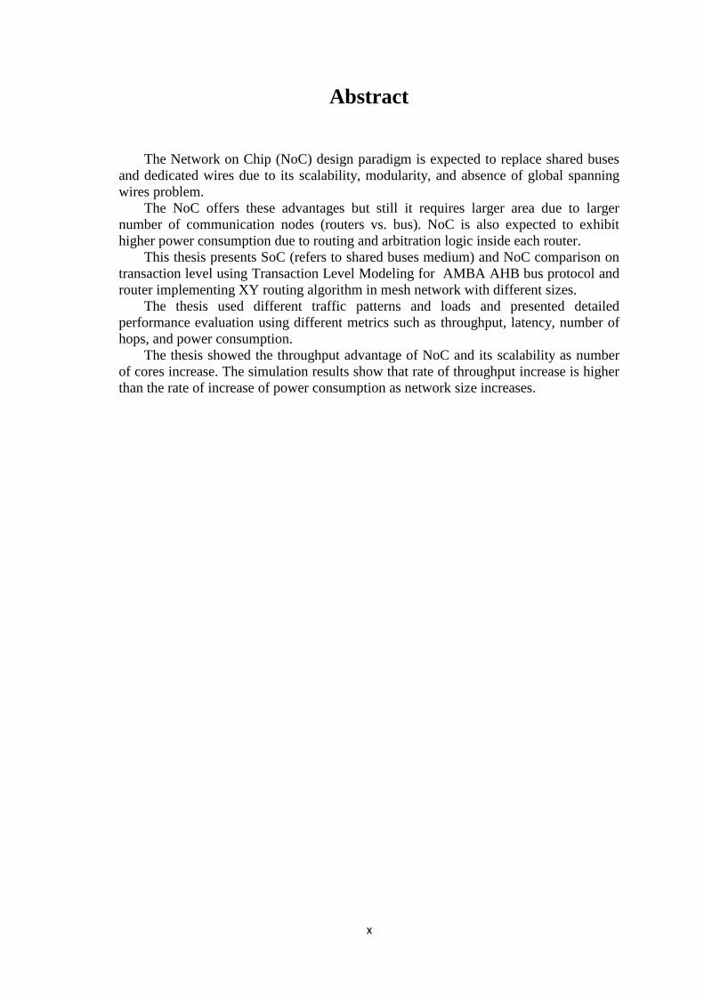
The Network on Chip (NoC) design paradigm is expected to replace shared buses
and dedicated wires due to its scalability, modularity, and absence of global spanning
wires problem.
The NoC offers these advantages but still it requires larger area due to larger
number of communication nodes (routers vs. bus). NoC is also expected to exhibit
higher power consumption due to routing and arbitration logic inside each router.
This thesis presents SoC (refers to shared buses medium) and NoC comparison on
transaction level using Transaction Level Modeling for AMBA AHB bus protocol and
router implementing XY routing algorithm in mesh network with different sizes.
The thesis used different traffic patterns and loads and presented detailed
performance evaluation using different metrics such as throughput, latency, number of
hops, and power consumption.
The thesis showed the throughput advantage of NoC and its scalability as number
of cores increase. The simulation results show that rate of throughput increase is higher
than the rate of increase of power consumption as network size increases.
11
Chapter 1 : Introduction and Background
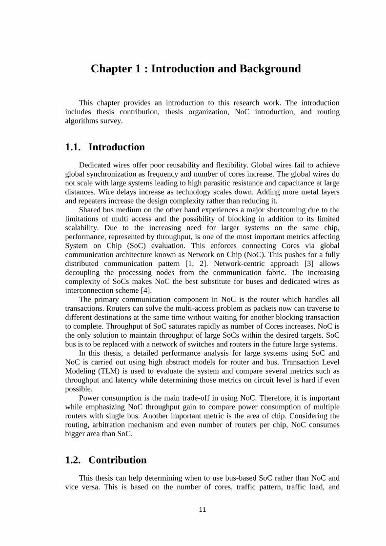
This chapter provides an introduction to this research work. The introduction
includes thesis contribution, thesis organization, NoC introduction, and routing
algorithms survey.
1.1. Introduction
Dedicated wires offer poor reusability and flexibility. Global wires fail to achieve
global synchronization as frequency and number of cores increase. The global wires do
not scale with large systems leading to high parasitic resistance and capacitance at large
distances. Wire delays increase as technology scales down. Adding more metal layers
and repeaters increase the design complexity rather than reducing it.
Shared bus medium on the other hand experiences a major shortcoming due to the
limitations of multi access and the possibility of blocking in addition to its limited
scalability. Due to the increasing need for larger systems on the same chip,
performance, represented by throughput, is one of the most important metrics affecting
System on Chip (SoC) evaluation. This enforces connecting Cores via global
communication architecture known as Network on Chip (NoC). This pushes for a fully
distributed communication pattern [1, 2]. Network-centric approach [3] allows
decoupling the processing nodes from the communication fabric. The increasing
complexity of SoCs makes NoC the best substitute for buses and dedicated wires as
interconnection scheme [4].
The primary communication component in NoC is the router which handles all
transactions. Routers can solve the multi-access problem as packets now can traverse to
different destinations at the same time without waiting for another blocking transaction
to complete. Throughput of SoC saturates rapidly as number of Cores increases. NoC is
the only solution to maintain throughput of large SoCs within the desired targets. SoC
bus is to be replaced with a network of switches and routers in the future large systems.
In this thesis, a detailed performance analysis for large systems using SoC and
NoC is carried out using high abstract models for router and bus. Transaction Level
Modeling (TLM) is used to evaluate the system and compare several metrics such as
throughput and latency while determining those metrics on circuit level is hard if even
possible.
Power consumption is the main trade-off in using NoC. Therefore, it is important
while emphasizing NoC throughput gain to compare power consumption of multiple
routers with single bus. Another important metric is the area of chip. Considering the
routing, arbitration mechanism and even number of routers per chip, NoC consumes
bigger area than SoC.
1.2. Contribution
This thesis can help determining when to use bus-based SoC rather than NoC and
vice versa. This is based on the number of cores, traffic pattern, traffic load, and
11
frequency. Different comparisons are made for performance metrics such as
throughput, latency, number of hops traversed by each packet in addition to power
consumption. These comparisons are made for different traffic loads and with different
number of cores. Building a TLM for router and comparing it with another bus model
helps offering better evaluation based on transactions rather than pin level data.
1.3. Organization of the thesis
A brief summary on NoC architectures, switching techniques and components are
provided in chapter 1. The routing algorithms are considered as the router model is the
basic unit in this work. An introduction to transaction level modeling which is used
throughout this thesis is presented. Both router and bus models and how time and
power are modeled are presented in Chapter 2. Chapter 3 includes literature survey on
traffic generation and also performance evaluation of NoCs. Simulation results and
comparison between NoC and SoC models are described in Chapter 4. The chapter also
includes summary of the results. Finally Chapter 5 includes conclusion and Chapter 6
includes future work. Appendix A includes the router model code. Appendix B includes
the CPU model code. Appendix C includes the traffic generation code.
1.4. NoC Introduction
This section includes a brief introduction to NoC architectures, flow control,
switching techniques, router components, and NoC topologies.
1.4.1. Interconnect Network Architectures
Shared-medium bus is a simple interconnect architecture where all cores share the
same communication medium and bandwidth [4]. These networks support broadcast
and multicast which is an advantage in case the information is needed to be sent to
many receivers [2]. Arbitration is needed if different masters need to access the bus. A
disadvantage of shared bus is its limited scalability.
Direct networks overcome the scalability problem where each node is connected to
set of neighboring nodes [2]. The problem here is long global wires spanning around
the design.
Indirect networks are switch-based ones where nodes are connected through a set
of switches. They solve both the scalability and long wires problems [2]. Hybrid
networks also exist which include heterogeneous connections between bus and
switches.
1.4.2. Flow Control Units
Memories and processing elements are connected to routers through network
interfaces that manage connection and data fragmentation functions [3, 5]. Flow control
deals with allocation of channel and buffer resources to packets as they traverse paths
through the network. For packet-switched networks, the packet is the smallest unit that
contains routing and sequencing information. Each packet is divided into data units
called flits and buffers are defined as multiples of the flit-data unit. A flit is the smallest
unit on which flow control is performed. Information flows on a physical channel as
11
physical transfer units called phits where a phit is the same size of a flit or smaller [6].
Input and output buffers of routers should store few flits only which decreases buffer
space requirements in NoC routers [3].
1.4.3. Switching Techniques
Switching techniques determine when and how internal switches connect inputs to
outputs. Different switching techniques include [2, 3]:
a- Circuit Switching: The transmission first sets a physical path from source to
destination. This end-to-end reserved path causes unnecessary delay. This is
used to guarantee throughput connections [4].
b- Packet Switching: The message is divided into fixed-size packets that are
routed individually without resource reservation. This is advantageous for short
and frequent packets leading to better utilization.
c- Wormhole Switching: first flit is the header flit containing routing information
that enables switch establishing path to destination. Subsequent flits flow in a
pipelined fashion without need of any packet reordering. If any flit faces a busy
channel, all subsequent flits wait. The path is released when the tail packet is
received. Virtual channels increase channel utilization as flits can use other
virtual channels if one of them is blocked. This is used in best effort
connections [4].
1.4.4. Router Architecture
The architecture of NoC router consists of several components [3]:
a- Crossbar: The components connecting input buffers to output ones.
b- Network Interface: Responsible for segmentation of packets and re-ordering
them. Other related work in [7] introduces low power network interface for
NoC.
c- Routing and Arbitration: Routing defines the path for each packet from
source to destination while arbitration selects one input port from different
requests.
d- Buffers: FIFO units storing flits, it is considered the dominant factor in area
cost function for the router. Other work including [8-10] studies area
optimization for buffers.
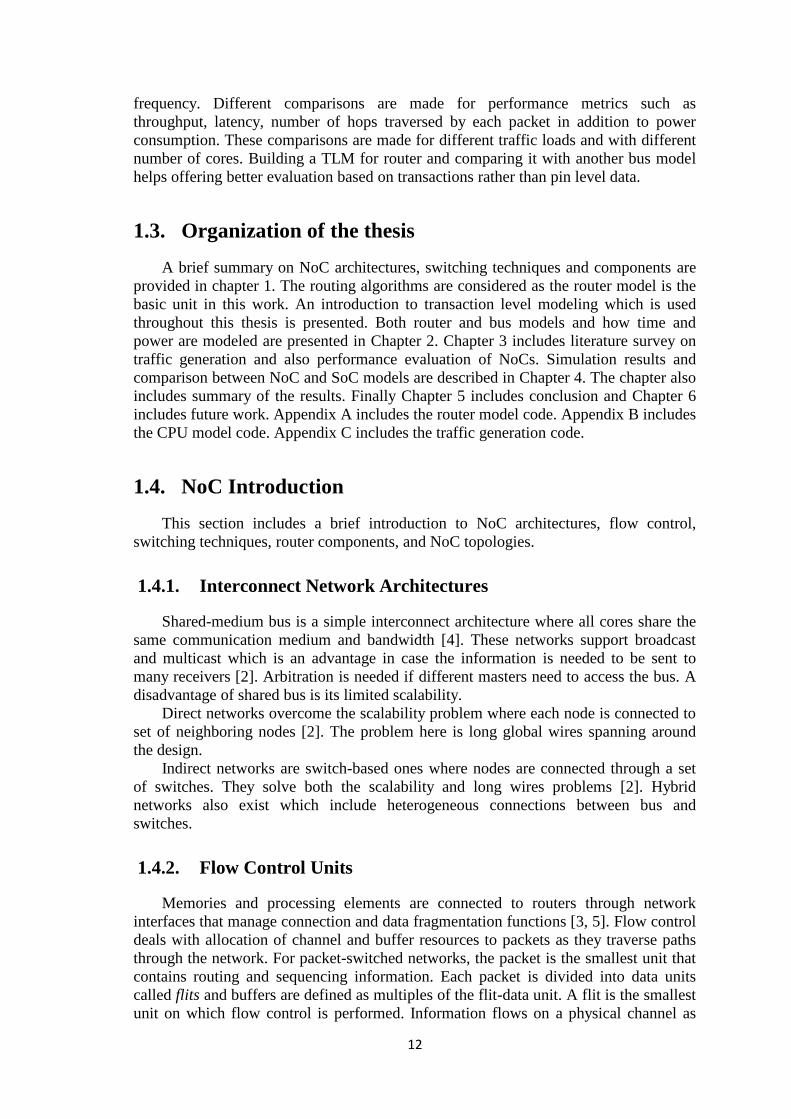
A state diagram of router operation example is shown in Figure 1.1 where S0: type
determination, S1: Routing, S2: Output virtual channel allocation, S3: router allocation,
S4: physical channel allocation, S5: router traversal.

11
Figure 1.1: Router state diagram
1.4.5. NoC Topologies
The topology specifies how the routers and cores are connected to each other.
Commonly used topologies are mentioned below [5] [11-13]:
a- 2D Mesh: The 2D mesh topology is illustrated in Figure 1.2 (a) [5] and Figure
1.3 (a) [13] where each router has 5 ports (north, east, south, west, and local)
and connected to its four neighbors except for border routers. The router
address is easily defined by its x-y coordinates.
b- Ring: Low performance ring topology with low complexity is shown in Figure
1.2 (b).
c- Spidergon: The spidergon connection is shown in Figure 1.2 (c) where each
router has three connections, one for left neighbor, right neighbor, and central
connection. The benefit of this topology is that packets consume only two hops
for any path.
d- Torus: Just like mesh topology but connecting routers at the edge with routers
at the opposite edge via wrap-around channels. Folded torus doubles the
bandwidth by wrapping leftmost routers to rightmost ones and from top
component to bottom. Torus and folded torus are shown in Figure 1.3 (b) and
Figure 1.3 (c) respectively.
e- Fat Tree: Both Fat Tree and Butterfly Fat Tree (BFT) topologies are illustrated
in Figure 1.3 (d) and Figure 1.3 (e) respectively. Fat tree implementation puts
routers and nodes while cores are located at leaves. Each node has four children
and a parent. This is replicated four times at any level of the tree.

11
f- BFT: In Butterfly Fat Tree, each switch has six ports, four for child ports and
two for parents. The intermediate nodes act as switches, four cores are
connected to the children ports at the first level of switches. In the second level,
parents are connected to two switches. The tree architecture has two benefits,
component-level decomposition and congestion reduction.
Figure 1.2: (a) 2D Mesh, (b) Ring, (c) Spidergon, (d) Crossbar
Figure 1.3: NoC architectures
The next sections include different routing algorithms and arbitration algorithms.
1.5. Routing Algorithms
Routing determines the path of each packet traversing the network till reaching its
destination. Routing can be classified according to different criteria into the following
classifications [11, 12]:
1.5.1. Source and Distributed Routing
In distributed routing, the routing decision is taken at each router. The router does
not need global knowledge about network status as it computes the next hop according
to the destination address of each packet [14].
Source routing stores routing tables which contain routing information for each
packet. The header packet must be transmitted throughout the whole network as it
contains the information for each hop in its path to destination. Source routing is not
11
considered in NoCs due to its large overhead to store entire path information in the
header. Also it does not provide adaptive paths in case of congestion or link failure as
the path is pre-computed. However, source routing has its own advantages especially in
NoC with fixed size and regular topology like mesh. Also, it can fit irregular networks
since it is topology independent.
With efficient coding, the router design is significantly simplified. Also for
application specific networks, the traffic profile can help determining paths for desired
performance metrics. Still large size of routing tables results in performance overhead.
1.5.2. Deterministic and Adaptive Routing
Deterministic routing specifies a fixed output link for each destination at each hop.
Thus, the routing information is determined statically and this leads to constant number
of hops for each source-destination pair and may lead to congestion if many packets
have the same destination. Deterministic routing is not dead-lock free due to reasons
mentioned above; also routing fails if any link is broken.
Adaptive routing makes the decision dynamic according to different specifications
such as network load, deadlock, and broken links. For each source-destination pair,
there are several paths leading to different number of hops each time a packet is
transferred from the same source to the same destination.
Centralized adaptive routing monitors global traffic load instead of local
congestion signals, it modifies routing of packets in order to improve load balancing
and outperform distributed adaptive routing [15]. Adaptive routing can be based on
power model which adapts routing according to power conditions in order to optimize
power distribution leading to a power-aware adaptive routing scheme [16].
1.5.3. Routing Algorithms Examples
This section includes examples for the commonly used routing algorithms.
a- XY Routing
XY routing algorithm is a kind of deterministic distributed algorithm. Each router
is identified by its coordinates Cx and Cy (2-dimension mesh topology) [17]. The
algorithm compares router coordinates to destination coordinates Dx and Dy. When
(Cx, Cy) match (Dx, Dy), the packet is transferred to local router port which means that
packet reaches its destination core. Otherwise, horizontal addresses are compared first
till the flit is horizontally aligned. Then the vertical address is compared till reaching
the required destination.
As XY algorithm is deterministic, if any port is busy the packet is blocked as there
is no other routes to the destination so it cannot avoid deadlock. XY algorithm is
illustrated below:
Algorithm XY
/*Source router: (Sx,Sy);destination router: (Dx,Dy); current
router: (Cx,Cy).*/
begin
if (Dx>Cx) //eastbound messages
return E;
else
11
if (Dx<Cx) //westbound messages
return W;
else
if (Dx=Cx) { //currently in the same column as
//destination
if (Dy<Cy) //southbound messages
return S;
else
if (Dy>Cy) //northbound messages
return N;
else
if (Dy=Cy) //current router is the destination router
return C;
}
End
b- OE Routing
Odd-even routing algorithm is a distributed adaptive algorithm based on odd-even
turn model that avoids deadlock through some restrictions [17]. In this model, a column
is called even if its horizontal dimension is an even numerical value and called odd if
its horizontal dimension is an odd number. Since E, S, W, N indicate East, South, West,
and North respectively, there are eight types of turns where a turn is a 90-degree change
of travelling direction. ES turn involves change of direction from East to South.
Similarly, there are EN, WS, WN, SE, SW, NE, and NW turns.
Two main theorems define the OE algorithm:
Theorem 1: NO packet is permitted to do EN turn in each node which is located on
an even column. Also, No packet is permitted to do NW turn in each node that is
located on an odd column.
Theorem 2: NO packet is permitted to do ES turn in each node that is in an even
column. Also, no packet is permitted to do SW turn in each node which is in an odd
column. Where the OE algorithm is presented as:
Algorithm OE
/*Source router: (Sx,Sy);destination router: (Dx,Dy); current
router: (Cx,Cy).*/
begin
avail_dimension_set<-empty;
Ex<-Dx-Cx;
Ey<-Dy-Cy;
if (Ex=0 && Ey=0) //current router is destination
return C;
if (Ex=0){ //current router in same column as //destination
if (Ey<0)
add S to avail_dimension_set;
else
add N to avail_dimension_set;
}
else{
if (Ex>0){ //eastbound messages
if (Ey=0){ //current in same row as destination
11
add E to avail_demision_set;
}
else{
if(Cx % 2 != 0 or Cx=Sx) //N/S turn allowed only in odd
//column.
if(Ey < 0)
add S to avail_dimension_set;
else
add N to avail_dimension_set;
if(Dx% 2 != 0 or Ex != 1) {
//allow to go E only if destination
// is odd column
add E to avail_dimension_set;
//because N/S turn not allowed in
//even column
}
}
}
else { // westbound messages
add W to avail_dimension_set;
if(Cx%2=0) //allow to go N/S only in even
//column, because N->W and S->W
//not allowed in odd column
if(Ey<0)
add S to avail_dimension_set;
else
add N to avail_dimension_set;
}
}
Select a dimension from avail_dimension_set to forward the packet.
end
Providing a group of routing paths for each source-destination pair can prevent
deadlock without using virtual channels.
c- Segment-Based Routing
Link failures lead to irregular topologies and these need routing algorithms that
adapt to static and dynamic changes in irregular topologies [18]. Reconfiguration at the
routing level allows topology changes that can be used in case of switch or link failure.
Segment-based Routing (SR) methodology allows computation of different deadlock-
free routing algorithms by different segmentation processes and routing restriction
policies.
The straightforward routing algorithm used in irregular networks is Up*/Down*
(UD) which selects a root node and performs breadth-first search (BFS) to build a
spanning tree. The algorithm assigns links directions and turn restrictions where the
packet can reach destination by traversing the tree upwards and then downwards.
Therefore, cyclic dependency can be avoided by forbidding up link after a down one.
This algorithm accumulates traffic near root node and the UD tree is fixed as long as
the root node is selected.
11
The SR algorithm uses divide-and-conquer approach by partitioning the topology
to subnets and segments. SR places bidirectional turn restrictions locally to each
segment leading to much more flexibility compared with UD. The final step in SR is
computing final path for each source-destination pair.
SR is a partly adaptive routing algorithm which can be applied on networks that
support deterministic or adaptive routing and on routers that support routing tables. SR
is agnostic to the topology of the network as it is based on network segmentation and
guaranteeing full connectivity between end nodes. However, many patterns for
segments exist and each pattern can affect performance according to topology and
traffic pattern.
Unitary segments contain only one link. Any dependency using these segments
should be forbidden in order to ensure deadlock-freedom. Smart selection during
segmentation can limit unitary segments.
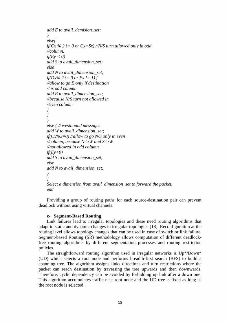
d- Region-Based Routing
Region-based routing (RBR) groups destinations into network regions in order to
reduce number of entries in routing tables. RBR is a general mechanism that can be
used along with any adaptive routing algorithm. RBR mainly targets reducing high area
and power consumption of table-based routers especially in large networks by dividing
network regions and allowing efficient implementation using logic blocks. RBR exhibit
low and constant memory and area requirements regardless of network size [19].
Figure 1.4: Example of region definition
2-D mesh topology networks has the property that the number of required regions
is either constant or grows slowly as network size grows. Also the region computation
is performed offline, downloaded to routers and then network is set into normal
operation. This guarantees no impact on network performance. Regions should take
into consideration restrictions applied by routing algorithm in order not to lead to a
deadlock.
The mechanism in brief starts by receiving network topology and routing
restrictions. Then it computes possible set of routing paths between each pair of nodes.
12
The routing regions can be computed according to routing options at each router.
Finally the algorithm packs all regions in order to bound maximum number of allowed
regions. An example for region computation is shown in Figure 1.4.
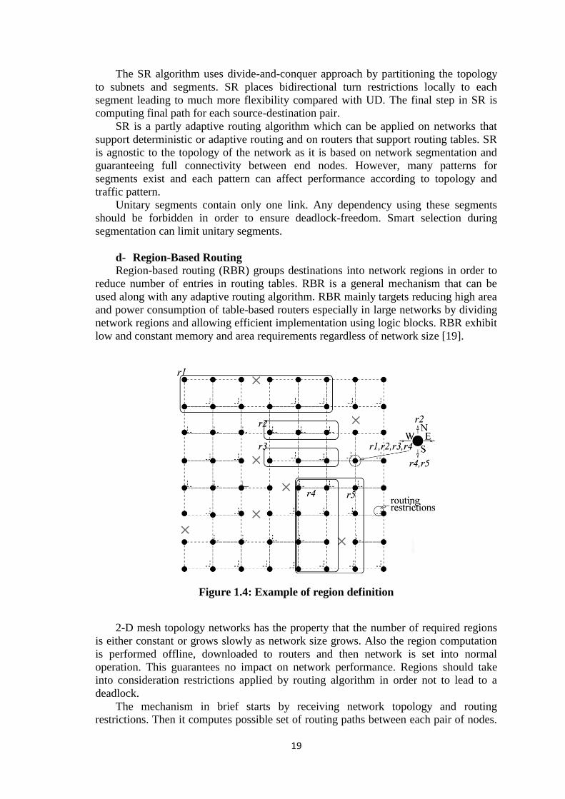
e- Application Specific Routing
Application Specific Routing Algorithm (APSRA) processes the information of
communicating pair of nodes and other pairs that never communicate and also analyze
the concurrency of communication transactions across nodes. This can maximize
communication adaptivity and performance and offer efficient, dead-lock free routing
without the need for virtual channels. APSRA is topology agnostic that best fits NoCs
that are specialized for a set of concurrent/non-concurrent applications. The general
implementation of the routing function is table-based [20]. The ASPRA design
methodology is shown in Figure 1.5.
In the embedded systems domain, the designer has an idea about the set of
applications that is mapped on the system. The routing algorithm does not have to
guarantee that every pair of nodes can communicate. After the task mapping and
scheduling, the designer has information about pairs of communicating nodes as well as
concurrent/non-concurrent transactions.
Figure 1.5: ASPRA Design Methodology
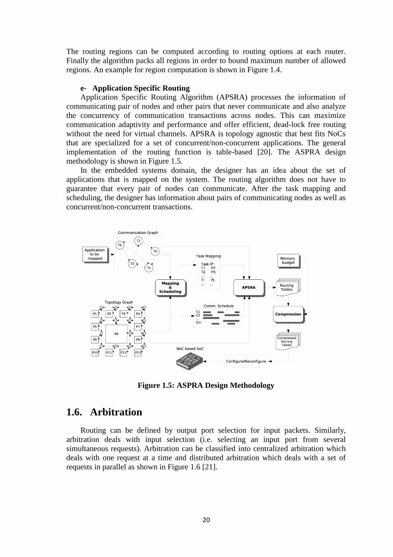
1.6. Arbitration
Routing can be defined by output port selection for input packets. Similarly,
arbitration deals with input selection (i.e. selecting an input port from several
simultaneous requests). Arbitration can be classified into centralized arbitration which
deals with one request at a time and distributed arbitration which deals with a set of
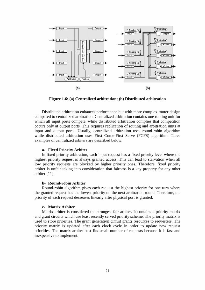
requests in parallel as shown in Figure 1.6 [21].
11
Figure 1.6: (a) Centralized arbitration; (b) Distributed arbitration
Distributed arbitration enhances performance but with more complex router design
compared to centralized arbitration. Centralized arbitration contains one routing unit for
which all input ports compete, while distributed arbitration complies that competition
occurs only at output ports. This requires replication of routing and arbitration units at
input and output ports. Usually, centralized arbitration uses round-robin algorithm
while distributed arbitration uses First Come-First Serve (FCFS) algorithm. Three
examples of centralized arbiters are described below.
a- Fixed Priority Arbiter
In fixed priority arbitration, each input request has a fixed priority level where the
highest priority request is always granted access. This can lead to starvation when all
low priority requests are blocked by higher priority ones. Therefore, fixed priority
arbiter is unfair taking into consideration that fairness is a key property for any other
arbiter [11].
b- Round-robin Arbiter
Round-robin algorithm gives each request the highest priority for one turn where
the granted request has the lowest priority on the next arbitration round. Therefore, the
priority of each request decreases linearly after physical port is granted.
c- Matrix Arbiter
Matrix arbiter is considered the strongest fair arbiter. It contains a priority matrix
and grant circuits which use least recently served priority scheme. The priority matrix is
used to store priorities. The grant generation circuit grants resources to requesters. The
priority matrix is updated after each clock cycle in order to update new request
priorities. The matrix arbiter best fits small number of requests because it is fast and
inexpensive to implement.
11
1.7. Related Work
This section includes a literature survey on related work to compare between NoCs
and shared buses medium. This thesis refers to buses with SoCs while NoCs are using
routers.
1.7.1. NoC Comparison
Erno Salminen et al. [22] presented state-of-the-art paper in the field of NoC
benchmarking and comparison. The paper gathered and analyzed a vast set of studies
from literatures. The following basic NoC properties are considered:
1- Offering scalability.
2- Avoiding global wires spanning the chip.
3- Supporting system testing.
The paper summarizes network comparisons found in literature and analyzes them
according to:
1- Compared Topologies.
2- Evaluation Type.
3- Evaluation Criteria.
The runtime and latency are the most popular metric in the studied literature. In
general, achieving the same latency with less area and power is the evaluation criteria.
The results from literature seem confusing as every study use tests with different
characteristics and requirements and performance always depend on application.
Finally, the paper proposes practical basic guidelines for simulation and benchmarking.
These guidelines are divided into:
1- Workload.
2- System Model.
3- Measurement.
4- Concluding the Findings.
The paper does not provide quantified results for throughput comparison. This thesis
includes quantitative performance evaluation for NoC and SoC.
1.7.2. Multi-synchronous vs. Asynchronous
Sheibanyard et al. [1] presented a systematic comparison between fully
asynchronous and multi-synchronous NoC architectures that are used in Globally
Asynchronous Locally Synchronous (GALS) multi processors system on chip. The five
relevant parameters which are used in the comparison are:
Silicon area.
Network saturation threshold.
Throughput.
Latency.
Power consumption.
The first implementation is Distributed Scalable Predictable Interconnect Network
(DSPIN) and the second implementation is Asynchronous Scalable Predictable
Interconnect Network (ASPIN). Multi synchronous systems contain one or several
synchronous subsystems clocked with independent clocks and connected with micro
network as illustrated in Figure 1.7 [1].

11
Figure 1.7: Multi-synchronous system
Partitioning the SoC into isolated clusters allows timing closure independently for
each cluster without any time constraints. This can solve the long wire issue in multi-
million gate SoCs. The research uses a long wire model and extracted SPICE model for
DSPIN and ASPIN components in order to evaluate latency, throughput, and power
consumption.
For power consumption, the work focuses on instantaneous energy consumption
during one short period of time using current integrator model. The asynchronous
approach shows better saturation thresholds and better latency but with higher energy
dissipation. The comparison does not include SoC to compare with which is considered
in this thesis.
1.7.3. QoS Communication Schemes
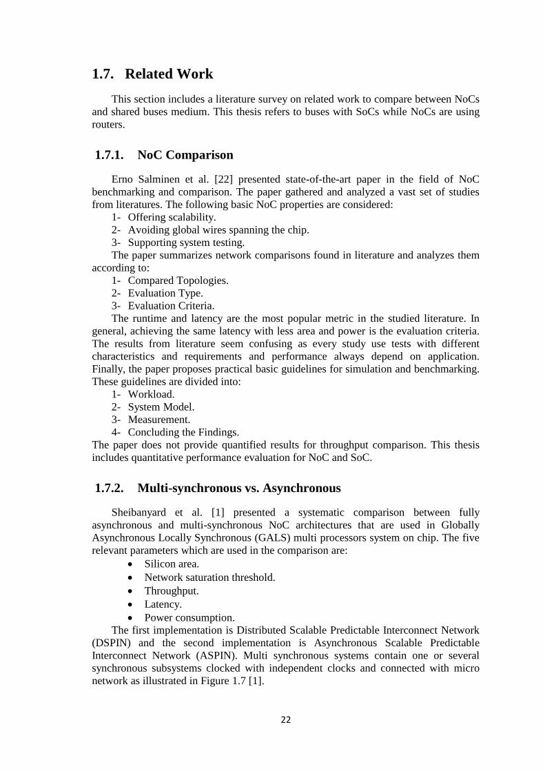
Mehmet Derin Harmanci et al. [23] addressed quantitative comparison of
connection-oriented and connectionless-oriented communication schemes. These
communication schemes are used to guarantee Quality of Service (QoS). QoS is
defined by several parameters such as availability, jitter, packet loss, and throughput.
For QoS, it is necessary to have global predictability about the NoC. Virtual channel is
an example of building connection-oriented communication on top of packet switched
network where independent input channels are multiplexed over the same physical link.
The main disadvantage of this scheme is in-efficient resources reservation and non-
scalability.
Connectionless-oriented scheme can be applied by implementing additional
services to meet predefined QoS parameters like prioritization of flows. This offers a
better adaptation to the varying network traffic and better utilization of network
resources. A SystemC model is built for both communication schemes as shown in
Figure 1.8 [23]. The simulation considers only end-to-end delay by using nodes that run
MPEG-2 algorithms along with random noise. This thesis considers performance
metrics such as throughput, latency, number of hops, and power consumption.
11
Figure 1.8: (a) Connection-oriented router (b) Connectionless-oriented router
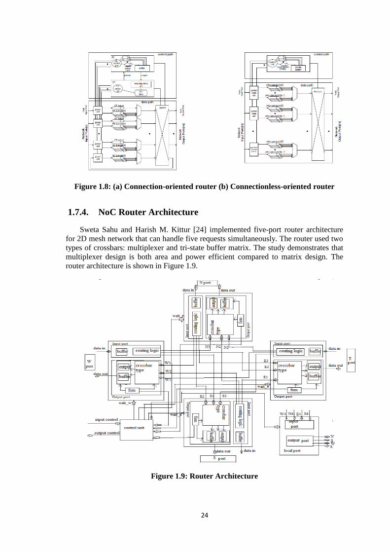
1.7.4. NoC Router Architecture
Sweta Sahu and Harish M. Kittur [24] implemented five-port router architecture
for 2D mesh network that can handle five requests simultaneously. The router used two
types of crossbars: multiplexer and tri-state buffer matrix. The study demonstrates that
multiplexer design is both area and power efficient compared to matrix design. The
router architecture is shown in Figure 1.9.
Figure 1.9: Router Architecture
11
This work uses wormhole switching, XY deterministic routing algorithm, and
simple round-robin arbiters. The five ports of the router allow dynamic placement of
modules in NoC mesh network. Each port has its own decoding logic to increase the
router performance. The power and area are analyzed and compared for 90nm and
180nm technologies. Other performance metrics such as throughput and latency are not
evaluated which is considered in this thesis.
1.7.5. Comparison of Æthereal NoC and Bus
Chris Bartels et al. [25] applied Æthereal NoC to bus based SoC and performed
area comparison between the two architectures down to netlist level. Æthereal NoC
offers Guaranteed Throughput (GT) aided with predictability and decoupling of the
behavior of one core from other cores and interconnects. Therefore, the performance of
core is not affected by the others. This work uses digital video terrestrial receiver
design (DVB-T) and compares the original bus-based SoC with different NoC-based
solutions.
The main interconnect structure of the SoC is ARM AMBA High-speed Bus AHB
which is replaced with NoC in order to perform the comparison. The NoC shows 60%
area savings but with higher buffer cost. The comparison does not include throughput
and latency metrics.
The Best Effort (BE) service class guarantees reception of data without minimum
bandwidth or maximum latency bounds. GT service class use Time Division Multiple
Access (TDMA) to give worst-case guarantees on bandwidth and latency. Both GT and
BE use source routing where the path to destination is determined at the source router.
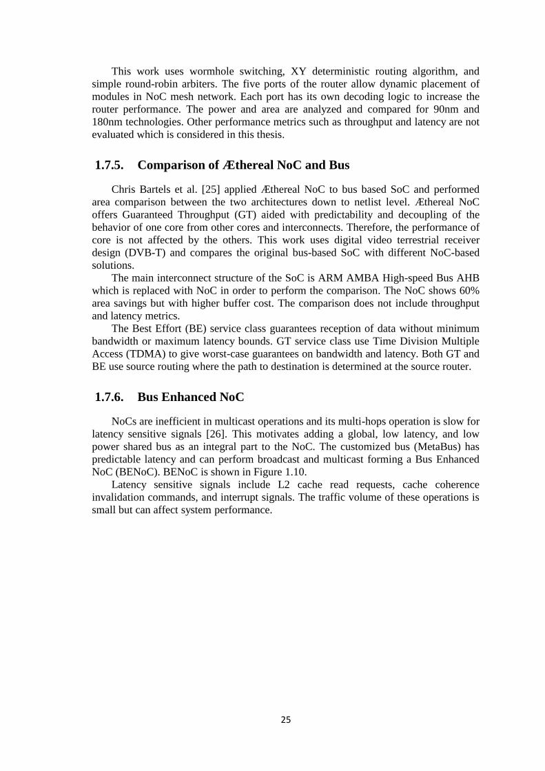
1.7.6. Bus Enhanced NoC
NoCs are inefficient in multicast operations and its multi-hops operation is slow for
latency sensitive signals [26]. This motivates adding a global, low latency, and low
power shared bus as an integral part to the NoC. The customized bus (MetaBus) has
predictable latency and can perform broadcast and multicast forming a Bus Enhanced
NoC (BENoC). BENoC is shown in Figure 1.10.
Latency sensitive signals include L2 cache read requests, cache coherence
invalidation commands, and interrupt signals. The traffic volume of these operations is
small but can affect system performance.
11
Figure 1.10: BENoC
BENoC’s bus sends messages that are different than those delivered by the
network such as control and multicast messages. This study compares area and latency
of BENoC and that of pure NoC. The study showed that BENoC is more advantageous
than classic NoC and the advantage increases as system size grows. The comparison
does not include throughput or power metrics which are included in this thesis.
1.7.7. Bus and NoC Comparison
Ling Wang et al. [27] studied and compared the performance of Bus with NoC
Spidernet and mesh topologies implemented in FPGA. Spidernet NoC is shown in
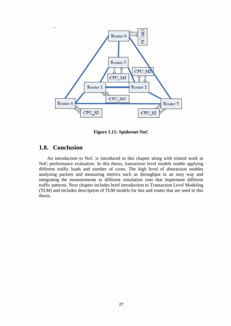
Figure 1.11. The inner triangle of Spidernet topology forms the basic structure in the
network and then spread to three directions to form the outer one. The masters are
distributed within the inner triangle while slaves are distributed in the outer triangle.
The work in this paper uses latency and area as evaluation metrics of the bus and
NoC performance. It uses two types of emulation flow where the emulation system is
implemented in Altera FPGA. This paper does not include other evaluation metrics
such as throughput and power consumption.
The results show that Spidernet offers better latency than that of Mesh-based NoC
and that of shared bus. Throughput comparison is not illustrated in this paper. Other
related work is found in [28] [33] [35-37]. Also [4] introduced state of the art in routers
that use virtual channels.
11
Figure 1.11: Spidernet NoC
1.8. Conclusion
An introduction to NoC is introduced in this chapter along with related work in
NoC performance evaluation. In this thesis, transaction level models enable applying
different traffic loads and number of cores. The high level of abstraction enables
analyzing packets and measuring metrics such as throughput in an easy way and
integrating the measurements in different simulation runs that implement different
traffic patterns. Next chapter includes brief introduction to Transaction Level Modeling
(TLM) and includes description of TLM models for bus and router that are used in this
thesis.

11
Chapter 2 : Router and Bus Models
2.1. Introduction
The basics of the modeling technique which is used in this thesis are introduced in
this chapter. A brief introduction to TLM is presented and then detailed description for
bus and router models which are used in SoC and NoC, respectively, is discussed.
2.1.1. Modeling Levels
Modeling accuracy can vary from very detailed implementation model to cycle-
accurate RTL model to more abstract model which increases simulation speed, protect
more detailed intellectual property, and inject stimuli and check results quickly [29].
The several independent axes that can control model accuracy include structural
accuracy, functional accuracy, and timing accuracy. Other axes may include data
organization accuracy and communication protocol accuracy. Different time models
can be classified into:
Untimed Functional Model:
Direct translation of design specification without any time delays in the model.
Communications between modules are point-to-point without any shared
communication links.
Timed Functional Model:
The module’s communication is still point-to-point but the model includes time
delays that describe timing constraints of the specification and delay of particular target
implementation.
Transaction-Level Model (TLM):
Communications between modules are modeled by function calls that are
implemented with functional and timing accuracy (sometimes even accurate to the
clock-cycle level). Still the model is not structurally accurate.
Behavioral Hardware Model:
Pin-accurate and functionally accurate but does not have internal structure that
reflects target implementation. Usually these models are input to behavioral hardware
synthesis tools.
Register Transfer Level (RTL) Model:
Pin-accurate and cycle-accurate model with internal structure that reflects
accurately registers and combinational logic of target implementation.
This thesis focuses on transaction-level modeling which is a discrete-event model
of computation where function calls represent transactions. Each transaction has a start
time, end time and payload data. System synchronization scheme is needed in order to
ensure predictable and deterministic system execution. This is implemented in this
11
thesis by means of interrupts. TLM designs are generally more concise and have shorter
simulation time than corresponding RTL designs.
2.1.2. Transaction Level Modeling
Abstraction is a powerful technique for design and implementation of complex
systems where unnecessary details can be hidden. TLM is a high-level approach to
modeling systems. Buses and FIFOs are modeled as channels and presented using
SystemC interface classes. Transactions take place by function calls to these interface
classes. Transactions encapsulate low-level details of information exchange. Thus,
TLM focus more on functionality rather than implementation. This approach is easier
for system-level design [29].
Synchronization details in TLM are abstracted into blocking and non-blocking I/O
where priorities are assigned to bus masters and centralized arbitration is modeled.
TLM is used for timed and untimed functional modeling, platform modeling, and
testbench construction. Taking bus modeling as an example, aspects such as contention,
arbitration, interrupts, and cycle-accuracy can be modeled away from pin-accurate
models. In general, TLMs are important as they are easy to develop and understand.
TLM can be constructed at an early stage in system design process, and they are
quickly simulated.
SystemC “sc_fifo” is an example of untimed functional TLM for First In First Out
(FIFO) channel, where the transaction interfaces are represented through the read and
write methods of this channel. "sc_fifo” models the FIFO functionality typically but
with much simpler implementation than actual hardware. TLM is not limited to buses
and FIFOs as the same principles can be applied to any high-order communication
mechanism.
The TLM model needs to be cycle-accurate so that it can serve as an agreed-upon
contract between software and hardware teams. This feature along with high simulation
speed can allow meaningful amount of software code to be executed along with
hardware model.
For any model, the transaction interfaces are the starting point to understand how
the design operates [30]. The interfaces are shown in Figure 2.1 and can be classified
into:
Blocking Interfaces:
In blocking interface, the communication methods return only after transaction
completion. Typically for bus models where there is no multi-access, the masters use
blocking transactions.
Non-blocking Interfaces:
In non-blocking interface, the methods return immediately while the transaction
takes at least one clock cycle to complete. The transaction may take more than one
clock cycle if competing requests exist. This interface is commonly used by processor
models which cannot be suspended.

12
Figure 2.1: Blocking and non-blocking interfaces [30]
Direct Interfaces:
These operations are used to create a simulation monitor for the design and for
debugging purposes. During these methods, SystemC scheduler does not intervene and
simulation time does not advance. This interface should not be used as part of design
implementation, but can be used as a part of the testbench for the design.
2.1.3. Modeling for High Performance
TLM uses some techniques for high performance simulation, as the model is not
pin-accurate, the data within transaction can be bundled and passed more efficiently.
Thus TLM relies on transaction rather than signals. Also high-level data types are used
rather than low-level bit-vectors which are commonly used in HDLs [29]. Pointers to
data are passed between modules through transactions which enable copying blocks of
data efficiently.
SystemC dynamic sensitivity feature is used to eliminate unnecessary activation of
processes. RTL models must execute every clock edge even without any activity. This
results in performance gain for TLM compared to RTL.
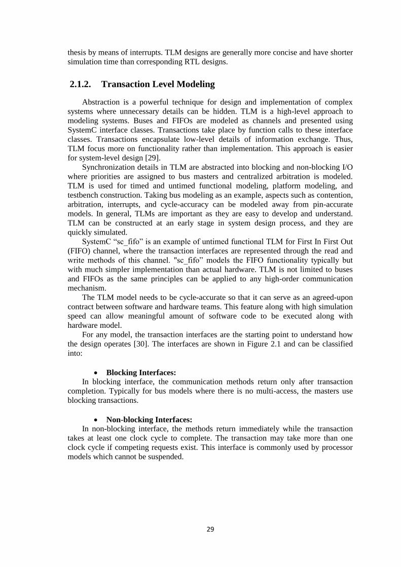
2.1.4. The Scalable Model Approach
The scalable TLM model is a property of Mentor Graphics’ Vista tool which is
based on separation of functionality, communication, and architecture. The untimed
functionality is captured in programmable view (PV) layer while timing and power are
defined in the “T” layer. “PV” and “T” are combined in a single “PVT” model [30].
The PVT model is shown in Figure 2.2.
11
Figure 2.2: PVT model structure [30]
Architectural impacts such as communication protocols, different burst sizes, and
input-to-output latencies are captured in the “T” model without changing the “PV” one.
This can allow software validation and virtual prototyping by just shutting down the
“T” layer in order to run pure functional simulation.
The behavior of the model is described by how it reacts to incoming transactions.
This behavior is defined in salve port’s callback function; these reactive functions
implement model’s functionality. Similar callback functions are defined for registers as
it is a common modeling practice to program a model using a set of control registers.
The register can trigger the callback function upon accessing the register.
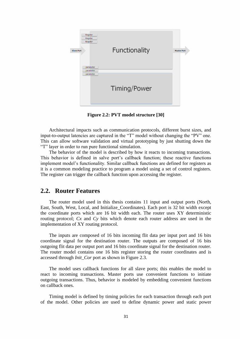
2.2. Router Features
The router model used in this thesis contains 11 input and output ports (North,
East, South, West, Local, and Initialize_Coordinates). Each port is 32 bit width except
the coordinate ports which are 16 bit width each. The router uses XY deterministic
routing protocol; Cx and Cy bits which denote each router address are used in the
implementation of XY routing protocol.
The inputs are composed of 16 bits incoming flit data per input port and 16 bits
coordinate signal for the destination router. The outputs are composed of 16 bits
outgoing flit data per output port and 16 bits coordinate signal for the destination router.
The router model contains one 16 bits register storing the router coordinates and is
accessed through Init_Cor port as shown in Figure 2.3.
The model uses callback functions for all slave ports; this enables the model to
react to incoming transactions. Master ports use convenient functions to initiate
outgoing transactions. Thus, behavior is modeled by embedding convenient functions
on callback ones.
Timing model is defined by timing policies for each transaction through each port
of the model. Other policies are used to define dynamic power and static power
11
consumption as well as clock tree power dissipation. Routing mechanism is
implemented through C++ defined functions that parse coordinates bits for each
transaction, and determine the next hop and outgoing port through XY routing
algorithm.
Figure 2.3: Router model
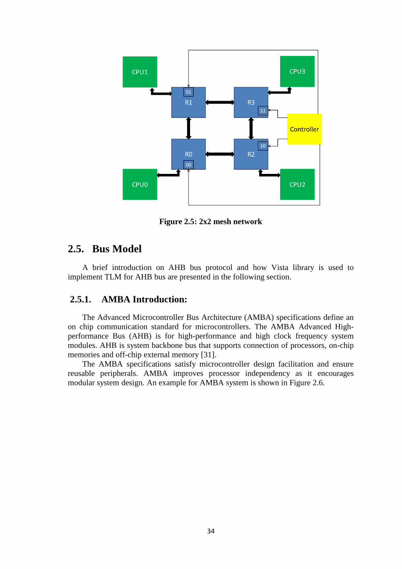
A special CPU is used to initialize the coordinates of each router according to its
location in the mesh network. After coordinates initialization, an interrupt request is
sent to each core in order to start sending and receiving data packets. An example of the
mesh network is illustrated in Figure 2.5.
2.3. Modeling Timing for the Router:
Timing in TLM is modeled by policies like Delay, Pipeline, and Split that use
internal latencies and buffering. Transactions are executed using function calls and such
abstraction increases simulation speed. Internal FIFOs and buffers break packets into
smaller groups that are processed in parallel, these macro architectures are explored
through timing policies. Timing policies are modeled using non-blocking transactions
where each transaction is composed of several phases and each of which is executed
with its own timing attributes.
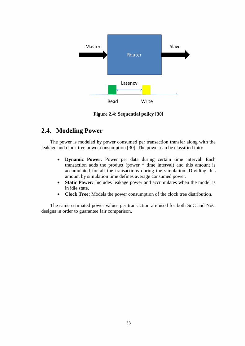
The router model uses the “Sequential Policy” to model timing attributes of
transmitted packets. A latency is defined for master transactions and input/output
trigger (the Cause) while different latencies can be defined to different triggers. The
sequential policy is shown in Figure 2.4.
11
Figure 2.4: Sequential policy [30]
2.4. Modeling Power
The power is modeled by power consumed per transaction transfer along with the
leakage and clock tree power consumption [30]. The power can be classified into:
Dynamic Power: Power per data during certain time interval. Each
transaction adds the product (power * time interval) and this amount is
accumulated for all the transactions during the simulation. Dividing this
amount by simulation time defines average consumed power.
Static Power: Includes leakage power and accumulates when the model is
in idle state.
Clock Tree: Models the power consumption of the clock tree distribution.
The same estimated power values per transaction are used for both SoC and NoC
designs in order to guarantee fair comparison.
11
Figure 2.5: 2x2 mesh network
2.5. Bus Model
A brief introduction on AHB bus protocol and how Vista library is used to
implement TLM for AHB bus are presented in the following section.
2.5.1. AMBA Introduction:
The Advanced Microcontroller Bus Architecture (AMBA) specifications define an
on chip communication standard for microcontrollers. The AMBA Advanced High-
performance Bus (AHB) is for high-performance and high clock frequency system
modules. AHB is system backbone bus that supports connection of processors, on-chip
memories and off-chip external memory [31].
The AMBA specifications satisfy microcontroller design facilitation and ensure
reusable peripherals. AMBA improves processor independency as it encourages
modular system design. An example for AMBA system is shown in Figure 2.6.

11
Figure 2.6: Typical AMBA system
2.5.2. AMBA AHB
AMBA AHB implements burst transfers and split transactions that may contain
more than one bus master such as Direct Memory Access (DMA) or Digital Signal
Processor (DSP) [31].
Typical AHB system contains the following components:
AHB Master: Initiates read and write operations.
AHB Slave: Responds to read and write operations.
AHB Arbiter: Ensures that only one master can access the bus at a time.
AHB Decoder: Decodes the address to provide select signal for the
required slave.
The AHB provides a high bandwidth solution. In addition, the single-clock-edge
protocol offers smooth integration in ASIC environment. AHB Lite is a subset of high-
speed bus architecture AHB. AHB Lite allows only one master, requiring no arbitration
and saving some signals (request, grant, split …etc.) Multi-layer AHB (ML-AHB) is an
interconnect architecture that extends the AHB bus architecture that provides parallel
accesses between multiple masters and slaves to increase overall bandwidth and
performance. However, the interconnection matrix has higher cost compared to
standard AHB [25]. An example for n-layer AHB system is shown in Figure 2.7.

11
Figure 2.7: N-layer AHB system [25]
2.5.3. Modeling Timing for AHB Bus
Pipeline timing policy is used to model the bus behavior; the pipeline policy is
implemented by AHB bus in response to any initiated master transaction. Pipeline
policy is illustrated in Figure 2.8.
Figure 2.8: Pipeline policy [30]
2.5.4. Bus Arbitration
The bus model supports priority-based arbitration. A predefined priority parameter
is defined so that different priorities can be specified per master [30] [32] [34]. Round-
robin arbitration is used in this design where all cores have the same priority. Changing
the arbitration scheme directly affects simulation results as low priority masters take
more time to complete their transactions which degrade latency and throughput. An
example for bus model connection is shown in Figure 2.9.

11
Figure 2.9: Bus model [30]
2.6. Conclusion
A brief introduction to TLM is presented in this chapter. Detailed description for
bus and router models is discussed where router model is implemented in NoC and bus
model is implemented in SoC. In the next chapter, a literature survey for traffic
generation is presented along with the traffic generation technique which is used for
simulation in the thesis.

11
Chapter 3 : Traffic Generation
3.1.1. Introduction
This chapter includes a literature survey for related work to traffic generation in
NoC simulation. The traffic generation technique which is used in this thesis is also
discussed. Performance evaluation and design space exploration is very important for
SoC development [38]. Traffic Generation (TG) should provide fast and effective
simulation environment in addition to fast architectural exploration by trying
interconnection alternatives. It has been estimated that NoC performance may vary up
to 250% according to NoC design and up to 600% depending on communication traffic
model [5]. This emphasizes the importance of accurate traffic modeling and generation
for NoC evaluation.
3.2. Traffic Kinds
There are three commonly used types of traffic [39]:
a- Application driven traffic: This models network and IPs simultaneously
based on copying communication traces after real-time simulation.
b- Synthetic traffic: Easier design and manipulation as it captures the salient
aspects only of application driven traffic and that is why it is widely used for
network evaluation.
c- Application oriented traffic: It is between application-driven and synthetic
traffic where time specifications and message size can be either synthetic or
captured from execution traces [40].
3.3. Emulating IP Communication Behavior
The IP emulating traffic generator model captures type and time stamp of
communication events at the IP interface in a reference environment [38]. The TG
captures the resulting reactiveness to access patterns and resource contention. Thus, the
regenerated traffic represents realistic workload which is independent from the
interconnect architecture. This TG model increases the speed of complete NoC
simulation as the architectural exploration involves carrying out the same experiment
with different architectures. Still this TG requires the presence of reference NoC
design. The reference NoC includes either software compiled and executed by IPs or
synthesized code into dedicated hardware. This reference model is used to collect traces
of IP behavior. The IPs are then replaced with TGs emulating the IP communication at
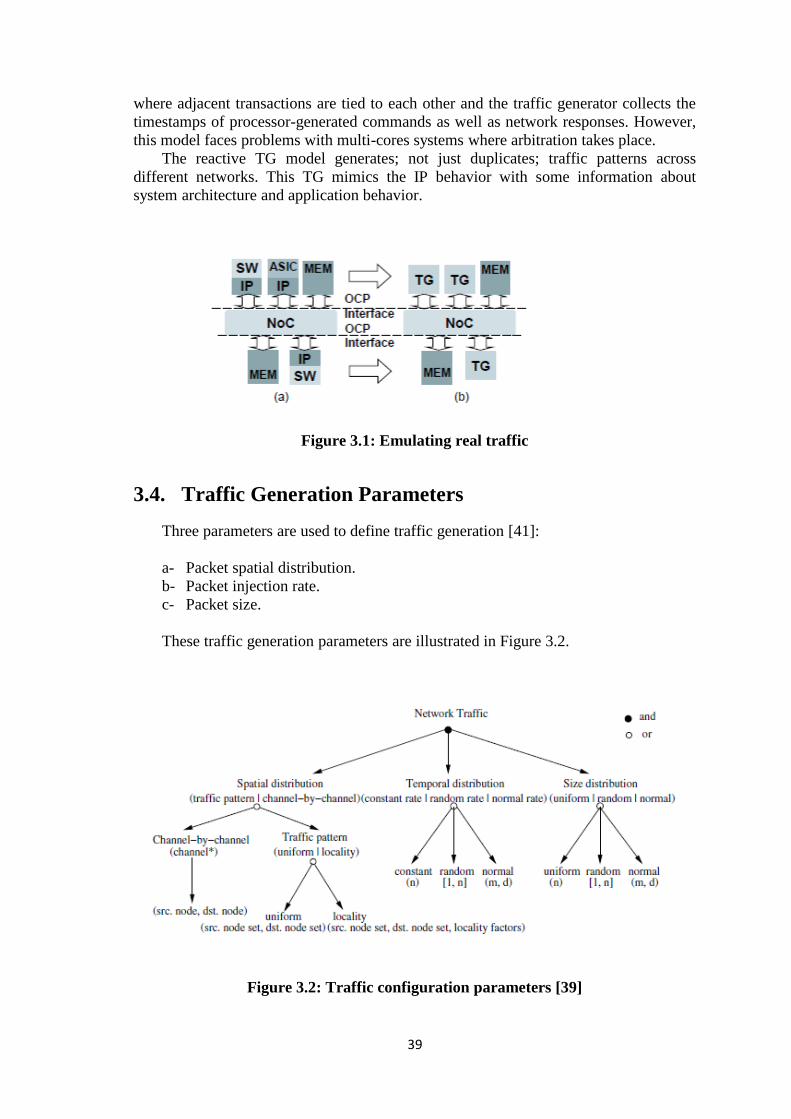
the network interface as shown in Figure 3.1 [38]. Therefore, only one reference
simulation using bit and cycle accuracy is needed, and then subsequent simulations are
carried out by the traffic generator replacements.
At very basic level, collecting traces with timestamps from reference model and
replaying is called “cloning”. This approach fails under consideration of network
latency. When one transaction is delayed, subsequent transaction should be delayed as
well. Thus another approach is used which is called “time-shifting” traffic generator
11
where adjacent transactions are tied to each other and the traffic generator collects the
timestamps of processor-generated commands as well as network responses. However,
this model faces problems with multi-cores systems where arbitration takes place.
The reactive TG model generates; not just duplicates; traffic patterns across
different networks. This TG mimics the IP behavior with some information about
system architecture and application behavior.
Figure 3.1: Emulating real traffic
3.4. Traffic Generation Parameters
Three parameters are used to define traffic generation [41]:
a- Packet spatial distribution.
b- Packet injection rate.
c- Packet size.
These traffic generation parameters are illustrated in Figure 3.2.
Figure 3.2: Traffic configuration parameters [39]

12
Packet spatial distribution specifies the relation between sources and destinations.
It can be classified into traffic pattern and channel-by-channel traffic [39]; with traffic
pattern all channels share the same timing and size parameters while channel-by-
channel traffic specifies different parameters for each channel. In addition, source-
destination pairs are fixed throughout the whole simulation; this can be used to
construct application-oriented workloads [40].
The most widely used patterns are Bit Reversal, Perfect Shuffle, Butterfly, Matrix
Transpose, and Complement. An example for Complement traffic pattern is shown in
Figure 3.3. Most of related work use only random patterns. Non-uniform traffic patterns
are closer to real applications as they cause traffic concentrations and hot spots.
Random patterns can take different distributions such as Normal, Uniform (all
nodes have the same probability to be destinations), Exponential, and Poisson.
Temporal distribution can be Static (Constant), Normal, and Random. The packet
injection rate is a fraction of channel maximum bandwidth in bits per second. This
thesis uses a Random traffic pattern with each source transmitting successive packets
separated by a random number of clock cycles between zero and ten.
Figure 3.3: Complement traffic pattern [41]
3.5. Configurable Traffic Generator
Due to the need for fast and effective generation environment for evaluating NoC
performance, configurable traffic generators became widely used [40]. The traffic
generation parameters which are discussed above are adjusted in order to save
simulation time.
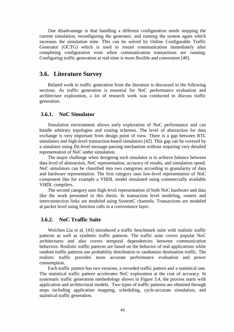
11
One disadvantage is that handling a different configuration needs stopping the
current simulation, reconfiguring the generator, and running the system again which
increases the simulation time. This can be solved by Online Configurable Traffic
Generator (OCTG) which is used to restart communication immediately after
completing configuration even when communication transactions are running.
Configuring traffic generation at real-time is more flexible and convenient [40].
3.6. Literature Survey
Related work to traffic generation from the literature is discussed in the following
sections. As traffic generation is essential for NoC performance evaluation and
architecture exploration, a lot of research work was conducted to discuss traffic
generation.
3.6.1. NoC Simulator
Simulation environment allows early exploration of NoC performance and can
handle arbitrary topologies and routing schemes. The level of abstraction for data
exchange is very important from design point of view. There is a gap between RTL
simulators and high-level transaction-based simulators [42]. This gap can be covered by
a simulator using flit-level message-parsing mechanism without requiring very detailed
representation of NoC under simulation.
The major challenge when designing such simulator is to achieve balance between
data level of abstraction, NoC representation, accuracy of results, and simulation speed.
NoC simulators can be classified into two categories according to granularity of data
and hardware representation. The first category uses low-level representation of NoC
component like for example a VHDL model simulated using commercially available
VHDL compilers.
The second category uses high-level representation of both NoC hardware and data
like the work presented in this thesis. In transaction level modeling, routers and
interconnection links are modeled using SystemC channels. Transactions are modeled
at packet level using function calls in a convenience layer.
3.6.2. NoC Traffic Suite
Weichen Liu et al. [43] introduced a traffic benchmark suite with realistic traffic
patterns as well as synthetic traffic patterns. The traffic suite covers popular NoC
architectures and also covers temporal dependencies between communication
behaviors. Realistic traffic patterns are based on the behavior of real applications while
random traffic patterns use probability distribution to randomize destination traffic. The
realistic traffic provides more accurate performance evaluation and power
consumption.
Each traffic pattern has two versions, a recorded traffic pattern and a statistical one.
The statistical traffic pattern accelerates NoC exploration at the cost of accuracy. In
systematic traffic generation methodology shown in Figure 3.4, the process starts with
application and architectural models. Two types of traffic patterns are obtained through
steps including application mapping, scheduling, cycle-accurate simulation, and
statistical traffic generation.
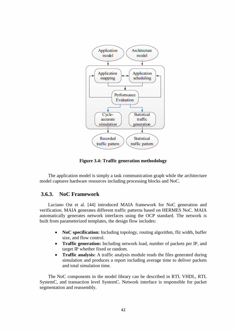
11
Figure 3.4: Traffic generation methodology
The application model is simply a task communication graph while the architecture
model captures hardware resources including processing blocks and NoC.
3.6.3. NoC Framework
Luciano Ost et al. [44] introduced MAIA framework for NoC generation and
verification. MAIA generates different traffic patterns based on HERMES NoC. MAIA
automatically generates network interfaces using the OCP standard. The network is
built from parameterized templates, the design flow includes:
NoC specification: Including topology, routing algorithm, flit width, buffer
size, and flow control.
Traffic generation: Including network load, number of packets per IP, and
target IP whether fixed or random.
Traffic analysis: A traffic analysis module reads the files generated during
simulation and produces a report including average time to deliver packets
and total simulation time.
The NoC components in the model library can be described in RTL VHDL, RTL
SystemC, and transaction level SystemC. Network interface is responsible for packet
segmentation and reassembly.
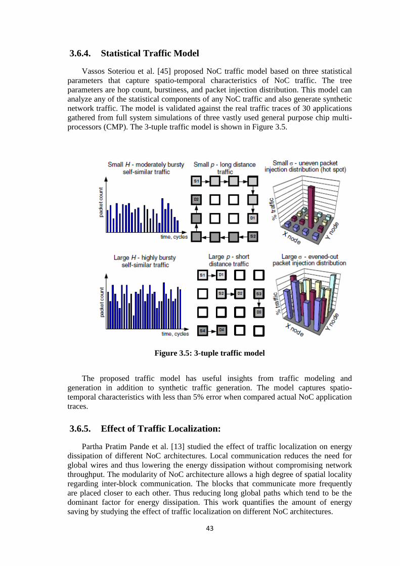
11
3.6.4. Statistical Traffic Model
Vassos Soteriou et al. [45] proposed NoC traffic model based on three statistical
parameters that capture spatio-temporal characteristics of NoC traffic. The tree
parameters are hop count, burstiness, and packet injection distribution. This model can
analyze any of the statistical components of any NoC traffic and also generate synthetic
network traffic. The model is validated against the real traffic traces of 30 applications
gathered from full system simulations of three vastly used general purpose chip multi-
processors (CMP). The 3-tuple traffic model is shown in Figure 3.5.
Figure 3.5: 3-tuple traffic model
The proposed traffic model has useful insights from traffic modeling and
generation in addition to synthetic traffic generation. The model captures spatio-
temporal characteristics with less than 5% error when compared actual NoC application
traces.
3.6.5. Effect of Traffic Localization:
Partha Pratim Pande et al. [13] studied the effect of traffic localization on energy
dissipation of different NoC architectures. Local communication reduces the need for
global wires and thus lowering the energy dissipation without compromising network
throughput. The modularity of NoC architecture allows a high degree of spatial locality
regarding inter-block communication. The blocks that communicate more frequently
are placed closer to each other. Thus reducing long global paths which tend to be the
dominant factor for energy dissipation. This work quantifies the amount of energy
saving by studying the effect of traffic localization on different NoC architectures.
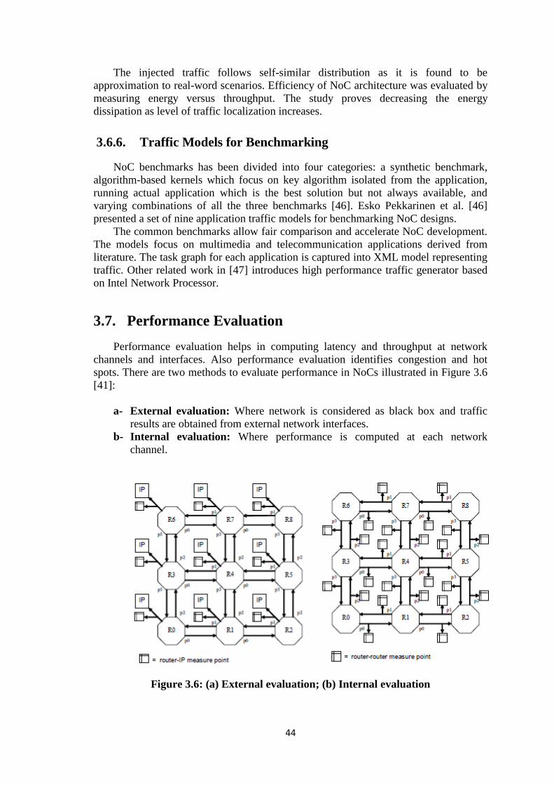
11
The injected traffic follows self-similar distribution as it is found to be
approximation to real-word scenarios. Efficiency of NoC architecture was evaluated by
measuring energy versus throughput. The study proves decreasing the energy
dissipation as level of traffic localization increases.
3.6.6. Traffic Models for Benchmarking
NoC benchmarks has been divided into four categories: a synthetic benchmark,
algorithm-based kernels which focus on key algorithm isolated from the application,
running actual application which is the best solution but not always available, and
varying combinations of all the three benchmarks [46]. Esko Pekkarinen et al. [46]
presented a set of nine application traffic models for benchmarking NoC designs.
The common benchmarks allow fair comparison and accelerate NoC development.
The models focus on multimedia and telecommunication applications derived from
literature. The task graph for each application is captured into XML model representing
traffic. Other related work in [47] introduces high performance traffic generator based
on Intel Network Processor.
3.7. Performance Evaluation
Performance evaluation helps in computing latency and throughput at network
channels and interfaces. Also performance evaluation identifies congestion and hot
spots. There are two methods to evaluate performance in NoCs illustrated in Figure 3.6
[41]:
a- External evaluation: Where network is considered as black box and traffic
results are obtained from external network interfaces.
b- Internal evaluation: Where performance is computed at each network
channel.
Figure 3.6: (a) External evaluation; (b) Internal evaluation

11
Network optimization can be carried out first by identifying hot spots and critical
paths (through traffic generation and performance evaluation). Then structural
optimization can be carried out by inserting virtual channels, eliminate unused links,
and change routing algorithm or network topology. It is preferable for the system to
allow plug-and-play of alternative communication architectures for a given traffic
configuration [48]. This can be made through network interfaces which are architecture
-independent.
3.7.1. Performance Metrics
A standard set of metrics are used to compare and contrast NoC architectures and
evaluate NoC against SoC using shared bus.
a- Throughput: It is the rate of traffic transmitted through the system and can be
defined by [13]:
Throughput =(𝑇𝑜𝑡𝑎𝑙 𝑚𝑒𝑠𝑠𝑎𝑔𝑒𝑠 𝑐𝑜𝑚𝑝𝑙𝑒𝑡𝑒𝑑) × (𝑀𝑒𝑠𝑠𝑎𝑔𝑒 𝑙𝑒𝑛𝑔𝑡ℎ)
(Number of cores) × (𝑇𝑜𝑡𝑎𝑙 𝑡𝑖𝑚𝑒)
As number of cores is the same in case of SoC and NoC, it is omitted from
throughput calculations in this work.
Throughput of the network can also be defined by the data rate per second that the
network can accept [49]. Maximum throughput is achieved when the network reaches
saturation. Accepted traffic can be compared with offered traffic.
b- Latency: It is the time elapsed since packet is injected from source node till the
packet is fully received at destination [50]. Like throughput, the latency
depends on topology and flow control as well as routing algorithm. Zero-load
latency is considered ignoring latency due to contention. Latency can be
compared with offered traffic as well.
c- Power: Power dissipation includes dynamic power, static power, and clock tree
dissipation.
3.8. Conclusion
This chapter includes traffic generation discussion and literature survey for traffic
generation techniques. In the next chapter, simulation for NoC and SoC systems is
discussed. The results of NoC and SoC performance evaluation are illustrated in next
chapter.
11
Chapter 4 : Simulation and Results
4.1. Introduction
Simulation results of NoC and SoC are compared in this chapter. The simulation is
carried out using Mentor Graphics Vista tools. Vista is a native Electronics System
Level (ESL) tool for architecture design, verification analysis, and virtual prototyping
for high-level TLM hardware platforms. Vista uses TLM Scalable Modeling
Methodology relying on C/C++ market standards (gcc) [34]. It also includes TLM2.0
genetic model library that offers fast models for various processors and peripherals
from which AHB model for the bus SoC is used. Vista also offers a model builder with
convenience functions that facilitates building any model by defining ports, timing, and
power policies. And the tool creates SystemC templates based on TLM2.0 socket
initiators and targets.
The model builder offers models built on two completely separate layers:
Programmer View (PV) with pure functional behavior layer.
Timing (T) layer that captures power and timing information through some
timing policies in a top-down flow.
These separate models allow distinction between functionality and implementation.
They allow pure functional simulation (PV) or comprehensive timing and power
behavior simulation (PVT). Finally the tool offers schematic builder for system
assembly, SystemC debugger, and analysis tool used for measuring different metrics
such as throughput, latency, and power.
4.2. NoC Simulation
The same NoC router model is used throughout all simulations (2x2, 3x3, and
4x4). The system design of 2x2 network is shown in Figure 4.1:
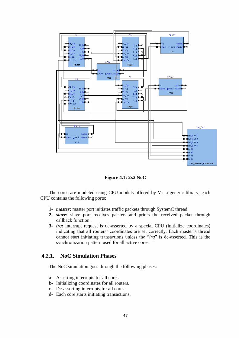
11
Figure 4.1: 2x2 NoC
The cores are modeled using CPU models offered by Vista generic library; each
CPU contains the following ports:
1- master: master port initiates traffic packets through SystemC thread.
2- slave: slave port receives packets and prints the received packet through
callback function.
3- irq: interrupt request is de-asserted by a special CPU (initialize coordinates)
indicating that all routers’ coordinates are set correctly. Each master’s thread
cannot start initiating transactions unless the “irq” is de-asserted. This is the
synchronization pattern used for all active cores.
4.2.1. NoC Simulation Phases
The NoC simulation goes through the following phases:
a- Asserting interrupts for all cores.
b- Initializing coordinates for all routers.
c- De-asserting interrupts for all cores.
d- Each core starts initiating transactions.
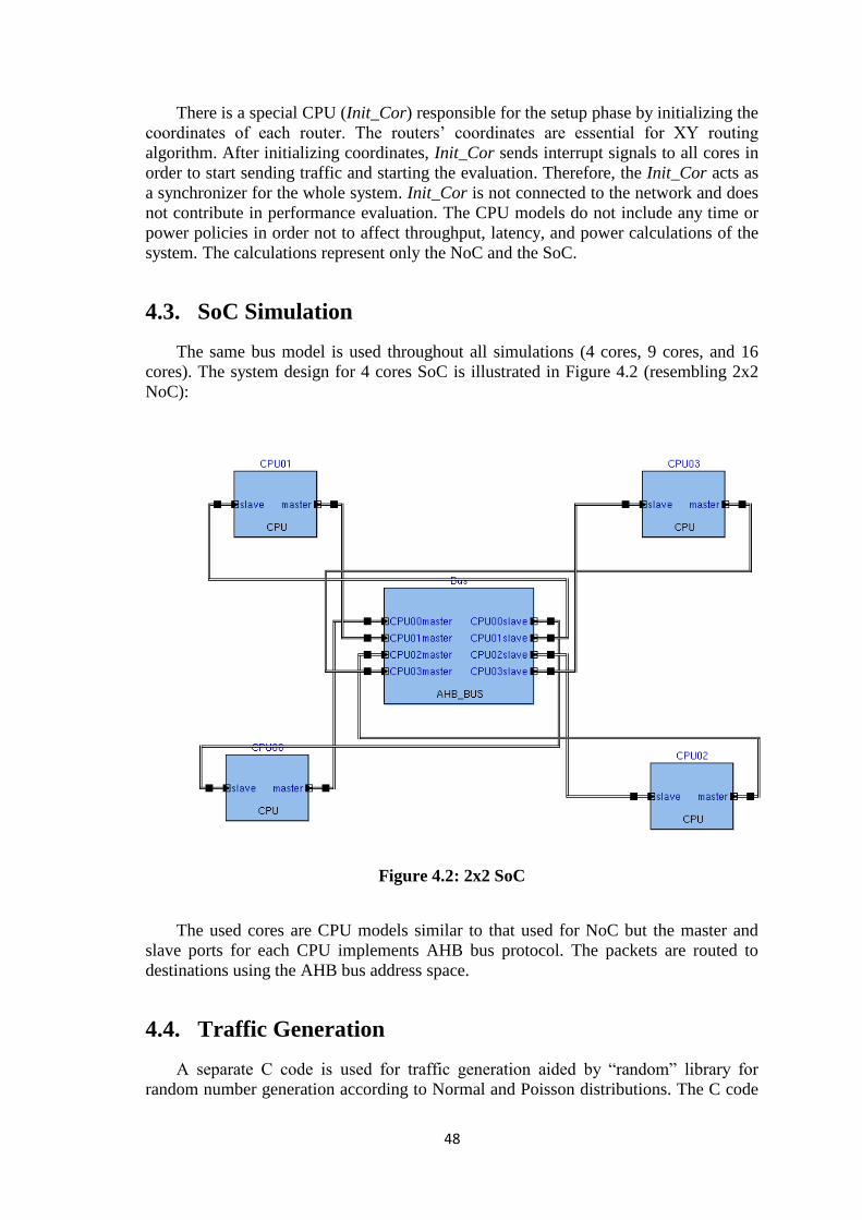
11
There is a special CPU (Init_Cor) responsible for the setup phase by initializing the
coordinates of each router. The routers’ coordinates are essential for XY routing
algorithm. After initializing coordinates, Init_Cor sends interrupt signals to all cores in
order to start sending traffic and starting the evaluation. Therefore, the Init_Cor acts as
a synchronizer for the whole system. Init_Cor is not connected to the network and does
not contribute in performance evaluation. The CPU models do not include any time or
power policies in order not to affect throughput, latency, and power calculations of the
system. The calculations represent only the NoC and the SoC.
4.3. SoC Simulation
The same bus model is used throughout all simulations (4 cores, 9 cores, and 16
cores). The system design for 4 cores SoC is illustrated in Figure 4.2 (resembling 2x2
NoC):
Figure 4.2: 2x2 SoC
The used cores are CPU models similar to that used for NoC but the master and
slave ports for each CPU implements AHB bus protocol. The packets are routed to
destinations using the AHB bus address space.
4.4. Traffic Generation
A separate C code is used for traffic generation aided by “random” library for
random number generation according to Normal and Poisson distributions. The C code
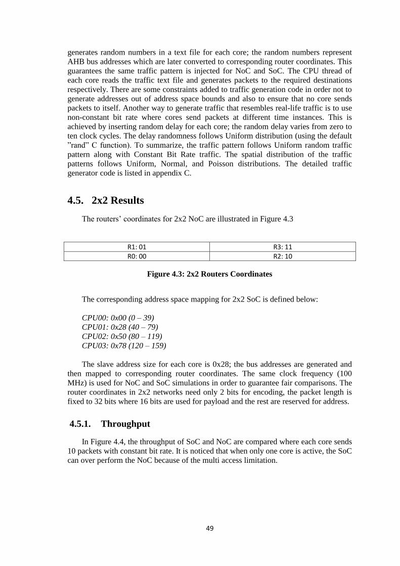
11
generates random numbers in a text file for each core; the random numbers represent
AHB bus addresses which are later converted to corresponding router coordinates. This
guarantees the same traffic pattern is injected for NoC and SoC. The CPU thread of
each core reads the traffic text file and generates packets to the required destinations
respectively. There are some constraints added to traffic generation code in order not to
generate addresses out of address space bounds and also to ensure that no core sends
packets to itself. Another way to generate traffic that resembles real-life traffic is to use
non-constant bit rate where cores send packets at different time instances. This is
achieved by inserting random delay for each core; the random delay varies from zero to
ten clock cycles. The delay randomness follows Uniform distribution (using the default
”rand” C function). To summarize, the traffic pattern follows Uniform random traffic
pattern along with Constant Bit Rate traffic. The spatial distribution of the traffic
patterns follows Uniform, Normal, and Poisson distributions. The detailed traffic
generator code is listed in appendix C.
4.5. 2x2 Results
The routers’ coordinates for 2x2 NoC are illustrated in Figure 4.3
R1: 01 R3: 11
R0: 00 R2: 10
Figure 4.3: 2x2 Routers Coordinates
The corresponding address space mapping for 2x2 SoC is defined below:
CPU00: 0x00 (0 – 39)
CPU01: 0x28 (40 – 79)
CPU02: 0x50 (80 – 119)
CPU03: 0x78 (120 – 159)
The slave address size for each core is 0x28; the bus addresses are generated and
then mapped to corresponding router coordinates. The same clock frequency (100
MHz) is used for NoC and SoC simulations in order to guarantee fair comparisons. The
router coordinates in 2x2 networks need only 2 bits for encoding, the packet length is
fixed to 32 bits where 16 bits are used for payload and the rest are reserved for address.
4.5.1. Throughput
In Figure 4.4, the throughput of SoC and NoC are compared where each core sends
10 packets with constant bit rate. It is noticed that when only one core is active, the SoC
can over perform the NoC because of the multi access limitation.

12
Figure 4.4: Throughput for different active cores
When more than one core is active, the bus arbitrates between different packets and
some packets wait. The router can route packets targeting different addresses at the
same time. The throughput drop between two and three active cores is due to traffic
localization, where the traffic pattern in this experiment is uniformly distributed but
with constraints that CPU02 sends packets to CPU03 and CPU04 and CPU03 sends
packets to CPU04 only. This leads to a hot spot at CPU04 when three cores are active.
The normalized throughput for another experiment is shown in Figure 4.5 where all
cores are active and inject different traffic loads; the same traffic pattern is used with
constant bit rate after modifying the localization constraints. It is noticed that the
throughput slope for the NoC is increasing while the curve for SoC tends to saturate.
The traffic loads vary from 10 packets/core to 320 packets/core as shown on the x-axis.
The throughput percentage change is illustrated in Figure 4.6.

11
Figure 4.5: Normalized throughput for different traffic loads
Figure 4.6: Throughput percentage change (Constant Bit Rate)
Changing the traffic pattern to non-constant bit rate, and using Normal distribution
for spatial traffic pattern, the throughput curve for NoC still has an increasing slope
while the SoC throughput curve tends to saturate at high traffic loads as shown in
Figure 4.7. Throughput percentage change is illustrated in Figure 4.8.
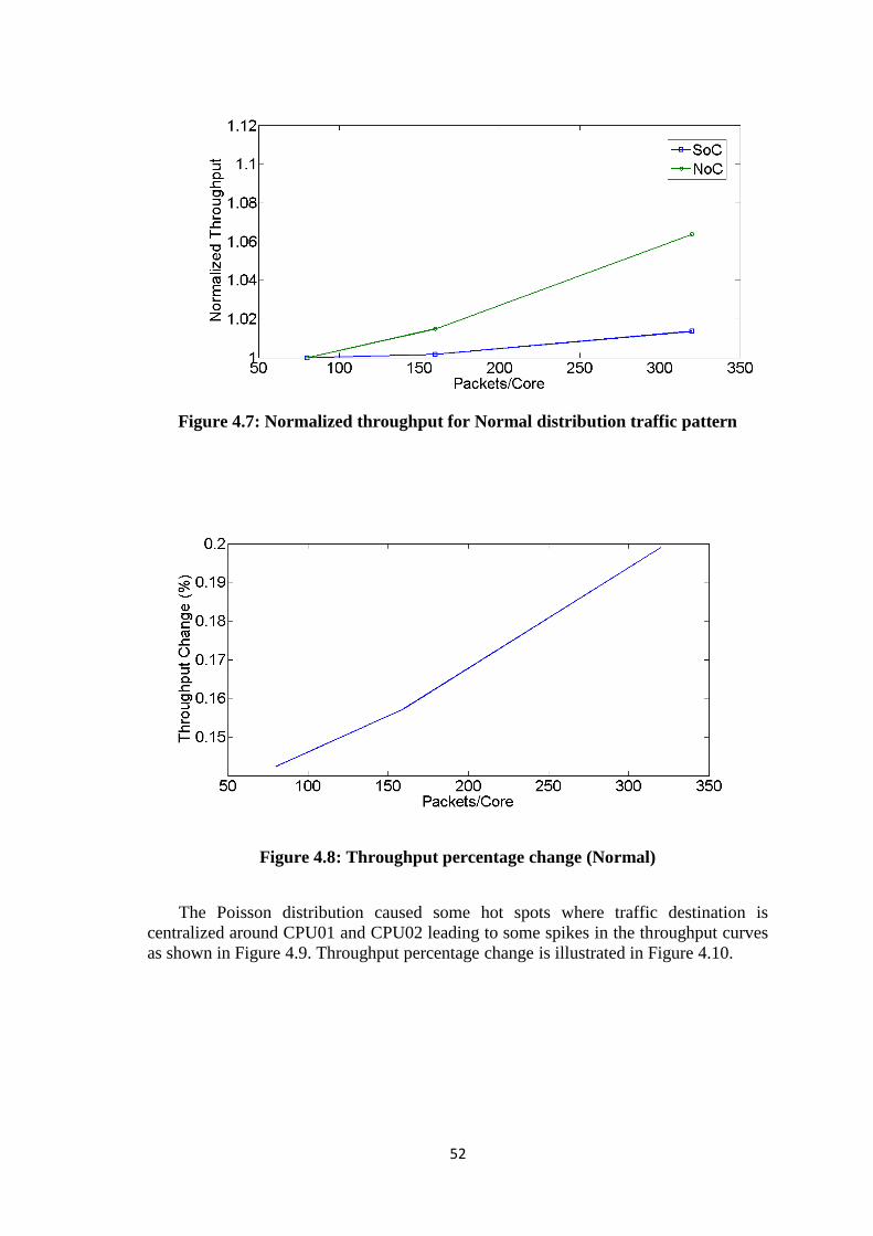
11
Figure 4.7: Normalized throughput for Normal distribution traffic pattern
Figure 4.8: Throughput percentage change (Normal)
The Poisson distribution caused some hot spots where traffic destination is
centralized around CPU01 and CPU02 leading to some spikes in the throughput curves
as shown in Figure 4.9. Throughput percentage change is illustrated in Figure 4.10.
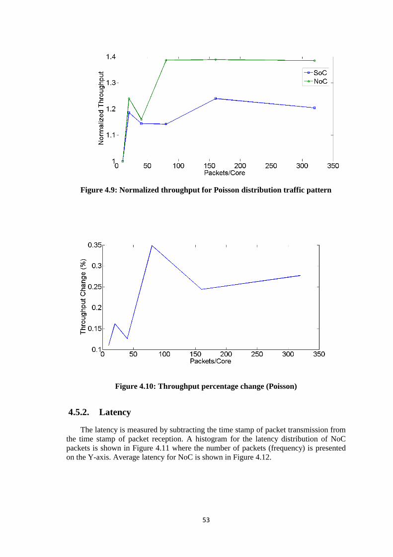
11
Figure 4.9: Normalized throughput for Poisson distribution traffic pattern
Figure 4.10: Throughput percentage change (Poisson)
4.5.2. Latency
The latency is measured by subtracting the time stamp of packet transmission from
the time stamp of packet reception. A histogram for the latency distribution of NoC
packets is shown in Figure 4.11 where the number of packets (frequency) is presented
on the Y-axis. Average latency for NoC is shown in Figure 4.12.
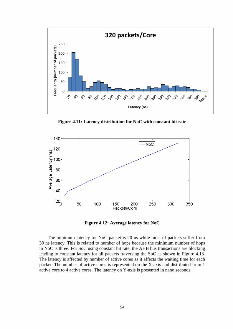
11
Figure 4.11: Latency distribution for NoC with constant bit rate
Figure 4.12: Average latency for NoC
The minimum latency for NoC packet is 20 ns while most of packets suffer from
30 ns latency. This is related to number of hops because the minimum number of hops
in NoC is three. For SoC using constant bit rate, the AHB bus transactions are blocking
leading to constant latency for all packets traversing the SoC as shown in Figure 4.13.
The latency is affected by number of active cores as it affects the waiting time for each
packet. The number of active cores is represented on the X-axis and distributed from 1
active core to 4 active cores. The latency on Y-axis is presented in nano seconds.
0
50
100
150
200
250
Fre
qu
en
cy (
nu
mb
er
of
pac
kets
)
Latency (ns)
320 packets/Core

11
Figure 4.13: SoC Latency
The SoC cores do not transmit packets at the same time when non-constant bit rate
is used. This leads to variable latencies for SoC as well as NoC. It is shown in Figure
4.14, Figure 4.15, Figure 4.16, and Figure 4.17 that for different traffic distributions,
most of NoC packets suffer from 20 ns latency while most of SoC packets suffer from
10 ns latency. This demonstrates that latency sensitive packets are not suitable for NoC
due to higher number of hops. Average latencies for NoC and SoC with different traffic
patterns are illustrated in Figure 4.18, Figure 4.19, Figure 4.20, and Figure 4.21.
Figure 4.14: SoC latency distribution (Normal)
0
100
200
300
400
500
600
700
800
10 20 30 40 50 60 70 More
Fre
qu
en
cy (
nu
mb
er
of
pac
kets
)
Latency (ns)
320 Packets/Core
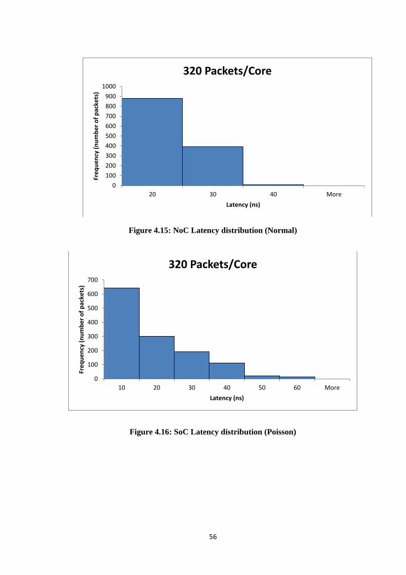
11
Figure 4.15: NoC Latency distribution (Normal)
Figure 4.16: SoC Latency distribution (Poisson)
0
100
200
300
400
500
600
700
800
900
1000
20 30 40 More
Fre
qu
en
cy (
nu
mb
er
of
pac
kets
)
Latency (ns)
320 Packets/Core
0
100
200
300
400
500
600
700
10 20 30 40 50 60 More
Fre
qu
en
cy (
nu
mb
er
of
pac
kets
)
Latency (ns)
320 Packets/Core
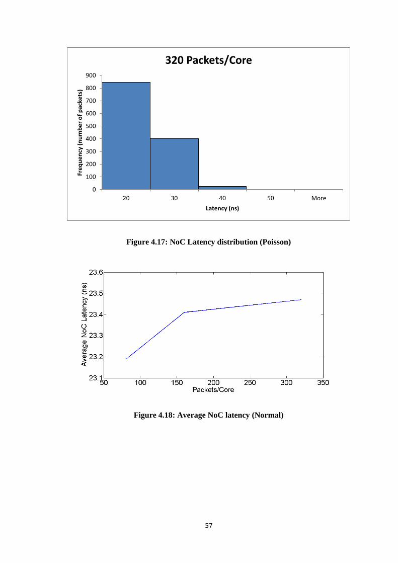
11
Figure 4.17: NoC Latency distribution (Poisson)
Figure 4.18: Average NoC latency (Normal)
0
100
200
300
400
500
600
700
800
900
20 30 40 50 More
Fre
qu
en
cy (
nu
mb
er
of
pac
kets
)
Latency (ns)
320 Packets/Core
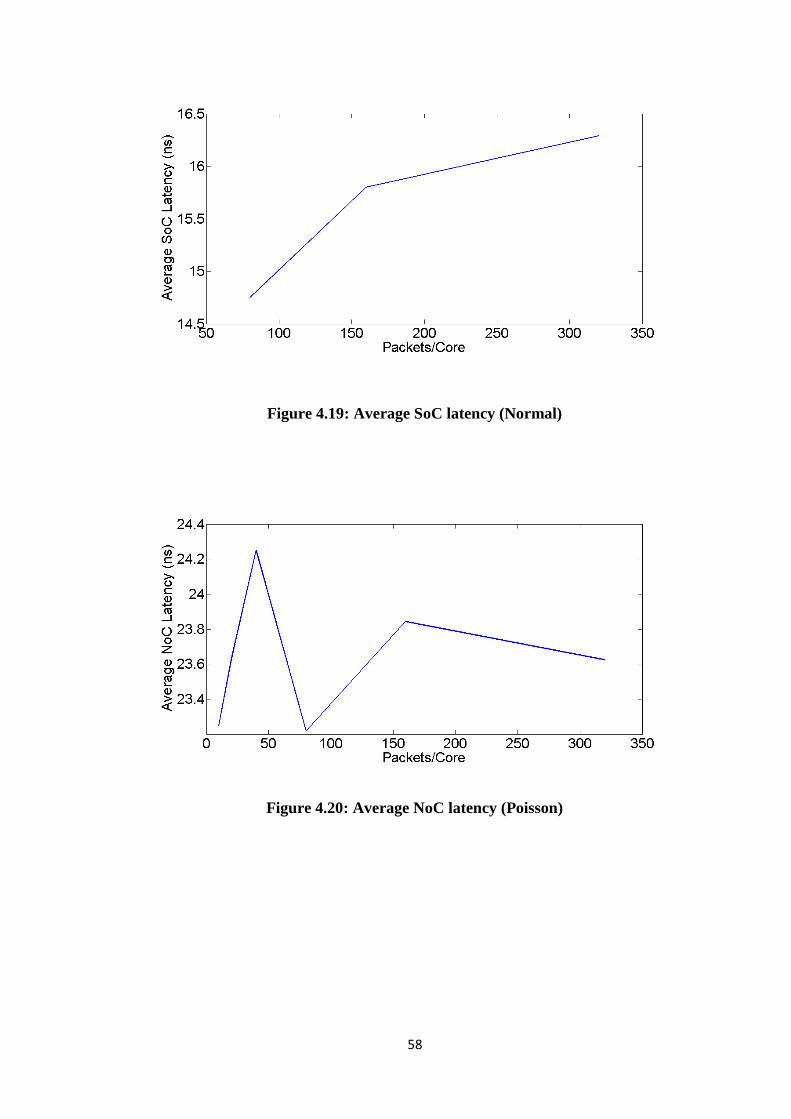
11
Figure 4.19: Average SoC latency (Normal)
Figure 4.20: Average NoC latency (Poisson)
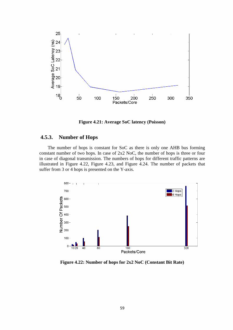
11
Figure 4.21: Average SoC latency (Poisson)
4.5.3. Number of Hops
The number of hops is constant for SoC as there is only one AHB bus forming
constant number of two hops. In case of 2x2 NoC, the number of hops is three or four
in case of diagonal transmission. The numbers of hops for different traffic patterns are
illustrated in Figure 4.22, Figure 4.23, and Figure 4.24. The number of packets that
suffer from 3 or 4 hops is presented on the Y-axis.
Figure 4.22: Number of hops for 2x2 NoC (Constant Bit Rate)

12
Figure 4.23: Number of hops for 2x2 NoC (Normal)
Figure 4.24: Number of hops for 2x2 NoC (Poisson)
4.5.4. Power
Vista classifies power calculations into the following categories:
Dynamic Power: A power number is specified for each timing policy. That
power is consumed from the time the word is transmitted during the latency
parameter time length of the policy.
Static Power: A number is specified representing leakage power in mW.
Clock Tree Distribution: Note that all models used in this work are
synchronous.
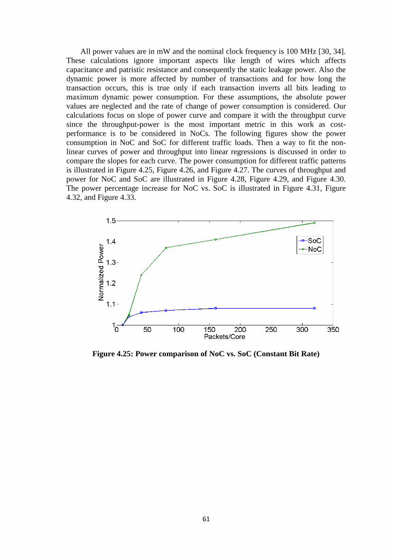
11
All power values are in mW and the nominal clock frequency is 100 MHz [30, 34].
These calculations ignore important aspects like length of wires which affects
capacitance and patristic resistance and consequently the static leakage power. Also the
dynamic power is more affected by number of transactions and for how long the
transaction occurs, this is true only if each transaction inverts all bits leading to
maximum dynamic power consumption. For these assumptions, the absolute power
values are neglected and the rate of change of power consumption is considered. Our
calculations focus on slope of power curve and compare it with the throughput curve
since the throughput-power is the most important metric in this work as cost-
performance is to be considered in NoCs. The following figures show the power
consumption in NoC and SoC for different traffic loads. Then a way to fit the non-
linear curves of power and throughput into linear regressions is discussed in order to
compare the slopes for each curve. The power consumption for different traffic patterns
is illustrated in Figure 4.25, Figure 4.26, and Figure 4.27. The curves of throughput and
power for NoC and SoC are illustrated in Figure 4.28, Figure 4.29, and Figure 4.30.
The power percentage increase for NoC vs. SoC is illustrated in Figure 4.31, Figure
4.32, and Figure 4.33.
Figure 4.25: Power comparison of NoC vs. SoC (Constant Bit Rate)

11
Figure 4.26: Power comparison of NoC vs. SoC (Normal)
Figure 4.27: Power comparison of NoC vs. SoC (Poisson)

11
Figure 4.28: Normalized Throughput and Power (Constant Bit Rate)
Figure 4.29: Normalized Throughput and Power (Normal)
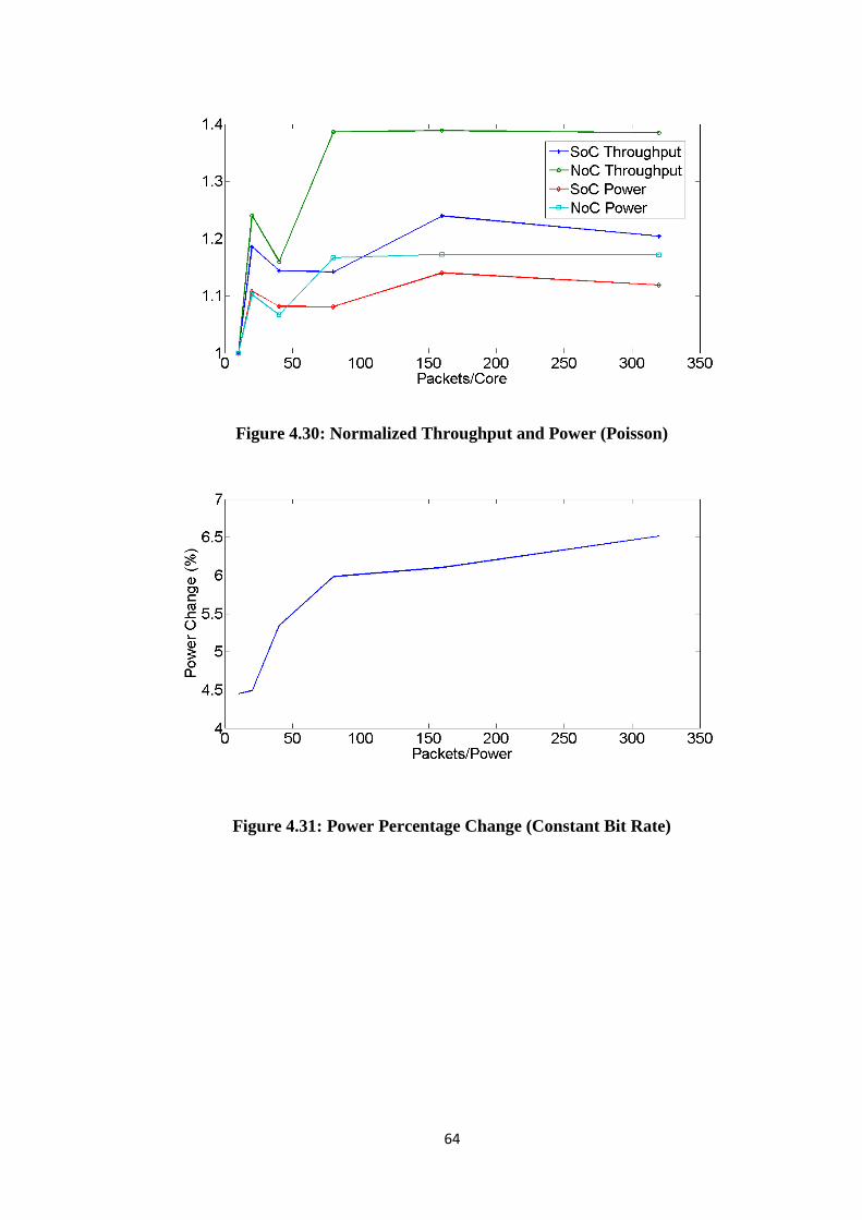
11
Figure 4.30: Normalized Throughput and Power (Poisson)
Figure 4.31: Power Percentage Change (Constant Bit Rate)
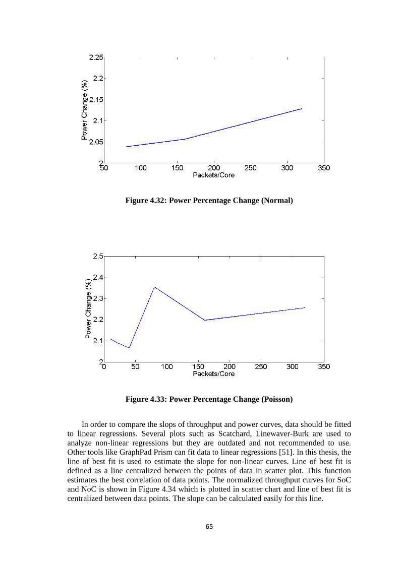
11
Figure 4.32: Power Percentage Change (Normal)
Figure 4.33: Power Percentage Change (Poisson)
In order to compare the slops of throughput and power curves, data should be fitted
to linear regressions. Several plots such as Scatchard, Linewaver-Burk are used to
analyze non-linear regressions but they are outdated and not recommended to use.
Other tools like GraphPad Prism can fit data to linear regressions [51]. In this thesis, the
line of best fit is used to estimate the slope for non-linear curves. Line of best fit is
defined as a line centralized between the points of data in scatter plot. This function
estimates the best correlation of data points. The normalized throughput curves for SoC
and NoC is shown in Figure 4.34 which is plotted in scatter chart and line of best fit is
centralized between data points. The slope can be calculated easily for this line.
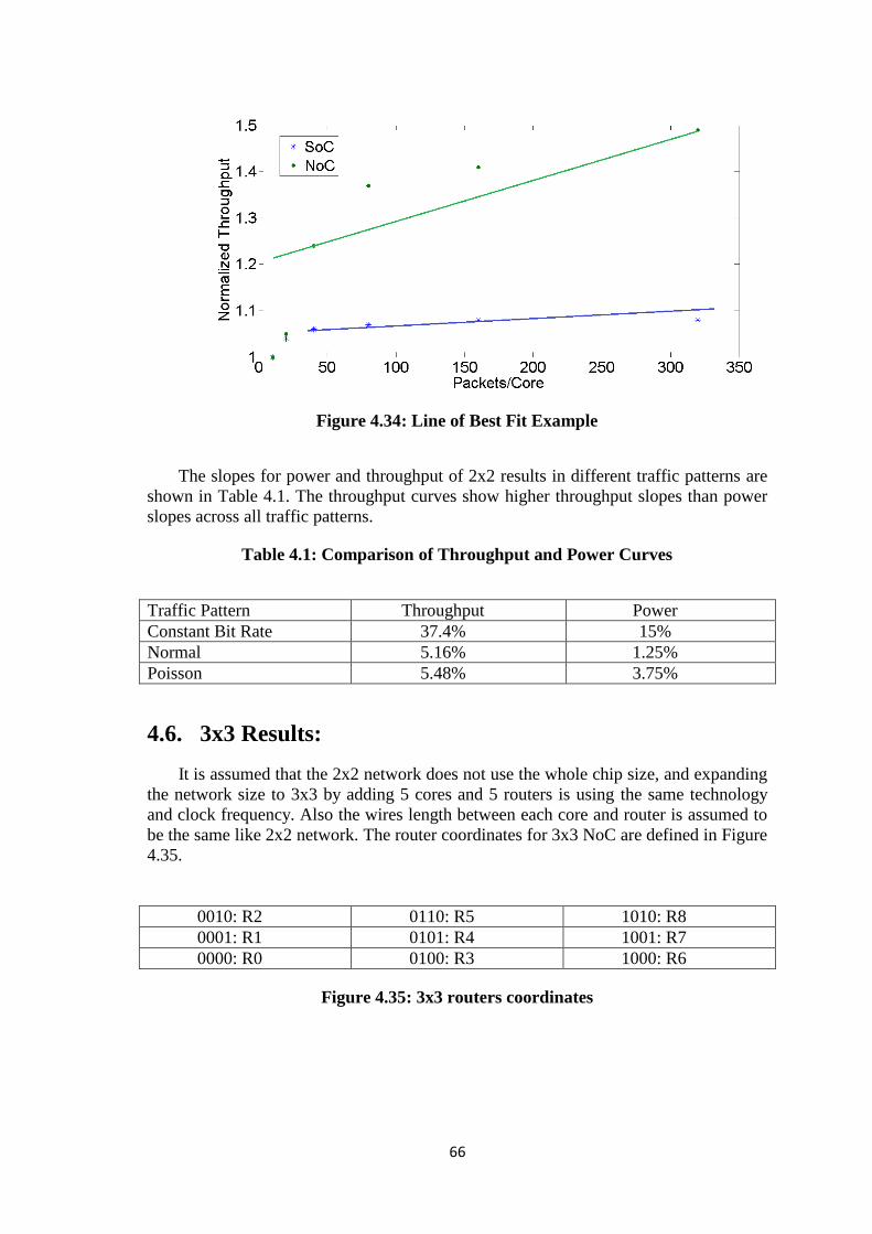
11
Figure 4.34: Line of Best Fit Example
The slopes for power and throughput of 2x2 results in different traffic patterns are
shown in Table 4.1. The throughput curves show higher throughput slopes than power
slopes across all traffic patterns.
Table 4.1: Comparison of Throughput and Power Curves
Traffic Pattern Throughput Power
Constant Bit Rate 37.4% 15%
Normal 5.16% 1.25%
Poisson 5.48% 3.75%
4.6. 3x3 Results:
It is assumed that the 2x2 network does not use the whole chip size, and expanding
the network size to 3x3 by adding 5 cores and 5 routers is using the same technology
and clock frequency. Also the wires length between each core and router is assumed to
be the same like 2x2 network. The router coordinates for 3x3 NoC are defined in Figure
4.35.
0010: R2 0110: R5 1010: R8
0001: R1 0101: R4 1001: R7
0000: R0 0100: R3 1000: R6
Figure 4.35: 3x3 routers coordinates
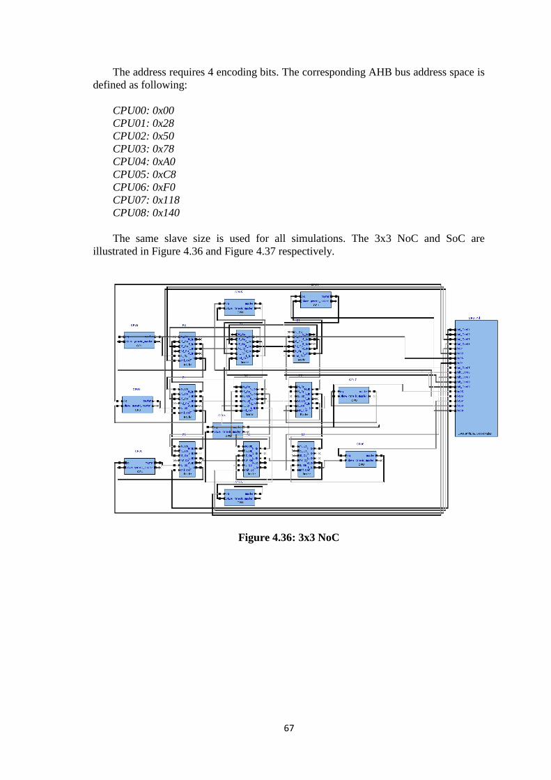
11
The address requires 4 encoding bits. The corresponding AHB bus address space is
defined as following:
CPU00: 0x00
CPU01: 0x28
CPU02: 0x50
CPU03: 0x78
CPU04: 0xA0
CPU05: 0xC8
CPU06: 0xF0
CPU07: 0x118
CPU08: 0x140
The same slave size is used for all simulations. The 3x3 NoC and SoC are
illustrated in Figure 4.36 and Figure 4.37 respectively.
Figure 4.36: 3x3 NoC
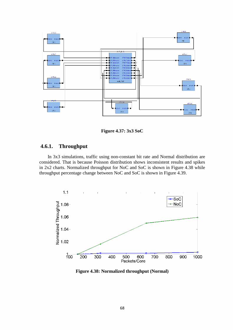
11
Figure 4.37: 3x3 SoC
4.6.1. Throughput
In 3x3 simulations, traffic using non-constant bit rate and Normal distribution are
considered. That is because Poisson distribution shows inconsistent results and spikes
in 2x2 charts. Normalized throughput for NoC and SoC is shown in Figure 4.38 while
throughput percentage change between NoC and SoC is shown in Figure 4.39.
Figure 4.38: Normalized throughput (Normal)
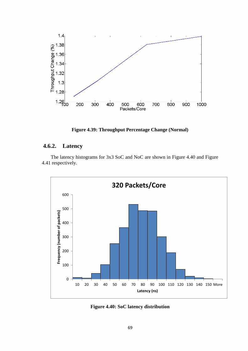
11
Figure 4.39: Throughput Percentage Change (Normal)
4.6.2. Latency
The latency histograms for 3x3 SoC and NoC are shown in Figure 4.40 and Figure
4.41 respectively.
Figure 4.40: SoC latency distribution
0
100
200
300
400
500
600
10 20 30 40 50 60 70 80 90 100 110 120 130 140 150 More
Fre
qu
en
cy (
nu
mb
er
of
pac
kets
)
Latency (ns)
320 Packets/Core
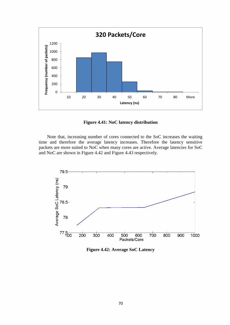
12
Figure 4.41: NoC latency distribution
Note that, increasing number of cores connected to the SoC increases the waiting
time and therefore the average latency increases. Therefore the latency sensitive
packets are more suited to NoC when many cores are active. Average latencies for SoC
and NoC are shown in Figure 4.42 and Figure 4.43 respectively.
Figure 4.42: Average SoC Latency
0
200
400
600
800
1000
1200
10 20 30 40 50 60 70 80 More
Fre
qu
en
cy (
nu
mb
er
of
pac
kets
)
Latency (ns)
320 Packets/Core
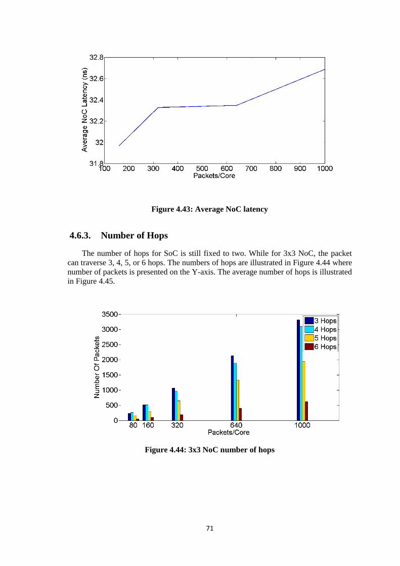
11
Figure 4.43: Average NoC latency
4.6.3. Number of Hops
The number of hops for SoC is still fixed to two. While for 3x3 NoC, the packet
can traverse 3, 4, 5, or 6 hops. The numbers of hops are illustrated in Figure 4.44 where
number of packets is presented on the Y-axis. The average number of hops is illustrated
in Figure 4.45.
Figure 4.44: 3x3 NoC number of hops
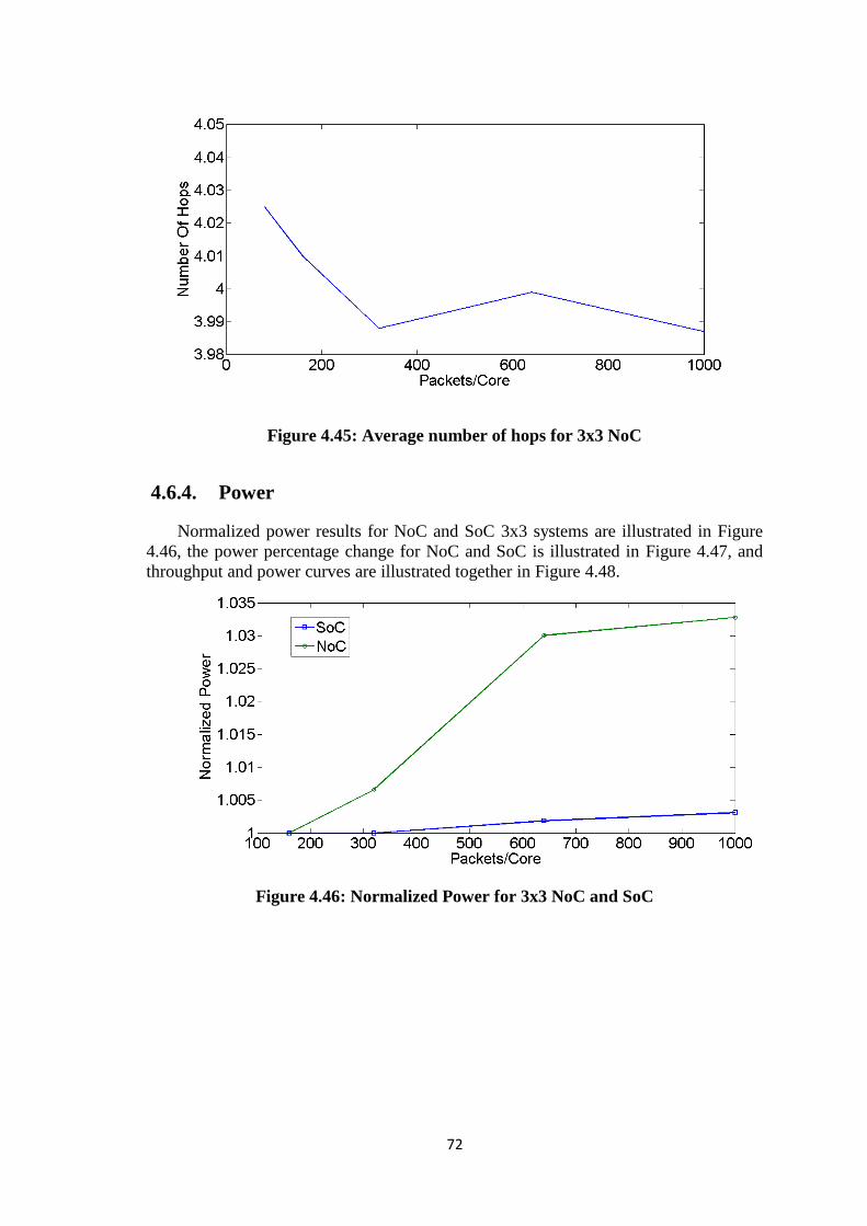
11
Figure 4.45: Average number of hops for 3x3 NoC
4.6.4. Power
Normalized power results for NoC and SoC 3x3 systems are illustrated in Figure
4.46, the power percentage change for NoC and SoC is illustrated in Figure 4.47, and
throughput and power curves are illustrated together in Figure 4.48.
Figure 4.46: Normalized Power for 3x3 NoC and SoC
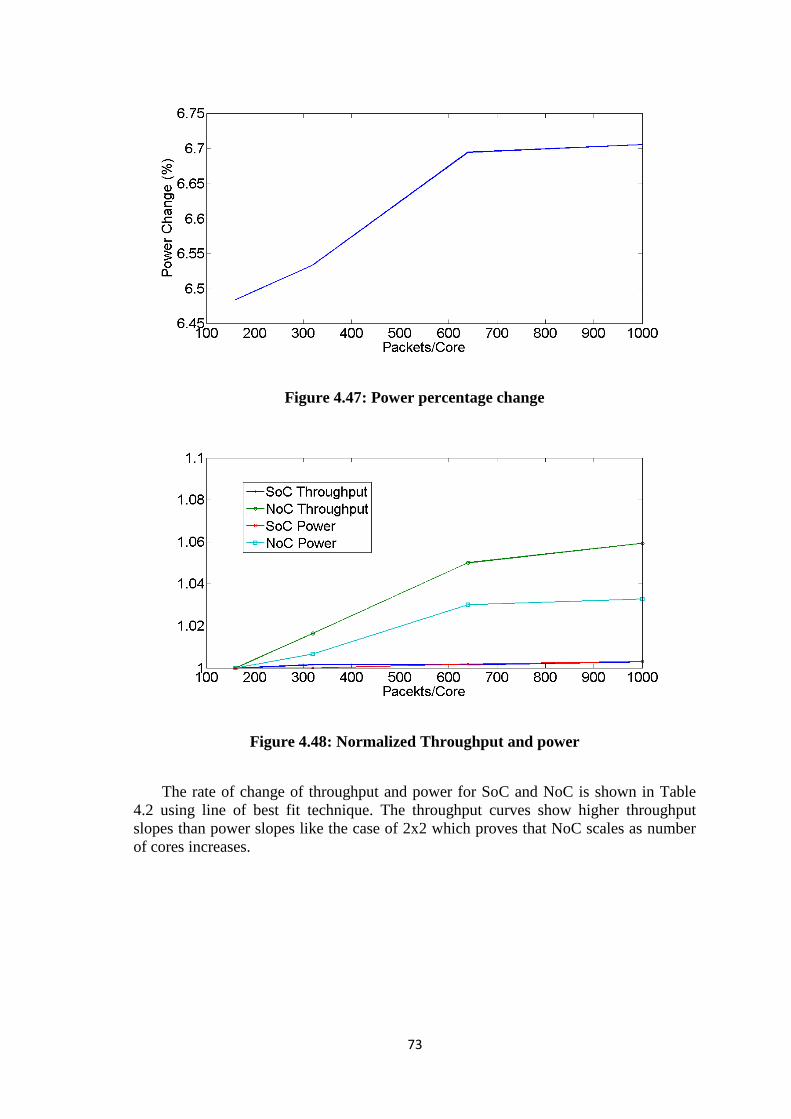
11
Figure 4.47: Power percentage change
Figure 4.48: Normalized Throughput and power
The rate of change of throughput and power for SoC and NoC is shown in Table
4.2 using line of best fit technique. The throughput curves show higher throughput
slopes than power slopes like the case of 2x2 which proves that NoC scales as number
of cores increases.
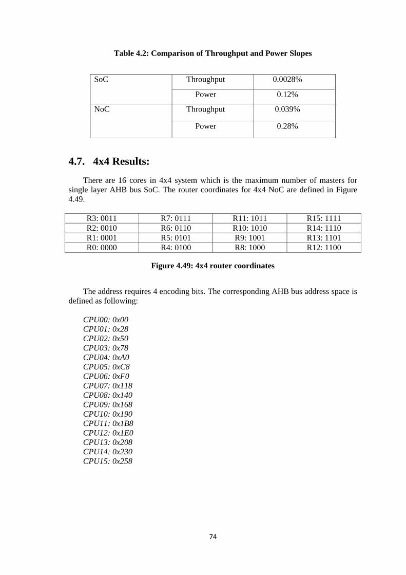
11
Table 4.2: Comparison of Throughput and Power Slopes
SoC Throughput 0.0028%
Power 0.12%
NoC Throughput 0.039%
Power 0.28%
4.7. 4x4 Results:
There are 16 cores in 4x4 system which is the maximum number of masters for
single layer AHB bus SoC. The router coordinates for 4x4 NoC are defined in Figure
4.49.
R3: 0011 R7: 0111 R11: 1011 R15: 1111
R2: 0010 R6: 0110 R10: 1010 R14: 1110
R1: 0001 R5: 0101 R9: 1001 R13: 1101
R0: 0000 R4: 0100 R8: 1000 R12: 1100
Figure 4.49: 4x4 router coordinates
The address requires 4 encoding bits. The corresponding AHB bus address space is
defined as following:
CPU00: 0x00
CPU01: 0x28
CPU02: 0x50
CPU03: 0x78
CPU04: 0xA0
CPU05: 0xC8
CPU06: 0xF0
CPU07: 0x118
CPU08: 0x140
CPU09: 0x168
CPU10: 0x190
CPU11: 0x1B8
CPU12: 0x1E0
CPU13: 0x208
CPU14: 0x230
CPU15: 0x258

11
4.7.1. Throughput
Normalized throughput results for 4x4 systems are illustrated in Figure 4.50.
Throughput percentage change is illustrated Figure 4.51. Similar results are found in
4x4 case and it is noticed that SoC throughput saturates earlier as number of cores
increases.
Figure 4.50: Normalized Throughput (Normal)
Figure 4.51: Throughput Percentage Change (Normal)
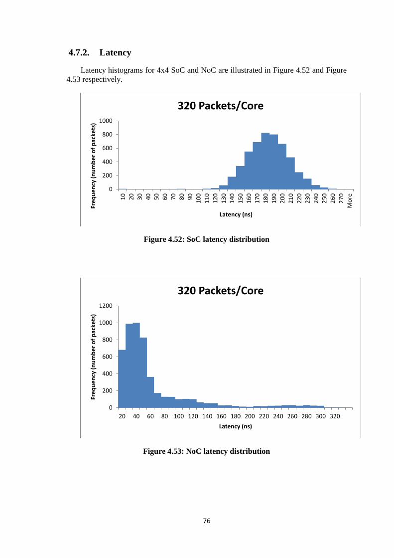
11
4.7.2. Latency
Latency histograms for 4x4 SoC and NoC are illustrated in Figure 4.52 and Figure
4.53 respectively.
Figure 4.52: SoC latency distribution
Figure 4.53: NoC latency distribution
0
200
400
600
800
10001
0
20
30
40
50
60
70
80
90
10
0
11
0
12
0
13
0
14
0
15
0
16
0
17
0
18
0
19
0
20
0
21
0
22
0
23
0
24
0
25
0
26
0
27
0
Mo
re
Fre
qu
en
cy (
nu
mb
er
of
pac
kets
)
Latency (ns)
320 Packets/Core
0
200
400
600
800
1000
1200
20 40 60 80 100 120 140 160 180 200 220 240 260 280 300 320
Fre
qu
en
cy (
nu
mb
er
of
pac
kets
)
Latency (ns)
320 Packets/Core

11
4.7.3. Number of Hops
For 4x4 NoC, the packet can traverse 3 to 8 hops. The numbers of hops are shown
in Figure 4.54 where number of packets is presented on Y-axis. The average number of
hops for NoC is illustrated in Figure 4.55.
Figure 4.54: 4x4 NoC number of hops
Figure 4.55: Average number of hops for 4x4 NoC
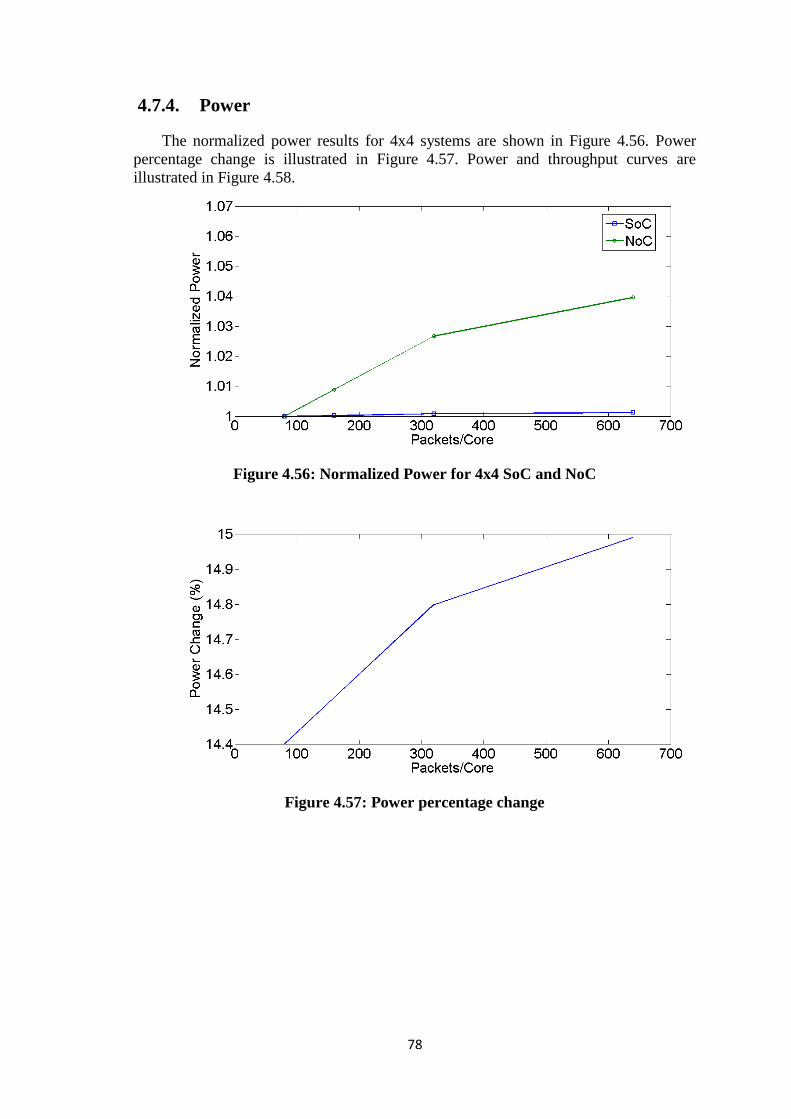
11
4.7.4. Power
The normalized power results for 4x4 systems are shown in Figure 4.56. Power
percentage change is illustrated in Figure 4.57. Power and throughput curves are
illustrated in Figure 4.58.
Figure 4.56: Normalized Power for 4x4 SoC and NoC
Figure 4.57: Power percentage change

11
Figure 4.58: Normalized Throughput and power
The rate of change for throughput and power are shown in Table 4.3. Like 2x2 and
3x3, the throughput slope is higher than power slope for NoC and SoC.
Table 4.3: Comparison of Throughput and Power Slopes
SoC Throughput 0.0032%
Power 0.16%
NoC Throughput 0.045%
Power 0.31%
12
Discussion and Conclusions
As number of Cores in SoC is increasing, NoC design paradigm dominates the SoC
development. This thesis implements TLM models for NoC and SoC (using shared bus
AHB protocol). TLM offers some capabilities like easy and fast development in
addition to evaluation of performance metrics like throughput which is best calculated
on transaction level. Different traffic patterns were examined such as constant bit rate,
non-constant bit rate in addition to some random patterns such as uniform, normal, and
Poisson. Different performance metrics are used for evaluation such as throughput,
latency, number of hops, and power. The power-throughput is the best representation of
cost performance problem for NoC design. The simulations examined different network
sizes and traffic loads. The results show that NoC outperforms SoC as traffic load
increases or number of cores increases. This is due to the multi-access shared buses
limitations. On the other hand, NoC shows higher power consumption due to larger
number of transactions but still the rate of change of throughput is higher than that of
power. Regarding latency, the SoC offers lower latencies for small number of cores
which is suitable for latency sensitive packets in system with limited number of cores.
When number of cores increases, the NoC outperforms SoC with low average latency.
11
Future Work
As network topology affects performance, the future work includes carrying the
same experiments on different topologies rather than mesh. The same concept applies
on routing algorithms; other adaptive routing algorithms can be tested. On the other
hand, the tested SoC used shared buses implementing AHB protocol. The AXI protocol
is another example for shared buses medium which is expected to show better results as
it supports multi-access for different masters with the same priority. The future work
also includes building RTL models for NoC and SoC and comparing RLT with TLM
models.

11
References
1. Sheibanyrad, A; Miro Panades, I; Greiner, A, "Systematic Comparison between the
Asynchronous and the Multi-Synchronous Implementations of a Network on Chip
Architecture," Design, Automation & Test in Europe Conference & Exhibition,
2007. DATE '07 , vol., no., pp.1,6, 16-20 April 2007
2. Benini, L.; De Micheli, G., "Networks on chips: a new SoC paradigm," Computer ,
vol.35, no.1, pp.70,78, Jan 2002
3. Pande, P.P.; Grecu, C.; Ivanov, A; Saleh, R., "High-throughput switch-based
interconnect for future SoCs," System-on-Chip for Real-Time Applications, 2003.
Proceedings. The 3rd IEEE International Workshop on , vol., no., pp.304,310, 30
June-2 July 2003
4. Mello, A; Tedesco, L.; Calazans, N.; Moraes, F., "Virtual Channels in Networks on
Chip: Implementation and Evaluation on Hermes NoC," Integrated Circuits and
Systems Design, 18th Symposium on , vol., no., pp.178,183, 4-7 Sept. 2005
5. Bononi, L.; Concer, N.; Grammatikakis, M.; Coppola, M.; Locatelli, R., "NoC
Topologies Exploration based on Mapping and Simulation Models," Digital System
Design Architectures, Methods and Tools, 2007. DSD 2007. 10th Euromicro
Conference on , vol., no., pp.543,546, 29-31 Aug. 2007
6. Dally, W.J., "Virtual-channel flow control," Computer Architecture, 1990.
Proceedings., 17th Annual International Symposium on , vol., no., pp.60,68, 28-31
May 1990
7. Chouchene, W.; Attia, B.; Zitouni, A; Abid, N.; Tourki, R., "A low power network
interface for network on chip," Systems, Signals and Devices (SSD), 2011 8th
International Multi-Conference on , vol., no., pp.1,6, 22-25 March 2011
8. Nan Ni; Pirvu, M.; Laxmi Bhuyan, "Circular buffered switch design with wormhole
routing and virtual channels," Computer Design: VLSI in Computers and
Processors, 1998. ICCD '98. Proceedings. International Conference on , vol., no.,
pp.466,473, 5-7 Oct 1998
9. Tamir Y.; Frazier G. L., “High-performance multi-queue buffers for VLSI
communications switches,” ISCA '88 Proceedings of the 15th Annual International
Symposium on Computer architecture, 1988.
10. Nicopoulos, C.A; Dongkook Park; Jongman Kim; Vijaykrishnan, N.; Yousif, M.S.;
Das, C.R., "ViChaR: A Dynamic Virtual Channel Regulator for Network-on-Chip
Routers," Microarchitecture, 2006. MICRO-39. 39th Annual IEEE/ACM
International Symposium on , vol., no., pp.333,346, 9-13 Dec. 2006
11. Rabab Ezz-Eldin Rabea, “HIGH-PERFORMANCE AND LOW-POWER
NETWORK ON CHIP SWITCH,” Master of Science thesis.
12. Sayed Taha Muhammed, “NOC SWITCH TRAFFIC SIMULATION AND
PERFORMANCE ENHANCEMENT,” Master of Science thesis
11
13. Pande, P.P.; Grecu, C.; Jones, M.; Ivanov, A; Saleh, R., "Effect of traffic
localization on energy dissipation in NoC-based interconnect," Circuits and
Systems, 2005. ISCAS 2005. IEEE International Symposium on , vol., no.,
pp.1774,1777 Vol. 2, 23-26 May 2005
14. Mubeen, S.; Kumar, S., "Designing Efficient Source Routing for Mesh Topology
Network on Chip Platforms," Digital System Design: Architectures, Methods and
Tools (DSD), 2010 13th Euromicro Conference on , vol., no., pp.181,188, 1-3 Sept.
2010
15. Manevich, R.; Cidon, I; Kolodny, A; Walter, I, "Centralized Adaptive Routing for
NoCs," Computer Architecture Letters , vol.9, no.2, pp.57,60, Feb. 2010
16. Sheng-guang Yang; Li Li; Yu-ang Zhang; Bing Zhang; Yi Xu, "A power-aware
adaptive routing scheme for network on a chip," ASIC, 2007. ASICON '07. 7th
International Conference on , vol., no., pp.1301,1304, 22-25 Oct. 2007
17. Wang Zhang; Ligang Hou; Jinhui Wang; Shuqin Geng; Wuchen Wu, "Comparison
Research between XY and Odd-Even Routing Algorithm of a 2-Dimension 3X3
Mesh Topology Network-on-Chip," Intelligent Systems, 2009. GCIS '09. WRI
Global Congress on , vol.3, no., pp.329,333, 19-21 May 2009
18. Mejia, A; Flich, J.; Duato, J., "On the Potentials of Segment-Based Routing for
NoCs," Parallel Processing, 2008. ICPP '08. 37th International Conference on , vol.,
no., pp.594,603, 9-12 Sept. 2008
19. Mejia, A; Palesi, M.; Flich, J.; Kumar, S.; Lopez, P.; Holsmark, R.; Duato, J.,
"Region-Based Routing: A Mechanism to Support Efficient Routing Algorithms in
NoCs," Very Large Scale Integration (VLSI) Systems, IEEE Transactions on ,
vol.17, no.3, pp.356,369, March 2009
20. Palesi, M.; Holsmark, R.; Kumar, S.; Catania, V., "Application Specific Routing
Algorithms for Networks on Chip," Parallel and Distributed Systems, IEEE
Transactions on , vol.20, no.3, pp.316,330, March 2009
21. Moreno, E.I; Marcon, C.AM.; Calazans, N. L V; Moraes, F.G., "Arbitration and
routing impact on NoC design," Rapid System Prototyping (RSP), 2011 22nd IEEE
International Symposium on , vol., no., pp.193,198, 24-27 May 2011
22. Salminen, E.; Kulmala, A; Hamalainen, T.D., "On network-on-chip comparison,"
Digital System Design Architectures, Methods and Tools, 2007. DSD 2007. 10th
Euromicro Conference on , vol., no., pp.503,510, 29-31 Aug. 2007
23. Harmanci, M.D.; Escudero, N.P.; Leblebici, Y.; Ienne, P., "Quantitative modelling
and comparison of communication schemes to guarantee quality-of-service in
networks-on-chip," Circuits and Systems, 2005. ISCAS 2005. IEEE International
Symposium on , vol., no., pp.1782,1785 Vol. 2, 23-26 May 2005
24. Sahu, S.; Kittur, H.M., "Area and power efficient network on chip router
architecture," Information & Communication Technologies (ICT), 2013 IEEE
Conference on , vol., no., pp.855,859, 11-12 April 2013
25. Bartels, C.; Huisken, J.; Goossens, K.; Groeneveld, P.; van Meerbergen, J.,
"Comparison of An Æthereal Network on Chip and A Traditional Interconnect for
A Multi-Processor DVB-T System on Chip," Very Large Scale Integration, 2006
IFIP International Conference on , vol., no., pp.80,85, 16-18 Oct. 2006

11
26. Manevich, R.; Walter, I; Cidon, I; Kolodny, A, "Best of both worlds: A bus
enhanced NoC (BENoC)," Electrical and Electronics Engineers in Israel (IEEEI),
2010 IEEE 26th Convention of , vol., no., pp.000876,000880, 17-20 Nov. 2010
27. Ling Wang; Jianye Hao; Feixuan Wang, "Bus-Based and NoC Infrastructure
Performance Emulation and Comparison," Information Technology: New
Generations, 2009. ITNG '09. Sixth International Conference on , vol., no.,
pp.855,858, 27-29 April 2009
28. Vainbrand, D.; Ginosar, R., "Comparing NoC architectures for neural networks,"
Electrical and Electronics Engineers in Israel (IEEEI), 2010 IEEE 26th Convention
of , vol., no., pp.000660,000664, 17-20 Nov. 2010
29. Grötker, T.; Liao, S.; Martin, G.; Swan, S., “System Design with SystemC,”
Hingham, MA, USA: Kluwer Academic Publishers, 2002
30. Mentor Graphics Vista Modeling Guide
31. ARM AMBA Specification (Rev 2.0)
32. Mentor Graphics Vista Tutorial
33. Sungho Park, “A VERIOG-HDL IMPLEMENTATION OF VIRTUAL
CHANNELS IN A NETWORK-ON-CHIP ROUTER,” Master of Science thesis
34. Mentor Graphics Vista User’s Manual
35. Leary, G.; Chatha, K.S., "Design of NoC for SoC with Multiple Use Cases
Requiring Guaranteed Performance," VLSI Design, 2010. VLSID '10. 23rd
International Conference on , vol., no., pp.200,205, 3-7 Jan. 2010
36. Kangmin Lee; Se-Joong Lee; Hoi-Jun Yoo, "Low-power network-on-chip for high-
performance SoC design," Very Large Scale Integration (VLSI) Systems, IEEE
Transactions on , vol.14, no.2, pp.148,160, Feb. 2006
37. Murali, S.; Atienza, D.; Meloni, P.; Carta, Salvatore; Benini, L.; De Micheli, G.;
Raffo, L., "Synthesis of Predictable Networks-on-Chip-Based Interconnect
Architectures for Chip Multiprocessors," Very Large Scale Integration (VLSI)
Systems, IEEE Transactions on , vol.15, no.8, pp.869,880, Aug. 2007
38. Mahadevan, S.; Angiolini, F.; Storoaard, M.; Olsen, R.G.; Sparsoe, J.; Madsen, J.,
"Network traffic generator model for fast network-on-chip simulation," Design,
Automation and Test in Europe, 2005. Proceedings , vol., no., pp.780,785 Vol. 2, 7-
11 March 2005
39. Zhonghai Lu; Jantsch, A, "Traffic configuration for evaluating networks on chips,"
System-on-Chip for Real-Time Applications, 2005. Proceedings. Fifth International
Workshop on , vol., no., pp.535,540, 20-24 July 2005
40. Hai-Hua Wen; Gao-Ming Du; Duo-li Zhang; Luo-Feng Geng; Ming-Lun Gao;
Ying-Chun Chen, "Design of an on-line configurable traffic generator for NoC,"
Anti-counterfeiting, Security, and Identification in Communication, 2009. ASID
2009. 3rd International Conference on , vol., no., pp.556,559, 20-22 Aug. 2009
41. Tedesco, L.; Mello, A; Garibotti, D.; Calazans, N.; Moraes, F., "Traffic Generation
and Performance Evaluation for Mesh-based NoCs," Integrated Circuits and
Systems Design, 18th Symposium on , vol., no., pp.184,189, 4-7 Sept. 2005
11
42. Grecu, C.; Ivanov, A; Saleh, R.; Rusu, C.; Anghel, L.; Pande, P.P.; Nuca, V., "A
flexible network-on-chip simulator for early design space exploration,"
Microsystems and Nanoelectronics Research Conference, 2008. MNRC 2008. 1st ,
vol., no., pp.33,36, 15-15 Oct. 2008
43. Weichen Liu; Jiang Xu; Xiaowen Wu; Yaoyao Ye; Xuan Wang; Wei Zhang;
Nikdast, M.; Zhehui Wang, "A NoC Traffic Suite Based on Real Applications,"
VLSI (ISVLSI), 2011 IEEE Computer Society Annual Symposium on , vol., no.,
pp.66,71, 4-6 July 2011
44. Ost, L.; Mello, A; Palma, J.; Moraes, F.; Calazans, N., "MAIA - a framework for
networks on chip generation and verification," Design Automation Conference,
2005. Proceedings of the ASP-DAC 2005. Asia and South Pacific , vol.1, no.,
pp.49,52 Vol. 1, 18-21 Jan. 2005
45. Soteriou, V.; Hangsheng Wang; Li-Shiuan Peh, "A Statistical Traffic Model for
On-Chip Interconnection Networks," Modeling, Analysis, and Simulation of
Computer and Telecommunication Systems, 2006. MASCOTS 2006. 14th IEEE
International Symposium on , vol., no., pp.104,116, 11-14 Sept. 2006
46. Pekkarinen, E.; Lehtonen, L.; Salminen, E.; Hamalainen, T.D., "A set of traffic
models for Network-on-Chip benchmarking," System on Chip (SoC), 2011
International Symposium on , vol., no., pp.78,81, Oct. 31 2011-Nov. 2 2011
47. Antichi, G.; Di Pietro, A; Ficara, D.; Giordano, S.; Procissi, G.; Vitucci, F.,
"Design of a High Performance Traffic Generator on Network Processor," Digital
System Design Architectures, Methods and Tools, 2008. DSD '08. 11th
EUROMICRO Conference on , vol., no., pp.438,441, 3-5 Sept. 2008
48. Lahiri, K.; Raghunathan, A; Dey, S., "Evaluation of the traffic-performance
characteristics of system-on-chip communication architectures," VLSI Design,
2001. Fourteenth International Conference on , vol., no., pp.29,35, 2001
49. William James Dally, Brian Towles, "Principles and Practices of Interconnection
Networks", Morgan Kaufmann, 2004
50. Pande, P.P.; Grecu, C.; Jones, M.; Ivanov, A; Saleh, R., "Performance evaluation
and design trade-offs for network-on-chip interconnect architectures," Computers,
IEEE Transactions on , vol.54, no.8, pp.1025,1040, Aug. 2005
51. Harvey Motulsky; Arthur Christopoulos, “Fitting Models to Biological Data using
Linear and Nonlinear Regression,” GraphPad PRISM, Version 4.0

11
Appendix A: SystemC Code for Router Model
//Defined function for comparing coordinates of packet and current router
char Router_pv::compare_coordinates (unsigned short coordinates) {
cout << name() << "@" << sc_time_stamp() << " Comparing Coordinates:
" << coordinates << endl;
sc_uint<16> cord = coordinates;
unsigned short cordx = cord.range(3, 2);
unsigned short cordy = cord.range(1, 0);
cout << name() << "@" << sc_time_stamp() << " Router Coordinates: "
<< Router_Coordinates << endl;
Cx_Cy = Router_Coordinates;
unsigned short Cx = Cx_Cy.range(3, 2);
unsigned short Cy = Cx_Cy.range(1, 0);
if (cordx > Cx) {
return 'E';
} else if (cordx < Cx) {
return 'W';
} else {
if (cordy < Cy) {
return 'S';
} else if (cordy > Cy) {
return 'N';
} else {
return 'C';
}
}
}
// Defined function for sending data on any input port
void Router_pv::send_data(unsigned int data) {
cout << name() << "@" << sc_time_stamp() << " Sending Data: " << data
<< endl;
sc_uint<32> dat = data;
char dest_port;
unsigned short coordinates;
coordinates = dat.range(19, 16);
dest_port = compare_coordinates(coordinates);
cout << name() << "@" << sc_time_stamp() << " Destination port is: " <<
dest_port << endl;
unsigned int key = data;
ofstream hops_list;
ofstream data_list;
hops_list.open("hops_list.txt", std::ios::app);
data_list.open("data_list.txt", std::ios::app);
if (dest_port == 'N') {
N_Ip_write (0, data);
hops[key] += 1;
11
} else if (dest_port == 'S') {
S_Ip_write (0, data);
hops[key] += 1;
} else if (dest_port == 'W') {
W_Ip_write (0, data);
hops[key] += 1;
} else if (dest_port == 'E') {
E_Ip_write (0, data);
hops[key] += 1;
} else if (dest_port == 'C') {
L_Ip_write (0, data);
hops[key] += 1;
hops_list << hops[key] << endl;
data_list << data << endl;
}
}
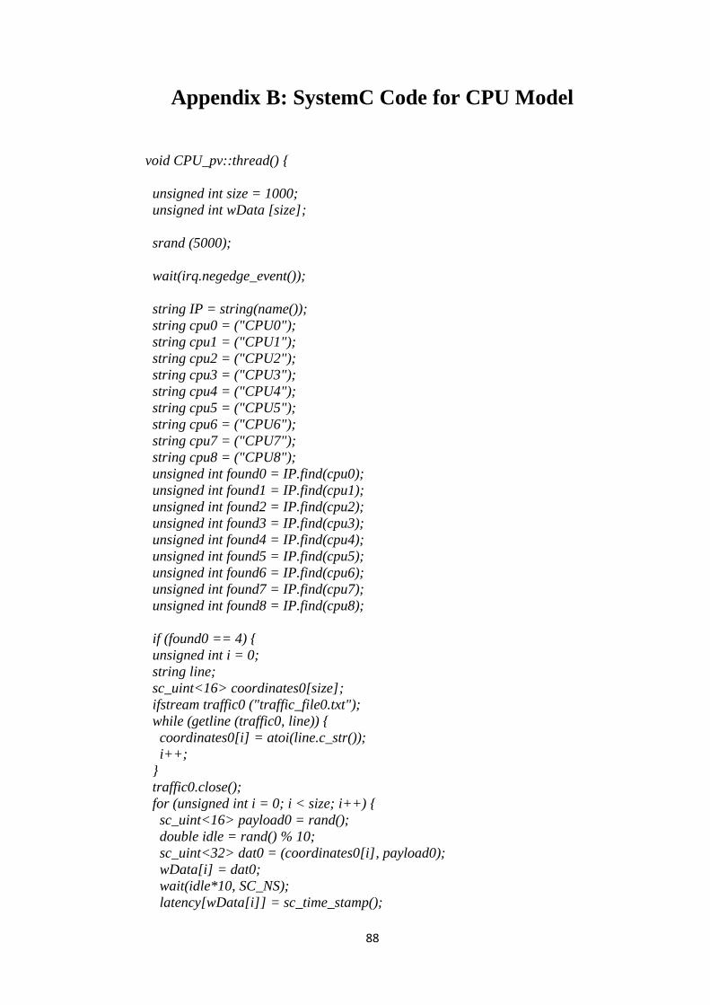
11
Appendix B: SystemC Code for CPU Model
void CPU_pv::thread() {
unsigned int size = 1000;
unsigned int wData [size];
srand (5000);
wait(irq.negedge_event());
string IP = string(name());
string cpu0 = ("CPU0");
string cpu1 = ("CPU1");
string cpu2 = ("CPU2");
string cpu3 = ("CPU3");
string cpu4 = ("CPU4");
string cpu5 = ("CPU5");
string cpu6 = ("CPU6");
string cpu7 = ("CPU7");
string cpu8 = ("CPU8");
unsigned int found0 = IP.find(cpu0);
unsigned int found1 = IP.find(cpu1);
unsigned int found2 = IP.find(cpu2);
unsigned int found3 = IP.find(cpu3);
unsigned int found4 = IP.find(cpu4);
unsigned int found5 = IP.find(cpu5);
unsigned int found6 = IP.find(cpu6);
unsigned int found7 = IP.find(cpu7);
unsigned int found8 = IP.find(cpu8);
if (found0 == 4) {
unsigned int i = 0;
string line;
sc_uint<16> coordinates0[size];
ifstream traffic0 ("traffic_file0.txt");
while (getline (traffic0, line)) {
coordinates0[i] = atoi(line.c_str());
i++;
}
traffic0.close();
for (unsigned int i = 0; i < size; i++) {
sc_uint<16> payload0 = rand();
double idle = rand() % 10;
sc_uint<32> dat0 = (coordinates0[i], payload0);
wData[i] = dat0;
wait(idle*10, SC_NS);
latency[wData[i]] = sc_time_stamp();

11
cout << name() << "@" << sc_time_stamp() << "(" << dec <<
sc_delta_count() << ") Sending Data wData[" << i << "]" << wData[i] << endl;
master_write(0, wData[i]);
}
}

94
Appendix C: C Code for Traffic Generation
#include <iostream>
#include <fstream>
#include <random>
using namespace std;
int main () {
int size = 2000;
std::default_random_engine generator;
std::normal_distribution<double> distribution(180,180);
ofstream traffic0;
traffic0.open("traffic_random0.txt");
for (unsigned int i = 0; i < size; i++) {
unsigned int addr0 = distribution(generator);
if (addr0 > 359) addr0 = 359;
else if (addr0 < 40) addr0 = 40;
traffic0 << addr0 << endl;
}
traffic0.close();

94
Publication
Amr Hany, Magdy A. El-Moursy, Hossam A. H. Fahmy, “Network Of Cores For
Large Systems, ” In The Proceedings of IEEE International Conference on Computer
Engineering and Systems, December 2014.

94
ملخصال
تم عمل مقارنة بين أنظمة و شبكات الرقائق االلكترونية عن طريق نمذجة كل منهم على التوجيه فى عدة أمثلة لشبكات ذات احجام مختلفة. تم تنفيذ نموذج جهاز المستوى االجرائى.
ايضا تمت تجربة عدة أنماط و أحمال مختلفة للبيانات المرسلة عبر الشبكة. تم تقييم اداء النظم و الشبكات تفصيليا باستخدام عدة مقاييس مثل االنتاجية و معدل استهالك الطاقة. أوضحت
النسبة لالنتاجية و بمعدل زيادة اعلى من معدل زيادة النتائج تفوق شبكات الرقائق االلكترونية ب استهالك الطاقة كلما زاد حجم الشبكة.

عمرو أحمد هانى محمد عبد القادر أحمد سالم :دسـمهن 2801\80\12 تاريخ الميالد:
مصرى الجنسية: 1888\28\2 تاريخ التسجيل:
..........\....\.... تاريخ المنح: االلكترونيات و االتصاالت الكهربيةهندسة القسم: العلوم ماجستير الدرجة:
المشرفون: حسام على حسن فهمىد.
معهد بحوث , , قسم االلكترونيات الدقيقةمجدى على على المرسىد. االلكترونيات
الممتحنون: فهمىحسام على حسن د.
معهد بحوث , مجدى على على المرسى, قسم االلكترونيات الدقيقةد. االلكترونيات
د. تامر فريد البط . محمد أمين دسوقى, كلية الهندسة, جامعة عين شمسأ.د
عنوان الرسالة: نمذجة على المستوى االجرائى لشبكات و نظم الرقائق االلكترونية
الكلمات الدالة:
نمذجة على المستوى االجرائى, شبكات الرقائق االكترونية, نظم الرقائق االلكترونية
:رسالةملخـص التم عمل مقارنة بين أنظمة و شبكات الرقائق االلكترونية عن طريق نمذجة كل منهم
لشبكات ذات على المستوى االجرائى. تم تنفيذ نموذج جهاز التوجيه فى عدة أمثلةاحجام مختلفة. ايضا تمت تجربة عدة أنماط و أحمال مختلفة للبيانات المرسلة عبر الشبكة. تم تقييم اداء النظم و الشبكات تفصيليا باستخدام عدة مقاييس مثل االنتاجية و معدل استهالك الطاقة. أوضحت النتائج تفوق شبكات الرقائق االلكترونية بالنسبة
معدل زيادة اعلى من معدل زيادة استهالك الطاقة كلما زاد حجم الشبكة.لالنتاجية و ب
ضع صورتك هنا

نمذجة على المستوى االجرائى لشبكات و نظم الرقائق االلكترونية
اعداد
عمرو أحمد هانى محمد
القاهرة جامعة - الهندسة كلية إلى مقدمة رسالة
العلوم ماجستير درجة على الحصول متطلبات من كجزء
في
االلكترونيات و االتصاالت الكهربيةهندسة
:يعتمد من لجنة الممتحنين
الدكتور: حسام على حسن فهمى المشرف الرئيسى
, قسم االلكترونيات الدكتور: مجدى على على المرسى عضو
الدقيقة, معهد بحوث االلكترونيات
الممتحن الداخلى البطتامر فريد الدكتور:
, كلية الهندسة, خارجىالممتحن ال دسوقى محمد أمين االستاذ الدكتور:
جامعة عين شمس
القاهــرة جامعــة - الهندســة كليــة
العربيــة مصـر جمهوريـة - الجيـزة
1025

و نظم الرقائق االلكترونية نمذجة على المستوى االجرائى لشبكات
اعداد
عمرو أحمد هانى محمد
القاهرة جامعة - الهندسة كلية إلى مقدمة رسالة
العلوم ماجستير درجة على الحصول متطلبات من كجزء
في
االلكترونيات و االتصاالت الكهربيةهندسة
تحت اشراف
د. حسام على حسن فهمى د. مجدى على على المرسى
استاذ مساعد بقسم االلكترونيات
الدقيقة معهد بحوث االلكترونيات
بالقاهرة
استاذ مساعد بقسم االلكترونيات و
االتصاالت كلية الهندسة جامعة
القاهرة
القاهــرة جامعــة - الهندســة كليــة
العربيــة مصـر جمهوريـة - الجيـزة
1025

االجرائى لشبكات و نظم الرقائق االلكترونيةنمذجة على المستوى
اعداد
عمرو أحمد هانى محمد
القاهرة جامعة - الهندسة كلية إلى مقدمة رسالة
العلومماجستير درجة على الحصول متطلبات من كجزء
في
االلكترونيات و االتصاالت الكهربيةهندسة
القاهــرة جامعــة - الهندســة كليــة
العربيــة مصـر جمهوريـة - الجيـزة
1025