tramp ship routing and scheduling - models, methods...
TRANSCRIPT
General rights Copyright and moral rights for the publications made accessible in the public portal are retained by the authors and/or other copyright owners and it is a condition of accessing publications that users recognise and abide by the legal requirements associated with these rights.
• Users may download and print one copy of any publication from the public portal for the purpose of private study or research. • You may not further distribute the material or use it for any profit-making activity or commercial gain • You may freely distribute the URL identifying the publication in the public portal
If you believe that this document breaches copyright please contact us providing details, and we will remove access to the work immediately and investigate your claim.
Downloaded from orbit.dtu.dk on: Jun 29, 2018
Tramp Ship Routing and Scheduling - Models, Methods and Opportunities
Vilhelmsen, Charlotte; Larsen, Jesper; Lusby, Richard Martin
Publication date:2015
Document VersionPeer reviewed version
Link back to DTU Orbit
Citation (APA):Vilhelmsen, C., Larsen, J., & Lusby, R. M. (2015). Tramp Ship Routing and Scheduling - Models, Methods andOpportunities. DTU Management Engineering.
Tramp Ship Routing and Scheduling
- Models, Methods and Opportunities
Charlotte Vilhelmsen Jesper Larsen Richard M. Lusby
Department of Management Engineering, Technical University of Denmark
Produktionstorvet, Building 426, 2800 Kgs. Lyngby, Denmark
[email protected], [email protected], [email protected]
November 13, 2015
Abstract
In tramp shipping, ships operate much like taxies, following the available demand. Thiscontrasts liner shipping where vessels operate more like busses on a fixed route network ac-cording to a published timetable. Tramp operators can enter into long term contracts andthereby determine some of their demand in advance. However, the detailed requirements ofthese contract cargoes can be subject to ongoing changes, e.g. the destination port can bealtered. For tramp operators, a main concern is therefore the efficient and continuous planningof routes and schedules for the individual ships. Due to mergers, pooling, and collaboration ef-forts between shipping companies, the fleet sizes have grown to a point where manual planningis no longer adequate in a market with tough competition and low freight rates.
The aim of this paper is to provide a comprehensive introduction to tramp ship routingand scheduling. This includes a review on existing literature, modelling approaches, solu-tion methods as well as an analysis of the current status and future opportunities of researchwithin tramp ship routing and scheduling. We argue that rather than developing new solu-tion methods for the basic routing and scheduling problem, focus should now be on extendingthis basic problem to include additional real-world complexities and develop suitable solutionmethods for those extensions. Such extensions will enable more tramp operators to bene-fit from the solution methods while simultaneously creating new opportunities for operatorsalready benefitting from existing methods.
1 Introduction
In 2013, global seaborne trade was estimated to have reached nearly 9.6 billion tons (UNCTAD,2014). This translates into well over a tonne of cargo for every single individual on the planet, ev-ery single year, or equivalently around 90% of world trade by volume (ICS). World trade thereforedepends on the international shipping industry’s efficiency and competitive freight rates. Further-more, even though international shipping is the most carbon efficient mode of transport, the CO2
emissions from the industry as a whole are still estimated to be around 2.2% of current globalemissions (ICS) adding further incentive to improve efficiency within the industry. For severalyears now, the maritime sector has been subject to low freight rates caused by surplus fleet ca-pacity and the weak economy. The combination of low freight rates and high bunker oil priceshas made it difficult for many operators to produce earnings sufficient to cover just their min-imum operating costs. The shipping industry itself, therefore, has as much incentive as any to
1
2 1. Introduction
improve their cost-effectiveness and recent years have shown increased exploration of strategies inthis direction, e.g. slow steaming, which refers to the practice of operating ships at reduced speedsin order to save fuel. At the same time, the maritime sector also has an incentive to take theirCO2 emissions into consideration, both due to political pressure and to the fact that the industryitself is bound to be affected by the impacts of climate change, such as rising sea levels and moreextreme weather. From all sides there is therefore an interest in research to increase efficiencywithin maritime transportation.
Within commercial shipping it is common to distinguish between three different basic operatingmodes although they need not be mutually exclusive: liner, tramp and industrial (Lawrence, 1972).Within liner shipping, which is primarily characterised by container shipping, vessels operate muchlike busses on a fixed route network according to a published timetable. In contrast, tramp shipsoperate much more like taxies following the available cargoes. Many tramp operators do howeverknow some of the demand in advance as they can enter into long term agreements called contractsof affreightment (CoAs). Such contracts state that the tramp operator is obliged to transportspecified quantities of cargo between specified ports at a given rate during a specified time period.In addition to these contract cargoes, a tramp operator then tries to maximise profit from optionalcargoes called spot cargoes. In industrial shipping, the ship operator is also the cargo owner andthe objective is therefore to carry all the predefined cargoes at the minimum cost. Tramp andindustrial shipping are primarily characterised by tankers and dry bulk carriers.
UNCTAD (2014) reports that although it is estimated that more than half of seaborne tradein dollar terms is containerised, this segment only accounts for 16% of global seaborne tradeby volume. Furthermore, container ships only account for 13% of the world fleet deadweighttonnage while bulk carriers and oil tankers are responsible for respectively 43% and 29%. Similarly,UNCTAD (2013) reports that in 2012, bulk commodities accounted for nearly three quarters ofthe total ton-miles performed that year. Tramp and industrial operators are therefore accountablefor a massive part of the global fleet as well as the total ton-miles performed each year, and henceeven small improvements in efficiency within these operating modes can be expected to have greatimpact from both an economic and an environmental aspect.
As such, tramp shipping is not characterised by large economies of scale. Therefore, thisshipping mode is generally not difficult to enter and has previously been comprised of many smalloperators. Perhaps this is the reason why research within tramp shipping has previously lagged farbehind that of industrial shipping (Christiansen et al., 2004). However, recent trends of mergers,pooling, and collaboration efforts between shipping companies have increased fleet sizes to a pointwhere manual planning is no longer adequate (Christiansen et al., 2004). A further motivation forresearch within tramp shipping is that many companies previously involved in industrial shippinghave now outsourced their transportation to independent shipping companies while some have evenchosen to branch out and become more involved in the spot market in order to better utilise theirexisting fleet (Christiansen et al., 2004). Both these situations have created a shift from industrialto tramp shipping which, in combination with the increased need to minimise manual planning,has been reflected in the growing literature on research within tramp shipping and also motivatedthe tramp ship focus of this paper.
Within tramp shipping, and for that matter also industrial shipping, the main focus in tacticalplanning, and to some extent also operational planning, is routing and scheduling the existing fleet.This paper deals with tactical routing and scheduling where high-level routes and schedules areconstructed. More detailed plans are made at the operational level once berth availability, weatherconditions etc. are known. For tramp operators the tactical routing and scheduling problemboils down to determining which spot cargoes to transport, assigning all contract cargoes as wellas chosen spot cargoes to specific ships while simultaneously finding the sequence and timing ofport calls for all ships. The need to decide which spot cargoes to transport can greatly affectthe requirements for solution methods. This is for instance the case if a broker calls the trampoperator with a specific cargo request and wants to know almost immediately whether or not thetramp operator is able and willing to transport the given cargo. This need to provide a yes/noanswer very quickly means that solution methods with short running time are required. This is incontrast to most other tactical planning problems where running time is rarely an issue.
The tough competition between operators in today’s low market adds pressure to devise themost efficient fleet schedules to properly utilise the existing fleet. However, as already mentioned,
3 2. Literature Review
recent years have shown an increase in fleet sizes to a point where the construction of efficientschedules is both very time consuming and extremely difficult even for the most experienced plan-ner. In fact, large pool managers can be responsible for routing and scheduling more than 100vessels worldwide. At the same time, uncertainty plays a big part in maritime optimisation whereplanners face a constantly changing environment with large daily variations in demand and manyunforeseen events. Therefore, it is often necessary to re-plan routes and schedules continuously toaccommodate new cargoes and changes to existing plans. This is even more relevant for trampoperators than for industrial operators due to the interaction with the spot market.
Hence, there is a need for an automated approach to this dynamic and ongoing planningproblem that can both aid the construction of efficient schedules and enable fast changes to existingschedules in case of new or changed customer demands. Some commercial tools for optimisation ofvessel fleet scheduling have been developed. Even so, many tramp operators still use experiencedplanners to manually route and schedule their fleets. We reflect on some of the reasons for thislater in this paper; however, for now we note that further work is needed in this area. The maingoal of this paper is therefore to provide an introduction to the general area of tramp ship routingand scheduling to facilitate further research on this topic.
Note that from an operations research point of view, the industrial ship routing and schedulingproblem (ISRSP) can be viewed as a special case of the tramp ship routing and scheduling problem(TSRSP) where there are no spot cargoes. In such a case, the profit maximising tramp objectivecan be replaced by a cost minimisation objective as used in industrial shipping. Furthermore,compared to the fixed number of cargoes to carry in industrial shipping, the addition of spotcargoes in tramp shipping also yields greater flexibility suggesting greater financial impact fromschedule optimisation within tramp shipping than within industrial shipping. The fact that theTSRSP can be viewed as a generalisation of the ISRSP, and that the financial impact from trampship routing and scheduling can be expected to be greater than that of industrial ship routingand scheduling, yields further motivation for focusing on tramp shipping as opposed to industrialshipping.
The remainder of the paper is organised as follows. In Section 2 we review literature on theTSRSP. In Section 3 we discuss in further details the main characteristics of the basic TSRSP andalso provide examples of mathematical formulations for this problem. We also relate the TSRSPto vehicle routing problems and discuss some distinctions between these two related problems. InSection 4 we review the current status of research and applications within tramp ship routing andscheduling and use this to reflect on the possible future research directions. We argue that, ratherthan developing new solution methods for the basic TSRSP, the main research focus should nowbe to extend this basic problem to include additional real-world complexities. Section 5 contains adescription of the common methods and tools used for solving tramp ship routing and schedulingproblems and also relates these methods and tools to literature. Finally, in Section 6 we arriveat a conclusion and reflect on the directions for future research within tramp ship routing andscheduling.
2 Literature Review
As mentioned in Section 1, the three different basic operating modes, liner, tramp, and industrial,are not mutually exclusive. Especially tramp and industrial shipping are, as mentioned, very closelyrelated, and to some extent, the TSRSP can be viewed as a generalisation of the ISRSP. Thereby,it can be difficult as well as meaningless to separate the literature on these two problems intotwo distinct groups. Rather, most work on tramp ship routing and scheduling can be consideredrelevant for research within industrial ship routing and scheduling, and vice versa. With researchin these two fields dating as far back as the 1950s, and adding to this the literature on problemsthat constitute a mixture of the different operating modes, the total amount of literature relevantfor tramp ship routing and scheduling is quite extensive. It is therefore not our aim to provide acomprehensive review of all literature relevant for the TSRSP. For this, we instead refer the readerto the four review papers Ronen (1983), Ronen (1993), Christiansen et al. (2004) and Christiansenet al. (2013), which, on a decade basis, have provided the research community with comprehensivereviews on the latest research on ship routing and scheduling within all operating modes. Here,
4 2. Literature Review
we instead review the very recent work and limit ourselves to work specifically on tramp shiprouting and scheduling, though we recognize the relevance of work on problems from the two otheroperating modes and on problems that constitute a mixture of the different ship operating modes.
Even though the latest review paper was published in 2013, several papers related to trampship routing and scheduling have been published since then. A very welcomed addition to theliterature on the TSRSP can be found in Hemmati et al. (2014) where they present a wide range ofbenchmark instances as well as an instance generator for both industrial and tramp ship routing andscheduling problems. The development of benchmark data for the tramp shipping community, justas we see it for vehicle routing and as has recently been developed for the liner shipping community(Brouer et al., 2014) and for single-product maritime inventory routing problems (Papageorgiouet al., 2014), can enable more research within tramp ship routing and scheduling. Benchmarkdata can also facilitate easy comparison of solution methods developed for similar problems. Thiscould for instance allow methods developed for vehicle routing to be easily tested in a tramp shipsetting even if vehicle routing researchers have no desire to devote a considerable amount of timeto both gather and generate data that accurately reflects the situation in the shipping industry.Initial results using both a commercial mixed-integer programming solver and an adaptive largeneighborhood search heuristic are provided for the benchmark instances in order to provide anidea of the difficulty of each instance.
Coccola et al. (2015) present a novel column generation approach in which the conventionaldynamic programming route-generator is replaced by a continuous time Mixed Integer LinearProgramming (MILP) subproblem. In each iteration, multiple columns are generated in the sub-problem by solving a continuous time precedence based MILP formulation. Computational resultsderive from five data instances based on real data from a chemical shipping company. On rela-tively small or tightly constrained problems the column generation approach from Coccola et al.(2015) is able to find the optimal solution in a very short time. For more complex instances, theirapproach generates good feasible solutions in reasonable time. Thereby, their method outperformsboth an exact optimisation model and some heuristic solution methods previously reported in theliterature.
Fagerholt and Ronen (2013) note that most research within this area has focused on solvingsimplified versions of reality. They present and consolidate results for three practical problems thateach extend these simplified problem versions by adding further complexities and opportunities.The first extension considers flexible cargo quantities, the second allows split cargoes (i.e each cargois allowed to be split among several ships), while the third includes sailing speed optimisation. Theirresults show that by using advanced heuristics, these extensions can, despite the increased problemcomplexity, be solved to achieve significantly better solutions. We discuss these findings further inSection 4.2.
In line with the findings from Fagerholt and Ronen (2013), Stalhane et al. (2012) consider theTSRSP with split cargoes. They present a new path flow formulation and devise a Branch-Price-and-Cut procedure to solve the problem. Their column generation based solution method relies ona new subproblem that combines an elementary shortest path problem with resource constraintsand a multi-dimensional knapsack problem used to determine the optimal cargo quantities. Inorder to solve this special subproblem, the authors develop a dynamic programming algorithm aswell as a new dominance criterion for dominating partial paths. They further present some newvalid inequalities for this TSRSP with split loads and complement these by adaptations of alreadyexisting inequalities from the literature. Their computational results show that their solutionmethod outperforms existing methods for instances with a long planning horizon, and where eitherthe average cargo size is large or the time windows are narrow, or both.
Castillo-Villar et al. (2014) present a Variable Neighborhood Search based heuristic procedurefor solving the TSRSP with discretised time windows. They ignore spot cargoes and thereforeseek to minimise cost rather than to maximise profit. The discretisation approach allows themto incorporate several practical extensions and they, also in line with the findings from Fagerholtand Ronen (2013), specifically investigate the inclusion of variable speed. Computational resultson generated instances show that the heuristic is able to find reasonably good solutions withinreasonable computation time. It is, however, only tested on smaller instances.
Magirou et al. (2015) also consider the topic of speed optimisation within the tramp shippingindustry, though for a single vessel ignoring the interactions between vessels in the fleet. The
5 2. Literature Review
authors start by showing that dynamic programming can be used to determine the optimal speedof a single vessel facing a known, repeating sequence of voyages assuming that the freight ratesbetween all origin destination pairs as well as fuel prices are known with certainty and that thereare no constraints on vessel speed. It is then shown that this model can be extended to voyageselection on a graph of ports and that this voyage-speed selection principle developed for thedeterministic case holds when stochastic freight rates are considered. In the stochastic setting twocases are considered. The first considers the situation in which the freight rate random variablesare independent from one voyage to the next and whose distributions are the same for each portof origin, while the second investigates what happens when the freight rates depend on the stateof the market, which is modelled as a Markovian random variable. The authors adapt standardsolution methods for Markovian decision processes and provide a comparison between models witha discounted net revenue criterion and those with an average non-discounted profit.
Norstad et al. (2015) present a problem that they themselves characterize as a fleet deploymentproblem somewhere between liner and tramp shipping. However, their context is very similar tothe TSRSP and their mathematical formulation of the problem is very similar to the models for theTSRSP presented in Section 3.2. Therefore, we venture to include the work from Norstad et al.(2015) in this tramp specific review. Norstad et al. (2015) add voyage separation requirements(VSRs) to the routing and scheduling problem in order to enforce a minimum time spread betweensimilar voyages. This is done in order to ensure that consecutive voyages are performed fairlyevenly spread in time to reduce inventory costs for the charterer. This is one way of balancing theconflicting objectives of profit maximisation for the ship operator and minimisation of inventorycosts for the charterer. In this respect, the incorporation of VSRs correspond to a crude wayof viewing the TSRSP in the broader context of the supply chain. They present an arc flowformulation that is solved directly using commercial software. They also present a path flowformulation, which is solved by a priori path generation (APPG) and a commercial solver for thefinal problem. Their computational results show that both formulations can be used to solve smallerinstances, while the path flow formulation can also be used to solve problems of more realistic sizes.However, neither of these methods are applicable for larger and more complex problem instances.Results also show that the inclusion of VSRs can significantly improve the spread of the voyagesand at only marginal profit reductions.
Similar to Norstad et al. (2015), Vilhelmsen and Lusby (2014) consider the incorporation ofVSRs into the basic TSRSP. They present a new mixed integer programming formulation for thisproblem and develop a new, exact solution method for it. This method is a Branch-and-Priceprocedure based on a Dantzig-Wolfe decomposition of the original formulation. In the masterproblem, the VSRs are relaxed along with the binary variable restrictions. They present a newtailor made time window branching scheme that can restore feasibility with respect to the VSRs,and to some extent also restore integrality. Since this branching scheme is not complete withrespect to integrality, they complement it by constraint branching, which utilises the strong integerproperties of the master problem constraint matrix, to efficiently eliminate fractionality. They usea dynamic programming algorithm to solve the subproblems. Computational results show that thedeveloped algorithm is able to find very good if not optimal solutions extremely fast, although oneinstance requires longer time. A comparison of their method to the APPG method from Norstadet al. (2015) shows that for all but one instance, their optimal solutions are obtained in the sameor shorter time than what the APPG method uses.
Stalhane et al. (2014) also relate the TSRSP to the broader context of the supply chain. Theydo this by combining traditional tramp shipping with a vendor managed inventory (VMI) service inan attempt to challenge the traditional contracts of affreightment. The authors present an arc flowformulation for this problem as well as a path flow formulation. The path flow formulation is solvedby a hybrid method that combines a priori path generation of all feasible routes with Branch-and-Price to generate schedules for these routes. Larger instances are solved using a heuristic version ofpath generation. Computational results show that the profit and efficiency of the supply chain canbe significantly increased by using vendor managed inventory services compared to the traditionalcontracts of affreightment. Computational results also show that the heuristic can significantlyspeed up computation time compared to the exact method, and at only a small reduction insolution quality. However, even with the heuristic approach they are only able to solve small sizedinstances where only few VMI services are introduced and running times increase drastically from
6 3. The Tramp Ship Routing and Scheduling Problem
seconds to days with increases in problem size or in the number of VMIs.Hemmati et al. (2015) continue the work from Stalhane et al. (2014) in order to develop a
more efficient method for the same problem, i.e. for a TSRSP with inventory constraints. Theauthors present a new heuristic method that works in two phases by first converting the inventoryconstraints into cargoes, and then solving the resulting TSRSP with an adaptive large neighbor-hood search heuristic. This procedure continues iteratively by changing the cargoes derived fromthe inventory constraints and resolving the resulting TSRSP. Computational results show that theheuristic can solve realistically sized instances of the TSRSP with inventory constraints in reason-able time, and that when the number of inventory pairs is large, the heuristic is much faster thanthe methods from Stalhane et al. (2014) and generally finds better solutions. The authors alsointroduce new benchmark instances for this problem of more realistic sizes than those solved inStalhane et al. (2014). On these new and more realistically sized instances, results show that thevalue of introducing these VMIs is not as large as previously indicated.
Vilhelmsen et al. (2014b) explore the effects of incorporating bunker planning into the basicTSRSP with full shiploads. They provide a description as well as a mixed integer programmingformulation for this new problem. The model extends standard tramp formulations by incorporat-ing variations in bunker prices, port costs incurred when bunkering, as well as time consumption ofbunkering. They devise a solution method based on column generation with dynamic programmingto solve the subproblems. The subproblems are solved heuristically by discretising the continuousbunker purchase variables. Based on industry data, they develop instance generators that inde-pendently generate cargoes and bunker prices. Computational results show that the integratedplanning approach can increase profits, and that the decision of which cargoes to carry, and onwhich ships, is affected by the bunker integration and by changes in the bunker prices.
Meng et al. (2015) also consider the joint problem of routing, scheduling and bunkering a trampfleet carrying full shiploads. In contrast to Vilhelmsen et al. (2014b), they assume that speed andcosts are independent of the ship load and that ships are not allowed to detour to purchase bunker.Also, while the bunker prices considered in Vilhelmsen et al. (2014b) fluctuate over time, Menget al. (2015) assume that bunker prices are fixed over the entire planning horizon. This assumptionof fixed prices allows them to develop an efficient method for determining the optimal bunkeringplan for a given route. They present a tailored Branch-and-Price method to solve the problem andembed the whole thing in a rolling horizon manner that incorporates an estimated opportunitycost of each ship. Computational results from Meng et al. (2015) on generated instances also showthat the integrated planning approach can increase profits.
We note that the first review paper (Ronen, 1983) contains only two references on tramp ship-ping, while the second (Ronen, 1993) does not contain any. The third review paper (Christiansenet al., 2004) lists five new tramp references, though some of these are for problems with a mix oftramp and industrial shipping. Finally, the fourth review paper (Christiansen et al., 2013) listsaround 30 papers related to the TSRSP, though some of these are specifically for industrial ship-ping. These numbers show a clear trend of increased research interest within the TSRSP, and wenote that we above listed 12 references on the TSRSP from just within the last few years.
3 The Tramp Ship Routing and Scheduling Problem
In this section we use Section 3.1 to describe the main characteristics of the TSRSP. We also discusssome of the operator specific characteristics of the problem and give some pointers to both recentand earlier work that together cover the different combinations of operator specific characteristics.In Section 3.2 we present two mathematical models for two specific versions of the TSRSP, whilewe use Section 3.3 to reflect on the similarities and distinctions between the TSRSP and vehiclerouting problems.
3.1 Problem Description
The fleet size and mix is determined at the strategic planning level. In the TSRSP we thereforeassume a fixed heterogeneous fleet comprised of ships of different sizes, load capacities, bunkerconsumptions, speeds, and other characteristics. Since ships operate around the clock, some ships
7 3. The Tramp Ship Routing and Scheduling Problem
can be occupied with prior tasks when planning starts, so each ship is further characterized bythe time it is available for service and the location at which it is when it becomes available. Thecharacteristics of each ship determine which cargoes, ports and canals it is compatible with, e.g. thedraft of a ship can prohibit it from entering a shallow port and thereby make the ship incompatiblewith all cargoes being either loaded or unloaded in this specific port. For some ships there canalso be maintenance requirements during the planning horizon, and these must be respected in thescheduling process.
During the planning horizon, the tramp operator is obliged to transport a given list of contractedcargoes and can then turn to the spot market to derive additional revenue from spot cargoes if fleetcapacity allows it, and if it is profitable. Each cargo is mainly characterized by the quantity to betransported, the revenue obtained from transporting it, and the loading and unloading port. Thereis also a ship specific service time in port for loading and unloading, and a time window giving theearliest and latest start for loading. In some cases there is also a time window for unloading.
Since we consider a fixed fleet, we can disregard the fixed setup costs and focus on the variableoperating costs which consist mainly of ship dependent fuel and port costs. Other costs can berelevant depending on the specific operator.
The objective of the TSRSP is then to create a profit maximizing set of fleet schedules, onefor each ship in the fleet, where a schedule is a sequence and timing of port calls representingcargo loading and unloading. The optimal solution therefore combines interdependent decisionson which optional cargoes to carry, the assignment of cargoes to ships, and the optimal sequenceand timing of port calls for each ship.
The above problem description is generic, and further operator specific characteristics areneeded to properly model and solve the problem. Below we state some key operator characteristics.
• Full shiploads or multiple cargoes (mixed loads): Full shiploads correspond to thecase where a ship can at most carry one cargo at a time, while multiple cargoes correspondsto the case where each ship can carry multiple cargoes at once. The full shipload case yields amuch simpler mathematical formulation since the tasks of loading and unloading each cargocan be aggregated into one task since no other cargoes can be handled in between. This alsomeans that capacity constraints as well as precedence and coupling constraints are implicitlyhandled in the preprocessing phase.
• Fixed or flexible cargo sizes: Quite naturally, the fixed cargo size case refers to the casewhere each cargo size is a fixed quantity whereas the flexible case refers to the situationwhere each cargo size is given in an interval. This means that in the flexible cargo case, theextra complexity of deciding the specific amount of each cargo to transport is added to theproblem. Cargo revenues are, in the flexible case, defined as an amount per unit transported.Note that in the full shipload case, the same model can be used for both fixed and flexiblecargo quantities since the specific cargo quantity transported by each ship can be determinedfrom ship capacity during preprocessing along with the corresponding revenue.
• Mixable or multiple (non-mixable) products: In the case of mixable products, differentcargoes are compatible with each other whether they consist of the same product or ofmultiple mixable ones. In either case, different cargoes can be loaded onboard a ship withno consideration to the type of products already onboard. In the case of multiple (non-mixable) products, different cargoes are not necessarily compatible and must be transportedin different tanks onboard the ship in order to be onboard simultaneously. Thereby, additionalcomplexity is added to the problem since the specific allocation of each cargo to tanks mustalso be decided. The multiple product case also leads to further problem characteristics asthe tanks can be of either fixed or flexible sizes.
• Disallowing or allowing spot vessels: If the capacity of the fixed fleet is not sufficient tocarry the contracted cargoes, it can be allowed to charter in outside spot vessels to transportthese cargoes at a specified cost. There can even be cases where fleet capacity is actuallysufficient, but where it is simply profitable to charter in outside vessels to transport somecontract cargoes thereby freeing up fleet capacity to instead transport spot cargoes.
8 3. The Tramp Ship Routing and Scheduling Problem
A typical example of the full shipload case is the transportation of crude oil. In the literature,examples of TSRSPs for full shiploads can be found in Appelgren (1969, 1971), Norstad et al.(2015) and Vilhelmsen et al. (2014b).
Multiple cargoes, on the other hand, are common within dry bulk shipping and also for trans-portation of chemicals and refined oil products. The multiple cargo case can be found in e.g.Korsvik et al. (2010), Andersson et al. (2011b) and Coccola et al. (2015). Note that fleet size canonly be used as a crude estimate of problem complexity since the planning problem for a largefleet sailing full shiploads can easily be less complex than that for a smaller fleet carrying multiplecargoes.
Flexible cargo sizes are often seen within transportation of bulk products. When such productsare transported on a recurrent basis, as under a CoA, flexibility is often given with respect to theexact amount of cargo to transport each time. This results in what is known as a More Or LessOwner’s Option contract in which there is a target amount to transport and a certain flexibilityto vary from this target, e.g. ±10%. Note though that the ship operator is of course paid perunit delivered and not according to the target amount. In particular, transportation of liquidproducts more or less implies flexible cargo sizes in order to prevent sloshing in partially emptytanks during sailing, and also to ensure ship stability. Although flexible cargo sizes relate to mostoperators transporting bulk products, and in particular liquid products, this problem characteristicis neglected in most work on the TSRSP. We do however find a few examples on flexible cargoes,e.g. Brønmo et al. (2007b), Brønmo et al. (2010) and Korsvik and Fagerholt (2010).
Within transportation of liquid products we also find transportation of chemicals, and thissegment is a typical example of the multiple product case. A chemical tanker can have as manyas 50 different tanks and hazardous materials regulations play a major role when allocating theproducts to the different tanks. E.g. products in neighboring tanks must be non-reactive andincompatible products must not succeed each other in a tank unless it is cleaned. The addedcomplexity of the multiple (non-mixable) products is also rarely considered in the literature. Afew examples of work in this area can be found in Fagerholt and Christiansen (2000a), Kobayashiand Kubo (2010), Oh and Karimi (2008) and Neo et al. (2006), although the latter only considersone ship. The work presented in Vilhelmsen et al. (2014a) also relates to the multiple (non-mixable) products case, though it focuses on the solution of a subproblem that can facilitate theincorporation of the tank allocation aspect in the TSRSP.
As far as we know, the use of spot vessels is not typical for any specific shipping segment butis a much more operator specific problem characteristic. Furthermore, we note that the inclusionof spot vessels only results in minor changes to the mathematical formulation of the problem,and most often do not complicate the solution procedure further. Therefore, the inclusion of thischaracteristic does not on its own constitute an interesting research area. Rather, it is includedin a wide variety of papers, depending on the real life application considered in those papers. Wenote that spot vessels are included in the work presented in Vilhelmsen and Lusby (2014), wheretheir presence does, however, complicate the solution procedure.
3.2 Mathematical Formulation
The existing research on tramp ship routing and scheduling covers a broad range of problemtypes using different combinations of the above operator specific characteristics. As can be seen inChristiansen et al. (2007), the different combinations lead to associated mathematical formulationsdiffering in both size and complexity. It is not the aim of this section to present all the differentmathematical formulations derived from these main characteristics. Nor is it the aim to repeat thespecific mathematical formulations presented in Christiansen et al. (2007). However, it is the aimto provide the reader with a basic understanding of the structure of the TSRSP. Therefore, wehere present two arc flow formulations for two relatively simple versions of the TSRSP. The firstformulation is for full shiploads and in this case it does not really matter whether we assume fixedor flexible cargo sizes, or if we assume mixable or multiple products. In order to provide an ideaof the diversity of TSRSP models and of the effect of changing a single operator characteristic, wealso present the mathematical formulation of the TSRSP with multiple cargoes of fixed size andmixable products. In both of these formulations we exclude the use of spot vessels. However, inSection 3.2.3 we briefly describe how to incorporate such vessels into the two previous formulations.
9 3. The Tramp Ship Routing and Scheduling Problem
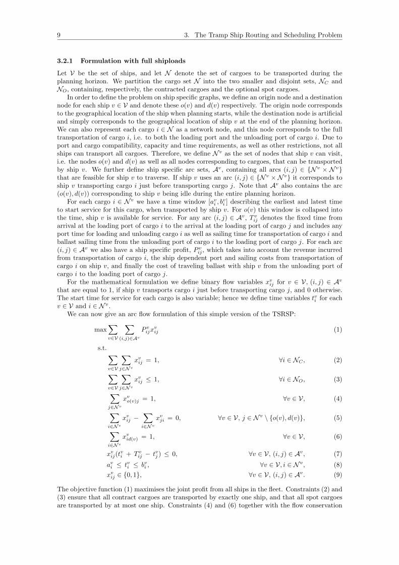
3.2.1 Formulation with full shiploads
Let V be the set of ships, and let N denote the set of cargoes to be transported during theplanning horizon. We partition the cargo set N into the two smaller and disjoint sets, NC andNO, containing, respectively, the contracted cargoes and the optional spot cargoes.
In order to define the problem on ship specific graphs, we define an origin node and a destinationnode for each ship v ∈ V and denote these o(v) and d(v) respectively. The origin node correspondsto the geographical location of the ship when planning starts, while the destination node is artificialand simply corresponds to the geographical location of ship v at the end of the planning horizon.We can also represent each cargo i ∈ N as a network node, and this node corresponds to the fulltransportation of cargo i, i.e. to both the loading port and the unloading port of cargo i. Due toport and cargo compatibility, capacity and time requirements, as well as other restrictions, not allships can transport all cargoes. Therefore, we define N v as the set of nodes that ship v can visit,i.e. the nodes o(v) and d(v) as well as all nodes corresponding to cargoes, that can be transportedby ship v. We further define ship specific arc sets, Av, containing all arcs (i, j) ∈ {N v × N v}that are feasible for ship v to traverse. If ship v uses an arc (i, j) ∈ {N v ×N v} it corresponds toship v transporting cargo i just before transporting cargo j. Note that Av also contains the arc(o(v), d(v)) corresponding to ship v being idle during the entire planning horizon.
For each cargo i ∈ N v we have a time window [avi , bvi ] describing the earliest and latest time
to start service for this cargo, when transported by ship v. For o(v) this window is collapsed intothe time, ship v is available for service. For any arc (i, j) ∈ Av, T v
ij denotes the fixed time fromarrival at the loading port of cargo i to the arrival at the loading port of cargo j and includes anyport time for loading and unloading cargo i as well as sailing time for transportation of cargo i andballast sailing time from the unloading port of cargo i to the loading port of cargo j. For each arc(i, j) ∈ Av we also have a ship specific profit, P v
ij , which takes into account the revenue incurredfrom transportation of cargo i, the ship dependent port and sailing costs from transportation ofcargo i on ship v, and finally the cost of traveling ballast with ship v from the unloading port ofcargo i to the loading port of cargo j.
For the mathematical formulation we define binary flow variables xvij for v ∈ V, (i, j) ∈ Av
that are equal to 1, if ship v transports cargo i just before transporting cargo j, and 0 otherwise.The start time for service for each cargo is also variable; hence we define time variables tvi for eachv ∈ V and i ∈ N v.
We can now give an arc flow formulation of this simple version of the TSRSP:
max∑v∈V
∑(i,j)∈Av
P vijx
vij (1)
s.t.∑v∈V
∑j∈Nv
xvij = 1, ∀i ∈ NC , (2)
∑v∈V
∑j∈Nv
xvij ≤ 1, ∀i ∈ NO, (3)
∑j∈Nv
xvo(v)j = 1, ∀v ∈ V, (4)
∑i∈Nv
xvij −∑i∈Nv
xvji = 0, ∀v ∈ V, j ∈ N v \ {o(v), d(v)}, (5)∑i∈Nv
xvid(v) = 1, ∀v ∈ V, (6)
xvij(tvi + T v
ij − tvj ) ≤ 0, ∀v ∈ V, (i, j) ∈ Av, (7)
avi ≤ tvi ≤ bvi , ∀v ∈ V, i ∈ N v, (8)
xvij ∈ {0, 1}, ∀v ∈ V, (i, j) ∈ Av. (9)
The objective function (1) maximises the joint profit from all ships in the fleet. Constraints (2) and(3) ensure that all contract cargoes are transported by exactly one ship, and that all spot cargoesare transported by at most one ship. Constraints (4) and (6) together with the flow conservation
10 3. The Tramp Ship Routing and Scheduling Problem
constraints in (5) ensure that each ship is assigned a schedule starting at the origin node andending at the destination node. Constraints (7) ensure that if ship v transports cargo i directlybefore cargo j, the time for start of service for cargo j cannot begin before service start time forcargo i plus port and travel time for transportation of cargo i plus ballast travel time with ship vfrom the unloading port of cargo i to the loading port of cargo j. Since waiting time is allowed,the constraints have an inequality sign. In constraints (8), the service start time for ship v forcargo i, tvi , is forced to be within its time window, thereby also ensuring that no ship can start itsschedule before it is available for service. Note that if ship v does not transport cargo i, the timevariable tvi has no effect and is in some sense artificial. Finally, the flow variables are restricted tobe binary in (9).
We note that constraints (7) are nonlinear and should in fact be:
xvij = 1 ⇒ tvi + T vij ≤ tvj ∀v ∈ V, (i, j) ∈ Av. (10)
However, as long as we require the xvij variables to be binary, we can easily linearise these constraintsby following the approach presented in Desrosiers et al. (1995). This approach introduces a largeconstant Mv
ij for each ship v ∈ V and each arc (i, j) ∈ Av. This constant, Mvij , must be at least
as large as the largest value that tvi + T vij − tvj can take, i.e. Mv
ij ≥ bvi + T vij − avj . The linearised
constraints then become
tvi + T vij − tvj ≤Mv
ij(1− xvij), ∀v ∈ V, (i, j) ∈ Av.
Thereby, the arc flow formulation (1)-(9) can easily be linearised. However, this is only relevant ifwe want to solve the arc flow formulation by use of standard commercial optimisation software formixed integer linear programming, and for most real life sized instances, this approach will be tootime consuming.
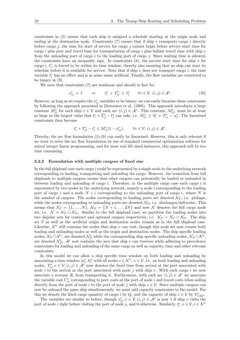
3.2.2 Formulation with multiple cargoes of fixed size
In the full shipload case each cargo i could be represented by a single node in the underlying networkcorresponding to loading, transporting and unloading the cargo. However, the transition from fullshiploads to multiple cargoes means that other cargoes can potentially be loaded or unloaded inbetween loading and unloading of cargo i. Therefore, in the multiple cargo case each cargo i isrepresented by two nodes in the underlying network, namely a node i corresponding to the loadingport of cargo i and a node N + i corresponding to the unloading port of cargo i, where N isthe number of cargoes. The nodes corresponding to loading ports are denoted NP , i.e. pickups,while the nodes corresponding to unloading ports are denoted ND, i.e. discharges/deliveries. Thismeans that NP = {1, . . . , N}, ND = {N + 1, . . . , 2N} and now N denotes the full cargo nodeset, i.e. N = NP ∪ ND. Similar to the full shipload case, we partition the loading nodes intotwo disjoint sets for contract and optional cargoes respectively, i.e. NP = NC ∪ NO. The shipset V as well as the artificial origin and destination nodes remain as in the full shipload case.Likewise, N v still contains the nodes that ship v can visit, though this node set now counts bothloading and unloading nodes as well as the origin and destination nodes. The ship specific loadingnodes, NP ∩N v, are denoted N v
P while the corresponding ship specific unloading nodes, ND ∩N v,are denoted N v
D. Av now contains the arcs that ship v can traverse while adhering to precedenceconstraints for loading and unloading of the same cargo as well as capacity, time and other relevantconstraints.
In this model we can allow a ship specific time window on both loading and unloading byassociating a time window [avi , b
vi ] with all nodes i ∈ N v, v ∈ V, i.e. on both loading and unloading
nodes. T vij , v ∈ V, (i, j) ∈ Av now denotes the fixed time from arrival at the port associated with
node i to the arrival at the port associated with node j with ship v. With each cargo i we nowassociate a revenue Ri from transporting it. Furthermore, with each arc (i, j) ∈ Av we associatethe variable cost Cv
ij corresponding to port costs at the port of node i and travel costs when sailingdirectly from the port of node i to the port of node j with ship v ∈ V. Since multiple cargoes cannow be onboard the same ship simultaneously, we must add capacity constraints to the model. Forthis we denote the fixed cargo quantity of cargo i by Qi and the capacity of ship v ∈ V by V v
CAP.The variables are similar to before, though xvij , v ∈ V, (i, j) ∈ Av is now 1 if ship v visits the
port of node i right before visiting the port of node j, and 0 otherwise. Similarly, tvi , v ∈ V, i ∈ N v
11 3. The Tramp Ship Routing and Scheduling Problem
denotes the start time for service at the port associated with node i. To keep track of the totalload onboard each ship we use variables lvi , v ∈ V, i ∈ N v \ {d(v)} which denote the total loadonboard ship v just after completing service at node i. We assume that the ship is empty whenplanning starts.
We can now present the arc flow formulation for the TSRSP with multiple cargoes of fixed sizeand no spot vessels.
max∑v∈V
∑i∈Nv
P
Rixvij −
∑v∈V
∑(i,j)∈Av
Cvijx
vij (11)
s.t.∑v∈V
∑j∈Nv
xvij = 1, ∀i ∈ NC , (12)
∑v∈V
∑j∈Nv
xvij ≤ 1, ∀i ∈ NO, (13)
∑j∈Nv
P∪{d(v)}
xvo(v)j = 1, ∀v ∈ V, (14)
∑i∈Nv
xvij −∑i∈Nv
xvji = 0, ∀v ∈ V, j ∈ N v \ {o(v), d(v)}, (15)∑i∈Nv
D∪{o(v)}
xvid(v) = 1, ∀v ∈ V, (16)
xvij(tvi + T v
ij − tvj ) ≤ 0, ∀v ∈ V, (i, j) ∈ Av, (17)
avi ≤ tvi ≤ bvi , ∀v ∈ V, i ∈ N v, (18)
xvij(lvi + Qj − lvj ) = 0, ∀v ∈ V, (i, j) ∈ Av | j ∈ N v
P , (19)
xvi,N+j(lvi − Qj − lvN+j) = 0, ∀v ∈ V, (i,N + j) ∈ Av | j ∈ N v
P , (20)
lvo(v) = 0, ∀v ∈ V, (21)∑j∈Nv
Qixvij ≤ lvi ≤
∑j∈Nv
V vCAPx
vij , ∀v ∈ V, i ∈ N v
P , (22)
0 ≤ lvN+i ≤∑j∈Nv
(V vCAP − Qi)x
vN+i,j , ∀v ∈ V, i ∈ N v
P , (23)
tvi + T vi,N+i − tvN+i ≤ 0, ∀v ∈ V, i ∈ N v
P , (24)∑j∈Nv
xvij −∑j∈Nv
xvj,N+i = 0, ∀v ∈ V, i ∈ N vP , (25)
xvij ∈ {0, 1}, ∀v ∈ V, (i, j) ∈ Av. (26)
The objective function (11) again maximises the joint profit from all ships in the fleet whileconstraints (12) and (13) ensure that all contract cargoes are transported by exactly one ship, andthat all spot cargoes are transported by at most one ship. Constraints (14) and (16) together withthe flow conservation constraints in (15) still ensure that each ship is assigned a schedule startingat the origin node and ending at the destination node, though now it is required that the firsttask in a schedule is a pickup while the last task must be a discharge. Constraints (17) ensurethat if ship v visits node i directly before node j, the time for start of service at the port of nodej cannot begin before service start time at the port of node i plus port time at the port of nodei plus travel time from the port of node i to the port of node j with ship v. Again, we have aninequality sign since waiting time is allowed. In constraints (18), the service start time for shipv at the port of node i, tvi , is forced to be within its time window, thereby also ensuring thatno ship can start its schedule before it is available for service. Note that now we also have timewindows on ports corresponding to unloading. Similar to before, if ship v does not transport cargoi, the time variables tvi and tvi+N have no effect. Constraints (19) ensure the correct relationshipbetween the binary flow variables and the ship load at each of the loading ports while constraints(20) do the same for the unloading ports. As mentioned, we assume that the ship is empty whenplanning starts and this is captured in constraints (21). The feasible interval for the ship load at
12 3. The Tramp Ship Routing and Scheduling Problem
each loading port is given by constraints (22) while constraints (23) give the same for the unloadingports. Constraints (24) ensure that a cargo cannot be unloaded before it has been loaded, andtogether with the coupling constraints (25) they ensure that the same ship performs both tasks.Note that constraints (23) can actually be omitted from the formulation due to constraints (22),(24) and (25). Finally, in constraints (26) the flow variables are, as before, restricted to be binary.
The nonlinear constraints (17), (19) and (20) can be linearised as described for the full shiploadformulation. However, we again note that for most real life sized instances this is not relevant sincethe use of standard commercial optimisation software to solve the full formulation will be too timeconsuming.
3.2.3 Allowing the use of spot vessels
If it as allowed to charter in outside spot vessels to transport some of the contract cargoes, theabove formulations can easily be modified to take this into account. For these modifications we letP si denote the profit obtained from transporting cargo i ∈ NC with a spot vessel. Note that this
profit may very well be negative. Also, we introduce binary variables si, i ∈ NC that are equal to1 if cargo i is transported by a spot vessel, and equal to 0 otherwise.
In the full shipload formulation from Section 3.2.1 the objective function (1) and constraints(2) must be modified to the following:
max∑v∈V
∑(i,j)∈Av
P vijx
vij +
∑i∈NC
P si si (27)
s.t.∑v∈V
∑j∈Nv
xvij + si = 1, ∀i ∈ NC , (28)
si ∈ {0, 1}, ∀i ∈ NC . (29)
The objective function (27) still maximises profit, though now for both the fixed fleet and for thespot vessels used. Constraints (28) ensure that each contract cargo is transported by either a shipin the fixed fleet or by a spot vessel. Finally, constraints (29) enforce binary restrictions on thespot vessel variables.
In the formulation with multiple cargoes from Section 3.2.2 the objective function (11) andconstraints (12) must similarly be modified to the following:
max∑v∈V
∑i∈Nv
P
Rixvij −
∑v∈V
∑(i,j)∈Av
Cvijx
vij +
∑i∈NC
P si si (30)
s.t.∑v∈V
∑j∈Nv
xvij + si = 1, ∀i ∈ NC , (31)
si ∈ {0, 1}, ∀i ∈ NC . (32)
3.3 Ship Routing vs. Vehicle Routing
As can be noticed from the problem description in Section 3.1 and seen from the mathematicalformulations in Section 3.2, the TSRSP is closely related to the Vehicle Routing Problem (VRP)and its many variants for which we refer the reader to Toth and Vigo (2002). Looking throughliterature, it is also quite clear that modelling approaches as well as solution methods for thesetwo problems share great similarities, and that researchers within each of the two transportationmodes have benefited from research within the other transportation mode. Literature also showsthat research on the TSRSP has lagged far behind that of the VRP, though recent years have seen ahuge increase in the amount of literature on the TSRSP. Therefore, the exchange of research ideashas most likely been far from equally balanced between the two research communities. However,we note that one of the most successful solution methods from the vehicle routing literature isbased on decomposition and dynamic column generation, and the application of this method for a
13 4. Status and Perspectives of the TSRSP
pickup and delivery problem with time windows was first studied by Appelgren (1969) for a trampship routing and scheduling application.
Even though the TSRSP is closely related to the VRP and its many variants, there are howeverimportant differences that facilitate the development of industry specific solution methods. Ronen(1983, 2002) elaborate on the operational differences between ships and trucks while Christiansenet al. (2004) add to this list of differences as well as reflect on similarities and differences betweenships and trains, and ships and aircrafts. Rather than repeating it here, we refer the reader toRonen (1983, 2002) and Christiansen et al. (2004) for an extensive discussion on the differencesbetween maritime routing and scheduling problems, and those of other transportation modes.Below we list a few of these differences including one specific for the tramp shipping industry.
• Continuous operation: As opposed to trucks, ships operate around the clock. This meansthat ship schedules usually do not have periods of idleness to absorb any delays. It also meansthat ships do not only have different starting positions but also different starting times, assome ships can be occupied with prior tasks when planning begins.
• No common depot: Even in multi-depot versions of the VRP, vehicles must return to theirhome depot, whereas ships do not have to return to their starting point.
• Compatibility issues: In shipping, compatibility issues can arise between ships and car-goes, ships and ports, and ships and canals due to equipment, capacity, draft, size etc. Eventhe flag of the ship can prevent it from entering ports in countries that have political or cul-tural issues with the nation corresponding to the flag of the ship. Even more complicating,the draft of the ship is affected by the current load of the ship, and since this affects itscompatibility with both ports and canals, the compatibility between ship and cargoes, portsand canals can be affected by the current onboard cargo.
• Optional cargoes: Specific for the TSRSP, the distinction between contract cargoes andoptional spot cargoes leads to a priority on cargoes not used in standard vehicle routingproblems where all customers must be serviced at minimum cost. In contrast, the trampobjective is to maximize profit as in the less known Pickup and Delivery Selection Problem,see Schonberger et al. (2003).
4 Status and Perspectives of the TSRSP
In this section we first review the current status of the TSRSP in Section 4.1, and afterwards discussa direction for current and future research within the area in Section 4.2. Finally, in Section 4.3we present some literature consistent with and relevant for this research direction.
4.1 Current Status of the TSRSP
As noted in Section 2, recent years have shown a dramatic increase in the amount of researchnot just within maritime transportation in general but also specifically within tramp ship routingand scheduling. Complemented by the simultaneous improvements in both software and hardware,this has made the development of both heuristic and exact methods reach a level of efficiency thatrenders many realistic sized instances of the TSRSP now solvable within reasonable time.
Even so, many tramp operators still use experienced planners to manually route and scheduletheir fleets despite the increased need for planning aid from increased fleet sizes. It is thereforeonly natural to reflect on the reasons for this. Below we list some of the reasons we believe areresponsible for this remaining gap between research and implementation.
• Conservative industry: The shipping industry has a long and proud tradition of usingplanners with practical experience from a background in shipping rather than a more aca-demic background. Therefore, most planners are very skeptical towards optimisation-basedtools not to mention reluctant to facilitate development of systems that could eventuallymake the company less dependent on them. Fagerholt (2004) presents some experience fromthe development and implementation of a decision support system for vessel fleet scheduling,
14 4. Status and Perspectives of the TSRSP
and also describes the struggle to convince the planners of the value of such a system. Atthe same time, the conservative nature of the industry has made many shipping companiesunwilling to share data for research projects, and without real life data, the gap betweenresearch and implementation naturally remains.
• Industry under pressure: Previously the research and technology were not at an ade-quate level to facilitate implementation of optimisation-based tools, and now that they areadequate, the industry is under such pressure that it is hard to find resources for anythingthat is not immediately income generating. Certainly, it can be hard to justify the allocationof resources to a research project that might in the future turn out to be valuable, whenthe company is at the same time struggling to create revenues matching just their minimumoperating costs.
• Inability to plan ahead: Uncertainty is known to play a big part in maritime optimisationwhere planners face a constantly changing environment with large daily variations in demandand many unforseen events caused, among other things, by changing weather conditions. Thisuncertainty coupled with the long voyages spanning several days and sometimes even weeks,makes it hard to plan far ahead. The financial impact, not to mention loss of goodwill, fromnot adhering to agreed cargo transportation is simply too big to allow planning far ahead.For some operators the uncertainty is so high that they cannot plan even a single voyageahead. Instead they simply wait for a ship to become idle and then assign it the currentlybest transportation request. This can for instance be the case in transportation of refined oilproducts where the unloading port and date can be unknown right up until actual unloading.A loaded ship can simply wait at sea until oil prices in ports reach a satisfactory level. Thiscan make the combinatorial puzzle, of finding the best match of ships to cargoes, seem simpleand make it even harder for conservative planners to see the potential in optimisation-basedtools.
• Dynamic nature of problem: The fact, that the basic TSRSP can be solved, is naturally arequirement for the development of planning tools in this area. However, the basic TSRSP isa static and simplified version of reality. As already mentioned, there is great uncertainty inmaritime transportation; hence, it can be necessary to continuously solve a modified versionof the problem. This means that the fleet information must continuously be updated as wellas cargo information. Note that even things such as the changing tidal conditions can affectthe solution to the problem and create cause for reoptimisation. Similarly, the planning toolmust somehow be linked to information from the spot market and continuously update thesedata. Overall, this means that the optimisation component itself will in many cases be justa very small part of the full planning tool and hence, implementation will lag behind that ofresearch within methods for solving the TSRSP.
• Modelling issues: Most mathematical models are simplified versions of reality, but inshipping this is even more so. Aside from operational considerations completely ignored inthe modelling process, those considerations that have been included in the models have beengreatly simplified. In shipping there are a lot of constraints that are simply so difficult, if notimpossible, to accurately model that simplification is the only option. To give a few exampleswe note that time windows are in reality often soft since extensions can be negotiated at acertain cost. However, this is not always possible; hence, modelling time windows as soft isnot accurate either. Similarly, the constraints describing ship-port compatibility are affectedby both the current load of the ship and the tidal conditions, and these constraints can evenin some cases be of a rather subjective nature since a risk-willing captain can agree to sail aship into a shallow port even if the draft of the ship should not allow this.
• Simplified problem: Adding to the above, the basic TSRSP is a simplified version of reality.In most cases, the problem must be extended to incorporate operator specific complexitiesin order for the solutions to be applicable in real life. Conversely, planners must find waysto modify solutions from the simplified problem in order to take into account the additionalreal-world aspects and complexities ignored in the simplified problem.
15 4. Status and Perspectives of the TSRSP
4.2 Current and Future Research Direction for the TSRSP
The first two items, and to some extent also the third, on the above list do not as such suggestfurther research within tramp ship routing and scheduling, but rather that researchers take on amore consultant like role in order to better sell their ideas to the industry. At the same time itis probably a matter of giving the shipping industry a little more time to get to a point wherethey are both interested in and able to accept optimisation-based tools. In fact, the shippingindustry has started to change in this direction by gradually employing more planners with moreacademic background and less practical experience. The third item on the list also require changesfrom within the industry itself. Operators will be able to plan further ahead if they are given moreflexibility to cope with the high uncertainty, e.g. send a different ship than originally agreed, arrivelater or earlier than planned etc.
The fourth and fifth item on the list focus mainly on the implementation side. They advocatethe development of decision support tools that have access to all necessary and continuously up-dated data, and which allow much interaction between the user and the planning tool to facilitatethe construction of several good solutions as opposed to just one solution that is, at least on paper,optimal. The development of decision support tools is certainly interesting and relevant work.However, actual implementation is not a very generic process as it will no doubt rely on the ITsystems currently used by the considered ship operator as well as other corporate characteristics.In this paper we will therefore not go further into details with the implementation side of theTSRSP though we both acknowledge and advocate for relevant work on implementation.
The last item on the above list advocates further research in the direction of development ofnew mathematical models and solution methods for tramp ship routing and scheduling. However,this research should focus on extensions of the basic problem described in Section 3 and we notethat solution methods and technology are now advanced enough to facilitate the incorporationof additional real-world complexities. The ability to solve such extended TSRSPs will hopefullyalso facilitate more implementations since the corresponding extended models will fit the realityof a broader range of tramp operators. Furthermore, even operators previously able to benefitfrom solution methods for the basic TSRSP can benefit from these extensions as they can createnew opportunities for profit maximisation as well as increased customer satisfaction. To givean example, we note that the basic TSRSP assumes that each ship sails at fixed speed whiledetermination of the actual speed along each voyage leg is left for operational planning. Recentyears have, however, shown quite a bit of research where the variable speed aspect is incorporatedinto the basic TSRSP and, not surprisingly, results show that operators can increase profits fromsuch an approach, see e.g. Norstad et al. (2011). Below is a quote from Fagerholt and Ronen(2013) supporting the general idea of further research within extensions of the basic TSRSP:
”This demonstrates that it is much more important to model and solve the right problem,considering the opportunities that often arise in practical problems, than to strive for optimal
solutions to simplified versions of the problem.”
In general, the development of research within tramp ship routing and scheduling over recent yearsis also consistent with the notion of extending the basic TSRSP to include additional complexities.In Section 4.3 we aim at scoping the basic TSRSP and present examples from literature coveringa broad range of extensions of this basic TSRSP.
4.3 Scoping the Basic TSRSP and its Extensions
Naturally, there will be quite different perceptions of what constitutes the ‘basic TSRSP’ and whatqualifies as ‘additional complexities’. Here, we let the existing literature on tramp ship routingand scheduling guide our definition of the basic problem. We do this by first noting that, althoughthe multiple cargo case is much more complex than the full shipload case, plenty of literaturedeal with multiple cargoes. We already mentioned several examples in Section 2, and adding tothis we note that, among many others, Norstad et al. (2011) also manage to incorporate furthercomplexities in the multiple cargo problem as they in this paper allow variable speed. Therefore,although the multiple cargo case does add complexity compared to the full shipload case, in ourdefinition of the ‘basic TSRSP’ we allow for both full shiploads and multiple cargoes. However, as
16 4. Status and Perspectives of the TSRSP
we noted in Section 2, flexible cargo sizes are neglected in most work on the TSRSP. This standsin contrast to the fact that flexible cargo sizes are relevant for most tramp operators transportingbulk products, and in particular liquid products. Therefore, we consider this problem characteristicas an ‘additional complexity’. Similarly, we noted in Section 2 that the multiple (non-mixable)product case is rarely considered in the existing literature on the TSRSP; hence, we do not considerthis problem characteristic as part of the basic TSRSP. Finally, we noted in Section 2 that theinclusion of spot vessels does not as such complicate the solution procedure, and that this problemcharacteristic is included in a wide variety of papers on the TSRSP. Accordingly, in our definitionof the basic TSRSP we allow the use of spot vessels, though they are certainly not required to beused.
Any complicating problem characteristic not already mentioned or implicitly excluded by themathematical formulations of the problem in Section 3.2 (e.g. variable speed), can, in our opinion,be considered an ‘additional complexity’. Thereby, the mathematical formulations presented inSections 3.2.1, 3.2.2 and 3.2.3 actually cover our definition of the basic TSRSP. Below we list someexamples of such additional complexities as well as literature on these examples.
We have already mentioned both flexible cargo sizes and multiple (non-mixable) products asadditional complexities and provided examples of work on these topics in Section 3. Again, we notethat when routing and scheduling fleets that sail full shiploads, the flexible cargo size assumptioncan be implicitly included during preprocessing.
As mentioned, an extension of the basic TSRSP, which has received a lot of attention inrecent years, is the incorporation of variable speed. This recent interest in speed optimisationhas been motivated by both steep bunker fuel price increases as well as an increased focus on theenvironmental impact of maritime transportation (and transportation in general). Examples ofrouting and scheduling combined with speed optimisation can be found in Norstad et al. (2011),Gatica and Miranda (2011) and Magirou et al. (2015).
Another topic that has recently received increased attention due to the increase in fuel prices, isthe aspect of bunkering, i.e. refueling. The main attention on this topic has been directed towardsliner shipping, see e.g. Plum et al. (2015) who present an overview of formulations, solutionmethods as well as results on this topic. In the majority of work on bunkering, the problem issolved for a fixed route, and this assumption is certainly obvious within liner shipping. However,since tramp ships do not sail according to fixed route networks, for tramp operators it seemsnatural to incorporate bunker planning in the routing and scheduling phase and this is done inVilhelmsen et al. (2014b) and Meng et al. (2015).
Recent years have also shown an increase in literature involving several parts of the supplychain. The majority of this work is related to industrial shipping, where the supply chain aspectfits naturally, since the industrial ship operator is also the cargo owner; hence, he/she is alsoresponsible for any inventory management at the ends of the maritime transportation legs. Suchsituations leads to a specific class of problems called maritime inventory routing problems. Werefer the reader to Christiansen et al. (2013) for a thorough introduction as well as literaturereview on such problems and to Andersson et al. (2010) for a comprehensive literature reviewas well as a description of the industrial aspects of combined inventory management and routingin both maritime and road-based transportation. The inventory aspect is less obvious withintramp shipping. Even so, we note that Stalhane et al. (2014) and Hemmati et al. (2015), asalready mentioned, combine tramp shipping with a vendor managed inventory service. In thiswork the tramp operator has both mandatory cargoes that must be transported, optional cargoesthat can be transported, as well as inventory pairs that may be serviced a number of times tokeep inventories within their limits. Also mentioned previously, Norstad et al. (2015) add voyageseparation requirements to the routing and scheduling problem in order to reduce inventory costsfor the charterer, and Vilhelmsen and Lusby (2014) consider basically the same problem.
Although we can find other examples of additional complexities added to the basic TSRSP, weend this section by one last example, namely the split load case, where each cargo can be splitamong several ships. This extension is considered in Korsvik et al. (2011), Stalhane et al. (2012)and Andersson et al. (2011a).
17 5. Solution Methods for the TSRSP
5 Solution Methods for the TSRSP
Most work on the TSRSP and its extensions contains a problem specific arc flow formulation or referto similar work, that contains such a formulation. Most of these formulations can, just as the onespresented in Section 3.2, easily be linearised, and, in theory, solved by use of standard commercialoptimisation software for mixed integer linear programming. An example of this approach can befound in Norstad et al. (2015). However, as already mentioned in Section 3.2, and also concluded inNorstad et al. (2015), for most real life sized instances, this approach will be too time consuming.In this section we therefore discuss some methods and tools commonly used to solve the TSRSPand extensions of it. We also relate these methods and tools to literature within the area.
As can be seen from Section 2, the methods used to solve the TSRSP and its extensions are quitediverse, ranging from simple heuristics to exact methods. Naturally, the choice of method mustdepend on the complexity of the problem at hand as well as requirements for solution quality andcomputation time. Even though literature contains a broad range of both problems and methods,one method seems to receive much more attention than any of the others: Column generation. Wetherefore dedicate Section 5.1 to a generic description of the exact column generation approachfor the TSRSP. Section 5.2, on the other hand, focuses on heuristic solution approaches for theTSRSP.
5.1 Column Generation
The popularity of column generation is in line with research within many other fields. We note thatboth crew scheduling and vehicle routing problems are very often solved using this approach, andthat the method has achieved great success within these areas and many others, see e.g. Butcherset al. (2001) and Toth and Vigo (2002). Furthermore, Desaulniers et al. (2005) devoted two wholechapters to column generation in maritime problems. Looking through the literature, it seemsthat this approach has become more popular within recent years where focus has been on TSRSPextensions. This is on one hand a little surprising since the added complexity contained in theseextensions should indicate the use of heuristic methods to achieve reasonable running times. Onthe other hand, the increase in software and hardware has allowed more focus on exact methods,and one of the main advantages of the column generation approach is that it allows complicatingconstraints to be handled in ship specific subproblems which generate the columns. Furthermore,it should be noted that even though this is an exact method, it can easily be modified in a heuristicdirection as we discuss in Section 5.2.1. No matter the heuristic or exact nature of the method,the frequent use of the column generation approach for a broad range of complex instances, notjust within shipping but also within many other research areas, demonstrates the great advantageand flexibility of this method that allows easy incorporation of complicating constraints.
5.1.1 Master Problem
Since most of the TSRSP constraints relate to a specific ship, it seems natural to decomposethe problem and use column generation. Whether we use a priori column generation or dy-namic/delayed column generation, the master problem of such a decomposition is the same. Itis a path formulation containing only the constraints which couple the ships together and ensurethat each ship follows exactly one path. In the basic TSRSP, the coupling constraints correspondto constraints (2) and (3), or equivalently (12) and (13), though these must be expressed by newpath flow variables while a similar reformulation of the original objective function (1) or (11) mustbe performed.
To arrive at this new path formulation for the basic TSRSP as well as many of its extensions,we let Rv denote the set of all feasible schedules for ship v. We denote the profit of a schedule bypvr for r ∈ Rv and define a binary schedule variable λvr that is equal to 1 if ship v sails schedule r,and 0 otherwise. The profit pvr is calculated based on information from the underlying schedule,which holds all necessary information, i.e. the ship it is constructed for, the cargoes carried, andthe timing of port calls during the schedule. Finally, we let the parameter avir be equal to 1 if shipv carries cargo i in schedule r, and 0 otherwise. As earlier, N denotes the set of cargoes to betransported and can be partitioned into NC and NO containing, respectively, the set of contractcargoes and the set of optional cargoes.
18 5. Solution Methods for the TSRSP
The master problem is now given by the following path flow reformulation of the original arcflow model:
max∑v∈V
∑r∈Rv
pvrλvr (33)
s.t.∑v∈V
∑r∈Rv
avirλvr = 1, ∀i ∈ NC , (34)∑
v∈V
∑r∈Rv
avirλvr ≤ 1, ∀i ∈ NO, (35)∑
r∈Rv
λvr = 1, ∀v ∈ V, (36)
λvr ∈ {0, 1}, ∀v ∈ V, r ∈ Rv. (37)
The objective function (33) maximises profit from chosen schedules. Constraints (34) and (35) arethe path flow reformulations of constraints (2) and (3), respectively, or equivalently (12) and (13).The convexity constraints (36) and binary restrictions on the schedule variables in (37) ensure thateach ship is assigned exactly one schedule. Note that if the problem is to be solved by Branch-and-Bound, it is helpful to insert explicit slack variables in constraints (35). If such slack variablesare added to constraints (35), we recognise the master problem as a Set Partitioning Problem inwhich the columns correspond to feasible ship schedules.
For the TSRSP, and most of its extensions, there is no need to include all feasible schedulesfor each ship in the master problem. Instead we can limit the column set to contain the profitmaximising schedule for each combination of ship and cargo set. There can, however, be situationswhere additional coupling constraints in the master problem means that the profit maximisingschedule for one ship and cargo set is not necessarily profit maximising when taking the entirefleet into account. This is the case in Vilhelmsen and Lusby (2014) where they have temporaldependencies between the schedules for different ships. These dependencies require the enumerationof all feasible schedules rather than just all profit maximising schedules.
Accordingly, two schedules in the master problem might correspond to the same route butdiffer in other aspects, e.g. the timing of port calls. For some applications, non-integer solutionsto the master problem can be considered feasible as long as the (fractionally) selected schedulesfor a specific ship all correspond to the same geographical route. Constraints (36) ensure thatthe schedule for each ship is a convex combination of different schedules for the same ship whileconstraints (37) must be rewritten to ensure that the schedules included in the convex combinationcorrespond to the same geographical route. This means that the binary restrictions in (37) can bereplaced by restrictions of the form
{r : λvr > 0} correspond to equal geographical routes, ∀v ∈ V. (38)
If convex schedule combinations are used, a greater part of the solution space can be spannedwithout generating as many columns as would be required if not utilising such convex combina-tions. This approach is used in e.g. Christiansen and Nygreen (1998) for a ship routing problemwith inventory constraints and Vilhelmsen and Lusby (2014) also allow such convex schedule com-binations. However, there can be many situations where convex schedule combinations do notqualify as actual schedules, primarily due to cost calculations. One example is when the TSRSP isextended to allow variable speed as in Norstad et al. (2011). Since the fuel consumption function isa convex function of speed, once we include variable speed we can no longer allow convex schedulecombinations, since the convex combination of schedule costs would overestimate the actual costof the schedule. Therefore, we must select exactly one schedule for each ship. Another example isin the work presented in Vilhelmsen et al. (2014b) where the TSRSP is extended to include bunkerplanning. In this case the schedules also contain information on bunker stops, and each of thesestops corresponds to a predefined price for a specific bunker option at a given time. Assume nowthat two schedules for the same ship each contain a stop at a bunker option, B, though at differ-ent times denoted tB1 and tB2 with different bunker prices, PB
1 and PB2 , respectively. The convex
combination of these two schedules will have an arrival time somewhere in the interval (tB1 , tB2 ),
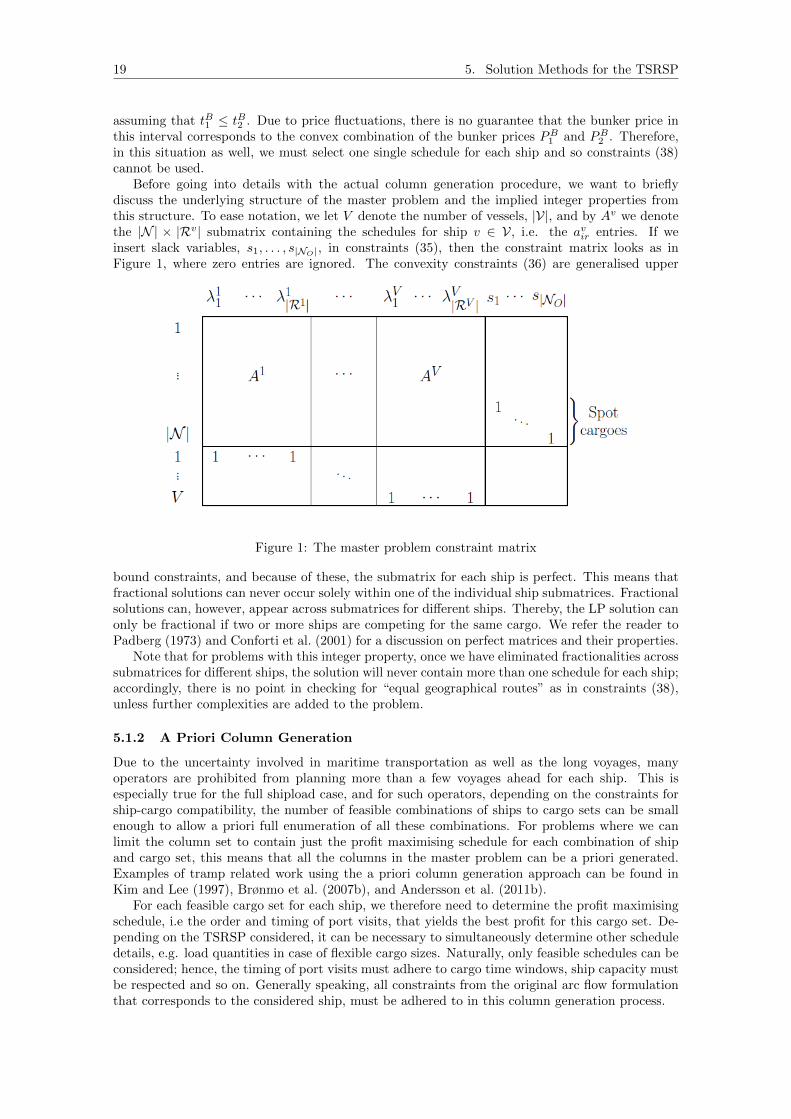
19 5. Solution Methods for the TSRSP
assuming that tB1 ≤ tB2 . Due to price fluctuations, there is no guarantee that the bunker price inthis interval corresponds to the convex combination of the bunker prices PB
1 and PB2 . Therefore,
in this situation as well, we must select one single schedule for each ship and so constraints (38)cannot be used.
Before going into details with the actual column generation procedure, we want to brieflydiscuss the underlying structure of the master problem and the implied integer properties fromthis structure. To ease notation, we let V denote the number of vessels, |V|, and by Av we denotethe |N | × |Rv| submatrix containing the schedules for ship v ∈ V, i.e. the avir entries. If weinsert slack variables, s1, . . . , s|NO|, in constraints (35), then the constraint matrix looks as inFigure 1, where zero entries are ignored. The convexity constraints (36) are generalised upper
Figure 1: The master problem constraint matrix
bound constraints, and because of these, the submatrix for each ship is perfect. This means thatfractional solutions can never occur solely within one of the individual ship submatrices. Fractionalsolutions can, however, appear across submatrices for different ships. Thereby, the LP solution canonly be fractional if two or more ships are competing for the same cargo. We refer the reader toPadberg (1973) and Conforti et al. (2001) for a discussion on perfect matrices and their properties.
Note that for problems with this integer property, once we have eliminated fractionalities acrosssubmatrices for different ships, the solution will never contain more than one schedule for each ship;accordingly, there is no point in checking for “equal geographical routes” as in constraints (38),unless further complexities are added to the problem.
5.1.2 A Priori Column Generation
Due to the uncertainty involved in maritime transportation as well as the long voyages, manyoperators are prohibited from planning more than a few voyages ahead for each ship. This isespecially true for the full shipload case, and for such operators, depending on the constraints forship-cargo compatibility, the number of feasible combinations of ships to cargo sets can be smallenough to allow a priori full enumeration of all these combinations. For problems where we canlimit the column set to contain just the profit maximising schedule for each combination of shipand cargo set, this means that all the columns in the master problem can be a priori generated.Examples of tramp related work using the a priori column generation approach can be found inKim and Lee (1997), Brønmo et al. (2007b), and Andersson et al. (2011b).
For each feasible cargo set for each ship, we therefore need to determine the profit maximisingschedule, i.e the order and timing of port visits, that yields the best profit for this cargo set. De-pending on the TSRSP considered, it can be necessary to simultaneously determine other scheduledetails, e.g. load quantities in case of flexible cargo sizes. Naturally, only feasible schedules can beconsidered; hence, the timing of port visits must adhere to cargo time windows, ship capacity mustbe respected and so on. Generally speaking, all constraints from the original arc flow formulationthat corresponds to the considered ship, must be adhered to in this column generation process.
20 5. Solution Methods for the TSRSP
The column generation in the a priori approach therefore consists of repeatedly determiningthe optimal route and schedule for a given ship and a given cargo set. This can be done e.g. bysimply enumerating all feasible routes for the given cargo set or by dynamic programming. Someinstances of the TSRSP and its extensions will, however, be too large to allow full enumerationof all combinations of ships to cargo sets. In such cases it is possible to instead use dynamiccolumn generation as described below. The enumeration approach is used in e.g. Brønmo et al.(2007b) while the dynamic programming approach, on the other hand, is used in e.g. Fagerholtand Christiansen (2000b).
5.1.3 Dynamic Column Generation
As already mentioned, some instances of the TSRSP and its extensions will be too large to allow fullenumeration of all combinations of ships to cargo sets, and some situations require the enumerationof all feasible schedules rather than just all profit maximising schedules. Therefore, for severalreasons, there can be situations where the a priori column generation approach is prohibited. Insuch situations, dynamic column generation can be used, and this is the approach used in e.g.Stalhane et al. (2012), Vilhelmsen et al. (2014b) and Coccola et al. (2015). We refer the reader toDesaulniers et al. (2005) for a detailed description of this method.
We also note that both Appelgren (1969) and Brønmo et al. (2010) have found dynamic columngeneration more efficient than a priori generation for situations where a priori generation wasactually possible. They find the dynamic approach both faster and more flexible as it allows themto deal with larger and more loosely constrained instances than the a priori approach.
In the dynamic column generation approach, the master problem initially only contains a smallsubset, R′v, of the feasible schedules for each ship v ∈ V, and new columns that have the potentialto improve the current master problem solution are then generated iteratively. The new columnsare generated in subproblems, or pricing problems, derived from a Dantzig-Wolfe decomposition,and there are as many independent subproblems as there are ships. Each subproblem correspondsto a specific ship and contains all constraints related to this ship from the original formulation. Ineach iteration we solve the restricted master problem (RMP), which is the linear relaxation of theoriginal master problem though with only its current restricted column set. The dual variablesfrom this solution are then used to guide the generation of promising columns in the subproblems,which are added to the master problem, whereafter a new iteration begins. This process continuesuntil no further promising columns can be generated. At that point, the current solution to theRMP is optimal for the linear relaxation of the original master problem with all feasible schedulesin the column set.
The purpose of the subproblems is to generate ship specific schedules that can potentiallyimprove the current solution to the RMP. This in turn corresponds to finding feasible scheduleswith positive reduced costs in the current RMP solution. Since only feasible schedules should begenerated, the subproblem must contain all relevant constraints for the corresponding ship, e.g.time windows and capacity constraints.
To illustrate the structure of these subproblems, we let σi be the dual variables for constraints(34) and (35). The variables corresponding to (34) are free of sign while the variables correspondingto (35) must be nonnegative. Furthermore, we let ωv be the dual for constraint (36) which is alsofree of sign. Finally, we define πi = σi for all i ∈ N and πo(v) = ωv corresponding to the originnode. If we first restrict our attention to the simple full shipload TSRSP formulation presented inSection 3.2.1, the corresponding subproblem for ship v is given by:
max∑
(i,j)∈Av
(P vij − πi
)xvij (39)
s.t.
(4)− (9). (40)
The objective function (39) maximises the reduced cost with respect to the current dual variables,and the constraints (4)-(9) ensure that only feasible schedules are considered. If the optimalschedule has a positive reduced cost, it has the potential to improve the current RMP; hence, itwill be represented by a new column in the RMP.
21 5. Solution Methods for the TSRSP
For the multiple cargo formulation from Section 3.2.2, the subproblem for ship v is given by:
max∑i∈Nv
P
Rixvij −
∑(i,j)∈Av
(Cv
ij + πi)xvij (41)
s.t.
(14)− (26). (42)
The objective function (41) again maximises the reduced cost with respect to the current dualvariables, and the constraints (14)-(26) again ensure that only feasible schedules are considered.
Each subproblem can be modelled as an elementary shortest path problem with time win-dows (ESPPTW). The ESPPTW has been proven NP-hard in the strong sense by Dror (1994);hence, no pseudo-polynomial algorithms are likely to exist for this problem. When more complexTSRSPs are considered, the subproblems are most often more general elementary shortest pathproblems with resource constraints (ESPPRC) which are also NP-hard in the strong sense sincethey generalise the ESPPTW. This is for instance the situation for the multiple cargo case, where,in addition to time, ship capacity is also a constraining resource. The ESPPRC, and thereby alsothe ESPPTW, entails finding an elementary shortest path between two nodes while satisfying theresource constraints, e.g. time windows and capacity constraints.
In maritime transportation, and in particular within deep sea shipping, voyages travel timesare often so long that few, if any, time feasible cycles can be expected in the subproblem networks.Therefore, it is quite common to relax the subproblem to allow non elementary paths, since the reg-ular shortest path problem with resource constraints (SPPRC) can be solved in pseudo polynomialtime (see e.g. Desrochers and Soumis (1988); Irnich and Desaulniers (2005)). This relaxation isused in e.g. Brønmo et al. (2010) and Vilhelmsen et al. (2014b). Note though that if time-feasiblecycles do in fact exist, schedules can be generated where the same cargo is transported more thanonce. In such cases, the solution method must be modified to handle these cycles.
The SPPRC is typically solved by dynamic programming algorithms on the underlying shipspecific networks, and this is also the approach used in both Brønmo et al. (2010) and Vilhelmsenet al. (2014b). We refer the reader to Desaulniers et al. (1998), Irnich and Desaulniers (2005)and Irnich (2008) for a thorough introduction to the SPPRC, the related dynamic programmingalgorithms, and several associated concepts.
5.1.4 The Column Generation Scheme
When a priori column generation has been applied, the number of columns in the master problem isoften sufficiently small to allow the master problem to be solved directly by commercial optimisationsoftware for mixed integer programs and thereby obtain an optimal integral solution. This approachis used in e.g. Fagerholt and Christiansen (2000b) and Fagerholt (2001). When the column countbecomes too large for this approach, we must instead solve the linear relaxation of the masterproblem, and then apply a Branch-and-Bound procedure if the optimal solution is fractional.
When columns have been generated dynamically, once the column generation phase is com-pleted, we have an optimal solution to the linear relaxation of the original master problem in (33)-(37). If this solution is fractional, the column generation procedure must also be embedded in aBranch-and-Bound framework where new columns are generated in each node of the search tree.In this case, the entire procedure is called a Branch-and-Price procedure, since new columns arepriced out in each node of the tree.
The strong integer property of the constraint matrix means that the linear relaxation of themaster problem will provide very tight upper bounds. This property is verified in Vilhelmsen et al.(2014b), where they incorporate bunker planning in the TSRSP. There, they experience relativelyfew fractional solutions, and for those fractional solutions they do encounter, the IP gap is verysmall. Note however that when extending the basic TSRSP, the additional complexities addedto the basic model can easily compromise the strong integer property of the constraint matrix.Examples of this can be found in the work on split loads by Stalhane et al. (2012), on vendormanaged inventory by Stalhane et al. (2014) and on voyage separation requirements by Vilhelmsenand Lusby (2014). In each of these cases, the considered extension creates an interdependencebetween schedules for different ships such that these new constraints must remain in the masterproblem rather than being added to the subproblems.
22 5. Solution Methods for the TSRSP
5.1.5 Branching
When in fact branching is required, the branching scheme is very often tailor made to the specificapplication considered. However, one generic method that seems to be frequently used for trampshipping, as well as other scheduling problem such as e.g. crew scheduling and vehicle routingproblems, is that of constraint branching, and we discuss this approach below. Since constraintbranching is not a complete branching strategy, this approach must often be complemented byother branching schemes. Another generic branching approach used within tramp shipping as wellas other areas, is that of time window branching which we also discuss below.
Constraint branching was introduced by Ryan and Foster (1981), and is an efficient branchingscheme developed for solving set partitioning and set packing problems. Within tramp shipping,this branching approach exploits the underlying structure of the constraint matrix by noting thatwithin any optimal fractional solution, there must be a cargo i ∈ N that is transported (fraction-ally) by several ships. Since, by definition, each spot vessel (slack variables can also be viewed as aform of spot vessel schedules) can only transport one cargo, the spot vessels cannot compete witheach other for cargoes. Therefore, at least one of the ships currently competing for cargo i mustbe a non-spot vessel and we denote this ship k. For each ship v ∈ V and cargo i ∈ N we introducethe sum
Svi =
∑r∈R′v
avirλvr .
If the current solution is fractional, there must exist a cargo i and a regular ship k ∈ V for which0 < Sk
i < 1. In an integral solution, the cargo can only be transported by one ship and so ship kcan either transport or not transport cargo i. The branching strategy is therefore to construct a1-branch where ship k is forced to transport cargo i and a 0-branch where ship k is not allowed totransport cargo i. In the 1-branch this means that akir = 1 should hold for all r ∈ R′k. Thereby,we can remove all schedules for ship k that do not include cargo i and all schedules for other shipsthat do include cargo i, either explicitly or implicitly by simply setting their upper bounds equalto zero. This also means removing any spot vessel schedule for cargo i. Furthermore, we removecargo i in all subproblem networks not corresponding to ship k. Without further modifications itis possible for the subproblem of ship k to construct new schedules that do not include cargo i.Different ways of overcoming this problem exist, the simplest of which simply relies on the dualvariables to eventually enforce the construction of schedules for ship k that include cargo i. In the0-branch, we instead have akir = 0 for all r ∈ R′k. This is the opposite process of the 1-branch, andso we instead remove all schedules for k that do include cargo i. Furthermore, we remove cargoi in the subproblem network corresponding to ship k while we cannot make any changes in thenetworks corresponding to other ships.
To ease notation, we let SSi denote the similar sum for spot vessels (including slack variables).
When 0 < SSi < 1, we can then use the same branching approach as just described for regular
ships though the corresponding updates of the RMP and subproblems must of course be modifiedaccordingly.
Competition for a cargo i requires at least two different ships. Thereby, in a fractional solutionthere must be at least two distinct ships (one of them possibly a spot vessel), k1 and k2, for whichSk1i and Sk2
i are fractional. Therefore, in any fractional solution we have at least two candidatecargo-ship pairs for branching and we must select one of these. The approach for selecting thebranching pair varies in the literature as basically two different opinions on this selection exist:
Most integer: Select the vessel cargo pair with largest Ski . In other words, from the set of all
candidate pairs C, where
C = {(i, k) ∈ NC ∪NO × V ∪ {S} : 0 < Ski < 1},
we select
(i, k)∗ = arg max(i,k)∈C
{Ski
}.
23 5. Solution Methods for the TSRSP
The premise is that a value close to 1 is evidence to suggest that ship k most likely transportscargo i in an optimal integer solution. If the largest Sk
i is, however, much smaller than 1, itseems more intuitive to enforce a 0-branch by picking pair (i′, k′) with the smallest Sk
i . Asmall value of Sk
i indicates that the ship is unlikely to transport cargo i. One typically sets athreshold value for the largest Sk
i , e.g. 0.8, prior to solving the problem. If the largest valueis at least the threshold, a 1-branch is enforced, while a 0-branch is enforced otherwise.
Most fractional: If Ski is close to 1, the solution favours ship k for transporting cargo i; hence,
forcing ship k to transport the cargo, as we do in the 1-branch, might not change the solutionmuch and thereby not the upper bound either. In the 0-branch, where we force ship k not totransport the cargo, we can on the other hand expect to see a greater impact on the upperbound. This could potentially create an unbalanced search tree. The situation is similar,though reversed, if Sk
i is close to 0. To maintain a balanced search tree we might thereforeprefer branching on candidates that are as fractional as possible, i.e. as close to 1/2. In suchcases we would hence select the following candidate pair to branch on:
(i, k)∗ = arg min(i,k)∈C
{∣∣Ski −
1
2
∣∣}.Examples of work on the TSRSP using constraint branching can be found in Stalhane et al. (2012)and Vilhelmsen and Lusby (2014).
Time window branching was originally presented by Gelinas et al. (1995) as a branching schemeto restore integrality. As mentioned in Section 5.1.3, for some applications and solution methodsit is possible to generate cyclic schedules, i.e. schedules where the same cargo is transportedmore than once. The presence of such schedules in the master problem will compromise the stronginteger property of the constraint matrix and therefore also cause trouble for the constraint branch-ing scheme described above. In such situations time window branching complements constraintbranching very nicely, as it can be used to eliminate cycles, though the approach can be useful formuch more than just that.
The basic concept in time window branching is to split a given time window into two smallertime windows that each correspond to a new problem, i.e. to a new branch in the branch-and-bound search tree. The key to success with this branching scheme is to select a good time windowto split on, and furthermore to select a good split time for this specific time window. This splittime must be chosen in such a way that the current solution becomes infeasible in each of the twonew problems, i.e. in a way that makes at least one currently chosen schedule infeasible in eachnew branch.
We illustrate this process in Figure 2 for the time window [ai, bi] corresponding to a cargo iwhich is currently transported by two schedules, or twice in a cycle by the same schedule. Thestart times of these two visits are denoted T 1
i and T 2i , respectively. The grey boxes in Figure 2
correspond to the so called feasibility interval of each of these two visits. These intervals, [T 1i , u1]
and [T 2i , u2], contain all the start times that will allow the corresponding schedule to still remain
feasible. This will most often correspond to redistributing waiting time; hence, we have depictedthese feasibility intervals as extensions of the current visit times. Since these two intervals aredisjoint, we can choose a split time within (u1, T
2i ], say ts, and create one branch where the time
window for cargo i is [ai, ts − ε] and the second visit is infeasible, and one branch where the timewindow is [ts, bi] where the first visit is infeasible. Here, ε > 0 is a very small tolerance.Note that split times within one of the feasibility intervals would also render one visit infeasiblein each branch. However, during the next iteration of schedule generation, the visit, for which weselected a split time within its feasibility interval, could be regenerated though only a little laterin time. After branching, all previously generated schedules violating these new time windows,are removed from the master problem in each new branch and the corresponding subproblems areupdated to reflect the new time windows.
How to choose the specific time window to branch on and also what exact split time to usewithin this time window, can depend on the considered application though a generic and detailedapproach can be found in Gelinas et al. (1995). They propose three strategies for choosing whichtime window to branch on; namely focusing on elimination of important cycles, focusing on the
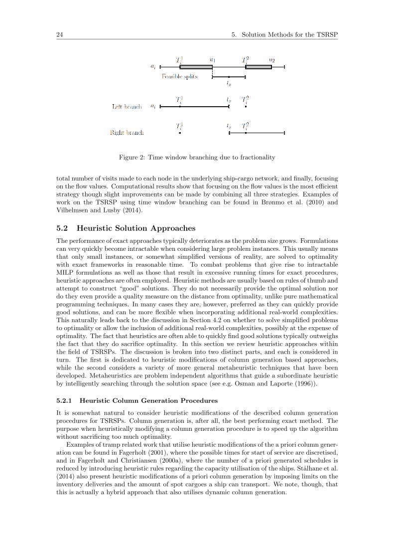
24 5. Solution Methods for the TSRSP
Figure 2: Time window branching due to fractionality
total number of visits made to each node in the underlying ship-cargo network, and finally, focusingon the flow values. Computational results show that focusing on the flow values is the most efficientstrategy though slight improvements can be made by combining all three strategies. Examples ofwork on the TSRSP using time window branching can be found in Brønmo et al. (2010) andVilhelmsen and Lusby (2014).
5.2 Heuristic Solution Approaches
The performance of exact approaches typically deteriorates as the problem size grows. Formulationscan very quickly become intractable when considering large problem instances. This usually meansthat only small instances, or somewhat simplified versions of reality, are solved to optimalitywith exact frameworks in reasonable time. To combat problems that give rise to intractableMILP formulations as well as those that result in excessive running times for exact procedures,heuristic approaches are often employed. Heuristic methods are usually based on rules of thumb andattempt to construct “good” solutions. They do not necessarily provide the optimal solution nordo they even provide a quality measure on the distance from optimality, unlike pure mathematicalprogramming techniques. In many cases they are, however, preferred as they can quickly providegood solutions, and can be more flexible when incorporating additional real-world complexities.This naturally leads back to the discussion in Section 4.2 on whether to solve simplified problemsto optimality or allow the inclusion of additional real-world complexities, possibly at the expense ofoptimality. The fact that heuristics are often able to quickly find good solutions typically outweighsthe fact that they do sacrifice optimality. In this section we review heuristic approaches withinthe field of TSRSPs. The discussion is broken into two distinct parts, and each is considered inturn. The first is dedicated to heuristic modifications of column generation based approaches,while the second considers a variety of more general metaheuristic techniques that have beendeveloped. Metaheuristics are problem independent algorithms that guide a subordinate heuristicby intelligently searching through the solution space (see e.g. Osman and Laporte (1996)).
5.2.1 Heuristic Column Generation Procedures
It is somewhat natural to consider heuristic modifications of the described column generationprocedures for TSRSPs. Column generation is, after all, the best performing exact method. Thepurpose when heuristically modifying a column generation procedure is to speed up the algorithmwithout sacrificing too much optimality.
Examples of tramp related work that utilise heuristic modifications of the a priori column gener-ation can be found in Fagerholt (2001), where the possible times for start of service are discretised,and in Fagerholt and Christiansen (2000a), where the number of a priori generated schedules isreduced by introducing heuristic rules regarding the capacity utilisation of the ships. Stalhane et al.(2014) also present heuristic modifications of a priori column generation by imposing limits on theinventory deliveries and the amount of spot cargoes a ship can transport. We note, though, thatthis is actually a hybrid approach that also utilises dynamic column generation.
25 5. Solution Methods for the TSRSP
The dynamic column generation approach can also be heuristically modified and in the literaturewe find several examples of this. In Brønmo et al. (2010), where flexible cargo sizes are allowed, theauthors use a two-stage approach for the subproblems. In this approach the otherwise continuouscargo quantity variables are discretised, since this allows them to follow a more standard dynamicprogramming algorithm for solving the subproblem. Afterwards, for the p best solutions to thediscretised subproblems, the authors find the optimal continuous load quantities for each of thesep routes by solving an LP. In Vilhelmsen et al. (2014b), where the integration of bunker planningin the TSRSP is considered, a similar approach by discretising the otherwise continuous bunkerpurchase variables is followed. Stalhane et al. (2012) also use a heuristic modification of dynamiccolumn generation as they only consider a subset of the actual arcs in their subproblem networksand limit the length of the paths generated.
5.2.2 Metaheuristics
The field of metaheuristics encompasses a wide range of algorithms, which can be used to intelli-gently search the solution space without the tractability issues of large mathematical programmingformulations. Examples of well known metaheuristics include, but are not limited to, local searchprocedures, tabu search, and genetic algorithms. They are iterative generation processes that in-telligently guide the search to promising parts of the solution space. Due to its complexity, it isnot surprising that several examples of metaheuristics can be found in the TSRSP literature.
Local search procedures consider the immediate neighbours of a potential solution in the hopeof locating and moving to an improved solution. Generally speaking, a neighbour of a givensolution is almost identical to the solution, differing in only one or two components. Startingfrom an initial solution a local search heuristic iteratively considers a neighbouring solution ofthe current solution and accepts the neighbouring solution if it yields a better objective function.Iterations are performed as long as a terminating criterion (e.g. time limit or iteration count) isnot satisfied. An application of local search within tramp ship routing and scheduling can be foundin Brønmo et al. (2007a) in which the authors propose a multi-start local search heuristic for themultiple cargo TSRSP. Rather than starting with just one initial solution, a multi-start local searchprocedure provides several initial solutions, each of which is considered for improvement, in thehope of diversifying the search. In Brønmo et al. (2007a) a set of initial solutions is obtained usinga procedure with random and deterministic elements to assign cargoes to ships. The best solutionsof these are improved using a so-called quick version of their local search, which considers threeneighbourhoods: an intra ship schedule operator, and two inter schedule operators. With the intraschedule operator, a cargo is selected and removed from the schedule it is in. The cargo is thenreinserted into the same schedule in the best possible location. The first of the two inter scheduleoperators is the same, with the exception that the removed cargo is moved to its best locationacross all other ship schedules. The second inter schedule operator is of a similar flavour wherebytwo cargoes are selected and inserted into each of the other’s schedules. Each neighbourhood isused with a certain frequency. An attempt is then made to further improve the best solutionsfrom the quick version by running an extended version of the local search. Five neigbourhoods areused in this stage. Three of these are identical to those of the quick version, while the remainingtwo are extensions of two of these. The first is an intra schedule operator that re-sequences twocargoes, while the second is an inter schedule operator where three cargoes i, j, and k, are selectedand removed from ships u, v, and w. The cargoes are then reinserted into ships v, w, and u. Theperformance of the metaheuristic is compared with that of a priori column generation approach.Computational results show that the multi-start local search procedure returns optimal or near-optimal solutions within reasonable time for real-life instances. Norstad et al. (2011) extend theframework of Brønmo et al. (2007a) to consider variable speed. The algorithm is structurally thesame; however, an additional step which optimizes the speed of the ship is conducted whenever anew ship schedule enters the solution.
Tabu search is a well known metaheuristic in Operations Research literature and was first pro-posed in Glover (1986). This is essentially an improved local search procedure, differing in twomain aspects. First, moves to previously visited solutions for a certain number of iterations areforbidden (i.e. tabooed). However, moves to neighbouring solutions with a worse objective arepermitted. Both extensions are an attempt to diversify the search. Accepting worse solutions from
26 5. Solution Methods for the TSRSP
time to time also guards against getting stuck in a local optimum. Examples of tabu search pro-cedures within tramp ship routing and scheduling can be found in Korsvik et al. (2010), Fagerholtet al. (2011), and Korsvik and Fagerholt (2010).
Korsvik et al. (2010) propose a tabu search approach for the multiple cargo problem consideredin Brønmo et al. (2007a). The authors generate an initial solution by first sorting unassignedcargoes in order of the start of the time window for the loading port. Cargoes are then sequentiallyassigned to the ship that results in minimum cost. Furthermore, the loading and unloading portsare inserted in the best positions in the ship’s partial schedule. The neighbourhood defined forthe improvement phase is quite simple and similar to the first of the two inter schedule operatorsof Brønmo et al. (2007a); the authors select a cargo, remove it from the schedule it was in andmove it to a different ship’s schedule. When a cargo is removed from a schedule it is forbiddenfrom being assigned to the ship it was removed from for a certain number of iterations. Inserting acargo into a schedule is done at minimum cost using simple insertions, i.e. the ordering of the portcalls already in the schedule remains unchanged. To improve the running times a neighbourhoodreduction technique is employed. Furthermore, moves to infeasible solutions are permitted, and thealgorithm runs for a specified number of iterations. Periodic schedule re-optimization is performedat regular intervals to re-optimize the order of the port calls within a ship schedule. The authorscompare the results of their method with those of the multi-start local search heuristic describedabove. Computational results suggest that the tabu search algorithm performs better than themulti-start local search heuristic, especially for large and tightly constrained problems. Fagerholtet al. (2011) consider project shipping with cargo stowage and cargo coupling constraints, a specialreal-life TSRSP, and propose a modified version of the tabu search algorithm in Korsvik et al.(2010) to solve the problem. The structure of the tabu search procedure is largely unchanged.Again, computational results show that the tabu search heuristic yields optimal or near-optimalsolutions within reasonable time.
Korsvik and Fagerholt (2010) present a tabu search algorithm for solving the TSRSP withflexible cargo sizes. The algorithm is very similar in structure to that of Korsvik et al. (2010).However, there are some differences. First, the authors use a randomly generated initial solution.Second, moves to infeasible solutions are not permitted. Instead, the authors introduce a secondneighbourhood for the improvement phase. The additional neighbourhood is also similar to oneof the neighbourhoods proposed in Brønmo et al. (2007a) and focuses on swapping two cargoes(from different ships) between the ships. Again, the cargoes are inserted into the ship schedulesusing simple insertion strategies, which leave the order of the previous cargoes unchanged. For agiven ship schedule a fast quantity optimization heuristic is then used to determine its optimalcargo quantities. Finally, the algorithm terminates when a set number of iterations have elapsed.Computational results show that the tabu search procedure provides optimal or near-optimalsolutions within reasonable time for real-life instances.
A slightly different variant of local search, known as Variable Neighbourhood Search (VNS),has also been proposed by Malliappi et al. (2011) for the multiple cargo TSRSP. VNS was first pro-posed by Mladenovic and Hansen (1997) and is a metaheuristic approach for solving combinatorialoptimization problems. As the name suggests, the algorithm utilises local search, but with theaddition of a perturbation phase to allow the algorithm to search distant neighbours of the incum-bent solution. Within each neighbourhood local search is applied to find a local optimum. Like allother metaheuristic approaches, VNS must be initialized with a feasible solution. For this, Malli-appi et al. (2011) consider the cargoes in non-increasing order of the quantity to be carried. Thecargoes are sequentially added to ships, being inserted in the best possible position for the firstfeasible ship. If no feasible assignment exists for a given cargo it is assigned to a dummy ship. Oncean initial solution is obtained the two level VNS algorithm is activated. The outer level determinesin which neighbourhood to randomly generate a neighbour of the incumbent solution. For this sixdifferent neighbourhoods are proposed. Three of which are based on selecting a different numberof ships and deleting δ% of the assigned cargoes on each. The other three operators re-sequencea cargo within a schedule, reassign a cargo to a different schedule, or swap two cargoes (fromdifferent ships) between the ships. The purpose of the outer level is to “shake” the solution to adistant neighbourhood. The so-called shaking neighbourhoods are considered in turn and for eachthe local search neighbourhoods of Brønmo et al. (2007a) are iteratively considered to find a localoptimum. The authors compare their method to both the tabu search heuristic of Korsvik et al.
27 5. Solution Methods for the TSRSP
(2010) and the multi-start local search method of Brønmo et al. (2007a), though with their ownimplementation of these two methods. Computational results from modified benchmark instancesfrom land transportation show that the VNS, on average, performs best.
Large Neighbourhood Search (LNS) is another well known technique in the metaheuristic field.First proposed by Shaw (1997), this procedure is an extension of the local search strategy inwhich the neighbourhood can be extremely large. Unlike, the traditional local search procedure,neighbouring solutions need not be structurally similar and can, in fact, be very different. Suchlarge neighbourhoods can assist in diversifying the search. An example of LNS in tramp shiprouting and scheduling can be found in Korsvik et al. (2011). The authors consider ship routingallowing split loads. An initial solution is constructed by randomly selecting a cargo one byone from a list of unassigned cargoes and assigning it a random ship until all cargoes have beenassigned. A simple insertion strategy, like that of Brønmo et al. (2007a), is used to find the bestplaces within the schedule for the loading and unloading ports. No split loads are consideredinitially. This initial solution is improved using a local search heuristic that considers four differentneighbourhoods. Two of these consider reassigning cargoes; one reassigns a given cargo to anothership, while the other swaps two cargoes between two different ships. The remaining two considerthe splitting/merging of cargoes. The improvement phase consists of successive iterations of aso-called destroy-and-repair algorithm. That is, at every iteration the solution is destroyed byremoving a randomly selected number of cargoes. The solution is then repaired using several fastinsertion heuristics, and subsequently optimised using the four neighbourhood local search heuristicdescribed above. Results indicate that the authors’ approach is able to provide good solutions toreal-life instances in reasonable time.
The Adaptive Large Neighbourhood Search Procedure of Ropke and Pisinger (2006) extendsthe LNS to multiple neighbourhoods. Adaptive Large Neighbourhood Search (ALNS) procedurestypically have several large neighbourhoods defined and each is assigned a weight reflecting theperformance of the neighbourhood. Over time the weights are updated to reflect the relative successof each of the neighbourhoods and essentially ensure the algorithm searches in areas where it hashad greatest success. ALNS procedures within tramp ship routing and scheduling can be foundin Hemmati et al. (2014) and Hemmati et al. (2015). Hemmati et al. (2014) apply an ALNS to abenchmark suite of tramp shipping instances and report high quality results. The algorithm startswith an initial solution in which no cargoes are assigned to ships. In the subsequent improvementphase, the algorithm chooses between three different destroy (or removal) heuristics followed bya choice of two insertion heuristics. The authors consider a random removal, where q randomlychosen cargoes are removed, the so-called Shaw removal in which q similar cargoes are removed,and a worst removal, in which the q cargoes with highest cost are removed. Regarding the insertionheuristics, a greedy insertion based heuristic as well as a regret based heuristic are used. Initiallyall destroy and repair methods are equally likely to be chosen; however, over time the selectionweights are adjusted to ensure better performing heuristics are chosen. Hemmati et al. (2015)describe an application of this ALNS procedure to solve the vendor managed inventory problemintroduced in Stalhane et al. (2014). Results indicate that the metaheuristic approach is, for themost part, competitive with an exact procedure in terms of solution quality, but superior to aheuristic column generation approach.
Finally, genetic algorithms have been used to solve a wide variety of optimisation problems.A genetic algorithm (GA) is an optimisation method for solving a wide range of problems con-strained as well as unconstrained. It is based on a natural selection process that mimics biologicalevolution. A set of individual feasible solutions are denoted a population and this population isthen modified in each of the iterations. In each iteration of the genetic algorithm it randomlyselects individuals from the current population and uses them as parents to produce the childrenfor the next generation. Applications of GAs within tramp ship routing and scheduling can befound in Lin and Liu (2011), Kang et al. (2012), and Jung et al. (2011). Lin and Liu (2011) proposea GA for the multiple cargo TSRSP. The proposed GA outperforms a mathematical formulation,which is solved directly by a commercial solver. The MILP formulation used, however, is differentto that which is used in the above references. Kang et al. (2012), and Jung et al. (2011) focus ona quite specific TSRSP involving the transportation of cars.
28 6. Concluding Remarks
6 Concluding Remarks
In this paper we have provided a thorough introduction to the general area of tramp ship routingand scheduling. We have reviewed the most recent literature on tramp ship routing and schedul-ing and provided the reader with a general understanding of the problem, as well as modelingapproaches for it. We have also provided an analysis of both the current status and the futuredirection of research within the area and provided the reader with a general knowledge on solutionmethods for tramp ship routing and scheduling problems. Thereby, this paper can be used toprovide researchers, new to the field, with a comprehensive understanding of this research topic.
We have argued that, in order for the shipping industry to fully benefit from the research alreadyconducted on the TSRSP, attention should now be given to actual implementation. We have alsoargued that one of the main directions of current and future research lies in the development ofmodels and methods for extensions of the basic TSRSP rather than in the development of newmethods for the basic problem. Such extensions will enable more tramp operators to benefitfrom the solution methods, while simultaneously creating new opportunities for operators alreadybenefitting from existing methods.
Although some TSRSP extensions, such as variable speed, are quite generic, a lot of extensionswill be operator specific. Therefore, it is hard to point in any one direction for future research withrespect to extensions. With this being said, we do however want to mention two interesting researchtopics that, in our opinion, deserve great attention in future research within tramp shipping:
• We find that the static and deterministic approach in most work on tramp shipping con-stitutes a huge simplification for most operators. In fact, uncertainty plays a big part inmaritime optimization where planners face a constantly changing environment with manyunforseen events and large daily variations in demand. Weather and currents have a hugeimpact on sailing plans but in addition to this it is quite common within tramp shippingthat the discharge port is to some extent unknown even at loading time. Furthermore, portconditions such as strikes and lack of available berths can delay loading and unloading, andnew cargoes are continuously revealed. Naturally, one must walk before one can run, butnow that the basic TSRSP can be solved efficiently, it seems obvious to expand the researchto include both dynamic and stochastic models. Adding to this the open-ended nature ofthe TSRSP, it seems only natural to embed solution methods into a rolling horizon approach(see e.g. Sethi and Sorger (1991)), e.g. as in Meng et al. (2015), and/or to incorporate avalue of time to account for the occupation of ships, e.g. as in Appelgren (1969). Boththese approaches should then incorporate any information on future demand. The dynamicand stochastic nature of the problem also calls for considerations to solution robustness andpersistence, i.e. consistency between planning and realization, so that the whole fleet is notrescheduled due to a small delay with one ship.
• As already mentioned, the work presented in Norstad et al. (2015), Vilhelmsen and Lusby(2014), Stalhane et al. (2014) and Hemmati et al. (2015) relates the TSRSP to the broadercontext of the supply chain. In industrial shipping, where the ship operator is also the cargoowner, the supply chain aspect seems obvious and much literature in this area also includesthis aspect, see Christiansen et al. (2013). Even though this aspect seems less obvious ina tramp shipping setting, it is still a very interesting topic for further research, and wesee two main reasons for this. First, in a market with tough competition and freight ratesalready critically low, it seems obvious for tramp operators to instead improve their customerservice through inventory management services in order to attract more business. Second,optimising over the entire supply chain, or at least parts of it, rather than just the isolatedTSRSP, will no doubt enable overall cost reductions. With the right collaboration setup,some part of these cost reductions will reflect back on the tramp operator and allow anincrease in profit. Furthermore, we note that including information from the supply chainwill also give a better understanding of future demand and thereby assist in resolving theissue from above regarding dynamic and stochastic modelling approaches.
29 References
Acknowledgements
The research presented in this paper has been partly funded by The Danish Maritime Fund andwe gratefully acknowledge their financial support.
References
H. Andersson, A. Hoff, M. Christiansen, G. Hasle, and A. Lokketangen. Industrial aspects andliterature survey: Combined inventory management and routing. Computers & Operations Re-search, 37(9):1515–1536, 2010.
H. Andersson, M. Christiansen, and K. Fagerholt. The maritime pickup and delivery problem withtime windows and split loads. INFOR, 49(2):79–91, 2011a.
H. Andersson, J.M. Duesund, and K. Fagerholt. Ship routing and scheduling with cargo couplingand synchronization constraints. Computers & Industrial Engineering, 61(4):1107–1116, 2011b.
L.H. Appelgren. A column generation algorithm for a ship scheduling problem. TransportationScience, 3:53–68, 1969.
L.H. Appelgren. Integer programming methods for a vessel scheduling problem. TransportationScience, 5:64–78, 1971.
G. Brønmo, M. Christiansen, K. Fagerholt, and B. Nygreen. A multi-start local search heuristic forship scheduling - a computational study. Computers & Operations Research, 34:900–917, 2007a.
G. Brønmo, M. Christiansen, and B. Nygreen. Ship routing and scheduling with flexible cargosizes. Journal of the Operational Research Society, 58(9):1167–1177, 2007b.
G. Brønmo, B. Nygreen, and J. Lysgaard. Column generation approaches to ship scheduling withflexible cargo sizes. European Journal of Operational Research, 200(1):139–150, 2010.
B.D. Brouer, J.F. Alvarez, C.E.M. Plum, D. Pisinger, and M.M. Sigurd. A base integer program-ming model and benchmark suite for liner-shipping network design. Transportation Science, 48(2):281–312, 2014.
E.R. Butchers, P.R. Day, A.P Goldie, S. Miller, J.A. Meyer, D.M. Ryan, A.C. Scott, and C.A.Wallace. Optimized crew scheduling at air new zealand. Interfaces, 31(1):30–56, 2001.
K.K. Castillo-Villar, R.G. Gonzalez-Ramırez, P.M. Gonzalez, and N.R. Smith. A heuristic proce-dure for a ship routing and scheduling problem with variable speed and discretized time windows.Mathematical Problems in Engineering, 2014.
M. Christiansen and B. Nygreen. A method for solving ship routing problems with inventoryconstraints. Annals of Operations Research, 81:357–378, 1998.
M. Christiansen, K. Fagerholt, and D. Ronen. Ship routing and scheduling: Status and perspectives(review). Transportation Science, 38(1):1–18, 2004.
M. Christiansen, K. Fagerholt, B. Nygreen, and D. Ronen. Maritime transportation. In C. Barnhartand G. Laporte, editors, Transport. Handbooks in Operations Research and Management Science,vol. 14, chapter 4, pages 189–284. Elsevier, North-Holland, Amsterdam, 2007.
M. Christiansen, K. Fagerholt, B. Nygreen, and D. Ronen. Ship routing and scheduling in the newmillennium (review). European Journal of Operational Research, 228(3):467–483, 2013.
M.E. Coccola, R. Dondo, and C.A. Mendez. A MILP-based column generation strategy for manag-ing large-scale maritime distribution problems. Computers & Chemical Engineering, 72:350–362,2015.
M. Conforti, G. Cornuejols, A. Kapoor, and K. Vuskovic. Perfect, ideal and balanced matrices.European Journal of Operational Research, 133(3):455–461, 2001.
30 References
G. Desaulniers, J. Desrosiers, I. Ioachim, M.M. Solomon, F. Soumis, and D. Villeneuve. A unifiedframework for deterministic time constrained vehicle routing and crew scheduling problems. InT. Crainic and G. Laporte, editors, Fleet Management and Logistics, chapter 3, pages 57 – 94.Kluwer Academic Publishers, 1998.
G. Desaulniers, J. Desrosiers, and M.M. Solomon, editors. Column Generation. Springer, NewYork, 2005.
M. Desrochers and F. Soumis. A reoptimization algorithm for the shortest path problem with timewindows. European Journal of Operational Research, 35:242 – 254, 1988.
J. Desrosiers, Y. Dumas, M.M. Solomon, and F. Soumis. Time constrained routing and scheduling.In M.O. Ball, T.L. Magnanti, C.L. Monma, and G.L. Nemhauser, editors, Network Routing.Handbooks in Operations Research and Management Science, vol. 8, chapter 2, pages 35–139.North-Holland, Amsterdam, 1995.
M. Dror. Note on the complexity of the shortest path models for column generation in VRPTW.Operations Research, 42(5):977–978, 1994.
K. Fagerholt. Ship scheduling with soft time windows: An optimisation based approach. EuropeanJournal of Operational Research, 131(3):559–571, 2001.
K. Fagerholt. A computer-based decision support system for vessel fleet scheduling - experienceand future research. Decision Support Systems, 37(1):35–47, 2004.
K. Fagerholt and M. Christiansen. A combined ship scheduling and allocation problem. Journalof the Operational Research Society, 51:834 – 842, 2000a.
K. Fagerholt and M. Christiansen. A travelling salesman problem with allocation, time windowand precedence constraints - an application to ship scheduling. International Transactions inOperational Research, 7(3):231 – 244, 2000b.
K. Fagerholt and D. Ronen. Bulk ship routing and scheduling: Solving practical problems mayprovide better results. Maritime Policy & Management, 40(1):48–64, 2013.
K. Fagerholt, L.M. Hvattum, T.A.V. Johnsen, and J.E. Korsvik. Routing and scheduling in projectshipping. Annals of Operations Research, pages 1–15, 2011.
R.A. Gatica and P.A. Miranda. Special issue on latin-american research: A time based discretiza-tion approach for ship routing and scheduling with variable speed. Networks and Spatial Eco-nomics, 11(3):465–485, 2011.
S. Gelinas, M. Desrochers, J. Desrosiers, and M.M. Solomon. A new branching strategy for timeconstrained routing problems with application to backhauling. Annals of Operations Research,61:91–109, 1995.
F. Glover. Future paths for integer programming and links to artificial intelligence. Computers &Operations Research, 13(5):533–549, 1986.
A. Hemmati, L.M. Hvattum, K. Fagerholt, and I. Norstad. Benchmark suite for industrial andtramp ship routing and scheduling problems. INFOR, 52(1):28–38, 2014.
A. Hemmati, M. Stalhane, L.M. Hvattum, and H. Andersson. An effective heuristic for solvinga combined cargo and inventory routing problem in tramp shipping. Computers & OperationsResearch, 64:274 – 282, 2015.
ICS. International Chamber of Shipping Website (accessed 14.08.2015),http://www.ics-shipping.org/shipping-facts/shipping-and-world-trade.
S. Irnich. Resource extension functions: properties, inversion, and generalization to segments. ORSpectrum, 30(1):113–148, 2008.
31 References
S. Irnich and G. Desaulniers. Shortest path problems with resource constraints. In G. Desaulniers,J. Desrosiers, and M.M. Solomon, editors, Column Generation, chapter 2, pages 33 – 66. Springer,2005.
J.N. Jung, M.N. Kang, H.R. Choi, H.S. Kim, B.J. Park, and C.H. Park. Development of a geneticalgorithm for the maritime transportation planning of car carriers. Dynamics in logistics, 6:481–488, 2011.
M.H. Kang, H.R. Choi, H.S. Kim, and B.J. Park. Development of a maritime transportationplanning support system for car carriers based on genetic algorithm. Applied Intelligence, 36(3):585–604, 2012.
S.-H. Kim and K.-K. Lee. An optimization-based decision support system for ship scheduling.Computers & Industrial Engineering, 33(3-4):689–692, 1997.
K. Kobayashi and M. Kubo. Optimization of oil tanker schedules by decomposition, column gener-ation, and time-space network techniques. Japan Journal of Industrial and Applied Mathematics,27(1):161–173, 2010.
J.E. Korsvik and K. Fagerholt. A tabu search heuristic for ship routing and scheduling with flexiblecargo quantities. Journal of Heuristics, 16(2):117–137, 2010.
J.E. Korsvik, K. Fagerholt, and G. Laporte. A tabu search heuristic for ship routing and scheduling.Journal of the Operational Research Society, 61(4):594–603, 2010.
J.E. Korsvik, K. Fagerholt, and G. Laporte. A large neighbourhood search heuristic for ship routingand scheduling with split loads. Computers & Operations Research, 38(2):474–483, 2011.
S.A. Lawrence. International Sea Transport: The Years Ahead, pages 1–316. Lexington Books,Lexington, MA., 1972.
D.-Y. Lin and H.-Y. Liu. Combined ship allocation, routing and freight assignment in trampshipping. Transportation Research Part E: Logistics and Transportation Review, 47(4):414–431,2011.
E.F. Magirou, H.N. Psaraftis, and T. Bouritas. The economic speed of an oceangoing vessel in adynamic setting. Transportation Research Part B: Methodological, 76:48–67, 2015.
F. Malliappi, J.A. Bennell, and C.N. Potts. A variable neighborhood search heuristic for tramp shipscheduling. Lecture Notes in Computer Science (including subseries Lecture Notes in ArtificialIntelligence and Lecture Notes in Bioinformatics), 6971 LNCS:273–285, 2011.
Q. Meng, S. Wang, and C.-Y. Lee. A tailored branch-and-price approach for a joint tramp shiprouting and bunkering problem. Transportation Research Part B: Methodological, 72:1 – 19,2015.
N. Mladenovic and P. Hansen. Variable neighborhood search. Computers & Operations Research,24(11):1097–1100, 1997.
K.-H. Neo, H.-C. Oh, and I.A. Karimi. Routing and cargo allocation planning of a parcel tanker.In 16th European Symposium on Computer Aided Process Engineering and 9th InternationalSymposium on Process Systems Engineering, pages 1985 – 1990, 2006.
I. Norstad, K. Fagerholt, and G. Laporte. Tramp ship routing and scheduling with speed opti-mization. Transportation Research Part C: Emerging Technologies, 19(5):853–865, 2011.
I. Norstad, K. Fagerholt, L.M. Hvattum, H.S. Arnulf, and A. Bjørkli. Maritime fleet deploymentwith voyage separation requirements. Flexible Services and Manufacturing Journal, 27(2-3):180–199, 2015.
32 References
H.-C. Oh and I.A. Karimi. Routing and scheduling of parcel tankers: a novel solution approach.In A. Bruzzone, F. Longo, Y. Merkuriev, G. Mirabello, and M.A. Piera, editors, The 11thInternational Workshop on Harbor Maritime Multimodal Logistics Modeling and Simulation,pages 98 – 103, September 2008.
I. H. Osman and G Laporte. Metaheuristics: A bibliography. Annals of Operations Research, 63:513–623, 1996.
M. Padberg. On the facial structure of set packing polyhedra. Mathematical Programming, 5(1):199–215, 1973.
D.J. Papageorgiou, G.L. Nemhauser, J. Sokol, M.-S. Cheon, and A.B. Keha. MIRPLib - A libraryof maritime inventory routing problem instances: Survey, core model, and benchmark results.European Journal of Operational Research, 235(2):350 – 366, 2014.
C.E.M. Plum, D. Pisinger, and P.N. Jensen. Bunker purchasing in liner shipping. In Chung-YeeLee and Qiang Meng, editors, Handbook of Ocean Container Transport Logistics, InternationalSeries in Operations Research and Management Science, pages 251–278. Springer, 2015.
D. Ronen. Cargo ships routing and scheduling: Survey of models and problems. European Journalof Operational Research, 12(2):119–126, 1983.
D. Ronen. Ship scheduling: The last decade. European Journal of Operational Research, 71(3):325–333, 1993.
D. Ronen. Marine inventory routing: Shipments planning. Journal of the Operational ResearchSociety, 53(1):108–114, 2002.
S. Ropke and D. Pisinger. An adaptive large neighborhood search heuristic for the pickup anddelivery problem with time windows. TRANSPORTATION SCIENCE, 40(4):455–472, 2006.
D.M. Ryan and B. Foster. An integer programming approach to scheduling. Computer Scheduling ofPublic Transport. Urban Passenger Vehicle and Crew Scheduling. Proceedings of an InternationalWorkshop, pages 269–280, 1981.
J. Schonberger, H. Kopfer, and D.C. Mattfeld. A combined approach to solve the pickup anddelivery selection problem. In U. Leopold-Wildburger, F. Rendl, and G. Wascher, editors,Operations Research Proceedings 2002, pages 150–155. Springer, 2003. Selected Papers of theInternational Conference on Operations Research (SOR 2002), Klagenfurt, September 2-5, 2002.
S. Sethi and G. Sorger. A theory of rolling horizon decision making. Annals of Operations Research,29:387–416, 1991.
P. Shaw. A new local search algorithm providing high quality solutions to vehicle routing problems,1997.
M. Stalhane, H. Andersson, M. Christiansen, J.-F. Cordeau, and G. Desaulniers. A branch-price-and-cut method for a ship routing and scheduling problem with split loads. Computers &Operations Research, 39(12):3361–3375, 2012.
M. Stalhane, H. Andersson, M. Christiansen, and K. Fagerholt. Vendor managed inventory intramp shipping. Omega (United Kingdom), 47:60–72, 2014.
P. Toth and D. Vigo. The vehicle routing problem. SIAM, 2002.
UNCTAD. Review of maritime transport 2013. http://unctad.org/en/PublicationsLibrary/rmt2013en.pdf, 2013.
UNCTAD. Review of maritime transport 2014. http://unctad.org/en/PublicationsLibrary/rmt2014en.pdf, 2014.
33 References
C. Vilhelmsen and R.M. Lusby. Tramp ship routing and scheduling with voyage separation re-quirements. Technical Report, Department of Management Engineering, Technical University ofDenmark, 2014.
C. Vilhelmsen, J. Larsen, and R.M. Lusby. A heuristic and hybrid method for the tank allocationproblem in maritime bulk shipping. Technical Report, Department of Management Engineering,Technical University of Denmark, 2014a.
C. Vilhelmsen, R.M. Lusby, and J. Larsen. Tramp ship routing and scheduling with integratedbunker optimization. Euro Journal of Transportation and Logistics, 3(2):143–175, 2014b.