training for ecdl advanced spreadsheetstraining for ecdl advanced spreadsheets a practical course in...
TRANSCRIPT
Training for ECDL
Advanced Spreadsheets
A Practical Course in Windows XP and Office 2007
Lorna Bointon
Blackrock Education Centre, 2010

© Blackrock Education CentreISBN 978-0-9564074-0-5
Published byBlackrock Education Centre, Kill Avenue, Dún Laoghaire, Co. Dublin, Ireland.
Tel. (+353 1) 2 302 709 Fax. (+353 1) 2 365 044E-mail: [email protected] www.becpublishing.com and www.blackrockec.ie
First published, 2010
All rights reserved. No part of this publication may be reproduced, stored in a retrieval system or transmitted, in any form or by any means without the prior written permission of the publisher, nor be otherwise circulated in any form of binding or cover other than that in which it is published and without a similar condition being imposed on any subsequent purchaser or user.
Microsoft® Windows®, Microsoft® Office, Microsoft Word, Microsoft Access, Microsoft Excel, Microsoft PowerPoint®, Microsoft Internet Explorer and Microsoft Outlook® are either registered trademarks or trademarks of the Microsoft Corporation.
Other products mentioned in this manual may be registered trademarks or trademarks of their respective companies or corporations.
The companies, organisations, products, the related people, their positions, names, addresses and other details used for instructional purposes in this manual and its related support materials on the manual’s support website www.becpublishing.com are fictitious. No association with any real company, organisations, products or people are intended nor should any be inferred.

Contents
Note to Reader ....................................................................................................................................v
CHAPTER 1 Formatting ..............................................................................................................................................1
CHAPTER 2 Functions and Formulas ........................................................................................................... 25
CHAPTER 3 Charts ....................................................................................................................................................... 69
CHAPTER 4 Analysis .................................................................................................................................................. 93
CHAPTER 5 Validating and Auditing ........................................................................................................ 161
CHAPTER 6 Enhancing Productivity ......................................................................................................... 191
CHAPTER 7 Collaborative Editing ............................................................................................................... 229
Checklist ............................................................................................................................................ 249
Index ..................................................................................................................................................... 255

Note to Reader
The ManualAdvanced Spreadsheets for Microsoft Office 2007 for ECDL offers a practical, step-by-step guide for those who wish to upgrade their spreadsheet skills to acquire a thorough competence in this application. Similar to the other Blackrock Education Centre training materials, it has been designed as either a stand-alone study guide or for use in a tutor-led environment. However, as is characteristic of Blackrock Education Centre training materials, the content of this manual offers additional support information through explanations, demonstrations and practical exercises as well as a support website, www.becpublishing.com.
DesignEvery use has been made of the expertise we have gained training students in ICT over many years. The knowledge and skills of our substantial pool of trainers hugely influenced the content and layout of the material.
The manual is written in plain English.•
There are step-by-step, detailed explanations and action sequences. •
Particular attention is given to relating what is seen on the pages of the manual to what is seen •on the computer screen.
The A4 size of the manual and the side-by-side layout of graphics and text, combine to make it •an ideal training manual.
ExercisesAt the end of each section, there are two kinds of exercises. There are self-check questions designed to jog your memory of important details. There are also practical exercises that have been designed to revise some of the more important skills associated with using Microsoft Excel.
In successfully completing each set of exercises, the student can be confident, that progress in learning more sophisticated skills has been achieved.
Web SupportSupport material is available on the CD enclosed in the manual and on the internet at www.becpublishing.com.
This manual was produced – text, design and layout – using only the Microsoft Office suite of programs and the skills described in the manual. The screen shots were captured using
a small utility program and most were inserted directly onto the page.
1
Formatting Chapter 1 Training for ECDL
10 Unauthorised Photocopying is Unlawful
1.2.3 Applying Customised Cell Styles Select the cell or range of cells to be formatted with the new style. From the Home tab and the Styles group, select the Cell Styles arrow.
The new style will be displayed in the Custom section of the drop-down menu. Select the custom style to apply it to the selected cell(s).
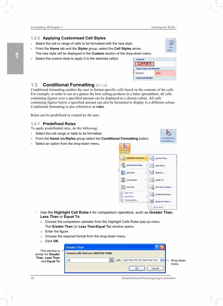
1.3 Conditional Formatting (4.1.1.2) Conditional formatting enables the user to format specific cells based on the contents of the cells. For example, in order to see at a glance the best selling products in a Sales spreadsheet, all cells containing figures over a specified amount can be displayed in a chosen colour. All cells containing figures below a specified amount can also be formatted to display in a different colour. Conditional formatting is also referred to as rules. Rules can be predefined or created by the user. 1.3.1 Predefined Rules To apply predefinded rules, do the following: Select the cell range or table to be formatted. From the Home tab/Styles group select the Conditional Formatting button. Select an option from the drop-down menu.
Use the Highlight Cell Rules for comparison operators, such as Greater Than, Less Than or Equal To. o Choose the comparison operator from the Highlight Cells Rules pop-up menu.
The Greater Than (or Less Than/Equal To) window opens. o Enter the figure. o Choose the required format from the drop-down menu. o Click OK.
o o o
This window issimilar for GreaterThan, Less Than
and Equal To Drop-down menu
Training for ECDL Chapter 1 Formatting
Unauthorised Photocopying is Unlawful 11
Use the Highlight Cell Rules Between comparison operator to find cell content between a specified highest and lowest figure. o Choose Between from the Highlight Cells Rules pop-up menu. The Between window opens. o Enter the highest and lowest figures. o Choose the required format from the drop-down menu. o Click OK.
Use the Highlight Cell Rules Text that Contains option to format cells that contain specified text.. o Choose Text that Contains from the Highlight Cells Rules pop-up menu. The Text That Contains window opens. o Enter the text that will be formatted when used. o Choose the required format from the drop-down menu. o Click OK.
Use the Highlight Cell Rules A Date Occurring option to format cells containing a specified date. o Choose A Date Occurring from the Highlight Cells Rules pop-up menu. The A Date Occurring window opens. o Enter the date that will be formatted when it is used. o Choose the required format from the drop-down menu. o Click OK.
Enter the highest and
lowest figures
Choose a format for cell content between the specified figures to be displayed in
Enter the text
Choose a format for the specified text
Select a date
Choose a format for the specified date

1
Formatting Chapter 1 Training for ECDL
10 Unauthorised Photocopying is Unlawful
1.2.3 Applying Customised Cell Styles Select the cell or range of cells to be formatted with the new style. From the Home tab and the Styles group, select the Cell Styles arrow.
The new style will be displayed in the Custom section of the drop-down menu. Select the custom style to apply it to the selected cell(s).
1.3 Conditional Formatting (4.1.1.2) Conditional formatting enables the user to format specific cells based on the contents of the cells. For example, in order to see at a glance the best selling products in a Sales spreadsheet, all cells containing figures over a specified amount can be displayed in a chosen colour. All cells containing figures below a specified amount can also be formatted to display in a different colour. Conditional formatting is also referred to as rules. Rules can be predefined or created by the user. 1.3.1 Predefined Rules To apply predefinded rules, do the following: Select the cell range or table to be formatted. From the Home tab/Styles group select the Conditional Formatting button. Select an option from the drop-down menu.
Use the Highlight Cell Rules for comparison operators, such as Greater Than, Less Than or Equal To. o Choose the comparison operator from the Highlight Cells Rules pop-up menu.
The Greater Than (or Less Than/Equal To) window opens. o Enter the figure. o Choose the required format from the drop-down menu. o Click OK.
o o o
This window issimilar for GreaterThan, Less Than
and Equal To Drop-down menu
Training for ECDL Chapter 1 Formatting
Unauthorised Photocopying is Unlawful 11
Use the Highlight Cell Rules Between comparison operator to find cell content between a specified highest and lowest figure. o Choose Between from the Highlight Cells Rules pop-up menu. The Between window opens. o Enter the highest and lowest figures. o Choose the required format from the drop-down menu. o Click OK.
Use the Highlight Cell Rules Text that Contains option to format cells that contain specified text.. o Choose Text that Contains from the Highlight Cells Rules pop-up menu. The Text That Contains window opens. o Enter the text that will be formatted when used. o Choose the required format from the drop-down menu. o Click OK.
Use the Highlight Cell Rules A Date Occurring option to format cells containing a specified date. o Choose A Date Occurring from the Highlight Cells Rules pop-up menu. The A Date Occurring window opens. o Enter the date that will be formatted when it is used. o Choose the required format from the drop-down menu. o Click OK.
Enter the highest and
lowest figures
Choose a format for cell content between the specified figures to be displayed in
Enter the text
Choose a format for the specified text
Select a date
Choose a format for the specified date

1
Formatting Chapter 1 Training for ECDL
12 Unauthorised Photocopying is Unlawful
Use the Highlight Cell Rules Duplicate Values option to format cells that contain duplicate or unique values. o Choose Duplicate Values from the Highlight Cells Rules pop-up menu. The Duplicate window opens. o Choose Duplicate or Unique (if only occurring once) o Choose the required format from the drop-down menu. o Click OK.
Use Top/Bottom Rules to format cells with the Top or Bottom items; Top or Bottom 10% or Above or Below average.
o Choose Top 10 Items (or Top 10%, etc.) from the Top/Bottom Rules pop-up menu. The Top 10 Items (or Top 10%, etc.) window opens. o Choose the number of cells that will rank in the top (or bottom). o Choose the required format from the drop-down menu. o Click OK.
Select Duplicate or
Unique
Choose a format for duplicate values
Choose a format Choose the
number of cells that rank in the
Top (or Bottom)
Training for ECDL Chapter 1 Formatting
Unauthorised Photocopying is Unlawful 13
Use the Data Bars option to colour data in a cell.
o Choose Data Bars. o Choose the required colour from the menu. Using Data Bars, the longer the colour bar, the higher the value in the cell.
Use the Color Scales option to display colours from the red, green, blue and yellow
colour scales to display as gradient colours where each colour indicates a value.
o Choose Color Scales. o Choose the required colour from the pop-up menu. Using Colour Scales, the lowest figure may display in red and the highest value in green, with the remainder of the cells displaying in yellow.
Use the Icon Sets option to display an icon representing a value in each cell. The icon displays next to the figure in the cell. o Choose Icon Sets. o Choose the required icon set from the pop-up menu.
Using Icon Sets, figures can be displayed with a red cross for low values and a green tick for the highest values.
Lowest figure displayed in red
Highest figure displayed in green
Lowest figuresdisplayed with red X Highest figures displayed with green
Choose an icon to present the selected values
2
Functions and Formulas Chapter 2 Training for ECDL
34 Unauthorised Photocopying is Unlawful
1.2 Mathematical Functions (4.2.1.2) Mathematical functions can be entered directly into a cell or inserted from the Function Library. The latter method displays the Function Arguments window, facilitating the process by prompting the user to enter values within specific boxes. Mathematical functions include Rounding figures up or down, and using Sum functions, such as SumIf. 1.2.1 Rounddown The Round function is used to round figures up or down (towards or away from zero). The Rounddown function rounds a number down towards zero (0). To use the rounddown function, do the following: Click into the cell in which the Rounddown function is to be inserted and displayed. Select the Formulas tab. From the Function Library group, select the Math & Trig arrow. Scroll down the list and select Rounddown.
The Function Arguments window opens.
Enter the cell reference which contains the number or enter the number that you want to round down.
Enter the number of digits in the Num_digits box to which the figure should be rounded. Select OK.
1.2.2 Roundup The Round function is used to round figures up or down (towards or away from zero). Roundup rounds figures up away from zero (0) to a specified number of digits. To use the roundup function, do the following: Click into the cell in which the Roundup function is to be inserted and displayed. Select the Formulas tab. From the Function Library group, select the Math & Trig arrow. Scroll down the list and select Roundup.
The Function Arguments window opens.
Training for ECDL Chapter 2 Functions and Formulas
Unauthorised Photocopying is Unlawful 35
The Rounddown and Roundup functions can also be entered manually.
Select the cell in which the function is to be entered and displayed. Enter the = sign. Enter the function ROUNDDOWN to round a figure down towards zero or
ROUNDUP to round a figure up, away from zero. As you enter the function name a menu appears. Double-click an option or do the following:
Enter an open round bracket (. Enter the cell, e.g. =ROUNDDOWN(A1 or =ROUNDUP(A1. Enter a comma followed by the number of digits that you want to round down or
up, e.g. =ROUNDDOWN(A1, 0 or =ROUNDUP(A1, 0. Close the bracket, e.g. =ROUNDDOWN(A1, 0) or =ROUNDUP(A1, 0).
Alternatively, after the open bracket, drag the mouse over the cell range to select it and press Enter.
Enter the cell reference which contains the number or enter the number that you want to round up.
Enter the number of digits in the Num_digits box to which the figure should be rounded (up, away from zero).
Select OK.
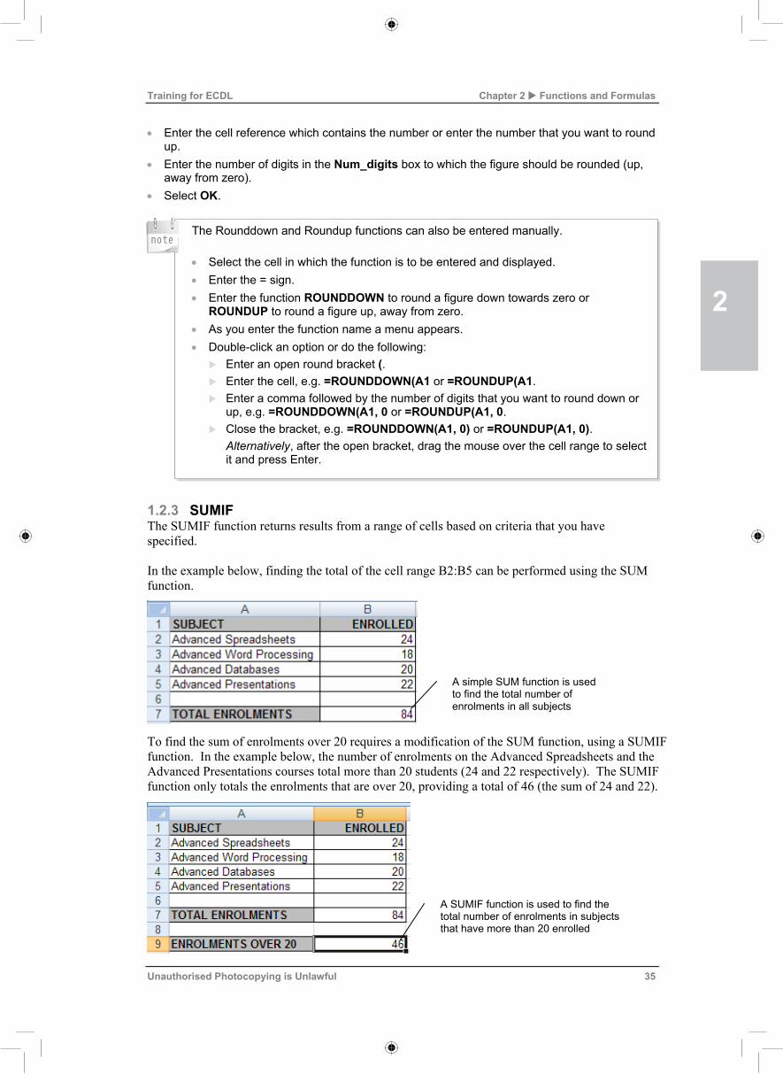
1.2.3 SUMIF The SUMIF function returns results from a range of cells based on criteria that you have specified. In the example below, finding the total of the cell range B2:B5 can be performed using the SUM function.
To find the sum of enrolments over 20 requires a modification of the SUM function, using a SUMIF function. In the example below, the number of enrolments on the Advanced Spreadsheets and the Advanced Presentations courses total more than 20 students (24 and 22 respectively). The SUMIF function only totals the enrolments that are over 20, providing a total of 46 (the sum of 24 and 22).
A simple SUM function is used to find the total number of enrolments in all subjects
A SUMIF function is used to find the total number of enrolments in subjects that have more than 20 enrolled
note

2
Functions and Formulas Chapter 2 Training for ECDL
36 Unauthorised Photocopying is Unlawful
Text or criteria containing mathematical or logical symbols must be enclosed in double “quotation marks”.
The syntax for the SUMIF function above is as follows: =SUMIF(B2:B5, ">20"). All functions must start with the = sign. This is followed by the function name (SUMIF). The function name is followed by an open bracket (. The open bracket is followed by the range, in the example above this is B2:B5. This is followed by the criteria, in the example above this is ">20". The final element is a close bracket ). The Sum_Range are the range of numbers to be totalled. A Sum_Range should only be entered if it differs from the range. If the Sum_Range is omitted from the formula, the cells from the range are used. An example of a SUMIF function using the Sum_Range is shown on the right. In the above example, the syntax for the SUMIF function to find the total of all subjects that contain the word "Advanced" is: =SUMIF(A2:A6, "Advanced*", B2:B6). The range in which the criteria can be found is A2:A6. The criteria (using a wildcard) is Advanced*. The range to sum (for cells corresponding to the criteria) is B2:B6. The enrolment for Improving Productivity is omitted from the result as it does not contain the word ‘Advanced’. To use the SUMIF function, do the following: Click into the cell that is to display the results of the formula. Select the Formulas tab. From the Function Library group, select the Math & Trig arrow. Scroll down the list and select SUMIF.
The Function Arguments window opens. Enter the range to be evaluated.
note
Training for ECDL Chapter 2 Functions and Formulas
Unauthorised Photocopying is Unlawful 37
The SUMIF function can also be entered manually. Select the cell in which the function is to be entered and displayed. Enter the = sign. After the = sign, enter the function SUMIF. As you enter the function name a menu appears. Double-click an option or begin entering the formula.
Examples are shown below: =SUMIF(B3:B6, ">20"). =SUMIF(A3:A6, "Advanced Word Processing", B3:B6). Remember, text or criteria containing mathematical or logical symbols must be enclosed in double “quotation marks”.
Alternatively, click the Collapse Dialog button at the end of the Range box to return to the spreadsheet in order to highlight the range (then click the Restore Dialog button to return to the Function Arguments window).
Enter the criteria. Alternatively, click the Collapse Dialog button at the end of the Criteria box to return to the spreadsheet in order to highlight the criteria if it exists on the worksheet (then click the Restore Dialog button to return to the Function Arguments window).
Enter the sum_range. Alternatively, click the Collapse Dialog button at the end of the Sum_range box to return to the spreadsheet in order to highlight the range on the worksheet (then click the Restore Dialog button to return to the Function Arguments window).
Click OK.
1.3 Statistical Functions (4.2.1.3) Statistical functions include COUNTIF, COUNTBLANK and RANK. 1.3.1 COUNTIF The COUNTIF function returns results from a range of non-blank cells based on a single criterion that you have specified, e.g. count the number of enrolments over 20. For example, a spreadsheet may contain a list of courses which includes the amount of students enrolled on each course. Counting the amount of enrolments on each course can be performed using a straightforward COUNT function, but to count only enrolments that are over 20, a COUNTIF function is required. See the example below:
Collapse Dialog button
The Restore Dialog button appears when the Function Arguments window is collapsed
note

3
Charts Chapter 3 Training for ECDL
86 Unauthorised Photocopying is Unlawful
2.3 Changing Display Units (4.3.2.3) The values on a primary or secondary value axis can be displayed in units of hundreds, thousands or millions without changing the data source. To change display units, do the following: Select the chart. From the Chart Tools/Layout tab and the Axes group, select the Axes command. Select Primary Vertical Axis or Secondary Vertical Axis. Select More Primary Vertical Axis Options (or More Secondary Vertical Axis Options if
applicable). The Format Axis window opens.
Ensure that the Axis Options tab is selected.
Select the Display Units list box arrow. Choose a display unit, e.g. Hundreds,
Thousands, Millions. Click Close.
2.4 Formatting Chart Elements to Display Images (4.3.2.4) To format columns, bars, plot area and chart area to display an image, do the following. Select the chart element to be formatted. (To do this, click the chart
element or select the chart and then select Chart Tools/Format tab and the Current Selection group, select the Chart Elements arrow and then select a chart element from the menu (e.g. data series for a column/bar or plot/chart area).
From the the Chart Tools/Format tab and Current Selection group,
select the Format Selection command. The Format Data Series window opens.
Select the Fill tab. Select the Picture or texture fill option button.
Inserting Pictures from File Under Insert from… select the File…button
The Insert Picture window opens. Select the file location from the Look in: drop-down menu. Select the image file. Click Insert.
Training for ECDL Chapter 3 Charts
Unauthorised Photocopying is Unlawful 87
Select a display option from the following:
Stretch. Stack. Stack and scale with: (and choose the
number of units/pictures to be stacked) Click Close.
The selected data series will display an image with the chosen format. For example:
The Selected data series (Vegetarian Cookery) displays fruit image with Stack format

3
Charts Chapter 3 Training for ECDL
88 Unauthorised Photocopying is Unlawful
When the plot area or chart area is selected, the option to Tile picture as texture becomes available. Select or deselect this box as applicable. Tiling options also become available.
Inserting Pictures from Clipart Under Insert from… select the Clipart button.
The Select Picture window opens. Enter the search word into the Search text box. Click Go (select or deselect the Include content
from Office Online if you want to include/exclude images from Internet sources).
Select an image. Click OK. Select a display option from the following:
Stretch. Stack. Stack and scale with: (and choose the
number of units/pictures to be stacked). Click Close.
note
Select or deselect the tick box as required
Choose a tiling option
Choose an alignment
Choose transparency
Training for ECDL Chapter 3 Charts
Unauthorised Photocopying is Unlawful 89
Practice Sequence
This practice sequence will test you on what you have learned in the previous chapter. In this exercise you will practise re-positioning chart elements, change the scale and major intervals of a value axis, change display units on the value axis and format columns to display an image.
1 Open the Combined Chart spreadsheet that you saved in the last practice sequence. Insert the following chart title Dublin Cookery Class Enrolments so that it displays with Centred Overlay position. If you need help:
Select the chart. From the Chart Tools/Layout tab and the Labels group, select the Chart Title command. From the Chart Title list, select the Centred Overlay position. A Chart Title box appears on the chart in the selected position. Position the cursor within this box and delete the existing text. Enter the chart title.
2 Reposition the chart title so that it displays Above Chart. If you need help:
Select the chart title. From the Chart Tools/Layout tab and the Labels group, select the Chart Title command. From the Chart Title list, select the Above Chart position.
3 Reposition the legend so that it displays at the bottom of the chart. If you need help:
Select the chart. From the Chart Tools/Layout tab and the Labels group, select the Legend command. From the Legend list, select Show Legend at Bottom.
4 Change the minimum scale of the Primary Vertical Axis to 5. If you need help:
Select the chart. From the Chart Tools/Layout tab and the Axes group, select the Axes command. Select Primary Vertical Axis. Select More Primary Vertical Axis Options. The Format Axis box opens. Ensure that the Axis Options tab is selected. Select the Fixed option button for the Minimum scale. Enter 5 for the minimum scale. Click Close.
5 Change the maximum scale of the Primary Vertical Axis to 35. If you need help:
Select the chart. From the Chart Tools/Layout tab and the Axes group, select the Axes command. Select Primary Vertical Axis. Select More Primary Vertical Axis Options. The Format Axis box opens. Ensure that the Axis Options tab is selected. Select the Fixed option button for the Maximum scale. Enter 35 for the maximum scale. Click Close.
6 Change the Major Interval units on the Primary Vertical Axis to 10. If you need help:
Select the chart. From the Chart Tools/Layout tab and the Axes group, select the Axes command. Select Primary Vertical Axis. Select More Primary Vertical Axis Options. The Format Axis box opens. Ensure that the Axis Options tab is selected. Select the Fixed option button for the Major Unit scale. Enter 10 for the major unit. Click Close.
7 Change the display units on the Primary Vertical Axis to Hundreds. If you need help:
Select the chart. From the Chart Tools/Layout tab and the Axes group, select the Axes command. Select Primary Vertical Axis. Select More Primary Vertical Axis Options. The Format Axis box opens. Ensure that the Axis Options tab is selected. Select the Display Units arrow and select Hundreds. Click Close.
8 Change the Vegetarian Cookery data series to a column chart type. See previous practice sequence for instructions. Format the Vegetarian Cookery data series to display the image Fruit.gif and display with a Stack format. If you need help:
Select the Vegetarian Cookery data series. From the the Chart Tools/Format tab and Current Selection group, select the Format Selection command. The Format Data Series window opens. Select the Fill tab. Select the Picture or texture fill option button. Under Insert from… select the File… button. The Insert Picture window opens. Select the file location from the Look in: drop-down menu. Select the image file Fruit.gif and click Insert. Select the Stack display option. Click Close.
9 Save the spreadsheet and close.

3
Charts Chapter 3 Training for ECDL
90 Unauthorised Photocopying is Unlawful
1 A combined chart can include which of the following?
6 What is the default position of a chart legend?
2-D column and line.
3-D column and line.
Right.
Left.
Top.
Bottom.
2 A secondary axis is useful for which of the following reasons?
7 Which of the following statements best describes a legend?
To distinguish data from different data series in a combined column/line chart.
To view data in a column chart based on a single data series.
It is the key which identifies data series within a chart.
It displays units of hundreds, thousands or millions.
3 The chart type of a defined data series in a 2-D column chart can be changed by doing which of the following?
8 What is a major unit?
Selecting the chart area and then selecting Change Chart Type.
Selecting the plot area and then selecting Change Chart Type.
Selecting the vertical value axis and then selecting Change Chart Type.
Selecting the data series and then selecting Change Chart Type.
The difference between the minimum and maximum numbers.
The interval between each number on a value scale.
The maximum number on a value scale.
4 A data series can be deleted from a chart without deleting the associated spreadsheet data. True or false?
9 To format a column/bar or plot area or chart area to display an image, which of the following actions would you perform?
True.
False.
Select the chart element and then select the Picture command from the Insert tab.
Select the chart element and then select the Format Selection command from the Chart Tools/Format tab.
5 To add a data series to a chart, the data must already exist in the data source. True or false?
10 To change the display units on a value axis to hundreds, thousands or millions you must change the data source. True or false?
True.
False.
True.
False.
Self-Check Exercises
Training for ECDL Chapter 3 Charts
Unauthorised Photocopying is Unlawful 91
Practice Sequence Complete the following exercises as a review of the topics covered in this chapter. Should you require assistance with any of the steps within these exercises, refer back to the corresponding sections within this chapter.
Exercise 1
1 Create a new spreadsheet. Create a combined column/ line chart (with a 2-D column chart type and a line with markers chart type) from the following data.
2 Add a Year 3 data series to the chart from the data below.
Year 3 25000 36000 30000
3 Remove the Year 1 data series from the chart.
4 Change the Year 2 data series to a 2-D column chart type.
5 To make it easier to distinguish between values in the two data series, add a secondary axis to the combined chart.
6 Change the scale of the Primary Vertical Axis to the following: Minimum 0 and the Maximum 50000.
7 Change the major unit for the Secondary Vertical Axis so that the interval between each value is 10000.
8 Display Thousand units on the Secondary Vertical Axis.
9 Reposition the legend to appear on the left-hand side of the chart.
10 Format the chart area to display the image Background.png
11 Save the spreadsheet file as Food_book_sales.xlsx and close.

4
Analysis Chapter 4 Training for ECDL
132 Unauthorised Photocopying is Unlawful
Method 2 Enter values on the spreadsheet in the order that you want the data sorted (the values can be
deleted once the custom list is created). For example:
Highlight the sort values. Select the Office Button and then select Excel Options.
The Excel Options window opens. In the Popular tab, in the Top Options for working with Microsoft Excel section, click the
Edit Custom Lists button. The Custom Lists window opens.
Select the Import button. The new list entries will be displayed in the Custom Lists section.
Click OK to close the Custom Lists window. Click OK again to return to the spreadsheet. Select the data range to be sorted.
2.2.3 Applying a Custom List To apply a custom list to selected data, do the following: From the Data tab and the Sort & Filter group, select the Sort command.
The Sort window opens. Select the field to sort by from the Column drop-down list. Select Values from the Sort On drop-down list. Select Custom List from the Order drop-down list.
The Custom Lists window opens. Select the new custom sort order from the Custom Lists. Click OK to close the Custom Lists window. Click OK again to return to the spreadsheet.
2.2.4 Deleting a Custom List To delete a custom list, do the following: Select the Office Button and then select Excel Options.
The Excel Options window opens. In the Popular window, in the Top Options for working with Microsoft Excel section, click
the Edit Custom Lists button. The Custom Lists window opens.
Select the custom list to be deleted from the Custom Lists section of the window. Click Delete. Click OK to confirm deletion of the custom list. Click OK to close the window. Click OK again to return to the spreadsheet.
2.3 Filtering a List in Place (4.4.2.3) Data can be filtered in its current position on the spreadsheet to display a subset of data. This is referred to as an AutoFilter. For example, a list of leisure courses can be filtered to display only Swimming courses.
High Medium Low
Low Medium High
Training for ECDL Chapter 4 Analysis
Unauthorised Photocopying is Unlawful 133
2.3.1 Text Filters To create a text filter, do the following: Select the data to be filtered or click anywhere within the data range. From the Data tab and the Sort & Filter group, select the Filter command. Filter arrows are displayed for each of the column headings within the selected data.
The data in the example below is unfiltered.
Select a filter arrow and, from the Filter pane, deselect (clear) or select
data item tick boxes (e.g. select only Swimming tick box to filter the data and display only Swimming courses). The filter arrow changes to indicate that the column is filtered.
Alternatively, select Text Filters and then select a comparison operator from the sub-menu:

4
Analysis Chapter 4 Training for ECDL
134 Unauthorised Photocopying is Unlawful
Below is an explanation of comparison operators.
Comparison Operator Action Comparison
Operator Action
Equals Will find data that matches the criteria. For example, Equals Swimming will extract only Swimming courses.
Does Not Equal
Will find data not matching the criteria. For example, Does Not Equal Swimming will find all courses except the Swimming courses.
Begins With
Will find data that begins with a specified character. For example, Begins With C will extract courses beginning with C (Circuit Training, etc.).
Ends With
Will find data that ends with a specified character. For example, Ends With G will extract courses ending in this character (swimming, Circuit Training, etc.).
Contains Will find data based on specified characters that are specified. For example, Contains W will find courses that contain this character (e.g. Swimming, Water Aerobics).
Does Not Contain Will filter all data except for all courses containing the specified character (e.g. If W is specified as the criteria, the filtered data would not include (swimming, or Water Aerobics, etc.).
The Custom AutoFilter window opens. The first drop-down list in the window will display the chosen comparison operator. To change the comparison operator, select the list arrow and choose an option from the menu.
Choose the required data item from the parallel drop-down list (a data item is each piece of data within a field). For example, a leisure courses table may include a COURSE field which in turn may contain data items such as Swimming, Circuit Training, etc. Alternatively, enter criteria into the box (e.g. type swimming).
Choose the And/Or option button to add further criteria to the filter. Select a further comparison operator and enter or select criteria as required. Click OK.
In the example on the next page, courses containing the character c and not containing the character g should be filtered and displayed. Because AND is used, it restricts the filter to finding only Ice Hockey courses because Circuit Training contains the character g.
Training for ECDL Chapter 4 Analysis
Unauthorised Photocopying is Unlawful 135
In the following example, courses containing the character c or not containing the character g should be filtered and displayed. Because OR is used, the filter displays both Ice Hockey and Circuit Training courses, but not Swimming.
Unfiltered data source
Comparison operator Contains is selected in order to find courses containing the character C
Comparison operator Does not contain is selected in order to find courses not containing the character G
The AND operator is
selected
Both courses contain the character c. Circuit
Training also contains the character g, but
because the OR operator is selected, both courses
are displayed
The OR operator is
selected
Comparison operator Does not contain is selected in order to find courses not containing the character G
Comparison operator Contains is selected in order to find courses containing the character C

4
Analysis Chapter 4 Training for ECDL
136 Unauthorised Photocopying is Unlawful
Wildcards Wildcards are characters such as ? and * that are used to represent a single character (?) within a field or any series of characters within a field (*). For example: Contains *I* will filter and extract data that matches fields containing the character I. Entering S?i??ing will filter and extract data that matches fields containing the specified
characters – e.g. swimming. The ? wildcard character represents the missing characters. For example: A spreadsheet contains data relating to leisure courses: Swimming, Circuit Training and Ice Hockey. A custom autofilter is applied to filter courses that contain the character i AND do not contain the character k. A wildcard (*) is used to represent the missing characters. The following courses are filtered and extracted: Swimming and Circuit Training (they both contain the character i as specified). Ice Hockey is not displayed as, although it matches the contains criteria (i), it also contains the does not contain criteria k. However, if the OR operator is selected, all of the courses would be displayed (swimming, circuit training and ice hockey all match the first set of criteria). 2.3.2 Number Filters To create a number filter, do the following: Select the data to be filtered. From the Data tab and the Sort & Filter group, select the Filter command. Filter arrows are displayed for each of the column headings within the selected data.
Select a filter arrow. From the Filter pane, deselect (clear) or select data
item tick boxes. The filter arrow changes to indicate that the column is filtered.
Will find any course containing the character i …
… AND will find any course not containing the character k
Training for ECDL Chapter 4 Analysis
Unauthorised Photocopying is Unlawful 137
Alternatively, select Number Filters and then select a comparison operator from the sub-menu.
See explanation of comparison operators below. Comparison Operator Action Comparison
Operator Action
Greater Than
Will find data that is greater than the specified value. For example, Greater Than 3 will extract courses with more than 3 sessions.
Greater Than Or Equal To
Will find data that is greater than or equal to the specified value. For example, Greater Than Or Equal To 3 will extract courses with 3 or more sessions.
Less Than
Will find data that is less than the specified value. For example, Less Than 3 will extract courses with less than 3 sessions.
Less Than Or Equal To
Will find data that is less than or equal to the specified value. For example, Less Than Or Equal To 3 will extract courses with 3 or less sessions.
Between
Will find data that is between 2 specified values. For example, Between 2 And 4 will extract courses with sessions between these two figures (will find 2, 3 and 4) and Between 01/01/2010 And 31/12/2010 will find dates between the specified start/end date.
Top 10 Will find the specified amount of top or bottom items, percents or sums specified by you.
Above Average
Will find and filter data that is above average.
Below Average Will find and filter data that is below average.
Using Comparison Operators To use the Greater Than, Greater Than Or Equal To, Less Than, Less Than Or Equal To and Between comparison operators in a filter, do the following: Select a comparison operator from the Number Filter sub-menu.
The Custom AutoFilter window opens.
Select a comparison operator

5
Validating and Auditing Chapter 5 Training for ECDL
166 Unauthorised Photocopying is Unlawful
1.1.1. Setting and Editing Validation Criteria To set and/or edit validation criteria, do the following: Select the cell or cell range to which the validation criteria is to be applied. From the Data tab and the Data Tools group, select the Data Validation
command. Do not click the list arrow unless you want to select an option from the drop-down menu. The Data Validation window opens.
Ensure that the Settings tab is selected. Select the Allow: list arrow under Validation Criteria and choose an option from the drop-
down menu.
Click OK. 1.1.2 Setting Validation Criteria for Whole or Decimal Numbers To set validation criteria for data entry in a cell range to restrict entry of whole or decimal numbers, do the following: Select the cell or cell range to which the validation criteria is to be applied. From the Data tab and the Data Tools group, select the Data Validation
command. Do not click the list arrow unless you want to select an option from the drop-down menu. The Data Validation window opens.
Ensure that the Settings tab is selected. Select Whole number or Decimal from the Allow: list arrow under Validation Criteria. Select the Data list arrow and choose a comparison operator from the following:
Between – will find numbers between a specified minimum and maximum number (e.g. between minimum 10 and maximum 20 will only allow data between these two numbers to be entered (inclusive).
Not between – will find numbers either side of the specified minimum and maximum number ((e.g. not between minimum 10 and maximum 20 will not allow data between these two numbers to be entered (inclusive).
Choose an option from the drop-down list
Training for ECDL Chapter 5 Validating and Auditing
Unauthorised Photocopying is Unlawful 167
Equal to – will only allow a specified number to be entered (e.g. Equal to 10 will only allow entry of number equal to 10).
Not equal to - will not allow a specified number to be entered (e.g. Not equal to 10 will allow entry of any number other than 10).
Greater than – will allow entry data greater than a specified number (e.g. greater than 10 will restrict users to enter numbers greater than 10)
Less than - will allow entry of data less than a specified number (e.g. less than 10 will restrict users to enter numbers that are below 10)
Greater than or equal to - will allow entry of data greater than or equal to a specified number (e.g. greater than or equal to 10 will restrict users to enter numbers that equal 10 or over. Will allow 10, 21, 32, 43 etc, but not 9)
Less than or equal to - will allow entry of data less than or equal to a specified number (e.g. less than or equal to 10 will restrict users to enter numbers that are 10 or below)
Enter a minimum number in the Minimum box or select the Collapse Dialog button and select the data in the spreadsheet. Select the Expand Dialog button to return to the window.
Enter a maximum, number in the Maximum box or select the Collapse Dialog button and select the data in the spreadsheet. Select the Expand Dialog button to return to the window.
Select or deselect the Ignore blank tick box to ignore or include blank cells in the validation. When the Ignore blank check box is selected it allows any value to be entered into a blank cell, unrestricted by data validation. If you want to apply the validation criteria to all other cells in the spreadsheet that share the same settings, select the tick box.
Click OK. When invalid data, not matching the
validation criteria, is entered in a cell, the following default error message appears.
Click Cancel to re-enter data that match the validation criteria.
1.1.3 Setting Validation Criteria for Lists Data within a drop-down menu can be taken from other cells within the worksheet or from cells within a different worksheet or entered directly into the Source box in the Data Validation window. Data entered into the Source box must be separated by a comma. For example, a drop-down list that asks a specific question may include the following data items: Yes, No.
Select this to ignore blank cells or deselect to include blank cells

5
Validating and Auditing Chapter 5 Training for ECDL
168 Unauthorised Photocopying is Unlawful
To set validation criteria so that users are restricted to choosing data from a drop-down list, do the following: Entering List Items Manually Select the cell where the drop down list is to be located on the spreadsheet. Open the Data Validation window and the Settings tab. Select List from the Allow: list arrow under Validation Criteria. Click into the Source box and enter the items that should be included in the drop-down list.
Ensure that the data items are separated by a comma, e.g. Yes, No:
Select or deselect the Ignore blank tick box to ignore or include blank cells in the validation. In order to see the drop-down list arrow, ensure that the In-cell dropdown tick box is selected.
If you want to apply the validation criteria to all other cells in the spreadsheet that share the same settings, select the tick box.
Click OK. A list arrow is displayed in the selected cell. When the arrow is clicked a drop-down list appears, displaying the specified data.
Click a list item to enter it into the cell. When invalid data, not matching an
item within the drop-down list, is entered in a cell, an error message opens.
Click Cancel to re-enter or select data that matches the validation criteria.
Separate list items with a comma
Training for ECDL Chapter 5 Validating and Auditing
Unauthorised Photocopying is Unlawful 169
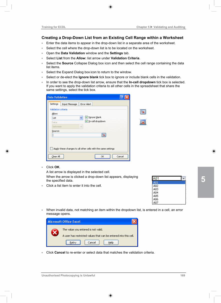
Creating a Drop-Down List from an Existing Cell Range within a Worksheet Enter the data items to appear in the drop-down list in a separate area of the worksheet. Select the cell where the drop-down list is to be located on the worksheet. Open the Data Validation window and the Settings tab. Select List from the Allow: list arrow under Validation Criteria. Select the Source Collapse Dialog box icon and then select the cell range containing the data
list items. Select the Expand Dialog box icon to return to the window. Select or de-elect the Ignore blank tick box to ignore or include blank cells in the validation. In order to see the drop-down list arrow, ensure that the In-cell dropdown tick box is selected.
If you want to apply the validation criteria to all other cells in the spreadsheet that share the same settings, select the tick box.
Click OK. A list arrow is displayed in the selected cell. When the arrow is clicked a drop-down list appears, displaying the specified data.
Click a list item to enter it into the cell. When invalid data, not matching an item within the dropdown list, is entered in a cell, an error
message opens.
Click Cancel to re-enter or select data that matches the validation criteria.
5
Validating and Auditing Chapter 5 Training for ECDL
168 Unauthorised Photocopying is Unlawful
To set validation criteria so that users are restricted to choosing data from a drop-down list, do the following: Entering List Items Manually Select the cell where the drop down list is to be located on the spreadsheet. Open the Data Validation window and the Settings tab. Select List from the Allow: list arrow under Validation Criteria. Click into the Source box and enter the items that should be included in the drop-down list.
Ensure that the data items are separated by a comma, e.g. Yes, No:
Select or deselect the Ignore blank tick box to ignore or include blank cells in the validation. In order to see the drop-down list arrow, ensure that the In-cell dropdown tick box is selected.
If you want to apply the validation criteria to all other cells in the spreadsheet that share the same settings, select the tick box.
Click OK. A list arrow is displayed in the selected cell. When the arrow is clicked a drop-down list appears, displaying the specified data.
Click a list item to enter it into the cell. When invalid data, not matching an
item within the drop-down list, is entered in a cell, an error message opens.
Click Cancel to re-enter or select data that matches the validation criteria.
Separate list items with a comma
Training for ECDL Chapter 5 Validating and Auditing
Unauthorised Photocopying is Unlawful 169
Creating a Drop-Down List from an Existing Cell Range within a Worksheet Enter the data items to appear in the drop-down list in a separate area of the worksheet. Select the cell where the drop-down list is to be located on the worksheet. Open the Data Validation window and the Settings tab. Select List from the Allow: list arrow under Validation Criteria. Select the Source Collapse Dialog box icon and then select the cell range containing the data
list items. Select the Expand Dialog box icon to return to the window. Select or de-elect the Ignore blank tick box to ignore or include blank cells in the validation. In order to see the drop-down list arrow, ensure that the In-cell dropdown tick box is selected.
If you want to apply the validation criteria to all other cells in the spreadsheet that share the same settings, select the tick box.
Click OK. A list arrow is displayed in the selected cell. When the arrow is clicked a drop-down list appears, displaying the specified data.
Click a list item to enter it into the cell. When invalid data, not matching an item within the dropdown list, is entered in a cell, an error
message opens.
Click Cancel to re-enter or select data that matches the validation criteria.

5
Validating and Auditing Chapter 5 Training for ECDL
170 Unauthorised Photocopying is Unlawful
Creating a Drop-Down List from a Defined Name Cell Range from a Different Worksheet Open a separate worksheet. Enter the data items to appear in the drop-down list within the worksheet. Select the data items. Select the Formulas tab. Select the Define Names command from the Defined Names group.
The New Name window opens. Enter a name for the selected cell range. Click OK to close the New Name window. Return to the worksheet to contain the drop-down list. Select the cell where the drop-down list is to be located.
Open the Data Validation window and the Settings tab. Select List from the Allow: list arrow under Validation Criteria. Click into the Source box and enter the
defined name (enter the equals sign = before the defined name, e.g. =Sales_ID).
Select or deselect the Ignore blank tick box to ignore or include blank cells in the validation. In order to see the drop-down list arrow, ensure that the In-cell dropdown tick box is selected.
If you want to apply the validation criteria to all other cells in the spreadsheet that share the same settings, select the tick box.
Click OK. A list arrow is displayed in the selected cell. When the arrow is clicked a drop down list appears, displaying the specified data.
Click a list item to enter it into the cell. When invalid data, not matching an item within the drop-down list, is entered in a cell, an error message opens.
Click Cancel to re-enter or select data that matches the validation criteria.
Training for ECDL Chapter 5 Validating and Auditing
Unauthorised Photocopying is Unlawful 171
1.1.4 Setting Validation Criteria for Dates/Times To set validation criteria, so that users are restricted to entering dates or times that match the criteria, do the following: Select the cell or cell range to which the validation criteria is to be applied. Open the Data Validation window and the Settings tab. Select Date or Time from the Allow: list arrow under Validation Criteria. Select a comparison operator from the Data list. For example, Between specified start and
specified end date/time (see Section 1.1.2 for examples of comparison operators). Enter a start date or a start time in the Start date or Start time box.
Alternatively, click the Collapse Dialog button to return to the spreadsheet and highlight the date/time. Click the Expand Dialog button to return to the window.
Enter an end date or an end time in the End Date or the End time box. Alternatively, click the Collapse Dialog button to return to the spreadsheet and highlight the date/time. Click the Expand Dialog button to return to the window.
Select or deselect the Ignore blank tick box to ignore or include blank cells in the validation.
Click OK. When an invalid date or time, not matching the validation criteria, is entered in a cell, an error
message opens.
Click Cancel to re-enter a date or time that matches the validation criteria.
1.1.5 Setting Validation Criteria for Text Length To set validation criteria, so that users are restricted to entering text that matches the length specified in the validation criteria, do the following: Select the cell or cell range to which the validation criteria is to be applied. Open the Data Validation window and the Settings tab. Select Text Length from the Allow: list arrow under Validation Criteria. Select a comparison operator from the Data list. For example, Between specified text lengths
(see Section 1.1.2 for examples of comparison operators).

6
Enhancing Productivity Chapter 6 Training for ECDL
210 Unauthorised Photocopying is Unlawful
4.1.1 Inserting a Hyperlink To insert a hyperlink, do the following: Within a Spreadsheet Select the cell which is to contain the hyperlink. From the Insert tab and the Links group, select the Hyperlink command.
The Insert Hyperlink window opens. Ensure that Place in This Document is selected in the Link to: list. Click into the Text to display: box and enter the text that is to be displayed as the hyperlink
text. Select the ScreenTip… button to add or change the text that will be displayed when the cursor
is hovered over the hyperlink. Type in the cell reference or select a place in a specific worksheet (hyperlinks can also be
applied to defined named cell ranges within the spreadsheet).
Click OK to return to the spreadsheet.
The hyperlink text will be displayed with a blue underline. When the cursor is hovered over the hyperlink, it turns into a white hand icon and the ScreenTip appears detailing the location of the hyperlink.
Click the mouse to follow the link. To a Different Spreadsheet or File Select the cell that is to contain the hyperlink. From the Insert tab and the Links group, select the Hyperlink command. Ensure that Existing File or Web Page is selected in the Link to: list. Click into the Text to display: box and enter the text that is to be displayed as
the hyperlink text. Select the ScreenTip… button to add or change the text that will be displayed
when the cursor is hovered over the hyperlink.
Training for ECDL Chapter 6 Enhancing Productivity
Unauthorised Photocopying is Unlawful 211
Choose the correct drive/folder from the Look in: drop-down menu. Select a spreadsheet file from the list.
To create a hyperlink to a specific location within the selected spreadsheet,
select the Bookmark button. The Select Place in Document window opens.
Type in the cell reference or select a place in a specific worksheet (hyperlinks can also be applied to defined named cell ranges within the spreadsheet).
Click OK to return to the Insert Hyperlink window. The hyperlink location will be displayed in the Address box.
Click OK. The hyperlink text will be displayed with a blue underline. When the cursor is hovered over the hyperlink, it turns into a white hand icon and the ScreenTip appears detailing the location of the hyperlink.
Click the mouse to follow the link.
6
Enhancing Productivity Chapter 6 Training for ECDL
212 Unauthorised Photocopying is Unlawful
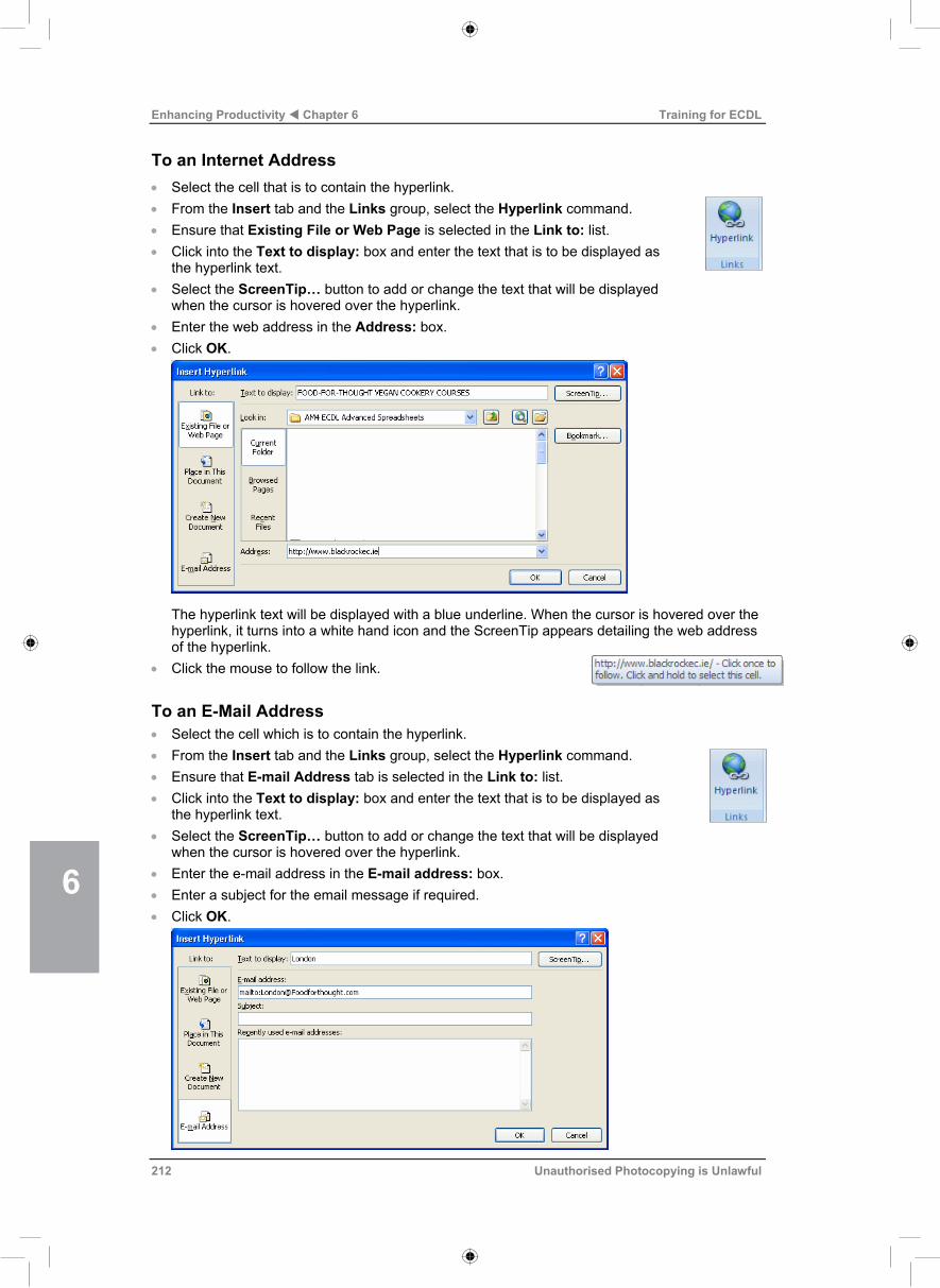
To an Internet Address Select the cell that is to contain the hyperlink. From the Insert tab and the Links group, select the Hyperlink command. Ensure that Existing File or Web Page is selected in the Link to: list. Click into the Text to display: box and enter the text that is to be displayed as
the hyperlink text. Select the ScreenTip… button to add or change the text that will be displayed
when the cursor is hovered over the hyperlink. Enter the web address in the Address: box. Click OK.
The hyperlink text will be displayed with a blue underline. When the cursor is hovered over the hyperlink, it turns into a white hand icon and the ScreenTip appears detailing the web address of the hyperlink.
Click the mouse to follow the link. To an E-Mail Address Select the cell which is to contain the hyperlink. From the Insert tab and the Links group, select the Hyperlink command. Ensure that E-mail Address tab is selected in the Link to: list. Click into the Text to display: box and enter the text that is to be displayed as
the hyperlink text. Select the ScreenTip… button to add or change the text that will be displayed
when the cursor is hovered over the hyperlink. Enter the e-mail address in the E-mail address: box. Enter a subject for the email message if required. Click OK.
Training for ECDL Chapter 6 Enhancing Productivity
Unauthorised Photocopying is Unlawful 213
The hyperlink text will be displayed with a blue underline. When the cursor is hovered over the hyperlink, it turns into a white hand icon and the ScreenTip appears detailing the e-mail address of the hyperlink.
Click the mouse to follow the link. To a New Document Select the cell which is to contain the hyperlink. From the Insert tab and the Links group, select the Hyperlink command. Ensure that Create New Document is selected in the Link to: list. Click into the Text to display: box and enter the text that is to be displayed as
the hyperlink text. Select the ScreenTip… button to add or change the text that will be displayed
when the cursor is hovered over the hyperlink. Change the drive/folder location if required by selecting the Change button and then selecting
a new location. Enter a name for the new file. Choose an option button for one of the following:
Edit the new document later. Edit the new document now.
Click OK. The hyperlink text will be displayed with a blue underline. When the mouse is hovered over the hyperlink, the mouse pointer turns into a white hand icon and the ScreenTip appears detailing the location of the hyperlink.
Click the mouse to follow the link. 4.1.2 Editing a Hyperlink To edit a hyperlink, do the following: Select the cell containing the hyperlink (ensure that you don't click directly on the hyperlink text
or you will open the hyperlink). From the Insert tab and the Links group, select the Hyperlink command.
The Edit Hyperlink window opens. Edit the existing hyperlink by changing the spreadsheet file and/or location within the
spreadsheet or by changing the email address or web address. Click OK.

6
Enhancing Productivity Chapter 6 Training for ECDL
212 Unauthorised Photocopying is Unlawful
To an Internet Address Select the cell that is to contain the hyperlink. From the Insert tab and the Links group, select the Hyperlink command. Ensure that Existing File or Web Page is selected in the Link to: list. Click into the Text to display: box and enter the text that is to be displayed as
the hyperlink text. Select the ScreenTip… button to add or change the text that will be displayed
when the cursor is hovered over the hyperlink. Enter the web address in the Address: box. Click OK.
The hyperlink text will be displayed with a blue underline. When the cursor is hovered over the hyperlink, it turns into a white hand icon and the ScreenTip appears detailing the web address of the hyperlink.
Click the mouse to follow the link. To an E-Mail Address Select the cell which is to contain the hyperlink. From the Insert tab and the Links group, select the Hyperlink command. Ensure that E-mail Address tab is selected in the Link to: list. Click into the Text to display: box and enter the text that is to be displayed as
the hyperlink text. Select the ScreenTip… button to add or change the text that will be displayed
when the cursor is hovered over the hyperlink. Enter the e-mail address in the E-mail address: box. Enter a subject for the email message if required. Click OK.
Training for ECDL Chapter 6 Enhancing Productivity
Unauthorised Photocopying is Unlawful 213
The hyperlink text will be displayed with a blue underline. When the cursor is hovered over the hyperlink, it turns into a white hand icon and the ScreenTip appears detailing the e-mail address of the hyperlink.
Click the mouse to follow the link. To a New Document Select the cell which is to contain the hyperlink. From the Insert tab and the Links group, select the Hyperlink command. Ensure that Create New Document is selected in the Link to: list. Click into the Text to display: box and enter the text that is to be displayed as
the hyperlink text. Select the ScreenTip… button to add or change the text that will be displayed
when the cursor is hovered over the hyperlink. Change the drive/folder location if required by selecting the Change button and then selecting
a new location. Enter a name for the new file. Choose an option button for one of the following:
Edit the new document later. Edit the new document now.
Click OK. The hyperlink text will be displayed with a blue underline. When the mouse is hovered over the hyperlink, the mouse pointer turns into a white hand icon and the ScreenTip appears detailing the location of the hyperlink.
Click the mouse to follow the link. 4.1.2 Editing a Hyperlink To edit a hyperlink, do the following: Select the cell containing the hyperlink (ensure that you don't click directly on the hyperlink text
or you will open the hyperlink). From the Insert tab and the Links group, select the Hyperlink command.
The Edit Hyperlink window opens. Edit the existing hyperlink by changing the spreadsheet file and/or location within the
spreadsheet or by changing the email address or web address. Click OK.
7
Collaborative Editing Chapter 7 Training for ECDL
236 Unauthorised Photocopying is Unlawful
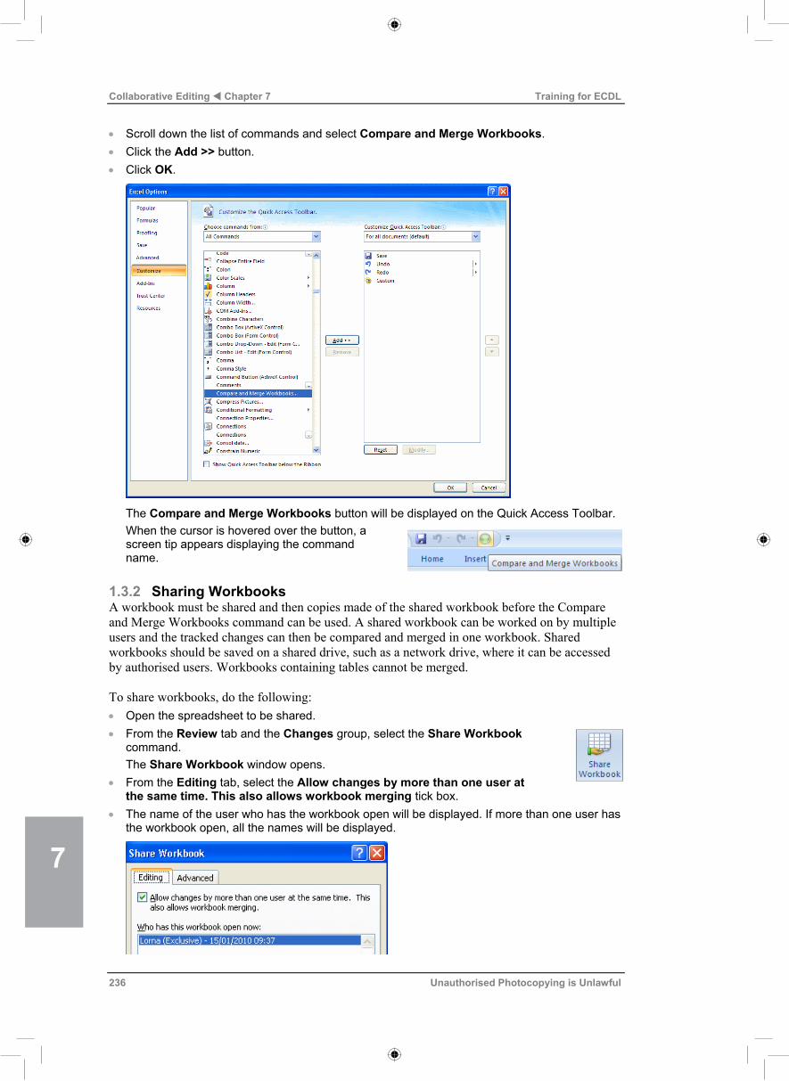
Scroll down the list of commands and select Compare and Merge Workbooks. Click the Add >> button. Click OK.
The Compare and Merge Workbooks button will be displayed on the Quick Access Toolbar. When the cursor is hovered over the button, a screen tip appears displaying the command name.
1.3.2 Sharing Workbooks A workbook must be shared and then copies made of the shared workbook before the Compare and Merge Workbooks command can be used. A shared workbook can be worked on by multiple users and the tracked changes can then be compared and merged in one workbook. Shared workbooks should be saved on a shared drive, such as a network drive, where it can be accessed by authorised users. Workbooks containing tables cannot be merged. To share workbooks, do the following: Open the spreadsheet to be shared. From the Review tab and the Changes group, select the Share Workbook
command. The Share Workbook window opens.
From the Editing tab, select the Allow changes by more than one user at the same time. This also allows workbook merging tick box.
The name of the user who has the workbook open will be displayed. If more than one user has the workbook open, all the names will be displayed.
Training for ECDL Chapter 7 Collaborative Editing
Unauthorised Photocopying is Unlawful 237
Select the Advanced tab. From this window you can choose the following:
The number of days that the tracked changes will be displayed.
How to update changes: when the file is saved or automatically for a specified number of minutes. If using the latter option, also choose whether to save your own changes in addition to seeing other users' changes or opt to see only other users' changes.
How to prioritise conflicting changes between users: ask to be prompted which changes should be prioritised or choose to always prioritise saved changes.
Settings to include in personal view: Print settings and/or filter settings.
Click OK. Copies of the workbook can now be made
by other users, in order to make changes. To make a copy of a shared workbook, do the following: Select Save As from the Office Button.
The Save As window opens. Choose the stored location from the Save in: drop-down menu. Enter a name for the copied workbook (it must differ from the original file name). Click Save.
Protecting and Sharing Workbooks To ensure that tracked changes cannot be turned off by other users of a shared workbook, it can be protected with a password. To share and protect a workbook, do the following: Open the spreadsheet to be shared. From the Review tab and the Changes group,
select the Protect and Share Workbook command. The Protect Shared Workbook window opens.
Select the Sharing with track changes tick box. If required, enter a password into the Password (optional) box. Click OK.
If a password was entered, the Confirm Password window opens.

7
Collaborative Editing Chapter 7 Training for ECDL
236 Unauthorised Photocopying is Unlawful
Scroll down the list of commands and select Compare and Merge Workbooks. Click the Add >> button. Click OK.
The Compare and Merge Workbooks button will be displayed on the Quick Access Toolbar. When the cursor is hovered over the button, a screen tip appears displaying the command name.
1.3.2 Sharing Workbooks A workbook must be shared and then copies made of the shared workbook before the Compare and Merge Workbooks command can be used. A shared workbook can be worked on by multiple users and the tracked changes can then be compared and merged in one workbook. Shared workbooks should be saved on a shared drive, such as a network drive, where it can be accessed by authorised users. Workbooks containing tables cannot be merged. To share workbooks, do the following: Open the spreadsheet to be shared. From the Review tab and the Changes group, select the Share Workbook
command. The Share Workbook window opens.
From the Editing tab, select the Allow changes by more than one user at the same time. This also allows workbook merging tick box.
The name of the user who has the workbook open will be displayed. If more than one user has the workbook open, all the names will be displayed.
Training for ECDL Chapter 7 Collaborative Editing
Unauthorised Photocopying is Unlawful 237
Select the Advanced tab. From this window you can choose the following:
The number of days that the tracked changes will be displayed.
How to update changes: when the file is saved or automatically for a specified number of minutes. If using the latter option, also choose whether to save your own changes in addition to seeing other users' changes or opt to see only other users' changes.
How to prioritise conflicting changes between users: ask to be prompted which changes should be prioritised or choose to always prioritise saved changes.
Settings to include in personal view: Print settings and/or filter settings.
Click OK. Copies of the workbook can now be made
by other users, in order to make changes. To make a copy of a shared workbook, do the following: Select Save As from the Office Button.
The Save As window opens. Choose the stored location from the Save in: drop-down menu. Enter a name for the copied workbook (it must differ from the original file name). Click Save.
Protecting and Sharing Workbooks To ensure that tracked changes cannot be turned off by other users of a shared workbook, it can be protected with a password. To share and protect a workbook, do the following: Open the spreadsheet to be shared. From the Review tab and the Changes group,
select the Protect and Share Workbook command. The Protect Shared Workbook window opens.
Select the Sharing with track changes tick box. If required, enter a password into the Password (optional) box. Click OK.
If a password was entered, the Confirm Password window opens.

7
Collaborative Editing Chapter 7 Training for ECDL
238 Unauthorised Photocopying is Unlawful
Re-enter the password to proceed. Click OK.
A message window opens.
Click OK to continue saving the workbook. 1.3.3 Comparing and Merging Workbooks To compare changes made between multiple shared workbooks, do the following: Open the original shared workbook. Select the Compare and Merge Workbooks button.
The Select Files to Merge into Current Workbook window opens. Select the file location from the Look in: drop-down menu. Select the file to be merged. Click OK.
The changes made in the selected shared workbook will be compared and merged with the current workbook.
Save the merged workbook.
Training for ECDL Chapter 7 Collaborative Editing
Unauthorised Photocopying is Unlawful 239
Practice Sequence
1 Open the spreadsheet entitled Marquee_hire.xlsx. Track the following changes made to the following cell range only B4:D6. Change the Daily Hire for 2009 to 26,000. Change the Weekly Hire for 2009 to 37,500. If you need help: From the Review Tab and the Changes group, select the Track Changes arrow. Select Highlight Changes… from the drop-down menu. The Highlight Changes window opens. Select the Track changes while editing tick box. In the Highlight which changes section, select the When tick box and then select the list arrow. Choose All from the list. Select the Who tick box and then select the list arrow. Choose Everyone from the list. Select the Where tick box and then select the Collapse Dialog button. Choose B4:D6 as the area of the spreadsheet that should be tracked. Select the Highlight changes on screen tick box. Click OK. You will be prompted to resave the workbook; click OK. The workbook is saved as a shared workbook. Any changes made to the spreadsheet data will be tracked and highlighted.
2 Continue working on the Marquee_hire (Shared).xlsx spreadsheet. Reject the following change made to the cell range B4:D6. Change the Daily Hire for 2009 to 26,000. Accept the following change made to the cell range B4:D6. Change the Weekly Hire for 2009 to 37,500. Save and close the workbook. If you need help: From the Review Tab and the Changes group, select the Track Changes arrow. Select Accept/Reject Changes. A message will prompt you to save the workbook. Click OK. The Select Changes to Accept or Reject window opens. Select When, Who and Where options as appropriate and click OK. The Accept or Reject Changes window opens. Select the Reject button to reject the displayed change. Select the Accept button to accept the displayed change. Click Close.
3 Save this workbook (it will be saved as a shared workbook) and make a copy with the name Marquee_hire(2).xlsx. If you need help: Select Save As from the Office Button. Enter the specified file name and click Save.
4 Continue working on the shared copied spreadsheet entitled Marquee_hire(2).xlsx. Track the following changes made to the cell range B10:D14. Change the Equipment costs for 2009 to 25,000. Change the Catering costs for 2009 to 4,000. Save and close the workbook.
5 Open the spreadsheet entitled Marquee_hire.xlsx. Compare and merge the changes made to the copied workbook Marquee_hire(2) with the original workbook Marquee_hire. Save the workbook and close. If you need help: Open the original shared workbook entitled Marquee_hire.xlsx. Select the Compare and Merge Workbooks button. The Select Files to Merge into Current Workbook window will open. Select the file location from the Look in: drop-down menu. Select the Marquee_hire(2) file to be merged and click OK. The changes made in the selected shared workbook will be compared and merged with the current workbook. Save the merged workbook.