training course: boundary layer ii similarity theory: outline goals, buckingham pi theorem and...
TRANSCRIPT

training course: boundary layer II
Similarity theory: Outline
• Goals, Buckingham Pi Theorem and examples
• Surface layer (Monin Obukhov) similarity
• Asymptotic behaviour and free convection scaling
• The outer layer

training course: boundary layer II
Similarity theory: Outline
• Goals, Buckingham Pi Theorem and examples
• Surface layer (Monin Obukhov) similarity
• Asymptotic behaviour and free convection scaling
• The outer layer

training course: boundary layer II
Similarity theory
Motivation: •Closure problem requires empirical expressions for turbulent diffusion coefficients (which include dependency on flow characteristics).•Number of independent parameters has to be limited.
Procedure:•Select relevant parameters and plot dimensionless functions.•Use constraints from asymptotic cases.•Apply empirical functions as turbulence closure.
Similarity theory is an intelligent way of organizing data e.g. from field experiments or large eddy simulations.
Note: turbulence closure is based on observations not theory.
training course: boundary layer II
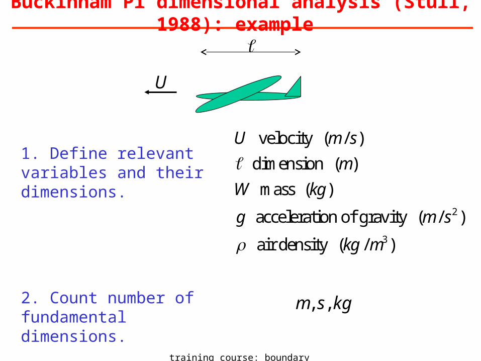
Buckinham Pi dimensional analysis (Stull, 1988): example
U
2. Count number of fundamental dimensions.
kgsm ,,
2
3
velocity ( / )
dimension ( )
mass ( )
acceleration of gravity ( / )
air density ( / )
U m s
m
W kg
g m s
kg m
1. Define relevant variables and their dimensions.

training course: boundary layer II
Buckinham Pi dimensional analysis: example
3. Form n dimensionless groupswhere n is the number of variables minus the number of fundamental dimensions.
235 nn ,..1
221 U
Wg
gravitational force
lift force 32 W
mass of airplane
mass of displaced air
4. Measure as a function of 1 2
5. Further simplification; assume: 3
2 1~ constant constantW i.e.
63/2222 ~~~ UWWUUW

training course: boundary layer II
Weight as a function of cruising speed ( “The simple science of flight” by Tennekes, 1997, MIT press)
106
10-6
Wei
ght (
New
tons
)
Flying objects range from small insects to Boeing 747
W~U6
Speed (m/s)
The great flight diagram

training course: boundary layer II
Dimensional analysis example: windmill/anemometer
1. Define relevant variables and their dimensions.
)(
)(
)(
)(
)/(
3
1
22
mkgdensityair
sspeedangular
smkgmNtorqueT
mdiameterD
smvelocityU
DU
kgsm ,,2. Count number of fundamental dimensions.

training course: boundary layer II
Dimensional analysis example: windmill/anemometer
3. Form n dimensionless groupswhere n is the number of variables minus the number of fundamental dimensions.
235 nn ,..1
231 DU
T
produced power
wind power U
D2
speed of rotor tip
wind speed
5. For an anemometer:
DU
torqueno
/
constant)(0
2
21
4. Measure as a function of 1 2 by changing load.
training course: boundary layer II
Similarity theory: Outline
• Goals, Buckingham Pi Theorem and examples
• Surface layer (Monin Obukhov) similarity
• Asymptotic behaviour and free convection scaling
• The outer layer

training course: boundary layer II
h
.surf
Flux profile
layersurface0 o
For z/h << 1 flux is approximately equal to surface flux.
Relevant parameters:
)/()''(
)/()''()''(/||
)(
32
222/122
smwg
smwvwu
msizeeddyorheightz
ovv
ooo
Say we are interested in wind shear:
z
U
)( 1s
Surface layer similarity (Monin Obukhov similarity)
Considerations about the nature of the process:• z/zo >> 1• distance to surface determines turbulence length scale• shear scales with surface friction rather than with zo

training course: boundary layer II
MO similarity
Four variables and two basic units result in two dimensionless numbers, e.g.:
2/1)/|(| o
z
z
U
2/3)/|(|
)''(
o
ov
v
zwgand
The standard way of formulating this is by defining:1/ 2
*
3*
(| | / )
( ' ')
o
v
v o
u friction velocity
uL Obukhov length
g w
Resulting in:
*u
z
z
Um
dimensionless shear
Stability parameter
L
z
(von Karman constant) is defined such that 1 for / 0m z L

training course: boundary layer II
Observations of as a function of z/L, with
m4.0
Empirical gradient functions to describe these observations:
0//51
0/)/161( 4/1
LzforLz
LzforLz
m
m
Note that eddy diffusion coefficients and gradient functions are related:
z
UKwu m
''
m
m
zu
K
1
*
then
ifstableunstable
MO gradient functions

training course: boundary layer II
MO-similarity applied to other quantities
)/(*
Lzz
q
q
zh
z
q
**
)''(
u
qwq o
Quantity
z
scaling parameter
**
)''(
u
w o
dimensionlessfunction
)/(*
Lzz
zh
u *u )/(*
Lzfu uu
* )/(
*
Lzf

training course: boundary layer II
Integral profile functions
Dimensionless wind gradient (shear) or temperature gradient functions can be integrated to profile functions:
)/()ln(** Lzz
zuU
z
u
z
Um
omm
with:
omz integration constant (roughness length for momentum)
m wind profile function, related to gradient function:
L
zwithm
,1
Profile functions for temperature and moisture can be obtained in similar way.

training course: boundary layer II
MO wind profile functions applied to observations
Stable Unstable
Limit of stable layer

training course: boundary layer II
Similarity theory: Outline
• Goals, Buckingham Pi Theorem and examples
• Surface layer (Monin Obukhov) similarity
• Asymptotic behaviour and free convection scaling
• The outer layer

training course: boundary layer II
Asymptotic behaviour
Limiting cases can help to constrain functions e.g.:
/ 0 : 1 (defines von Karman constant, )mfor z L
*/ : becomes irrelevantfor z L u
Therefore e.g.:1/3*
*
1/3*
( / ) ( / )( ' ')
( / )( ' ')
h
o
o
zuz L u z L
z w
zuz L
z w
free convection scaling

training course: boundary layer II
Example of free convection scaling

training course: boundary layer II
Similarity theory: Outline
• Goals, Buckingham Pi Theorem and examples
• Surface layer (Monin Obukhov) similarity
• Asymptotic behaviour and free convection scaling
• The outer layer

training course: boundary layer II
Above the surface layer (z/h>0.1)
•Fluxes are not constant but decrease monotonically with height•Boundary layer height h and Coriolis parameter f are additional scales.
Neutral PBL; velocity defect law:
hofinsteadscaledepthBLisfuwhere
f
zuf
u
VV
f
zuf
u
UUV
GU
G
/
),(),(
*
*
*
*
*

training course: boundary layer II
Mixed layerConvective boundary layer (mixed layer scaling):
•Effects of friction can often be neglected.•Profiles well mixed, so gradient functions become less important• w* is important turbulence velocity scale
3/1* })''({ hw
gw ov
v

training course: boundary layer II
Stable boundary layer
Local scaling extension of surface layer scaling, where surface fluxes are replaced by local fluxes, in other words:Surface layer closure applies to outer layer as well
3/ 2(| | / )
( ' ')v
v
local Obukhov lengthg w
)/()/|(| 2/1
zz
z
Um
Z-less scalingfar away from the surface, z should drop:
z
zz
z
Um ~)/(
)/|(| 2/1

training course: boundary layer II
Local scaling
Z-less regime

training course: boundary layer II
scaling regions for the unstable BL
Holstlag and Nieuwstadt, 1986: BLM, 36, 201-209.

training course: boundary layer II
scaling regions for the stable BL
Holstlag and Nieuwstadt, 1986: BLM, 36, 201-209.

training course: boundary layer II
Geostrophic drag law
Match surface layer and outer layer to obtain relation between surface drag and geostrophic wind.
B
u
V
A
zf
u
u
U
G
om
G
*
*
*
)ln(1
drag
ageostrophic angle
Plot A and B as a function of stability parameter.
Wangara data