Trading Mechanism, Ex-post Uncertainty and IPO Underpricing

Moez BennouriRouen Business School

Sonia Falconieri�

Cass Business SchoolDaniel Weaver

Rutgers Business School

January 5, 2012

Abstract

Recent literature shows that IPO underpricing is a¤ected by ex-post uncertainty (Falconieri

et al.) that is by uncertainty surrounding the value of the �rm going public that persists in

the secondary market. In this paper we investigates both theoretically and empirically the link

between ex-post uncertainty and di¤erent methods to open trading in the IPO aftermarket.

Our results show that ex-post uncertainty indeed depends on the speci�c trading platform used

to open trade after the IPO. Speci�cally the model suggests that auction markets, such as the

NYSE or AMEX, are more e¢ cient in resolving ex post-uncertainty as opposed to dealership

markets, such as the NASDAQ. The predictions of the model are then tested on as sample

of US IPOs between 1993 and 1998 by using the proxy for ex-post uncertainty proposed by

Falconieri et al. (2009). Consistently with the predictions of the theoretical model, our �ndings

provide strong evidence that there is a larger level of uncertainty at the beginning of trading on

NASDAQ than on exchange-listed IPOs, such as the NYSE or AMEX. This is in turn associated

with larger levels of underpricing for NASDAQ IPOs. Additionally, we use a natural experiment

resulting from the introduction of the Nasdaq IPO opening cross in 2006 to test the robustness

of our �ndings. The opening cross e¤ectively moved Nasdaq closer to the level of centralization

at NYSE or AMEX and thus allows us test whether such change has resulted, as our model

predicts, in a lower level of ex-post uncertainty and hence underpricing for Nasdaq IPOs. The

results of this additional test provide further support to our theory, thereby con�rming the

superior e¢ ciency of auction markets.

Keywords: underpricing, ex post uncertainty, trading platforms.

�Correspondence to: sonia.falconieri.1@city.ac.uk

1

1 Introduction

Underpricing is a peculiar feature of initial public o¤erings (IPOs). While the traditional literature

views underpricing as a premium for ex-ante uncertainty about the �rm market value (Ritter (1984),

Beatty and Ritter (1986)), more recent papers link underpricing to some kind of uncertainty in the

IPO aftermarket. Ellul and Pagano (2006), for instance, develop and test a model that shows that

underpricing is also a¤ected by uncertainty about the after-market liquidity. They �nd that the less

liquid the after-market is expected to be the larger the IPO underpricing. Chen and Wilhelm (2008)

propose a theoretical model that shows that asymmetric information among IPO participants as

well as uncertainty about the �rm value is not fully resolved in the primary market but persists in

the after-market. However, they do not explicitly investigate the link between residual uncertainty

and IPO underpricing which is instead empirically explored by Falconieri et. al. (2009). Falconieri

et al. label "ex-post uncertainty" this residual uncertainty in the IPO aftermarket and develop

proxies for it. Their �ndings document that higher ex-post uncertainty is re�ected in a higher IPO

underpricing.

If ex-post uncertainty a¤ects IPO underpricing, then the question raises as what determines

ex-post uncertainty. This paper addresses this question by investigating, both theoretically and

empirically, whether di¤erent mechanisms to open trading in the aftermarket have an impact on

the level of ex-post uncertainty and consequently of the IPO underpricing.

In the US, till quite recently, there have traditionally been two alternative methods to open

secondary market trading in equities. In order-driven environments like the NYSE, trading starts

with a call auction where public orders are consolidated. In quote-driven markets like NASDAQ,

the �rst trade is preceded by a period (pre-opening) during which dealers can display the prices

at which they will buy and sell. These quotes however are non-binding and do not necessarily

re�ect information from public orders placed with dealers before the opening. The same processes

are used to open secondary market trading after an IPO. If there is some ex-post uncertainty that

persists in the secondary market, then the intuition suggests that the concentrated supply and

demand structure provided by the call auction method of opening trading on the NYSE and the

AMEX should allow for a quicker resolution of any residual value uncertainty than the fragmented

supply and demand resulting from NASDAQ�s method of opening trading. This would in turn

results in less underpricing and narrower spreads on NYSE/AMEX IPOs than for IPOs that trade

on NASDAQ.1

1While previous papers by Boehmer and Fishe (2000) and Ellis, Michaely, and O�Hara (2000) relate underpricingto market structure, they do not directly examine the relationship between the pricing of IPOs and the openingprocedures in the secondary market.In addition, very little has been done to compare IPOs on the two trading systems. Corwin and Harris (2001) and

2

Our model extends that by Ellul and Pagano (2006) to enable us to compare the two trad-

ing platforms. The key feature of the model is the existence of a double adverse selection e¤ect

determined by the fact that the value of the �rm consists of two signals es1 and es2 which are re-vealed, to some investors, in the primary and secondary market respectively. Hence, es2 capturesthe idea of some residual uncertainty in the secondary market. The aim of the model is to show

that auction markets are superior in in reducing information asymmetry and uncertainty and thus

lead to less underpricing that dealership markets. While dealership markets are modeled as in Ellul

and Pagano, we characterize auction markets as having a specialist who aggregates all the orders

on the market, and, based on these, sets up a bid-ask spread. We then construct a measure of

the ex-post uncertainty as de�ned by the ex-post variance of the signal es2 and show that this ispositively related to the IPO underpricing. Next, we conduct simulations to compare the level of

ex-post uncertainty on the two trading platforms. The results of the simulations clearly suggest

that auction markets are better at resolving the residual uncertainty than dealership markets.

The model�s predictions are then tested on a sample of IPO data between 1993 and 1998. We

�nd strong evidence that indeed ex-post uncertainty and thus underpricing are much lower on

auction markets. We conduct a number of robustness check including looking at a sample of IPOs

between June 2006 and May 2008. On May 30, 2006 in fact Nasdaq introduced a voluntary opening

cross. This method resulted in an increased level of centralization of supply and demand on Nasdaq

thereby making it closer to traditional auction markets such as NYSE and Amex. This represents

a natural experiment on which to test the validity of our theory because based on our hypothesis

we would expect less ex-post uncertainty and thus less underpricing on Nasdaq IPO following the

introduction of the opening cross. We �nd that, after 2006, the underpricing of Nasdaq IPOs is

64% smaller than the underpricing of Nasdaq IPO in the previous sample (14.91% vs 23%) and

this seems the results of a reduced ex-post uncertainty which, in the second part of the sample,

becomes much closer to the level of ex-post uncertainty found for the NYSE/Amex IPOs in the

sample 1993-1998. Overall, these �ndings provide strong support to theory.

The reminder of the paper is organized as follows. Related papers are discussed in the next

section. Section 3, sets up and solves the theoretical model. The sample used for our empirical

analysis in detailed in Section 4 and the results of the analysis are grouped in Section 5. Section 6

develops some robustness checks including testing our hypothesis on IPOs in the period following

the introduction of the opening cross on Nasdaq. The last section concludes.

A­ eck-Graves, Hegde, and Miller (1996) compare the size of underpricing on NYSE and NASDAQ IPOs reachingdi¤erent results. However, neither study controls for industry e¤ects, so that their results may be driven by di¤erencesin the types of �rms on each market.

3

2 Literature Review

In the market microstructure literature several papers have investigated the e¢ ciency of alternative

opening procedures. For instance, Madhavan and Panchapagesan (2000) examine the opening pro-

cedures on the NYSE. They show empirically that specialists signi�cantly facilitate price discovery

because they learn from observing the evolution of the limit order book. In a pure single-price

call auction, the opening price would be the one clearing as many shares as possible. However,

on the NYSE the specialist sets a price, which may be di¤erent than the price that would prevail

in a pure auction market with only public orders. This is because of his obligation to provide

price continuity. As a consequence, the opening price is set to provide minimum variation from

the previous day�s close and is shown to be more e¢ cient than the price resulting from an auction

market without specialists. Cao, Ghysels, and Hatheway, (2000) examine instead the pre-opening

on NASDAQ for existing stocks and �nd that market makers seem to use the pre-opening quotes

to signal each other as to their supply and demand.

Few papers have also tried to compare IPOs on the Nasdaq and NYSE but without reaching

consistent results. Corwin and Harris (2001) examine the initial listing decisions of �rms going

public. Using a sample of IPOs from 1991 to 1996 that either listed on the NYSE or met the

NYSE�s minimum-listing requirements and listed on the NASDAQ National Market, they identify

relevant variables in determining which market a newly public �rm will choose for its secondary

trading. By looking at the results of a Probit model, they conclude that the �rm size is the

most important determining factor. Smaller and riskier �rms list on NASDAQ to avoid the higher

listing fees on the NYSE. However, given the higher level of underpricing on NASDAQ, listing on

NASDAQ could also be a strategic decision of underwriters to increase their compensation.

Corwin and Harris also identify some of the determinants of underpricing. They conclude

that the amount of underpricing is related to the aftermarket standard deviation of return (5

day returns over a 100 day window). However, they do not control for industry e¤ects in their

regressions. Therefore, given that NASDAQ stocks are more typically in industries like genetic

engineering or technology �rms, it is entirely possible that the standard deviation of return used in

their regressions may be a proxy for industry membership. In our analysis, we instead control for

the industry by matching NYSE IPOs to NASDAQ IPOs based on 4 digit SIC (Standard Industry

Classi�cation) code and o¤ering size (in US dollars). We also perform control regressions that

include other variables known to related to the level of underpricing.

A­ eck-Graves, Hegde, Miller, and Reilly (1993) �nd, for a sample of IPOs from 1983 to 1987,

no statistically signi�cant di¤erence in the amount of underpricing for NYSE v. NASDAQ/NMS

issues (4.82% v. 5.56%). This is in contrast with the �ndings of Corwin and Harris who instead

4

document marginally signi�cant di¤erences in the underpricing levels on NYSE v. NASDAQ issues.

Therefore, there is disagreement in the literature as to whether the amount of underpricing di¤ers

across US markets.

Beatty and Ritter (1986) argue that the amount of ex ante uncertainty as to true �rm value

is the main determinant of the level of underpricing in IPOs. They build on Rock (1986) which

interprets underpricing as a premium to uninformed investors for the winner�s curse problem they

face vis-à-vis the informed investors, who observe the true �rm value. Beatty and Ritter further

develop this idea by claiming that more ex ante uncertainty worsens the winner�s curse problem

and, consequently, requires larger underpricing. They test their theory by using as a proxy for ex

ante uncertainty the inverse of the gross proceeds raised in the o¤ering as well as the number of

uses mentioned in the prospectus; Ritter (1984) uses instead the standard deviation of the daily

aftermarket return. Although they (and others) �nd empirical support for their proxy, Jenkinson

and Ljungqvist (1996) point out that using standard deviation of return may be an inadequate

proxy since it may re�ect the relationship between risk and return. In this paper we propose a

more direct measure of ex ante uncertainty, which does not su¤er from the problems associated

with typical risk measures.

Recent papers have investigated the possibility that IPO underpricing be related to the char-

acteristics of the aftermarket trading. Ellul and Pagano (2003) theoretically show that IPO un-

derpricing increases with the bid-ask spread. They interpret the bid-ask spread as a measure for

the uncertainty about the level of liquidity in the aftermarket. They test their theory on a sample

of IPO on the LSE between 1998 and 2000, examining several measures of aftermarket liquidity

uncertainty including the volatility of quoted and e¤ective spread measured over the �rst four weeks

of trading in the aftermarket. Their results provide support to the theory. Our paper di¤ers from

Ellul and Pagano (2003) in two respects: �rstly, we focus on the resolution of residual uncertainty

in the aftermarket and we, thus, construct measures for it that are more precise than the simple

bid-ask spread; secondly, while their model only look at dealership markets, we also model an

auction market and compare the degree of ex-post uncertainty on both.

Finally, in a recent paper Ligon and Liu (2011) explicitly explore the e¤ect of the trading

system on IPO underpricing by studying a natural experiment following the change in the order

handling rules (OHR) for all Nasdaq IPOs mandated by the SEC in 1997. The new OHR required

market makers on the Nasdaq to post all limit orders that are better than a dealer�s quote. Such

change has meant an improvement of the aftermarket liquidity on the Nasdaq and as such the

authors expect to have impacted on the underpricing of IPOs listed on the Nasdaq after 1997.

They indeed document a decrease of the underpricing for cold IPOs after the change of the order

5

handling rule.They attribute this result to the fact that the increased liquidity reduces the need

for underwriter price support in cold IPOs.

3 The Theoretical Model

Our model adapts and extends Ellul and Pagano�s model (2006). We consider an IPO market for

new shares over three periods. The primary market takes place at t = 0. We do not explicitly

model the IPO process. Similarly to Ellul and Pagano (2006) we will assume that underpricing in

our set up is mainly associated to Rock�s winner�s curse e¤ect. At t = 1, shares start trading on

the secondary market.2 Finally, at t = 2; all shares are liquidated.

Similarly to Ellul and Pagano (2006), our model captures the interactions between the primary

and the secondary market resulting from a double adverse selection e¤ect due to the existence of in-

formation asymmetries on both markets. However, the novelty of our model and what distinguishes

us from Ellul and Pagano (2006), is that we explicitely analyze the impact of the market struc-

ture on the information linkages between the primary and the secondary market and ultimately on

IPO.performances.

Consequently, the information technology in our model is as follows: it is commonly known that

the shares�fundamental value is eV = V + es1 + es2 where V is a positive constant representing the

non conditional expected value of new shares and es1 and es2 are independently distributed randomvariables representing signals that will be observed by a fraction of the market participants at t = 0

and t = 1; respectively. Both variables are simple binary signals about the quality of the issuer.

The variable es1 is a private signal observed by a number of informed investors during the IPOprocess. It can take value � or �� with probability 1/2. This signal becomes public before the

opening of the trading on the secondary market. Some uncertainty about the shares�value however

remains in the secondary market and is captured by the signal es2 which can take values �" or "with probability 1/2. Given this information structure, the share value is then equal to V + es1 att = 1 and to V + es1 + es2 at t = 2:

In the primary market , there are M uninformed traders who enter the IPO process using only

the available public information and a group of N informed investors who instead observe the value

of es1: Similarly, at t = 1; when trade opens in the secondary market, each trader has a probabilityQ of becoming informed and learning the signal es2 = �" or es2 = " so with probability 1 � Q no

additional information is learned in which case es2 = 0:3 This second signal captures in our2 In line with our empirical analysis we have in mind the very �rst hours after trading opens.3Like in Ellul and Pagano (2006), we assume that becoming informed in the secondary market is independent from

having purchased shares on the primary market. In other words, an investor that has learnt es1 will not necessarilylearn es2 as well.

6

model the idea that there is some residual uncertainty about the �rm�s value that persists in the

aftermarket and in Section 4 we will construct an exact measure for what we will call hereafter

ex-post uncertainty, following Falconieri et al. (2011).

Adverse selection in the secondary market arises as a consequence of the liquidity needs that

agents may face. Since we are concerned with understanding the link between the market structure

and the residual uncertainty in the aftermarket we model the liquidity needs in a richer way

than in Ellul and Pagano. Speci�cally, we assume that each trader in the secondary market may

become a liquidity seller, and thus be forced to sell the shares bought on the primary market, with

probability z; with probability 1�x he may become a liquidity buyer on the secondary market and

with probability 1 � x � z he will hold his shares until the end of t = 2: This assumption implies

two important di¤erences with respect to Ellul and Pagano (2006): �rstly, in their model liquidity

sellers can only be those investors who have purchased shares in the primary market. We instead

allow those investors to be liquidity buyers as well and this is consistent with empirical evidence

(Ellis, 2006) that document that a relevant fraction of the aftermarkes trades come from investors

who want to build up on the allocations received in the primary market. Secondly, we also allow

for the possibility that an investor does not become a liquidity trader in the secondary market

but simply sticks to his share allocation till t = 2: This way of modelling liquidity needs is more

appropriate to capture the idea that there is residual uncertainty that persists in the secondary

markets whereas the Ellul and Pagano framework is more restrictive and can only look at liquidity

uncertainty because the it is essentially centered on the sell-side of the trades in the aftermarket.

The primary market

The primary market in our set-up is organized à la Rock (1986): The underpricing occurs

because of the winner�s curse e¤ect. When they receive new shares, uninformed agents infer that

informed investors have learned negative information about the shares�value. Anticipating this,

uninformed investors will revise downward their valuation of the new assets.

We further assume that the company sells an exogenous number, S; of shares in the IPO. The

objective of the seller and of the underwriter is to maximize the IPO proceeds given by SP0. Each

investor can buy at most one share. Finally, in order to allow for the winner�s curse story, we

assume that uninformed agents are able to buy the whole quantity of shares, i.e. we assume that

M � S: whereas informed investors cannot, i.e. N < S: Hence, the seller needs to attract bids from

the uninformed investors in order to place all the shares.

The secondary market

The secondary market begins at t = 1: At this stage, all investors learn the signal es1: The pricesdetermined on the secondary market will a¤ect the investors�strategies on the primary markets.

7

The price determination mechanism in the secondary market depends in turn on the speci�c market

structure, i.e. whether it is a dealership or an order-book market. Below we spell out in details the

di¤erences between the two market structures and how these are re�ected on the share prices.

Dealership markets

Our de�nition of the dealership market is similar to Ellul and Pagano (2006). Hence, we assume,

with no loss of generality, that each liquidity trader is matched with one dealer and can place an

order for at most 1 unit of shares. Dealers only observe whether the order is a "buy" or a "sell"

order, but cannot know whether it comes from an informed or a liquidity trader. Thus the bid-ask

spread is set based on their expectations of an order coming from an informed or a liquidity trader

and taking into account that the market is assumed to be perfectly competitive. In other words,

the bid and ask prices, denoted by PDb1 and PDa1 respectively, are given by

PDa1 = E�eV j es1;buy� and PDb1 = E

�eV j es1; sell�Order-book market

Considering an order-book market structure along with the dealership one represents the in-

novative part of the model. The peculiar feature of auction markets, such as the NYSE, is that

all the submitted orders are collected by the specialist who therefore has much more information

about the demand than a dealer on a dealership market. We assume however that the specialist

is in competition with other liquidity providers through the market-order book process, this then

implies that given the set of orders y1; y2; :::; ym the price pre share is then given by the following

PA1 = E�eV j y1; y2; :::; ym�

Note that in this market, informed agents will have an incentive to hide their orders behind

liquidity orders in order not to reveal their information. Consequently, since we know that unin-

formed traders will trade at most one unit, informed traders have no incentive to trade more than

one unit either. Therefore, informed investors have to decide whether to sell or buy one unit or,

alternatively, to maintain their position. As speci�ed above, uninformed agents submit orders for

liquidity reasons whereas informed traders trade on the new piece of information they learn at this

stage. Hence, an informed trader i will sell if and only if he expects to make a pro�t from trading,

i.e. i¤�E�eV js2; PO1 �� PO1 � > 0:

Moving backward to the the IPO stage, an investor will bid for shares on the primary market

only if his expected return in the next period given his trading strategy and his information exceed

the IPO o¤er price PM0 where M = fD;Og is the index for dealership and order-book market,

respectively. Consequently, taking into account that each potential buyer on the primary market

8

will subsequently sell the share on the secondary market with probability z; or he will buy a

new share with probability x or, �nally, he will keep the same allocation in t = 1 and liquidate his

position in t = 2 with the remaining probability 1�z�x; we can write the participation constraint

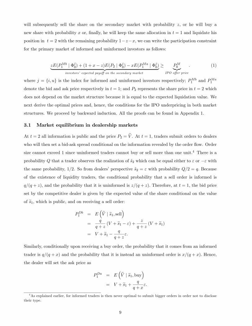
for the primary market of informed and uninformed investors as follows:

zE(PMb1 j �j0) + (1 + x� z)E(P2 j �

j0)� xE(PMa

1 j �j0)| {z }investors� expected payo¤ on the secondary market

� PM0|{z}IPO o¤er price

: (1)

where j = fi; ug is the index for informed and uninformed investors respectively; PMb1 and PMa

1

denote the bid and ask price respectively in t = 1; and P2 represents the share price in t = 2 which

does not depend on the market structure because it is equal to the expected liquidation value. We

next derive the optimal prices and, hence, the conditions for the IPO underpricing in both market

structures. We proceed by backward induction. All the proofs can be found in Appendix 1.

3.1 Market equilibrium in dealership markets

At t = 2 all information is public and the price P2 = eV . At t = 1; traders submit orders to dealerswho will then set a bid-ask spread conditional on the information revealed by the order �ow. Order

size cannot exceed 1 since uninformed traders cannot buy or sell more than one unit.4 There is a

probability Q that a trader observes the realization of ~s2 which can be equal either to " or �" with

the same probability, 1=2. So from dealers�perspective ~s2 = " with probability Q=2 = q: Because

of the existence of liquidity traders, the conditional probability that a sell order is informed is

q=(q + z), and the probability that it is uninformed is z=(q + z): Therefore, at t = 1; the bid price

set by the competitive dealer is given by the expected value of the share conditional on the value

of es1; which is public, and on receiving a sell order:PDb1 = E

�eV j es1; sell�=

q

q + z(V + es1 � ") + z

q + z(V + es1)

= V + es1 � q

q + z":

Similarly, conditionally upon receiving a buy order, the probability that it comes from an informed

trader is q=(q + x) and the probability that it is instead an uninformed order is x=(q + x): Hence,

the dealer will set the ask price as

PDa1 = E�eV j es1;buy�

= V + es1 + q

q + x":

4As explained earlier, for informed traders is then never optimal to submit bigger orders in order not to disclosetheir type.

9

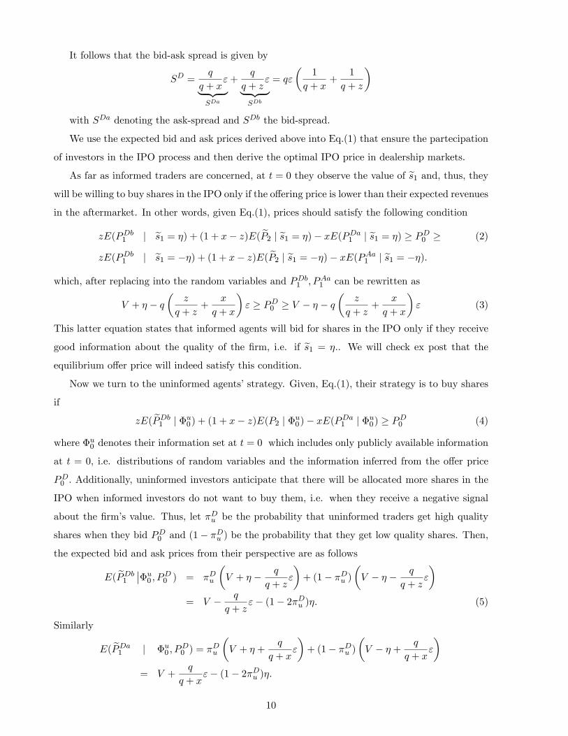
It follows that the bid-ask spread is given by

SD =q

q + x"| {z }

SDa

+q

q + z"| {z }

SDb

= q"

�1

q + x+

1

q + z

�

with SDa denoting the ask-spread and SDb the bid-spread.

We use the expected bid and ask prices derived above into Eq.(1) that ensure the partecipation

of investors in the IPO process and then derive the optimal IPO price in dealership markets.

As far as informed traders are concerned, at t = 0 they observe the value of es1 and, thus, theywill be willing to buy shares in the IPO only if the o¤ering price is lower than their expected revenues

in the aftermarket. In other words, given Eq.(1), prices should satisfy the following condition

zE(PDb1 j es1 = �) + (1 + x� z)E( eP2 j es1 = �)� xE(PDa1 j es1 = �) � PD0 � (2)

zE(PDb1 j es1 = ��) + (1 + x� z)E( eP2 j es1 = ��)� xE(PAa1 j es1 = ��):which, after replacing into the random variables and PDb1 ; PAa1 can be rewritten as

V + � � q�

z

q + z+

x

q + x

�" � PD0 � V � � � q

�z

q + z+

x

q + x

�" (3)

This latter equation states that informed agents will bid for shares in the IPO only if they receive

good information about the quality of the �rm, i.e. if es1 = �:. We will check ex post that the

equilibrium o¤er price will indeed satisfy this condition.

Now we turn to the uninformed agents�strategy. Given, Eq.(1), their strategy is to buy shares

if

zE( ePDb1 j �u0) + (1 + x� z)E(P2 j �u0)� xE(PDa1 j �u0) � PD0 (4)

where �u0 denotes their information set at t = 0 which includes only publicly available information

at t = 0, i.e. distributions of random variables and the information inferred from the o¤er price

PD0 : Additionally, uninformed investors anticipate that there will be allocated more shares in the

IPO when informed investors do not want to buy them, i.e. when they receive a negative signal

about the �rm�s value. Thus, let �Du be the probability that uninformed traders get high quality

shares when they bid PD0 and (1� �Du ) be the probability that they get low quality shares. Then,

the expected bid and ask prices from their perspective are as follows

E( ePDb1 ���u0 ; PD0 ) = �Du

�V + � � q

q + z"

�+ (1� �Du )

�V � � � q

q + z"

�= V � q

q + z"� (1� 2�Du )�: (5)

Similarly

E( ePDa1 j �u0 ; PD0 ) = �

Du

�V + � +

q

q + x"

�+ (1� �Du )

�V � � + q

q + x"

�= V +

q

q + x"� (1� 2�Du )�:

10

E(P2j�u0 ; PD0 ) = �Du (V + �) + (1� �Du ) (V � �)

= V � (1� 2�Du )�: (6)

Substitution into Eq.(4) �nally gives the condition that ensure the uninformed investors�partici-

pation on the primary market:

V � (1� 2�Du )� � q�

z

q + z+

x

q + x

�" � PD0 : (7)

As in Rock (1986); the equilibrium price on the primary market is dictated by the above constraint.

Because N < S; the company will set the highest price PD0 that satis�es the uninformed investors�

participation constraint in the IPO process in order to ensure that all the shares are placed. That

is, PD0 is choses so that the above constraint holds as an equality in equilibrium,

PD0 = V � (1� 2�Du )� � q�

z

q + z+

x

q + x

�" (8)

In the next Proposition we state the next result about the size of underpricing in dealership markets:

Proposition 1 In dealership markets, the level of underpricing is given by

E( ePD1 )� PD0 = (1� �1 + �

)� + q"

�z

q + z+

x

q + x

�(9)

where q"�

zq+z +

xq+x

�measures the ex-post uncertainty on the secondary market.

The above result suggests that IPO underpricing consists of two main components. The �rst

one (1��1+� )� is related to the uncertainty on the primary market consistently with the traditional

explanation of underpricing as a risk premium for the ex-ante uncertainty about the �rm value

(Ritter, 1984; Beatty and Ritter, 1986). The second component q�

zq+z +

xq+x

�" is the one of

interest for us as it captures the ex-post (value) uncertainty, that is the residual uncertainty on the

secondary market after trading starts. As we will show in the next section, the di¤erence in the

size of the underpricing between the markets is only driven by this second component. Also, note

that the formula 9 can be rewritten in term of the bid and ask spreads:

E( ePD1 )� PD0 = (1� �1 + �

)� +�zSDA + xS

DB

�this shows that the underpricing is increasing in the bid and in the ask spread which in a way

represent itself a measure of the ex-post uncertainty as it increases with ": Notice, also, that

contrary to Ellul and Pagano (2006) where the IPO underpricing is solely determined by the sell

side of the secondary market trading, in our model IPO underpricing is also a¤ected by the buy side

of the secondary market trading. The reason for this lies in the richer trading strategies available

11

to investors in our model. Finally, it is important to point out that if the probability of informed

trading q = 0 the second component of the underpricing goes to zero and underpricing will solely be

determined by the uncertainty on the primary market. This is because in the absence of informed

trading on the secondary market there is no further information that can be extracted. Conversely,

ex-post uncertainty is exacerbated by higher uncertainty on liquidity trading, that is by larger x

and z: Again, this is intuitive because the higher the probability of noise trading the more di¢ cult

to disentangle it from informed trading.

3.2 Market equilibrium in order-book markets

As for dealership markets, at t = 2 all information is public and the price P2 = eV . To keep thingstractable, we make the simplifying assumption that in t = 1; there is at most one informed trader

and one liquidity trader who, as before, trades depending on the shock received at t = 1: As before,

then, uninformed agents trade because of liquidity reasons whereas informed agents trade if their

expected pro�ts conditional on their information and the information transmitted by the market

price is strictly positive. For the same reasons explained earlier, it is never optimal for the informed

trader to trade more than one share.

The speci�c feature that distinguish an auction market from a dealership market is the existence

of a specialist who collects all the order and is thus able to observe the aggregate demand denoted by

A = f�2;�1; 0; 1; 2g: Consequently, the specialist is able to extract more information than a dealer

on a dealership market who only knows the order submitted to him, and in some circumstances he

can e¤ectively infer all the information available to the informed investor.

The table below describe in details of all the possible vectors of orders depending on the trading

strategies of the liquidity and informed traders along with the relative probabilities of each of these

vectors. Sell orders have a negative sign and buy orders a positive sign, whereas 0 denotes "no

order". :

Informed order Liquidity trader Total demand Probability Expected alue-1 -1 -2 qz V + es1 � "-1 +1 0 qx V + es1 � "-1 0 -1 q(1� x� z) V + es1 � "0 -1 -1 (1� 2q)z V + es10 +1 +1 (1� 2q)x V + es10 0 0 (1� 2q)(1� x� z) � -1 -1 0 qz V + es1 + "1 +1 +2 qx V + es1 + "1 0 +1 q(1� x� z) V + es1 + "

In this environment, the specialist will set a price PO1 (A) = E�eV jes1; A� for each possible value

of A conditional on the available information as well as the information revealed by the orders

12

submitted by the investors. Before that, we introduce the following piece of notation: let �A be

the probability of having an aggregate order equal to A; then we have

��2 = Pr(A = �2) = qz (10)

��1 = Pr(A = �1) = q(1� x� z) + (1� 2q)z (11)

�0 = Pr(A = 0) = q (x+ z) + (1� 2q)(1� x� z) (12)

�1 = Pr(A = 1) = q(1� x� z) + (1� 2q)x (13)

�2 = Pr(A = 2) = qx (14)

Given the above probabilities, we can now de�ne the market prices for each possible vector of

orders.

When A = �2; the specialist can infer the informed investor�s information, speci�cally that

they have received a negative signal. The price will thus re�ect such information

PO1 (�2) = E�eV j es1;�2� = V + es1 � "

Symmetrically, when A = 2; the specialist infers that the informed investor has received a positive

signal, and hence sets the price equal to

PO1 (2) = E�eV j es1; 2� = V + es1 + ":

If instead, the specialist observes an excess o¤er of one unit, i.e., A = �1; the information is not

fully revealed. The market maker knows that this level of demand may be the result of di¤erent

orders�combination. and he will then factor this into his calculation of the price that will be given

by

PO1 (�1) = E�eV j es1;�1�

=q(1� x� z)

��1(V + es1 � ") + (1� 2q)z

��1(V + es1)

= V + es1 � �q(1� x� z)��1

�"

And symmetrically, for A = 1 we get the following price

PO1 (1) = E�eV j es1; 1�

=q(1� x� z)

��1(V + es1 + ") + (1� 2q)x

��1(V + es1)

= V + es1 + �q(1� x� z)�1

�"

13

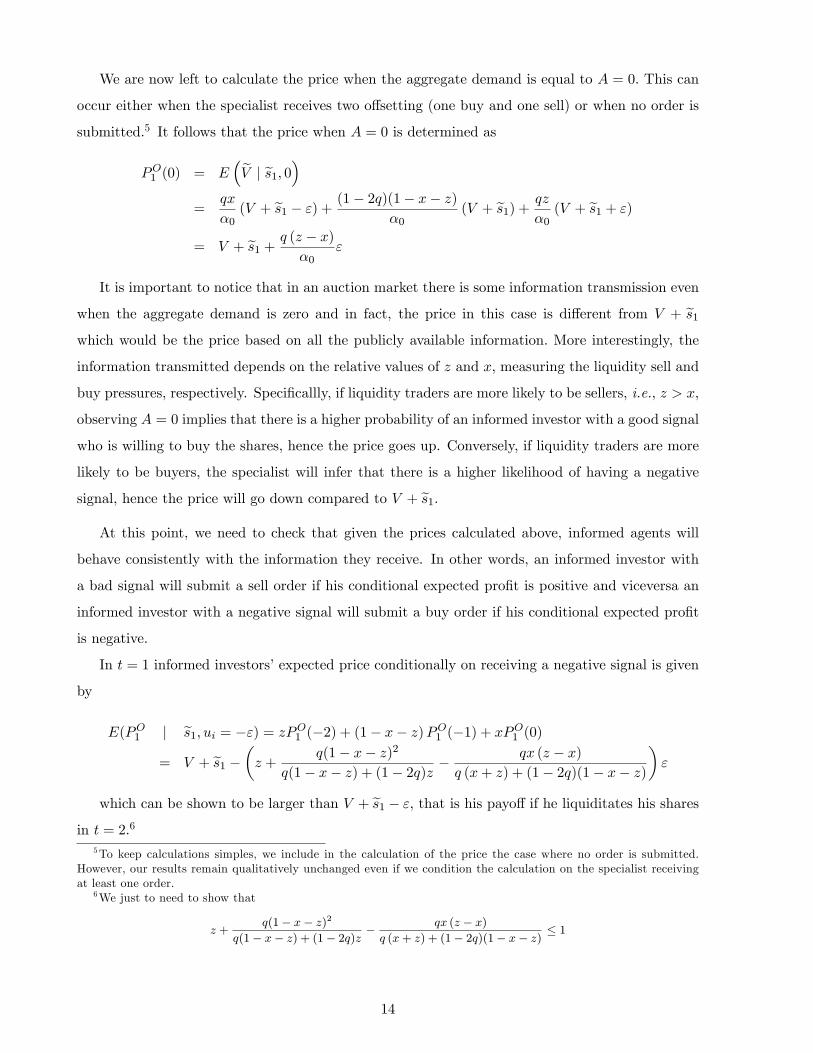
We are now left to calculate the price when the aggregate demand is equal to A = 0: This can

occur either when the specialist receives two o¤setting (one buy and one sell) or when no order is

submitted.5 It follows that the price when A = 0 is determined as

PO1 (0) = E�eV j es1; 0�

=qx

�0(V + es1 � ") + (1� 2q)(1� x� z)

�0(V + es1) + qz

�0(V + es1 + ")

= V + es1 + q (z � x)�0

"

It is important to notice that in an auction market there is some information transmission even

when the aggregate demand is zero and in fact, the price in this case is di¤erent from V + es1which would be the price based on all the publicly available information: More interestingly, the

information transmitted depends on the relative values of z and x; measuring the liquidity sell and

buy pressures, respectively. Speci�callly, if liquidity traders are more likely to be sellers, i.e., z > x;

observing A = 0 implies that there is a higher probability of an informed investor with a good signal

who is willing to buy the shares, hence the price goes up. Conversely, if liquidity traders are more

likely to be buyers, the specialist will infer that there is a higher likelihood of having a negative

signal, hence the price will go down compared to V + es1.At this point, we need to check that given the prices calculated above, informed agents will

behave consistently with the information they receive. In other words, an informed investor with

a bad signal will submit a sell order if his conditional expected pro�t is positive and viceversa an

informed investor with a negative signal will submit a buy order if his conditional expected pro�t

is negative.

In t = 1 informed investors�expected price conditionally on receiving a negative signal is given

by

E(PO1 j es1; ui = �") = zPO1 (�2) + (1� x� z)PO1 (�1) + xPO1 (0)= V + es1 � �z + q(1� x� z)2

q(1� x� z) + (1� 2q)z �qx (z � x)

q (x+ z) + (1� 2q)(1� x� z)

�"

which can be shown to be larger than V + es1 � ", that is his payo¤ if he liquiditates his sharesin t = 2:6

5To keep calculations simples, we include in the calculation of the price the case where no order is submitted.However, our results remain qualitatively unchanged even if we condition the calculation on the specialist receivingat least one order.

6We just to need to show that

z +q(1� x� z)2

q(1� x� z) + (1� 2q)z �qx (z � x)

q (x+ z) + (1� 2q)(1� x� z) � 1

14

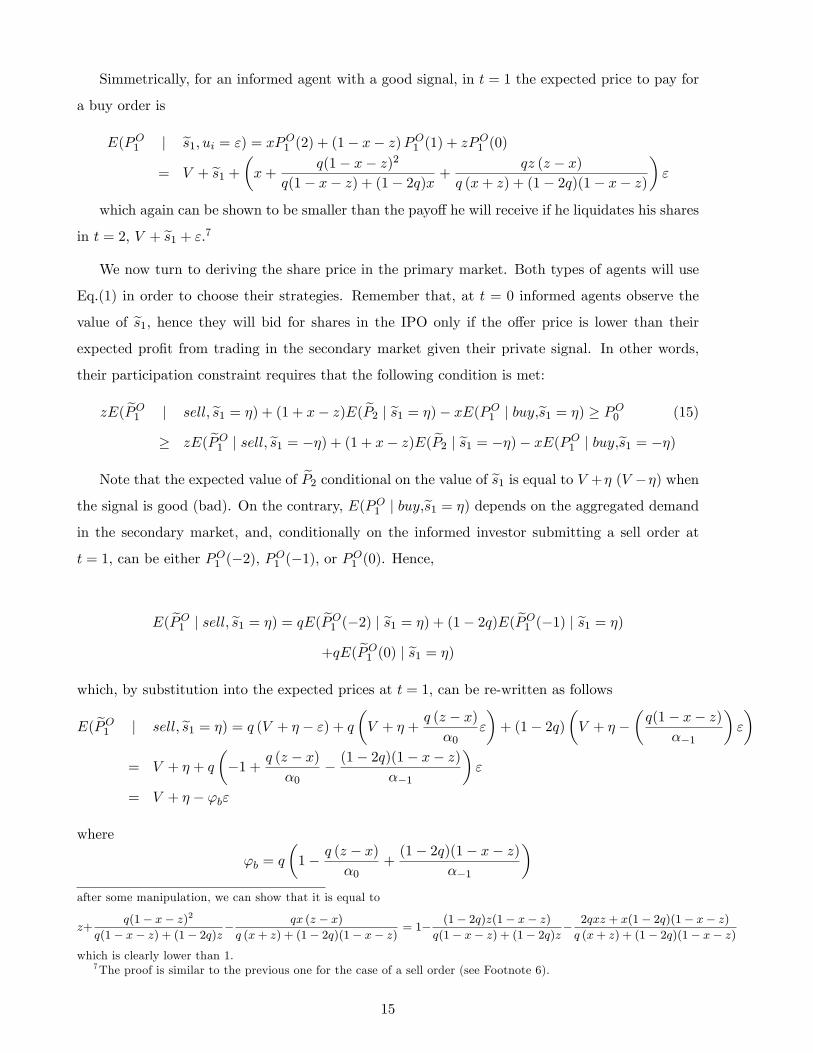
Simmetrically, for an informed agent with a good signal, in t = 1 the expected price to pay for

a buy order is

E(PO1 j es1; ui = ") = xPO1 (2) + (1� x� z)PO1 (1) + zPO1 (0)= V + es1 + �x+ q(1� x� z)2

q(1� x� z) + (1� 2q)x +qz (z � x)

q (x+ z) + (1� 2q)(1� x� z)

�"

which again can be shown to be smaller than the payo¤ he will receive if he liquidates his shares

in t = 2; V + es1 + ":7We now turn to deriving the share price in the primary market. Both types of agents will use

Eq.(1) in order to choose their strategies. Remember that, at t = 0 informed agents observe the

value of es1; hence they will bid for shares in the IPO only if the o¤er price is lower than their

expected pro�t from trading in the secondary market given their private signal. In other words,

their participation constraint requires that the following condition is met:

zE( ePO1 j sell; es1 = �) + (1 + x� z)E( eP2 j es1 = �)� xE(PO1 j buy,es1 = �) � PO0 (15)

� zE( ePO1 j sell; es1 = ��) + (1 + x� z)E( eP2 j es1 = ��)� xE(PO1 j buy,es1 = ��)Note that the expected value of eP2 conditional on the value of es1 is equal to V +� (V ��) when

the signal is good (bad). On the contrary, E(PO1 j buy,es1 = �) depends on the aggregated demandin the secondary market, and, conditionally on the informed investor submitting a sell order at

t = 1; can be either PO1 (�2); PO1 (�1), or PO1 (0). Hence,

E( ePO1 j sell; es1 = �) = qE( ePO1 (�2) j es1 = �) + (1� 2q)E( ePO1 (�1) j es1 = �)+qE( ePO1 (0) j es1 = �)

which, by substitution into the expected prices at t = 1; can be re-written as follows

E( ePO1 j sell; es1 = �) = q (V + � � ") + q�V + � + q (z � x)�0

"

�+ (1� 2q)

�V + � �

�q(1� x� z)

��1

�"

�= V + � + q

��1 + q (z � x)

�0� (1� 2q)(1� x� z)

��1

�"

= V + � � 'b"

where

'b = q

�1� q (z � x)

�0+(1� 2q)(1� x� z)

��1

�after some manipulation, we can show that it is equal to

z+q(1� x� z)2

q(1� x� z) + (1� 2q)z�qx (z � x)

q (x+ z) + (1� 2q)(1� x� z) = 1�(1� 2q)z(1� x� z)

q(1� x� z) + (1� 2q)z�2qxz + x(1� 2q)(1� x� z)q (x+ z) + (1� 2q)(1� x� z)

which is clearly lower than 1.7The proof is similar to the previous one for the case of a sell order (see Footnote 6).

15

Similarily, the expected price conditional on a buy order is given by

E( ePO1 j buy; es1 = �) = qE( ePO1 (2) j es1 = �) + (1� 2q)E( ePO1 (1) j es1 = �)+qE( ePO1 (0) j es1 = �)

= q (V + � + ") + (1� 2q)�V + � +

�q(1� x� z)

�1

�"

�+ q

�V + � +

q (z � x)�0

"

�= V + � + 'a"

where

'a = q

�1 +

(1� 2q)(1� x� z)�1

+q (z � x)�0

�8

By replacing into 15 it is easy to check that the informed agents� participation contraint is

satis�ed.

As in the case of dealership market, we also have to ensure that at t = 0 the uninformed

investors�participation constraint is satistied. That is,

zE( ePO1 j sell;�u0) + (1 + x� z)E( eP2 j �u0)� xE(PO1 j buy,�u0) � PO0 (16)

where �u0 contains all public information available at t = 0, which includes the distributions of

all random variables as well as the information inferred from the o¤er price PO0 : Also, uninformed

investors anticipate that they will be allocated all the shares when informed investors do not bid

for them because they have received a negative signal and they will take this into account when

deciding to participate to the IPO or not. So, let �Ou be the probability that, at the o¤er price PO0 ;

uninformed traders get shares of a high quality �rm (es1 = �) and (1� �Ou ) be the probability thatthey get shares of a low quality �rm (es1 = ��). Consequently, at t = 1 the expected prices fromthe perspective of uninformed investors are de�ned as follows

E( ePO1 ��sell;�u0 ; PO0 ) = �Ou

�E( ePO1 jsell; es1 = � )�+ (1� �Ou )�E( ePO1 jsell; es1 = �� )�

= �Ou (V + � � 'b") + (1� �Ou ) (V � � � 'b")

= (V � 'b")� (1� 2�Ou )�

and

E( ePO1 ��buy;�u0 ; PO0 ) = �Ou

�E( ePO1 jbuy; es1 = � )�+ (1� �Ou )�E( ePO1 jbuy; es1 = �� )�

= �Ou (V + � + 'a") + (1� �Ou ) (V � � + 'a")

= (V + 'a")� (1� 2�Ou )�8The indeces used stand for bid and ask respectively.

16

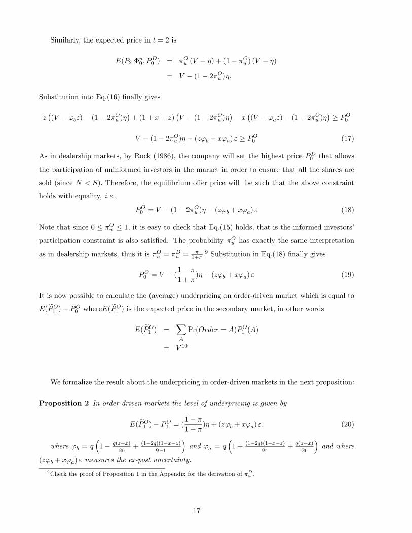
Similarly, the expected price in t = 2 is

E(P2j�u0 ; PD0 ) = �Ou (V + �) + (1� �Ou ) (V � �)

= V � (1� 2�Ou )�:

Substitution into Eq.(16) �nally gives

z�(V � 'b")� (1� 2�Ou )�

�+ (1 + x� z)

�V � (1� 2�Ou )�

�� x

�(V + 'a")� (1� 2�Ou )�

�� PO0

V � (1� 2�Ou )� � (z'b + x'a) " � PO0 (17)

As in dealership markets, by Rock (1986); the company will set the highest price PD0 that allows

the participation of uninformed investors in the market in order to ensure that all the shares are

sold (since N < S): Therefore, the equilibrium o¤er price will be such that the above constraint

holds with equality, i.e.,

PO0 = V � (1� 2�Ou )� � (z'b + x'a) " (18)

Note that since 0 � �Ou � 1; it is easy to check that Eq.(15) holds, that is the informed investors�

participation constraint is also satis�ed. The probability �Ou has exactly the same interpretation

as in dealership markets, thus it is �Ou = �Du =

�1+� :

9 Substitution in Eq.(18) �nally gives

PO0 = V � (1� �1 + �

)� � (z'b + x'a) " (19)

It is now possible to calculate the (average) underpricing on order-driven market which is equal to

E( ePO1 )� PO0 whereE( ePO1 ) is the expected price in the secondary market, in other wordsE( ePO1 ) =

XA

Pr(Order = A)PO1 (A)

= V 10

We formalize the result about the underpricing in order-driven markets in the next proposition:

Proposition 2 In order driven markets the level of underpricing is given by

E( ePO1 )� PO0 = (1� �1 + �)� + (z'b + x'a) ": (20)

where 'b = q�1� q(z�x)

�0+ (1�2q)(1�x�z)

��1

�and 'a = q

�1 + (1�2q)(1�x�z)

�1+ q(z�x)

�0

�and where

(z'b + x'a) " measures the ex-post uncertainty.

9Check the proof of Proposition 1 in the Appendix for the derivation of �Du :

17

Interestingly, the previous result shows that underpricing on auction markets has the same

structure as in the dealership market, as such we can identify and distinguish the e¤ect on under-

pricing due to the uncertainty on the primary market (1��1+� )� which is identical in the two markets;

and the e¤ect on underpricing due to the ex-post uncertainty on the secondary market, captured by

the second term (z'b + x'a) ". We are then able to establish a very important result: �rstly, if the

primary mechanism is the same, di¤erences in the level of underpricing between the two markets

are exclusively driven by the speci�c characteristics of the two trading platforms; secondly, these

speci�c characteristics result in a di¤erent level of ex-post uncertainty on the secondary market.

Ultimately, underpricing will be lower on those markets where the trading structure is more e¤ective

at reducing the ex-post uncertainty. We formalize the previous discussion in the next result.

Proposition 3 The underpricing in order-driven markets is lower than the underpricing in deal-

ership markets if and only if the the ex-post uncertainty on order-driven markets is smaller than

that on dealership markets. That is, if and only if the following condition holds:

z'b + x'a � q�

z

q + z+

x

q + x

�The comparison between the level of ex-post uncertainty cannot be done analitcally, therefore

we need to use simulations to check whether the inequality below holds and under which conditions.

We summarize the results of the simulations in Section 5 whereas in the next section we provide

an alternative way of measuring the ex-post uncertainty which is more in line with the empirical

proxy used in our empirical analysis, that is the standard deviation of the quote mid-points.

4 Ex post uncertainty

In our model, the residual uncertainty on the secondary market is linked to the signal es2 essentially.Consequently, an intuitive measure of the ex-post uncertainty that captures the risk embedded in

the fact that there is more and new information about the �rm value that is processed by the

secondary market is the ex post variance of the signal es2: This is because once the orders arereceived, the market makers on both markets can update their information about the share value

and hence about es2:4.1 Ex post variance in dealership markets

From a dealers�s perspective, the posterior distribution of es2; when order start arriving is given byesp2 = "; 0; �" with probability q; (1 � 2q); q; respectively. The ex-post uncertainty prior to the

opening of the aftermarket trading is then equal to the unconditional variance of es2; 2q"2: Once18

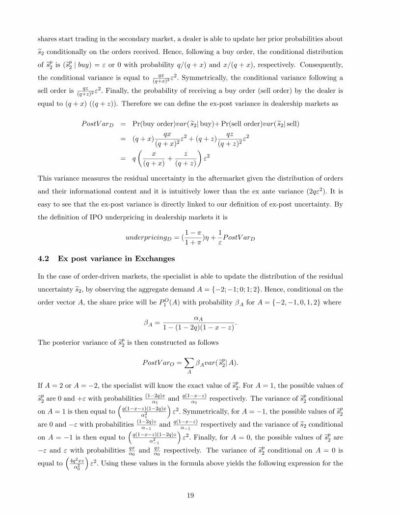
shares start trading in the secondary market, a dealer is able to update her prior probabilities aboutes2 conditionally on the orders received: Hence, following a buy order, the conditional distributionof esp2 is (esp2 j buy) = " or 0 with probability q=(q + x) and x=(q + x); respectively. Consequently,

the conditional variance is equal to qx(q+x)2

"2: Symmetrically, the conditional variance following a

sell order is qz(q+z)2

"2: Finally, the probability of receiving a buy order (sell order) by the dealer is

equal to (q + x) ((q + z)). Therefore we can de�ne the ex-post variance in dealership markets as

PostV arD = Pr(buy order)var(es2jbuy)+Pr(sell order)var(es2j sell)= (q + x)

qx

(q + x)2"2 + (q + z)

qz

(q + z)2"2

= q

�x

(q + x)+

z

(q + z)

�"2

This variance measures the residual uncertainty in the aftermarket given the distribution of orders

and their informational content and it is intuitively lower than the ex ante variance (2q"2): It is

easy to see that the ex-post variance is directly linked to our de�nition of ex-post uncertainty. By

the de�nition of IPO underpricing in dealership markets it is

underpricingD = (1� �1 + �

)� +1

"PostV arD

4.2 Ex post variance in Exchanges

In the case of order-driven markets, the specialist is able to update the distribution of the residual

uncertainty es2, by observing the aggregate demand A = f�2;�1; 0; 1; 2g: Hence, conditional on theorder vector A; the share price will be PO1 (A) with probability �A for A = f�2;�1; 0; 1; 2g where

�A =�A

1� (1� 2q)(1� x� z) :

The posterior variance of esp2 is then constructed as followsPostV arO =

XA

�Avar(esp2jA).If A = 2 or A = �2; the specialist will know the exact value of esp2: For A = 1; the possible values ofesp2 are 0 and +" with probabilities (1�2q)x�1

and q(1�x�z)�1

respectively. The variance of esp2 conditionalon A = 1 is then equal to

�q(1�x�z)(1�2q)x

�21

�"2: Symmetrically, for A = �1; the possible values of esp2

are 0 and �" with probabilities (1�2q)z��1and q(1�x�z)

��1respectively and the variance of es2 conditional

on A = �1 is then equal to�q(1�x�z)(1�2q)z

�2�1

�"2: Finally, for A = 0; the possible values of esp2 are

�" and " with probabilities qx�0and qz

�0respectively. The variance of esp2 conditional on A = 0 is

equal to�4q2xz�20

�"2: Using these values in the formula above yields the following expression for the

19

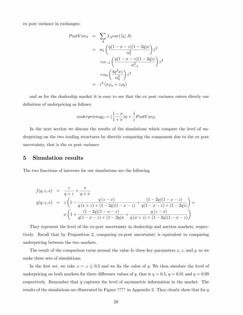
ex post variance in exchanges:

PostV arO =XA

�Avar(es2jA)= �1

�q(1� x� z)(1� 2q)x

�21

�"2

+��1

�q(1� x� z)(1� 2q)z

�2�1

�"2

+�0

�4q2xz

�20

�"2

= "2 (x'a + z'b)

and as for the dealership market it is easy to see that the ex post variance enters direcly our

de�nition of underpricing as follows:

underpricingO = (1� �1 + �

)� +1

"PostV arO

In the next section we discuss the results of the simulations which compare the level of un-

derpricing on the two trading structures by directly comparing the component due to the ex post

uncertainty, that is the ex post variance.

5 Simulation results

The two functions of interests for our simulations are the following

f(q; z; x) =z

q + z+

x

q + x

g(q; z; x) = z

�1� q (z � x)

q (x+ z) + (1� 2q)(1� x� z) +(1� 2q)(1� x� z)

q(1� x� z) + (1� 2q)z

�+

x

�1 +

(1� 2q)(1� x� z)q(1� x� z) + (1� 2q)x +

q (z � x)q (x+ z) + (1� 2q)(1� x� z)

�They represent the level of the ex-post uncertainty in dealership and auction markets, respec-

tively. Recall that by Proposition 2, comparing ex-post uncertainty is equivalent to comparing

underpricing between the two markets.

The result of the comparison turns around the value fo three key parameters x; z; and q so we

make three sets of simulations.

In the �rst set, we take x = z � 0:5 and we �x the value of q: We then simulate the level of

underpricing on both markets for three di¤erence values of q; that is q = 0:5; q = 0:01 and q = 0:99

respectively. Remember that q captures the level of asymmetric information in the market. The

results of the simulations are illustrated by Figure ???? in Appendix 2. They clearly show that for q

20

very small, i.e., when information asymmetry is not important in the market, underpricing in both

markets is very close because the comparative advantage of an auction market is its e¤ectiveness

in reducing the e¤ect of asymmetric information, it asymmetric information is quite small then

such advantage is not relevant. However, as adverse selection problems increase , underpricing in

dealership markets increases more that in auction markets leading to a large i¤erence. Finally,

when q gets very close to 1; the di¤erence shrinks again because the occurrence of informed trading

is nearly certain whilst the occurence of liquidity trading does not create enough noise in the

markets. Note however that when q is very close to 1; underpricing in auction markets presents

several unde�ned values because numerators tend to 0:

In the second set of simulations we �x the value of x and draw the underpricing as functions of

z and q for x = 0:5; 0:01 and 0:99, respectively. We �nd that underpricing in dealership markets

is higher than underpricing on auction markets almost everywhere with this di¤erence becoming

very large as x increases and tends to 1; which can be interpreted as the case of a Hot IPOs where

there would be a strong buying pressure just after the sale.

The last of simulations �xes the value of z and draw the underpricing as a function of x and

q for z = 0:5; 0:01 and 0:99: This set of simulations perfectly replicates the results of the previous

one.

We see thus that for su¢ ciently high level of adverse selection, which we think it is the most

appropriate situation to describe the beginning of trading after an IPO, auction markets clearly

dominate dealership markets.

6 Data

Our �rst step is to compile a list of all IPOs between January 1993 and December 1998 from

the Securities Data Corporation (SDC) New Issues Database. Since we are concerned with the

opening of trading in an IPO, we set the beginning of our sample period to coincide with the

availability of intraday data on the NYSE TAQ database, 1993. We end our sample period in

1998 to avoid in�uences from the NASDAQ technology bubble and its subsequent bursting. Barry

and Jennings (1993) �nd that the returns of operating companies and closed-end-funds behave

very di¤erently. Therefore, consistent with Corwin and Harris (2001), we exclude investment funds

(including mortgage securities), REITs, and real estate �rms from our sample. Also excluded are

ADRs and �rms incorporated outside the United States since they are most likely cross-listed �rms

with established stock values on other exchanges.

We cross-check the o¤ering date and market on both the TAQ and CRSP data bases. CRSP

standard industry classi�cations (SIC) are used for our data rather than SDC�s designation since

21

they are found to be more accurate. Corrections are made to issue dates by con�rming the �rst

trade date on the TAQ data base. Since our hypothesis is that the method of opening trading in

IPOs on exchanges will lead to lower value uncertainty than on NASDAQ, we group NYSE and

AMEX IPOs together for comparison with NASDAQ IPOs. The resulting sample consists of 361

exchange listed stocks and 1,668 NASDAQ stocks.

Table 1 contains descriptive statistics for our sample. Examining Table 1 reveals that the

average exchange-listed IPO is over �ve times larger than the average NASDAQ IPO. Also, the

average exchange-listed IPO o¤ering price is about 5 times larger than the average NASDAQ IPO.

The listing requirements for NYSE stocks are higher than those on the AMEX and NASDAQ.

Therefore, a number of NASDAQ �rms are not eligible for listing on the NYSE and any observed

di¤erences in ex-post value uncertainty (and underpricing) may be due to �rm speci�c di¤erences

and not the method of opening trading. To control for listing choice we create a sub-sample of

NASDAQ stocks that are eligible to list on any exchange at the time of going public. We de�ne

this as any �rm with an o¤ering of at least $40,000,000. There are 444 such NASDAQ �rms.

Examining the last column of Table 1 reveals that these NASDAQ �rms have an o¤ering price

closer to the NYSE/AMEX sample, but that the o¤ering size is still less than half that of the

typical NYSE/AMEX IPO.

7 Empirical Results

The �rst variable we examine is the amount of underpricing for our sample. For this portion of the

study. Consistent with previous studies, we de�ne the amount of underpricing as the o¤er to close

return on the �rst day of trading. The results are contained in Table 1. The amount of underpricing

for NASDAQ IPOs is greater than for NYSE/AMEX IPOs. Overall the average NASDAQ �rst

day return is nearly 80% larger than exchange listed underpricing (9.9% versus 17.7%). The last

column of Table 1 shows that the exchange eligible NASDAQ sub-sample has an even larger (23%)

level of underpricing.

We �nd that NASDAQ �rms are about the same volume of trading as NYSE/AMEX �rms

despite the fact that NYSE/AMEX o¤erings are more than three times as large as the typical

NASDAQ o¤ering (in shares.) Consistent with prior studies, we �nd that NASDAQ �rms are

younger and have higher daily volatility that exchange listed �rms. We next compare spread

patterns for our samples.

22

7.1 Opening and Closing Spreads

Saar (2001) develops a model of demand uncertainty that suggests that a specialist system of

trading (as on the NYSE and AMEX) is better able to ascertain demand (therefore lower demand

uncertainty) and will thus have narrower spreads than a multiple market maker system. Our data

provide a good test of this hypothesis. The results for the opening spreads for IPOs are contained

in Table 1. Opening spreads are de�ned as the spread (ask minus bid) in e¤ect at the time of the

�rst trade or the �rst quote after the �rst trade. NASDAQ spreads are signi�cantly larger than

NYSE/AMEX spreads. In particular, NASDAQ opening spreads are on average two and one half

times larger than exchange listed spreads.

Wide opening spreads are consistent with the uncertain demand hypothesis of Saar (2001).

The fact that we �nd much wider opening spreads on NASDAQ suggests that the method used by

NASDAQ to open trading in IPOs leads to a lower amount of information concerning demand �

vis a vis the opening call auction on exchanges. However, the di¤erence in opening spreads may

merely be a re�ection of the wider spreads on NASDAQ documented by many studies.

McInish and Wood (1992) and Chan, Christie, and Schultz (1995) examine the intraday pattern

of spreads on the NYSE and NASDAQ, respectively. Wood and McInish �nd a reverse J pattern

of spreads for NYSE stocks where closing spreads are about 10% less than opening spreads. Chan,

Christie, and Schultz �nd evidence of a declining spread pattern on NASDAQ stocks with closing

spreads about 5% less than opening spreads. If the di¤erence in opening spreads, between markets,

is due to general market structure rather than to di¤erent levels of demand uncertainty, we would

expect the same di¤erence in closing spreads adjusted by the average intraday decline observed by

other authors. Therefore, we next examine average closing spread on the �rst trading day, for our

sample.

The results, listed just below the results for opening spreads in Table 1, show that the di¤erence

between NYSE/AMEX and NASDAQ closing spreads for underpriced IPOs is less than half of

what it is at the open �$0.15. Comparing closing spreads to opening spreads, for our under-priced

sample, reveals that exchange listed closing spreads are 23% less than opening spreads ($0.16 versus

$0.21), which is consistent with the general pattern for NYSE stocks documented by McInish and

Wood (1992). In contrast NASDAQ closing spreads decline by more than 40% from opening levels.

The NASDAQ decline is far greater than that found in Chan, Christie, and Schultz (1995). This

suggests that the pattern of NASDAQ spreads is di¤erent on IPO days than on other days. It also

provides support for the hypothesis that NASDAQ�s method of opening IPOs is associated with

more uncertainty as to demand than the exchange-listed method.

To complete our analysis of spreads, we return to Figure 1 to examine the intraday spread

23

pattern for our IPO sample to determine how long it takes for the di¤erences in spread width to

reduce. We �nd that while average exchanged-listed spreads (ask minus bid) exhibit an almost

�at pattern over the �rst 10 minutes, the pattern of NASDAQ spreads exhibits a much more

dramatic decline within the �rst 4 minutes of trading. In particular spreads decline by $0.17

in the �rst few minutes. This is in contrast with Chan, Christie, and Schultz (1995) who �nd

spreads are fairly stable on NASDAQ stocks over the �rst 2 hours of trading. The decline in

NASDAQ spreads is consistent with the uncertainty hypothesis suggesting that uncertainty is

resolved within the �rst few minutes of trading. To the extent that underpricing is associated with

ex-post value uncertainty (examined in more depth later) these �ndings suggest that at least part

of the di¤erence in underpricing between stocks in our NASDAQ and exchange-listed samples may

be due to di¤erences in opening procedures.

Four minutes is a slightly more than 1% of the 390 minutes in a full trading day. It could there-

fore be argued that resolving uncertainty in the �rst 4 minutes of trading is of little consequence.

To examine this issue, we calculate the proportion of total �rst day share volume traded in the �rst

4 minutes of trading.

. Examining the percentage of shares traded in the �rst four minutes by listing market type

(Table 1), we �nd that almost 40% of the total daily trading volume in exchange-listed stocks occurs

in the �rst 4 minutes of trading. We further �nd that 15% of NASDAQ �rst day volume occurs

in the �rst 4 minutes. Two observations are warranted. First, it is clear that a large amount of

trading occurs in the �rst few minutes of trading, suggesting that this short time span is important

for a large group of investors. Second the fact that exchanged listed volume in the �rst few minutes

of trading is much greater than NASDAQ volume suggests that it may be related to the greater

uncertainty as to �rm value imparted by that market�s method of opening trading.

7.2 Ex-post Value Uncertainty

Our model shows that some uncertainty about the �rm value persists in the aftermarket and posi-

tively a¤ect the level of underpricing. In order to test this relationship we follow Falconieri, Murphy,

and Weaver (2009) who develop empirical proxies for what they term ex-post value uncertainty.

They show that their proxies greatly improve the explanatory power of previous models of un-

derpricing. The predictions of our theoretical model suggest that the method for opening trading

in an IPO across markets results in higher levels for the ex-post uncertainty measure and hence

underpricing.

Falconieri, Murphy, and Weaver (2009) suggest using the standard deviation of quote midpoints

for the �rst two hours of trading as a proxy for ex-post value uncertainty. They suggest dividing

24

the standard deviation of quote midpoints by the o¤ering price to employ a relative measure.

They also examine the persistence of uncertainty by calculating standard deviations for additional

periods after the initial two hour period. We adopt that methodology here as well. Note that

this empirical proxy is consistent with our theoretical measure of ex-post uncertainty, the ex post

variance of the residual uncertainty. Indeed, an increase of the ex-post variance would increase

the variations of prices and thus it would be re�ected by a higher standard deviation of the quote

mid-point. Furthermore, the standard deviation of the quote mid-point is also able to capture the

e¤ect of an increased trading intensity would also result in a higher standard deviation of the quote

mid-points.

Examining Table 1, we �nd that consistent with our model�s predictions, our NASDAQ sample

exhibits a larger ex-post uncertainty measure than the exchange-listed IPO sample. This suggests

that the fragmented trading structure of the NASDAQ open leads to more value uncertainty as

compared to the more concentrated trading structure of the exchange-listed. The results for the

relative value uncertainty measure exhibits the same pattern. As with the level of underpricing, the

NYSE eligible NASDAQ sample exhibits even stronger di¤erences than the full NASDAQ sample.

Examining the standard deviation of quote midpoints for the remainder of the day as well

as the �rst two hours in the following day, we �nd that for all samples the �rst two hours of

trading appears to have a much higher volatility level, suggesting that a resolution of uncertainty

during that period. Having established that NASDAQ �rms exhibit a higher level of uncertainty

at the beginning of trading, we next examine the relationship of the uncertainty with the observed

di¤erences in underpricing between the di¤erent market types.

7.3 Relationship Between ex-post Value Uncertainty and Under-Pricing

For our next step we investigate whether the amount of underpricing is related to the uncertainty

of demand (as measured by the volatility ratios). Given that we �nd that the larger underpricing

on NASDAQ is as well associated with a higher ex-post value uncertainty proxy as compared to

the exchange-listed, this would suggest the existence of a link between the two variables. We test

for evidence of this relationship.

For each market, we regress the amount of underpricing on our ex-post uncertainty proxy, while

controlling for other variables known to be associated with underpricing, including the o¤ering size

as measured by the IPO proceeds as well as the riskiness of the issue as measured by the volatility

of inter-daily returns over the �rst 20 days of trading. We need to introduce these two controls

because, as we have seen, NASDAQ o¤ering sizes are much smaller than exchange-listed o¤ering

sizes. We need therefore to be sure that the o¤ering size is not the driving force of the di¤erences

25

in the level of underpricing we observe in our sample. Similarly, we need to control for volatility

since residual volatility �after the demand uncertainty is resolved �is higher on NASDAQ than

on the exchange-listed. It may be that the higher underpricing for NASDAQ IPOs is due to their

higher riskiness. Note, that equally priced and over priced IPOs are also included in the sample

for these tests.

We also control for other deal-speci�c characteristics. This includes an indicator of whether

the issue is oversubscribed (hot issues) since there is evidence in the literature (Cornelli and Gol-

dreich (2001)) that oversubscription is positively related to underpricing. We also control for the

reputation of the IPO lead underwriter which the literature documents to be positively related to

the degree of underpricing during our sample period. In addition, we also incorporate �rm speci�c

characteristics such as the age of the �rm and whether the �rm is technology based or a dot com,

which previous studies have shown to be related to underpricing (see Loughran and Ritter (2004)

among others). Consequently, we perform the following regression

%Underi = �+ �1ExPostUncerti + �2Offeringi + �3V olatilityi + �4Hoti + �5Ln(1 + age) + �6Interneti +(21)

�7Techi + �8Ranki

where %Underi is de�ned as (First Day Closing Price � O¤ering Price) / First Day Clos-

ing Price; ExPostUncerti is the standard deviation of spread midpoints for the �rst 2 hours

as constructed by Falconieri et al. (2009); Offeringi is the log of �rm i�s o¤ering size (in mil-

lions of dollars) computed as the total number of shares issued at the o¤ering times the o¤ering

price; V olatilityi is the standard deviation of daily returns. Hoti is de�ned as (O¤ering Price �

Mid Range)/Mid Range; where Mid Range is the midpoint of the originally �led price range11.

Ln(1 + age)is the measure used in Loughran and Ritter (2004) where age is the number of years

since the company was founded.12 Internet and Techare dummy variables assigned the value of

1 if the IPO is an internet or technology IPO, respectively.13 Ranki is the lead underwriter rank

obtained from Loughran and Ritter�s (2004) classi�cation which is based on Carter and Manaster

(1990) and Carter, Dark and Singh (1998) rankings. Underwriters are ranked from 1 to 9 with

higher numbers indicating higher reputation and quality. Regressions are performed both overall

and by market. The results for the absolute measure are contained in Table 2. The results for the

11Cornelli and Goldreich (2002) show that hot issues are more likely to be priced close to the upper bound of theoriginally �led price range.12The source of founding dates is the Field-Ritter dataset of company founding dates, as used in Laura C. Field

and Jonathon Karpo¤ "Takeover Defenses of IPO Firms" in the October 2002 Journal of Finance Vol. 57. No. 5,pp. 1857-1889, and Tim Loughran and Jay R. Ritter, "Why Has IPO Underpricing Changed Over Time?" in theAutumn 2004 Financial Management Vol. 33, No. 3, pp. 5-37.13Both are obtained from Jay Ritter�s website and constitute Appendix C and D of Loughran and Ritter (2004).

26

relative measure are qualitatively similar and hence not reported here.

7.4 Ex-post Uncertainty and Trading Location

Thus far we have observed that our ex-post uncertainty proxy, is directly related to the amount

of underpricing. We also observe that �rms listing on an exchange have lower ex-post uncertainty

proxies than those that trade on NASDAQ. Our model predicts that this is due to the fact that

the consolidated method of opening trading on exchanges leads to lower uncertainty and hence

lower underpricing. To test this prediction, we model our ex-post uncertainty proxy, as a function

of an exchange listing dummy, ExchDum, and a series of control variables. A signi�cant negative

relationship between our ex-post uncertainty proxy and the exchange dummy would support our

conjecture.

First among the control variables is the volatility of daily return, V olatility:We expect a direct

relationship between the ex-post uncertainty proxy and overall volatility. The next control variable

we consider is whether the issue price is signi�cantly higher than the original �ling range. Hot

is de�ned as (O¤ering Price �Mid Range)/Mid Range; where Mid Range is the midpoint of the

original �led price range. The price revisions associated with large values of Hot are indicative of

uncertainty as to the value of the �rm. Therefore we predict a direct relationship.

Note that we would not consider size to be related to our measure of value uncertainty. As proof

of this we call attention to the fact that internet �rms have been among the largest IPOs, yet also

have the most value uncertainty. It is sometimes argued that larger �rms have more information

available about them. This argument seems better applied to the age of the �rm. That is, the

longer a �rm has been in business the more information is available about the operations of the �rm.

This in turn should lead to less uncertainty as evidenced by a smaller volatility ratio. Accordingly,

we include the log of 1 plus the age of the �rm, Ln(1 + age), as a control variable and predict an

inverse relationship between it and our volatility ratio.

By their nature, stocks of technology �rms and internet based �rms may be harder to value

than �rms in more established industries. Internet and Tech are as before dummy variables

assigned the value of 1 if the IPO is an internet or technology IPO, respectively. We expect a

direct relationship between these dummies and our ex-post uncertainty measure. The �nal control

variable we consider is the rank of the lead underwriter. More prestigious underwriters may be

better at determining �rms value than less experienced underwriters. The variable Rank varies

from 1 to 9. Since higher ranked underwriters have larger values of Rank, we predict an inverse

relationship. We model the relationship between our ex-post uncertainty measure and the above

variables as:

27

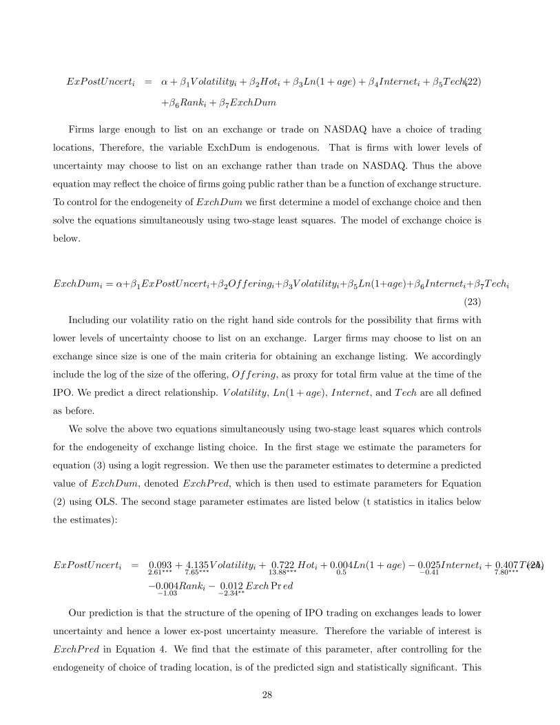
ExPostUncerti = �+ �1V olatilityi + �2Hoti + �3Ln(1 + age) + �4Interneti + �5Techi(22)

+�6Ranki + �7ExchDum

Firms large enough to list on an exchange or trade on NASDAQ have a choice of trading

locations, Therefore, the variable ExchDum is endogenous. That is �rms with lower levels of

uncertainty may choose to list on an exchange rather than trade on NASDAQ. Thus the above

equation may re�ect the choice of �rms going public rather than be a function of exchange structure.

To control for the endogeneity of ExchDum we �rst determine a model of exchange choice and then

solve the equations simultaneously using two-stage least squares. The model of exchange choice is

below.

ExchDumi = �+�1ExPostUncerti+�2Offeringi+�3V olatilityi+�5Ln(1+age)+�6Interneti+�7Techi

(23)

Including our volatility ratio on the right hand side controls for the possibility that �rms with

lower levels of uncertainty choose to list on an exchange. Larger �rms may choose to list on an

exchange since size is one of the main criteria for obtaining an exchange listing. We accordingly

include the log of the size of the o¤ering, Offering, as proxy for total �rm value at the time of the

IPO. We predict a direct relationship. V olatility; Ln(1 + age), Internet, and Tech are all de�ned

as before.

We solve the above two equations simultaneously using two-stage least squares which controls

for the endogeneity of exchange listing choice. In the �rst stage we estimate the parameters for

equation (3) using a logit regression. We then use the parameter estimates to determine a predicted

value of ExchDum, denoted ExchPred, which is then used to estimate parameters for Equation

(2) using OLS. The second stage parameter estimates are listed below (t statistics in italics below

the estimates):

ExPostUncerti = 0:0932:61���

+ 4:1357:65���

V olatilityi + 0:72213:88���

Hoti + 0:0040:5

Ln(1 + age)� 0:025�0:41

Interneti + 0:4077:80���

Techi(24)

�0:004�1:03

Ranki � 0:012�2:34��

ExchPr ed

Our prediction is that the structure of the opening of IPO trading on exchanges leads to lower

uncertainty and hence a lower ex-post uncertainty measure. Therefore the variable of interest is

ExchPred in Equation 4. We �nd that the estimate of this parameter, after controlling for the

endogeneity of choice of trading location, is of the predicted sign and statistically signi�cant. This

28

supports our model�s prediction, that the structure of the opening procedure on exchanges leads

to lower value uncertainty relative to NASDAQ.

To further control for the endogeneity of the ExchDum variable and make sure that our empirical

results are truly due to di¤erent market structures and not instead to a self-selection bias we

partition our NASDAQ sample into those �rms that are large enough to list on the NYSE and

those not large enough. Firms too small to list on the NYSE have no choice but to trade on

NASDAQ, so the distribution of volatility ratio cannot be contaminated by a self-selection bias.

In contrast if �rms can choose between an exchange listing and trading on NASDAQ (and the

observed di¤erences are due to a self selection bias) then larger �rms with less value uncertainty

will choose the NYSE. This self-selection will truncate the distribution of volatility ratios for �rms

that chose to go public on NASDAQ instead of the NYSE.

For our sample of NASDAQ o¤erings, we round ex-post uncertainty measures by 1.00 and

then examine the percentage frequency at each rounded ratio. If our reported di¤erences between

exchanges and NASDAQ are due to a self selection bias, then we would expect the group of �rms

large enough to list on the NYSE to exhibit fewer percentages of �rms with low volatility ratios than

those �rms who cannot list. Figure 2 graphs the percentage frequencies of rounded volatility ratios

for the groups that can list (had a choice) and those that cannot list (had no choice). Examining

Figure 2 reveals remarkably similar patterns. This leads us to conclude that the observed di¤erences

in volatility ratios between exchanges and NASDAQ are not due to a self selection bias.

8 Robustness Tests

8.1 Matched Sample

The �rst robustness check we conduct consists in creating a matched sample of �rms that listed on

each market type and compare variables of interest employing paired-di¤erence t tests. Creating

a matched sample controls for industry e¤ects and market conditions. For each NYSE �rm, we

�nd all NASDAQ �rms with the same Fama-French industry that went public within 12 months

of the NYSE IPO. This latter condition attempts to correct for biases related to overall market

conditions. In the case of multiple NASDAQ matches we choose the NASDAQ IPO that is closest

in value to the NYSE IPO. This results in a �nal sample of 128 NYSE IPOs and a matched sample

of 128 NASDAQ IPOs. Our sample of 256 IPOs is much smaller than the actual number of IPOs

that occurred during our sample period but is similar in size to the 220 IPOs examined in Corwin,

Harris, and Lipson (2004). Our matching methodology allows us to control for overall market

conditions as well as industry e¤ects. Therefore, we are not subject to the criticism that NASDAQ

IPOs have a larger amount of underpricing due to the fact that more technology stocks list there.

29

We thus feel that our design will allow us to draw inferences about the impact of di¤ering market

designs on the level of underpricing.

Notwithstanding the reduction in sample size, we compute the di¤erence for each pair for

variables of interest and compute a paired di¤erence t test. The results are contained in Table 3.

Turning �rst to the di¤erences in o¤ering size, we observe that our matching procedure produced

NASDAQ �rms that are less than one third the size of their NYSE match and are 40% riskier. The

NASDAQ matches, consistent with our full sample results, have wider spreads both at the open

and close on the �rst trading day. Also consistent is the fact that the change in spread over the

course of the �rst trading day is signi�cantly larger for NASDAQ �rms.

The variable of highest interest is our ex-post uncertainty measure. We �nd that the measure

is nearly one third larger for the NASDAQ matches. This supports the idea that di¤erences in

the ex-post uncertainty measure between the market types is not driven by di¤erences in industry

types or market conditions at the time of the IPO.

8.2 The Nasdaq Opening Cross

On May 30, 2006, NASDAQ implemented a voluntary opening cross as a supplement to the process

it uses to open trading in IPOs. Investors can either have their orders submitted as part of the

cross or allow dealers to display their orders in the dealer�s quote. Recall that our hypothesis is

that the centralization of supply and demand in an exchange�s open call method to begin trading

in IPOs contributes to a reduction in the ex-post uncertainty as to IPO value. The NASDAQ

IPO opening cross increases the centralization of supply and demand and therefore should reduce

ex-post uncertainty. It therefore serves as a good test of our hypothesis. If we view the degree of

centralization of supply and demand as a continuum then the NASDAQ IPO Open Cross can be

viewed as moving NASDAQ closer to the level of centralization at the NYSE and AMEX. Thus we

expect that following the implementation of the opening cross that our proxy for ex-post uncertainty

would be smaller than in our earlier sample and that the amount of under pricing would be smaller

on NASDAQ as well.

To test our hypothesis of less ex-post uncertainty on NASDAQ following the start of open cross,

we extract from SDC all IPOS after May 30, 2006. To avoid contagion from the �nancial crisis in

the last half of 2008, we end our sample on May 30, 2008. Following the criteria established in the

data section we end up with 277 IPOs in the opening cross sample. Of those 195 are NASDAQ

IPOs and 82 are NYSE, AMEX, or ARCA IPOs. Examining the microstructure of markets in this

latter sample, we �nd some challenges in determining the opening trade as well as order types. Our

�rst challenge was that in the latter period some stocks had a number of trades prior to the �rst

30

trade on the listing exchange. For example FCSX had 266 trades on ARCA before it began trading

on NASDAQ. Therefore, we set the opening of the stock as the �rst trade on the listing exchange.

The opening quote is then set as the BBO quote occurring at or near the opening trade.14

Regulation National Market System, enacted in 2005 led to the implementation of new order

types which are frequently used in our latter period. For example inter-market sweep and NYSE

DIRECT orders each account for about 15% of the trade condition codes over the �rst two days of

trading in IPOs. These trades are included in our sample of trades.15 To calculate BBNO quotes

we include individual exchange quotes market as opening quotes (condition code 10), closing quotes

(condition code 3), regular one-sided quotes (condition code 99), as well as regular quotes (condition

code 12).

The descriptive statistics for our latter sample are contained in Table 4. Comparing these

results with those in Table 1, we �nd that the IPO o¤ering sizes arev much larger than in the

previous period. Overall the average IPO is $178 million in the latter period, but only $58 million

in the former. We �nd that o¤ering prices are higher as well. Average �rst day share volume is

much larger in the latter period (6.7 million versus 1.4 million shares) which probably re�ects the

advent of high frequency trading noted in other studies. Turning to the percentage of shares traded

in the �rst four minutes we �nd that for NASDAQ �rnms, the percenatge traded in the �rst four

minutes in 150% larger than the former sample. This would be consistent with a quicker resolution

of ex-post uncertainty resulting from the opening cross.

We also �nd that the riskiness of NASDAQ �rms in our sample, as measure by the standard

deviation of daily returns, is fairly close in our latter sample (3.27% versus 3.37%). On average

IPOs are being underwritten by �rms with higher ranking than in our former sample. Turning to

the amount of underpricing (�rst dayb return), we �nd that while in the former period NASDAQ

IPOs were underpriced by almost double that of NYSE/AMEX stocks; in the instant period NAS-

DAQ and other IPOs are underpriced by virtually the same amount. This is consistent with our

hypothesis.

Our hypothesis suggests that this reduction in underpricing is the result of a reduction in ex-

post uncertainty. Our proxy for this is the standard deviation of quote midpoints in the �rst two

hours of trading. Comparing these results with those from Table 1, we �nd that while in the former

period, the average NASDAQ IPO exhibits a higher level of ex-post uncertainty than NYSE/AMEX

IPOs, the ranking is reversed in the latter period. Again this is consistent with our hypothesis.

14we �nd that opening quote sometimes predate the opening trade by 2 seconds.15As an aside, we �nd that trade condition codes M and Q, which are found in the TAQ dataset for our sample,

are not de�ned in the TAQ manual. For these codes we consulted the NASDAQ Trader website and �nd that theymost likely represent the NASDAQ o¢ cial closing and opening prices respectively. These trades are also included inour dataset.

31

In Table 5 we report the results of regressions for the latter period similar to those reported

earlier in Table 2. The variable of interest is the parameter estimate for our ex-post uncertainty

measure. While our hypothesis makes no predictions as to any changes in this variable, it should

still be signi�cant and positive, as it is for both NASDAQ and other IPOs. Of note is the �nding

that the parameter estimate for NYSE/AMEX/ARCA IPOs is an order of magnitude larger than

in the former period (0.258 versus only 0.023). The R2 for the latter period is also nearly 3 times

larger than in the former sample. Over the interval between our sample periods, the percentage of

volume traded o¤-exchange for NYSE stocks increased dramatically from 20% to nearly 80%.

We also �nd that the amount of underpricing and ex-post uncertainty on NYSE stocks increased.

This suggests that the increase in o¤ exchange trading may be related to the observed increase in

ex-post uncertainty on NYSE IPOs.

Below we replicate Regression 4 for our new sample of data.

To control for the self-selection bias discussed earlier, we again perform the two-stage regression

described in Equations 2 and 3 for our NASDAQ Opening Cross sample. Recall that the �rst stage

is to perform a logistic regression to determine the probability that a �rm will list on the NYSE,

AMEX, or ARCA based on its characteristics. In the second stage, we use the predicted value of

ExchDum from the �rst stage in the second stage. As explained earlier, the NASDAQ IPO Opening

Cross is supplemental to their traditional process of market maker quotes. Thus, the opening call

auction process employed by exchanges should still have a lower level of ex-post uncertainty than

NASDAQ�s Opening Cross.

Therefore, we would expect, ceteris paribus, the parameter estimate for ExchPred will be

negative, but smaller than for the earlier sample. Examining the parameter estimate of interest in

Equation 5, we �nd that indeed the parameter estimate for ExchPred is negative and statistically

signi�cantly. However, when compared to the model regressed on pre-Opening Cross data, it is less

than one third the size. That is, after controlling for variables thought to be associated with �rm

speci�c ex-post uncertainty, Exchanges still exhibit lower ex-post uncertainty - but the di¤erences

are much smaller. (isn�t it te opposite?the economic e¤ect is stronger)

9 Conclusion

This paper develops a theoretical model that compares the e¤ect of di¤erent trading platforms

on IPO underpricing. Speci�cally, we look at order-driven market (NYSE, Amex) as opposed to

dealership markets (Nasdaq). Recent papers (Chen and Wilhelm (2006); Falconieri et al. (2009))

show that the uncertainty surrounding newly listed �rms is not completely resolved on the primary

market and in fact moves on to the secondary market. Falconieri et al. (2009) label this type of

32

uncertainty, ex-post uncertainty. They construct proxies for it and show that there is a positive

relationship between the degree of ex-post uncertainty and the level of IPO underpricing.

Building on their results, in this paper we argue and show, both theoretically and empirically,

that the underpricing di¤erentials observed between Nasdaq IPOs and NYSE IPOs might then

be the explained by the di¤erent degree of ex-post uncertainty on the two trading platforms.

Speci�cally, our model shows that a centralized system like the NYSE is more e¢ cient in reducing

ex-post uncertainty as opposed to a more fragmented system like the one used to open trade on

the Nasdaq.

The model�s prediction are tested on a sample of IPOs between January 1993 and December

1998. The empirical analysis supports the model�s prediction and con�rms that the degree of ex-

post uncertainty and consequently the level of underpricing is lower on exchanges than on Nasdaq.

The introduction of the opening cross on the Nasdaq in 2006 which e¤ectively moved Nasdaq

closer to the level of aggregation of demand and supply typical of an exchange represents an excellent

natural experiment to check the robustness of our �ndings. Therefore, we replicate our analysis on

a new sample of IPOs between June 1, 2006 and May 30, 2008. As we would expect, we �nd that

after the implementation of the opening cross, Nasdaq IPOs exhibit a much lower underpricing and

surprisingly closer to the level of underpricing of NYSE and Amex IPOs.

In term of policy recommendation, our �nding suggests that if NASDAQ were to adopt a call

auction to begin trading, as some have suggested, the result would be a lower level of underpricing

for IPOs traded there.

References

References

[1] A­ eck-Graves, J., S. Hegde, and R. E. Miller, 1996, �Conditional Price Trends in the After-

market for Initial Public O¤erings.�Financial Management, 25, 25-40.

[2] A­ eck-Graves, J., S. Hegde, and R. E. Miller, and F. K. Reilly, 1993, �The E¤ect of the

Trading System on the Underpricing of Initial Public O¤erings. �Financial Management, 22,

99-108.

[3] Aggarwal, R. and P. Conroy, 2000, �Price Discovery in Initial Public O¤erings and the Role

of the Lead Underwriter.�Journal of Finance, 55, 2903-2922.

[4] Aggarwal, R., Nagpurnanand R.P. and M. Puri, 2002, �Institutional Allocation in Initial Public

O¤erings: Empirical Evidence.�Journal of Finance, 57, 1421-42

33

[5] Allen, F. and G. Faulhaber, 1989, �Signaling by Underpricing the IPO Market.� Journal of

Financial Economics, 23(2), 303-23.

[6] Barry, C.B. and R.H. Jennings, 1993, �The Opening Price Performance of Initial Public Of-

fering of Common Stock.�Financial Management (Spring), 54-63.

[7] Beatty, R., and J. Ritter, 1986, �Investment Banking, Reputation, and the Underpricing of

Initial Public O¤erings.�Journal of Financial Economics, 15, 213-232.

[8] Boehmer, E., and R. P. H. Fishe, 2000, Do Underwriters Encourage Stock Flipping? A New

Explanation for the Underpricing of IPOs. Working paper, University of Georgia.

[9] Bradley, D. J., and B.D. Jordan, 2002, �Partial Adjustment to Public Information and IPO

Underpricing.�Journal of Financial and Quantitative Analysis, 37, 595-616.

[10] Cao, C. E. Ghysels, and F. Hathaway, 2000, �Price Discovery without Trading: Evidence from

the NASDAQ Preopening.�Journal of Finance, 55, 1339-1365.

[11] Carter, R., Manaster, S., 1990. �Initial public o¤erings and underwriter reputation.�Journal

of Finance, 45, 1045�1068.

[12] Carter, R., F. Dark, and A. Singh, 1998, �Underwriter Reputation, Initial Returns, and the

Long-run Performance of IPO Stocks,�Journal of Finance 53, 285-311.

[13] Chan, K. C., W.C. Christie, and P. H. Schultz, 1995, �Market structure and the intraday

pattern of bid-ask spreads for NASDAQ Securities,�Journal of Business,. 68 35-60.

[14] Cornelli, F. and D. Goldreich, (2002): �Bookbuilding: How Informative is the Order Book?�

Journal of Finance, 58, 1415-1443.

[15] Corwin, S. and J. Harris, 2001, �The Initial Listing Decisions of Firms that Go Public.�

Financial Management, Spring, 35-55.

[16] Corwin, S., J. Harris and M. Lipson, 2004, �The Development of Secondary Market Liquidity

for NYSE-listed IPOs.�Journal of Finance, 59, 2339-73

[17] Ellis, K., R. Michaely, and M. O�Hara, 2000, �When the Underwriter is the Market Maker:

An Examination of Trading in the IPO Aftermarket.�Journal of Finance, 55, 1039-1074.

[18] Ellis, K, 2006, "Who Trades IPOs?A Close Look at the First Days of Trading", Journal of

Financial Economics, 79, 339-63.

34

[19] Ellul, A. and M. Pagano, 2006, �IPO Underpricing and Aftermarket Liquidity.� Review of

Financial Studies, 19, 381-4

[20] Falconieri, S., A. Murphy and D. Weaver, 2009, "Underpricing and Ex-Post Value Uncer-

tainty", 38, 285-300.

[21] Jenkinson, T. and A. Ljungqvist, 1996, Initial Public O¤erings, Oxford Press.

[22] Ligon, J.A. and H. Liu, 2011, "The E¤ect of the Trading System on IPO Underpricing: Evi-

dence from the 1997 Order Handling Rule", Journal of Financial Research, 34, 103-30.

[23] Loughran, T. and J. Ritter, 2004, �Why has IPO underpricing increased overtime?�Financial

Management, 33, 5-37.

[24] McInish, T. H. and R.A. Wood, 1992, �An Analysis of Intraday Patterns in Bid / Ask Spread

for NYSE Stocks,�Journal of Finance, 47 I753-764.

[25] Ritter, J.R., 1984, �The �hot issue�market of 1980.�Journal of Business, 57, 215-40.

[26] Rock, K., 1986, �Why new issues are underpriced.�Journal of Financial Economics, 15, 187-

212..

35

10 Appendix 1: The Proofs

Proof of Proposition 1: Let us start by noticing that given

PD0 = V � (1� 2�Du )� � q�

z

q + z+

x

q + x

�" (25)

and since 0 � �D � 1; it is easy to check that Eq.(3) holds, so the participation constraint by

informed traders is satis�ed by the o¤er price.

By its de�nition, we can rewrite the probability �Du as follows

�Du = Pr (es1 = � j uninformed get shares)taking into account that uninformed investors get shares with probability 1 when the signal is

bad which occurs with probability 1=2 and get shares with probability � =M=(M +N) when the

signal is good which again occurs with probability 1=2; we can then write

�Du =

M2(N+M)

M2(N+M) +

12

=

M(N+M)

M(N+M) + 1

=�

1 + �:

Replacing this into Eq.(8) allows to rewrite the o¤er price as

PD0 = V � (1� �1 + �

)� � q�

z

q + z+

x

q + x

�": (26)

By de�nition, underpricing is measured by the following di¤erence E( ePD1 ) � PD0 where ePD1 is the

expected price in the secondary market at t = 1 and is equal to

E( ePD1 ) = Pr(buy order)E(PDa1 ) + Pr(sell order)E(PDb1 )

where Pr(buy order) = (x + q)=(2q + x + z) and, similarly, Pr(sell order) = (z + q)=(2q + x + z)

which �nally yields that E( ePD1 ) = V . From this, it is then straightforward to derive the level of

undepricing in dealership markets.

11 Appendix 2: SIMULATIONS RESULTS

We de�ne the following functions:

f(q; z; x) =z

q + z+

x

q + x

g(q; z; x) = z

�1� q (z � x)

q (x+ z) + (1� 2q)(1� x� z) +(1� 2q)(1� x� z)

q(1� x� z) + (1� 2q)z

�+

x

�1 +

(1� 2q)(1� x� z)q(1� x� z) + (1� 2q)x +

q (z � x)q (x+ z) + (1� 2q)(1� x� z)

�

36

representing the values of the ex-post uncertainty in dealership and in auction markets, respec-

tively. Because of the complex structure of underpricing in auction markets, we are not able to

compare these two terms analytically. Consequently, we run simulations in order to make these

comparison. Remember that by Proposition 2, comparing ex-post uncertainty is equivalent to

comparing underpricing between the two markets.

We begin by the case where liquidity buying pressure and selling pressure are the same in the

market, i.e., x = z: Figure 11 depicts underpricing in both markets in that case. Clearly, we have

that underpricing is positive for all values of q and z belonging to (0; 0:5) and that underpricing in

dealership markets is larger almost everywhere.

0.1

0.40.5

z

0.3

0.2

1

0 ­1

0.0

0.1

q

0.3

0.5

0.4

0.2

0.0

2

Figure 11: Underpricing in auction and dealership markets when x = z as a function z and q:

Note for Figure 11: Underpricing in auction markets (blue curve) and in dealership markets (green curve) as a

function of the liquidity trading pressure (z) and of information asymmetry (q) where both q and z are between

0 and 0:5:

We simulate underpricing in both markets by �xing each time the variable a¤ecting it in both

markets. By �xing q; Figure , Figure and Figure... depict the way �xing q a¤ects underpricing in

both markets for q = 0:5; a low value of q (0:01) and a large value of q (0:99); respectively.

37

0.0

0.1 0.10

0.0

­1

0.2

0.30.4 xz

0.50.6

0.70.8

0.91.01.0

0.90.8

0.70.6

0.50.4

0.3

0.2

1

2

Underpricing in auction and dealership markets as a function of x and z for a �xed q (q = 0:5)

Note for Figure 11: Underpricing in auction markets (blue curve) and in dealership markets (green curve) as a

function of the liquidity selling pressure (z) and liquidity buying pressure (x) both lying between 0 and 1 and with

the constraint that x+ z � 1 and with a �xed q = 0:5

38

0.60.7

0.5

0.80.9

1.0

0.3

0.4

0

0.2

­1

0.3

0.5

0.70.8

0.6

0.4

0.2

0.10.1

1.00.9

zx

0.0 0.0

1

2

Underpricing in auction and dealership markets as a function of x and z for a �xed q (q = 0:01)

Note for Figure ??: Underpricing in auction markets (blue curve) and in dealership markets (green curve) as a

function of the liquidity selling pressure (z) and liquidity buying pressure (x) both lying between 0 and 1 and with

the constraint that x+ z � 1 and with a �xed q = 0:01

39

0.00

0.00.2

­1

0.2

x

0.4

1.0 0.8 0.6

z0.4

0.60.8

1.0

1

2

Underpricing in auction and dealership markets as a function of x and z for a �xed q (q = 0:99)

Note for Figure 11: Underpricing in auction markets (blue curve) and in dealership markets (green curve) as a

function of the liquidity selling pressure (z) and liquidity buying pressure (x) both lying between 0 and 1 and with

the constraint that x+ z � 1 and with a �xed q = 0:99

Note that for q very small, i.e., when information asymmetry is not important in the market,

underpricing in both markets are very close since our model captures only the asymmetric infor-

mation e¤ect. However, as adverse selection problems increase, underpricing in dealership markets

increases more that in auction markets leading to a higher di¤erence. When q is very close to 1;

the di¤erence shrinks again since informed traders are more likely and the occurence of liquidity

trading does not create enough noise in both markets. Note however that when q is very close

to 1; underpricing in auction markets presents several unde�ned values because numerators can

sometimes be very close to 0:

Figures 11, 11 and 11 depict underpricing as functions of z and q for x = 0:5; 0:01 and 0:99,

respectively. Like in the other cases, underpricing in dealership markets is almost higher almost

everywhere.

40

0.1 0.2 0.3 0.4 0.50.1

z

0.30.5 0.4 0.2

1

­1

00.00.0 q

Underpricing in auction and dealership markets as a function of q and z for a �xed x (x = 0:5)

Note for Figure 11: Underpricing in auction markets (blue curve) and in dealership markets (green curve) as a

function of the liquidity selling pressure (z) is between 0 and 1 � x and information asymmetry (q) lies between

0 and 0:5 and with a �xed x = 0:5

41

0.1

0.2

0.3

0.4

0.5

q

2

1.0

0.0 0.00

0.2

­1

0.4z0.5

0.7

0.90.8

0.6

0.3

0.1

1

Underpricing in auction and dealership markets as a function of q and z for a �xed x (x = 0:01)

Note for Figure 11: Underpricing in auction markets (blue curve) and in dealership markets (green curve) as a

function of the liquidity selling pressure (z) is between 0 and 1 � x and information asymmetry (q) lies between

0 and 0:5 and with a �xed x = 0:01

42

0.1

0.2q

0.40.3

0.52

3

0.000 0.0

­1

0

­2

0.002z

0.006

0.0100.008

0.004

1

Underpricing in auction and dealership markets as a function of q and z for a �xed x (x = 0:99)

Note for Figure 11: Underpricing in auction markets (blue curve) and in dealership markets (green curve) as a

function of the liquidity selling pressure (z) is between 0 and 1 � x and information asymmetry (q) lies between

0 and 0:5 and with a �xed x = 0:99

Note that the last case should be the most representative of hot IPOs since in that case investors

will be incited to buy new shares in the secondary market increasing buying pressure with respect

to selling pressure. In this case the underpricing is larger in dealership markets for all values of q

and z:

Finally, we �x z and simulate underpricing as function of q and x: Results are the same as for

x and are not presented here but are available upon request.

*****************************************************************************************************************************************************

z = 0:5

43

q

0.5 2

­1 0.0 0.5

x0.0

z = 0:01

­2q

0.00.5 z

2 1

x0

g(q; 0:99; x) = 0:99 qq(x+0:99)+(2q�1)(x�0:01) (x� 0:99)�x

�q

q(x+0:99)+(2q�1)(x�0:01) (x� 0:99) + (2q � 1)x�0:01

q(x�0:01)+x(2q�1) � 1��

0:99 (2q � 1) x�0:011: 98q+q(x�0:01)�0:99 + 0:99

44

q

0.5 2

­2 0.000.0x

0.01

f(q; 0:99; x) = 0:99q+0:99 +

xq+x

45