Trading Fees and Efficiency in Limit Order

Markets.∗

Jean-Edouard Colliard

Paris School of Economics

48 boulevard Jourdan

75014 Paris, France

colliard@pse.ens.fr

Thierry Foucault

HEC, Paris

1 rue de la Liberation

78351 Jouy en Josas, France

foucault@hec.fr

October 2011-Under Revision for the Review of Financial Studies.

Abstract

Common wisdom has it that competition between trading platforms in securities

markets benefits investors because it forces platforms to charge smaller fees. We chal-

lenge this view by showing that a decrease in trading fees can impair investors’ expected

welfare in limit order markets. Indeed, a decrease in trading fees can induce investors

to strategically post limit orders with a smaller execution probability, in order to earn

a greater surplus in case of execution. Hence, a decrease in trading fees yields larger

gains from trade when a trade takes place but it can reduce the likelihood of a trade

in the first place. The model has testable implications for the effects of a change in

trading fees and their breakdown between investors submitting limit orders (makers)

and market orders (takers) on limit order fill rates and various measures of bid-ask

spreads.

Keyword: Limit order markets, trading fees, make/take fees, inter-market compe-

tition, liquidity, OTC markets.

∗We thank Matthew Spiegel (the Editor) and an anonymous referee for very useful suggestions. Wealso thank Bruno Biais, Estelle Cantillon, Amil Dasgupta, Hans Degryse, Thomas Gehrig, Stefano Lovo,Katya Malinova, Albert Menkveld, Sophie Moinas, Mark Van Achter and participants at the conferenceon the Industrial Organization of Securities Markets in Frankfurt, the 2011 MTS conference in London,and seminars at the Toulouse School of Economics, the Paris School of Economics, ENSAE, ECARES andQueen Mary University of London for their comments. The authors gratefully acknowledge the Institut LouisBachelier for its financial support. All errors are ours.

1

1 Introduction

The industrial organization of securities markets is changing fast. In recent years, new

trading platforms (BATS, Chi-X, EdgeX, Turquoise etc...) have challenged incumbent stock

exchanges (e.g., NYSE-Euronext, the Nasdaq, the London Stock Exchange etc...). As a

consequence, the market shares of incumbent markets have been falling precipitously. For

instance, in April 2009, the market shares of Nasdaq and the NYSE were only 22.8% and

27% of the trading volume in their listed stocks, respectively. A similar evolution is observed

in Europe since 2007 (for instance, the market share of the London Stock Exchange in the

constituent stocks of the FTSE100 was about 60% in 2009, down from 80% in 2007).1 As a

result, trading is more fragmented across markets.

Regulators and practitioners often argue that efficiency gains in the pricing and quality

of trading services offset potential costs of market fragmentation (such as less effective price

discovery). For instance, in the introduction of the final release of RegNMS, the SEC claims

that:

“Vigorous competition among markets promotes more efficient and innovative

trading services, while integrated competition among orders promotes more effi-

cient pricing of individual stocks for all types of orders, large and small. Together,

they produce markets that offer the greatest benefits for investors and listed com-

panies.” (Regulation NMS, page 12)

Certainly, competition among trading platforms has triggered a sharp decline in trading

fees, as illustrated by Figure 1 for major trading platforms in U.S. equities markets. What

is less obvious is whether this decline is necessarily good for investors. Clearly, when a trade

takes place, investors are better off if they pay a smaller fee. However, investors could be

worse off on average if a smaller fee is associated with a smaller chance of consummating a

trade. This possibility must be considered when investors trade in limit order markets, as is

often the case in today’s markets. Indeed, liquidity provision in these markets rests on the

submission of limit orders by some investors. In submitting a limit order, an investor sets

the price at which she will trade but she takes the risk that no other investor will accept to

trade at this price. Thus, limit orders face a risk of non execution so that mutually profitable

trades can be missed. The associated welfare loss can be large, as shown empirically by

Hollifield et al.(2006).

1The figures for U.S exchanges are from “NYSE, Nasdaq lose market share of U.S. equity trading inApril.” Bloomberg Business Week, May 03, 2010. The figures for European markets are based on authors’calculations using data from Thomson-Reuters.

2

Figure 1: Trading fees for Tape A stocks (ie. listed on the NYSE) on EDGX, BATS,

Nasdaq, NYSE from March 07 to December 10

In sum, understanding the impact of trading fees on investors’ welfare requires to analyze

how they affect execution probabilities for limit orders. This analysis does not exist in the

literature. Our goal in this paper is to fill this gap by modeling how trading fees affect

limit orders’ execution probabilities and thereby investors’ welfare in equilibrium. In reality,

trading platforms often charge different fees for investors hitting quotes (which they call

“takers”) and investors posting quotes (which they call “makers”). For instance, as of 2011,

NYSEArca (a trading platform owned by the NYSE) charges 30 cents (per round lot) to

takers and rebates 23 cents (per round lot) to makers. The net revenue for NYSEArca is

therefore 7 cents per round lot traded. To account for this, in our model, we allow trading

platforms to differentiate their make and take fees and even to offer rebates.

Our model features the market for a security populated by buyers (investors with a high

private value for the security) and sellers (investors with a low private value).2 Buyers and

sellers arrive sequentially and have a deadline to carry out their trade. Upon arrival, an

investor can trade either in a limit order market or in a dealer market. In the limit order

market, the investor can choose to act as maker (post a limit order) or taker (hit posted

quotes with a market order). Moreover, as explained previously, in case of execution, the

total fee is split between makers and takers. A maker obtains a better execution price but

he runs the risk that his order will remain unfilled by the time his deadline is reached. In the

dealer market, investors cannot place limit orders but they can trade immediately at dealers’

quotes and do not pay a trading fee. In this way, we account for the fact that limit order

markets often face competition from informal (OTC) dealer markets.3

2This model builds upon Foucault (1999), who does not study how trading fees affect the make-takedecision for investors.

3For instance, in European and U.S. equities markets, brokerage firms can “internalize” the execution of

3

The model has several implications for securities markets design. First, there exists a

range of parameter values for which unbridled competition between limit order markets is

harmful for investors’ welfare. In line with common wisdom and Figure 1, this competition

drives the total trading fee charged by trading platforms to zero. However, it can also induce

makers to post quotes with a smaller execution probability, in an attempt to extract more

surplus from takers in case of execution. When this happens, we show that investors’ welfare

can be increased by setting a floor on the trading fee charged by competing trading platforms.

Second, we show that the breakdown of trading platforms’ total trading fee between

makers and takers is irrelevant: it does not affect investors’ ex-ante welfare. The reason

is simple: holding the total fee constant, any change in the make/take fee breakdown is

neutralized by changes in the bid and ask quotes set by makers. For instance, suppose

that the make/take fees are equally split between makers and takers (a 50/50 make/take fee

breakdown) and consider a decline in the make fee, holding the total fee constant. Makers

react by posting more aggressive ask and bid prices (they pass through part of their savings in

fees to the takers). However, after accounting for the take fee, the prices paid or received by

takers are identical to those obtained with a 50/50 make/take fee breakdown in equilibrium.

Hence, the dynamics of trades and investors’ gains from trade are not determined by the

make/take fee breakdown.

Third, we study whether investors benefit from the coexistence of a limit order and an

dealer market. This question is important since regulators and practioners are debating

whether or not trading should be centralized in computerized limit order markets. In our

model, the dealer market is used by impatient investors (investors with high waiting costs)

when the limit order market lacks liquidity (rather than submit a limit order and wait for

execution). It also used by investors who submit limit orders that do not execute. For these

reasons, the coexistence of a limit order market with a dealer market can enhance traders’

welfare. However, the dealer market may induce makers to post limit orders with a lower

execution probability because it acts as “a safety net” in case on non-execution. This last

effect is detrimental to investors’ welfare and, accordingly, there exist parameter values where

investors’ welfare is higher when the dealer market is shut down.

Our theory has several empirical implications. A basic prediction, that underlies many of

our policy implications, is that a change in the total trading fee should affect the execution

probability for limit orders, positively or negatively depending on parameter values. Interest-

ingly, Malinova and Park (2011) find evidence in line with this prediction of our model. Our

model also provides an explanation for the increase in OTC trading in European and U.S.

equities markets. At first glance, this evolution is puzzling since trading fees have declined

in electronic limit order markets. Hence, one would expect the market share of the OTC

an order by passing it to their market-making branch.

4

market to decline, not to increase. However, our model implies that a decrease in trading

fees may induce investors to post limit orders with a lower execution probability. As a result,

investors may, counter-intuitively, end up trading more frequently with dealers than when

fees were higher. One way to check whether our explanation is valid is to study the evolution

of limit order fill rates in the recent years.

Last, regulatory debates on make/take fees often center on their effects on bid-ask spreads.

Evidence on these effects are still scarce however and our model yields several testable hy-

potheses on this point. In equilibrium, the “raw” traded bid-ask spread (i.e., the difference

between ask and bid prices at which trades take place) decreases in the take fee and increases

in the make fee. Thus, an increase in the total fee can lead to a wider or a tighter raw bid-ask

spread depending on whether the take or the make fee increases. In contrast, the cum fee

bid-ask spread (i.e., the difference between the ask price plus the take fee and the bid price

minus the take fee) always increases in the total fee and is independent of the make/take fee

breakdown.

Our analysis is related to theories of “competition for order flow” in securities markets

(e.g., Pagano (1989), Glosten (1994), Hendershott and Mendelson (2000), Parlour and Seppi

(2003), Foucault and Menkveld (2008), or Degryse et al. (2009)).4 These theories usually

do not consider the possibility for investors to act as a maker or a taker and the effects of

trading fees on this choice, as we do here.5 Instead, the literature has focused on liquidity

externalities and network effects (e.g., Pagano (1989) or Hendershott and Mendelson (2000)),

which are absent from our analysis.6

More generally, our paper contributes to the theoretical literature on competition between

markets for real or financial assets (e.g., Yavas (1992), Gehrig (1993), Spulber (1996) or Rust

and Hall (2006); see Cantillon and Yin (2010b) for a review of the issues specific to this type

of competition). This literature also takes trading fees as given (or ignores these fees). Hence

it focuses on the demand for trading services taking the supply side as given. In contrast we

model both the demand and the supply side by explicitly modelling the choice of their fees

by trading platforms. This approach is important to analyze the efficiency of various trading

arrangements in securities markets. Last, our paper is also related to Degryse et al. (2010)

4There is also a rich empirical literature on this topic (e.g., Barclay et al. (2003), Biais et al. (2004),Boehmer and Boehmer (2004), Defontnouvelle et al. (2003), Foucault and Menkveld (2008), O’Hara and Ye(2009), or Cantillon and Yin (2010a)).

5Foucault, Kadan and Kandel (2010) study the role of make and take fees but they do not allow investorsto choose between limit and market orders as we do here. They emphasize the importance of the minimumprice variation (“the tick size”) for the determination of the optimal make and take fees breakdown. Incontrast, the tick size is set to zero in our analysis, which explains why we find that the make/take feebreakdown is neutral (e.g., it does not affect the trading rate and investors’ welfare) in contrast to Foucault,Kadan, and Kandel (2010).

6As pointed out by O’Hara and Ye (2011), the development of smart routing technologies have resultedin “a single virtual market with many points of entry,” (page 14), considerably lessening the role of liquidityexternalities.

5

who study the effect of clearing and settlement fees on investors’ order placement strategies.

Their approach is complementary since clearing and settlement fees add to the trading fee

paid by investors to trading platforms.

The paper is organized as follows. Section 2 describes the model. Section 3 derives the

equilibrium of the model for fixed fees while Section 4 endogenizes the fees in various market

structures. In Section 5, we derive some policy and empirical implications of the model.

Section 6 concludes. An appendix provides the proofs of the claims in the paper (those that

do not appear in the paper for brevity are available on a companion Internet Appendix).

2 Model

2.1 Market participants

Buyers and Sellers. We consider the market for a riskless security that pays a single cash

flow, v0, at a random date T . Specifically, at each date τ = 0, 1, 2,...., there is a probability

(1 − ρ) that the asset pays its cash-flow. If date τ is not the terminal date, then a new

investor arrives in the market to buy or to sell one share of the security. The investor has a

deadline of one period to carry out his transaction, after which he leaves the market forever.

An investor’s valuation for the security is either high, vH = v0 + L or low, vL = v0 − L

with equal probabilities.7 Investors with a high valuation want to buy the security whereas

investors with a low valuation want to sell it. Hence, the size of the gains from trade between

buyers and sellers is equal to 2L.

Investors also differ in terms of impatience: patient investors’ discount factor is δH whereas

impatient investors’ discount factor is δL < δH with δL > 0. The fraction of patient investors

is denoted by π. In practice, investors’ preference for quick execution arises from the need

to synchronize trades across different securities (e.g., for arbitrageurs) or replicate a security

(e.g., for index fund managers). The discount factor captures this preference for quick exe-

cution (as, for instance, in Goettler et al. (2009)). Each investor can trade either in a dealer

market or in a limit order market, as shown on Figure 2.

7Heterogeneity in investors’ private value generates gains from trade as in many other models of limitorder trading (e.g., Goettler et al. (2009) or Hollifield et al. (2004)). See Duffie et al. (2005) for economicinterpretations.

6

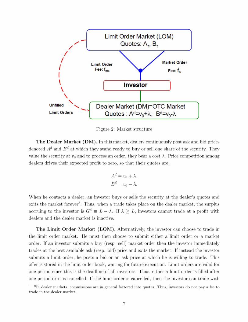
Figure 2: Market structure

The Dealer Market (DM). In this market, dealers continuously post ask and bid prices

denoted Ad and Bd at which they stand ready to buy or sell one share of the security. They

value the security at v0 and to process an order, they bear a cost λ. Price competition among

dealers drives their expected profit to zero, so that their quotes are:

Ad = v0 + λ,

Bd = v0 − λ.

When he contacts a dealer, an investor buys or sells the security at the dealer’s quotes and

exits the market forever8. Thus, when a trade takes place on the dealer market, the surplus

accruing to the investor is Gd ≡ L − λ. If λ ≥ L, investors cannot trade at a profit with

dealers and the dealer market is inactive.

The Limit Order Market (LOM). Alternatively, the investor can choose to trade in

the limit order market. He must then choose to submit either a limit order or a market

order. If an investor submits a buy (resp. sell) market order then the investor immediately

trades at the best available ask (resp. bid) price and exits the market. If instead the investor

submits a limit order, he posts a bid or an ask price at which he is willing to trade. This

offer is stored in the limit order book, waiting for future execution. Limit orders are valid for

one period since this is the deadline of all investors. Thus, either a limit order is filled after

one period or it is cancelled. If the limit order is cancelled, then the investor can trade with

8In dealer markets, commissions are in general factored into quotes. Thus, investors do not pay a fee totrade in the dealer market.

7

a dealer and exits.9 That is, investors with unfilled limit orders use the dealer market in last

resort. Following the terminology used by trading platforms, we call “makers”the investors

posting quotes and “takers” the investors hitting quotes.

The limit order book is the set of offers posted in the limit order market at any point in

time. As limit orders are valid for only one period, at each date τ , the limit order book has

three possible states: (i) it contains a sell limit order, (ii) it contains a buy limit order, or

(iii) it is empty. Let Aτ and Bτ be the ask and bid prices posted in the limit order market at

the beginning of period τ . If there is no sell (buy) limit order in the book, we set Aτ = +∞(Bτ = −∞).

The owner of the limit order market (the “matchmaker”) collects a fee, f , each time a

transaction occurs. For simplicity, we set the cost of processing trades for the matchmaker

to zero. Thus,the exchange fee, f , is the profit earned per trade by the matchmaker. This

exchange fee is split between the two sides (maker/taker) in the transaction as follows: the

taker pays a fraction θ of the exchange fee and the maker pays a fraction (1− θ) of the fee.

Following practice, we refer to fma ≡ (1− θ) · f as the “make fee”and to fta ≡ θ as the “take

fee”. The make/take fee breakdown, θ, can take any value (positive or negative) so that

the make fee or the take fee can be negative. The total fee however is positive (f ≥ 0) as

otherwise the matchmaker would lose money on each trade. Thus, if the make fee is negative

(θ > 1), the take fee is positive and vice versa.

We denote by

Gl def= 2L− f ,

the size of the gains from trade net of the fees charged by the matchmaker. When a trade

takes place on the limit order market, the total surplus is Gl + f > Gd, i.e., conditional on a

trade, the limit order market is a more efficient technology to match buy and sell orders.10

2.2 Equilibrium Types

Upon arriving, an investor can submit a market order, a limit order, or trade in the dealer

market. In making his choice, the investor faces a trade-off between taking the price posted

9If a limit order is unfilled at, say, date τ , there is a small delay (less than one period) between the momentat which the investor with the unfilled limit order exits the market (after trading in the dealer market) andthe moment at which a new investor arrives. Hence, the only exit option for the first investor is to trade witha dealer.

10Studies of bid-ask spreads on Nasdaq and the NYSE when these markets were, respectively, similar to adealer market and a limit order market have shown that the average bid-ask spread on Nasdaq was higherthan on the NYSE, in part because real costs of intermediation were higher on Nasdaq (see Stoll (2000)).The real cost of intermediation in a dealer market includes labor costs but also the cost of capital associatedwith inventory risk. This cost is absent from our model but will add up to the cost of intermediation in thedealer market. Fink et al. (2006) also provides evidence consistent with the view that limit order marketsare less costly trading technologies.

8

by other traders (dealers or limit order traders) or posting a price but bearing a waiting cost

and a risk of non execution. We now analyze the solution to this trade-off. To this end, let

δi ≡ ρ · δi for i ∈ {H,L}. For brevity, we refer to δi as investor i’s discount factor.

Consider a trader with a discount factor δi who arrives at date τ and let Vτ (δi) be the

highest expected payoff that the trader can obtain if he submits a limit order. Intuitively, this

payoff is the same for a buyer or a seller because the two sides of the market are symmetric.

Moreover, Vτ (δH) > Vτ (δL) since a patient investor can always submit the same limit order as

an impatient investor and obtain a strictly larger expected payoff (since her discount factor

is higher).

The trader submits a market order if the payoff of this order is greater than the maximum

payoff with the other choices: a limit order or a trade in the dealer market. For instance, a

seller arriving at date τ submits a market order iff

Bτ − fta − vL ≥Max{Vτ (δi), Gd},

that is:

Bτ ≥ Bτ (δi),

where

Bτ (δi) = vL + fta +Max{Vτ (δi), Gd}. (1)

This cut-off price is the smallest bid price at which a seller arriving at date τ is willing to

submit a sell market order. Using the same reasoning, the highest ask price at which a buyer

arriving at date τ is willing to submit a buy market order is

Aτ (δi) = vH − fta −Max{Vτ (δi), Gd}. (2)

As Vτ (δH) ≥ Vτ (δL), we have Bτ (δH) ≥ Bτ (δL) and Aτ (δH) ≤ Aτ (δL). That is, offers in the

limit order book must be more aggressive to attract market orders from patient investors.

This implies that more aggressively priced limit orders have a higher execution probability.

To see this, suppose that the seller arriving at date τ submits a limit order. Let A be the

price of this order and φ(A) be its execution probability (or “fill rate”). If the next trader

is a seller, the limit order does not execute. If the next trader is a buyer, the limit order

executes with certainty if A ≤ Aτ+1(δH), does not execute if A > Aτ+1(δL), and executes

only if the buyer is impatient otherwise. Hence, conditional on continuation of the trading

9

game at date τ + 1, we have

φ(A) =

φH if A ≤ Aτ+1(δH),

φL if Aτ+1(δH) < A ≤ Aτ+1(δL),

0 if A > Aτ+1(δL),

(3)

with φH = 12

and φL = (1−π)2

. As φ(A) is a decreasing step function, there is a continuum

of offers with the same execution probability. Obviously, for a given execution probability, it

is optimal for the seller to make the highest possible offer. Thus, the seller faces a trade-off

between two offers: an aggressive offer at Aτ+1(δH) and a less aggressive offer at Aτ+1(δL).

The first offer has a higher execution probability (φH > φL) but it yields a smaller surplus

in case of execution. As the seller chooses the offer which yields the highest expected payoff,

we deduce that

Vτ (δi) = Maxk∈{H,L} δi ·(φk(Aτ+1(δk)− fma − vL) + (1− φk)Gd

).

Substituting Aτ+1(δk) by its expression in equation (2), we obtain

Vτ (δi) = δi(Maxk∈{H,L} φk(G

l −Max{Vτ+1(δk), Gd}) + (1− φk)Gd

). (4)

Similarly, a buyer submitting a limit order must optimally choose either an aggressive bid

equal to Bτ+1(δH) with a high fill rate (φH) or a less aggressive bid equal to Bτ+1(δH) with

a low fill rate (φL). By symmetry, the highest expected payoff of the buyer is also given by

equation (4).

We shall focus on stationary equilibria, i.e., equilibria in which traders’ strategies and

therefore their payoffs do not depend on time. Let V ∗(δi) be a trader’s maximal expected

payoff with a limit order in a stationary equilibrium. Equation (4) implies that

V ∗(δi) = δi(Maxk∈{H,L} φk(G

l −Max{V ∗(δk), Gd}) + (1− φk)Gd), for i ∈ {H,L}. (5)

For each value of the parameters, we can then solve for traders’ order placement strategies by

first solving equation (5) for V ∗(·). We then deduce traders’ cut-off prices using equations (1)

and (2) and whether traders choose a limit order with a high or a low execution probabilities

when they submit a limit order.

The equilibrium can have one of five possible types, as shown in Table 1. First, if V ∗(δH) <

Gd, the dealer market “crowds out” the limit order market: investors never submit a limit

order since their expected payoff is too small relative to what they can obtain by trading

upon arrival on the dealer market. As a result no trade happens on the limit order market.

When V ∗(δH) ≥ Gd, patient traders prefer to submit a limit order rather than trading

10

in the dealer market immediately upon arrival.11 Hence, at least when the limit order book

lacks liquidity on their side, patient traders use limit orders in equilibrium. We say that

patient investors are specialized if they only use limit orders. This happens when limit orders

are not aggressively priced so that they attract only impatient investors and have therefore

a low fill rate. Otherwise patient investors are unspecialized : they use both market and limit

orders in equilibrium.

In a symmetric way, we say that impatient investors are specialized if they only use market

orders. This happens when V ∗(δL) < Gd < V ∗(δH). In this case, they hit limit orders placed

by patient investors or, if the limit order book is empty on their side, they trade upon arrival

in the dealer market. If instead, V ∗(δL) > Gd, impatient investors are unspecialized: they

submit limit orders when the limit order book lacks liquidity on their side and they submit

market orders otherwise.

Gd < V ∗(δL). V ∗(δL) < Gd ≤ V ∗(δH) V ∗(δH) < Gd

Fill Rate for Limit Orders High (φH) Low (φL) Low (φL) High (φH) n.a

Patient Investors Unspecialized Specialized Specialized Unspecialized n.a

Impatient Investors Unspecialized Unspecialized Specialized Specialized n.a

Equilibrium Type UPUI (#1) SPUI (#2) SPSI (#3) UPSI (#4) Crowding out (#5)

Table 1:Typology of equilibria

Henceforth, we focus on the case in which parameter values satisfy the following condition:

C.1:2π

1− π(1− δL) < δH − δL <

2π

1− π. (6)

Note that this condition requires π ≤ 13

since δj ∈ (0, 1]. Under Condition C.1, each type of

equilibrium can occur (see next section). In this way, our analysis covers all possible cases

that can emerge in equilibrium. In contrast, for other parameter values, some equilibria do

not exist. The results however still hold when Condition C.1 is not satisfied. Sometimes,

for brevity, we shall refer to an equilibrium by its shorthand, e.g., “#1”for the unspecialized

patient/unspecialized impatient investors equilibrium.

3 Equilibrium for fixed fees

We first describe the conditions under which a given type of equilibrium obtains, holding fixed

the exchange fee and its breakdown between makers and takers. These are endogenized in

11When an investor is indifferent between the two trading venues, we assume that he trades on the limitorder market.

11

subsequent sections. To describe the equilibria, let us define κ0 = 0, κ1 = 2π−(1−π)(δH−δL)2π+δH(1+π)−δL(1−π)

,

κ2 = δL(1−π)2(1−δLπ)

, κ3 = δH(1−π)−2π2(1−2π−δHπ)

, and κ4 = δH2

. Under Condition C.1, κ0 < κ1 ≤ κ2 ≤ κ3 ≤ κ4.

Moreover, let us define

λk ≡ L(1− 2κk), (7)

and

fk(λ) = Max

{0,λ− λkκk

}, for k ∈ {1, 2, 3, 4}, (8)

with f0(λ) = 0. Observe that fk(λ) increases in κk so that f0(λ) ≤ f 1(λ) ≤ f 2(λ) ≤ f 3(λ) ≤f 4(λ).

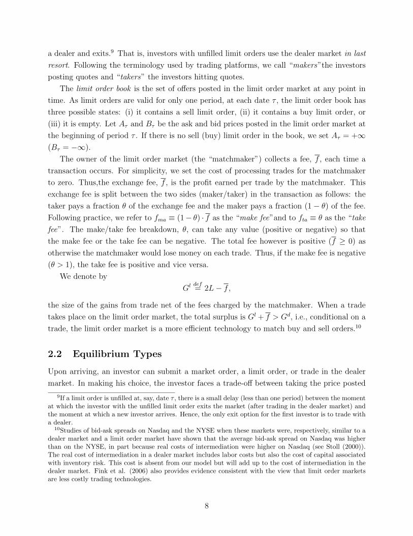
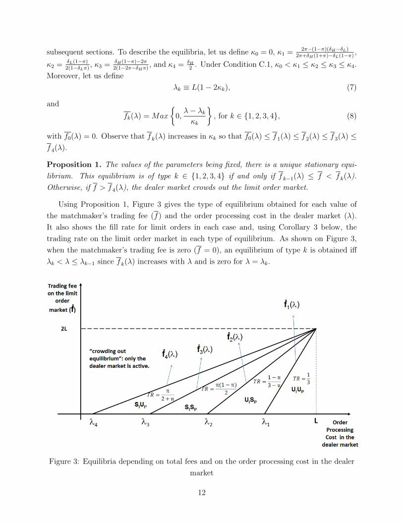
Proposition 1. The values of the parameters being fixed, there is a unique stationary equi-

librium. This equilibrium is of type k ∈ {1, 2, 3, 4} if and only if fk−1(λ) ≤ f < fk(λ).

Otherwise, if f > f 4(λ), the dealer market crowds out the limit order market.

Using Proposition 1, Figure 3 gives the type of equilibrium obtained for each value of

the matchmaker’s trading fee (f) and the order processing cost in the dealer market (λ).

It also shows the fill rate for limit orders in each case and, using Corollary 3 below, the

trading rate on the limit order market in each type of equilibrium. As shown on Figure 3,

when the matchmaker’s trading fee is zero (f = 0), an equilibrium of type k is obtained iff

λk < λ ≤ λk−1 since fk(λ) increases with λ and is zero for λ = λk.

Figure 3: Equilibria depending on total fees and on the order processing cost in the dealer

market

12

Recall that in equilibrium patient and impatient sellers submitting limit orders post the

same ask price while patient and impatient buyers post the same bid price. We denote

the equilibrium ask price by A∗ and the equilibrium bid price by B∗. Due to the model’s

symmetry, these quotes are centered around v0. That is, A∗ = v0 +S∗/2 and B∗ = v0−S∗/2,

where S∗ = A∗−B∗. This spread is the difference between the execution price for buy market

orders and the execution price for sell market orders in equilibrium. Thus, following Stoll

(2000), we refer to S∗ = A∗ −B∗ as the traded bid-ask spread on the limit order market.

Lemma 1. In equilibrium, the traded spread in the limit order market is:

S∗(f, λ, θ) =

2(L− θf − δH

2+δH(3L− f − λ)

)if 0 ≤ f < f 1(λ)

2(L− θf − δL

2+δL(1−π)

((1− π)(2L− f) + (1 + π)(L− λ

))if f 1(λ) ≤ f < f 2(λ)

2(λ− θf

)if f 2(λ) ≤ f < f 3(λ)

2(L− θf − δH

2+δH(3L− f − λ)

)if f 3(λ) ≤ f < f 4(λ)

The traded bid-ask spread does not fully determine the division of gains from trade

between makers and takers because it does not account for take fees. Hence, we also define

the cum fee bid-ask spread, Sc(f, λ, θ), which is the difference between the price cum fee and

the bid price net of fee, that is: Sc(f, λ, θ)def= S∗ + 2fta = S∗ + 2θf . When a trade occurs,

the surplus earned by takers is

vH − (A∗ + fta) = (B∗ − fta)− vL = L− Sc(f, λ, θ)/2 (9)

while makers earn

A∗ − fma − vL = vH − fma −B∗ = L− f + Sc(f, λ, θ)/2 (10)

Thus, a greater cum fee bid-ask spread means that takers capture a smaller share of the gains

from trade available to makers and takers (2L− f). When the limit order market is active,

the cum fee bid-ask spread is always lower than the bid-ask spread on the dealer market

(the two spreads are just equal when f 2(λ) ≤ f < f 3(λ)).12 Otherwise, it would never be

optimal to submit a market order. Moreover the cum fee bid-ask spread is always positive.

In contrast, the total fee being fixed, when the maker fee, fma, is negative and sufficiently

large in absolute value, the traded bid-ask spread can be negative. Yet, buying the security

at the ask price and reselling it at the bid price would not be profitable because, cum fee,

the bid-ask spread is positive.

12The traded spread is S∗ = Sc−2fta. Thus, it is also smaller than the bid-ask spread in the dealer marketwhen fta > 0. In contrast, when fta < 0, the traded bid-ask spread can exceed the bid-ask spread in thedealer market.

13

Corollary 1. 1. The traded bid-ask spread depends on the make/take fee breakdown: it

decreases when takers pay a higher fraction of the total trading fee (∂S∗

∂θ< 0). In

contrast, the cum fee bid-ask spread does not depend on the make/take fee breakdown,

θ (∂Sc

∂θ= 0).

2. The cum fee bid-ask spread increases in the exchange fee, f .

If the platform allocates a higher fraction of the exchange fee to takers then, other things

equal, it becomes more costly to place a market order and more attractive to place a limit

order. Hence, buyers’ cut-off prices decrease whereas sellers’ cut-off prices increase (see

equations (1) and (2)). As a consequence, traders submitting limit orders must post more

attractive quotes and the traded bid-ask spread drops. In equilibrium, this drop is just equal

to the increase in the take fee so that the cum fee bid-ask spread is eventually unchanged

(first part of Corollary 1). The reasoning is symmetric for an increase in the fraction of the

exchange fee allocated to makers.

Hence if the platform changes its make/take fee breakdown, this change is fully neutralized

by the adjustment in equilibrium quotes. Thus, the make/take fee breakdown is neutral: it

does not affect limit order fill rates, the trading rate, and for this reason traders’ ex-ante

expected welfare (see Section 5.1). This result has several empirical implications that we

discuss in Section 5.4.

In contrast, an increase in the exchange fee is not neutral. Obviously, it reduces the net

gains from trade for makers and takers when a trade takes place. Less obviously, as shown

in our two next results, it also affects the likelihood of execution for limit orders and the

trading rate.

Corollary 2. In equilibrium, the fill rate for limit orders is:

FR∗(f, λ) =

φH if 0 ≤ f < f 1(λ)

φL if f 1(λ) ≤ f < f 3(λ)

φH if f 3(λ) ≤ f < f 4(λ)

0 if f > f 4(λ)

Thus, the fill rate for limit orders is a non monotonic function of the exchange fee: it decreases

(from φH to φL) when the trading fee increases from f < f 1(λ) to f ∈ [f 2(λ), f 3(λ)) but it in-

creases again when the trading further increases from f ∈ [f 2(λ), f 3(λ)) to f ∈ [f 3(λ), f 4(λ)].

Thus, the matchmaker’s total fee is one determinant of limit orders’ fill rate. The reason

is that the trading fee affects the relative payoffs of limit orders with high and low execution

probabilities. To see why, let ∆(f) be the difference between the expected payoff of a limit

14

order with a high fill rate and the limit order with a low fill rate, before discounting, i.e.,

∆(f) = φH(Gl − V ∗(δH))− φL(Gl − V ∗(δL))− (φH − φL)Gd. (11)

Now suppose that f 2(λ) ≤ f < f 3(λ). In this case, impatient traders are specialized, so

that V ∗(δL) = Gd and patient investors submit limit orders with a low execution probability,

which means that ∆(f) < 0. Moreover

∂∆

∂f= −(φH − φL)− φH

∂V ∗(δH)

∂f= −π

2− 1

2

∂V ∗(δH)

∂f. (12)

The sign of this derivative is ambiguous because ∂V ∗(δH)

∂f< 0, i.e., an increase in trading

fee reduces the total expected payoff with a limit order in equilibrium. Calculation yields:∂V ∗(δH)

∂f= δH(1−π)

2when f 2(λ) ≤ f < f 3(λ) so that ∂∆

∂f> 0 because δH > 2π

(1−π)(Condition

C.1). Thus, for f 2(λ) ≤ f < f 3(λ), submitting a limit order with a low execution probability

is optimal but the difference between the payoff of this order and the payoff of an order

with a high execution probability shrinks as the trading fee increases. For f = f 3(λ), this

difference is just equal to zero and becomes negative for f > f 3(λ). Thus, when the trading

fee increases from the range f 2(λ) ≤ f < f 3(λ) to the range f 3(λ) ≤ f < f 4(λ), makers

switch from using limit orders with a low execution probability to limit orders with a high

execution probability.

When the limit order market is active, the investor who arrives at a given date can be:

(1) a patient investor who submits a limit order; (2) a patient investor who submits a market

order; (3) an impatient investor who submits a limit order; (4) an impatient investor who

submits a market order; (5) an impatient investor who trades upon arrival in the dealer

market. Let ϕj(λ, f) be the stationary probability of the jth event at date τ in equilibrium

conditional on the asset being still traded at date τ . Hence, the likelihood of a trade on the

limit order market in a given period is

TR(λ, f) = ϕ2(λ, f) + ϕ4(λ, f). (13)

This probability also measures the average number of trades per period on the limit order

market since it gives the fraction of periods in which a trade takes place on the limit order

market. Thus, it measures the trading rate on the limit order market.

15

Corollary 3. In equilibrium, the trading rate in the limit order market is:

TR∗(f, λ) =

13

if 0 ≤ f < f 1(λ)1−π3−π if f 1(λ) ≤ f < f 2(λ)

π(1−π)2

if f 2(λ) ≤ f < f 3(λ)π

2+πif f 3(λ) ≤ f ≤ f 4(λ)

0 if f > f 4(λ)

As π ≤ 13

(Condition C.1), we have π2+π

> π(1−π)2

. Thus, the trading rate increases when

the trading fee switches from the range [f 2(λ), f 3(λ)) to the range [f 3(λ), f 4(λ)]. Indeed, this

switch results in a greater fill rate for limit orders (Corollary 2) and as explained previously,

the increase in the trading fee incentivizes makers to post more aggressive offers. Thus, the

model implies that the trading rate can increase in the exchange fee, for some parameter

values.

4 Inter-market competition and Fees

4.1 Competition between a matchmaker and a dealer market does

not drive the matchmaker’s fee to zero

The per period expected profit of the matchmaker is equal to the trading rate on the limit

order market times the exchange fee per trade on this market. As the trading rate does not

depend on the breakdown of the exchange fee, the matchmaker’s problem is

Maxf

Π(f, λ) ≡ TR(f, λ)× f .

Remember that the trading rate is a step function of the matchmaker’s total fee (see Corollary

3). Thus, there is a continuum of values for f that result in the same trading rate. In this set,

the platform optimally chooses the highest fee. Hence, ultimately, the matchmaker chooses

one among four fees: f 1(λ), f 2(λ), f 3(λ), or f 4(λ), ranked in increasing order (a fee strictly

higher than f 4(λ) results in no trading on the limit order market). Corollary 3 implies that

the trading rate on the limit order market is higher when the matchmaker’s fee is f 4(λ)

than when it is f 3(λ). Hence, the fee f 3(λ) cannot be optimal for the matchmaker since

it generates fewer trades and a lower revenue per trade. In making its choice among the

remaining fees, the platform faces the traditional price-quantity trade-off for a monopolist:

the larger the fee charged by the matchmaker, the smaller the trading rate on the limit

order market. The solution to this trade-off ultimately depends on the order processing

cost in the dealer market, as shown in the next proposition. For this proposition, we use

16

the following notations: λ′1 ≡

((3−π)κ−1

1 −3(1−π)κ−12 −4π

(3−π)κ−11 −3(1−π)κ−1

2

)L, λ

′2 ≡

((2+π)κ−1

1 −3πκ−14 −4(1−π)

(2+π)κ−11 −3πκ−1

4

)L,

λ′3 ≡

((1−π)(2+π)κ−1

2 −π(3−π)κ−14 −4(1−2π)

(1−π)(2+π)κ−12 −π(3−π)κ−1

4

)L. Under C.1, we have either λ

′1 > λ

′2 > λ

′3 > λ4 or

λ′3 > λ

′2 > λ

′1 > λ4.

Proposition 2. 1. If λ < λ4, the limit order market is inactive (there is no positive fee

for which the matchmaker can attract limit orders).

2. If λ ≥ λ4, the matchmaker’s optimal fee is

f∗(λ) =

f 1(λ) if max(λ

′1, λ

′2) ≤ λ ≤ L,

f 2(λ) if λ′3 ≤ λ < λ′1,

f 4(λ) if λ4 ≤ λ < min(λ′2, λ

′3).

Thus, for all values of λ > λ4, the matchmaker’s optimal fee is non competitive (f∗(λ) >

0 for λ > λ4).

Figure 3 shows the optimal fee for the matchmaker as a function of order processing cost

in the dealer market, λ when λ′1 > λ

′2 > λ

′3 > λ

′4. The situation in which λ = L is akin to

the case in which the dealer market does not exist and the matchmaker has therefore full

monopoly power. In this case, the matchmaker leaves no surplus to investors by charging

the largest possible fee: f∗(L) = 2L. When λ < L, the matchmaker must leave a surplus at

least equal to Gd > 0 to investors as otherwise they would trade on the dealer market. For

this reason, the matchmaker’s optimal fee tends to decrease when the order processing cost

in the dealer market declines. Yet, as long as λ is greater than λ4, the fee charged by the

matchmaker is strictly positive. That is, competition from the dealer market is not sufficient

to drive the matchmaker’s profit to zero, unless dealers’ order processing cost is low enough.

The reason is as follows. Liquidity provision is costly both in the dealer market and in

the limit order market. In the dealer market, dealers bear an order processing cost, which is

passed through to investors. In the limit order market there is no order processing cost but

makers bear a waiting cost, which is inversely related to their discount factor. Intuitively

trading in the limit order market is more efficient (i.e., generate higher overall gains from

trade) as long as this waiting cost is not too large compared to the order processing cost,

in particular λ > λ4 = L(1 − δH). The matchmaker can capture part of this efficiency gain

when it is unique in providing the trading technology (a limit order market) enabling traders

to realize this efficiency gain, as assumed so far. Intuitively, the matchmaker’s rent should

vanish if a second matchmaker offers the same trading technology. We now show that this is

the case in the next section.

17

4.2 Competition among matchmakers drives the trading fee to

zero

We now consider the case in which investors can choose to trade on two matchmakers, denoted

1 and 2, rather than just one. The fees and quotes on the platform ran by matchmaker j are

indexed by j ∈ {1, 2}. For instance, f j is the total fee on platform j, θj is the fraction of this

fee paid by takers, and A∗j is the ask price posted by sellers on this platform in equilibrium.

Upon arrival, an investor observes the limit order books of each market and decides whether

to submit a market order, a limit order or to trade on the dealer market. Moreover, if

the investor chooses a market order or a limit order, the investor also decides whether the

order gets routed to matchmaker 1 or to matchmaker 2. When indifferent, we assume that

the investor chooses either market with equal probabilities. The formal definition of the

equilibrium in this case and the proofs of the results in this section are given in the Internet

Appendix, for brevity.

Proposition 3. • If the matchmakers charge different total fees (f 1 6= f 2), the limit

order market with the highest total fee is inactive and the equilibrium is as described in

Section 3 with a single limit order market charging f = Min{f 1, f 2}.

• If the matchmakers charge the same total fees (f 1 = f 2), the equilibrium on each

platform is as described in Section 3 but each platform only attracts half of the trades

because when an investor submits a limit order, he chooses to route his order to platform

1 with probability 12

and to platform 2 with probability 12. Moreover, the platform with

the highest take fee (largest θ) displays a higher bid-ask spread but cum fee bid-ask

spreads are identical on both platforms.

Hence, for a given sequence of investors’ arrivals, the dynamics of order flow in the

consolidated market (i.e., the set of offers/trades in both platforms) does not depend on the

number of competing matchmakers (holding the total fee constant). Thus, the trading rate

in the consolidated market is as given in Corollary 3.13 The second part of the proposition

shows that if both platforms coexist, they must display the same cum fee spread, which

implies that the platform charging the highest take fee must have a smaller traded bid-ask

spread.14 We discuss further this implication of the model in Section 5.4.

13In equilibrium, makers use limit orders with the same execution probabilities on both platforms. Forinstance, if they submit a limit order with high fill rate on platform 1, they also do so when they submitlimit orders on platform 2. Thus limit order fill rates are as given in Corollary 2.

14In addition, the ask price of, say, platform 1 may be equal or smaller than the bid price on platform 2if the make fee on platform 1 is negative. This “locked” or “crossed” markets quotes do not constitute anarbitrage since the true cost of trading cum fees are equal in the two markets. Crossed and locked quotes doarise in reality and several commentators have linked this apparent inefficiency to the practice of subsidizingmakers (see Schmerklen (2003), “Nasdaq’s battle over locked crossed markets,” in Wall Street Technology).

18

Let Πj(f j, f−j;λ) be the expected profit of matchmaker j for a given choice of its fee (f j),

the fee chosen by its competitor (f−j) and the order processing cost in the dealer market.

Using Proposition 3, we deduce that

Πj(f j, f−j;λ) =

TR(f, λ)× f if f j < f−j,

0.5× TR(f, λ)× f if f j = f−j,

0 if f j > f−j.

(14)

The next proposition provides the Nash equilibrium of the game in which the two match-

makers simultaneously choose their trading fees and obtain payoffs given by (14). We focus

on the case λ > λ4 as otherwise the dealer market crowds out the matchmakers.

Proposition 4. : If λ > λ4, both matchmakers optimally choose a zero total fee for any value

of the bid-ask spread in the dealer market. The breakdown of this fee for each matchmaker

is indeterminate (i.e., any menu (fta,j, fma,j) such that fta,j + fma,j = 0 can be sustained in

equilibrium). The type of equilibrium in the consolidated limit order market is as given in

Proposition 1 in the particular case in which f = 0.

Thus, as conjectured, competition among matchmakers drives their trading fees to zero.

In the next section, we show that this is not necessarily good for investors: for some parameter

values, imposing a floor on the trading fee can make them better off.

5 Implications

5.1 Should market forces alone determine exchange fees?

Regulators sometimes intervene in the determination of exchange fees. For instance, in the

U.S., the SEC has capped take fees at $0.0003 per share traded in 2006, as part of RegNMS

and is now considering imposing a similar cap in the options market. For a fixed value of

the trading fee, this amounts to capping θ in our model. This type of intervention is very

controversial. For instance, in reaction to a proposal by the SEC of capping take fees in the

option market, GETCO (a major proprietary trading firm) writes:

“GETCO believes that market forces should determine exchange fees and that the Com-

mission should not allow itself to be drawn into “rate fixing”or “price fixing”. Rather, the

Commission should allow the power of free markets to set exchange pricing.” (see “Comments

Regarding NYSE Arca’s Proposed Rule Change to Amend its Schedule of Fees and Charges

(SR-NYSEArca-2008-075”)

Should one exclusively rely on market forces for the determination of trading fees or is

there room for “rate fixing” by the regulators? To study this question, let W (λ, f) be the

19

expected ex-ante gains from trade for an investor, i.e., before the investor learns his type

(buyer/seller and impatient/patient) and whether he will act as maker or taker (this depends

on the state of the market when he arrives in the market). A maker trades on the limit order

market when he is matched with a taker. Thus, the likelihood that an investor trades on

the limit order is equal to the likelihood of a trade in this market, whether the investor ends

up being the maker or the taker in this transaction. Thus, in absence of “waiting costs” for

makers (i.e., δL = δH = 1), W (λ, f) is the average of (a) the sum of the total gains from trade

when a transaction takes place on the limit order market (i.e., Gl), and (b) the investor’s

surplus when a transaction takes place on the dealer market, Gd, weighted by the probabilities

of each possibility in each period.15 Let, Wbase(λ, f) = TR(f, λ)Gl+(1− 2TR(f, λ))Gd be

this weighted average.16 When δj < 1, an investor’s welfare is smaller than this base level

because makers incur a waiting cost. Computations yield (see the Internet Appendix for the

details):

W (f, λ) = Wbase(λ, f)− (1− δ)(TR(f, λ)× (L−f+Sc/2) + (1− 2TR(f, λ)− ϕ5)×Gd

)︸ ︷︷ ︸

Waiting Costs(15)

where δ is a weighted average of patient and impatient discount factor and ϕ5 is the likelihood

that an investor chooses to trade on the dealer market upon arrival. Investors’ ex-ante welfare

does not depend on the make/take fee breakdown because this breakdown does not affect

the trading rate in the limit order market in equilibrium.

Corollary 4. There exist two thresholds λa ∈ (λ3, λ2] and λb ∈ (λ2, λ3] such that a trading

fee equal to f = f 3(λ) + ε (where ε is very small but positive) maximizes investors’ welfare

when λ ∈ (λ3, λa] or λ ∈ (λ2,λb]. Otherwise, investors’ welfare in equilibrium is maximal

when f = 0.

Thus, there exist values of the parameters for which investors’ ex-ante expected welfare in

equilibrium is maximized when the trading fee is strictly positive. This finding is counterin-

tuitive since, obviously, an increase in the trading fee reduces the gains from trade available

to investors. There is however a less obvious effect: as explained previously, an increase in the

15To understand why, observe that a maker trades on the limit order market when he is matched with ataker. Thus, the likelihood that an investor trades on the limit order is equal to the likelihood of a trade inthis market, whether the investor ends up being the maker or the taker in this transaction. As a result, inabsence of waiting costs, an investor’s welfare is the likelihood that a trade takes place on the limit ordermarket times the total surplus in this case plus the likelihood that a trade takes place on the dealer markettimes the investor’s surplus in this case.

16In each period, a trade happens on the dealer market if (a) the trader arriving in this period immediatelytrade in the dealer market or (b) the limit order placed in the previous period does not execute. Hence, thelikelihood of a trade on the dealer market is ϕ

5(f, λ) +

(ϕ1(f, λ) + ϕ3(f, λ)

)(1−FR(f, λ)) = 1− 2TR(f, λ),

where the last equality is readily obtained using the expression for ϕj given in the proof of Corollary 3.

20

trading fee can induce makers to post offers with a higher fill rate. For instance, suppose that

f = 0 and that λ ∈ (λ3,λ1). In this case, the equilibrium is such that patient investors are

specialized and impatient investors unspecialized. Patient investors choose limit orders with

a low execution probability (φL, see Figure 3) to extract more surplus from takers in case of

execution. Now suppose that the trading fee is increased from f = 0 to a level slightly above

f 3(λ). This increase induces makers to post offers with a higher fill rate (φH , see Figure 3).

This is welfare improving because a high likelihood of execution for limit orders reduces the

number of states in which makers’s waiting cost is paid needlessly. This effect dominates the

reduction in gains from trade due to the higher trading fee when λ3 < λ ≤ λa or λ2 < λ ≤ λb.

Hollifield et al.(2006) show empirically that unfilled limit orders are one important source

of inefficiency in limit order markets. This is also the case in our setting since makers with

unfilled limit orders bear a waiting cost without return on this investment (they end up

trading in the dealer market, something they could have done right upon arrival without

sinking the waiting cost). For some parameter values, an increase in the trading fee can

alleviate this inefficiency because it induces makers to choose limit orders with a higher

execution probability.

Table 2 illustrates this finding with a numerical example. For the values of the parameters

in Table 2, we have λ3 = 0.802, λ2 = 0.95 and λa ≈ 0.84. We therefore show investors’ welfare

when f = 0 (second column) and f = f 3(λ) + ε (third column) for different values of λ in

[0.802, 0.95]. For instance when λ = 0.82, investors’ welfare with a zero fee is equal to about

0.32. It is possible to increase this welfare by 8.5% by setting a fee equal to f = 0.18. This

is a relatively large fee since in our example L = 1, so that the fee accounts for about 9% of

total gains from trade when there is a trade on the limit order market.

Investor’s Welfare

Zero Trading Fee Trading Fee: f 3(λ) + ε Difference (%)

Order Processing Cost: λ

0.81 0.33 0.36 9%

0.82 0.32 0.34 8.5%

0.85 0.30 0.29 -2.2%

0.88 0.27 0.23 -17%

0.90 0.26 0.19 -25%

Table 2: Trading fee and investors’ welfare. For each value of λ shown in the table, we give

investors’ ex-ante expected gains from trade when the trading fee is zero (column 2) and when the trading fee

is slightly above f3(λ)(ε = 10−9). Other parameter values are L = 1,δH = 0.885, δL = 0.067 and π = 0.297 .

21

Corollary 4 raises the intriguing possibility that competition among matchmakers may

be detrimental to investors. Indeed, for values of λ ∈ [λ3, λ1], the equilibrium with two

matchmakers is such that limit orders’ fill rate is low whereas a single matchmaker always

sets its fee such that the fill rate is high. Thus, a priori, a market structure featuring a single

matchmaker coexisting with a dealer market (preventing the matchmaker from extracting

a too large rents from investors) may dominate the market structure with two competing

matchmakers. However, as shown in the next corollary, this never happens because a single

matchmaker’ optimal fee is always too high.

Corollary 5. For all values of the parameters, investors are better off with access to two

competing matchmakers rather than a single matchmaker.

Hence, there is a range of values for λ (λ ∈ (λ3, λa] or λ ∈ (λ2,λb]) where market forces will

not result in the optimal trading fee for investors: with competition among two matchakers,

this fee can be too low (Corollary 4) whereas with competition between a single matchmaker

and a dealer market, this fee is always too high (Corollary 5). For this range of values for

λ, regulatory intervention can make investors better off. The intervention can consist simply

in imposing a floor, equal to ffloor

= f 3(λ) + ε, on the fee charged by the matchmakers, as

shown by the next corollary.

Corollary 6. When λ ∈ (λ3, λa] or λ ∈ (λ2,λa], investors’ welfare is maximal with two

competing matchmakers and a floor on the trading fee equal to f 3(λ) + ε.

5.2 Should limit order markets co-exist with OTC markets?

In the aftermath of the subprime crisis, the G-20 leaders stated that all standardised over-

the-counter (OTC) derivatives contracts should be traded on exchanges or electronic trading

platforms by the end of 2012.17 The effects of such a drastic change in market structure

are much debated, in part because the costs and benefits of limit order markets relative to

OTC markets are not well understood.18 One basic question is whether there are cases in

which imposing concentration of trading in either a limit order market or a dealer market is

optimal.

Our model can be used to study this question. We consider three possible policies: (i)

impose concentration of trading in limit order markets, (ii) impose concentration of trading in

17See Statement No. 13, Leaders’ Statement: The Pittsburgh Summit (September 24 – 25, 2009), availableat http://www.g20.org/ Documents/pittsburgh summit leaders statement 250909.pdf

18There are many aspects of this debate that are beyond the scope of this paper. For instance, tradeson electronic markets are cleared through central clearing counterparties, which reduces counterparty risk.This risk plays no role in our model. For an overview of standard costs and benefits of OTC mar-kets, see, for instance, the report of the International Organization of Securities Commission available athttp://www.iosco.org/library/pubdocs/pdf/IOSCOPD345.pdf

22

the dealer market, or (iii) authorize trading in both market structures (the “hybrid” market

structure). We only consider cases in which investors have access to two matchmakers when

trading in limit order markets is authorized since this market structure always dominates

that with a single matchmaker (Corollary 5). The next proposition gives the policy that

maximizes welfare for each value of λ.

Corollary 7. :

1. When λ ≤ λ4, investors’ welfare is maximal when the regulator imposes concentration

of trading in the dealer market.

2. When λ > λ4, depending on the parameters π, δH , δL: either investors’ welfare is

maximal when the regulator authorizes the hybrid market structure or there exists

λ ∈ (λ4, λ1) such that for λ ∈ [λ, λ1[ investors’ welfare is maximal when the regula-

tor imposes concentration of trading in limit order markets and maximal in the hybrid

market structure otherwise (i.e., for λ ∈ (λ4, λ)⋃

[λ1, L]).

As explained previously, liquidity provision is costly in both trading mechanisms: in the

dealer market, dealers bear an order processing costs whereas makers bear a waiting cost in

the limit order market. Imposing concentration of trading in the dealer market is optimal for

investors when the order processing cost is low enough relative to patient investors’ waiting

cost, λ ≤ λ4 = L(1− δH). Indeed, one benefit of the dealer market is that it enables traders

to save on waiting costs.

Now suppose that λ > λ4 and suppose that the regulator imposes concentration of trading

in limit order markets (the G20 proposal). This situation is as if L = λ. In this case, the

equilibrium is always such that both patient and impatient investors are unspecialized (see

Figure 3). Thus, the fill rate for limit orders and the trading rate are high. Relative to this

market structure, the hybrid market has costs and benefits for investors. One benefit is that

it enables investors with high waiting costs to trade immediately in the dealer market rather

than posting a limit order if the limit order market is not sufficiently liquid when they arrive

in the market. This is what impatient investors do when λ ∈ [λ4, λ2]. Another benefit is that

it mitigates the cost of non execution for makers since they can contact dealers in last resort

to execute their trades. But precisely for this reason, makers optimally post offers with a

low execution probability when λ ∈ [λ3, λ1]. As explained previously, this is detrimental to

welfare. For this reason, there is a range of value for λ (λ ∈ [λ, λ1[) for which investors are

better off when the dealer market is banned.

23

Investor’s Welfare

Regulatory Policy

Hybrid Limit Order Trading Only Dealer Market Only

Order Processing Cost: λ

0.2 0.82∗ 0.35 0.8

0.5 0.60∗ 0.35 0.5

0.7 0.45∗ 0.35 0.3

0.82 0.32% 0.35∗ 0.18

0.99 0.35% 0.35∗ 0.01

Table 3: Market Structure and Investors’ welfare. For various values of λ, we give investors’

ex-ante expected gains from trade in various market structures: two competing matchmakers with a dealer

market, two competing matchmakers, a dealer market only (no matchmakers). A superscript “*”indicates

which structure is optimal for each value of λ. Other parameter values are L = 1, δH = 0.885, δL = 0.067

and π = 0.297.

Table 3 illustrates Corollary 7 for the same parameter values as in Table 2. For these

parameter values, λ4 = 0.11, λ3 = 0.80, λ2 = 0.95, λ1 = 0.98 and λ = λ3. Thus, the optimal

organization for investors features two competing matchmakers operating in parallel with

a dealer market for λ ∈ [λ4, λ3] or λ > λ1, a single dealer market when λ < λ4, and two

competing matchmakers without a dealer market for λ ∈]λ3, λ1[.

5.3 Bid-Ask Spreads and Make/Take Fees

In recent years, much regulatory attention has been devoted to make and take fees and

whether these fees should be regulated or even banned. This regulatory focus may have been

misplaced however if, as implied by our model, the make/take fee breakdown, θ, is neutral,

i.e., if it has no effect on market participants’ welfare. At first glance, this proposition looks

counterintuitive: for instance, rebates for makers should make them better off since they get

a payment in case of execution. Moreover, some market participants argue that these rebates

also benefit takers because they result in smaller bid-ask spreads.19 This effect is present in

our model: an increase in θ leads to a smaller traded bid-ask spread (Corollary 1). However,

the traded bid-ask spread always adjusts to neutralize the effect of a change in θ on the cum

fee bid-ask spread, so that makers and takers’ payoffs in equilibrium do not depend on the

make/take fee breakdown. This yields the following testable implication.

19See again for instance GETCO’s “Comments Regarding NYSE Arca’s Pro-posed Rule Change to Amend its Schedule of Fees and Charges,” available athttp://www.getcollc.com/index.php/getco/commentletters/

24

Implication 1: Holding the total trading fee constant, an increase in the take fee (i.e.,

an increase in θ) reduces the traded bid-ask spread but it has no effect on the cum fee bid-ask

spread.

Testing Implication 1 however is tricky because changes in the make/take fee breakdown

usually coincide with a simultaneous change in the total fee (f). One can therefore wrongly

attribute the observed changes in cum fee bid-ask spreads as being due to the change in

make and take fees whereas in reality these changes are driven by the total fee. To see this

trap, observe that the second part of Corollary 1 has the following implication.

Implication 2: A cut in the total fee reduces the cum fee bid-ask spread whether the

reduction in the total fee is due to a cut in the make fee, a cut in the take fee or a mix of the

two.

We illustrate this point with a numerical example. In Table 4, we compare the traded

bid-ask spread and the cum fee bid-ask spread in equilibrium for two different trading fees,

f = 0.2 and f = 0.1. In the first case, the trading fee is equally split between makers and

takers. In the second case, we consider two distinct scenarios: in the first scenario, the

platform subsidizes makers while in the second scenario it subsidizes takers. Now suppose

that the trading platform reduces its fee from f = 0.2 to f = 0.1. In the first scenario, there

is a drop in the traded bid-ask spread and the cum fee bid-ask spread. As the drop in the

total fee is achieved through the payment of a rebate to makers, it is tempting to attribute

the reduction in the cum fee bid-ask spread to this rebate. This conclusion is misleading

however: the same reduction in the cum fee bid-ask spread can be obtained by paying a

rebate to takers rather than to makers reducing, as seen by considering the second scenario

in Table 4. What matters is the reduction in the total fee, not whether this reduction is

achieved through a smaller make fee or a smaller take fee.

f = 0.2 f = 0.1

Scenario 1 Scenario 2

fma = fta = 0.1 fta = 0.15;fma = −0.1 fta = −0.1; fma = 0.15

Traded Spread 0.54 0.38 0.88

Cum Fee Spread 0.74 0.68 0.68

Table 4: Effect of a cut in the exchange fee on the traded bid-ask spread and the cum fee bid-ask

spread. Parameter values are L = 1, δH = 0.8, δL = 0.5, λ = 0.6, and π = 0.2.

Table 4 also shows that a reduction in the make fee and a reduction in the take fee

have opposite effects on the traded bid-ask spread: the reduction in the make fee reduces

25

the traded bid-ask spread while the reduction in the take fee increases it. This is another

testable implication of the model which follows from the expressions for the traded spread

given in Lemma 1.20

Implication 3. A cut in the take fee increases the traded bid-ask spread while a cut in

the make fee reduces the bid-ask spread. Thus, the effect of a cut in the total fee on the traded

bid-ask spread depends on whether this cut is achieved by decreasing the take fee or the make

fee.

Consider an increase in the take fee, fta. Other things being equal, this increase reduces

one-for-one the concession that investors are willing to pay to trade upon arrival with a

market order. That is, buyers’ cut-off prices decline and sellers’ cut-off prices increase, each

by an amount equal to the take fee (see equations (1) and (2)). As a consequence, investors

submitting limit orders must post more attractive quotes and the traded bid-ask spread

narrows. This reduction in bid-ask spreads implies that the expected payoff with a limit

order drops, which makes investors more willing to pay a concession for immediate execution.

This indirect effect partially, but not fully, countervails the initial change in investors’ cut-off

prices and the bid-ask spread. Thus, the net effect of an increase in the take fee is to reduce

the traded bid-ask spread.

Now consider the effect of an increase in the make fee. Other things equal, an increase

in the make fee reduces the expected payoff of investors submitting limit orders. As a

consequence, all investors are ready to pay larger concessions to get immediate execution.

That is, other things being equal, the buyers’ cut-off price increases and the sellers’ cut-off

price decreases when the make fee increases (see equations (1) and (2)). This effect enables

investors submitting limit orders to charge less competitive quotes, unless their quotes are

constrained by those posted in the dealer market. But this constraint does not bind only

when λ ∈ [λ3, λ2]. Thus, the net effect of an increase in the make fee is to increase the traded

bid-ask spread.

The testable implications derived in this section do not depend on whether we consider a

single matchmaker or two competing matchmakers. Indeed, the second part of Proposition 3

implies that if two matchmakers charge the same total fee, the traded bid-ask spread should

be smaller on the platform with the highest take fee and the cum fee bid-ask spread should

be identical on both platforms. This is just another way to state Implication 3. Moreover, if

one platform reduces its total fee, as in the thought experiments considered in Implications

4 and 5, then it attracts all trades and everything is as if there was a single platform.

It is often argued that a trading platform can increase its market share by tilting its

make/take fee breakdown in favor of makers. The reasoning is that a low make fee attracts

20For this implication, we assume that the platform chooses directly the make fee, fma, and the take fee,fta, rather than θ, as otherwise we cannot vary the make fee independently of the take fee. This is innocuoussince eventually the traded bid-ask spread can be written directly as a function of fma and fta.

26

limit orders who then attract market orders. Proposition 3 (and Implication 1) does not

vindicate this argument: the market share of a matchmaker is independent of its make/take

fee breakdown, θj, and only determined by its total fee relative to its competitor’s fee. To see

why, suppose that initially both platforms have the same make/take breakdown and suppose

that platform 2 decides to shift this breakdown in favor of makers by setting θ2 > θ1. Other

things being equal, the cut in the make fee on platform 2 increases makers’ expected payoff

on this platform. But, for this reason and the fact that the take fee is higher on platform

2, traders now require more attractive quotes to place a market order on platform 2. Thus,

the traded spread on platform 2 must drop relative to the traded spread on platform 1. In

equilibrium, this drop fully neutralizes the change in make/take fees and the cum fee bid-ask

spread is identical on both platforms. At this point, the division of gains from trade between

makers and takers is identical in both markets (as cum fees quotes are identical) and makers

are therefore indifferent between routing their limit orders to platform 1 or platform 2.

In 2005, the Toronto Stock Exchange implemented a new fee structure for a subsets of

stocks listed on this market. Specifically, it started paying a rebate to makers and charged

a fixed take fee of $0.0004 per share. Relative to the previous fee structure, this change was

a clear reduction in trading fee for makers and an increase in the trading fee for takers, for

stocks trading below $22. In contrast, the fee paid by takers was reduced for stocks trading

above $22. These changes in make and take fees also affected the total exchange fee. This

total fee increased for stocks with a price below $6.875 and decreased for stocks with a price

above $6.875. Malinova and Park (2011) provides a detailed empirical analysis of the effects

of these changes on various measures of bid-ask spreads. Interestingly, their findings fit well

with our predictions. In line with our Implication 3, Malinova and Park (2011) find that

effective spreads declined significantly for stocks that experience an decrease in their make

fee and an increase in the take fee (stocks with a price less than $22) but not for stocks

for which the make fee and the take fee declined (see their Table 3). Second Malinova and

Park (2011), Table 5 finds that the cum fee bid-ask spread increased significantly for stocks

that experience an increase in the total exchange fee (i.e., stocks with a price below $6.875).

In contrast, the cum fee bid-ask spread declines (not significantly) for other stocks. These

observations are consistent with our Implication 2.

5.4 Other empirical implications

Another testable implication of our model is that the trading fee charged by the platform

affects the execution probabilities of limit orders. This implication is important as ultimately

this is this effect which explains why counter-intuitively an increase in the trading fee can

raise investors’ welfare. Indeed, as explained in Section 3, the trading fee affects the relative

payoffs of limit orders with high and low execution probabilities. As a result an increase

27

in the trading fee can lead investors to switch from using limit orders with low execution

probabilities to limit orders with high execution probabilities (or vice versa). Consistent

with this implication, Malinova and Park (2011) find that stocks affected by the change in

the trading fee on the Toronto Stock Exchange (see previous section) experienced an increase

in their fill rate.

Relatedly, the model also implies that a decrease in trading fee can trigger a drop in the

likelihood of direct trades among investors as it induces makers to post quotes with a lower

execution probability. For this reason, as shown by the next corollary, entry of a new limit

order market could simultaneously force platforms to cut their fees and increase the fraction

of trades taking place OTC. This is rather counter-intuitive since the cut in trading fees

would appear to make trading on the limit order market more attractive.

Corollary 8. Suppose λ > λ4 and that initially only one matchmaker coexists with the dealer

market.

1. When λ3 ≤ λ < λ2, entry of a new matchmaker reduces the trading rate in the consol-

idated limit order market (i.e., increases the market share of the dealer market).

2. Otherwise, entry of a new matchmaker increases the trading rate in the consolidated

limit order market or has no effect on this rate (i.e., decreases the market share of the

dealer market or has no effect on this share).

Thus, the model predicts that entry of a new limit order market can result in an increase

in the OTC market share (first part of Corollary 8). European equities markets offer an

ideal setting to test this implication. Indeed, until 2007, there was almost no competition for

order flow among stock exchanges in Europe. Very much as in the baseline model, investors

could trade a firm’s stock only in one limit order market (usually the domestic market of

the firm) or on the OTC market. This situation changed in 2007 with the implementation

of new rules (MiFID) facilitating the entry of new trading platforms (Chi-X, BATS etc...).

As a result, trading fees have considerably decreased since 2007. Anedoctal evidence suggest

that this decline coincides with an increase in the market share of OTC equities market for

E.U stocks.21 At first glance, this evolution is puzzling since one would expect the drop in

trading fees to make trading in limit order markets more attractive. Yet, it is a possibility

in our model.

21For instance, in Europe, the market share of OTC trading in equities markets is estimated at 36% (seeFESE (2011)).

28

6 Conclusion

In this paper, we show that trading fees in a limit order market are more than just transfers

from investors to owners of the market. Indeed, they indirectly affect makers’ market power

relative to takers and as a consequence the execution probabilities chosen by investors sub-

mitting limit orders. In particular, an increase in the trading fee on a limit order market has

a non monotonic effect on limit order fill rates. Actually, this increase reduces the surplus

to be split between makers and takers in each transaction. Thus, for a fixed division of this

surplus, it makes the outside option of takers (an immediate trade in a dealer market) more

attractive. As a consequence, makers’ market power is reduced, which, for some parameter

values, induces them to make offers with a higher execution probability. For this reason, a

decrease in trading fees (due for instance to competition among limit order markets) does

not always result in a higher market share for the limit order market or higher expected gains

from trade (as unfilled limit orders result in a welfare loss).

We also use the model to analyze the effect of differentiating trading fees between makers

and takers. This is important since the maker-taker pricing model is very controversial

in the securities industry and the economic rationale for this business model is not well

understood. Moreover, recently, the joint CFTC-SEC task force on the flash crash of May

2010 has advocated differentiating make and take fees according to market conditions: “A

peak load pricing solution to encouraging liquidity could have both access fees and rebates rise

in turbulent markets. If one Exchange has a higher access fee than another, then it will get

fewer aggressive liquidity demanding trades. If an exchange has a higher rebate, it will get a

disproportionate share of liquidity supplying limit orders to fill out its book.” (see Summary

report of the joint CFTC-SEC Advisory Committee on Emerging Regulatory issues, p.9).22

In our model, for a fixed trading fee, a change in the make/take fee breakdown affects

the raw bid-ask spread but it leaves the cum fee bid-ask spread unchanged. For this reason,

it leaves the division of gains from trade between makers and takers unaffected. Thus, the

make/take fee breakdown is neutral: it has no effect on traders’ order placement strategies,

trading volume and welfare with and without competition among matchmakers. Only the

total fee matters.

We see this irrelevance result as a useful benchmark to identify conditions under which

make and take fees would matter. For instance, in our setting, makers face no constraints on

the prices that they can post. In reality, these prices must be posted on a grid with a fixed

minimum price variation (e.g., 1 cent in the U.S). With such a friction, makers cannot fully

neutralize the effect of a change in the make/take fee breakdown and this breakdown should

therefore start playing a role. Foucault, Kadan and Kandel (2009) develop a theory of optimal

22Access fees is another name for take fees and rebates here refer to negative make fees.

29

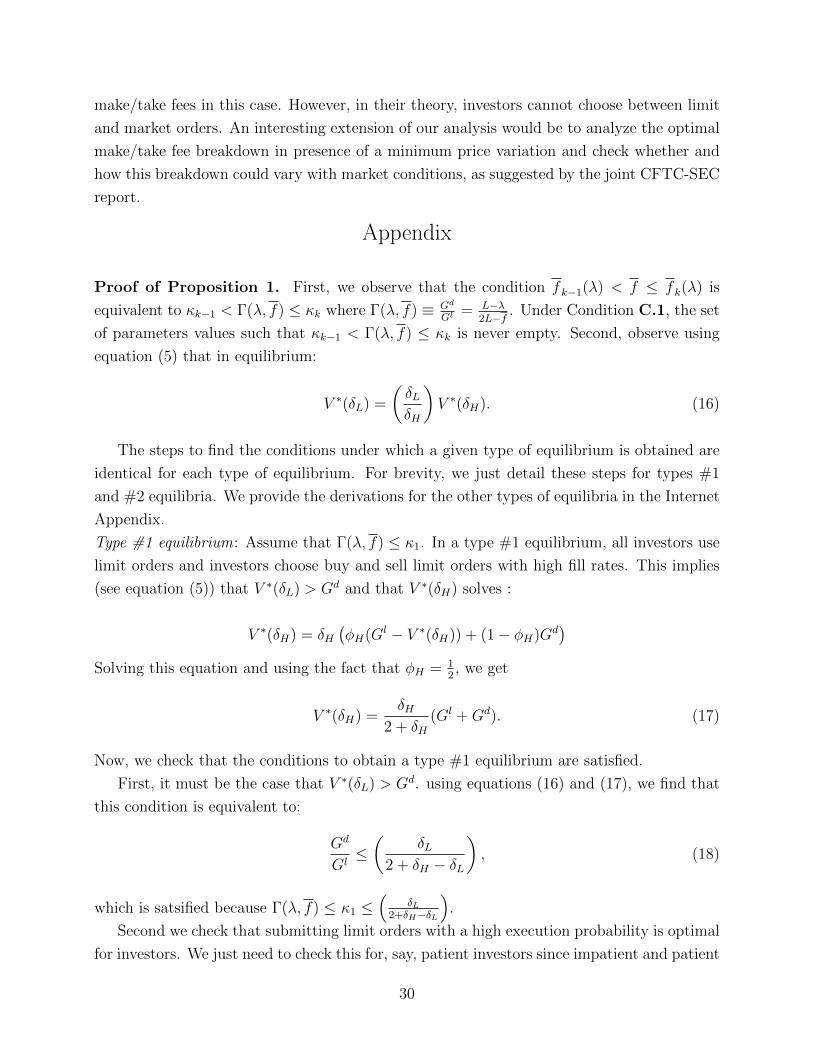
make/take fees in this case. However, in their theory, investors cannot choose between limit

and market orders. An interesting extension of our analysis would be to analyze the optimal

make/take fee breakdown in presence of a minimum price variation and check whether and

how this breakdown could vary with market conditions, as suggested by the joint CFTC-SEC

report.

Appendix

Proof of Proposition 1. First, we observe that the condition fk−1(λ) < f ≤ fk(λ) is

equivalent to κk−1 < Γ(λ, f) ≤ κk where Γ(λ, f) ≡ Gd

Gl = L−λ2L−f . Under Condition C.1, the set

of parameters values such that κk−1 < Γ(λ, f) ≤ κk is never empty. Second, observe using

equation (5) that in equilibrium:

V ∗(δL) =

(δLδH

)V ∗(δH). (16)

The steps to find the conditions under which a given type of equilibrium is obtained are

identical for each type of equilibrium. For brevity, we just detail these steps for types #1

and #2 equilibria. We provide the derivations for the other types of equilibria in the Internet

Appendix.

Type #1 equilibrium: Assume that Γ(λ, f) ≤ κ1. In a type #1 equilibrium, all investors use

limit orders and investors choose buy and sell limit orders with high fill rates. This implies

(see equation (5)) that V ∗(δL) > Gd and that V ∗(δH) solves :

V ∗(δH) = δH(φH(Gl − V ∗(δH)) + (1− φH)Gd

)Solving this equation and using the fact that φH = 1

2, we get

V ∗(δH) =δH

2 + δH(Gl +Gd). (17)

Now, we check that the conditions to obtain a type #1 equilibrium are satisfied.

First, it must be the case that V ∗(δL) > Gd. using equations (16) and (17), we find that

this condition is equivalent to:

Gd

Gl≤(

δL2 + δH − δL

), (18)

which is satsified because Γ(λ, f) ≤ κ1 ≤(

δL2+δH−δL

).

Second we check that submitting limit orders with a high execution probability is optimal

for investors. We just need to check this for, say, patient investors since impatient and patient

30

investors always choose limit orders with the same execution probabilities (if they place one),

as observed in the text. Thus, we must check that

V ∗(δH) > δH(φL(Gl − V ∗(δL)) + (1− φL)Gd

).

That is, using equation (16),

V ∗(δH) > δH(φL(Gl − δLδ−1

H V ∗(δH)) + (1− φL)Gd)

.

After some algrebra, using equation (17) and the fact that φL = 1−π2

, we rewrite this condition

asGd

Gl≤ [2π − (1− π)(δH − δL)]

[2π + (1 + π)δH − (1− π)δL], (19)

that is Γ(λ, f) ≤ κ1.

Type #2 equilibrium: Assume that κ1 < Γ(λ, f) ≤ κ2. In a type #2 equilibrium, all investors

use limit orders and investors choose buy and sell limit orders with low fill rates. This implies

that V ∗(δL) > Gd and that V ∗(δL) solves (see equation (5)):

V ∗(δL) = δL(φL(Gl − V ∗(δL)) + (1− φL)Gd

)Solving this equation and using the fact that φL = 1−π

2, we get

V ∗(δL) =δL

2 + δL(1− π)

((1− π)Gl + (1 + π)Gd

). (20)

Now, we check that the conditions to obtain a type #2 equilibrium are satisfied. First, using

equation (20), it is easily checked that V ∗(δL) ≥ Gd iff Γ(λ, f) ≤ κ2 as assumed in this case.

Second, we check that submitting limit orders with a low execution probability is optimal

for all investors. We just need to check this for, say, impatient investors since impatient and

patient investors always choose limit orders with the same execution probabilities (if they

place one), as already observed. Thus, we must check that

V ∗(δL) > δL(φH(Gl − V ∗(δH)) + (1− φL)Gd

).

After some algrebra, using equation (17) and the fact that φH = 12, we rewrite this condition

as[2π − (1− π)(δH − δL)]

[2π + (1 + π)δH − (1− π)δL]<Gd

Gl, (21)

that is Γ(λ, f) > κ1.�

31

Proof of Lemma 1. Suppose that 0 ≤ f < f 1(λ). In this case, the equilibrium is of type

#1. In both cases, investors choose limit orders with a high execution probability. Thus, in

these cases:

A∗ = A(δH),

B∗ = B(δH).

Using equations (1) and (2) and the fact that V ∗(δH) ≥ Gd (as otherwise patient investors

would not submit limit orders), we deduce that in quilibrium

A∗ −B∗ = vH − vL − 2fta − 2V ∗(δH).

Substituting V ∗(δH) by its expression (see equation (17) in the proof of Proposition 1), we

obtain

A∗ −B∗ = 2

(L− θf − δH

2 + δH(3L− f − λ)

)if 0 ≤ f < f 1(λ).

Other cases are analyzed in the same way. For instance, when f 1(λ) < f < f 2(λ), a type

#2 equilibrium obtains and investors submit limit orders with low execution probabilities.

Thus:

A∗ −B∗ = A(δL)− B(δL) = vH − vL − 2fta − 2V ∗(δL).

We can then obtain the expressions for the bid-ask spread by replacing V ∗(δL) by its expres-

sion in a type #2 equilibrium (equation (20)). For brevity we relegate analyses of the other

cases to the Internet Appendix.�

Proof of Corollary 1. Direct using the expressions for the quotes in Lemma 1.�

Proof of Corollary 2. For each value of the trading fee, we deduce the corresponding

equilibrium type using Proposition 1. Limit order fill rates then follow from Table 1.�

Proof of Corollary 3. Consider the market for the security at date τ . At this date,

this market can be in six possible states: (0) closed because the asset has already paid

its cash-flow; (1) active, a patient investor arrives and submits a limit order; (2) active, a

patient investor arrives and submits a market order; (3) active, an impatient investor arrives

and submits a limit order; (4) active, an impatient investor arrives and submits a market

order; (5) active, an impatient investor arrives and trades upon arrival in the dealer market.

Transitions from one state to another follows a Markov chain with the following transition

matrix, Pk

Pk =

(1 0′

(1− ρ)1 ρMk

).

32

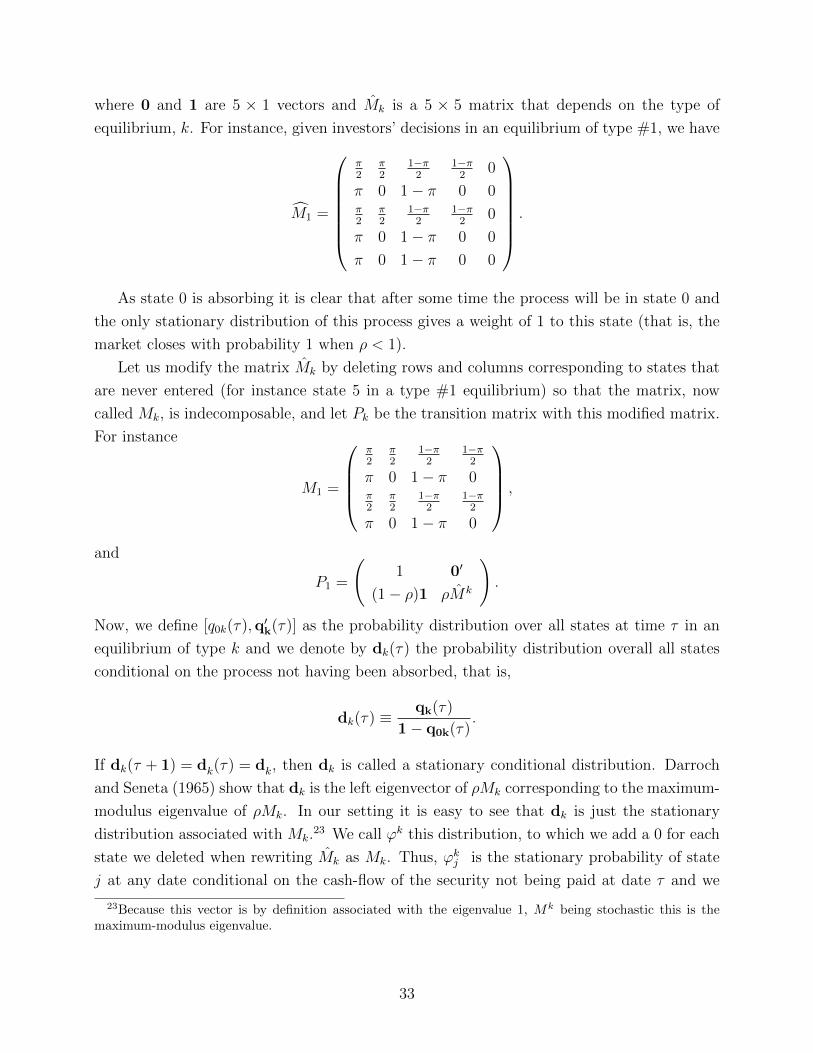
where 0 and 1 are 5 × 1 vectors and Mk is a 5 × 5 matrix that depends on the type of

equilibrium, k. For instance, given investors’ decisions in an equilibrium of type #1, we have

M1 =

π2

π2

1−π2

1−π2

0

π 0 1− π 0 0π2

π2

1−π2

1−π2

0

π 0 1− π 0 0

π 0 1− π 0 0

.

As state 0 is absorbing it is clear that after some time the process will be in state 0 and

the only stationary distribution of this process gives a weight of 1 to this state (that is, the

market closes with probability 1 when ρ < 1).

Let us modify the matrix Mk by deleting rows and columns corresponding to states that

are never entered (for instance state 5 in a type #1 equilibrium) so that the matrix, now

called Mk, is indecomposable, and let Pk be the transition matrix with this modified matrix.

For instance

M1 =

π2

π2

1−π2

1−π2

π 0 1− π 0π2

π2

1−π2

1−π2

π 0 1− π 0

,

and

P1 =

(1 0′

(1− ρ)1 ρMk

).

Now, we define [q0k(τ),q′k(τ)] as the probability distribution over all states at time τ in an

equilibrium of type k and we denote by dk(τ) the probability distribution overall all states

conditional on the process not having been absorbed, that is,

dk(τ) ≡ qk(τ)

1− q0k(τ).

If dk(τ + 1) = dk(τ) = dk, then dk is called a stationary conditional distribution. Darroch

and Seneta (1965) show that dk is the left eigenvector of ρMk corresponding to the maximum-

modulus eigenvalue of ρMk. In our setting it is easy to see that dk is just the stationary

distribution associated with Mk.23 We call ϕk this distribution, to which we add a 0 for each

state we deleted when rewriting Mk as Mk. Thus, ϕkj is the stationary probability of state

j at any date conditional on the cash-flow of the security not being paid at date τ and we

23Because this vector is by definition associated with the eigenvalue 1, Mk being stochastic this is themaximum-modulus eigenvalue.

33

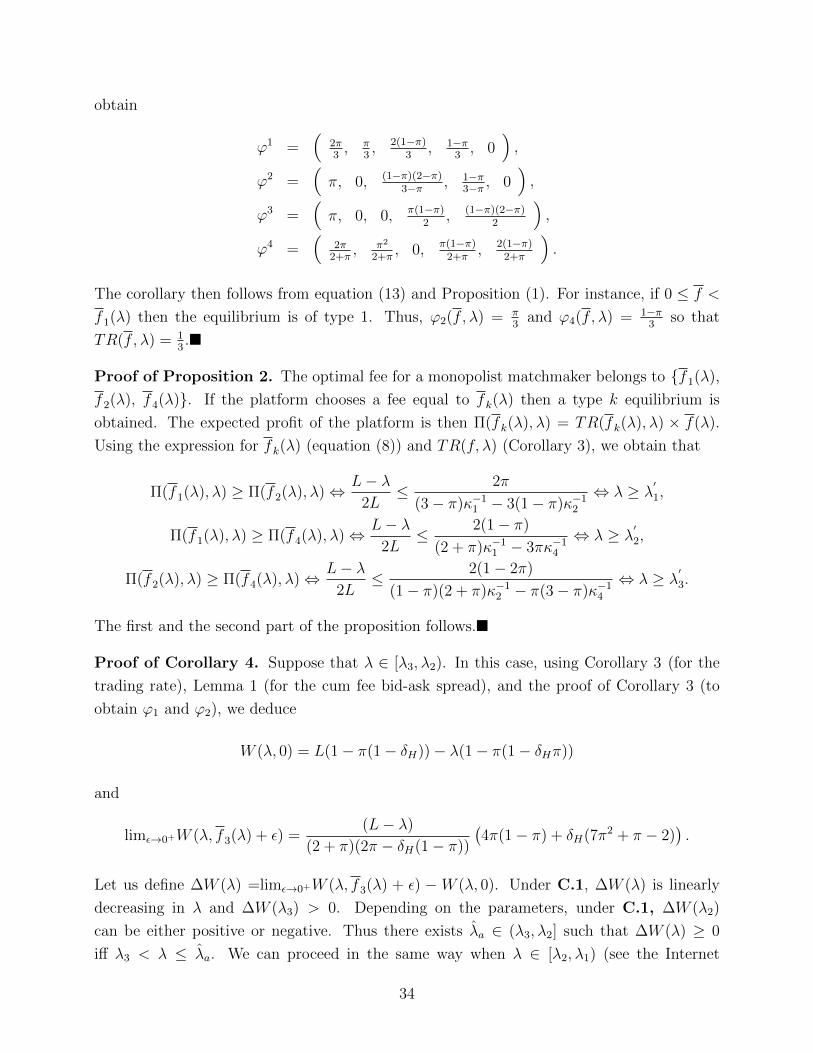
obtain

ϕ1 =(

2π3, π

3, 2(1−π)

3, 1−π

3, 0

),

ϕ2 =(π, 0, (1−π)(2−π)

3−π , 1−π3−π , 0

),

ϕ3 =(π, 0, 0, π(1−π)

2, (1−π)(2−π)

2

),

ϕ4 =(

2π2+π

, π2

2+π, 0, π(1−π)

2+π, 2(1−π)

2+π

).

The corollary then follows from equation (13) and Proposition (1). For instance, if 0 ≤ f <

f 1(λ) then the equilibrium is of type 1. Thus, ϕ2(f, λ) = π3

and ϕ4(f, λ) = 1−π3

so that

TR(f, λ) = 13.�

Proof of Proposition 2. The optimal fee for a monopolist matchmaker belongs to {f 1(λ),

f 2(λ), f 4(λ)}. If the platform chooses a fee equal to fk(λ) then a type k equilibrium is

obtained. The expected profit of the platform is then Π(fk(λ), λ) = TR(fk(λ), λ) × f(λ).

Using the expression for fk(λ) (equation (8)) and TR(f, λ) (Corollary 3), we obtain that

Π(f 1(λ), λ) ≥ Π(f 2(λ), λ)⇔ L− λ2L

≤ 2π

(3− π)κ−11 − 3(1− π)κ−1

2

⇔ λ ≥ λ′

1,

Π(f 1(λ), λ) ≥ Π(f 4(λ), λ)⇔ L− λ2L

≤ 2(1− π)

(2 + π)κ−11 − 3πκ−1

4

⇔ λ ≥ λ′

2,

Π(f 2(λ), λ) ≥ Π(f 4(λ), λ)⇔ L− λ2L

≤ 2(1− 2π)

(1− π)(2 + π)κ−12 − π(3− π)κ−1

4

⇔ λ ≥ λ′

3.

The first and the second part of the proposition follows.�

Proof of Corollary 4. Suppose that λ ∈ [λ3, λ2). In this case, using Corollary 3 (for the

trading rate), Lemma 1 (for the cum fee bid-ask spread), and the proof of Corollary 3 (to

obtain ϕ1 and ϕ2), we deduce

W (λ, 0) = L(1− π(1− δH))− λ(1− π(1− δHπ))

and

limε→0+W (λ, f 3(λ) + ε) =(L− λ)

(2 + π)(2π − δH(1− π))

(4π(1− π) + δH(7π2 + π − 2)

).

Let us define ∆W (λ) =limε→0+W (λ, f 3(λ) + ε) −W (λ, 0). Under C.1, ∆W (λ) is linearly

decreasing in λ and ∆W (λ3) > 0. Depending on the parameters, under C.1, ∆W (λ2)

can be either positive or negative. Thus there exists λa ∈ (λ3, λ2] such that ∆W (λ) ≥ 0

iff λ3 < λ ≤ λa. We can proceed in the same way when λ ∈ [λ2, λ1) (see the Internet

34

Appendix).�

Proof of Corollary 5. The proof consists in showing that W (0, λ) > W (f∗(λ), λ) where

f∗(λ) is given in Proposition 2. This is tedious but straightforward since investors’ welfare

is a linear function of λ. See the Internet appendix for the detailed proof. �

Proof of Corollary 6. Competition among two matchmakers drives their fee to the floor

sets by regulators if this floor is positive. Thus, using Corollary 4, we deduce that setting a

floor equal to f 3(λ) + ε maximizes investors’ welfare when λ ∈ (λ3, λa] or λ ∈ (λ2,λa].�

Proof of Corollary 7. The proof relies on direct comparisons of investors’ welfare under the

different market structures. Although writing investors’ welfare in each market structure is

tedious, comparing the value of investors’ welfare in each market structure is straightforward

since investors’ welfare is a linear function of λ. See the Internet appendix for the detailed

proof. �

References

Barclay, M., T. Hendershott, and T. McCormick, 2003, “Competition among Trading

Venues: Information and Trading on Electronic Communication Networks,” Journal of

Finance, 58, 2637-2665.

Biais, B., C. Bisiere and C. Spatt, 2004, “Imperfect Competition in Financial Mar-

kets”, working paper, Toulouse University.

Boehmer, B. and E. Boehmer, 2004, “Trading your Neighbor’s ETFs’: Competition

and Fragmentation,” Journal of Banking and Finance, 27, 1667-1703.

Cantillon, E. and Yin, P.L., 2010a, “Competition between Exchanges: Lessons from the

Battle of the Bund,” Working paper, MIT and Universite Libre de Bruxelles.

Cantillon, E. and Yin, P.L., 2010b “Competition between Exchanges: A Research

Agenda,” forthcoming International Journal of Industrial Organization.

CFTC-SEC, “Recommendations regarding Regulatory Responses to the Market Event of

May 6, 2010.”

35

Darroch J.N. and E. Seneta, 1965, “On Quasi-Stationary Distributions in Absorb-

ing Discrete-Time Finite Markov Chains,” Journal of Applied Probability, 2 , 88-100.

DeFontnouvelle, P., R. Fishe, and J. Harris, 2003, “The Behavior of Bid-Ask Spreads

and Volume in Options Markets during the Competition for Listings in 1999”, Journal of

Finance, 58, 2437-2463.

Degryse, H., Van Achter, M., and G. Wuyts, 2009, “Dynamic Order Submission

Strategies with Competition between a Dealer Market and a Crossing Network”, Journal

of Financial Economics, 91, 319-338.

Degryse, H., Van Achter, M., and G. Wuyts, 2010, “Internalization, Clearing and

Settlement, and Stock Market Liquidity”, mimeo, Tilburg University.

Duffie, D., Garleanu N., and Perdersen, L. 2009 “Over-the-Counter Markets,” Economet-

rica, 73, 1815-1847.

Federation of European Securities Exchanges, 2011, “Response of the Federation

of European Securities Exchanges to the European Commission Public Consulta-

tion on the Review of the Markets in Financial Instruments Directive” available at

http://www.fese.be/.

Foucault, T., Kadan, O. and Kandel, E., 2010, “Liquidity Cycles, and Make/Take

Fees in Electronic Markets,” Working paper, HEC, Paris.

Foucault Thierry and Albert J. Menkveld, 2008, “Competition for Order Flow and

Smart Order Routing Systems,” Journal of Finance, 63, 119-158.

Gehrig, T., 1993 “Intermediation in Search Markets.” Journal of Economics and

Management Strategy, 2, 97–120.

Glosten, L., 1994, “Is the Electronic Order Book Inevitable”, Journal of Finance,

49, 1127–1161.

Goettler, R. L., C. A. Parlour, and U. Rajan, 2009, “Informed traders and limit

order markets.” Journal of Financial Economics, 93, 67–87.

36

Hendershott, T. and Mendelson, H., 2000, “Crossing Networks and Dealer Markets:

Competition and Performance”, Journal of Finance, 55, 2071-2115.

Hollifield, B., Miller, R. A., and Sandas, P., 2004, “Empirical analysis of limit or-

der markets.” Review of Economic Studies 71, 1027-1063.

Hollifield, B., Miller, R. A., Sandas, P., and slive J., 2006, “Estimating the gains

from trade in limit order markets.” Journal of Finance, 61, 2753-2804.

Malinova, K. and A. Park, 2011, “Subsidizing liquidity: the impact of make and

take fees on market quality,” mimeo, University of Toronto.

Maskin, E. and Tirole, J. (1997) “Markov Perfect Equilibrium: I. Observable Ac-

tions,” Journal of Economic Theory, 191-219.

O’Hara, M. and Ye, M., 2011, “Is market fragmentation harming market quality,”

forthcoming Journal of Financial Economics.

Pagano, M., 1989, “Trading Volume and Asset Liquidity”, Quarterly Journal of

Economics, 104, 255-274.

Parlour, C., and D. Seppi, 2003, “Liquidity-Based Competition for Order Flow”,

Review of Financial Studies, 16, 301-343.

Rust, J. and G. Hall “Middlemen versus Market Makers: A Theory of Competitive

Exchange,” Journal of Political Economy 111, 353-403.

Schmerken I., 2003, “Nasdaq’s battle over locked crossed markets,” Wall Street Technology.

Spulber, D. “Market making by price-setting firms.” Review of Economics Studies

63, 559–80.

Stoll, Hans R., 2000, “Friction”, Journal of Finance, 55, 1479-1514 U.S. Securities

and Exchange Commission, 2000, Release N◦34-42450.

Yavas, A., 1992 “Marketmakers versus matchmakers,” Journal of Financial Inter-

mediation, 2, 33–58.

37