Traders’ Heterogeneity and Bubble-Crash Patterns in

Experimental Asset Markets

Sascha Baghestanian∗, Volodymyr Lugovskyy† and Daniela Puzzello‡

Department of Economics, Indiana University

16th November 2013

Abstract

We provide a heterogeneous agent model for experimental closed-book call-marketswith speculators, fundamental and noise traders. We provide structural estimatesof the parameters of the model using experimental data. The model allows us toidentify the different types of traders empirically. We find that fundamental tradersand speculators have higher cognitive abilities and terminal wealth than noise traders.More importantly, we find that all three types of traders are essential to explain themechanics of bubbles and crashes. In the initial period, fundamental traders buyfrom noise traders. Next, speculators buy from fundamental traders during the boom.Finally, speculators generate the crash by selling to noise traders.

Keywords: Experimental Asset Markets, Bubbles, Trader Heterogen-eityJEL Classifications: C90, C91, D03, G02, G12

∗Department of Economics, Goethe University, House of Finance, Gruneburgplatz 1, Rm

4.12, Frankfurt, Germany; e-mail:baghestanian@econ.uni-frankfurt.de†Department of Economics, Indiana University, Wylie Hall Rm 301, 100 S. Woodlawn,

Bloomington, IN 47405-7104; e-mail: vlugovsk@indiana.edu‡Department of Economics, Indiana University, Wylie Hall Rm 314, 100 S. Woodlawn,

Bloomington, IN 47405-7104; e-mail:dpuzzell@indiana.edu

1

1 Introduction

“There are exceptional people out there who are capable of starting epidemics.

All you have to do is find them.”1

There are several historical examples of bubbles: the Dutch tulip mania (1634-1637), theSouth Sea Company Bubble (1720), the Roaring Twenties stock-market bubble (1922-1929), the Dot-com bubble (1995-2000) and more recently, real-estate bubbles in the USas well as Europe and China. Bubbles generate price distortions that are potentially asso-ciated with allocative inefficiencies and have often led to financial crises. Thus, economistsare naturally drawn towards studying bubbles via theoretical models and empirical meth-ods. Laboratory experiments provide a useful tool to study bubbles empirically sincethey allow economists to control a variety of factors that are difficult to control in fieldenvironments (e.g., trading institutions, the fundamental value process and the dividendprocess).

Bubbles and crashes in experimental asset markets were first documented by Smithet al. [1988] (SSW) and proved to be a very robust result in experimental economics.2

Some authors blame bubbles on speculators (e.g., Smith et al. [1988], Ackert et al. [2006],Moinas and Pouget [2012], Haruvy and Noussair [2006]), while others suggest that subjectconfusion and heterogeneity are responsible for the observed price-swings (e.g., Lei et al.[2001], Kirchler et al. [2012], Caginalp and Ilieva [2005]).3 In general, a clear understandingof the mechanics of bubble formation is still missing. For instance, we do not have manymodels that help us to understand when and why bubbles start and crash (Brunnermeier[2008]).

In order to fill this gap, we propose a heterogeneous agent model which sheds light onthe mechanics of bubble formation in experimental closed-book call markets.4

There are three classes of agents in the model: noise traders, fundamental traders andspeculators. Noise traders are equally likely to be either buyers or sellers in each period,and their bid/ask price is determined by the previous period clearing price plus a noiseterm.5 Fundamental traders buy when the price is below and sell when the price is abovethe fundamental value. Speculators form their price expectations taking into account thepresence of noise traders in the spirit of Level-1 traders. They then buy when the priceis expected to increase and sell otherwise, i.e., their trading behavior is motivated by po-tential capital gains.6 We provide structural estimates of the parameters of the model

1Gladwell [2002].2The bubble-crash pattern persists in treatments with capital gains taxes, no short selling constraints,

transaction fees or the use of a sophisticated subject pool such as corporate managers, professional stocktraders etc. (King et al. [1993], Lei et al. [2001]). Experience of traders in a stationary environment isone of the major factors which dampens or eliminates bubbles under the SSW design (Smith et al. [1988],Porter and Smith [1995], Dufwenberg et al. [2005], Hussam et al. [2008])

3Lei et al. [2001] show that even if capital gains are not possible, the standard bubble-crash patternpersists. Smith et al. [2000] show that if dividends are paid at the end of the trading horizon only (theleast confusing design) the formation of bubbles is least likely. Similarly Kirchler et al. [2012] and Kirchlerand Huber [2011] show that the main source for subject-confusion is the decreasing fundamental valueprocess. Lei and Vesely [2009] show that a pre-trading period before the actual asset market experimentstarts designed to decrease subject confusion about the stochastic dividend process entirely eliminates thebubble-crash pattern.

4For a review of the links between agent-based models and human subject experiments, see Duffy [2006].5In contrast to Duffy’s and Unver’s near-zero-intelligence traders we do not need to assume that noise

traders have weak foresight. This assumption is crucial for Duffy and Unver [2006] to generate the observedcrash-patterns in the lab. In our model it is the interplay of the different trader types which generates thebubble-crash pattern.

6We elaborate below that speculators are similar to Level-1 trader types, characterized by one step

2

using experimental data on five closed-book call market sessions. The estimation is con-ducted by fitting aggregate simulated variables –prices and volume– to the correspondingaggregate experimental variables.

We estimate that 12.5-33% of subjects are speculators, 22-33% of subjects behavelike simulated fundamental traders and the remaining subjects behave like noise traders.We show that simulated fundamental traders accumulate assets early and sell their unitsgradually to speculators and noise traders. Speculators accumulate a substantial numberof assets during the boom and initiate the crash. Simulated fundamental traders andspeculators end up with much lower asset holdings (close to zero) than noise traders.Speculators end up with the the highest simulated terminal wealth levels, followed byfundamental traders. Noise traders end up with significantly lower wealth levels.

The model also allows us to identify traders’ types in the data. Remarkably, we obtaina very clear self-selection of subjects into types, which is consistent with individual charac-teristics of subjects. In particular, fundamental traders are much better in predicting thefirst-period price than other types, and noise traders are much worse in price forecastingduring the crash compared to fundamental traders and speculators. Also, noise tradershave much lower cognitive skills (measured by the Cognitive Reflection Test in Frederick[2005]; CRT) than other types.

Our model and estimation results are instrumental to understanding the mechanicsof experimental bubbles and crashes. In the first period, noise traders under-predict theprice compared to the fundamental value, since they form expectations based on the noiseterm only. As a result, they sell large amounts of the asset to the fundamental traders.After that, speculators buy aggressively (from fundamental and noise traders) since theypredict an upward price trend and expect capital gains. At the peak, which is well abovethe fundamental value, speculators realize the upcoming crash and start selling massivelyto noise traders, who do not foresee the downward price trend. To summarize, noise tradersare first taken advantage of by the fundamental traders and then during the crash by thespeculators. Not surprisingly, they end up with the lowest terminal wealth compared toother classes of traders. Importantly, all three types of traders are essential for explainingthe dynamics of the bubble.

Our work complements the existing literature. The main contribution of our paper,relative to the existing literature, is that we provide a framework that helps understandhow bubbles are generated and crash in experimental asset markets. Specifically, weidentify trading strategies that generate bubble-crash patterns. Relative to Caginalp andIlieva [2005] and Caginalp and Merdan [2007], we emphasize modeling individual beha-vior to capture individual and aggregate features of the data.7 Duffy and Unver [2006]are the first to propose an agent-based model with noise traders to generate bubble-crashpatterns.8 The main departure from Duffy and Unver [2006] is that we introduce hetero-geneous agents and find significant differences in behavior between traders’ types. The mixof heterogeneous agents also allows us to dispense with the assumption of weak foresight

of iterated reasoning in their expectation formation (Stahl and Wilson [1994, 1995], Costa-Gomes andCrawford [2006], Crawford et al. [2013]). In accordance with the Level-k literature we impose that theirrespective anchoring type (commonly referred to as L0-type) are noise traders. In contrast to Haruvy andNoussair [2006] we do not assume that speculators know the specific parameters, which characterize thebehavior of the noise-traders. We assume that they only know the functional form of the equilibrium priceprocess under a trader type distribution degenerate at the noise-trader types.

7Caginalp and Merdan [2007] also provide a heterogeneous agent model for asset markets, which couldin principle be used to generate price dynamics, similar to the ones observed in the lab. However, theirmodel is not suitable to identify whether individual traders indeed belong to certain trader classes ex-post.Hence we would not be able to assess, for instance, the cognitive ability levels of specific individuals,belonging to different groups.

8Duffy and Unver [2006] use the notion “near-zero-intelligence” traders.

3

(the probability of being a buyer decreases with time), which generates the crash in theirenvironment. In our model, the crash is generated endogenously by the interplay of thethree types of traders.9 Haruvy and Noussair [2006] also admit heterogeneous types andadapt the model of DeLong et al. [1990a] into the framework of experimental asset markets.Haruvy and Noussair [2006] focus on fitting price dynamics at the aggregate level, and arenot interested in fitting trading volume paths. Our approach on the other hand allows usnot only to fit trading prices, but also to fit trading volumes at both the individual andaggregate levels.

These differences are essential to improve our understanding of the mechanics ofbubbles and crashes. While a better fit of aggregate variables is a compelling featureof our model, it is not our prime objective. Fitting the trading volume at the individuallevel has substantive implications for the understanding of bubble formation. Indeed, ourwork sheds light on the questions of when and why bubbles start and crash in experimentalasset markets.

Section 2 presents the experimental data. Section 3 presents our model and its mainbuilding blocks. In Section 4 we estimate the parameters of the model based on aggregatevariables. We then proceed and use the estimates to identify different types of tradersin the experimental data. Section 5 shows that bubbles and crashes are generated bythe interplay of speculators, fundamental and noise traders. Section 6 investigates theout-of-sample predictive power of our model. Section 7 concludes the paper.

2 Experimental Design and Data

2.1 Experimental Design and Procedures

The experimental design builds on the seminal study of Smith et al. [1988]. In the laborat-ory market subjects had the opportunity to trade assets with a stochastic dividend process.The market had a finite time horizon of 15 periods. At the end of each period, each unitof the asset in a trader’s inventory paid an uncertain dividend of 0, 8, 28, or 60 francs (theexperimental currency) with equal probability (e.g., Smith et al. [1988], Boening et al.[1993], Caginalp et al. [2000, 2001], Haruvy et al. [2007], Hussam et al. [2008]). Therefore,the expected value of the dividend payment in each period was 24 francs. It was publiclyknown that the dividend was independently drawn each period and the actual dividendpaid in each period was the same for all traders.

Given the dividend process, the fundamental value of the asset could be calculatedat any time within the experiment. More specifically, the fundamental value could becalculated as the expected value of the dividend in each period (24 francs) times thenumber of periods remaining (including the current period). The fundamental value ofthe asset was, therefore, declining from 360 francs in period 1 to 24 francs in period 15,and assets became worthless at the end of period 15. At the beginning of the experiment,each trader was endowed with two units of the asset and a cash balance of 2,000 francs.Traders had the opportunity to buy and sell assets in each period via a closed-book callmarket.10 Subjects could not purchase more units than they could afford nor sell moreunits than they had in their inventories, i.e., negative cash balances and short selling was

9Another difference is that we also focus on a call-market trading institution.10Conditional on asset and cash constraints, subjects submitted buy and/or sell limit orders. Buy orders

were ordered from highest to lowest and sell orders from lowest to highest. The price was determinedby the intersection of these schedules. If they were overlapping, the lowest market clearing price possiblewas then determined to be the trading price in period t, at which transactions were executed. If no suchprice existed, i.e., if the entire demand schedule happened to be below the aggregate supply schedule- thehighest bid-price was reported to the subjects. No transactions were executed at this price.

4

not allowed. Inventories of assets and cash balances were carried over from period toperiod. No interest was paid on cash holdings and there were no transaction costs.

At the beginning of each period traders also made forecasts of the transaction pricefor that period. They were paid for the accuracy of their forecasts.11 All earnings fromforecasting accumulated in a separate account from the traders’ cash on hand, and thusthese payments did not affect the market capital asset ratio.

At the beginning of each session, subjects were provided the instructions of the firsttask of the experiment.12 The instructions for all tasks were projected on an overhead.The first stage in all sessions consisted of a cognitive reflection test (Frederick [2005]) tomeasure the cognitive ability of all subjects. This stage was hand-run with the subjectsproviding their answers to the three questions on a decision sheet. Subjects were given asmuch time as they needed to complete the three questions. Subjects received two dollars foreach correct answer at the end of the session. Once everyone finished, the decisions sheetswere collected and the instructions for the second stage were handed out. The marketinstructions were read aloud in front of the subjects. Afterwards, the subjects were givenfive minutes to complete a short quiz. The experimenter went over the answers on anoverhead and then started the market. The subjects were privately paid their earningsfor all stages of the experiment. Throughout the experiment, subjects were encouraged toask questions at any time. The questions were asked and addressed privately to avoid thepossibility of biasing the entire group.

The experiment consisted of 5 markets conducted at Indiana University. In four outof the five sessions (Sessions 1, 3, 4 and 5) nine subjects participated in the experimentand eight subjects participated in Session 2. Subjects were recruited from undergraduatecourses via the IELab Recruiting System. Many of the subjects had taken part in previousexperiments in economics and other disciplines, but no subjects had participated in mar-kets of comparable designs and each subject participated in only one market of this study.The markets were computerized and programmed with the z-Tree software package.13 Atthe end of a session, each subject’s final holdings of francs were converted to dollars atthe predetermined and publicly known conversion rate of 148 francs to 1 US dollar. Eachsession lasted approximately 80 minutes including instructional period and payment ofsubjects. Subjects earned on average $24.

2.2 Data Description

In this section we focus on the main features of the experimental data. Figure 1 shows theexperimental trading prices for the five sessions and the average price. The lower straightline in the graph depicts the fundamental value of the asset, whereas the higher straightline illustrates the maximum possible value of the asset. We observe that for every sessionthe trading price exceeds this maximum value at least once. The price dynamics show thestandard bubble-crash pattern (e.g., Smith et al. [1988], Boening et al. [1993], Caginalpet al. [2000, 2001], Haruvy et al. [2007], Hussam et al. [2008], and Williams [2008]). Thestandard bubble measures are presented in Table 2. In this paper we provide a modelthat generates price patterns, volume patterns, and bubble measures that are similar tothe observed data.

11They were paid 50 francs for the forecast within 10%, 20 francs for within 25%, and 10 francs forwithin 50% of actual price. We followed Haruvy et al. [2007] for the forecast rewards structure.

12The instructions for all stages of the experiment are available upon request.13See Fischbacher [2007] for a discussion of the z-Tree software package.

5

Figure 1: Time series of transaction prices, all sessions.

3 The Model

We propose a simulation model similar (in spirit) to models suggested by Duffy andUnver [2006] and Haruvy and Noussair [2006].14 We construct the model to resemble thelaboratory economy described in Section 2.

In our market environment N agents interact in T periods and trade a single financialasset. Initially each agent i is endowed with xi0 units of cash and yi0 units of the financialasset. At the end of every period the asset pays random dividends drawn with equalprobability from a commonly known support {d1, d2, d3, d4}, with di ≥ 0 and d1 < d2 <d3 < d4. The expected dividend is denoted as d = 1

4

∑4i=1 di. Since our model is supposed

to fit the laboratory environment, the dividend support is {0, 8, 28, 60}. (In general, thesupport does not necessarily have to be restricted to four values or to an i.i.d. dividendprocess.) The fundamental value of the asset in every period is common knowledge andgiven by

FVt = d(T − t+ 1) for t = 1, ..., T.

Under rational expectations and risk neutrality, prices should equal the fundamental value.

3.1 Simulated Call Market Environment

In this section, we describe the market environment as well as agents’ behavior. In everytrading period t = 1, ..., T traders may either buy or sell units of the financial asset(or remain inactive). During the experiments traders were allowed to submit both bidsand asks simultaneously, potentially for multiple units. To capture this feature in thesimulations, we subdivide each trading period into S submission rounds.

In each of the s = 1, ..., S submission rounds a trader is either a seller or a buyer (thedecision or probability to be buyer or seller is described below). Trader i in submissionround s and trading period t can submit an ask price, ais,t, for one unit of the asset ifshe is a seller and may submit a bid, bis,t, if she is a buyer. These features of the modelallow us to capture the fact that in the experiments traders can submit both bids andasks in a given trading period and to track the volume of the traded asset during the

14See also Gode and Sunder [1993] for goods markets.

6

experiments. Since we do not allow for short-selling or borrowing, in every trading period,traders cannot sell more units than in their holdings, and buyers cannot exceed their cashholdings.

In every submission round in trading period t all the bids and ask prices are aggregatedto obtain the price and quantity traded.15 That is, as in the experiments, the tradinginstitution used to determine market clearing prices is a closed book call market.16

In each round, any buyer who submits a bid above the market-clearing price pst buysone unit of the asset at pst . Thus, the updated cash holdings of a buyer are

xis,t = xis−1,t − pst1(bis,t>pst ),

and similarly the updated unit holdings are

yis,t = yis−1,t + 1(bis,t>pst ),

for each submission round s and trading period t. The symbol 1C is an indicator function,taking the value 1 if condition C is satisfied and 0 otherwise. The assumptions on thebehavior of traders will imply that prices across submission periods ps1t and ps2t withs1 6= s2 will not vary systematically. This particular structure was chosen to account forthe possibility of trading multiple units in a period and to fit the simulated trading volumeto the data.

In each round, any seller who submits an ask below the market-clearing price pst sellsone unit at pst . The updated cash and unit holdings of a seller are

xis,t = xis−1,t + pst1(ais,t<pst )

and

yis,t = yis−1,t − 1(ais,t<pst )

for each submission round s of trading period t.

Next, we explain how market-clearing prices are determined in each submission round.A market-clearing trading price is any price which satisfies

|B| = |{i = 1, ..., N : bis,t > ps,t

}| = |A| = |

{i = 1, ..., N : ais,t < ps,t

}|.17

That is, the market-clearing price is a price at which the number of buyers equals thenumber of sellers. Let bJ be the lowest bid price in B and bJ+1 be the highest bid priceoutside of B. Similarly, let aK be the highest ask in A and aK+1 be the lowest ask outsideof A. Then, for any λ ∈ (0, 1) the following price clears the market:

ps,t = λmin {bJ , aK+1}+ (1− λ) max {bJ+1, aK} . (1)

In the experiments, the market-clearing price was defined as the lowest price at whichthere was an equal number of sellers and buyers. We use λ = 10−2 to determine the

15Bids are ordered from highest to lowest to obtain the inverse demand schedule, while asks are orderedfrom lowest to highest to obtain the inverse supply schedule. The trading price is determined as theintersection of the inverse demand and supply schedules. Note that we can have multiple market clearingprices within a period. The number of rounds fitting the data best is equal to 2, and the average simulateddifference across submission prices within a period is very small, namely, 0.578.

16In closed book call markets traders typically observe only the market clearing price (on their screens)but are not informed about the identities of the traders who sell or buy units of the asset. Typically theyalso do not observe the trading volume in this market environment.

17|U | denotes the cardinality of the set U.

7

corresponding simulation market-clearing price.18 Whenever the entire demand schedulehappened to be below the supply schedule, the highest bid price was taken as a proxy forthe market-clearing price. No trades are executed at this price during the simulations.19

After the Sth (last) submission round in trading period t, the random dividend Dt isrealized and traders update their cash holdings according to:

xi1,t+1 = xiS,t +DtyiS,t.

The period market-clearing price is defined as the average of the sequence of market-clearing prices {pst}

Ss=1:

20

pt =1

S

∑s

pst .

The simulated market-clearing prices will then be compared with the observed market-clearing prices in Section 4.

3.2 Traders

We consider a model with heterogeneous types of traders, namely, noise traders, fun-damental traders and speculators. We need at least three types of traders in order tounderstand the mechanics of bubbles and crashes (see Section 5). We start by describingthe behavior of noise traders. We assume that there are (N−k1−k2) noise traders presentin the market with k1, k2 ∈ {0, 1, ..., N} and k1 + k2 ≤ N . As in Duffy and Unver [2006],we impose some assumptions on the behavior of noise traders and model their biddingbehavior.

At the beginning of every submission round s in every period t, each noise traderis a buyer with probability πt and a seller with probability 1 − πt. We assume thatπt = π = 0.5. We depart from Duffy and Unver [2006] who assume that the probabilityof being a noise-buyer is decreasing over time and initially equal to 0.5. Specifically theyassume that πt = max {0.5− φt, 0} with φ ∈ [0, 0.5T ]. Duffy and Unver [2006] refer to thisas ‘weak foresight’ assumption. This assumption implies that as t increases, the excesssupply increases under weak foresight and generates a downturn of prices. Duffy andUnver [2006] need this assumption to generate the crash pattern, given that their modelconsists of only noise traders. We do not need to impose the ‘weak foresight’ assumptionsince in our model the crash is endogenously generated by the interplay of different typesof traders.

If a noise trader is selected to be a buyer in trading round t and submission period s,she submits a bid subject to cash availability. Her bid is of the form

bn,is,t = min{

(1− α)εt + αpt−1, xis,t

}, (2)

where α ∈ [0, 1], εt ∼ U [0, κFVt], κ ≥ 0 is a parameter, xis,t denotes the current cash

18During the simulations buyers and sellers can submit bids and asks in R+ subject to unit and cashconstraints and not necessarily integer values. The results below are not particularly sensitive to theprecision used in λ. We checked that the results presented below remain fairly unchanged for values ofλ ∈ {0.1, 0.001, 0.0001, 0.000001}.

19In the model, the case in which identical bids or asks are submitted happens with probability zero. Inthis hypothetical case, buyers and/or sellers are determined randomly among agents with identical bids orasks.

20 Note that there are no systematic differences across round market-clearing prices within a period.The average simulated difference across submission prices was 0.578. Recall that we adopt multiple roundsto provide a better fit to the empirically observed trading volumes of the asset.

8

holdings of agent i, and pt−1 is the market-clearing price in period t − 1.21 No bid issubmitted by a noise buyer whenever her cash holdings are zero, i.e., if xis,t = 0.

Similarly, if a noise trader is selected to be a seller in trading round t and submissionperiod s, she submits an ask subject to her unit holdings. Her ask is of the form

an,is,t = (1− α)εt + αpt−1, (3)

where α ∈ (0, 1) and εt ∼ U [0, κFVt]. No ask is submitted by the noise seller wheneverher unit holdings are zero, i.e., if yis,t = 0.

That is, noise traders submit bids and asks based on the previous period price and anoise term, The parameter α ∈ (0, 1) captures the behavioral notion that anchoring effectsmay be important - in our context the relevant anchor is the market clearing unit price inthe previous period.

If we ignore the possibility that unit or cash constraints can be binding, then it isstraightforward to show that, if there are only noise traders, the market-clearing priceconverges to κFVt

2 . If κ = 2, then market-clearing prices converge to the fundamentalvalue. A value of κ > 2 indicates that traders are willing to pay on average more than thefundamental value of the asset to obtain some units of it.

The fact that unit and cash constraints can be binding adds an additional layer tothe problem, which may create substantial deviations from the fundamental value of theasset even if κ = 2. To see this, notice that in a cash-rich environment (cash constraintsnever bind) with a relatively low number of units, prices tend to be higher than thefundamental value of the asset, creating a bubble through the endowment channel. Theintuition is straightforward - suppose for simplicity that S = 1: with low unit holdingsthe probability that some agent with zero asset holdings is selected as a seller in sometrading round is positive. This could create aggregate excess demand, which can only beoffset by a corresponding increase in prices. In other words, even an environment withonly noise traders is sufficiently interesting to address some questions related to aggregateprice variables, as also shown in Duffy and Unver [2006] in the context of a double-auctiontrading institution.

However, adding k2 speculators and k1 fundamental traders provides new insightson price and volume dynamics and thus on bubble formation. Fundamental traders area combination of classes of agents suggested by Cason [1992] and Haruvy and Noussair[2006].

Cason [1992] provides a simulation model for goods markets where market-clearingprices are determined via a closed-book call market institution. In his model, buyerswith random valuation v for the good submit bids which are randomly drawn from aninterval [lt, v]. Buyers adaptively update the lower bound of the interval according tolt = (1− αc)lt−1 + αcpt−1, where pt−1 is the market-clearing price in period t− 1 and theinitial value l0 is the lowest feasible contract price.

Sellers with a random cost parameter c submit asks drawn from an interval [c, at] withat = (1−β)at−1 +βpt−1, where a0 is the highest feasible contract price. For β, αc ∈ (0, 1),Cason shows that the lower/upper bounds of the intervals converge to the competitiveequilibrium price pt if t→∞. The rate of convergence and therefore the speed of learningis determined by αc and β. The lower those two parameters the faster the convergence.Cason further shows that agents behaving according to this rule produce trading pricessimilar to the ones observed in experimental goods markets under a closed book call marketstructure resulting in high efficiency levels.

21We assume that p0 = 0. We will show below that this assumption does not affect our results signific-antly.

9

Haruvy and Noussair [2006] present a simulation model for double auctions assetmarkets. The authors define passive investors as traders who buy assets at the currentstanding ask price if that price is below the fundamental value. Similarly, they sell assetswhenever the current standing bid price is above the fundamental value of the stock. Thetask for fundamental traders under a closed book call market structure is significantlymore complex than under a double auction institution since at the point of the bid/asksubmission, no bids and asks are observed.22

We therefore had to develop a method to characterize the beliefs of fundamentaltraders about the period t market-clearing price given their limited information.

We modify the adaptive agents considered by Cason [1992] and the passive investorsconsidered by Haruvy and Noussair [2006] to model adaptive fundamental or simply fun-damental traders. A fundamental trader computes in every period the bound

lt = αf (lt−1 − d) + (1− αf )pt−1,

with l0 = FV1 + d. The intuition is straightforward: lt serves as a proxy for the expectedmarket-clearing price in period t, which is unknown by the agent at the time of the bid/ask submission. We subtract d to control for the decreasing fundamental value and thusour updating rule for lt differs from the one suggested by Cason [1992]. Notice that ltdoes not depend on s, i.e., we do not allow fundamental traders to learn within the period,which is in line with the experimental design. The functional form of lt suggests thatprice expectations are formed adaptively. Empirical evidence for adaptive expectationformation, used by subjects during asset market experiments, is provided by Haruvy et al.[2007], Smith et al. [1988] and Williams [1987].

While noise traders are randomly determined to be buyers or sellers, a fundamentaltrader decides whether to be a buyer or a seller. If the bound is below the fundamentalvalue, lt ≤ FVt, and her cash holdings are positive, xs,t > 0, then she chooses to be abuyer and submits a bid as follows:

bf,is,t = min{Bis,t, xs,t

}Bis,t ∼ U [lt, FVt]. (4)

That is, if the trader believes that the market-clearing price is below the fundamentalvalue, she submits a bid bf,is,t ∈ [lt, FVt] if she has enough cash. If, on the other hand,the bound is above the fundamental value, lt > FVt, and her asset holdings are positive,ys,t > 0, then she chooses to be a seller and submits an ask from the interval between thefundamental value and the bound:

af,is,t ∼ U [FVt, lt]. (5)

Bids and asks are random to allow for some decision errors.Naturally, if agents cash hold-ings are zero, xs,t = 0, given lt ≤ FVt she does not submit a bid, and if her asset holdingsare zero, ys,t = 0, given lt > FVt, she does not submit an ask.

We also introduce k2 speculators into the model. Speculator j decides whether to buyor sell assets based on her expectations about market clearing prices in period t and periodt+1. Notice that a speculator has to form the relevant expectations before submitting anask or bid order. If

Ejt−1(pt+1) > Ejt−1(pt)

speculator j decides to submit a bid order expecting to make capital gains by selling inthe following period. At this point we do not further specify the expectations operator

22Further, we show in section 11.1 that we cannot reject that there are no participants in our subjectpool, behaving as if they were passive traders with rational expectations.

10

Ej but emphasize that the expectations do not depend on the submission round s. Amore detailed discussion follows below. Intentionally successful and profitable bids –fromthe perspective of the speculator– are in the interval [Ejt−1(pt), E

jt−1(pt+1)]. Allowing for

decision errors we specify that speculators submit bids of the following form:

bsp,is,t = min{Bjs,t, xs,t

}Bjs,t ∼ U [Ejt−1(pt), E

jt−1(pt+1)]. (6)

If on the other handEjt−1(pt+1) ≤ Ejt−1(pt)

speculator j decides to sell and submits an ask order of the form:

asp,is,t ∼ U [Ejt−1(pt+1), Ejt−1(pt)]. (7)

If a speculator’s cash holdings are zero, xs,t = 0, even if Ejt−1(pt+1) > Ejt−1(pt), she

does not submit a bid, and if her asset holdings are zero, ys,t = 0, even if Ejt−1(pt+1) ≤Ejt−1(pt), she does not submit an ask.23

We use a level-k modeling approach to compute speculators’ expectations.24 Specificallywe assume that speculators are level-1 traders, best responding against a benchmark pop-ulation of level-0 noise traders. The average equilibrium price process in a populationconsisting solely of noise traders takes the form:

Et−1(pt) = αpt−1 + (1− α)κ

2FVt

The assumption that speculators know the actual values of α and κ is too strong, especiallyin a closed book call market. We therefore assume that speculator j forms expectationsin the following way:

Ejt−1(pt) = γ1pt−1 + γ2FVt (8)

with γ1 ∈ [0, 1] and γ2 ≥ 0. Iterating (8) one period forward yields Ejt−1(pt+1) as a functionof publicly observed variables, namely, FVt, FVt+1 and pt−1. Note that speculators keepbuying the asset as long as:25

γ1(1− γ1)pt−1 < γ2(γ1(T − t+ 1)d− d). (9)

Since the right hand side of (9) decreases monotonically over time, it is generally possibleto find parameter-values under which speculators initially buy the asset and sell it towardsthe end of the trading horizon. Since fundamental traders sell their assets while pricesincrease well beyond the FV and noise traders follow the price trend, it is the change inthe behavior of speculators, which induces the crash in our model.

We next summarize the simulations steps within a period t :

1. At the beginning of submission round s ∈ {1, ..., S} each of the (N − k1 − k2) noisetraders is determined to be a buyer or a seller according to the probability π = 0.5.Noise buyers submit bids and noise sellers submit asks according to the rules specifiedin (2) and (3).

23We further impose that asp,is,t = FVt in the last two periods of the simulation, whenever a speculatoris a seller.

24See for instance Stahl and Wilson [1994, 1995], Crawford and Iriberri [2007], Crawford et al. [2013].25Note that iterating the expected prices forward yields: γ1(γ1pt−1 + γ2FVt) + γ2FVt+1 which is greater

than Et−1(pt) (in which case speculators buy) iff

γ1(1− γ1)pt−1 < γ2(γ1(T − t+ 1)d− d).

(Using that FVt+1 = FVt − d and FVt = (T − t+ 1)d.)

11

2. Simultaneously, each of the k1 fundamental traders computes lt and decides to beeither a buyer (if lt ≤ FVt) or a seller (if lt > FVt). Depending on this decision, afundamental trader submits either a bid or an ask according to the rules stated in(4) and (5).

3. Simultaneously, each of the k2 speculators computes Ejt−1(pt) and Ejt−1(pt+1) based

on (8) and decides to be either a buyer (if Ejt−1(pt+1) > Ejt−1(pt)) or a seller (if

Ejt−1(pt+1) ≤ Ejt−1(pt)). Depending on this decision, a speculator submits either abid or an ask according to the rules stated in (6) and (7).

4. After all the bids and asks are submitted, the market-clearing price is computed.The market-clearing price is then reported (no additional information is revealed tothe traders) and trades are executed. Traders’ cash and unit holdings are updatedaccordingly.

5. The process above is repeated for the S submission rounds. After trades in theSth submission round are executed, the asset pays its random dividends and cashholdings are updated accordingly.

For a given set of parameters (S, α, κ, αf , k1, k2, γ1, γ2) and experimental characteristics,

N,T and endowments ({xi0}Ni=1

,{yi0}Ni=1

), each simulation run M of the model will gen-

erate a price sequence (pM1 , pM2 , ..., p

MT ), an N × T matrix of cash holdings and an N × T

matrix of asset holdings. The results can be interpreted as the simulation-equivalent ofone experimental session. We next show how to estimate the parameters of the modelusing our experimental data.

4 Model and Data: Estimation

In this section, we estimate the parameters of the structural model using only aggregateprices and quantities. Based on this optimal fit with respect to aggregate variables, wecharacterize the strategies used by speculators, fundamental and noise traders. The resultsare then used to identify the different types of traders in the data. We will show thatthere is a tight relationship between the terminal wealth levels of agents and their tradingstrategies in the simulations, which is also confirmed by the experimental data.

We start by obtaining estimates for the model parameters. Given the initial cash andasset-holdings endowment from the experimental design (2000 francs and 2 units), thenumber of traders N and the number of trading periods T , the model presented in Section2 consists of eight free parameters: the number of submission rounds S, the anchoringparameter of the noise traders α, the noise-support parameter κ of the noise traders, thelearning speed parameter of the fundamental traders αf , the expectations parameters forspeculators γ1 and γ2, the number of fundamental traders k1 and the number of speculatorsk2. We imposed the restriction that

αf = α

to reduce the dimensionality of the parameters.26 In order to obtain parameter estimates,we specified a grid for the parameters S, k1 and k2 and used an interior-point algorithm(Byrd et al. [1999, 2000], Waltz et al. [2006]) to estimate the remaining parameters27 by

26Earlier estimation results indicated that for unrestricted estimations α and αf tend to be very similarin magnitude.

27S ∈ {1, 2, 3, 4, 5} , k1 , k2 ∈ {1, 2, 3, ..., 9}. We used several hundreds of initial starting values to ensurethat we achieved a global minimum.

12

minimizing the following objective function:

SSE(S, α, γ1, γ2, κ, k1, k2) = (10)

15∑t=1

5∑i=1

(p(S, α, γ1, γ2, κ, k1, k2)− pEi,t

FV1)2 +

15∑t=1

5∑i=1

(Q(S, α, γ1, γ2, κ, k1, k2)

Mt −QEi,t

TSU)2,

where p(S, α, γ1, γ2, κ, k1, k2)Mt is the average simulated asset price in period t using M =

100 and some values for the parameters (S, α, γ1, γ2, κ, k1, k2), pEi,t is the price of the asset in

period t and session i. Similarly, Q(S, α, γ1, γ2, κ, k1, k2)Mt denotes the average simulated

trading volume in period t, and QEi,t is the observed trading volume in period t and session

i.28 Equation (10) computes the sum of the squared differences of the simulated averagevariables to the corresponding observed variables. Notice that all our parameters areidentifiable since we have ten observables (the price and quantity data from five sessions)to estimate seven parameters.

Table 1: Estimation Results

α κ S γ1 γ2 k1 k2

0.820 4.915 2 0.256 0.036 22% 22%

Table 1 provides the “best fit” parameter combination. According to Table 1, 22% ofthe traders in our model behave like fundamental traders who learn the market-clearingprice process relatively slowly (α = 0.820). Note that the estimated parameter-value isvery close to the corresponding value for α provided by Duffy and Unver [2006] (0.848),who consider a model with noise traders only.29 The noise amplitude parameter κ, whichmeasures the degree of confusion among noise-traders, takes a value of 4.915 and is againvery close to the corresponding parameter estimate provided by Duffy and Unver [2006](4.085).30 However, we also observe that there are not only noise-traders in our data.44% of our traders are either speculators or fundamental traders. Based on the parameterestimates for γ1 and γ2, we assert that speculators anchor their expectations towards theprevious prices but less than noise traders and do not put a large weight on the fundamentalvalue of the asset. Importantly, we fit the aggregate variables of the model to the data anddo not restrict any behavior of the agents nor do we directly fit the individual behavior ofsimulated agents to the observed behavior of experimental subjects.31

28We normalized the former squared difference by the fundamental value of period 1 and the latterdifference by the total stock of units (TSU). Sessions 1,3,4 and 5 had a TSU of 18 and session 2 had aTSU of 16 since the number of agents in session 2 is eight instead of nine. We used TSU = 18 to obtainparameter estimates, which produce prices and quantities during the simulations, which fit the data. Thatis, we treat session 2 as if it was generated by nine traders. A different approach would be to normalizeby the average TSU across sessions – the difference in the results is negligible.

29See page 13 in Duffy and Unver [2006].30Again, see page 13 in Duffy and Unver [2006].31Our results are robust to relaxing the assumption of p0 = 0. If we ignore the first period price and

volume data our adjusted objective function becomes

SSE(S, α, γ1, γ2, κ, k1, k2) =

15∑t=2

5∑i=1

(p(S, α, γ1, γ2, κ, k1, k2)Mt − pEi,t

FV2)2+

15∑t=2

5∑i=1

(Q(S, α, γ1, γ2, κ, k1, k2)Mt −QEi,t

TSU)2

with FV2 = 336. We re-estimated the resulting objective function and do not find substantial differencesin the resulting parameter estimates.

13

(a) (b)

Figure 2: Data and simulated aggregate variables. Dashed lines: Simulations. Solid lines:Data. Solid straight line: FV. Figure (a): Prices. Figure (b): Volume.

Table 2 provides several bubble measures computed using the data and the model.A quick look at the simulated bubble measures reveals that they are indeed close to theactual data measures. Figure 2 also depicts the simulated and actual prices and quantities.

Surprisingly, there are only two models that provide a theoretical framework forbubbles in experimental asset markets. In what follows we discuss how we contributeto this literature. Duffy and Unver [2006] and Haruvy and Noussair [2006] propose agent-based models which provide a good fit to the aggregate price data. In addition to fittingcrucial elements of the data,32 we would like to emphasize that our model is built tounderstand which trading strategies generate bubble-crash patterns in experimental assetmarkets.

Overall, our model explains various features of the data better than a model withonly near-zero intelligence (NZI) traders modeled as in Duffy and Unver [2006]. Duffy andUnver [2006] allowed for weak foresight assuming that πt = max {0.5− φt, 0}. The relevantparameters of a model with only noise traders in a closed book call market environment are(S, φ, κ, α). We performed the same estimation procedure as above to obtain estimatesfor the relevant parameters and to obtain a closed book call market analogue of themodel consider by Duffy and Unver [2006]. In order to test which model provides abetter fit, we conducted two different tests which focus on average prices. First, wetested for cointegration of the simulated average prices and the observed average pricesusing a Johansen [1991] approach.33 We cannot reject the null hypothesis that the averagesimulated prices from our model are cointegrated with the observed average prices (p-value< 0.05). On the other hand, the prices stemming from the model-specification with onlyNZI traders are not cointegrated with the actual price data at a 10% level. This revealsthat prices in the model with only NZI traders and observed prices follow independentrandom walks. We acknowledge that this result might be driven by the small sample size.Hence we assumed a common stochastic trend between the two time series and performeda standard J-test (Davidson and MacKinnon [1981]) to compare our model with a model,which considers only NZI traders as in Duffy and Unver [2006]. This approach suggests

32Prices, trading volume and final wealth distributions.33We cannot reject the null hypothesis that either of the simulated average prices nor the observed

average prices follow a unit root process using a standard augmented Dickey Fuller test.

14

Table 2: Bubble Measures: Call Markets, 5 Sessions

Bubble Measure Formula Data Simulation

Mean (Std. Err) with Fund. & Speculators

Turnover∑15

t=1 qt/TSU 2.00 2.38(0.41)

Amplitude maxt

{(Pt−FVt)

FV1

}−mint

{(Pt−FVt)

FV1

}5.11 6.49

(3.9)

Total Dispersion∑15

t=1 |median(Pt)− FVt| 2782 2642(993.66)

Average Bias 115

∑15t=1(median(Pt)− FVt) 180.55 215.58

(65.96)

APD 1TSU

∑15t=1 |Pt − FVt| 158.88 163.33

(57.76)

PD 1TSU

∑15t=1(Pt − FVt) 154.64 146.77

(57.31)

RAD 115

∑15t=1

|Pt−FVt|mean(FV )

0.97 1.02

(0.35)

RD 115

∑15t=1

(Pt−FVt)mean(FV )

0.94 0.92

(0.34)

RPAD 115

∑15t=1

|Pt−FVt|FVt

: 1.45 1.71

(0.72)

Haessel R2 of OLS regression: 0.29 0.17Pt = α + βFVt + εt (0.25 )

Boom max{N :

{Pj+k

}Nk=0

>>{FVj+k

}Nk=0

}13.2 14

(1.3)Trend Dur. max

{N : Pt − Ft < Pt+1 − FVt+1 < ... 5.8 7

< Pt−(N−1) − FVt+N−1

}(2.86)

that we can reject a model with NZI traders only in favor of our model at a 1% (p-value= 0.004).34 Out of sample predictions of our model and their fits–using the estimates fromTable 1– are presented in Section 6.

Our model also improves upon the heterogeneous trader-types model used by Haruvyand Noussair [2006], which is based on the standard setup introduced by DeLong et al.[1990a]. First, Haruvy and Noussair [2006] significantly underestimate the observed trad-ing volume in 20 out of their 22 sessions (compare the Turnover between Tables II andIII against Table VIII in their paper). We show below that an accurate estimation of theturnover and dynamic patterns of the trading volume is essential for our understandingof bubbles and crashes. Second, their model does not generate final wealth distributionsacross trader types which mimic the actual wealth distributions, indicating that somebehavioral aspects are missing in their model.

Lastly, the model considered by Haruvy and Noussair [2006] cannot be used to analyzethe impact of different trading institutions on trading strategies. Within every simulation-period Haruvy and Noussair [2006] use a Tatonnement algorithm to find the unique marketclearing price through quantity alterations and fit this price to the average observed tradingprice stemming from double auction experiments. Lugovskyy et al. [2011] show that achange of trading institutions from double-auctions to Tatonnement affects behavior andmay reduce bubbles. In other words, bubbles and crashes are not institution-invariantand it is desirable to construct a model, which may address this issue. While the modelsuggested by Haruvy and Noussair [2006] does not account for those differences, our modelcan be extended easily to analyze the impact of trading institutions in future work.

4.1 Simulated and Experimental Strategy Comparison

In this section, we use our estimates (see Table 1) to compare the simulated individualbehavior to the actual behavior of traders. The main message of this section is that themodel does a good job at describing individual data, even though the parameters are

34See Appendix C for details.

15

(a) (b)

Figure 3: Simulated asset-holding behavior. Figure (a): Model with Speculators (Trian-gular Markers), Fundamental (Bullet Markers) and Noise traders (No Markers). Figure(b): Model with only NZI traders.

estimated using aggregate data. In particular, the model also predicts patterns for assetholdings and terminal wealth levels for each type of trader which are consistent with thedata.

Figure 3a illustrates the simulated asset holdings of the three classes of traders. Weobserve that fundamental traders initially accumulate assets and then gradually sell theirunits while prices are above the fundamental value of the stock. Speculators accumulateassets while they predict upward trending trading prices. When speculators predict adecrease in prices they start selling their assets to noise traders. It is important to seethat speculators do not only predict the turning point of prices but also generate the crashin prices due to their massive sales decision. Their decisions have a substantial impact sincethey keep accumulating assets during the upward trend, and thus can influence tradingprices. Figure 3b depicts the individual asset holding paths in an environment consistingonly of NZI traders in the call market analogue of Duffy and Unver [2006]. Clearly, thetwo models provide different predictions for traders’ asset holdings.

We use the simulated trading strategies to identify trader types on a micro-level usingindividual asset holding data. For each trader i in session s we let usi,t be trader i’s stock

of assets in period t. We further denote with uSt the average period t asset holdings ofsimulated speculators. Analogously we define by uFt and uNt the average asset holdingsof simulated fundamental and noise traders. For classification purposes we ran for everytrader two OLS regressions35 described in (11):

usi,t = βk0 + βk1 ukt + εsi,t k ∈ {S, F} . (11)

In the next step, we tested for every trader whether βF1 > 0 or βS1 > 0 at a 5% level.We never encountered a case in which both βF1 and βS1 were strictly greater than zero.Whenever βF1 was strictly greater than zero at a 5% level for subject i, we classified thattrader as a fundamental trader. A similar logic applied for the identification of speculators.Whenever for subject i neither βF1 nor βS1 were strictly greater than zero, we classified thissubject as a noise trader. Table 3 shows the number of identified speculators, fundamental-

35Controlling for heteroscedasticity.

16

(a) (b)

Figure 4: Data vs. Simulation: Individual Behavior. Figure (a): Simulations. Figure (b):Data.

and noise traders for every session. We observe that the fractions of fundamental tradersand speculators are relatively stable across sessions. Overall we identify eleven funda-mental traders (25%) and ten speculators (22%) in the data, confirming the accuracy ofour previous estimation, which was based on aggregate variables.

Figure 4a shows the simulated asset holding dynamics and Figure 4b depicts the assetholding dynamics of the three representative speculators, fundamental and noise tradersfrom the data.36 Note that the slopes of the representative traders lines mimic the slopesof the simulated traders asset-holdings lines quite well. We will show below that it is thebehavior of speculators which causes the crash of asset prices. It is therefore not surprisingthat in session number two –in which we don’t observe a crash– the number of speculatorsin the data is the lowest.

Next, we show that our model provides good predictions for terminal wealth levelsof all three types of traders. The simulated speculators, fundamental and noise tradersmake on average 3919.6, 3149.8 and 2036 francs respectively. Table 3 reports the medianterminal wealth levels of the three trader types. The median terminal wealth levels ofspeculators and fundamental traders in the data are not significantly different from thesimulated terminal wealth levels of the speculators and fundamental traders, respectively(Mann-Whitney test p-value (Fundamental): 0.25; (Speculators): p-value ≈ 1).37 Themedian terminal wealth of the remaining subjects is also not significantly different fromthe simulated terminal wealth levels of the noise traders (Mann-Whitney test p-value ≈1). Furthermore, the wealth levels of the subjects identified as fundamental traders andspeculators are significantly higher than the wealth levels of the remaining subjects at a 1%level using a Mann-Whitney Test (p-value < 0.001). The terminal wealth levels of specu-lators in the data are significantly higher than the terminal wealth levels of fundamentaltraders at a 1% level (Mann-Whitney test p-value ≈ 0).

36We selected the identified speculators, fundamental traders and their asset holdings over the course ofthe experiment. We generated “representative speculators” and “representative fundamental traders” byaveraging their (trader-group specific) actual asset holdings for each period t. Similarly we constructeda “representative noise trader” by averaging over the asset holdings of the non-speculators and non-fundamental traders for every period t.

37We performed a one-sample Mann-Whitney test for every empirical trader group and tested whetherthe respective median wealth levels are equal to the point predictions from the model.

17

In summary both speculators and fundamental traders outperform the remainingtraders in terms of terminal wealth, and these results are significant at a 1% level.Moreover, speculators end up with higher terminal wealth levels than fundamental traders.The difference is also significant at a 1%.

Table 3 also presents the median number of correct answers provided by each tradergroup in the Frederick [2005] CRT test. The results are shown in column “CRT”. Themedian CRT scores are not statistically different between speculators and fundamentaltraders (Mann-Whitney p-value: 0.91). Also, fundamental traders and speculators out-perform the noise traders in terms of CRT scores at 5% and 1% level, respectively (Mann-Whitney p-value (Fundamental): 0.013; Mann-Whitney p-value (Speculators): 0.008).That is, speculators and fundamental traders have higher cognitive abilities than noisetraders and make higher earnings during the experiments.

Speculators and fundamental traders also have more accurate price forecasts thanidentified noise traders. We computed for every subject i who participated in session s,the accuracy of her period t price-forecast as the absolute deviation of her price forecastand the realized trading price.38 We find that the average period t price-forecasts of funda-mental traders and speculators across sessions are significantly more precise than the priceforecasts of noise traders at a 5% level (Mann-Whitney p-values: 0.045 (Fundamental) and0.035 (Speculators)). Across the 15 trading periods speculators’ price-forecasts are not sig-nificantly better than the price forecasts of fundamental traders (p-value: 0.31).

Table 3: Trader Types Summary Statistics

Sessions Speculators Fundamental Noise

1 22% 22% 56%2 12.5% 12.5% 75%3 22% 33% 45%4 22% 33% 45%5 33% 22% 45%

CRT Wealth CRT Wealth CRT Wealth

Median 2 3104 2 2895 1 2397Average 1.8 3138 1.82 2997 0.7 2272Std. Err. (1.1) (711) (1.3) (349) (0.7) (839)

5 When and Why Bubbles Start and Crash?

5.1 The Mechanics of Bubbles and Crashes

The decomposition of traders performed above allows us to discuss when and why bubblesstart and crash. Specifically, we are interested in the following questions. Who is respons-ible for the emergence and amplification of bubbles? Who generates the crash?

We computed the average asset holdings for each session and trader group. That is, wecomputed the session-specific asset-holding paths of representative fundamental traders,uFi,t, speculators, uSi,t, and noise traders, uNi,t. Approximately 50% of our subjects belongedto the last group and the remaining 50% of our subjects belonged either to the first orsecond group. We denote with i the sessions and with t the trading periods.

Second, we subdivided the trading horizon over all our sessions into several periodsof interest: the first trading period, the boom periods, the price-peak period,39 and the

38{|Eit−1(P st )− P st |

}15

t=1. We compared for every group of traders the average of these accuracy measures

over the entire trading horizon.39Session-specific peak periods are 3, 12, 8, 10, and 7.

18

crash periods.Finally we analyzed the trading patterns of the three groups of traders within these

periods of interest. We summarize our findings in Figure 6 and in a series of observations.

Observation 5.1 (Initial Accumulation). In period 1 only fundamental traders do notunder-predict the price, which turns out to be slightly below the fundamental value. As aresult, in this period fundamental traders substantially increase their asset holdings.

Figure 7 indicates that in the first period fundamental traders submit higher and moreaccurate price forecasts than speculators and noise traders (this difference is significant ata 1% level of a Mann-Whitney test).40 As a result, fundamental traders accumulate sharesof the undervalued asset by buying mainly from noise traders. The average asset-holdingsincrease of fundamental traders amounts to 85% of the initial endowment. Noise traderssell on average 31% of their shares.

−170

−100

−40

040

100

180

Price F

ore

cast −

Price

1 2 3 4 5 6 7 8 9 10 11 12 13 14 15Period

Noise traders

Fundamental traders

Speculators

Figure 5: Deviations of price forecasts from actual prices.

Observation 5.2 (Boom). In the periods between the Initial Accumulation and the sessionspecific price peaks, speculators increase their asset holdings on average by 135%. Noisetraders increase their asset holdings on average by 33%. Fundamental traders decreasetheir asset holdings on average by 60%.

Observation 5.2 indicates that speculators (and to a minor extent noise traders) fuelthe bubble by buying shares from fundamental traders. During this process speculatorsgain substantial market power, since they hold on average around 25% of all the sharesavailable.

Observation 5.3 (Peak). At price peaks, fundamental traders are unsuccessful in sellingtheir shares and speculators decrease their asset holdings on average by 17%. Noise tradersincrease their asset holdings on average by 18%.

40We measure the accuracy of price predictions by the deviation of the individual price forecasts from theactual trading prices. For the Mann-Whitney test, we took the median individual price forecasts deviationfor each group of traders and each session. As a result we have 5 observations for each type of traders foreach period. Figure 7 plots the medians of these 5 observations for each group and period.

19

Figure 6: The mechanics of bubbles and crashes.

In three out of five sessions, we observe that the representative fundamental tradersdo not change their asset holdings at the price peak. Given that fundamental tradersactually want to sell their shares, we may assert that they are not successful in selling.We also observe that speculators decrease their average asset holdings only by 17%. Theysell their assets essentially only to noise traders.

Observation 5.4 (Crash). Only noise traders systematically over-predict prices duringthe crash. Thus, during the crash only noise traders buy shares mainly from speculators.

As illustrated by Figure 7, during the crash periods,41 noise traders significantly over-predict the prices compared to fundamental traders and speculators (Mann-Whitney testshows that both results are significant at a 10% level).

Observation 5.4 is based on the fact that we observe a steady decline in the assetholdings of speculators and fundamental traders between the peak and the last tradingperiod. In the periods after the peak and period T − 1, fundamental traders reduce theiraverage asset holdings from 0.9 to 0.3 units on average and speculators reduce their assetholdings from 3.3 to 0.3 units. Only noise traders buy shares during the crash period.The median asset holdings of speculators and fundamental traders in period 15 are 0.3,whereas the median asset holdings of noise traders in period 15 is 3.65. This evidence, inconjunction with the fact that fundamental traders are rather inactive in the latter periods(including the peak), indicates that the group of speculators substantially benefits fromtheir comparative advantage in forecasting trading prices during the crash.

This section shows that bubbles and crashes are generated by the interplay betweenspeculators, noise and fundamental traders. First, fundamental traders buy from noisetraders. Next, speculators buy from fundamental traders during the boom and sell theirshares to noise traders during the crash. Notice though that speculation is only profit-able in this environment due to the presence of noise traders who are willing to buy theovervalued asset in later periods.

41In particular, periods 12 to 15.

20

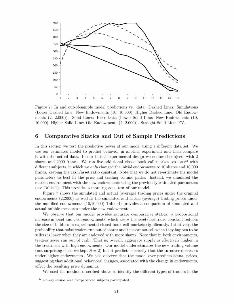
Figure 7: In and out-of-sample model predictions vs. data. Dashed Lines: Simulations(Lower Dashed Line: New Endowments (10, 10.000), Higher Dashed Line: Old Endow-ments (2, 2.000)). Solid Lines: Price-Data (Lower Solid Line: New Endowments (10,10.000), Higher Solid Line: Old Endowments (2, 2.000)). Straight Solid Line: FV.

6 Comparative Statics and Out of Sample Predictions

In this section we test the predictive power of our model using a different data set. Weuse our estimated model to predict behavior in another experiment and then compareit with the actual data. In our initial experimental design we endowed subjects with 2shares and 2000 francs. We ran five additional closed book call market sessions42 withdifferent subjects, in which we only changed the initial endowments to 10 shares and 10,000francs, keeping the cash/asset ratio constant. Note that we do not re-estimate the modelparameters to best fit the price and trading volume paths. Instead, we simulated themarket environment with the new endowments using the previously estimated parameters(see Table 1). This provides a more rigorous test of our model.

Figure 7 shows the simulated and actual (average) trading prices under the originalendowments (2,2000) as well as the simulated and actual (average) trading prices underthe modified endowments (10,10,000) Table 4) provides a comparison of simulated andactual bubble-measures under the new endowments.

We observe that our model provides accurate comparative statics: a proportionalincrease in asset and cash-endowments, which keeps the asset/cash ratio constant reducesthe size of bubbles in experimental closed book call markets significantly. Intuitively, theprobability that noise traders run out of shares and thus cannot sell when they happen to besellers is lower when they are endowed with more shares. Note that in both environments,traders never run out of cash. That is, overall, aggregate supply is effectively higher inthe treatment with high endowments. Our model underestimates the new trading volume(not surprising since we kept S = 2) but it predicts correctly that the turnover decreasesunder higher endowments. We also observe that the model over-predicts actual prices,suggesting that additional behavioral changes, associated with the change in endowments,affect the resulting price dynamics.

We used the method described above to identify the different types of traders in the

42In every session nine inexperienced subjects participated.

21

Table 4: Bubble Measures: Out-of-sample (10,10,000)

. Total Average TrendTurnover Amplitude Dispersion Bias APD PD RAD RD RPAD Haessel Boom Dur.

Data, Mean 1.18 1.56 824 40.53 9.16 6.76 0.29 0.21 0.35 0.87 10 2(Std) (0.39) (0.8) (565.4) (39.3) (6.3) (6.5) (0.2) (0.2) (0.22) (0.2) (1.7) (0.8)

Sim 0.69 2.63 1969 157 23.6 20.4 0.74 0.64 1.06 0.4 14 6

data. That is, we used the average simulated trading strategies stemming from the originalexperimental design (2,2000) to ensure a proper out-of-sample analysis. The session spe-cific type distributions are given in Table 5. Overall, out of the 45 subjects, we identify 11speculators (24%) and 16 fundamental traders (38%) – a distribution quite similar to theone derived under the original design. The simulated terminal wealth levels of fundamentaltraders, speculators and noise traders are 15.434, 13.765 and 12.991 francs respectively.The simulated terminal wealth distribution indicates that fundamental traders earn signi-ficantly more money than speculators and noise traders in this environment. Speculatorsonly make slightly more money than noise traders. This is not that surprising since bubblesare smaller under high endowments, thus implying reduced opportunities for capital gains.Empirically we observe a wealth distribution which is similar to the simulated one: fun-damental traders end up with significantly higher terminal wealth levels than speculatorsat a 1% level (Mann-Whitney test, p-value: 0.005). Fundamental traders make also moremoney than noise traders. The latter difference is significant at a 5% level. The terminalwealth levels of noise traders and speculators are not significantly different at a 5% level(Mann-Whitney p-value: 0.07). Similar to our finding above we observe that the medianwealth levels of speculators, fundamental and noise traders are not significantly differentto the simulated final wealths (p-values: Speculators: 0.67; Fundamental: 0.45; Noise:0.73).We observe again that fundamental traders perform better than noise traders on theCRT at a 10% level (Mann-Whitney p-value: 0.067). The difference between the CRT-performances of fundamental traders and speculators is not significant (p-value: 0.47).Furthermore, speculators and fundamental traders perform jointly better on the CRTthan noise traders at a 10% level (p-value: 0.09).

Table 5: Trader Types Summary Statistics: Out of sample

Sessions Speculators Fundamental Noise

1 22% 44% 34%2 33% 33% 34%3 22% 44% 34%4 11% 33% 56%5 33% 22% 45%

CRT Wealth CRT Wealth CRT Wealth

Median 1.5 12030 2 14305 1 13236Average 1.6 11440 2 14095 1.15 13551Std. Err. (1.35) (1856) (1.08) (812) (1.14) (3750)

Overall, the out-of-sample analysis suggests that our model can be used to investigatehow changes in the environment affect the dynamics of bubble formation. It can also beused to guide the design of policies that may help to dampen or eliminate bubbles.

22

7 Conclusion

This paper provides a heterogeneous agent model for experimental closed-book call-marketswith heterogeneous agents, namely, with speculators, fundamental and noise traders. Weestimate the parameters of the model using experimental data. The model allows us toidentify the different types of traders in the data. We find that fundamental traders andspeculators have both higher cognitive abilities and terminal wealth than noise traders.

Furthermore, we find that all three types of traders are essential to explain the mech-anics of bubbles and crashes. Specifically, fundamental traders buy from noise traders ininitial periods initiating an upward trend in prices. Next, speculators buy from funda-mental traders during the boom. Finally, speculation is only profitable in this environmentdue to the presence of noise traders who are willing to buy the overvalued asset in laterperiods.

Our model can be used to obtain out-of-sample predictions. For instance, it can beused to analyze how changes in the environment (e.g., changes in the dividend and fun-damental value processes, trading institutions, experience level, etc.) affect the dynamicsof bubble formation. It can also be used to guide the design of policies that may helpdampen bubble formation.

References

D. Abreu and M. K. Brunnermeier. Bubbles and crashes. Econometrica, 71:173–204, 2003.

L. F. Ackert, Charupat N., Deaves R., and B. D. Kluger. The origins of bubbles inlaboratory asset markets. Federal Reserve Bank of Atlanta, 6, 2006.

M. Arellano and S. Bond. Some tests of specification for panel data: Monte carlo evidenceand an application to employment equations. Review of Economic Studies, 58:277–297,1991.

R. Blundell and S. Bond. Initial conditions and moment restrictions in dynamic paneldata models. Journal of Econometrics, 87:115–143, 1998.

M.V. Boening, S. LaMaster, and A. Williams. Price bubbles and crashes in experimentalcall markets. Economics Letters, 41:179–185, 1993.

P. Bossaerts, C. Plott, and W. R. Zame. Prices and portfolio choices in financial markts:theory, econometrics, experiments. Econometrica, 75(4):993–1038, 2007.

M. Brunnermeier. Bubbles. New Palgrave Dictionary of Economics, 2008.

M. K. Brunnermeier and L. H. Pedersen. Predatory trading. Journal of Finance, 60:1825–1863, 2005.

R.H. Byrd, M. C. Hribar, and J. Nocedal. An interior point algorithm for large-scalenonlinear programming. SIAM Journal on Optimization, 9:877–900, 1999.

R.H. Byrd, J. C. Gilbert, and J. Nocedal. A trust region method based on interior pointtechniques for nonlinear programming. Mathematical Programming, 89:149–185, 2000.

G. Caginalp and V. Ilieva. The dynamics of trader motivations in asset bubbles. Journalof Economic Behavior and Organization, 66(3 – 4):641–656, 2005.

23

G. Caginalp and H. Merdan. Asset price dynamics with heterogeneous groups. PhysicaD, 225:43–54, 2007.

G. Caginalp, D. Porter, and V. Smith. Momentum and overreaction in experimental assetmarkets. International Journal of Industrial Organization, 18:80–99, 2000.

G. Caginalp, D. Porter, and V. Smith. Financial bubbles: Excess cash, momentum andincomplete information. The Journal of Psychology and Financial Markets, 2(2):80–99,2001.

C. F. Camerer, T-H. Ho, and J-K. Chong. A cognitive hierarchy model of games. TheQuarterly Journal of Economics, 119:861–898, 2004.

T. Cason. Call market efficiency with simple adaptive learning. Economics Letters, 40:27–32, 1992.

M. A. Costa-Gomes and V. P. Crawford. Cognition and behavior in two-person guessinggames: An experimental study. American Economic Review, 96(2):1737–1768, 2006.

V. P. Crawford and N. Iriberri. Level-k auctions: Can a non-equilibrium model of stra-tegic thinking explain the winner’s curse and overbidding in private-value auctions?Econometrica, 75(6):1721–1770, 2007.

V. P. Crawford, M. A. Costa-Gomes, and N. Iriberri. Structural models of nonequilibriumstrategic thinking: Theory, evidence and applications. Journal of Economic Literature,51, 2013.

D. M. Cutler, J. M. Poterba, and L. H. Summers. Speculative dynamics and the role offeedback traders. American Economic Review, 80:63–68, 1990.

R. Davidson and J. MacKinnon. Several tests for model specification in the presence ofalternative hypotheses. Econometrica, 49:781–793, 1981.

J. B. DeLong, A. Shleifer, L. H. Summers, and R. J. Waldman. Positive feedback invest-ment strategies and destabilizing rational speculation. Journal of Finance, 45:379–395,1990a.

J. B. DeLong, A. Shleifer, L. H. Summers, and R. J. Waldmann. Trader risk in financialmarkets. Journal of Political Economy, 98:703–738, 1990b.

J. Duffy. Agent-Based Models and Human Subject Experiments, in: L. Tesfatsion andK.L. Judd, eds., Handbook of Computational Economics Vol. 2 Handbooks in EconomicsSeries. Elsevier/North-Holland (Handbooks in Economics Series), 2006.

J. Duffy and U. M. Unver. Asset price bubbles and crashes with near-zero-intelligencetraders. Economic Theory, 27:537–563, 2006.

M. Dufwenberg, T. Lindqvist, and E. Moore. Bubbles and experience: An experiment.American Economic Review, 95(5):1731–1737, 2005.

U. Fischbacher. Z-tree: Zurich toolbox for ready-made economic experiments. Experi-mental Economics, 10(2):171–178, 2007.

S. Frederick. Cognitive reflection and decision making. Journal of Economic Perspectives,19:25–42, 2005.

24

M. Gladwell. The Tipping Point: How Little Things Can Make a Big Difference. BackBay Books, 2002.

D. K. Gode and S. Sunder. Allocative efficiency of markets with zero-intelligence traders:Market as a partial substitute for individual rationality. Journal of Political Economy,101(1):119–137, 1993.

O. D. Hart and D. M. Kreps. Price destabilizing speculation. Journal of Political Economy,94:927–633, 1986.

E. Haruvy and C. N. Noussair. The effect of short selling on bubbles and crashes inexperimental spot asset markets. Journal of Finance, 61(3):1119–1157, 2006.

E. Haruvy, Y. Lahav, and C. N. Noussair. Traders’ expectations in asset markets: Exper-imental evidence. American Economic Review, 97(5):1901–1920, 2007.

D. Hirshleifer. Investor psychology and asset pricing. Journal of Finance, 56:1533–1597,2001.

C. Hommes. The heterogeneous expectations hypothesis: Some evidence from the lab.Journal of Economic Dynamics and optimal control, 4:35–64, 2010.

C. Hommes, J. Sonnemans, and J. Tuinstra. Coordination of expectations in asset pricingexperiments. Review of Financial Studies, 18:955–980, 2005.

C. Hommes, J. Sonnemans, J. Tuinstra, and H. van de Velden. Expectations and bubblesin asset pricing experiments. Journal of Economic Behavior and Organization, 67:116–133, 2008.

R. N. Hussam, D. Porter, and V. L. Smith. Thar she blows: Can bubbles be rekindledwith experienced subjects? American Economic Review, 98(3):924–937, 2008.

S. Johansen. Estimation and hypothesis testing of cointegration vectors in gaussian vectorautoregressive models. Econometrica, 59(6):1551–1580, 1991.

R. King, V. Smith, A. Williams, and M. v. Boening. Nonlinear Dynamics and EvolutionaryEconomics. Oxford University Press, 1993.

M. Kirchler and J. Huber. The impact of instructions and procedure on reducing confusionand bubbles in experimental asset markets. Experimental Economics, 102, 2011.

M. Kirchler, J. Huber, and T. Stoeckl. Thar she bursts: Reducing confusion reducesbubbles. American Economic Review, 102(2), 2012.

V. Lei and F. Vesely. Market efficiency: Evidence from a no-bubble asset market experi-ment. Pacific Economic Review, 14(2):246–258, 2009.

V. Lei, C. N. Noussair, and C. R. Plott. Nonspeculative bubbles in experimental asset mar-kets: Lack of common knowledge of rationality vs. actual irrationality. Econometrica,69(1):831–859, 2001.

V. Lugovskyy, D. Puzzello, and S. Tucker. An experimental study of bubble formation inasset markets using the tatonnement trading institution. 2011.

S. Moinas and S. Pouget. The bubble game: An experimental study of speculation.forthcoming: Econometrica, 2012.

25

R. Nagel. Unraveling in guessing games: An experimental study. American EconomicReview, 85:1313–1326, 1995.

R. Nagel and J. Duffy. On the robustness of behaviour in experimental beauty contestgames. The Economic Journal, 107:1684–1700, 1997.

R. Nagel and B. Grosskopf. The two-person beauty contest. Games and Economic Beha-vior, 62:91–99, 2008.

D. Porter and V. L. Smith. Futures markets and dividend uncertainty in experimentalasset markets. Journal of Business, 68(4):509–541, 1995.

V. Smith, G. L. Suchanek, and A. Williams. Bubbles, crashes, and endogenous expecta-tions in experimental spot asset markets. Econometrica, 56(5):1119–1151, 1988.

V. Smith, M. v. Boening, and C. Wellford. Dividend timing and behavior in laboratoryasset markets. Economic Theory, 16(3):567–583, 2000.

D. O. Stahl and P. Wilson. Experimental evidence on players’ models of other players.Journal of Economic Behavior and Organization, 25:309–327, 1994.

D. O. Stahl and P. Wilson. On players’ models of other players: Theory and experimentalevidence. Games and Economic Behavior, 10:218–254, 1995.

R. A. Waltz, J. L. Morales, J. Nocedal, and D. Orban. An interior algorithm for nonlinearoptimization that combines line search and trust region steps. Mathematical Program-ming, 107:391–408, 2006.

A. Williams. The formation of price forecasts in experimental markets. Journal of Money,Credit, and Banking, pages 1–18, 1987.

A. Williams. Price Bubbles in Large Financial Asset Markets? Handbook of ExperimentalEconomics Results, 2008.

8 Appendix A

The Frederick cognitive reflection test consists of the following three questions (answersin brackets):

• A bat and a ball cost $1.10 in total. The bat costs $1 more than the ball. How muchdoes the ball cost? (5)

• If it takes five machines five minutes to make five widgets, how long would it take100 machines to make 100 widgets? (5)

• In a lake, there is a patch of lily pads. Every day, the patch doubles in size. If ittakes 48 days for the patch to cover the entire lake, how long would it take for thepatch to cover half the lake? (47)

Frederick (Frederick [2005]) shows that the number of correct answers on the previousthree questions are positively correlated with subject-specific results on other cognitiveability tests such as the Wonderlic Personnel Test (WPT)43 and the “need for cognition

43A 12-minute, 50-item test used by the National Football League and other employers to assess theintellectual abilities of their prospective hires.

26

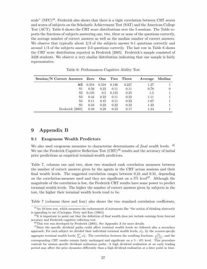
scale” (NFC)44. Frederick also shows that there is a tight correlation between CRT scoresand scores of subjects on the Scholastic Achievement Test (SAT) and the American CollegeTest (ACT). Table 6 shows the CRT score distributions over the 5 sessions. The Table re-ports the fractions of subjects answering one, two, three or none of the questions correctly,the average number of correct answers as well as the median number of correct answers.We observe that typically about 2/3 of the subjects answer 0-1 questions correctly andaround 1/3 of the subjects answer 2-3 questions correctly. The last row in Table 6 showsthe CRT score distribution reported in Frederick [2005]. Frederick’s sample consisted of3428 students. We observe a very similar distribution indicating that our sample is fairlyrepresentative.

Table 6: Performances Cognitive Ability Test

Session/N Correct Answers Zero One Two Three Average Median

All 0.318 0.318 0.136 0.227 1.27 1S1 0.56 0.22 0.11 0.11 0.78 0S2 0.125 0.5 0.125 0.25 1.5 1S3 0.44 0.22 0.11 0.22 1.11 1S4 0.11 0.45 0.11 0.33 1.67 1S5 0.34 0.22 0.22 0.22 1.33 1

Frederick [2005] 0.33 0.28 0.23 0.17 1.24 1

9 Appendix B

9.1 Exogenous Wealth Predictors

We also used exogenous measures to characterize determinants of final wealth levels. 45

We use the Frederick Cognitive Reflection Test (CRT)46 results and the accuracy of initialprice predictions as empirical terminal-wealth predictors.

Table 7, columns one and two, show two standard rank correlation measures betweenthe number of correct answers given by the agents in the CRT across sessions and theirfinal wealth levels. The suggested correlation ranges between 0.24 and 0.31, dependingon the correlation-measure used and they are significant on a 5% level47. Although themagnitude of the correlation is low, the Frederick CRT results have some power to predictterminal wealth levels. The higher the number of correct answers given by subjects in thetest, the higher their terminal wealth levels tend to be.

Table 7 (columns three and four) also shows the two standard correlation coefficients,

44An 18-item test, which measures the endorsement of statements like “the notion of thinking abstractlyis appealing to me (Cacioppo, Petty and Kao (1984))

45It is important to point out that the definition of final wealth does not include earnings from forecastaccuracy and Frederick cognitive reflection test.

46This test was developed by Frederick (2005). See Appendix A for more details.47Since the specific dividend paths could affect terminal wealth levels we followed also a secondary

approach: For each subject we divided their individual terminal wealth levels, xiT , by the session-specific

aggregate terminal wealth levels,∑i x

iT . The correlation between the resulting fractions,

xiT∑i x

iT

, and the

corresponding CRT results remain fairly unchanged and significant on a 5 - 6% level. This procedurecontrols for session specific dividend realization paths: A high dividend realization at an early tradingperiod may affect the price dynamics differently than a high dividend realization at a later point in time.

27

measuring the relationship between the terminal wealth level of subjects across exper-iments and a prediction-accuracy measure. The prediction accuracy measure for everysubject is computed as the absolute value of the difference between the price prediction ofevery individual in period 1 and the fundamental value of the asset in period 1. Similarlyone could use the realized price in period 1 as a benchmark to evaluate the accuracy of theprice prediction in period 1. The analogous results using the period one prices as bench-mark are shown in columns five and six. The results indicate that both the Kendall andthe Spearman correlation measures are significant and negative on a 5% level. The res-ults are intuitive: better initial price predictions, reflecting a better understanding of theinstructions and the market environment, result in higher terminal wealth levels.48 The

Table 7: Terminal Wealth Predictors*

Correlation between Terminal Wealth and...Correct Answers |Prediction1 − FV1| |Prediction1 − P1|

Kendall Spearman Kendall Spearman Kendall Spearman

0.24 0.31 -0.22 -0.33 -0.21 -0.30(0.04) (0.04) (0.04) (0.03) (0.05) (0.05)

*P-values in parentheses

two previous results indicate that both the CRT results and initial price forecast accuracymeasures are suitable empirical predictors for terminal wealth levels. This suggests thatthe initial price forecast accuracy and the number of correct answers should also show asignificant and negative correlation. Table 8 provides support for this conjecture. Indeedthe correlation is significant on a 1% level indicating that the accuracy of the initial priceprediction and the Frederick CRT elicit cognitive abilities of subjects on a similar qualitylevel.

Table 8: Correlation correct answers and prediction accuracy in period 1*

Kendall SpearmanCorr. (# Correct Answers, |Prediction1 − P1|) -0.38 -0.47

(< 0.01) (< 0.01)

Corr. (# Correct Answers, |Prediction1 − FV1|) -0.38 -0.48(< 0.01) (< 0.01)

*P-values in parentheses

10 Appendix C

To perform the J-test we ran the following regressions:

(SFN) : pEt = β0 + β1pt + ε1t

(NZI) : pEt = β0 + β1pt + ε2t ,

where pEt is the average observed price in period t, pt is the period t’s price stemming fromthe simulations which includes speculators, fundamental and noise traders (SFN) , and ptis the period t’s price stemming from the simulations which includes only NZI traders as

48Similar to the procedure used for the previous Table we re-calculated the correlations using the session-wide normalized terminal wealth levels as an experimental performance measure. This procedure preservesthe significance on a 5% level.

28

in Duffy and Unver [2006]. The fit of SFN specification, measured via R2, exceeds the fitof the NZI specification (94% versus 79%). However, a direct comparison via the R2’s isnot possible since the models are not nested. We therefore conducted a standard J-testfor non-nested models, following Davidson and MacKinnon [1981], to decide between thetwo specifications. Controlling for heteroscedasticity we can reject the NZI specificationin favor of the SFN specification (our model) at a 1% level (p-value = 0.007).

11 Appendix D: Individual Behavior: DeLong et al. [1990a]

In what follows, we analyze our data through the lenses of the well-established model ofDeLong et al. [1990a] (DSSW) as applied to experimental markets by Haruvy and Noussair[2006] (HN). The main point is to show that our model provides a better framework tounderstand the data than the DSSW model. DSSW present a heterogeneous agent modelconsisting of trend-chasers or feedback traders, fundamental or passive traders and rationalspeculators. 49

Following DSSW and Haruvy and Noussair [2006] (HN), the functional forms of the de-mand functions, D(.), of trend chasers (feedback traders), fundamental or passive traders(FV traders) and speculators are given in equations (12), (13) and (14) respectively:

D(pt−1, pt−2) = −δ + β(pt−1 − pt−2) (12)

D(pt) = −α(pt − FVt) (13)

D(pt+1, pt) = γ(E(pt+1)− pt) (14)

where δ, β, α and γ are all non-negative parameters, E(.) is the expectations-operator, FVtis the fundamental value of the asset in period t, and pt is the uniform transaction pricein period t.

We use exactly the same method as HN to classify every subject (for every sessionseparately) into one of the three types. For instance, if the change in a subjects’ assetholdings does not have the opposite sign as the difference of the transaction prices inperiod t − 1 and t − 2, that subject is classified as a trend-chaser for that particularperiod. Similarly, if the difference between the fundamental value of the asset in period tand the transaction price in period t does not have the opposite sign as the change in asubjects’ asset holdings in period t, he or she is classified as fundamental trader in periodt. Lastly, a subject is classified as speculator in period t if the difference between theaverage transaction price in period t+1 and the average transaction price in period t doesnot have the opposite sign as the change in a subjects’ asset holdings for that period.50

Finally, the number of periods in which each subject belongs to every single type arecounted, yielding a vector of three scores for every participant. A subject is classified asagent of the type for which he has the highest score, provided that the score is greaterthan or equal to τ = 8. If a subject has a maximum score lower than 8, that subject doesnot belong to any of the three types and is classified as “other”. If a subject’s maximumscore is the same for two (three) types and is higher than 8, the participant is assigned aweight of 1/2 (1/3) to each type for which he has the same maximum score.

When applying this approach to our data ?0.337 0.394 0.269 0 we obtain the overalltype distributions very similar to the trader type distributions in Table VI of Haruvy

49Their model provides a theoretical framework to investigate the potential consequences of destabilizingrational speculation in financial markets. For similar and additional follow up contributions see also Hartand Kreps [1986], DeLong et al. [1990b], Cutler et al. [1990], Hirshleifer [2001], Abreu and Brunnermeier[2003], Brunnermeier and Pedersen [2005]).

50Note that speculators are assumed to have perfect foresight.

29

and Noussair [2006]. Namely we identify 33.7% of subjects as Passive traders, 39.4% asFeedback traders, 26.9% as Speculators, and 0% as Others.

Next, we discuss the robustness of the trader type classifications mentioned abovewhen a notion of statistical significance is introduced.

As a motivating example for doing so, consider a session in which prices increase inevery period and remain above the fundamental value in the last period. Further, considera subject who neither buys nor sells assets in T −1 periods but sells some shares in periodT . Based on the method of HN, the subject would be equally classified as speculator,passive trader and feedback trader in T − 1 of the T periods. Since the subject in ourexample sells in period T –prices were rising in every period and exceed the fundamentalvalue– he would be classified as a passive trader in the last period. In other words, althoughthat participant’s classification is ambiguous for T − 1 out of T periods, the scoring rulepresented by HN would still uniquely assign the subject into the fundamental trader typeclass.

To address this concern and to examine the robustness of the classification rule presen-ted by HN, we test the correlations between changes in individual asset holdings and therelevant price/fundamental value differences.

For instance, if there is significant positive correlation between changes in trader i’sasset holdings and the difference between fundamental values and prices in every period,we cannot reject the null hypothesis that trader i is a fundamental trader. Similarly,if there is significant positive correlation between changes in trader i’s asset holdingsand the difference between prices in period t − 1 and period t − 2, we cannot reject thenull hypothesis that trader i is a feedback trader. Lastly, if there is significant positivecorrelation between changes in trader i’s asset holdings and the differences between pricesin period t + 1 and period t, we cannot reject the null hypothesis that trader i is aspeculator. Whenever we cannot reject that a subject belongs to more than one type, theparticipant is assigned equal weight to each type he may belong to. Like before, whenever aparticipant does not belong to any of three types –either because there is no positive or nosignificant correlation– we classify him as “other”. This approach is a natural extension ofthe method described by HN and introduces a notion of significance into their framework.

For every session and participant we compute non-parametric Spearman-correlations51

between changes in individual asset holdings and the relevant price/fundamental value dif-ferences at varying significance levels. The resulting trader type distributions are presentedin the lower panel of Table 9 (Method III).

Imposing a significance level of 5%, we observe that the method of HN significantlyclassifies around 16% of all traders into one of the three types, whereas 84% are classifiedas “other”. Even after relaxing the significance level to 25%, only 32% of all traders canbe classified into one of the three trader-types, whereas 68% remain “others”. Lastly, weobserve that the smallest fraction of traders are fundamental traders, independently of thesignificance level imposed.

The robustness concerns and fairly large unexplainable behavioral components are notthe only reasons why we present an alternative method to identify different trader typesin the following sections.

Another reason is the difference in institutional frameworks. While HN classify theirparticipants into DSSW-types under a double auction trading environment, we consider aclosed book call market.

To clarify why trading institutions may matter in this context, consider the classifica-tion of fundamental or passive traders. In the model of DSSW, passive traders buy assets

51We also compute Kendall-correlations but the results discussed below change only marginally.

30

Table 9: Trader Type Classification based on DeLong et al. [1990a] and Haruvy andNoussair [2006]

Passive Feedback Speculators Others Passive Feedback Speculators Others

Method: Haruvy & Noussair I (Dropping first two periods and last)τ: 8 τ: 9

Distribution 0.364 0.295 0.341 0 0.364 0.284 0.330 0.023CRT Average 1.200 1 1.556 1.200 1 1.556 0CRT Median 1 1 2 1 1 2 0

τ: 10 τ: 11

Distribution 0.330 0.284 0.318 0.068 0.277 0.186 0.220 0.318CRT Average 1.222 1 1.556 0.333 1.250 1.400 1.667 0.857CRT Median 1 1 2 0 1 1 2 0.500

Method: Haruvy & Noussair II (Including first two periods and last)τ: 8 τ: 9

Distribution 0.337 0.394 0.269 0 0.337 0.394 0.269 0CRT Average 1.222 0.833 1.286 1.222 0.833 1.286CRT Median 1 1 1 1 1 1

τ: 10 τ: 11

Distribution 0.337 0.394 0.269 0 0.326 0.383 0.269 0.023CRT Average 1.222 0.833 1.286 1.212 0.793 1.236 1CRT Median 1 1 1 1 1 1 1

Method: Haruvy & Noussair III (Significance test; Including first two periods and last)level = 0.05 level = 0.10

Distribution 0.023 0.068 0.068 0.841 0.045 0.091 0.068 0.795CRT Average 1 1 1.333 1.297 0.500 1 1.333 1.343CRT Median 1 1 1 1 0.500 1 1 1

level = 0.15 level = 0.25

Distribution 0.045 0.091 0.091 0.773 0.068 0.160 0.09 0.681CRT Average 0.500 1 1 1.382 0.333 1 1 1.467CRT Median 0.500 1 0.500 1 0 1 0.500 1

whenever the fundamental value in period t exceeds the price in period t. However, undera closed book call market the period t transaction price is ex-ante unobservable.

As a matter of fact, in a closed book call market, passive traders would have toform expectations about transaction prices in period t, before they submit their limitorders. The HN-classification-method approximates individual expectations by actualtrading prices, assuming that passive traders have perfect foresight. The same argumentholds for speculators, whose expectations about transaction prices in period t+ 1 are alsoapproximated by actual transaction prices. Put differently, while rational expectationsmay be a good approximation for actual expectations under double auctions, it might bea worse approximation for closed book call markets.52

11.1 DeLong et al. [1990a]+ε

In this section we provide additional evidence, showing that the DSSW model and its ad-apted version presented by Haruvy and Noussair [2006] does not generate price processes,which fit our data.

To address goodness of fit questions, we first estimate the type distribution and theassociated demand parameters following the method of HN. HN estimate the type distri-bution and the demand parameters by minimizing the root mean square error (RMSE)between average session- and simulated prices stemming from their model.

Simulating prices based on the demand functions in (12), (13) and (14) requires someassumptions on the expectation formation process of speculators. HN solve this potentialissue in their RMSE-minimziation algorithm via a level-k model structure,53 assumingthat speculators form expectations in two steps:

52There is plenty of evidence that the rational expectations hypothesis does not hold in laboratory assetmarkets with uniform market clearing prices (Hommes et al. [2005, 2008], Hommes [2010]).

53See Nagel [1995], Nagel and Duffy [1997], Camerer et al. [2004], Nagel and Grosskopf [2008], Crawfordand Iriberri [2007], Crawford et al. [2013].

31

In the first step, speculators believe that the price in period t + 1 equals the funda-mental value. Based on this prior, speculators compute the resulting equilibrium pricesfor each period, taking their own price effect into account. In the second step, speculatorsuse the resulting price-sequence as their price expectations for every period.

Before we use the method of HN and present our estimation results, we device asimple statistical test to check whether our data is indeed generated by a model, which isconsistent with the assumptions of DSSW and HN.

Following the approach of Bossaerts et al. [2007], who present a CAPM+ε model, wefirst rewrite the demand functions in (12), (13) and (14) as:

Di,t(.) = Di,t(.) + εi,t,

where i represents one of the three types from above. We add a mean-zero-noise-term,εi,t, to the demand functions of every type, capturing random factors which may affectindividual demands. Along the lines of Bossaerts et al. [2007], we assume that these noiseterms are identically and independently distributed (iid) over time but not necessarilyacross types.

Next, letting N1, N2 and N3 be the fractions of feedback traders, passive traders andspeculators respectively (which sum to one), we compute the equilibrium prices as:

pt =N1δ

N2α+N3γ+

N2α

N2α+N3γFVt +

N3γ

N2α+N3γEpt+1 (15)

− N1β

N2α+N3γpt−1 +

N1β

N2α+N3γpt−2 + f(ε1,t, ε2,t, ε3,t),

where f(ε1,t, ε2,t, ε3,t) is a mean zero, iid random noise term. Using the belief formationstructure of HN, the first step equilibrium prices are

pt =N1δ

N2α+N3γ+

N2α

N2α+N3γFVt +

N3γ

N2α+N3γFVt+1 (16)

− N1β

N2α+N3γpt−1 +

N1β

N2α+N3γpt−2 + f(ε1,t, ε2,t, ε3,t)

Using the observation that in experimental asset markets the fundamental value de-creases in every period by the average dividend-payment, d,54 iterating (16) one periodforward and taking expectations, we obtain the following level-1 expectations for specu-lators:

Ept+1 = FVt +N1δ −N3γd

N2α+N3γ− d+

N1β

N2α+N3γ(pt−1 − pt) (17)

Plugging (17) into (15) and collecting terms yields a price process of the form:

pt = m0 +m1FVt +m2pt−1 +m3pt−2 + ηt, (18)

where

m0 =1

1 + N3γN1β(N2α+N3γ)2

1

N2α+N3γ[N1δ +N3γ(

N1δ −N3γd

N2α+N3γ− d)],

m1 =1

1 + N3γN1β(N2α+N3γ)2

,

54I.e.: FVt+k = FVt − dk.

32

m2 =1

1 + N3γN1β(N2α+N3γ)2

N1β(N3γ

N2α+N3γ− 1),

m3 =N1β

1 + N3γN1β(N2α+N3γ)2

,

and ηt is an iid noise term with mean zero. Based on the non-negativity constraints onthe parameters in the models of DSSW and HN, the coefficient m2 has to be non-positive,whereas the coefficient m3 has to be non-negative. In summary the validity of the set ofassumptions, imposed by DSSW and HN can be tested via the following null hypotheses:

H0 : m2 ≤ 0,m3 ≥ 0 (19)

To test (19) we take first differences of the variables in (18) and estimate the coefficientsm2 and m3 via standard dynamic panel methods.55

Columns (4) and (5) of Table 10 show the Arellano-Bond56 (AB) and Blundell-Bond57

(BB) estimates for m2 and m3 respectively. Note that for the AB estimates we can rejectthat m2 is non-positive whereas for the BB-estimates we can reject that m3 is non-negative(5% significance level).58

Since we can reject the joint hypothesis in (19), we conclude that the DSSW modeldoes not generate price sequences, which are consistent with our data.

To investigate why the DSSW model does not fit our data, we estimate the struc-tural parameters of the model, following the method presented in HN.59 The parameterestimates and the type distributions are shown in the first row of Table 11.

Note that the estimates indicate that α equals zero, rendering the actual fractionof fundamental traders, which are supposed to have rational expectations about tradingprices in period t, unidentifiable. Moreover, since the fractions of all other trader typesdepend on the estimated fractions of fundamental traders, their relative proportions arenot identifiable either.

In a second estimation step we therefore dropped passive traders, whose behavior –as specified in the models of DSSW and HN– does not seem to contribute to our datagenerating process. The resulting estimates are shown in the second row of Table 11.However, this partial identification strategy is problematic, since the model of DSSWrequires all three trader types for the emergence of bubbles.

Put differently, we know that we are missing at least one relevant type so that ourobserved bubbles emerge but we don’t know its relative proportion or how the type actuallybehaves. Nevertheless, we can assert that out of the identifiable traders, around 72% arefeedback traders and about 28% are speculators (second row of Table 11).

Our results –based on aggregate data– suggest that there are no participants in oursubject pool who can be identified as fundamental traders with rational expectations.Note that this finding is consistent with our results from Method III in Table 9. There,we show that among all three trader classes the fraction of fundamental traders is alwaysthe smallest. To further investigate that it is the lack of FV traders, which is responsiblefor rejecting the DSSW model for our data, we re-estimate the parameters along the linesof HN, fixing the trader type distribution.

55Note that the first difference of FV is constant and therefore dropped from the estimation.56See Arellano and Bond [1991].57See Blundell and Bond [1998].58Columns (1) - (3) show the fixed effect, random effects and between estimates for m2 and m3 respect-

ively.59We minimize the RMSE using Byrd et al. [1999, 2000], Waltz et al. [2006].

33

We use the trader type distribution under Method I, with τ = 8 from Table 9 – whichcorresponds to the method used by HN– but mention that other trader type distributionsfrom the same Table yield similar result. The estimation results for the demand paramet-ers, restricting the type distributions, are shown in the third row of Table 11. Note thatthe optimal α is again estimated to be zero, which is simply another way of setting theeffect of FV traders to zero in the model.

Table 10: Testing DeLong et al. [1990a]+ε

(1) (2) (3) (4) (5)Random Effects Fixed Effects Between Arellano, Bond Blundell, Bond

m2 0.401∗∗ 0.402∗∗ 0.0742 0.502∗∗ -0.221∗

(0.026) (0.000) (0.864) (0.010) (0.053)

m3 -0.00425 0.000358 0.534 -0.0603 -0.259∗∗

(0.945) (0.995) (0.296) (0.529) (0.026)

N 68 68 68 59 63

p-values in parentheses

∗ p < 0.10, ∗∗ p < 0.05

Table 11: Estimation Results; Method: Haruvy and Noussair [2006] (Minimizing RMSE).

α γ δ β N1 N2 N3

0 0.4182 5.9224 0.0228 0.4878 0.4608 0.0514- 0.1476 7.4101 0.0268 0.7282 - 0.27180 0.0643 7.4871 0.0288 0.364 0.295 0.341

In summary, we conclude that the model of DSSW and its adapted version presentedby HN does not generate prices, which are consistent with our data. We identify thelack of FV-traders with rational expectations about period t trading prices as one of thereasons, why we can reject the model of DSSW and HN in favor of potential alternatives.

34