Trade Reform and Poverty in the Philippines: A Computable General Equilibrium Microsimulation Analysis 1

Caesar B Cororaton and John Cockburn2

Abstract

The paper employs an integrated CGE-microsimulation approach to analyze the poverty effects of tariff reduction. The results indicate that the tariff cuts implemented between 1994 and 2000 were generally poverty-reducing, primarily through the substantial reduction in consumer prices they engendered. However, the reduction is much greater in the National Capital Region (NCR), where poverty incidence is already lowest, than in other areas, especially rural, where poverty incidence is highest. Tariff cuts lower the cost of local production and bring about real exchange rate depreciation. Since the non-food manufacturing sector dominates exports in terms of export share and export intensity, the general equilibrium effects of tariff reduction is an expansion of this sector and a contraction in the agricultural sector. This, in turn, leads to an increase in the relative returns to factors, such as capital, used intensively in the non-food manufacturing sector and a fall in returns to unskilled labor. As rural households depend more on unskilled labor income, income inequality worsens as a result. Keywords: computable general equilibrium, microsimulation, international trade, poverty, Philippines JEL: D33, D58, E27, F13, F14, I32, O15, O53

1This research was done with financial support from the International Development Research Centre (IDRC) under the project Micro Impacts of Macro Adjustment Policies (MIMAP). 2Philippine Institute for Development Studies (ccororaton@mail.pids.gov.ph) and Laval University (jcoc@ecn.ulaval.ca)

1

1. Introduction

One of the first major reforms implemented in the Philippines was in the foreign trade sector. Since its first major reform in the early 1980s, significant changes have taken place: Tariff rates have been reduced, the tariff structure simplified, and quantitative restrictions “tariffied”. However, the impact of these reforms on the poor is not very clear. In fact, it is a subject of very intense debate. Do the poor share in the gains from freer trade? What alternative or accompanying policies may be used in order to ensure a more equitable distribution of the gains from freer trade? What are the transmission mechanisms through which these reforms may affect the poor? These are examples of very challenging policy issues that occupy the ongoing debate on trade reforms. Given the economy-wide nature of trade reform, it is usually analyzed in the context of a computable general equilibrium (CGE) model that is calibrated to national accounting data. In contrast, given the ir nature, poverty issues are generally examined using individual or household data. In this paper, we attempt to put these two approaches together in an integrated CGE-microsimulation model to examine the poverty effects of trade reforms in the Philippines. In particular, we construct a standard CGE model, calibrated to 1994 ("pre-reform") Philippine data, in which we integrate all 24,979 households from the 1994 Family Income and Expenditure Survey (FIES) in order to capture the specific impacts on each household. 2. Survey of Literature

There have been numerous attempts to adapt CGE models to the analysis of income distribution and poverty issues. The simplest approach is to increase the number of categories of households and examine how different types of households (rural vs. urban, landholders vs. sharecroppers, region A vs. region B, etc.) are affected by a given shock. However, nothing can be said about the relative impacts on households within any given category because the model only generates information on the representative (or "average") household. There is increasing evidence that households within a given category may be affected quite differently according to their asset profiles, location, household composition, education, etc. Although this problem of intra-category variation may decrease with greater disaggregation of household categories, for example in the work of Piggott and Whalley (1985) where over 100 household categories were considered, one still has to impose strong assumptions concerning the distribution of income among households within each category in order to conduct the conventional poverty and income distribution analysis.

A popular approach is to assume a lognormal distribution of income within each category where the variance is estimated with the base year data (De Janvry, Sadoulet, and Fargeix, 1991). In this approach, the change in income of the representative household in the CGE model is used to estimate the change in the average income for each household category, while the variance of this income is assumed fixed. Decaluwé et al (2000) argue that a beta distribution is preferable to other distributions such as the lognormal because it can be skewed left or right and thus may better represent the types of intra-category income distributions commonly observed. Cockburn et al. (2004) use the actual incomes from a household survey, rather than assume any given functional form, and apply the change in income of the representative household in the CGE model to each individual household in that category.

Regardless of the distribution chosen, one must further assume that all but the first moment is fixed and unaffected by the shock analyzed. This assumption is hard to defend given the heterogeneity of income sources and consumption patterns of households even within very disaggregated categories. Indeed, it is often found that intra-category income variance amounts to more than half of total income variance.

2

The alternative approach is to model each household individually. As demonstrated by Cockburn (2001) , this poses no particular technical difficulties because it involves constructing a standard CGE model with as many household categories as there are households in the household survey providing the base data.

An independent strand of literature performs such individual-level analysis of macro shocks in partial equilibrium framework. This is commonly referred to as micro-simulations. This literature traces back its origins to the papers of Orcutt (1957 and 1961). More recently, some authors have developed micro-simulation models using household surveys to study issues of income distribution (Bourguignon, Fournier and Gurgand, 2000). However, these models are not in a general equilibrium framework and are thus inappropriate for studying major policy changes, such as trade liberalization, which have important feedback effects.

Some authors – e.g. Savard (2004) – have applied price variations generated by a standard CGE

model to this type of microsimulation model. Savard (2004) has taken this approach further by creating a loop between a CGE model and a microsimulation model in order to ensure that their results are coherent. This approach has the advantage of easily incorporating quite sophisticated specifications, including regime-switching, within the microsimulation model.

Decaluwé, Dumont and Savard (1999) present an integrated CGE micro-simulation model, in

which 150 households are directly modeled within a CGE model, using fictional data from an archetypal developing country. They construct the model to allow comparisons with the earlier approaches with multiple household categories and fixed intra-category income distributions. They show that intra-category variations are important, at least in this fictional context.

General equilibrium micro-simulation analyses utilizing true data are presented in the papers of Tongeren (1994), Cogneau (1999), Cogneau and Robillard (2000), and Cockburn (2001). Tongeren models individual firms, rather than the individual households. Cogneau's analysis focuses on a particular city, Antananarivo, rather than a nation, and on issues concerning primarily labor market. In Cogneau and Robillard, the impact of various growth shocks, such as increases in total factor productivity, on poverty and income distribution is examined in the context of a national model of Madagascar. In particular, they find that "a lthough mean income and price changes are significant, the impact of the various growth shocks on the total indicators of poverty and inequality appears relatively small". They also show that neglect of general equilibrium effects, as in standard micro-simulations, and the assumption of a fixed intra-group income distribution, as in standard CGE models, both create a strong bias in the results. However, the disaggregation of the household account in their model is obtained at the cost of sectoral disaggregation of production. Their model distinguishes only five factors of production and three sectors. As the poverty and income distribution effects of macroeconomic shocks are mediated primarily by differences in household income and consumption patterns, this level of aggregation fails to capture many of the intra-household differences.

Finally, Cockburn examines the impact of trade liberalization on poverty in Nepal using a model that maintains the characteristics of a standard CGE model, but integrates the 3,373 households from a national survey. The household disaggregation is obtained without sacrificing the disaggregation of factors, branches and products required to capture the links between trade liberalization and household-level welfare. In particular, the CGE model incorporates 45 separate sectors of production (15 sectors in three regions) with quite different initial tariff rates. The model also includes 15 separate factors of production: skilled and unskilled labor, agr icultural and non-agricultural capital, and land, all broken down into the three regions. Since the household survey data used provides household information on

3

income from each of the factors and on consumption of each of the 15 goods produced by the branches of production, the links between trade liberalization and household welfare are adequately captured.

In this paper, we closely follow the method developed in Cockburn (2001) and apply the analysis to examine the poverty effects of tariff reduction in the Philippines from 1994 to 2000. In particular, the CGE model is calibrated to Philippine data in 1994 and includes eight factors of production, 12 sectors and all of the 24,797 households from the 1994 FIES. 3. Philippine Trade Reform

The first phase of the trade reform program (TRP) started in the early 1980s with three major components: (a) the 1981-85 tariff reduction; (b) the import liberalization program (ILP); and (c) the complimentary realignment of the indirect taxes. There was a narrowing of the structure of tariff rates from the 100 – 0 percent range to 50 – 10 percent. During the period 1983–1985 sales taxes on imports and locally produced goods were equalized. The mark–up applied on the value of imports (for sales tax valuation) was also reduced and eventually eliminated.

The implementation of ILP however was suspended in the mid–1980s because of the balance of

payments crisis. In fact, some of the items that were deregulated earlier were re–regulated during the period. When the Aquino government took over the administration in 1986 the TRP of the early 1980s was resumed, resulting in the reduction of the number of regulated items from 1,802 in 1985 to 609 in 1988. Export taxes on all products except logs were also abolished.

In 1991 the government launched TRP–II through the issuance of the Executive Order (EO) 470. TRP–II was an extension of the previous program that realigned tariff rates over a five–year period. The realignment involved the narrowing of the tariff rates through a series of reduction of the number of commodity lines with high tariffs, and an increase in the commodity lines with low tariffs. In particular, the program was aimed at clustering the commodities with tariffs within the 10 – 30 range by 1995. Despite the programmed narrowing of the tariff rates, about 10 percent of the total number of commodity lines were still subjected to 0 – 5 percent tariff and 50 percent tariff rates by the end of the program in 1995.

In 1992, EO 8 was implemented to convert quantitative restrictions (QRs) into their tariff equivalent in various stages. In the first stage, QRs of 153 commodities were converted into tariff equivalent rates. In a number of cases, tariff rates were raised over 100 percent, especially during the initial years of the conversion. However, a built–in program for reducing tariff rates over a five–year period was also put into effect. De-regulation continued on the next 286 items in the succeeding stage. At the end of 1992 only 164 commodities were covered under the QRs.

There were some policy reversals along the way though. The implementation of Memorandum

Order (MO) 95 in 1993 reversed the de-regulation process. In fact, QRs were re-imposed on 93 items, bringing up the number of regulated items under the QR to 257. This re-regulation came largely as a result of the Magna Carta for Small Farmers in 1991. In 1994, the government started implementing TRP–III through a series of EOs. Tariff rates on capital equipment and machinery were reduced under EO 8 in January 1, 1994. Tariff rates on textiles, garments, and chemical inputs were reduced under EO 204 in September 30, 1994. Tariff rates were reduced on 4,142 harmonized lines in the manufacturing sector under EO 264 in July 22, 1995. Tariff rates were reduced on “non-sensitive” components of the agricultural sector under EO 288 in January 1, 1996. In all of these programs, the restructuring of tariff rates refers to the reduction in both the number of

4

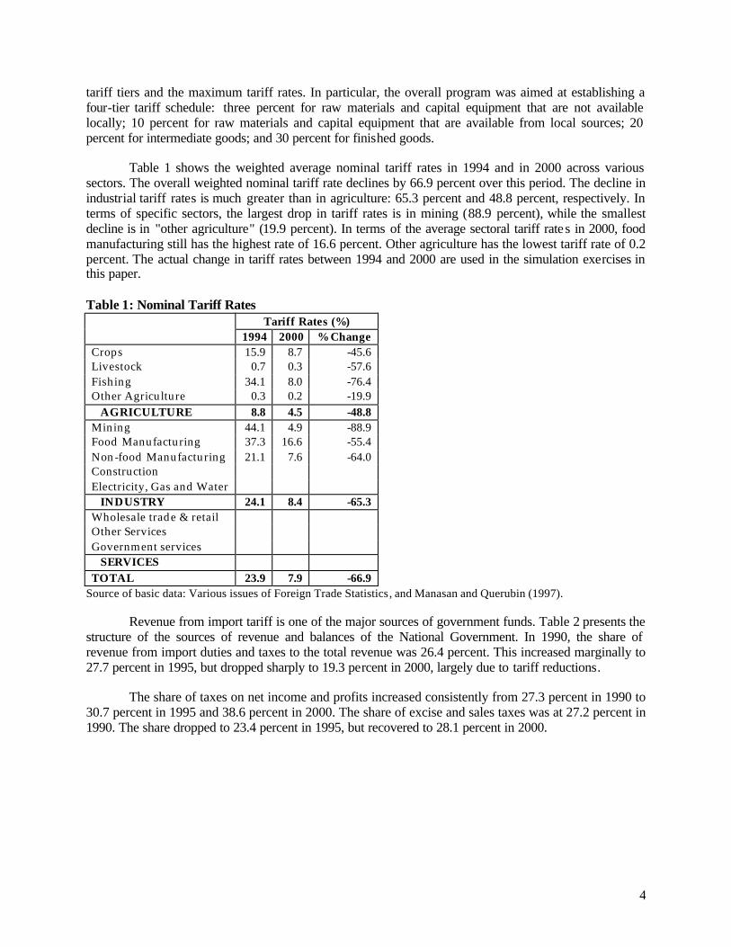
tariff tiers and the maximum tariff rates. In particular, the overall program was aimed at establishing a four-tier tariff schedule: three percent for raw materials and capital equipment that are not available locally; 10 percent for raw materials and capital equipment that are available from local sources; 20 percent for intermediate goods; and 30 percent for finished goods. Table 1 shows the weighted average nominal tariff rates in 1994 and in 2000 across various sectors. The overall weighted nominal tariff rate declines by 66.9 percent over this period. The decline in industrial tariff rates is much greater than in agriculture: 65.3 percent and 48.8 percent, respectively. In terms of specific sectors, the largest drop in tariff rates is in mining (88.9 percent), while the smallest decline is in "other agriculture" (19.9 percent). In terms of the average sectoral tariff rates in 2000, food manufacturing still has the highest rate of 16.6 percent. Other agriculture has the lowest tariff rate of 0.2 percent. The actual change in tariff rates between 1994 and 2000 are used in the simulation exercises in this paper. Table 1: Nominal Tariff Rates Tariff Rates (%) 1994 2000 % Change Crops 15.9 8.7 -45.6 Livestock 0.7 0.3 -57.6 Fishing 34.1 8.0 -76.4 Other Agriculture 0.3 0.2 -19.9

AGRICULTURE 8.8 4.5 -48.8 Mining 44.1 4.9 -88.9 Food Manufacturing 37.3 16.6 -55.4 Non-food Manufacturing 21.1 7.6 -64.0 Construction Electricity, Gas and Water

INDUSTRY 24.1 8.4 -65.3 Wholesale trade & retail Other Services Government services

SERVICES TOTAL 23.9 7.9 -66.9

Source of basic data: Various issues of Foreign Trade Statistics, and Manasan and Querubin (1997). Revenue from import tariff is one of the major sources of government funds. Table 2 presents the

structure of the sources of revenue and balances of the National Government. In 1990, the share of revenue from import duties and taxes to the total revenue was 26.4 percent. This increased marginally to 27.7 percent in 1995, but dropped sharply to 19.3 percent in 2000, largely due to tariff reductions. The share of taxes on net income and profits increased consistently from 27.3 percent in 1990 to 30.7 percent in 1995 and 38.6 percent in 2000. The share of excise and sales taxes was at 27.2 percent in 1990. The share dropped to 23.4 percent in 1995, but recovered to 28.1 percent in 2000.

5

Table 2: Sources of Revenue and Balances of National Government (%) 1990 1995 2000 Tax Revenue 83.9 85.7 89.1 Taxes on net Income and Profits 27.3 30.7 38.6 Excise and Sales Taxes 27.2 23.4 28.1 Import Duties and other Import Taxes 26.4 27.7 19.3 Other Taxes 3.0 3.9 3.1 Non-Tax Revenue 14.8 14.0 10.6 Grants 1.3 0.3 0.3 Total 100.0 100.0 100.0 Total Revenue (P billion) 180.9 362.2 507.1 Total Expenditure (P billion) 218.1 350.1 641.8 (Deficit)/Surplus (P billion) (37.2) 12.1 (134.7) (Deficit)/Surplus (% of GNP) (3.5) 0.6 (3.9) Source: Selected Philippine Economic Indicators (BSP)

4. Poverty Profile

Table 3 presents an overview of the poverty situation in the Philippines in 1994. About 41 percent of the population of 67 million was below the poverty line. Poverty levels vary substantially according to the characteristics of the household head. For example , while 26.6 percent of female-headed households are poor, 42.6 percent of male-headed households are poor. The incidence also varies substantially with the level of education. In case of female -headed households, 35.9 percent of those with low education (zero education up to third grade) are poor, while only 9.1 percent of those with high education (high school graduate and up) are poor. A similar pattern is observed among male-headed households. Table 3: Poverty indices at the base (%, 1994) Female Male

Index All Total Low-ed High-ed Total Low-ed High-ed All Philippines Headcount index 40.6 26.6 35.9 9.1 42.6 54.2 20.4 Poverty gap 13.5 8.4 11.6 2.2 14.2 18.7 5.8 Poverty severity 6.1 3.7 5.2 0.9 6.4 8.6 2.3 National Capital Region (NCR) Headcount index 10.4 5.8 10.7 2.8 11.4 18.9 7.7 Poverty gap 2.0 1.2 2.4 0.4 2.2 3.8 1.4 Poverty severity 0.6 0.4 0.8 0.1 0.7 1.1 0.4 Urban, excluding NCR Headcount index 34.7 23.3 31.5 9.5 35.5 48.8 19.6 Poverty gap 11.4 6.9 9.9 1.9 12.0 17.0 5.4 Poverty severity 5.2 2.9 4.2 0.7 5.5 7.9 2.2 Rural Headcount index 53.1 40.1 44.9 18.9 54.6 60.6 31.6 Poverty gap 18.2 13.4 15.1 5.8 18.7 21.1 9.7 Poverty severity 8.3 6.1 6.9 2.4 8.5 9.7 4.1 Population and number of poor people ('000) population 67,431 poor 27,373

Source: 1994 Family Income and Expenditure Survey; Low-ed=low education; High-ed=high education

6

Geographical variation in poverty is also substantial. For example, while 10.4 percent of households in the NCR are poor, 53.1 percent of rural households are poor, implying that poverty is primarily a rural phenomenon. Urban areas excluding NCR have a poverty incidence of 34.7 percent. Among the household categories included in the table, rural male -headed households with low education have the highest poverty incidence of 60.6 percent, whereas female-headed households with high education in the NCR have the lowest incidence of 2.8 percent. 5. The Model

5.1 Basic Structure

The model is a standard CGE model (see Appendix A). The CGE model used in the analysis was calibrated to the 1994 SAM of the Philippine economy (Cororaton, 2003a). The model has 12 production sectors, four of which are agricultural: Crops; livestock; fishing; and other agriculture. There are five sectors in industry: Mining; food manufacturing; non-food manufacturing; construction; and electricity, gas and water. The service sector is composed of three sectors: Wholesale and retail trade; other services; government services.

Sectoral output is a fixed coefficient (Leontief) combination of value added and intermediate

inputs. The model distinguishes two categories of factor inputs - labor and capital - which generate sectoral value added through a CES production function. The model distinguishes four types of labor: skilled agriculture labor, unskilled agriculture labor, skilled production labor, and unskilled production labor. Agriculture labor is devoted only to the agriculture sector, while production labor can move across all sectors. Skilled production workers include professionals, managers, and other related workers with at least a high school diploma. Sectoral capital is fixed. In both the product and factor markets, prices adjust to clear the markets.

Consumer demand is based on Cobb-Douglas utility functions. An Armington function is assumed to combine local and imported goods into the composite good consumed on the domestic market. Domestic producers allocate their production between exports and local sales according to a CET function.

The whole 1994 FIES, which consists of 24,797 households , is integrated into the model. A brief discussion of the 1994 SAM and the reconciliation with the FIES is given in Appendix B. 5.2 Model Closure

The model closure in the analysis has the following features. First, real government spending is assumed fixed to control for any possible welfare effects of variations in government spending. Nominal total government income is also held fixed. Any reduction in government income from tariff reduction is compensated endogenously either by direct income taxes on households or indirect taxes or both. Nominal (and real) government savings are flexible to absorb changes in the endogenously determined price of total real government consumption.

Total real investment is held fixed in order to abstract from intertemporal welfare effects. The

current account balance is assumed constant to avoid a "free-lunch" welfare effect linked to capital inflows. The nominal exchange rate is the numerary. The foreign trade sector is effectively cleared by changes in the real exchange rate, which is the ratio of the nominal exchange rate multiplied by the world export prices and divided by the local prices. The propensities to save of the various household groups in the model adjust proportionately to accommodate changes in the investment price index and government

7

savings , given the fixed total real investment assumption. This is done through a factor in the household saving function that adjusts endogenously. Changes in household savings are small, as they are solely the result of changes in investment and government consumption prices. 5.3 Income Sources and Consumption Patterns of the Poor and Non-Poor

Trade liberalization influences household poverty through its impacts on household income and consumer prices, which are likely to vary substantially between households. In the tables presented in this section we contrast average values for poor and non-poor households. However, it should be noted that within each of these groups, income sources and consumption patterns vary much more, which motivates our use of CGE microsimulation techniques. Table 4 shows that the sources of income vary substantially between the poor and the non-poor in each of the major regions (all Philippines, NCR, urban excluding NCR, and rural). For example, poor households derive a much larger share of their income from agricultural factors (49.4 percent (=2.9+28.6+17.9)) than do non-poor households (10.4 percent (=1.5+4.3+4.5). In contrast non-poor households are more dependent on production labor income. Note also that the poor derive relatively more income from unskilled labor, whereas the non-poor depend heaving on skilled labor income. The same general pattern is observed when comparing poor and non-poor households in each of the major regions , particularly outside the national capital region. As we could expect, rural households depend much more on agricultural income, with a particularly strong contrast between poor households in rural vs. urban areas. Table 4: Sources of Household Income (% share )

Sources of Household All NCR Urban, no NCR Rural Income Poor N-poor Poor N-poor Poor N-poor Poor N-poor

Agriculture skilled 2.9 1.5 0.4 0.2 2.6 2.2 3.4 2.7 Agriculture unskilled 28.6 4.3 2.3 0.0 22.1 3.5 34.9 13.6 Production skilled 10.9 38.6 45.0 40.7 15.0 42.3 5.2 28.8

Lab

or

Production unskilled 10.4 7.0 20.4 4.6 12.7 8.0 8.1 9.9 Agriculture 17.9 4.5 0.3 0.2 11.7 3.4 23.3 14.3 Industry 10.6 11.3 6.6 9.5 12.4 13.3 9.9 11.3 Service (wholesale & retail) 3.7 5.9 7.6 5.4 4.7 7.1 2.7 4.8

Cap

ital

in:

Service (others) 5.1 10.6 10.2 14.3 7.3 9.7 3.3 5.1 Dividends 0.0 7.7 0.0 18.7 0.0 0.4 0.0 0.1 Transfers 9.1 5.1 5.8 3.5 10.6 6.2 8.5 6.1 Rest of the World 0.8 3.4 1.3 2.9 1.0 3.8 0.7 3.4 100.0 100.0 100.0 100.0 100.0 100.0 100.0 100.0

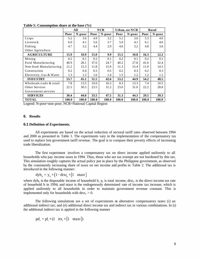
Legend: N-poor=non-poor; NCR=National Capital Region In Table 5, we summarize the consumption patterns of households. The three major items in the consumer basket of households are food manufacturing, other services, and non-food manufacturing. Consumption patterns vary across households. The poor, particularly in rural areas, consume relatively more agricultural and industrial goods, and relatively less services. The share of food manufacturing in the basket of the poor is also much higher than for the non-poor. Among the poor, rural poor households have relatively higher shares of food manufacturing than those in the NCR and other urban areas.

8

Table 5: Consumption share at the base (%) All NCR Urban, no NCR Rural Poor N-poor Poor N-poor Poor N-poor Poor N-poor Crops 5.2 3.6 4.9 3.2 5.1 3.6 5.3 4.0 Livestock 6.0 4.1 5.6 3.7 5.9 4.1 6.1 4.6 Fishing 4.7 3.2 4.4 2.9 4.6 3.2 4.8 3.6 Other Agriculture

AGRICULTURE 15.9 10.9 15.0 9.9 15.5 10.8 16.3 12.2 Mining 0.2 0.1 0.2 0.1 0.2 0.1 0.2 0.1 Food Manufacturing 40.9 28.1 37.6 24.7 40.2 27.8 41.6 32.4 Non-food Manufacturing 11.2 15.3 11.8 15.9 11.3 15.4 11.0 14.5 Construction 0.2 0.4 0.3 0.5 0.2 0.3 0.2 0.3 Electricity, Gas & Water 1.3 1.2 1.6 1.4 1.3 1.2 1.2 1.1

INDUSTRY 53.7 45.1 51.5 42.6 53.2 44.9 54.2 48.5 Wholesale trade & retail 7.8 13.5 10.0 16.3 8.3 13.3 7.4 10.5 Other Services 22.5 30.5 23.5 31.2 23.0 31.0 22.2 28.8 Government services

SERVICES 30.4 44.0 33.5 47.5 31.3 44.3 29.5 39.3 TOTAL 100.0 100.0 100.0 100.0 100.0 100.0 100.0 100.0

Legend: N-poor=non-poor; NCR=National Capital Region 6. Results

6.1 Definition of Experiments.

All experiments are based on the actual reduction of sectoral tariff rates observed between 1994 and 2000 as presented in Table 1. The experiments vary in the implementation of the compensatory tax used to replace lost government tariff revenue. The goal is to compare their poverty effects of increasing trade liberalization.

The first experiment involves a compensatory tax on direct income applied uniformly to all households who pay income taxes in 1994. Thus, those who are tax exempt are not burdened by this tax. This simulation roughly captures the actual policy put in place by the Philippine government, as observed by the consistently increasing share of taxes on net income and profits in Table 2. The additional tax is introduced in the following manner:

[ ]( )h h hdyh y 1 dtxr 1 ntaxr= × − × +

where dyhh is the disposable income of household h, yh is total income, dtxrh is the direct income tax rate of household h in 1994, and ntaxr is the endogenously determined rate of income tax increase, which is applied uniformly to all households in order to maintain government revenue constant. This is implemented only for households with dtxrh > 0.

The following simulations are a set of experiments on alternative compensatory taxes: (i) an additional indirect tax; and (ii) additional direct income tax and indirect tax in various combinations. In (i) the additional indirect tax is applied in the following manner

[ ]i i ipd pl (1 itx ntaxr )= × + × 1+

9

where pdi is the domestic price of sector i, pli is this same price net of indirect taxes, itxi is the sectoral indirect tax rate in 1994, and ntaxr is the endogenously determined rate of increase in indirect tax rates, which is applied uniformly to all sectors to compensate the lost tariff revenue. In (ii) , both income and indirect taxes are adjusted simultaneously in various combinations and in the following manner

(1) [ ]( )h h h dtxrdyh y 1 dtxr 1 ntaxr k= × − × + × and [ ]i i i itxpd pl (1 itx ntaxr k )= × + × 1+ ×

kitx = 1; kdtxr = {0.1, 0.2, 0.3,…, 0.9}

(2) [ ]( )h h h dtxrdyh y 1 dtxr 1 ntaxr k= × − × + × and [ ]i i i itxpd pl (1 itx ntaxr k )= × + × 1+ ×

kdtxr = 1; kitx = {0.1, 0.2, 0.3,…, 0.9} The results of the first experiment will be discussed in detail. We trace the transmission mechanism through which changes in tariff affect income distribution and poverty. The results of the following simulations will be summarized in terms of their effects on household income, consumer prices and poverty. 6.2 Simulation results: Tariff Reduction with Compensatory Direct Income Tax

a) Macro results Before looking in detail at the sectoral, factor and household-level results, Table 6 provides an

overview of the macro effects of the 66.9 percent reduction in the average nominal tariff rate.

Table 6: Macro Effects with Compensatory Direct Income Tax Change (%) Average nominal tariff rate -66.90 Prices:

Import prices in local currency -10.40 Consumer prices -2.87 Local cost of production -2.59

Real exchange rate change 4.10 Import volume 5.27 Export volume 5.41 Domestic production for local sales -0.66 Domestic consumption 0.47 Total output 0.40

Import prices, in local currency (peso) terms, drop by 10.40 percent. This results in a fall in

consumer prices of 2.87 percent, while the local cost of production declines by 2.59 percent. Since the nominal exchange rate and world prices (in foreign currency terms) are fixed, the decline in domestic prices results in a real exchange rate depreciation of 4.1 percent. In reaction, export volume increases by 5.41 percent. The drop in import prices also translates into 5.27 percent higher import volume. The slight decline in domestic production sold on the local market (0.66) percent indicates some crowding out effects on domestic production of higher import volume. However, the net effect on domestic

10

consumption is an increase of 0.47 percent. Despite the crowding out effects on domestic production for local sales, the slightly higher growth in export volume than the import volume results in some improvement in the overall output by 0.4 percent. b) Production and Trade Impacts

The initial impact of trade liberalization is felt in the Philippines foreign trade and production sectors. These subsequently feed into the factor markets, household income and consumer prices, as we will see in the subsequent sections. Table 7 presents the trade and production elasticities and parameters, which represent the initial pre-liberalization situation in 1994. We first note the overwhelming concentration of the Philippines trade in the non-food manufacturing sector. It is clear that this sector will be strongly affected by trade liberalization. In terms of production, both the food and the non-food manufacturing sector have the lowest value-added-output ratio, 30.8 percent and 29.7 percent, respectively. The highest is in other agriculture at 82.3 percent. Although non-food manufacturing has the lowest value added-output ratio, it is the third highest contributor to national value added (13.4 percent) given the large size of this sector. The biggest contributor is other services (26.6 percent of national value added), followed by wholesale trade and retail (14.3 percent). In terms of contribution to the overall output, the non-food manufacturing sector has the highest share of 23 percent, followed by other services. In summary, the non-food manufacturing sector is a dominant sector of the economy, especially in foreign trade. Table 7: Elasticities and Parameters Trade Production * Elasticities** Exports (%)* Imports (%)* VA* X* Capital

Sectors Armington

CET

Share (ei/e)

Intensity (ei/xi)

Share (mi/m)

Intensity (mi/qi) vai/xi*

Share (vai/va)

Share (xi/x)

Labor Ratio*

Crops 1.95 1.27 3.1 7.5 0.7 1.7 77.7 10.3 6.8 0.98 Livestock 1.40 0.40 0.0 0.1 0.6 2.6 58.1 4.5 4.0 0.99 Fishing 1.10 1.50 3.3 20.8 0.0 0.2 71.7 3.7 2.7 1.79 Other Agriculture 0.85 0.40 0.1 2.6 82.3 1.4 0.9 1.00

AGRICULTURE 6.4 7.5 1.5 1.8 71.4 20.0 14.3 Mining 1.10 1.50 2.4 43.1 6.5 66.3 55.0 1.0 0.9 1.15 Food Manufacturing 1.08 1.20 9.0 10.2 5.4 6.3 30.8 8.8 14.7 1.74 Non-food Manufacturing 0.92 1.37 48.0 34.7 76.1 45.3 29.7 13.4 23.0 1.23 Construction 1.20 1.20 0.3 0.8 0.9 2.6 52.8 5.5 5.3 1.28 Electricity, Gas and Water 1.20 1.20 0.2 1.2 53.0 2.8 2.7 2.97

INDUSTRY 59.9 21.3 88.8 28.4 34.5 31.6 46.7 Wholesale trade & retail 1.20 1.20 14.2 20.9 64.1 14.2 11.3 1.95 Other Services 1.20 1.20 19.4 14.6 9.7 7.8 61.4 26.6 22.1 1.64 Government services - - 69.0 7.7 5.7

SERVICES 33.7 14.3 9.7 7.8 63.3 48.5 39.1 TOTAL 100.0 16.6 100.0 17.4 51.0 100.0 100.0 Where ei : exports va: value added mi : imports qi : domestic consumption x : output * Based on the 1994 SAM; ** Based on estimates of Clarete and Warr (1992)

Table 8 presents price and volume effects at the sectoral level. We note that import prices (pm)

fall much more in the industria l sector. It is thus unsurprising that the import (m) response is also greatest for industrial imports. In response, domestic producers experience reduced volume (d) and prices (pl and pd) for local sales. Combined with lower import prices, this leads to a general decline in consumer prices (pq), particularly for industrial goods. Consumers substitute a portion of their consumption (q) from agricultural to the relatively cheaper industrial goods. Local producers react to lower prices on the local

11

market by increasing their exports, once again primarily in the industrial sector and, especially, the non-food manufacturing sector. This is both due to the decline in local prices and the high initial export intensity and share of this sector (Table 7). Consequently, total output (x) of this sector improves by 4.2 percent while others decline or increase only marginally. Clearly, the reallocation effects favor industry as a whole through the effects on the non-food manufacturing sector. Overall agriculture output declines by 1.4 percent, while overall industry improves by 1.4 percent. Service sector production slides marginally by 0.2 percent.

Table 8: Effects on Prices and Volumes (direct income tax) Price Changes (%) Volume Changes (%) pmi pli pdi pqi pxi mi di qi ei xi Crops -5.9 -1.3 -1.3 -1.4 -1.2 8.0 -1.7 -1.5 0.0 -1.5 Livestock -0.4 -1.7 -1.7 -1.7 -1.7 -3.8 -1.9 -2 -1.3 -1.9 Fishing -18.5 -2.1 -2.1 -2.1 -1.6 20.5 -1.5 -1.5 1.7 -0.8 Other Agriculture -0.1 0.2 0.2 0.2 0.2 0.3 0.1 0.1 0.1

AGRICULTURE -3.1 -1.4 -1.4 -1.5 -1.3 2.4 -1.6 -1.5 0.8 -1.4 Mining -25.8 -9.4 -9.4 -21.8 -2.1 10.4 -11.4 4.2 2.7 -5.2 Food Manufacturing -13.9 -2.3 -2.3 -3.3 -4.0 12.8 -1.7 -0.6 1.1 -1.4 Non-food Manufacturing -10.4 -6.2 -6.2 -8.3 -3.4 5.4 1.0 3.2 10.2 4.2 Construction -3.4 -3.4 -3.4 -2.0 -5.4 -1.3 -1.4 2.9 -1.3 Electricity, Gas and Water -2.1 -2.1 -2.1 -0.5 0.3 0.3 2.8 0.3

INDUSTRY -11.7 -4.1 -4.1 -6.5 -3.2 6.1 -0.5 1.5 8.4 1.4 Wholesale trade & retail -0.7 -0.7 -0.7 -0.5 -0.4 -0.4 0.4 -0.3 Other Services -1.3 -1.3 -1.2 -1.1 -2.0 -0.4 -0.5 1.2 -0.1 Government services -0.4 0.0

SERVICES -1.1 -1.1 -1.1 -0.9 -2.0 -0.4 -0.2 0.9 -0.2 TOTAL -10.4 -2.6 -2.6 -4.1 -2.0 5.3 -0.7 0.5 5.4 0.4 Where pqi: composite commodity prices qi: domestic consumption pmi : import (local) prices pxi: output prices ei: exports pli : domestic prices (net of taxes) mi: imports xi: total output pdi: domestic prices (inc. taxes) di: domestic sales

The reallocation effects favoring industry have important consequences in terms of factors

remuneration, as shown in Table 9. Both the volume and price of value added decline for agriculture and increase for industry, particularly for the non-food manufacturing sector. Note that the increase in the non-food manufacturing value added price is largely due to a reduction in its input costs, as most of these inputs come from within this sector where consumer prices fell most. As industry is relatively more capital-intensive, the rate of return to industrial capital increases by 3.0 percent for all industry, due almost entirely to a 10.8 percent increase in the returns to capital in the non-food manufacturing sector. The return to capital in agriculture declines by 1.9 percent as a result of falling prices in this sector. These sectoral price changes also result in a decline in wages for agricultural workers, whereas they improve for production workers. Note that there is also some movement of skilled and unskilled production labor (L3 and L4) towards the non-food manufacturing sector. By assumption, skilled and unskilled agriculture labor (L1 and L2) are employed only in the agriculture sector. The average rate of return to capital and wage improve by 0.9 percent and 1.0 percent, respectively.

12

Table 9: Effects on the Factor Market (direct income tax) Value Added Change (%) in Labor Demand Changes (%) Agricultural Production vai pvai ri, % All Skilled Unskilled Skilled Unskilled Crops -1.5 -0.6 -2.1 -3.0 -0.1 -0.1 -3.3 -4.8 Livestock -1.9 -1.0 -2.9 -3.8 -0.9 -0.9 -4.1 -5.6 Fishing -0.8 -0.6 -1.4 -2.3 0.6 0.6 -2.7 -4.1 Other Agriculture 0.1 1.1 1.2 0.2 3.2 3.2 -0.1 -1.6

AGRICULTURE -1.4 -0.5 -1.9 -2.9 -3.2 -4.7 Mining -5.2 -5.0 -10.0 -10.8 -11.1 -12.5 Food Manufacturing -1.4 -1.5 -2.8 -3.8 -4.1 -5.5 Non-food Manufacturing 4.2 6.3 10.8 9.7 9.3 7.7 Construction -1.3 -0.7 -2.0 -2.9 -3.2 -4.7 Electricity, Gas and Water 0.3 2.0 2.3 1.3 1.0 -0.6

INDUSTRY 1.0 2.1 3.0 2.7 2.2 1.1 Wholesale trade & retail -0.3 0.4 0.2 -0.8 -1.1 -2.6 Other Services -0.1 0.7 0.6 -0.4 -0.7 -2.2 Government services 0.0 1.0 0.0 -0.3 0.0

SERVICES -0.2 0.6 0.4 -0.3 -0.7 -2.2 TOTAL -0.02 0.9 0.9

Change in average wage, % --> 1.0 -1.9 -1.9 1.3 2.9

where vai : value added; pvai : value added prices; ri: rate of return to capital We now explore how these factor price changes affect household income by type of household. We summarize in Table 10 the shares in Table 4 into income from factors employed in the agricultural and non-agricultural sectors. We note that poor rural households rely heavily on income from factors employed in agriculture (61.6 percent of their total income), as compared to the non-poor (30.5 percent). Table 10: Sources of Income by Factors in Agriculture and Non-Agriculture (% share ) Labor & capital Labor & capital income from income from Other

Household Location & Type agriculture /1 non-agriculture /2 Income/3 All Poor 49.4 40.7 9.9 Non-poor 10.4 73.4 16.2 National Capital Region Poor 3.1 89.7 7.2 (NCR) Non-poor 0.4 74.5 25.1 Urban, excluding NCR Poor 36.4 52.0 11.6 Non-poor 9.1 80.5 10.4 Rural Poor 61.6 29.2 9.2 Non-poor 30.5 59.9 9.6 Source: 1994 Family Income and Expenditure Survey /1 sum of skilled labor, unskilled labor and capital in agriculture in Table 4 /2 sum of skilled labor, unskilled labor and capital in industry and service in Table 4 /3 sum of dividends, transfers, and rest of the world in Table 4

As observed earlier, agricultural factor prices decline while non-agriculture factor prices generally improve. The impact on household income is shown in Table 11 where the weighted average change in labor and capital income from agriculture for rural households is –0.8 percent, and for urban households, excluding the NCR, is –0.3 percent. Poor urban households also rely fairly heavily also on agricultural factor income: 36.4 percent of their total income. Thus, on the whole, factor income from agriculture declines by –0.3 percent.

13

As a result of the generally rising factor prices in non-agriculture, income from these factors generally increases. However, rural households have a smaller increase in non-agricultural factor income compared to households in the NCR and other urban areas. The total net factor income effect is 0.9 percent, but varies across households. Households in the NCR enjoy the greatest increase (1.4 percent). Households in urban areas outside the NCR have a 1.1 percent improvement in their total net factor income. Rural households have the least effect of 0.2 percent.

Table 11: Household Labor and Capital Factor Income Effects (weighted % change from base*), direct income tax Labor & capital Labor & capital Total

income from income from Labor & capital Household Location agriculture non-agriculture Income

All -0.3 1.3 0.9 NCR * 0.0 1.4 1.4 Urban, excluding NCR -0.3 1.4 1.1 Rural -0.8 1.0 0.2 * growth multiplied by share to total labor and capital income

The impact of all these on income distribution is presented in Table 12 where the results on the Gini coefficient are shown. The Gini coefficient before and after the tariff change is computed in the following manner:

Gini coefficient = i j i j2 i j

1w w y y

2 n × × − ×

∑ ∑

where n is the overall population, wi is the number people in household i ( ii

w n=∑ ) and yi is household income. The Gini coefficient increases from 0.464 to 0.467, indicating a worsening of income inequality by 0.46 percent. Table 12: Gini Coefficient, direct income tax Before (base) After Gini 0.464 0.467 (% change from base) 0.46% Standard deviation of Gini 0.003 0.003

The effects on poverty are measured by the Foster-Greer-Thorbecke (FGT) indices. In general,

the FGT poverty index is given by3

aqi

ai=1

z - y1P

n z =

∑

where n is population size, q is the number of people below poverty line, yi is income, and z is the poverty line. The poverty line is based on the cost of basic food requirements and an assumed minimal share on non-food consumption. The parameter α can have three possible values, each one indicating a measure of poverty. The headcount index of poverty has α = 0. This is the common index of poverty, which

3See Ravallion (1992) for a detailed discussion.

14

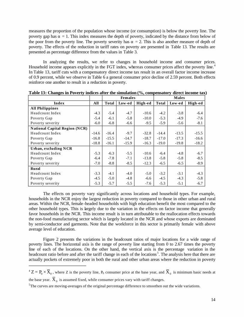
measures the proportion of the population whose income (or consumption) is below the poverty line. The poverty gap has α = 1. This index measures the depth of poverty, indicated by the distance from below of the poor from the poverty line. The poverty severity has α = 2. This is also another measure of depth of poverty. The effects of the reduction in tariff rates on poverty are presented in Table 13. The results are presented as percentage difference from the values in Table 3. In analyzing the results, we refer to changes in household income and consumer prices. Household income appears explicitly in the FGT index, whereas consumer prices affect the poverty line.4 In Table 13, tariff cuts with a compensatory direct income tax result in an overall factor income increase of 0.9 percent, while we observe in Table 6 a general consumer price decline of 2.59 percent. Both effects reinforce one another to result in a reduction in poverty. Table 13: Changes in Poverty indices after the simulation (%, compensatory direct income tax)

Females Males Index All Total Low-ed High-ed Total Low-ed High-ed

All Philippines Headcount Index -4.3 -5.4 -4.7 -10.6 -4.2 -3.8 -6.4 Poverty Gap -5.4 -6.1 -5.8 -10.0 -5.3 -4.9 -7.6 Poverty severity -6.0 -6.8 -6.6 -9.5 -5.9 -5.6 -8.1 National Capital Region (NCR) Headcount Index -14.6 -16.4 -9.7 -32.8 -14.4 -13.5 -15.5 Poverty Gap -16.8 -15.5 -14.7 -18.7 -17.0 -17.3 -16.6 Poverty severity -18.8 -16.1 -15.9 -16.3 -19.0 -19.8 -18.2 Urban, excluding NCR Headcount Index -5.3 -6.3 -5.5 -10.6 -6.4 -4.8 -6.7 Poverty Gap -6.4 -7.8 -7.1 -13.8 -5.8 -5.8 -8.5 Poverty severity -7.0 -8.8 -8.5 -12.3 -6.5 -6.5 -8.9 Rural Headcount Index -3.3 -4.1 -4.0 -5.0 -3.2 -3.1 -4.3 Poverty Gap -4.5 -5.0 -4.8 -6.6 -4.5 -4.3 -5.8 Poverty severity -5.3 -5.7 -5.5 -7.6 -5.3 -5.1 -6.7

The effects on poverty vary significantly across locations and household types. For example, households in the NCR enjoy the largest reduction in poverty compared to those in other urban and rural areas. Within the NCR, female-headed households with high education benefit the most compared to the other household types. This is largely due to the variation in the effects on factor income that generally favor households in the NCR. This income result is in turn attributable to the reallocation effects towards the non-food manufacturing sector which is largely located in the NCR and whose exports are dominated by semi-conductor and garments. Note that the workforce in this sector is primarily female with above average level of education. Figure 2 presents the variations in the headcount ratios of major locations for a wide range of poverty lines. The horizontal axis is the range of poverty line starting from 0 to 2.67 times the poverty line of each of the locations. On the other hand, the vertical axis is the percentage variation in the headcount ratio before and after the tariff change in each of the locations 5. The analysis here that there are actually pockets of extremely poor in both the rural and other urban areas where the reduction in poverty 4

0 0Z P X= × , where Z is the poverty line, P0 consumer price at the base year, and 0X is minimum basic needs at

the base year. 0X is assumed fixed, while consumer prices vary with tariff changes. 5The curves are moving-averages of the original percentage difference to smoothen out the wide variations.

15

as a result of tariff reduction is greater than those households in the NCR. These individuals have incomes ranging from 0.12 per cent to 0.33 per cent of the poverty line (approximately between P1,000 and P3,000 in 1994 prices). Beyond this limited range, the reduction in poverty in the NCR dominates those in both the urban and rural areas. Furthermore, it is also clear from the figure that rural households consistently have the smallest reduction of poverty within the latter range.

Figure 2: Variations in Headcount Ratio Curves, by Major Location

-25.0

-20.0

-15.0

-10.0

-5.0

0.0

Poverty line multiples

% D

iffe

renc

e of

Hea

dcou

t Rat

io,

Bef

ore

and

Aft

er T

arif

f Cha

nge

UrbanNCR

Rural

6.3 Sensitivity Analysis on Compensatory Taxes.

Table 14 presents the results of the sensitivity analysis on various combinations of compensatory taxes. In Panel A the compensatory indirect tax has its full value, while the compensatory direct income tax varies with k, where k ranges from 0 to 1. If k=0.0 the reduction in tariff revenue is compensated only by indirect tax alone. If k=1.0 the compensatory tax is through identical variations in the indirect tax and direct income tax. The variable ntaxr adjusts automatically in the model to clear the reduction in tariff revenue. The value of this variable can also be considered as an indicator of the degree of distortion created by the additional compensatory tax. In Panel A where k = 0.0, the only compensatory tax is the additional indirect tax. The variable ntaxr has the highest value under this scenario because, as we have noted earlier, the additional indirect tax does not only create an additional wedge between the local cost of production and the domestic price, it also changes the relative sectoral domestic price ratios. However, as k is increased to 1, the value of ntaxr diminishes. Take the case of k=0.0. Overall poverty incidence increases by 1 percent. The poverty incidence is also observed to increase in urban areas outside of NCR and in rural areas by 0.94 percent and 1.09 percent, respectively. Two factors drive this result: the reduction in household income and the much smaller reduction in consumer prices. Household incomes decline because factor prices drop; the overall rate of return to capital decreases by 1.19 percent and the average wage rate declines by 1.03 percent. The drop in factor prices is due to a reduction in the value added price of 1.13 percent, which is caused by the additional indirect tax. Furthermore, the much lower reduction in consumer prices (–0.36 percent) is again due to the additional indirect tax that mitigates the full impact of the reduction of tariff rates on domestic prices.

16

Table 14: Sensitivity Analysis on Various Compensatory Tax Combinations (% change from base) compensatory tax on indirect tax multiplied by 1.0

Panel A Base compensatory tax on direct income tax multiplied by k, where k is Values k=0.0 k=0.1 k=0.2 k=0.3 K=0.4 k=0.5 k=0.6 k=0.7 k=0.8 k=0.9 k=1.0 Ntaxr 0 0.828 0.335 0.209 0.152 0.120 0.099 0.084 0.073 0.064 0.058 0.052

All Philippines 40.59 1.00 -1.98 -2.99 -3.35 -3.55 -3.69 -3.79 -3.82 -3.86 -3.89 -3.92 NCR 10.40 -0.29 -8.14 -10.17 -10.91 -11.63 -11.63 -12.32 -12.52 -12.85 -12.85 -12.85 Urban, no NCR 34.70 0.94 -2.66 -3.89 -4.40 -4.55 -4.67 -4.79 -4.81 -4.83 -4.83 -4.83

Po

vert

y

Hea

dcou

nt

Rural 53.12 1.09 -1.33 -2.19 -2.45 -2.65 -2.81 -2.86 -2.89 -2.92 -2.97 -3.01 Household income -0.92 0.09 0.35 0.47 0.54 0.58 0.61 0.64 0.65 0.67 0.68 Avg. VA price -1.13 0.07 0.38 0.52 0.60 0.66 0.69 0.72 0.74 0.76 0.77 Avg. capital return -1.19 0.05 0.36 0.50 0.58 0.64 0.67 0.70 0.72 0.74 0.75 Avg. wage rate -1.03 0.16 0.46 0.60 0.67 0.72 0.76 0.79 0.81 0.82 0.84 Consumer price -0.36 -1.86 -2.24 -2.41 -2.51 -2.57 -2.62 -2.65 -2.68 -2.70 -2.71 compensatory tax on direct income tax multiplied by 1.0

Panel B Base compensatory tax on indirect tax multiplied by k, where k is Values k=0.0 k=0.1 k=0.2 k=0.3 K=0.4 k=0.5 k=0.6 k=0.7 k=0.8 k=0.9 ntaxr 0 0.053 0.055 0.055 0.055 0.054 0.054 0.054 0.053 0.053 0.053

All Philippines 40.59 -4.38 -4.28 -4.24 -4.19 -4.17 -4.09 -4.07 -4.06 -4.01 -3.96 NCR 10.40 -14.65 -13.98 -13.98 -13.63 -13.63 -13.44 -13.44 -13.44 -13.08 -12.85 Urban, no NCR 34.70 -5.30 -5.30 -5.23 -5.19 -5.14 -5.04 -4.99 -4.96 -4.91 -4.88

Po

vert

y

Hea

dcou

nt

Rural 53.12 -3.40 -3.29 -3.25 -3.21 -3.20 -3.14 -3.14 -3.13 -3.10 -3.05 Household income 0.78 0.78 0.77 0.75 0.74 0.73 0.72 0.71 0.70 0.69 Avg. VA price 0.89 0.88 0.87 0.86 0.84 0.83 0.82 0.81 0.79 0.78 Avg. capital return 0.87 0.87 0.86 0.84 0.83 0.82 0.80 0.79 0.78 0.77 Avg. wage rate 0.96 0.95 0.94 0.92 0.91 0.90 0.88 0.87 0.86 0.85 Consumer price -2.89 -2.85 -2.84 -2.82 -2.81 -2.79 -2.77 -2.76 -2.74 -2.73 If k is increased to 0.1, the reliance on the compensatory indirect tax is reduced. In this case, the compensatory direct income tax starts generating revenue to partly offset the decline in tariff revenue. Here the degree of distortion created by compensatory indirect tax is reduced as indicated by a lower value of ntaxr (0.335, rather than 0.828). Direct taxes are effectively less distortionary than indirect taxes. The reduction in consumer prices is a lot higher (–1.86 percent) because the impact of the reduction of tariff rates on domestic prices is much larger. Furthermore, because of the relatively lower distortion, the change in the value added price flips to a positive value, which in turn improves factor prices. The positive effect on factor income and the much larger decline in consumer prices reinforce one another to result in a reduction in the poverty incidence. As k is increased to a higher value, the impact on poverty improves. In Panel B the compensatory direct income tax has its full value, while the compensatory indirect tax varies with k, where k ranges from 0 to 0.9. If k=0 compensatory direct income tax is the only tax adjustment that offsets the tariff revenue loss. This has been discussed in detail above. Although ntaxr increases marginally from 0.053 to 0.055 as k is increased to 0.4, in higher values it does not give a very clear indication of the degree of distortion introduced by the compensatory indirect tax because it starts to yie ld, though very slightly, declining values. However, the results on the change in the value added price and the change in the consumer prices clearly show the degree of distortion as k is increased to higher values. The increase in the former decelerates, while the reduction in the latter decreases. As a result, the reduction in poverty indices declines. Actual data in Table 2 show that it is indeed a combination of increasing shares of taxes on net income and profits and excise and sales taxes that offset the decline in the share of import duties and other import taxes. The results of the sensitivity analysis clearly show that in all cases where both compensatory taxes are introduced, poverty incidence declines. However, the decline is a lot higher in the NCR than in other areas.

17

7. Conclusion

The main result of the simulation exercise indicates that the reduction in tariff rates between 1994 and 2000 is generally poverty-reducing. However, the decline is much higher in the NCR than in other areas, especially rural. NCR has the lowest initial poverty incidence while rural has the highest.

This distributive impact results largely from the reallocation effects of tariff reduction that favor the non-food manufacturing sector. Tariff cuts lower the cost of local production and bring about real exchange rate depreciation. Since the non-food manufacturing sector dominates exports in terms of export share and export intensity, the general equilibrium effects of tariff reduction attract resources toward it, resulting in higher factor prices in the sector. Agriculture contracts, while agriculture factor prices decline. Overall income inequality worsens as a result.

The other crucial poverty-reducing effect of tariff reduction is through the lowering of consumer

prices. In fact, the overall reduction in consumer prices is significantly higher than the total increase in household income.

18

References

Bourguignon, F., M. Fournier and M. Gurgand (2000), "Fast Development with a Stable Income Distribution: Taiwan, 1979-1994", Working paper 2000-07, DELTA, Paris.

Clarete, R. and Warr, P. (1992), “The Theoretical Structure of the APEX Model of the Philippine Economy”, (Unpublished manuscript).

Cockburn, J., (2001). “Trade Liberalisation and Poverty in Nepal: A Computable General Equilibrium Micro Simulation Analysis”, Discussion paper 01-18, Centre de Recherche en Économie et Finance Appliquées (Universite Laval), October 2001.

Cogneau, D. (1999), "Labour Market, Income Distribution and Poverty in Antananarivo: A General Equilibrium Simulation", mimeo, DIAL, Paris.

Cogneau, D. and A.S. Robillard (2000), "Growth Distribution and Poverty in Madagascar: Learning from a Microsimulation Model in a General Equilibrium Framework", mimeo, DIAL, Paris.

Cororaton, C., (2003a), “Analyzing the Impact of Trade Reforms on Welfare and Income Distribution Using CGE Framework: The Case of the Philippines” PIDS Discussion Paper Series No. 2003-01.

Cororaton, C. (2003b), “Construction of Philippine SAM for the Use of CGE-Microsimulation Analysis”, (Unpublished manuscript).

Decaluwé, B., J.-C. Dumont and L. Savard (1999), "Measuring Poverty and Inequality in a Computable General Equilibrium Model", Working paper 99-20, CREFA, Université Laval.

Decaluwé, B., A. Patry, L. Savard et E. Thorbecke (2000), "Poverty Analysis within a General Equilibrium Framework", Working paper 9909, Department of Economics, Laval University

De Janvry, A., E. Sadoulet and A. Fargeix (1991), "Politically Feasible and Equitable Adjustment: Some Alternatives for Ecuador", World Development, 19(11): 1577-1594.

Manasan, R. and Querubin, R. (1997), “Assessment of Tariff Reform in the 1990s”, Philippine Institute for Development Studies Discussion Paper No. 97-10.

Orcutt, G. (1957), "A New Type of Socio-Economic System", Review of Economics and Statistics, 58: 773-797.

Orcutt, G. M. Greenberg, J. Korbel and A. Rivlin (1961), Microanalysis of Socioeconomic Systems: A Simulation Study, Urban Institute Press, Washington.

Piggott, J. and J. Whalley (1985), UK Tax Policy and Applied General Equilibrium Analysis, Cambridge, Cambridge University Press.

Ravallion, M. (1994), Poverty Comparisons , Harwood Academic Publisher, New York. Tongeren, F.W. van (1994), "Microsimulation Versus Applied General Equilibrium Models", mimeo,

presented at 5th International Conference on CGE Modeling, October 27-29, University of Waterloo, Canada.

1994 Input-Output Table. National Statistical Coordination Board. 1994 Family Income and Expenditure Survey. National Statistics Office 1994 National Income Accounts. National Statistical Coordination Board. 1994 Annual Survey of Establishments. National Statistics Office 1994 Labor Force Survey. National Statistics Office Philippine Economic Indicators, various issues. Bangko Sentral ng Pilipinas

19

Appendix A: A note on the construction of 1994 SAM and reconciliation with 1994 FIES The construction of the SAM uses data from 19946. The sources of data include the 1994 Input-Output (IO) Table; the 1994 Labor Force Survey (LFS); the various 1994 Annual Survey of Establishments (ASE); the 1994 FIES; 1994 National Income Accounts (NIA); 1994 Government Accounts (GA); and the tariff study of Manasan and Querubin (1997) which covers the period 1990-2000. For the construction of the SAM, two major adjustments are made in the 1994 IO: on the sectoral compensation of employees and the sectoral indirect taxes. The sectoral compensation of employees in the IO is grossly understated because it covers labor payment in the formal sector only. To adjust for this understatement, we do the following:

(i) Derive an overall adjustment factor using the data on household and unincorporated operating surplus and the compensation of employees from the 1994 NIA

NIAT NIA

NIA

Ladj = HH_OS

GDP

×

where adjT is the overall adjustment, HH_OSNIA household and unincorporated operating surplus, LNIA is compensation of employees, GDPNIA.

(ii) Disaggregate the total adjustment factor into sectoral adjustment, adj_i, using the sectoral share of compensation of employees from the IO

IO_ii T

IO

Ladj adj

L

= ×

where LIO_i is the sectoral and LIO the overall total compensation of employees in the IO. The sectoral adji is applied to the original sectoral compensation of employees of the IO to get the adjusted sectoral payment to labor. The sectoral payment to capital is derived residually from the value added, net of indirect taxes, of the IO.

The overall indirect tax from the IO, which is composed of local sales tax and tariff, is also grossly understated compared to the data in the 1994 GA. The adjustments are applied to separately compute for the sectoral tariff revenue and the local indirect tax revenue. The sectoral tariff revenue is computed into two steps. The first step is

ii

i

mm_net

(1 tm )=

+

where m_net_ i is imports of sector i net of tariff, m_i is imports inclusive of tariff, which is the value of sectoral imports taken directly from the IO, and tm_ i is the weighted average nominal tariff rate computed by Manasan and Querubin (1997). The next step is

i i itmrev m_net tm= ×

6A detailed discussion is in Cororaton (2003b).

20

where tmrevi is sectoral tariff revenue. The overall sum of sectoral tmrevi is normalized to the overall tariff revenue in the GA.

The total indirect tax revenue from local sales from the GA is distributed sectorally using the original IO sectoral indirect taxes as share the distribution. This, together with the tmrevi above, replaces the sectoral indirect taxes in the IO. The SAM is balanced through an adjustment process that uses a least square method wherein the squared distance between the cells of the balanced SAM and the original unbalanced SAM is minimized subject to the equality of columns and row totals.

The first major step in the integration of the SAM and FIES is the reconciliation of the expenditure items in the la tter with the sectors in the former. There is no official conversion matrix available in 1994, but there is one in 1990 that we use in our adjustment.

The second major step is the reconciliation of the generation of factor incomes in the SAM and

the sources of income in the FIES. A number of steps are involved to complete the process: 1. Group the households in the FIES according to the level of education of head of family, in

particular the group of zero education to third year high school and the other group of high-school graduates and up. The overall sum of labor income from agriculture in the FIES for the first group is adjusted to the total labor income for unskilled agriculture labor in the SAM. Similarly, the overall sum of labor income from agriculture in the FIES for the second group is adjusted to the total labor income for skilled agriculture labor in the SAM. Income of household from these sources is derived through normalization using the adjusted totals. The same process is applied to labor income from non-agriculture.

2. The sectoral breakdown of entrepreneurial income in the FIES is generally consistent with the

sectoral breakdown in the SAM. Using the assumption that entrepreneurial income is factor income from capital, we reconcile the two by normalizing the former with the latter.

3. Household savings are derived residually.

21

Appendix B: Model Specification No. Equation Eqs.

1 i i ix =va ×kt_in 12

2

-1

rh_vatdtd td-rh_va -rh_va

td td td td td tdva =kt_va × sh_va ×k +(1-sh_va )×l 11

3 ntd ntdva =l 1

4 i i iinp =kt_inp×x 12

5

td

td

1

1+rh_vatd td

td td rh_va

td

pva ×(1-sh_va )l =va ×

w×kt_va

11

6 ntd ntd td,ntd tdtd

ntd

px ×x - mat ×pdl =

w∑

1

7 i i i

wl(j) = ×sh_l(j) ×l

w(j)

48

8 rh_e td_1etd_1e td_1e

1rh_e rh_e

td_1e td_1e td_1e td_1e td_1e td_1ex =kt_x × sh_x ×e +(1-sh_x )×d 10

9 td_0e td_0ex =d 1

10

td_1esig_e

td_1e td_1etd_1e td_1e

td_1e td_1e

pe 1-sh_xe =d × ×

pl sh_x

10

11 rh_m td_1mtd_1m td_1m

1rh_m rh_m

td_1m td_1m td_1m td_1m td_1m td_1mq =kt_q × sh_q ×m +(1-sh_q )×d 9

12 td_0m td_0mq =d 2

13

td_1msig_m

td_1m td_1mtd_1m td_1m

td_1m td_1m

pd sh_qm =d × ×

pm 1-sh_q

9

14 h h hct =dyh -savh 24,797

15 td,h h

td,h

td

kt_ch ×ctch =

pq 272,76

7

16 "s12" "s12"g=px ×x

17 td

td

td

kt_inv ×tinv_nnv =

pqi

11

18 iiy(j)= w(j)×l(j)∑ 4

19 ag agagyk_ag= r ×k∑ 1

20 yk_ind= r ×kind ind ind∑ 1

21 "s10" "s10"yk_ser_tra=r ×k

22

22 "s11" "s11"yk_ser_oth=r ×k

23

h h h hj

h h

h h h

yh = (j)×endw_l(j) +k_yk_ag ×lmda_ag×yk_ag+k_yk_ind ×lmda_ind×yk_ind

+k_yk_ser_tra ×lmda_ser_tra×yk_ser_tra+k_yk_ser_oth ×lmda_ser_oth×yk_ser_oth

+kt_div ×div+trgov ×pindex+yfor

∑

24,797

24 h h hdyh =yh ×(1-dtxrh -ntaxr) 24,797

25

yf=[(1-lmda_ag-lmda_ag_f)×yk_ag+(1-lmda_ind-lmda_ind_f)×yk_ind

+(1-lmda_ser_tra-lmda_ser_tra)×yk_ser_tra+(1-lmda_ser_oth-lmda_ser_oth)×yk_ser_oth]×(1-dtxrf) 1

26 yg=tmrev+dtxrev+itxrev+grant_for 1

27 td_1m td_1mtd_1mtmrev= tm ×m∑ 1

28

h hhdtxrev= (dtxrh +ntaxr)×yh +[(1-lmda_ag-lmda_ag_f)×yk_ag

+(1-lmda_ind-lmda_ind_f)×yk_ind+(1-lmda_ser_tra-lmda_ser_tra)×yk_ser_tra

+(1-lmda_ser_oth-lmda_ser_oth)×yk_ser_oth]×dtxrf

∑

1

29 td td td td_1m td_1m td_1m td_1mtd td_1mitxrev= itxr ×d ×pl + itxr ×m ×pwm ×er×(1+tm )∑ ∑ 1

30 td td,iiin_td = mat∑ 11

31 tinv_n=pinv×tinv_r 1

32 h h hsavh =adj×aps ×dyh 24,797

33 hhsavg=yg-g- trgov ×pindex-paygv_for∑ 1

34 td tdtdpindex= sh_q1 ×pq∑ 1

35

tdkt_inv

td

td

td

pqpinv=

kt_inv

∏ 1

36 td_1m td_1m td_1m td_1mpm =pwm ×er×(1+tm )×(1+itxr ) 9

37 td_1e td_1epe =pwe ×er 10

38

td_1m td_1m td_1m td_1m

td_1m

td_1m

pd ×d +pm ×mpq =

q

9

39 td_0m td_0mpq =pd 2

40

td_1e td_1e td_1e td_1e

td_1e

td_1e

pl ×d +pe ×epx =

x

10

41 td_0e td_0epx =pl 1

42 td td tdpd =pl ×[1+itxr ] 11

43 i i td,i tdtd

i

i

p x × x - mat ×pqpva =

va

∑ 12

44 td td td

td

td

pva ×va -w×lr =

k

11

45 td_0s11 td_0s11,h td_0s11 td_0s11hq = ch +inv +in_td∑ 10

23

46 hhtinv_n= savh +savf+savg+cab∑ 1

47

td_1m td_1mtd_1m

td_1e td_1e htd_1e h

cab=[ pwm ×m +lmda_ag_f×yk_ag+lmda_ind_f×yk_ind+lmda_ser_tra_f×yk_ser_tra

+lmda_ser_oth×yk_ser_oth+div_for+paygv_for- pwe ×e - yfor -grant_for]×er

∑∑ ∑

1

48 iils= l∑ 1

49 iils(j)= l(j)∑ 4

50 "s11" "s11",h "s11" "s11"hleon=q - ch +inv +in_td∑ 1

Total number of equations: 372,358

24

a) Endogenous

b) Variables

Description

No. xi output of sector i 11 vai value added of sector i 12 intpi intermediate input of sector I 12 mattd,i interindustry matrix, sector td and I 132 li aggregate labor demand of sector i 12 l(j)i type j labor in sector i (where j = labor type 1, 2, 3, 4) 48 etd_1e exports of sector td_1e 10 qtd composite demand in sector td 11 mtd_1m imports of sector td_1m 9 cth total consumption of household h 24,797 chtd,h household h consumption in sector td 272,767 invtd investment demand in sector td 11 yl(j) type j labor income 4 yk_ag capital income in agriculture 1 yk_ind capital income in industry 1 yk_ser_tra capital income in service trade 1 yk_ser_oth capital income in service others 1 yhh income of household h 24,797 dyhh disposable income of household h 24,797 yf income of firms 1 tmrev tariff revenue of government 1 itxrev indirect income tax revenue of government 1 dtxrev direct income tax revenue of government 1 intdtd intermediate demand for td 11 tinv_n total investment 1 savhh savings of household h 24,797 savf savings of firms 1 savg savings of government 1 pindex general price 1 pinv price of investment 1 pmtd_1m domestic price of imports of td_1m 9 petd_1e domestic price of exports of td_1e 10 pqtd composite price of td 11 pxi price of output of i 12 pdtd domestic price of td including tax 11 pvai price of value added of i 12 rtd price of capital in td 11 w average wage rate 1 ntaxr compensatory tax 1 pltd local price of td excluding tax 11 dtd domestic demand for td 11 adj adjustment factor in household savings 1 w(j) wage rate of type j labor 4 leon “walras law” variable 1 c) Total number of variables 372,358

25

d) Exogenous e) Variables

Description

No.

yg income of government 1 g total government consumption 1 cab current account balance 1 X”s12” Output of sector 12 (government services) 1 pwetd_1e world price of exports of td_1e 11 pwmtd_1m world price of imports of td_1m 9 er exchange rate 1 ktd capital in td 11 ls total supply of labor 1 ls(j) total supply of type j labor 4 endw_l(j)h household h labor endowment of type (j) labor 99,188 div_for dividends paid to foreigners 1 grant_for foreign grant to government 1 paygv_for debt service payment of government 1 yforh foreign income of household h 24,797 div dividends 1 trgovh government transfer in real terms to household h 24,797 dtxrf direct income tax rate on firms 1 dtxrhh direct income tax rate on household h 24,797 itxrtd indirect tax rate on td 11 tmtd_1m tariff rate on td_1m 9