trade, quality upgrading, and input linkages: theory and ... · trade, quality upgrading, and input...
TRANSCRIPT

Trade, Quality Upgrading, and Input Linkages:Theory and Evidence from Colombia∗
Ana Cecılia Fieler,†Marcela Eslava‡, and Daniel Yi Xu§
July 2017
Abstract
A quantitative model brings together theories linking international trade to quality,technology and demand for skills. Standard effects of trade on importers and exportersare magnified through domestic input linkages. We estimate the model with data fromColombian manufacturing firms before the 1991 trade liberalization. A counterfactualtrade liberalization is broadly consistent with post-liberalization data. It increases skillintensity from 11% to 16%, while decreasing sales. Imported inputs, estimated to beof higher quality, and domestic input linkages are quantitatively important. Economiesof scale, export expansion, and reallocation of production are quantitatively small andcannot explain post-liberalization data.
Keywords: trade liberalization, skill, quality, intermediate inputs, amplification effect.
∗We are very grateful to our editor, Penny Goldberg, and to four anonymous referees whose com-ments have significantly improved earlier drafts. We thank Joaquim Blaum, Hal Cole, Arnaud Costinot,Jonathan Eaton, Juan Carlos Hallak, Oleg Itskhoki, Steve Redding, Ina Simonovska, and Jon Vogel fortheir comments. We are grateful to DANE for making their data available to us and to our researchassistants Pamela Medina, Anderson Ospino, Alvaro Pinzon, Juan Pablo Uribe, and Angela Zorro.†Department of Economics at the University of Pennsylvania and NBER. Corresponding author:
[email protected]‡Department of Economics at Universidad de Los Andes and CEDE. [email protected]§Department of Economics at Duke University and NBER. [email protected]
1 Introduction
After decades of import-substitution policies, numerous developing countries unilaterally
liberalized to international trade in the 1980s and 1990s. These episodes were followed
by broad transformations in manufacturing: Investment, skill intensity, the quality of
inputs and outputs all increased, at the same time that the skill premium rose sharply,
typically by 10% to 20%. Firm size decreased or remained unchanged.1 While many
theories have been developed to explain these findings, their quantitative effect is mostly
unknown, especially of theories involving quality or technology upgrading. To fill this
gap, we develop a unified model and quantify many salient theories using data from a
Colombian manufacturing survey around the 1991 trade liberalization. A unified approach
is warranted because our quantitative analysis shows that direct effects of trade interact
and are magnified through domestic input linkages.
Specifically, the data suggest that decisions on scale, quality, importing and exporting,
and demand for skilled workers are interconnected within and across firms. The connection
within firms is suggested by the correlation between various firm characteristics: Large
firms are skill intensive, participate more in international trade, and have higher price-
adjusted sales (quality or market “appeal”). The connection across firms is suggested by
evidence that high-quality, skill-intensive firms use higher-quality inputs. Since importers
and exporters account for more than 70% of domestic sales and purchases of inputs, their
actions significantly influence the domestic input market.
To incorporate all these interconnections in a quantitative model, we propose a novel,
1Measured productivity typically went up also—see Pavcnik (2002), Khandelwal and Topalova (2011),Trefler (2004), Aw, Roberts, Xu (2011), Eslava et al. (2013) and references there surveyed. Goldbergand Pavcnik (2004, 2007) survey changes in labor market, and Tybout (2008) surveys changes in firmsize. See Verhoogen (2008), Kugler and Verhoogen (2012) and Tovar (2012) for quality improvements,and Holmes and Schmitz (2010) and Das et al. (2013) for case studies. Changes are well-documentedfor middle-income countries, and they are less clear for low-income countries. The main trade partnersof these middle-income countries were at the time high-income countries—not yet China. For Colombia,Eslava et al. (2013) find that a fall in tariffs from 60% to 20% is associated with an increase in theprobability of exiting of about 0.4% points; a within-plant increase in productivity of about 3 log points;and an increase in the correlation between productivity and market share from 0.43 to 0.52.
2

flexible production function. The model features heterogeneous firms that choose their
output quality from a continuum. Higher quality increases the fixed cost of production
and revenue. More productive firms self-select into higher quality since the revenue gain
is proportional to productivity. Quality also changes the firm’s unit cost, its valuation
of skilled labor and quality-differentiated materials. All firms produce goods for final
consumption and input usage so that firms’ quality choices are linked through general
equilibrium prices and demand for inputs. Firms live in a small open economy, and we
allow the relative demand and supply of higher-quality goods to be different abroad. In
sum, quality in the model is a latent variable that links various observable outcomes. The
model imposes a positive correlation between quality and sales, but not its relation to
skill intensity, price, quality of inputs, or import and export participation.
We estimate the model using data from 1982-1988, before the trade liberalization. We
match moments on the joint distribution of firms’ revenue, wages, skill intensity, import
and export statuses and intensities, prices of inputs and output. Given the positive
correlation between these characteristics, parameter estimates imply that the production
of higher quality is intensive in skilled labor and in high-quality inputs, and that the
relative demand and supply of high-quality goods is higher abroad.
With these parameter estimates, the model brings together salient theories on the
effects of international trade on demand for skilled labor. There is selection of higher-
quality, skill-intensive goods into importing and exporting. There are economies of scale
in the production of these goods. Trade leads exporters to upgrade because foreign has
a higher demand for higher-quality goods, and it leads importers to upgrade because
foreign inputs makes it cheaper to produce higher-quality—as in models of offshoring
and of non-homothetic preferences.2 In addition, these previously-proposed direct effects
2Selection appears in Melitz (2003). See Yeaple (2005), Lileeva and Trefler (2010), Bustos (2011),Helpman et al. (2010, 2016) for the economies-of-scale hypothesis. The demand for skill intensive goodsis higher abroad in models of quality-differentiation, e.g. Verhoogen (2008) and Faber (2014), and ofoffshoring, e.g., Feenstra and Hanson (1997), Antras, Garicano and Rossi-Hansberg (2006), Feenstra(2010). For intermediate goods, see Goldberg et al. (2009, 2010, 2016), Kugler and Verhoogen (2012),Burstein, Cravino, Vogel (2013). Ours is not the only mechanism where trade has a positive effect on
3

are amplified in the domestic input market. Because the production of higher quality
is intensive in high-quality inputs, upgrading among importers and exporters increases
the domestic supply and demand for high-quality inputs. The increased supply decreases
the cost of producing higher quality and the increased demand increases profits from
upgrading. Both of these changes give incentives for all firms to upgrade.
To evaluate the role of these various effects in explaining overtime changes in the data,
we simulate a counterfactual trade liberalization in the lines of Colombia in the early
1990s. Like in other unilateral trade liberalizations, imports grew faster than exports in
the medium run, and we allow the trade deficit to increase on par with data. In the
counterfactual, half of firms upgrade quality. Aggregate skill intensity increases from 12%
to 16%, and sales decrease by 7% due to import competition.3 Quality upgrading is greater
among ex ante higher-quality firms, increasing the dispersion in the distributions of skill
intensity and sales. Profits decrease, in line with the opposition of industry associations
to unilateral trade liberalizations in Colombia and elsewhere.
Quantitatively, the model is not far from post-liberalization data though it underesti-
mates the rise in demand for skills (section 6). The main mechanisms increasing quality
and demand for skills in the counterfactual are the decrease in the price of high-quality
foreign inputs and the ensuing increase in the quality of domestic inputs. These changes
both decrease the relative cost of producing higher quality. The novel magnification ef-
fect of domestic inputs is key to generate widespread increases in skill intensity in the
counterfactual—for example, skill intensity increases in 28% of firms that never import
or export. It also matters for aggregate changes in skill intensity because it affects large
firms, which demand most of their inputs domestically in the data and model.
The model’s reconciliation of large and widespread increases in manufacturing skill
intensity with decreases in sales is in line with data and illustrates well the importance
the quality of domestically-oriented firms. For example, in models of perfect competition and constantreturns to scale, the boundary of the firm is not defined and the behavior of exporters and non-exportersis indistinguishable.
3Aggregate skill intensity is interpreted as the share of manufacturing workers with college degrees.
4

of using micro-level data in a quantification exercise. In estimating the model, we allow
firms to differ in their comparative advantage in producing higher quality, and the weak
correlation between sales and wages in the data imply that scale is not a key determinant
of quality in the estimated model.
Special cases of the model allow us to isolate some mechanisms, and repeating the
counterfactual trade liberalization with these special cases yields negligible changes on firm
quality and skill intensity. If the valuation of inputs does not depend on the purchasing
firm’s quality, then the only potential mechanisms are export expansion and returns to
scale. In this case, quality upgrading for non-exporting firms reduces to an investment in
productivity, which is only profitable if sales increase. Since 90% of firms do not export in
the data, this special case cannot explain the widespread increases in skill intensity and
decreases in sales in the data.
Reallocation is isolated in a special case where quality is exogenous. In this case,
demand for skills increases only through reallocation of production across firms, not
within-firms. Since large, skill-intensive firms account for the majority of employment
pre-liberalization, reallocating workers toward them cannot explain the observed increase
in aggregate manufacturing skill intensity. We also provide reduced-form evidence of
within-firm changes in a panel of pre-liberalization data. A decrease in firm-specific input
tariffs is associated with an increase in skill intensity, input and output prices, price-
adjusted sales (measured quality) and export participation and intensity. These results
are consistent with the model where a decrease in input tariffs leads to all these within-firm
changes through quality upgrading.
Relative to the literature on endogenous quality or technology and trade, the model
adds the magnification effect of inputs, and it extends previous models to a quantitative
setting.4 Relative to quantitative work on trade liberalizations, we use data on a much
4See references above. Inputs have a magnification effect in Markusen and Venables (1999) and Jones(2011), but their mechanism relies on the size of the market increasing. Carluccio and Fally (2013)formalize the magnification mechanism in a stylized model of foreign direct investment. The general ideaalso appears in empirical papers such as Javorkic (2004) and Kee and Tang (2016).
5

richer set of firm characteristics to more directly identify the effects of trade on firms,
and we are the first to compare counterfactuals to data, improving our understanding
of the quantitative effects of existing theories. Helpman et al. (2016) and Dix-Carneiro
(2014) use micro-data but observe very few firm characteristics, while others use aggregate
country-sector data.5 The magnification effect of inputs adds complexity to the model,
imposing limits on our analysis. We do not address imperfect labor markets in Helpman et
al. (2016), or differences across sectors in Parro (2013), Burstein, Cravino, Vogel (2013),
Dix-Carneiro (2014), and Lee (2016).
Quality upgrading in the model is a skill biased-technical change. Input linkages high-
lighted here matter for improvements in management, investments in modern equipment,
information technologies, and product design: All these investments are more valuable if
other firms in the production chain incur them.6 Section 2 describes Colombian reforms
and data. The model is in section 3, and the estimation procedure is in section 4. We
present estimation results in section 5 and counterfactuals in section 6. Extensions and
robustness are in section 7. Section 8 concludes.
2 Data and Context
Following international trends, Colombia reduced trade barriers in a broad set of industries
between 1985 and 1991 after decades of import-substitution policies. Non-tariff barriers,
which affected 99.6% of industries in 1984, were removed, and the average manufacturing
tariff fell from 32% to 12%. In 1991, reductions in trade barriers were particularly big,
largely unexpected and isolated from other reforms. The newly-elected Gaviria adminis-
5Helpman et al. and Dix-Carneiro use micro-data from the Brazilian unilateral liberalization. Helpmanet al do not observe sales and use export status to estimate economies of scale. Since export status maybe a good indicator of the ability to compete with foreign firms abroad and at home, it is not clearwhether exporters stand out during the liberalization because of the domestic or foreign market. Parro(2013), Burstein, Cravino, Vogel (2013), Burstein, Vogel (2016), and Lee (2016) use aggregate data.
6Acemoglu and Autor (2010) survey skill-biased technical change, and Voigtlander (2014) providesevidence from the USA that skill-intensive firms source more inputs from other skill-intensive firms. Theinterconnection between firm outcomes is also highlighted in Bloom et al. (2016)
6

tration had designed a four-year plan to reduce trade barriers, but it abruptly implemented
the whole plan after a few months under the impression that uncertainty was holding
back changes in firms. Faced with a surge in import competition, industry associations
mounted a strong opposition that ultimately led congress to block other market-oriented
reforms.7 Exports grew slowly initially and picked up only after a large devaluation of
Colombian pesos in 1999—after the period covered by most studies documenting changes
in Colombian manufacturing and labor markets.8
The Colombian Annual Manufacturing Survey covers all manufacturing plants with
10 or more workers. A plant is interpreted as a firm in the model.9 The estimation uses
data from 1982 through 1988. For each plant and year, these data contain the value of
domestic and export sales, and spending on domestic and imported materials. The survey
is uniquely rich in recording quantities and values of all goods produced and all materials
used by 8-digit product categories.10
The number of workers and wage bill are reported separately for managers, technicians
and production workers. We take managers and technicians to be white-collar workers,
but allow measurement error to distinguish them from skilled workers in the model. This
classification is not as detailed as occupational data, but it is superior to the usual split
into production and non-production workers where skilled technicians are usually classified
as production. Using these white-collar shares, appendix A.1 replicates the results in
Attanasio, Goldberg, Pavcnik (2004, AGP henceforth) who use a Colombian household
survey and observe college graduation rates.
For post-liberalization data, 1994 is the last year for which we have a consistent mea-
sure of skills—the classification of employees changed afterward. In 1991, data on imports
7Edwards (2001) describes the political economy of reforms in Colombia. See Eslava et al. (2013) forthe evolution of effective tariff rates in Colombia, and Lora (2012) for a comparison between the depthand timing of various reforms across countries.
8See Attanasio, Goldberg, Pavcnik (2004), Eslava et al. (2013) and references there surveyed.9The survey includes a few plants with fewer than 10 employees and large revenue. Plants report
whether they belong to a firm with multiple plants. Six percent of plants are from multi-plant firms, anddata moments are similar when these plants are excluded.
10There are about 4,000 product categories that are roughly comparable to 6-digit HS codes.
7

and exports were removed, and identification numbers changed. We use total manufac-
turing imports and exports from Feenstra et al. (2005), and we cannot infer exit.
The model features roundabout production and no sectoral classification. Its estima-
tion uses moments from all manufacturing, disregarding sectors. Appendix A.2 justifies
this approach by showing that the patterns we exploit, in the cross-section and over time,
occur systematically within sectors.11 It also decomposes variances using the 1988 cross-
section. Differences across sectors (at the 3-digit level) account for only 17% and 10% of
the variance of wage per worker and skill intensity, respectively. These findings that most
firm variation occurs within sectors is common in the literature.12
2.1 A first look at the data
Table 1: Joint distributions of sales and other variables in pre-liberalization data (in %)
quartiles of domestic sales1 2 3 4 (largest)
share of white-collar workers 20 22 26 34share of importing plants 7.4 12 25 58spending on imported materials/total 1.9 3.7 7.6 19share of exporting plants 2.7 3.6 8.8 28export sales/total sales 1.4 1.0 1.6 2.6price-adjusted sales (measured quality) -1.2 -0.3 0.2 0.9
We split firms into quartiles of domestic sales. For each quartile, we then calculate the average acrossfirms of the characteristics above. We calculate these moments separately for each year from 1982 to1988 and report the average across years. The increasing patterns occur in all years.
The model highlights the interconnection, within and across firms, of the decisions to
import, export, upgrade quality and demand skilled workers. The connection within firms
is suggested by table 1, which shows that larger firms in the data are skill intensive, more
11A previous version of this paper obtains similar results using data on individual sectors.12Using data from Brazil that spans a trade liberalization, Helpman et al. (2016) estimate that within
sector variation accounts for 80% of inequality in the cross-section and over 70% of changes in inequality.See also Davis and Haltiwanger (1991), Bernard et al. (2003). AGP show that tariff cuts in Colombiawere generally larger in unskill-intensive sectors. These patterns hold in our data (appendix A.1). Theysuggest that shifts in production away from these sectors explain the increase in demand for skills. Thisand other explanations based on shifts across sectors may occur in conjunction to our mechanisms, butthe predominant feature of our data are changes within sectors.
8

engaged in international trade and have higher price-adjusted sales. These price-adjusted
sales are a common measure of quality in the literature—e.g., Khandelwal (2010), Eslava
et al. (2013), Hottman, Redding, Weinstein (2016)—that we formally define in section 5.
In the estimated model, output quality links the firm’s imports of higher-quality inputs,
to its demand for skilled workers, and to its sales in foreign markets where the demand
for higher-quality is greater.
Table 2: Input prices and firm quality in pre-liberalization data
Dependent variable: log of input priceswhite-collar shares 0.16
(0.02)price-adjusted sales 0.028
(0.001)number of observations 496,242 337,862
Regressions include fixed effects for the product category of the input, 3-digit sector of the firm and year.Standard errors are in parenthesis. Similar regressions appear in Kugler and Verhoogen (2012).
The connection across firms arises in the estimated model because higher-quality firms
use higher-quality inputs. Table 2 shows that firms that buy more expensive inputs
are more skill intensive and have higher price-adjusted sales—two variables are corre-
lated with quality in the estimated model. This assumption that higher-quality firms use
higher-quality inputs appears in Kugler and Verhoogen (2012) and De Loecker, Goldberg,
Khandelwal, Pavcnik (2016).
The comparison between data from the mid-1980s to 1994 offers a guideline for the
Table 3: Changes in the distributions of sales and skill intensity from mid-1980s to 1994
change in percentiles = final - initial change in10% 25% 50% 75% 90% mean
ln(normalized sales) -0.07 -0.08 -0.04 0.004 -0.07 -0.08white-collar shares (%) 3.2 4.2 6.0 9.2 14 6.4
For the first line, we calculate percentiles of the unconditional distributions of sales before (pooled from1982-1988) and after the trade liberalization (1994). The table reports the difference between these twodistributions at various percentiles. The second line repeats this exercise for white-collar shares. A firm’snormalized sales are its total sales divided by domestic absorption.
9
magnitude and the heterogeneous effects of trade, even though other effects were present.
Table 3 reports the changes in the distributions of sales and skill intensity. Sales are di-
vided by manufacturing absorption to eliminate the effects of economic growth. Between
the mid-1980s and 1994, average firm sales decreased by 0.08 log points, likely because
import competition reduced the market share of domestic firms.13 The increase in white-
collar shares by 6.4% points in our data is similar to the increase in manufacturing skill
intensity by roughly 7% points in AGP. AGP also estimate that the skill premium in-
creased by 11% in the period.14 Skill intensity and sales both increase in the upper tail
of the distributions relative to the lower tail, suggesting that ex ante larger and skill-
intensive firms fared better during the liberalization. Since all these effects are present
in the empirical literature on trade liberalizations in developing countries, the Colombian
example seems well suited for a quantification exercise.
3 Theory
There are two countries, Home and Foreign. Home (Colombia in the application) is a small
country. Foreign variables, denoted with an asterisk, are exogenous. There are two types
of labor, skilled s and unskilled u. A representative consumer sells labor in a competitive
market and maximizes CES preferences. All goods have final and input usage. There is
monopolistic competition among heterogeneous firms that choose output quality. Higher
quality increases sales and changes the firm’s valuation of material and labor inputs. We
allow Foreign to have a different relative supply and demand for quality. Foreign demand
may come from consumers with non-homothetic preferences or from firms.
13In our data and Tybout’s (2008) survey, if size is measured as sales divided by absorption, thensize decreases. If size is measured by employment or deflated sales, then firm size increases because ofeconomic growth. Normalized sales decrease in the aggregate and in 60% of sectors in our data (seeappendix 7). Given these mixed outcomes on sales, section 7 checks for robustness of our counterfactualswith respect to changes in sales. Increases in skill intensity are very robust and common across sectors.
14AGP uses the period from 1984-1998. On figure 1 of their paper, manufacturing (sector codes inthe 30s) tariffs decreased by about 35 percentage points. On table 6, the coefficient from a regressionof changes tariffs on changes in skill intensity is about 0.2. Multiplying these numbers, we get the 7%points above.
10

In the period of our data, imports increased faster than exports. Average sales de-
creased and there was some exit. These changes are inconsistent with free entry and
constant markups, where average sales must increase whenever the probability of surviv-
ing decreases. So, we allow for unbalanced trade and take the set of potentially active
firms as exogenous. Exit may occur because there is a fixed cost of production. Free entry
and balanced trade are long-run tendencies, introduced in section 7.1 for robustness.
Production Each firm has monopoly rights over a single differentiated variety ω and
chooses its quality q ∈ R+. Production uses skilled and unskilled labor, and material
inputs. A fixed cost of production f(q) is continuous and increasing in q. After incurring
this cost, the output of firm ω producing quality q is
αz(q, ω)L(q)αX(q)1−α (1)
where L(q) =
∑ς∈u,s
l(σL−1)/σLς ΦL(ς, q)1/σL
σL/(σL−1)
, (2)
X(q) =
[∫x(ω′)(σ−1)/σΦ(q(ω′), q)1/σdω′
]σ/(σ−1)
, (3)
α ∈ (0, 1), α = α−α(1−α)−(1−α), z(q, ω) is productivity, lς is the quantity of labor of skill
ς ∈ u, s, x(ω′) is the quantity of input variety ω′, and ΦL and Φ are functions governing
input demand below. Firms of the same quality have the same skill intensity in the model,
and the estimation uses the presence of small, skill-intensive firms in the data to identify
the role of scale in quality choices. To generate an imperfect correlation between sales
and skill intensity in the model, we let productivity z(q, ω) depend on quality.15
Production is a Cobb-Douglas function of labor L(q) and material inputs X(q). Func-
tion L(q) is a CES aggregate of skilled and unskilled labor, and ΦL(ς, q) captures the
productivity of a worker with skill ς when producing output of quality q. Denote with
15We parameterize z in section 4. Each firm ω makes two exogenous draws, one that determinesproductivity z at q = 0 and one that determines the slope of how z changes with quality. We also allowfor a common component z(q) to match the increasing relation between skill intensity and price.
11
ws and wu the wages of skilled and unskilled labor. Then, the firm’s demand for skilled
relative to unskilled workers is
lslu
=
(wswu
)−σL ΦL(s, q)
ΦL(u, q). (4)
Skill intensity decreases in the skill premium wswu
and increases in quality if ΦL(s,q)ΦL(u,q)
is
increasing in q. Section 4 below estimates the ratio ΦL(s,q)ΦL(u,q)
as a function of q.
Function X(q) is the CES aggregate of material inputs, and Φ(q′, q) captures the
productivity of an input of quality q′ when output quality is q. Assume
Φ(q′, q) = φ(q′)
[exp(q′ − νq)
1 + exp(q′ − νq)
](5)
where ν ≥ 0 is a parameter. Function φ(q′) governs the overall demand for quality q′ and
is used only to match prices. The term in square brackets is the cumulative distribution
function of a logistic random variable and has three key properties when ν > 0: (i) It is
increasing in the first argument and (ii) decreasing in the second. Higher-quality inputs
are more efficient, and higher-quality output is more difficult to produce. (iii) It is also
log-supermodular. A firm’s relative demand for any two inputs 1 and 2 with q1 > q2,
x(1)
x(2)=
(p1
p2
)−σΦ(q1, q)
Φ(q2, q), (6)
is increasing in output quality q.16 Parameter ν > 0 governs the degree of log-supermodularity.
When ν is large, it is inefficient to produce high-quality goods using low-quality inputs
because Φ(q′, q) is small. When ν = 0, function Φ(q′, q) does not depend on output qual-
ity. This special case appears in section 3.1. Appendix B.1 uses examples to develop
further intuition for function Φ.
16Function Φ is log-supermodular if ∂2 log Φ(q′,q)∂q′∂q > 0, or equivalently, Φ(q1,q)
Φ(q2,q)is increasing in q whenever
q1 > q2. See Costinot (2009). Section 7 uses other functional forms for robustness.
12

Demand Consumer preferences are represented by X(0) defined in equation (3).
International Trade To access Foreign varieties, firm ω incurs a fixed cost fM(ω).17
Firm ω also incurs a fixed cost fX(ω) to access the Foreign market with demand
r∗(q, p) = p1−σΦ(q,Q∗)Y ∗. (7)
Parameter Y ∗ > 0 captures the size of the market and Q∗ captures relative demand.
Since Φ is log-supermodular when ν > 0, Foreign has a higher demand for quality than
the Home consumer if Q∗ > 0. Fixed costs fX(ω) and fM(ω) are firm-specific because
participation in trade varies across firms with similar characteristics in the data.
The firm’s problem We use standard CES techniques with the only caveat that the
demand shifter Φ(q′, q) associated with a variety of quality q′ depends on the purchasing
agent—consumers or firms with different output quality q. A firm with output quality q
aggregates inputs according to price indices
P (q) =
[∫Ω
p(ω)1−σΦ(q(ω), q)dω
]1/(1−σ)
(8)
P ∗(q) =
[∫Ω∗p(ω)1−σΦ(q(ω), q)dω
]1/(1−σ)
P (q, 1M) =[P (q)1−σ + 1MP
∗(q)1−σ]1/(1−σ)
where 1M ∈ 0, 1 is the firm’s import status, and Ω and Ω∗ are the sets of domestic and
foreign varieties, respectively.
17We do not observe variation in import source, as Antras, Fort, Tintelnot (2017). Consumers do notpay a fixed cost to access the same goods as importing firms. This asymmetry can be eliminated byassuming all firms and consumers can access foreign goods by paying an additional per-unit distributioncost. Firms may pay a fixed cost to forgo these distribution costs.
13

Combining with labor, input costs are
C(q, 1M) = w(q)αP (q, 1M)1−α, (9)
where w(q) =
[∑ς=u,s
w(1−σL)ς ΦL(ς, q)
]1/(1−σL)
. (10)
Firm ω’s spending on labor of skill ς ∈ u, s is
wς lς(ω) =α
µ
(wςw(q)
)σL−1
ΦL(ς, q)rT (ω)
where µ = σσ−1
is the markup and rT (ω) is the firm’s total revenue below. Aggregating
over consumers and firms, spending on a variety with price p and quality q in Home is
r(q, p) = p1−σχ(q) (11)
where χ(q) = Φ(q, 0)P (0, 1)σ−1Y +1− αµ
∫Ω
Φ(q, q(ω))P (q(ω), 1M(ω))σ−1rT (ω)dω.
Function χ(q) summarizes domestic demand for quality q. When ν > 0, higher-quality
firms value more high-quality inputs. Then, the demand shifter Φ(q(ω), q) associated with
a variety of quality q(ω) depends on the output quality q of the purchasing firm. Price
indices (8) differ across agents, and function χ cannot be aggregated because each type of
spending—consumers’ Y and firms’ 1−αµrT—is weighted by its own demand for quality q
captured by price P and shifters Φ. When ν = 0 in section 3.1 below, Φ(q, 0) is common
for all agents, demand aggregates and quality reduces to a revenue shifter.
Firm ω sets price p = µC(q, 1M)/z(q, ω) and chooses quality q, entry 1E, import status
1M and export status 1X to maximize profits:
π(ω) = maxq,1E ,1M ,1X
1Eσ−1 [r(q, p) + 1Xr
∗(q, p)]− [f(q, ω) + 1MfM(ω) + 1XfX(ω)]. (12)
Total revenue rT (ω) = [r(q, p) + 1Xr∗(q, p)]. Operating profit σ−1rT (ω) is proportional
14
to productivity z and the cost of producing higher quality f(q) is fixed. So, more pro-
ductive firms endogenously choose higher quality. Quality choices are also bounded by
the availability of inputs. Even for a highly-productive firm, operating profits eventu-
ally decrease in quality as input costs C(q, 1M) rise. Decisions of quality, import and
export statuses are interdependent. Exporting increases the scale of production rendering
imports more profitable, and importing decreases variable costs rendering exports more
profitable. Importing and exporting yield higher profits from quality upgrading because
of scale and because, according to the parameter estimates, Foreign has a higher rela-
tive demand and supply of high-quality goods. Appendix B.2 illustrates the effects of
exogenous productivity, and importing and exporting on a typical firm’s quality choice.
Tariffs, trade and equilibrium Price p(ω) that agents at Home pay for Foreign vari-
eties ω ∈ Ω∗ includes an ad valorem tariff t: p(ω) = (1 + t)p∗(ω) where p∗(ω) is the price
after trade costs.18 Tariff revenues tRHF are redistributed to consumers through a lump
sum transfer where RHF is Home imports from Foreign, RHF = RtHF/(1 + t), and Rt
HF is
after-tariff spending on Foreign goods,
RtHF =
(P ∗(0, 1)
P (0, 1)
)1−σ
Y +1− αµ
∫Ω
(P ∗[q(ω)]
P [q(ω), 1]
)1−σ
1M(ω)rT (ω)dω.
Home’s exports to Foreign are
RFH =
∫Ω
1X(ω)r∗[q(ω), p(ω)]dω.
We cannot identify the type of labor or material inputs entering fixed costs. So, we assume
that fixed costs f , fM and fX use a separate factor of production with perfectly elastic
supply. Then, fixed costs do not change in the counterfactual, and we take ls(ω)ls(ω)+lu(ω)
to
be firm ω’s skill intensity. For robustness, section 7.2 shows that results do not change at
18We make the standard assumption that Foreign factors are used to transport Foreign goods.
15

all when we allow fixed costs to change with wages.19 Consumer spending is
Y = wsLs(w) + wuLu(w) + F +
∫Ω
π(ω)dω + tRHF +D (13)
where F =
∫Ω
1E(ω) [f(q(ω)) + 1M(ω)fM(ω) + 1X(ω)fX(ω)] dω
is overall spending on fixed costs, D is Home’s exogenous trade deficit, Ls(w) and Lu(w)
are the supply of skilled and unskilled labor when wages are w = (ws, wu). By Walras’
law, RHF = RFH +DH . Labor markets clear if
Lς(w) =
∫Ω
lς(ω)dω for ς = u, s. (14)
To summarize, an economy is defined by Home’s labor supply Ls(w) and Lu(w), fixed
production cost f(q), tariff t, deficit D, and the set of firms Ω each with its productivity
z(q, ω) and its fixed cost of importing fM(ω) and exporting fX(ω). Foreign is described
by demand shifters Q∗ and Y ∗, and set of goods Ω∗ each with its price p∗(ω) and quality
q(ω). An equilibrium is a set of wages (wu, ws) that clears the labor market. Firms’ quality
choices are connected through input prices P and demand χ. Although we cannot guar-
antee uniqueness of equilibrium, several Monte Carlo simulations in appendix E suggest
that the equilibrium is unique in the region of parameter estimates and counterfactuals.
3.1 Special case: ν = 0
When ν = 0, all domestic agents, firms and consumers, value quality equally. Quality
is still more valued by agents; it may be skill intensive and disproportionately valued in
Foreign, and it involves returns to scale through the fixed cost of production f(q).20 The
19Assuming that fixed costs use labor or material inputs requires a stance on the aggregation of inputswith different skills or qualities. Inadvertently, it creates a link between spending on fixed costs and therelative demand for quality-differentiated inputs, skilled or unskilled labor. Our assumption is neutraland computationally simpler. The robustness check suggests that this choice is unimportant.
20When we estimate the model with ν = 0, we fix ν∗ = 1 in Foreign demand in equation (7). For thegeneral case where the estimated ν > 0, it does not matter, because the model depends only on ν∗Q∗.
16
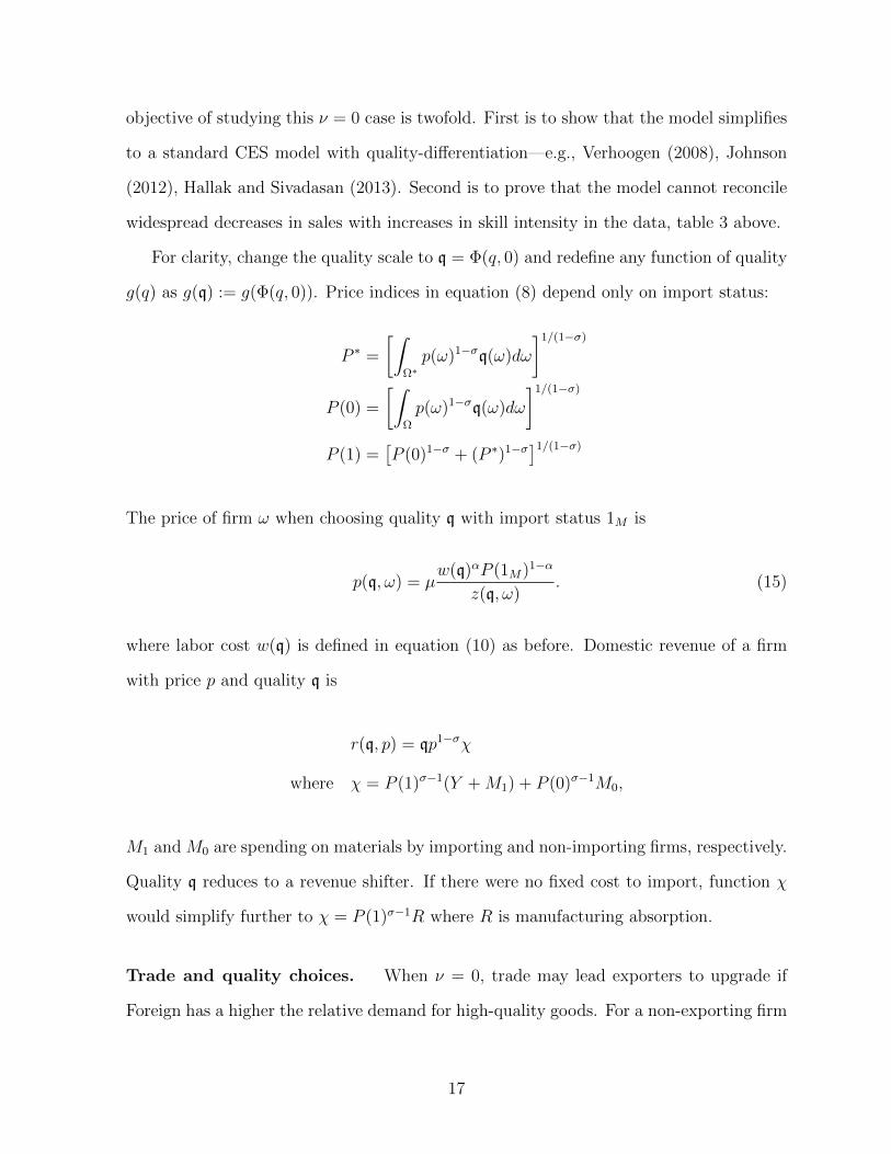
objective of studying this ν = 0 case is twofold. First is to show that the model simplifies
to a standard CES model with quality-differentiation—e.g., Verhoogen (2008), Johnson
(2012), Hallak and Sivadasan (2013). Second is to prove that the model cannot reconcile
widespread decreases in sales with increases in skill intensity in the data, table 3 above.
For clarity, change the quality scale to q = Φ(q, 0) and redefine any function of quality
g(q) as g(q) := g(Φ(q, 0)). Price indices in equation (8) depend only on import status:
P ∗ =
[∫Ω∗p(ω)1−σq(ω)dω
]1/(1−σ)
P (0) =
[∫Ω
p(ω)1−σq(ω)dω
]1/(1−σ)
P (1) =[P (0)1−σ + (P ∗)1−σ]1/(1−σ)
The price of firm ω when choosing quality q with import status 1M is
p(q, ω) = µw(q)αP (1M)1−α
z(q, ω). (15)
where labor cost w(q) is defined in equation (10) as before. Domestic revenue of a firm
with price p and quality q is
r(q, p) = qp1−σχ
where χ = P (1)σ−1(Y +M1) + P (0)σ−1M0,
M1 and M0 are spending on materials by importing and non-importing firms, respectively.
Quality q reduces to a revenue shifter. If there were no fixed cost to import, function χ
would simplify further to χ = P (1)σ−1R where R is manufacturing absorption.
Trade and quality choices. When ν = 0, trade may lead exporters to upgrade if
Foreign has a higher the relative demand for high-quality goods. For a non-exporting firm
17

ω, its profit when choosing quality q and import status 1M is:
π(q, ω) =r(q, p(q, ω))
σ− f(q)− 1MfM(ω)
The first order condition with respect to q is
r(q, p(q, ω))
qσ[1 + (1− σ)εpq]− f ′(q) ≥ 0 (16)
with equality whenever q > 0. The first term is the marginal benefit of upgrading quality
and f ′(q) is the marginal cost.
The term εpq = dp(q,ω)dq
qp(q,ω)
. In the price equation (15), labor cost w(q) is the only
endogenous variable that depends on quality q. Appendix B.3 shows that εpq increases
with the skill premium in the empirically-relevant case where higher-quality goods are
skill intensive.21 Then, if the trade liberalization increases the skill premium, the marginal
benefit of upgrading in equation (16) decreases unless revenue r(q, p(q, ω)) increases. The
firm upgrades only if its sales increase. Firms may downgrade even when sales increase
because the skill premium increases the relative cost of producing higher quality.
To summarize, for non-exporting firms—89% of firms on table 1 above—quality up-
grading when ν = 0 is equivalent to a skill-biased technical change that increases pro-
ductivity. Like R&D in Lileeva and Trefler (2010) and Bustos (2011), firms upgrade only
if their sales increase. So, this special case cannot reconcile increases in skill intensity
and skill premium with widespread decreases in sales in the data (table 3). This result
anticipates that parameter ν is critical for the general model to even qualitatively match
the changes in Colombian manufacturing following the trade liberalization.
21Appendix B.3 also proves non-exporters upgrade only if sales increase without differentiability.
18

3.2 Trade, Quality and Skills
A unilateral decrease in Home tariffs potentially increases the overall quality of Home
goods through several channels:
1. Selection. Importers and exporters expand production relative to lower-quality
firms. Although the liberalization is unilateral, it may increase exports if Home
quality increases or prices decrease—through a general equilibrium effect on Home
wages or through a decrease in the price of material inputs.
2. The production of higher quality exhibits increasing returns to scale due to fixed
cost f(q). Firms upgrade if their sales increase.
3. Demand for high-quality goods may be higher in Foreign. If exports increase,
exporters upgrade quality.
4. Foreign inputs may have higher quality than Home inputs. Trade decreases
importers’ relative cost of producing higher quality.
5. Magnification effect of domestic input market. Quality upgrading among
importers and exporters increases the domestic demand and supply of high-quality
goods. As a result, the relative cost of producing high quality decreases, and its
sales increase relative to low-quality goods. This effect impacts all firms—importers,
exporters and firms not engaged in international trade.
Because parameter estimates below imply that higher-quality goods are skill intensive,
demand for skilled workers increases with quality upgrading. Effects (1) through (4)
appear in the literature. There is only selection (1) in models where firms’ exogenous
productivity govern the demand for skill—e.g., Burstein and Vogel (2016), Blaum, Lelarge,
Peters (2016). Economies of scale (2) appear in Bustos (2011), Lileeva and Trefler (2010),
and Helpman, Itskhoki, Muendler, Redding (2016). Some combination of effects (3)
and (4) appears in models of offshoring—e.g., Feenstra and Hanson (1997) and Antras,
19

Garicano, Rossi-Hansberg (2006), Kugler and Verhoogen (2012)—and models with non-
homothetic preferences—Verhoogen (2008) and Faber (2014). Effect (5) is novel but does
not exist without at least a subset of direct effects (1) through (4).
It is an empirical question whether these theoretical mechanisms can explain the in-
crease in demand for skills following the trade liberalization. We estimate the model with
pre-liberalization data and use a counterfactual trade liberalization to study the ability of
these mechanisms in explaining overtime changes in the data. Although we cannot isolate
mechanisms that interact in general equilibrium, two special cases serve as benchmarks
in the counterfactuals. First, ν = 0 as in section 3.1. Effects (4) and (5) are shut down
because they both arise if the production of higher quality uses intensively high-quality
inputs. Second, quality is exogenous. Changes occur only through the reallocation of pro-
duction from low- to high-quality firms, not within firms. Effects (1)-(5) are all present in
this case because high-quality importers and exporters pass through their cost reductions
and increase input spending in proportion to sales.
4 Estimation procedure
We apply the method of simulated moments to pre-liberalization data. There are 51 mo-
ments and 18 parameters. We describe the parametrization in section 4.1, the simulation
in section 4.2, and moments and identification in section 4.3.
4.1 Parametrization
Table 4 summarizes the parameters. Assume all Foreign goods have the same price and
quality. We set wages of unskilled workers wu = 1, price of foreign goods p∗ = 1 for all
ω ∈ Ω∗, and consumer income Y = 1. These three normalizations correspond to setting
the numeraire, normalizing units with which prices are measured, and the size of the
20

Table 4: List of parameters
description model variable parametrization parameter
firm productivity z(q, ω) z(q) max0, z1(ω)[1 + z2(ω)q]z1 ∼ log-normal µ1, σ1
z2 ∼ normal with mean 0 σ2
z(q) = exp(z3q) z3
fixed cost of production f(q) = f1 + f2q f1, f2
fixed cost of importing fM(ω) ∼ log-normal µM , σMfixed cost of exporting fX(ω) ∼ log-normal µX , σXlabor demand shifters ΦL(s, q)/ΦL(u, q) equation (18) λ1, λ2
skill premium ws/wucomplementarity of input and output q νshifter in Foreign demand Q∗
size of Foreign market Y ∗
Quality of Foreign firms q∗
Measurement error in skills truncated logistic εLParameters not estimated: wu = Y = p∗ = 1, σ = 5, α = 0.7, t = 0.32, λ3, σL = 1.6.
labor force.22 The elasticity of substitution across goods σ enters only as an exponent of
z(q, ω) and is not separately identified from it. We take σ = 5 from Broda and Weinstein
(2006). Similarly, the elasticity of substitution between skilled and unskilled labor is not
separately identified from ΦL, and we take σL = 1.6 from Acemoglu and Autor (2010).
Section 7.2 experiments with other values for σ and σL. Average tariff on Colombian
manufactures in 1982-1988 is t = 32%. Labor share is α = 0.7.
We parameterize fixed costs f(q), fM(ω) and fX(ω), productivity z(q, ω), and labor
shifter ΦL. Production costs f(q) = f1 + f2q. Fixed costs of trade are log-normally
distributed with mean and variance parameters µM and σM for importing costs fM(ω),
and µX and σX for exporting costs fX(ω). Productivity is
z(q, ω) = z(q) max0, z1(ω)[1 + z2(ω)q], (17)
where z(q) = exp(z3q)
22We do not match number of employees, but sales relative to absorption. Doubling Y in the modeldoubles labor force L, sales and absorption, but it does not change the ratio of firm sales to absorption.
21

where z3 is a parameter, and z1(ω) and z2(ω) are independently drawn across firms. As-
sume z1(ω) has a log-normal distribution with mean parameter µ1 and variance parameter
σ1, and z2(ω) has a normal distribution with mean zero and variance σ2. Loosely speak-
ing, z1(ω) governs heterogeneity in firm sales, z2(ω) governs heterogeneity in the relation
between sales and skill intensity, while function z(q) is a common drift capturing the
systematic relation between skill intensity (quality) and prices.
For computational convenience, we make two normalizations that imply that z and
ΦL do not enter the firm’s problem (12).23 First, we set the aggregate labor cost in
equation (9) to w(q) = 1. This is without loss of generality because, with a Cobb-
Douglas production function, differences in labor costs across qualities in a cross-section
can be factored out into z(q).24 Second, demand equation (11) sets the overall revenue
gain from quality upgrading. This revenue has three components, z(q)σ−1, φ(q) and the
relative component[
exp(q−νq′)1+exp(q−νq′)
]from equation (5). Since we only have data on prices
and revenue, we cannot separately identify the common from the relative component,
and hence we set [z(q)]σ−1φ(q) = 1. In words, parameter z3 still governs the relationship
between prices and quality, but it does not govern revenue because changes in productivity
z are offset by changes in demand φ.
We parameterize the ratio ΦL(s,q)ΦL(u,q)
governing skill intensity in equation (4) as
ΦL(s, q)
ΦL(s, q) + ΦL(u, q)= λ3
exp(λ1 + λ2q)
1 + exp(λ1 + λ2q)(18)
where λ1, λ2 are parameters to be estimated. Skill intensity ls/l in equation (4) has the
shape of a logistic distribution function but is bounded above by λ3(ws)−σL . We pick λ3 so
that the skill intensity to produce foreign quality q∗ is 23%, the average of manufacturing
23Appendix C.1 details the computational convenience of this approach.24Prices are µ w(q)αP (1M )1−α
z(q) max0,z1(ω)[1+z2(ω)q] . Then, for any general w(q) in a cross-section, we can always
group the terms that are not firm-specific, set w(q) = 1 and redefine z(q) as the original z(q)w(q)−α. To
get w(q) = 1 for any ratio ΦL(s,q)ΦL(u,q) , we set ΦL(u, q) =
[w1−σLu + ΦL(s,q)
ΦL(u,q)w1−σLs
]−1
.
22

in the United States from Autor, Katz and Krueger (1998).25 Appendix C.2 experiments
with alternative specifications for ΦL(s,q)ΦL(u,q)
, including λ3 = 1.
The data report the share of white- and blue-collar workers, not their skill. Firm
sales, importing and exporting are much more correlated with wages than with white-
collar shares. Our interpretation is that firms observe skill better than we econometricians
and that wages reflect the true ranking of skill intensity. The estimation then uses the
ranking of wages to identify the ranking of quality, and white-collar shares to identify
shares of skilled workers. To simultaneously use all this information, we assume that some
unskilled workers are misclassified as white-collars. The share of misclassified workers is
independently drawn for each firm from a logistic distribution truncated in [0, ls/l] with
mean parameter zero and variance parameter εL.26 Remaining parameters are: Wages of
skilled workers ws, complementarity parameter ν, Foreign demand shifters Q∗ and Y ∗,
and quality of Foreign goods q∗.
4.2 Simulation
We simulate 100,000 firms. Each firm has a fixed vector of four independent standard
normal random variables. For each parameter guess, we transform these vectors into
productivity parameters z1(ω) and z2(ω), fixed costs fX(ω) and fM(ω). Firms may exit
or enter the market. If they enter, they choose quality from a grid with 200 choices
q ∈ [0, 10]. Together with the four choices on participation of international trade—to
import only, to export only, to import and export, or to do neither—firms have 801
discrete choices over which we iterate.27
25We take the share of college graduates, and average between 1980 and 1990 Census from table 1.26We assume that skilled workers are not misclassified as blue-collars for two reasons. In the data, the
wages of white-collars vary a lot more than that of blue-collars across firms, suggesting that the presenceof college graduates among blue-collars is not common. Second, if classification errors also applied toskilled workers, their predicted share would be close to the share of white-collar workers, 30%, and muchhigher than the share of college graduates in Colombia. Appendix C.2.2 details the calculation andidentification of these measurement errors.
27Results do not change when we increase the number of choices in the grid to 400 or if we change thevector of random variables.
23

Given these choices, the vector of prices P (q) is a fixed point calculated iteratively
for each quality level in the grid. Price indices are fixed points because they enter firms’
prices through material inputs. As in a standard CES model, the new guess of prices
in each iteration is a closed-form function of the old guess (equations (8) and (9)) and
convergence is fast. Given prices, demand function χ(q) is similarly calculated as a fixed
point of equation (11). Demand is a fixed point because firms’ demand for materials
depends on the demand they face. Given P and χ, we calculate the profit of each firm for
each of its 801 discrete choices and update its optimal choice. The equilibrium is attained
when no firm changes its choice.28
Implicitly, this procedure takes labor supply L(w) to equal the demand for labor, and
trade deficit D to equal the imports minus exports. The equilibrium is independent of
parameters z3, ws, λ1, λ2, εL, used to calculate moments related to labor and prices.
4.3 Moments and Identification
We use data pooled from 1982-1988. The list of moments is on table 5. Parameter
estimates minimize the squared distance between moments from the data and the model.
To capture qualitative aspects of the data, we weight moments with the identity matrix.
Results using the inverse of the variance of moments as weights are in section 7.2.29
Quality in the model is a latent variable that links a firm’s sales to its skill intensity,
average wage, prices of inputs and outputs, and import and export behavior. Identification
is possible because the model assumes that quality and sales are positively correlated.
The joint distribution of ranking of sales and wages helps identify the strength of this
correlation. Once the distribution of qualities in each quartile of sales is set, then the joint
distribution of sales and other firm variables allows for the identification of parameters
28To speed up the computation of P and χ, we define representative firms for each of the 800 discretechoices of producing firms, following Melitz (2003). See appendix C.1.1.
29The choice of weights affects efficiency, not bias. We multiply moments on the unconditional distri-bution of normalized sales by 0.01 so that their magnitude (table 7) is the same as other moments thatare measured in shares, not logs. The main difference in the appendix is that moments related to pricesare not matched because their weights are much smaller than the weight on other moments.
24

Table 5: List of moments
# of moments parameter∗∗
• 10%, 25%, 50%, 75%, 90% of the unconditional distribution of...... log(normalized domestic sales)∗ 5 µ1, σ1
... share of white-collar workers in employment 5 λ1, λ2
• share of firms in the nth quartile of domestic sales and the mth quartileof average wages for n,m = 1, ..., 4 16 σ2, f2
• By quartile of domestic sales, ...... average share of white-collar workers 4 εL... share of plants importing 4 µM , σM... share of plants exporting 4 µX , σX... average spending on imported inputs/total spending on materials 4 µ1, q∗
... average export sales/total sales 4 Y ∗, Q∗
• coefficient of regression of output prices on white-collar shares† 1 z3
• coefficient of regression of input prices on white-collar shares† 1 ν• average wage of white collars/average wage of blue collars 1 ws/wu• aggregate share of white-collar workers 1 εL• yearly exit rate 1 f1
total 51
† Price regressions in the data include fixed effects for year, product, and sector of the purchasing firm.∗ Normalized sales are sales divided by total manufacturing absorption. We calculate absorption in thedata as total sales in our manufacturing survey plus Colombian manufacturing imports minus exportsfrom Feenstra et al (2005). To get sales in the model, we weight each firm in the model in proportion tothe number of plants in the data. ∗∗ Parameters are all jointly determined. The column links momentsto parameters that they best help identify.
25

relating quality to skills, import and export behavior. The critical parameter ν linking
input and output qualities is identified from price regressions.
We elaborate this identification argument in steps. For guidance, the last column of
table 5 lists parameters whose identification is associated to moments on the first column.
1. Unconditional distribution of sales identifies the mean and spread of firm produc-
tivity µ1, σ1. Parameter µ1 governs mean sales and σ1 its spread. Normalized
sales depends negatively on import intensities, and so parameter µ1 simultaneously
governs sales and average import intensity.
2. The fixed cost to enter f1 governs the exit rate.30
3. The model always generates a positive correlation between sales and quality because
demand is increasing in quality. Since all firms of the same quality have the same
average wage, the positive correlation between sales and wages in the data imply
that skill intensity increases in quality and that the ranking of wages is identical to
the ranking of quality in the model.31
The tightness of the relation between sales and wages identifies parameters σ2, f2
governing quality choices. If the fixed cost to produce higher quality f2 were large,
then small firms would never have a high wage rank. If firms did not differ in their
comparative advantage in producing quality, σ2 ≈ 0, large firms would generally
produce higher quality due to returns to scale. Parameters σ2 and f2 also ensure
that quality choices lie in the grid [0, 10]. The results depend more on the ranking
than the value of quality, and so this grid choice normalizes the quality scale.32
4. The joint distribution between sales and quality from step 3 contains information
30We do not observe the share of firms that exit upon entry, and we take this share to match thehistorical yearly exit rate.
31We target only ranking of wages because a model with perfect labor markets and only two skill levelscannot generate the variation of wages in data.
32Monte Carlo simulations in appendix E show that the spread of quality levels is well identified(through imports and exports below) but not small shifts in its location. Nothing at all changes if we usea larger quality grid, [0, 15] or [0, 20].
26

on the distribution of quality in each quartile of sales. We can then identify the
remaining parameters because, in the model, all firms of the same quality value
labor and material inputs equally.
• Skills. The tighter relation between sales and wages relative to sales and
white-collar shares informs measurement error εL. Given this error, the skill
premium ws/wu governs measured skill premium wwhite-collars/wblue-collars, and
parameters λ1 and λ2 in equation (18) govern the level and spread of the
distribution of skill intensity.33
• Input and output quality. We match the coefficients from regressing
output price on skill intensity, and separately, input prices on skill intensity
(table 9 below). The coefficient on the regression of output prices and skill
intensity identifies the rate at which average firm productivity decreases in
quality, parameter z3 in equation (17). This moment is critical because, given
the relation between output price and skill intensity, the coefficient on the
input-price regression informs the model of the extent to which skill-intensive
firms buy more inputs from other skill intensive firms—governed in the model
by parameter ν. If firms with output quality q only used inputs of quality q,
then the coefficients in the input- and output-price regressions would be equal.
But the coefficient is smaller in the input-price regression, suggesting that firms
spread their purchases over various quality levels. If ν = 0, the coefficient on
the input-price regression would be zero.
• International trade. The share of firms importing and exporting by quar-
tile of sales identifies the distributions of the fixed costs of international trade
and their variance—parameters µM , σM , µX , σX . Conditional on participation,
firms of the same quality have the same import and export intensity. Parame-
33See also appendix C.2. It discusses other parametrizations of skill intensity, and it shows the worseningfit of the model, in and out of sample, when there is no measurement error.
27

Figure 1: Distribution of quality (density)
ter Y ∗ governs average export intensity, and Q∗ governs how export intensity
increases with sales. Similarly, the quality of foreign inputs q∗ governs how
import intensity increases with sales. Trade also helps identify quality choices,
parameters f2 and σ2 above, because import and export intensities would not
vary across firms if the spread of quality levels were too small.
Appendix E presents Monte Carlo simulations to check for identification. We gener-
ate data with parameter estimates and re-run the optimization algorithm starting with
random initial guesses. In all simulations the algorithm converged to values very close to
the original estimates.
5 Estimation Results
5.1 Within-sample results
Results within sample are in section 5.1 and results out of sample are in section 5.2.
All these results use pre-liberalization data. Estimated parameters are on table 6. The
distribution of quality in figure 1 has multiple peaks due to discrete choices of trading.
Foreign has a higher relative demand and supply of high-quality goods—Q∗ = 4.2 > 0
and q∗ = 12 is higher than even the highest Home quality, q = 9.4. Production of higher-
28

Table 6: Parameter estimates
parameter estimate std. error parameter estimate std. error
µ1 -0.055 0.007 σX 3.63 0.06σ1 0.556 0.002 λ1 -8.22 1.26σ2 3.3E-03 3.9E-04 λ2 1.77 0.34z3 -0.59 0.08 ws/wu 2.84 0.03f1 9.0E-04 3.8E-05 q∗ 11.8 0.6f2 4.7E-05 4.7E-06 Y ∗ 0.05 0.0017µM -3.96 0.05 Q∗ 4.16 0.29σM 2.60 0.03 πL 0.15 0.002µX -0.32 0.07 ν 1.07 0.01
quality goods is intensive in high-quality material inputs ν = 1.1 > 0 and in skilled labor
λ2 = 1.8 > 0. Average fixed cost paid for importing is about $29,000, and for exporting,
it is $108,000 in 2009 US dollars—in line with the literature.34 Exit upon entry is 10% in
the data and 11% in the model.
The model fits the data well. On table 7 are the unconditional distributions of sales
and skill intensity. Data figures of table 8 are repeated from table 1 above. In the data
and model, firms in the upper quartiles of sales are skill intensive, more likely to import
and export, and they export a higher share of their output and import a higher share
of their inputs. Sales and wages are positively correlated in figure 2.35 The targeted
moments, share of firms in each bin, are in appendix C.7. A small estimate of f2, the
slope of fixed cost f(q), explains the existence of small firms with high wages in the model,
and it implies that economies of scale is not an important determinant of quality.
Price regressions on table 9 suggest that high-quality firms disproportionately source
inputs from other high-quality firms. The input price regressions are repeated from table
2 above. In the data and model, a 10% point increase in skill intensity is associated
with an increase of 4% in output price and 2% in input price. Compared to other firms
34See Das, Roberts, Tybout (2007). We calculate these costs through the ratio of average sales to fixedcosts assuming that average sales is the same as in the data—average sales in the model are proportionalto Y = 1. Costs are large because they reflect expected profits from international trade.
35For visualization, the data figure has only the 7,130 firms in 1988, and the model figure plots also7,130 firms, randomly selected from the 100,000 firms simulated.
29

Table 7: Unconditional distribution of sales and measured skill intensity
10th 25th 50th 75th 90th
normalized domestic sales, in logsdata -12.6 -11.9 -11.0 -9.8 -8.4model -13.5 -12.6 -11.3 -9.9 -8.6white-collar shares, in %data 5.9 13 22 34 50model 6.2 12 21 34 49price-adjusted sales q (out of sample)data -2.9 -1.5 0.0 1.4 3.0model -1.4 -0.9 0.0 0.8 2.7
Table 8: Joint distributions of sales with other characteristics (in %)
quartiles of domestic sales1 2 3 4 (largest)
share of white-collar workersdata 20 22 26 34model 22 24 26 29
share of importing plantsdata 7.4 12 25 58model 4.1 12 27 58
spending on imported materials/totaldata 1.9 3.7 7.6 19model 1.0 3.4 8.2 19
share of exporting plantsdata 2.7 3.6 8.8 28model 2.1 5.0 10 25
export sales/total salesdata 1.4 1.0 1.6 2.6model 0.3 0.8 1.6 4.1
price-adjusted sales q (logs, out of sample)data -1.2 -0.3 0.2 0.9model -1.4 -0.3 0.3 1.5
in the model, firms in the upper quartile of quality source 10% more of their domestic
inputs from other high-quality firms (not on table). Importers and exporters account for
more than 70% of purchases of domestic inputs and sales in the data and model.36 Large
36We do not directly observe firm-to-firm sourcing in our data. Importers’ and exporters’ total spendingon materials is 71% of all firms’ spending on materials. Importers and exporters’ domestic sales are 76%of manufacturing absorption of inputs and final goods.
30
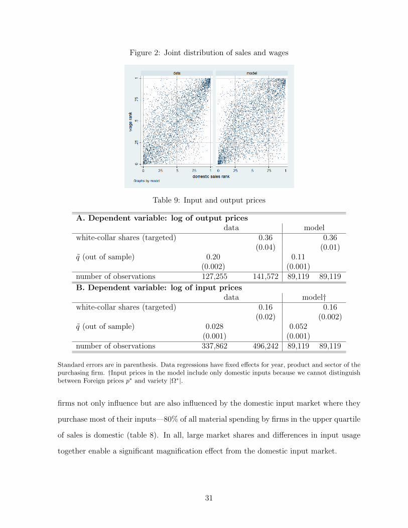
Figure 2: Joint distribution of sales and wages
Table 9: Input and output prices
A. Dependent variable: log of output pricesdata model
white-collar shares (targeted) 0.36 0.36(0.04) (0.01)
q (out of sample) 0.20 0.11(0.002) (0.001)
number of observations 127,255 141,572 89,119 89,119
B. Dependent variable: log of input pricesdata model†
white-collar shares (targeted) 0.16 0.16(0.02) (0.002)
q (out of sample) 0.028 0.052(0.001) (0.001)
number of observations 337,862 496,242 89,119 89,119
Standard errors are in parenthesis. Data regressions have fixed effects for year, product and sector of thepurchasing firm. †Input prices in the model include only domestic inputs because we cannot distinguishbetween Foreign prices p∗ and variety |Ω∗|.
firms not only influence but are also influenced by the domestic input market where they
purchase most of their inputs—80% of all material spending by firms in the upper quartile
of sales is domestic (table 8). In all, large market shares and differences in input usage
together enable a significant magnification effect from the domestic input market.
31

Table 10: Aggregate skill intensity and premium
measured skill (targeted) data modelskill intensity Lwhite/L (in %) 29 32skill premium wwhite/wblue 1.59 1.59
unobserved skill (out of sample) Colombian avg.† modelskill intensity Ls/L (in %) 8.5 11.6skill premium ws/wu 1.8 - 2.6 2.8† The Colombian average is from Attanasio, Goldberg, Pavcnik (2004).
5.2 Out-of-sample
We present out-of-sample moments on measures of quality and skill intensity used to
interpret counterfactuals of section 6. We also use pre-liberalization data to reject two
special cases of the model used as benchmarks.
Skill measure. The data do not report the education of workers, but predictions on
aggregate skill intensity and premium are well aligned with the Colombian household sur-
vey used by AGP on table 10. Between 1982 and 1988, about 8.5% of heads of households
had a college degree and the skill premium was ws/wu = 2.6 for university to elementary
school and 1.8 for university to secondary school. Our estimated skill intensity is 11.6%
and skill premium is 2.8.
Quality measure. The value of quality q in the model does not have an economic
interpretation. Define price-adjusted sales as
q(ω) = log r(ω)− (1− σ) log p(ω)− [log r − (1− σ) log p] (19)
= logχ(q(ω))− logχ
where r(ω) is the domestic revenue of firm ω, and the second term in both lines (with a bar)
is the average of the first term across firms. Since χ is strictly increasing, q is a monotonic
transformation of q that is observable and has a straightforward interpretation: A firm
32
has a higher q if it sells more after adjusting for prices. Following Khandelwal (2010),
we define q in the data as firm×time effects estimated over the residual log(revenue) −
(1 − σ) log(p), where this residual is calculated separately for each product-plant-year
combination and deviated from product fixed effects.37 Appendix A.3 shows that q is
correlated with wages, skill intensity, probability of importing and exporting, import and
export shares—as predicted by the model.
The estimation uses skill intensity and wages to identify quality. Tables 7-9 check
the out-of-sample predictions of the model when we substitute these moments on skills
with q and compare them to data. The reasonable fit of the model is reassuring, but we
do not use price-adjusted sales q directly in the estimation for two main reasons. First,
measurement error in prices biases regressions on table 9. Most important on panel A,
simultaneity biases upward the coefficient from regressing output prices on q because the
dependent variable, output prices, is used to calculate the independent variable q. On
panel B, attenuation biases the coefficient on q downward, because q is measured with
error. Second, price-adjusted sales q are not comparable over time because sales and
input costs change with the trade liberalization even if quality does not change (function
χ is endogenous). So, directly targeting skills makes sense as increases in skill intensity
and skill premium from the mid-1980s to 1994 are key evidence of quality upgrading in
the data. For robustness, section 7.2 re-estimates the model substituting all moments on
skills with the corresponding moments on q.
Special case I: ν = 0. The hypothesis ν = 0 is clearly rejected by estimated ν = 1.1
with standard error 0.01. Qualitatively when ν = 0, input prices do not vary with skill
intensity or price-adjusted sales—contradicting table 9B. Also, importing does not depend
on skill-intensity after controlling for sales. In contrast, table 11 shows that skill-intensive
37The only difference from Khandelwal (2010) is that he uses variation across different exportingcountries, while we use variation across firms within products. In the data, we use total revenue becausewe do not observe domestic revenue separately by product category where prices are comparable. In themodel, the correlation between q calculated with domestic or with total revenue is 0.999.
33
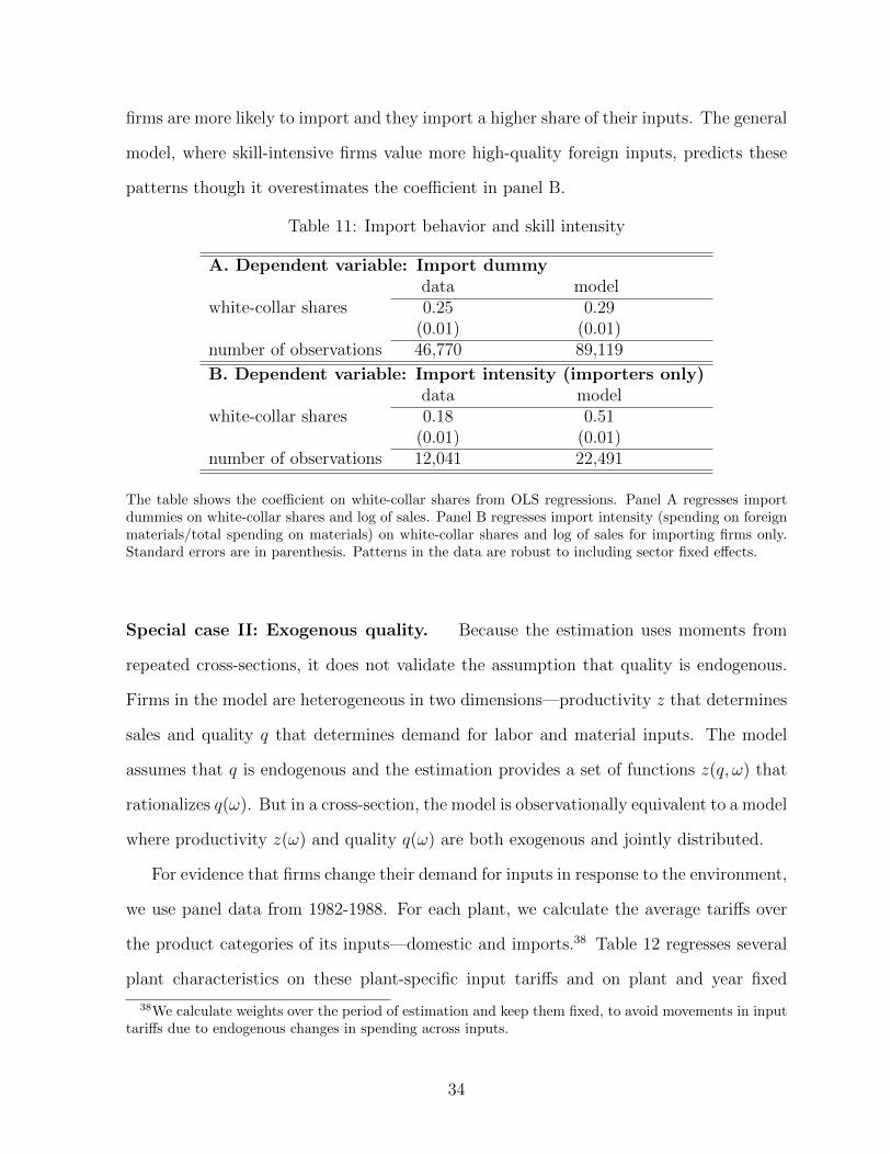
firms are more likely to import and they import a higher share of their inputs. The general
model, where skill-intensive firms value more high-quality foreign inputs, predicts these
patterns though it overestimates the coefficient in panel B.
Table 11: Import behavior and skill intensity
A. Dependent variable: Import dummydata model
white-collar shares 0.25 0.29(0.01) (0.01)
number of observations 46,770 89,119
B. Dependent variable: Import intensity (importers only)data model
white-collar shares 0.18 0.51(0.01) (0.01)
number of observations 12,041 22,491
The table shows the coefficient on white-collar shares from OLS regressions. Panel A regresses importdummies on white-collar shares and log of sales. Panel B regresses import intensity (spending on foreignmaterials/total spending on materials) on white-collar shares and log of sales for importing firms only.Standard errors are in parenthesis. Patterns in the data are robust to including sector fixed effects.
Special case II: Exogenous quality. Because the estimation uses moments from
repeated cross-sections, it does not validate the assumption that quality is endogenous.
Firms in the model are heterogeneous in two dimensions—productivity z that determines
sales and quality q that determines demand for labor and material inputs. The model
assumes that q is endogenous and the estimation provides a set of functions z(q, ω) that
rationalizes q(ω). But in a cross-section, the model is observationally equivalent to a model
where productivity z(ω) and quality q(ω) are both exogenous and jointly distributed.
For evidence that firms change their demand for inputs in response to the environment,
we use panel data from 1982-1988. For each plant, we calculate the average tariffs over
the product categories of its inputs—domestic and imports.38 Table 12 regresses several
plant characteristics on these plant-specific input tariffs and on plant and year fixed
38We calculate weights over the period of estimation and keep them fixed, to avoid movements in inputtariffs due to endogenous changes in spending across inputs.
34

Tab
le12
:W
ithin
-firm
chan
ges
and
input
tari
ffs,
pan
eldat
a19
82-1
988
OL
Sw
hit
e-co
llar
aver
age
pri
cep
rice
imp
ort
imp
ort
exp
ort
exp
ort
share
sw
age
ofin
pu
tsof
outp
ut
qd
um
my
shar
ed
um
my
shar
e(1
)(2
)(3
)(4
)(5
)(6
)(7
)(8
)(9
)in
pu
tta
riff
s ω-0
.005
58
-0.0
825
0.05
51-0
.117
-0.1
12-0
.032
1-0
.015
9-0
.039
3-0
.006
02(0
.009
05)
(0.0
205)
(0.0
191)
(0.0
218)
(0.1
70)
(0.0
189)
(0.0
0761
)(0
.015
8)(0
.004
46)
obse
rvati
on
s44,2
9644
,289
44,4
1143
,053
26,7
7444
,452
44,4
5044
,452
44,4
20R
-squ
are
d0.
789
0.86
10.
762
0.82
70.
742
0.83
70.
858
0.77
60.
815
pla
nt
fixed
effec
tye
sye
syes
yes
yes
yes
yes
yes
yes
year
fixed
effec
tye
sye
syes
yes
yes
yes
yes
yes
yes
Dep
Mea
n.2
556.
478
1.13
11.
136
0.2
57.0
8.1
08.0
19D
epsd
.187
.521
.448
.485
2.46
7.4
37.1
89.3
11.0
99In
dep
Mea
n0.3
830.
383
0.38
30.
383
0.38
30.
383
0.38
30.
383
0.38
3In
dep
sd0.1
530.
153
0.15
30.
153
0.15
30.
153
0.15
30.
153
0.15
3
IV:
On
e-p
eri
od
lagged
inp
ut
tari
ffs ω
are
the
inst
rum
ents
for
inp
ut
tari
ffs ω
.w
hit
e-co
llar
aver
age
pri
cep
rice
imp
ort
imp
ort
exp
ort
exp
ort
share
sw
age
ofin
pu
tsof
outp
ut
qd
um
my
shar
ed
um
my
shar
e(1
)(2
)(3
)(4
)(5
)(6
)(7
)(8
)(9
)in
pu
tta
riff
s ω-0
.0737
-0.0
801
-0.0
916
-0.3
86-0
.899
-0.1
16-0
.037
1-0
.142
-0.0
489
(0.0
261)
(0.0
572)
(0.0
538)
(0.0
609)
(0.4
86)
(0.0
529)
(0.0
211)
(0.0
446)
(0.0
116)
obse
rvati
on
s37,0
8937
,082
37,1
9136
,070
22,5
4137
,220
37,2
1837
,220
37,1
96R
-squ
are
d0.
798
0.86
80.
787
0.84
20.
760
0.85
00.
873
0.79
30.
846
pla
nt
fixed
effec
tye
sye
syes
yes
yes
yes
yes
yes
yes
year
fixed
effec
tye
sye
syes
yes
yes
yes
yes
yes
yes
Part
ial
equ
ilib
riu
meff
ects
of
inp
ut
tari
ffs
inm
od
el
gen
eral
mod
el-0
.022
-0.0
36-0
.081
-0.2
97-1
.21
-0.0
49-0
.104
-0.0
04-0
.001
3ex
ogen
ou
squ
alit
y0
00.
033
0.01
00
-0.0
70-0
.082
-0.0
004
-0.0
0007
*We
can
not
dis
tin
guis
hb
etw
een
fore
ign
pri
cesp∗
an
dva
riet
ies.
We
pro
xy
for
chan
ges
inin
pu
tp
rice
sin
mod
elas
(1-i
mp
ort
share
)*∆
dom
esti
cin
pu
tp
rice
s+
(im
por
tsh
are*
∆in
pu
tta
riff
).S
tan
dar
der
rors
inp
are
nth
esis
.
35
effects. Panel A has OLS results, and panel B instruments input tariffs with their lagged
values to partly address the concern that firms may lobby for lower input tariffs.39 Prior
to the liberalization, tariff changes were small and often temporary. Average tariffs on
manufacturing inputs were 27% in 1982, 43% in 1984, and 27% in 1988.
In our preferred IV panel, an increase in tariffs is associated with a decrease in white-
collar shares, wages (not significant), input and output prices, and export participation.
The signs of coefficients are all consistent with the estimated model where input tariffs
decrease firm quality, demand for skilled labor, the quality of material inputs, and export
sales. The negative coefficient on input and output prices is particularly surprising because
input tariffs directly increase input prices.
Since tariff changes between 1982 and 1988 were relatively small and our input tariffs
are firm-specific, we interpret the coefficients as the partial-equilibrium effects of input
tariffs on firms. The last two rows of the table report the average response of firms
when we individually decrease their input tariffs so that import probability and intensity
increase on average 7.7%, the average of coefficients on columns (6) and (7) in the IV
specification.40 In the general model, white-collar shares increase by 2.2% points, input
prices by 8.1% points, output prices by 30% and price-adjusted sales q by 121%. The
corresponding numbers in the data 7.4%, 9.2%, 39% and 90% (columns 1, 3, 4, 5) have
similar magnitudes. In contrast, when quality is exogenous, labor-related variables do not
move with tariffs, and input and output prices always increase with tariffs.
Table 12 complements mounting evidence from the literature that imported inputs
and the development of a domestic input market increase technology, product quality and
variety.41 Although alternative explanations may be put forth, the table is consistent
39Another common instrument, the initial level of tariffs, can only be used in periods of large tradeliberalizations, where the level and standard deviation of tariffs are reduced. Endogeneity is not an issuefor the level of tariffs, only for changes if firms lobbying efforts vary with time.
40The model’s decrease in tariff is 10%. When quality is endogenous, import intensity rises faster withtariffs in the model than in pre-liberalization data, possibly because tariff changes were temporary.
41See Goldberg, Khandelwal, Pavcnik, Topalova (2009, 2010), Bøler, Moxnes and Ultveit-Moe (2016),Halpern, Koren and Szeidl (2015). Eslava et al. (2015), Kee (2015), and Kee and Tang (2016) providesupport for indirect effects of trade through domestic inputs.
36

with the effects of imported inputs on within-firm outcomes in the general model and
inconsistent with the exogenous-quality hypothesis.
6 Counterfactual Trade Liberalization
We study the effect of observed changes in international trade on quality and demand for
skills in the model, under different specifications. Robustness checks in section 7.2 confirm
general magnitudes and qualitative patterns. In the data, effects of trade are confounded
with other shocks, secular trends, and normal firm and business-cycle dynamics. But
because international trade was a major reform between mid 1980s and 1994, the data
offer a guideline for the magnitude of changes and its heterogeneous effect on firms.
We exogenously decrease tariffs from 32% to 12%, the Colombian manufacturing av-
erages in 1982-1988 and in 1994, respectively. Although tariff cuts endogenously increase
imports and exports in the model, we cannot predict changes in trade volumes without
additional information on non-tariff barriers, exchange rates, domestic and foreign growth
rates, etc. So, we allow Foreign pre-tariff price p∗ and market-size Y ∗ to change to ex-
actly match changes in imports and exports in the data. Combining aggregate trade data
from Feenstra et al. (2005) with sales from the Manufacturing Survey, we estimate that
between the mid 1980s and 1994, manufacturing imports expanded from 16.2% to 28.1%
of manufacturing absorption, and exports expanded from 4.5% to 7.5%. We match this
expansion of 11.8% points in imports and 3.0% points in exports.
Cross-sectional data contain no information on the elasticity of labor supply, only
on the supply of labor given wages. Between the mid 1980s and 1994 in Colombia, the
skill premium and skill intensity increased in manufacturing, suggesting that labor is
imperfectly elastic.42 But to clearly understand the workings of the model, we consider
two extreme cases: Labor is perfectly elastic and wages (wu, ws) do not change in section
42To estimate the elasticity of labor in and out of manufacturing, one would need to observe the skillpremium in manufacturing relative to non-manufacturing sectors.
37
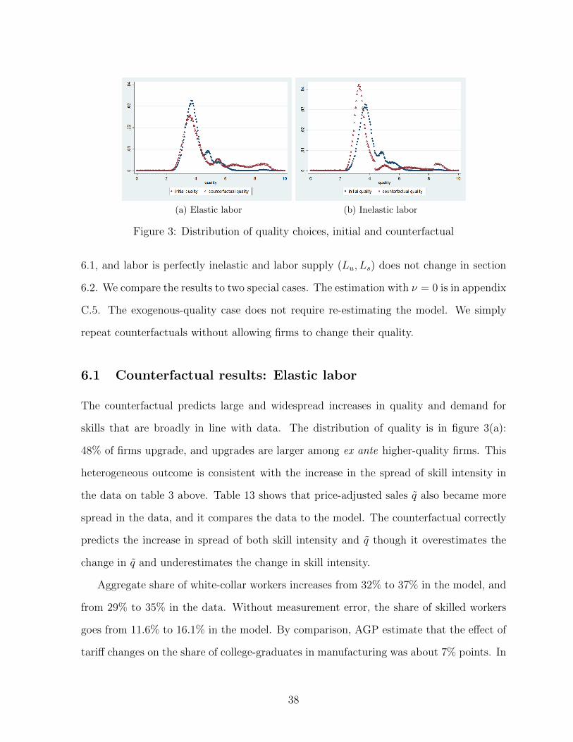
(a) Elastic labor (b) Inelastic labor
Figure 3: Distribution of quality choices, initial and counterfactual
6.1, and labor is perfectly inelastic and labor supply (Lu, Ls) does not change in section
6.2. We compare the results to two special cases. The estimation with ν = 0 is in appendix
C.5. The exogenous-quality case does not require re-estimating the model. We simply
repeat counterfactuals without allowing firms to change their quality.
6.1 Counterfactual results: Elastic labor
The counterfactual predicts large and widespread increases in quality and demand for
skills that are broadly in line with data. The distribution of quality is in figure 3(a):
48% of firms upgrade, and upgrades are larger among ex ante higher-quality firms. This
heterogeneous outcome is consistent with the increase in the spread of skill intensity in
the data on table 3 above. Table 13 shows that price-adjusted sales q also became more
spread in the data, and it compares the data to the model. The counterfactual correctly
predicts the increase in spread of both skill intensity and q though it overestimates the
change in q and underestimates the change in skill intensity.
Aggregate share of white-collar workers increases from 32% to 37% in the model, and
from 29% to 35% in the data. Without measurement error, the share of skilled workers
goes from 11.6% to 16.1% in the model. By comparison, AGP estimate that the effect of
tariff changes on the share of college-graduates in manufacturing was about 7% points. In
38

Table 13: Changes in the distributions of sales and skill intensity, model and data
percentiles10% 25% 50% 75% 90% mean
ln(normalized sales), final - initialdata -0.07 -0.08 -0.04 0.004 -0.07 -0.08elastic labor -0.04 -0.09 -0.11 -0.11 -0.10 -0.07inelastic labor -0.07 -0.10 -0.12 -0.11 -0.10 -0.08
white-collar shares, final - initial† (in %)data 3.2 4.2 6.0 9.2 14 6.4elastic labor 0.3 1.0 2.7 3.0 3.2 4.4inelastic labor -1.4 -1.6 -0.9 -0.6 -0.4 0
distribution of q, final - initial∗
data -0.4 -0.2 0.0 0.2 0.4 -elastic labor -0.9 -0.8 -0.3 0.4 3.1 -inelastic labor -0.4 -0.5 -0.6 -0.8 1.4 -
Final period refers to counterfactual in the model and 1994 in the data. We calculate the percentilesof the distributions before and after the counterfactual, and subtract the initial percentages from thecounterfactual ones. † Changes in total skill intensity are larger than percentile changes because laborshifts from less to more skill-intensive firms. See appendix C.6. ∗ Price-adjusted sales q(ω) are demeanedpre- and post-liberalization.
sum, the predicted increase in skill intensity of around 4.4% points—measured in white-
collar shares or college-graduates—is not far from data. But the model, with perfectly
elastic labor and no change in skill premium, underestimates the overall rise in demand
for skills considering that the skill premium increased by 11% in the data. The decrease in
normalized sales, of around 8%, is similar in the data and model because it is mechanically
linked to changes in imports and exports. In the model, 3% of active firms exit.
Like in the data, counterfactual price-adjusted sales q do not convey overall quality
changes because demand function χ is endogenous. To quantify quality changes, define
∆q(ω) = logχ0(q1(ω))− logχ0(q0(ω)) (20)
where subscript 0 refers to the estimated model and 1 refers to counterfactual. In words,
∆q(ω) is the hypothetical change in price-adjusted sales q if firm ω offered counterfactual
quality q1(ω) in period 0. Average ∆q is 0.79, compared to a standard deviation of q0 in
39
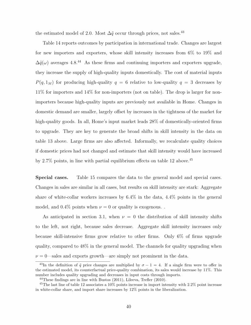
the estimated model of 2.0. Most ∆q occur through prices, not sales.43
Table 14 reports outcomes by participation in international trade. Changes are largest
for new importers and exporters, whose skill intensity increases from 6% to 19% and
∆q(ω) averages 4.8.44 As these firms and continuing importers and exporters upgrade,
they increase the supply of high-quality inputs domestically. The cost of material inputs
P (q, 1M) for producing high-quality q = 6 relative to low-quality q = 3 decreases by
11% for importers and 14% for non-importers (not on table). The drop is larger for non-
importers because high-quality inputs are previously not available in Home. Changes in
domestic demand are smaller, largely offset by increases in the tightness of the market for
high-quality goods. In all, Home’s input market leads 28% of domestically-oriented firms
to upgrade. They are key to generate the broad shifts in skill intensity in the data on
table 13 above. Large firms are also affected. Informally, we recalculate quality choices
if domestic prices had not changed and estimate that skill intensity would have increased
by 2.7% points, in line with partial equilibrium effects on table 12 above.45
Special cases. Table 15 compares the data to the general model and special cases.
Changes in sales are similar in all cases, but results on skill intensity are stark: Aggregate
share of white-collar workers increases by 6.4% in the data, 4.4% points in the general
model, and 0.4% points when ν = 0 or quality is exogenous. .
As anticipated in section 3.1, when ν = 0 the distribution of skill intensity shifts
to the left, not right, because sales decrease. Aggregate skill intensity increases only
because skill-intensive firms grow relative to other firms. Only 6% of firms upgrade
quality, compared to 48% in the general model. The channels for quality upgrading when
ν = 0—sales and exports growth—are simply not prominent in the data.
43In the definition of q price changes are multiplied by σ − 1 = 4. If a single firm were to offer inthe estimated model, its counterfactual price-quality combination, its sales would increase by 11%. Thisnumber includes quality upgrading and decreases in input costs through imports.
44These findings are in line with Bustos (2011), Lileeva, Trefler (2010).45The last line of table 12 associates a 10% points increase in import intensity with 2.2% point increase
in white-collar share, and import share increases by 12% points in the liberalization.
40
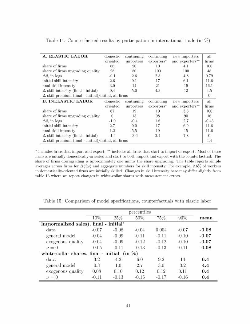
Table 14: Counterfactual results by participation in international trade (in %)
A. ELASTIC LABOR domestic continuing continuing new importers alloriented importers exporters∗ and exporters∗∗ firms
share of firms 66 20 10 4.1 100share of firms upgrading quality 28 80 100 100 48∆q, in logs -0.1 2.6 2.3 4.8 0.79initial skill intensity 2.6 9.1 17 6.1 11.6final skill intensity 3.0 14 21 19 16.1∆ skill intensity (final - initial) 0.4 5.0 4.3 12 4.5∆ skill premium (final - initial)/initial, all firms 0
B. INELASTIC LABOR domestic continuing continuing new importers alloriented importers exporters∗ and exporters∗∗ firms
share of firms 67 19 10 3.3 100share of firms upgrading quality 0 15 98 90 16∆q, in logs -1.0 -0.4 1.6 2.7 -0.43initial skill intensity 2.7 9.0 17 6.9 11.6final skill intensity 1.2 5.5 19 15 11.6∆ skill intensity (final - initial) -1.4 -3.6 2.4 7.8 0∆ skill premium (final - initial)/initial, all firms 4.4
∗ includes firms that import and export. ∗∗ includes all firms that start to import or export. Most of thesefirms are initially domestically-oriented and start to both import and export with the counterfactual. Theshare of firms downgrading is approximately one minus the share upgrading. The table reports simpleaverages across firms for ∆q(ω) and aggregate numbers for skill intensity. For example, 2.6% of workersin domestically-oriented firms are initially skilled. Changes in skill intensity here may differ slightly fromtable 13 where we report changes in white-collar shares with measurement errors.
Table 15: Comparison of model specifications, counterfactuals with elastic labor
percentiles10% 25% 50% 75% 90% mean
ln(normalized sales), final - initial∗
data -0.07 -0.08 -0.04 0.004 -0.07 -0.08general model -0.04 -0.09 -0.11 -0.11 -0.10 -0.07exogenous quality -0.04 -0.09 -0.12 -0.12 -0.10 -0.07ν = 0 -0.05 -0.11 -0.13 -0.13 -0.11 -0.08
white-collar shares, final - initial† (in %)data 3.2 4.2 6.0 9.2 14 6.4general model 0.3 1.0 2.7 3.0 3.2 4.4exogenous quality 0.08 0.10 0.12 0.12 0.11 0.4ν = 0 -0.11 -0.13 -0.15 -0.17 -0.16 0.4
41

When quality is exogenous and labor is elastic, firms do not change their skill intensity,
but the exit of 3% of firms slightly shifts upward the distribution of skill intensity. Changes
in aggregate skill intensity come only through reallocation of production, not within-firms.
The scope for reallocation is limited because large, skill-intensive firms account for most
employment in pre-liberalization data. For example, the average share of white-collar
workers is 29% in the aggregate and 30.5% in firms with sales above median. So, even
if all production were reallocated to these larger firms, aggregate skill intensity would
change by 1.5% points. There is no evidence of such radical reallocation of production.
In the general model, the penetration of high-quality foreign inputs increases domestic
quality and thereby increases Home exports to Foreign. This effect is so large that to
match the observed export expansion, the model predicts a decrease in Y ∗ of 11%. This
decrease may be interpreted as a real appreciation of Home currency because it decreases
the size of the Foreign market relative to Home prices and absorption. It exactly matches
the 11% appreciation of Colombian pesos between 1988 and 1994. In contrast, special
cases with ν = 0 or exogenous quality both predict an increase in Y ∗ of 7%. Similar to
trade models without intermediate inputs, these special cases require a real depreciation
(a fall in domestic wages) for exports to increase in unilateral liberalizations.46
6.2 Counterfactual results: Inelastic labor
When the supply of labor to manufacturing is fixed, the skill premium ws/wu increases
by 4.4%, from 2.84 to 2.96, confirming that trade significantly increases the demand for
skills in the model but by less than in the data where the skill premium increased by 11%.
With inelastic labor, trade has an ambiguous effect on the relative cost of high-quality
goods. Quality upgrading among importers and exporters decreases the relative price
of high-quality material inputs as before. But the skill premium increases the relative
46The general model and exogenous-quality case predict that pre-tariff price of foreign goods fall byabout 7% which is consistent with the removal of non-tariff barriers. When ν = 0, p∗ practically doesnot change with the counterfactual (it increases by 0.1%). Parameters p∗ and Y ∗ may be influenced bynumerous other factors, such as differential growth rates, foreign changes in trade policy.
42

cost of labor inputs. Quantitatively, the first effect dominates in the upper tail of the
quality distribution, while the second effect dominates in the lower tail. As a result, the
dispersion in outcomes between ex ante high- and low-quality firms is greater than in the
elastic labor case—see figure 3b.
Predicted decreases in quality among low-quality firms is not surprising. With a low
elasticity of substitution between skilled and unskilled labor for a given q, σL = 1.6, firms
change their skill intensity mostly through quality. So, mechanically for labor markets to
clear, the increase in skill intensity among large firms has to be offset by large decreases
in skill-intensity among smaller, lower-quality firms.
More surprising is that the predicted increase in skill premium, of 4.4%, is small
compared to the elastic-labor case. A back-of-the-envelope calculation in appendix C.4
shows that, if the aggregate elasticity of substitution between skilled and unskilled labor
were σL = 1.6, the skill premium would need to increase by 27% to offset the increase in
skill intensity from 12% to 16% in the elastic-labor counterfactual.47 Quality choices and
the magnification effect of inputs make the aggregate elasticity of substitution between
skills in the model much larger than σL. A small rise in skill premium leads some lower-
quality firms to downgrade. As they downgrade, the demand and supply of medium-
quality inputs fall pushing medium-quality firms to also downgrade, thereby generating
substantial decreases in demand for skilled workers.
These contrasting magnitudes beg two questions. First is whether manufacturing labor
supply is elastic. Labor markets in developing countries are often rigid, but at least in
Colombia, rigidity in wages may imply that shocks are accommodated through changes in
employment rather than changes in wages.48 Changes in employment in the elastic-labor
counterfactual come mostly through firms shedding unskilled workers, rather than hiring
47The derived change in skill premium is w1s/w1u
w0s/w0u=(L1s/L1u
L0s/L0u
)1/1.6
, where subscripts 0 and 1 correspond
to initial and counterfactual values, respectively.48This point is made by Maloney, Nunez Mendez (2004), and Mondragon-Velez, Pena, Wills (2010)
who quantify the impact of minimum wages in increasing labor mobility in Colombia.
43

skilled workers. Consistent with this scenario, Goldberg and Pavcnik (2003) find evidence
associating decreases in tariffs to increases in informal work in Colombia.49
Second is the parametrization of σL. The elasticity of substitution between skilled and
unskilled workers σL = 1.6 is estimated by Acemoglu and Autor (2010) using aggregate
data from the United States within a year. Since the aggregate elasticity is close to σL
when quality is exogenous below, the parametrization is adequate if firms do not change
quality in the short term (one year). Otherwise, σL should be much smaller. Parameter
σL does not affect the elastic-labor counterfactuals where w(q) = 1. We experiment with
other values in section 7.2.
Table 16: Counterfactual changes in the skill premium ws/wu (in %)
trade liberalization autarky
general model 4.4 -65ν = 0 0.4 -3exogenous quality 2.1 -4
Special cases. On table 16, the increase in skill premium is only 0.4% when ν = 0,
again highlighting that the demand for skills increases in the model only if high-quality
production uses higher-quality inputs. When quality is exogenous, firms cannot respond
to the rise in skill premium by downgrading quality. As a result, the aggregate elasticity
of substitution between skilled and unskilled labor is close to the elasticity within firms,
σL = 1.6. The rise in skill premium by 2.1% is about half of the 4.4% in the general
model. So, although the exogenous-quality case cannot explain at all increases in skill
intensity in the data (section 6.1), it partly explains the rise in skill premium.
Changes in skill premium, however, are not always similar with and without endoge-
nous quality. Table 16 also presents the change in skill premium in a counterfactual where,
starting from the estimated model, we increase trade costs to infinity. When quality is
49Similarly, Dix-Carneiro and Kovak (2017) document large movements of unskilled labor out of thetradable sector into the informal sector during the trade liberalization in Brazil. Goldberg and Pavcnik(2004) survey empirical studies from other trade liberalizations associate tariff cuts to changes in skillintensity across sectors, again suggesting significant labor mobility.
44

Table 17: Summary of counterfactual changes in demand for skills (in %)
A. ELASTIC LABOR: changes in white-collar shares lwhite
l, final-initial
data general model ν = 0 exogenous qualitybenchmark 6.4 4.4 0.4 0.4A1: Free entry 4.5 0.6 0.3A2: Export growth 6.6 1.5 0.8A3: α = 0.5 4.5 0.4 0.6
B. INELASTIC LABOR: changes in the skill premium wswu
∗, (final - initial)/final
data∗ general model ν = 0 exogenous qualitygeneral model 11 4.4 0.4 2.1A1: Free entry 4.6 1.3 2.0A2: Export growth 9.7 2.7 4.3A3: α = 0.5 9.2 0.7 3.2
∗ Change in the skill premium in Colombia between 1988 and 1994 is from AGP.
exogenous, the skill premium decreases by 4%—a result close to previous models where
the demand for skilled workers within firms is exogenous. In contrast, the skill premium
collapses to one in the general model, where without the link to foreign markets, quality
decreases to levels where demand for skilled labor is smaller than supply.50
7 Extensions and Robustness
7.1 Scale, exports, and capital goods
All counterfactuals above generate increases in demand for skills that are smaller than
the combined increases in skill premium and manufacturing skill intensity in the data—
suggesting not surprisingly that other forces are at work. This section considers three
alternative counterfactuals that improve our understanding of the model, and at the
same time, point to other explanations: Free entry, an anticipation of export growth, and
capital inputs. Table 17 summarizes results. Section 7.2 checks for robustness.
Specifications A1 and A2 are better seen together. A1 introduces free entry, but
50A shift to autarky decreases skill intensity by about 6% in Burstein and Vogel (2016, figure 2B) andby 3% Lee (2016), though her mechanism is very different. We assume that skilled workers can perfectlysubstitute for unskilled workers when the skill premium is one. Arguably, the general model is closer tothe reality in autarkic countries with a high supply of skilled workers, such as Cuba.
45

maintains export growth at 3.0% of absorption and import growth at 12%, consistent with
data. Recognizing that this asymmetry is not sustainable in the long run, A2 assumes
that exports also grow by 12% of absorption, and studies the effects of trade if firms
upgrade quality in anticipation of an eventual export expansion. Because average sales
and profits do not change much in A2, introducing free entry would not change its results.
In other words, sales increase relative to the benchmark in both A1 and A2, but the added
sales go to Home in A1 and to Foreign in A2. In A1, counterfactuals are similar to the
benchmark, confirming that scale has a minor effect on quality. In A2, counterfactual
increase in demand for skills is larger because Foreign has a higher relative demand for
higher-quality. When labor is elastic skill intensity goes up from 12% to 18%. When labor
is inelastic, the increase in skill premium of 9.7% is more than double the benchmark.
There is a clear parallel between high-quality inputs here and capital in the literature:51
Larger, skill-intensive firms use intensively capital and high-quality inputs, and developing
countries are net importers of capital and high-quality inputs. Over time, trade affects
the demand for skills only through skill-bias technologies. Specification A3 interprets non-
labor inputs broadly to include capital equipment, not just materials, and it decreases
the labor share in production from α = 0.7 in the benchmark to 0.5.52 A higher input
share magnifies the effect of input linkages on quality choices. The results do not change
when labor is elastic, in part because importers and exporters’ qualities are more tightly
linked to lower-quality domestic firms. When labor is inelastic, however, the skill premium
increases by 9.2%, compared to 4.4% in the benchmark. This large effect suggests that
using data on investment and incorporating input linkages in a model with capital goods,
possibly a la Burstein, Cravino, Vogel (2013), is a promising path for future work.
In the special case ν = 0, increases in skill intensity and skill premium are small,
except when exports expands in A2. Even then, without spillovers to Home’s input
51See Eaton, Kortum (2001) and Krusell et al. (2000). Raveh, Reshef (2016) show evidence that onlyR&D intensive capital complements skilled workers, suggesting vertical-differentiation in capital goods.
52Parameter estimates are in appendix D and cross-sectional moments practically do not change.
46

market, overall changes are smaller and less pervasive. In the exogenous-quality case,
increases in skill intensity are less than 1% when labor is elastic, and increases in skill
premium are less than half the general model when labor is inelastic—as in section 6.
The literature points to other explanations to further narrow the gap between the data
and the model on table 17. There is an upward trend in the skill premium in Colombia and
elsewhere, possibly due to skill-biased technical change in the USA. Lack of competition
prior to the liberalization may have led to x-inefficiencies or agency problems within
firms that depressed the skill premium and prevented the adoption of new technologies.53
Other sources of Marshallian externalities may exist—e.g., learning from early adopters,
the development of skills. While investigating these explanations is beyond the scope of
this paper, as long as they lead to larger and more widespread improvements in quality
or technology, they are likely augmented through input linkages.
7.2 Robustness
Table 18 summarizes robustness checks detailed in appendix D.54 Results barely change
with the elasticity of substitution between skilled and unskilled workers σL, or when fixed
costs change in proportion to wages in the inelastic-labor counterfactual. These changes
do not affect the elastic-labor counterfactuals where wages do not change.55
Decreasing σ strengthens input linkages and increases both the skill intensity in the
elastic-labor counterfactual and the skill premium in the inelastic-labor counterfactual.
Setting σ = 7 has the opposite effect. The appendix presents two alternative functional
forms for Φ with the key properties of equation (5), but in one alternative Φ is unbounded.
Results are not far from the benchmark, though relative to the benchmark, both cases
53See Holmes and Schmitz (2010) for a survey on competition and efficiency, and Caliendo and Rossi-Hansberg (2012) for agency problems within firms. Thoenig and Verdier (2003) propose an explanationbased on weak intellectual property rights.
54Specifications 5-10 require re-estimating the model. To speed up computation, we simulate only 5,000firms instead of the 100,000 used in the benchmark. Changing σL requires only changes in skill-relatedparameters λ1, λ2.
55Lower fixed production costs implies that fewer low-quality firms exit, hence decreasing the skillpremium relative to the benchmark.
47

Table 18: Summary of robustness checks of counterfactuals
ELASTIC LABOR INELASTIC LABOR∆ skill intensity (%) ∆q ∆ skill premium (%) ∆q
(final - initial) (average) (final - initial)/initial (average)1. benchmark 4.5 0.8 4.4 -0.42. σL = 1.1 - - 4.5 -0.43. σL = 1.8 - - 4.4 -0.44. fixed costs change with wages - - 4.3 -0.45. σ = 3 4.6 0.3 6.2 -0.16. σ = 7 3.5 0.1 2.5 -0.57. alternative function Φ (bounded) 4.9 0.3 4.2 -0.48. alternative function Φ (unbounded) 5.5 0.4 3.5 -0.29. target moments q 5.3 1.3 4.1 -0.610. optimal weights† (ν = 0.9) 3.9 0.2 1.5 -1.6
∗ Benchmark has σ = 5, σL = 1.6 and ν = 1.1. † See appendix D.2.
predict larger changes in skill intensity when labor is elastic and smaller changes in skill
premium when labor is inelastic. We also re-estimate the model substituting all moments
on skills with corresponding moments on price-adjusted sales q. Changes in demand for
skills are roughly in line with the benchmark, while counterfactual ∆q is larger because
the estimated spread in price-adjusted sales q is larger.
Specification 10 re-estimates the model using the optimal weighting matrix, instead
of the identity matrix in the benchmark. The new estimates grossly underestimate the
coefficient on input price regressions on table 9. As a result, estimated ν is smaller and
the domestic input market matters less. Although the results do not change much when
labor is elastic, counterfactual increases in skill premium go from 4.4% in the benchmark
to 1.5% when labor is inelastic. Rather than weakening our results, this experiment
highlights the importance of fitting micro-data in the estimation to properly quantify
different mechanisms in the model.
In all specifications 1-9 above, the counterfactual liberalization induces large increases
in price-adjusted sales, skill intensity and skill premium. Demand for skills increase by less
than the data, but by roughly the same order of magnitude. Results are most sensitive
to the strength of input linkages, governed by parameters α (A3 in section 7.1), σ and ν.
When we repeat these robustness checks for the two special cases, ν = 0 and exogenous
48

quality, skill intensity always increases by less than 0.5% when labor is elastic (not shown).
8 Conclusion
The proposed model exhibits economies of scale at the quality level in the form of spe-
cialized inputs. The larger is the mass of high-quality firms, the greater is the gain for
individual firms to upgrade quality. According to the infant-industry argument, trade
barriers may act as coordination devices in setting off the development of an industry.
In sharp contrast here, it is the removal of trade barriers that sets off development:
The direct effects of trade on a minority of plants percolate through the domestic market,
changing relative costs and demand, and leading to large and widespread improvements in
firm quality.56 Ex ante high-quality firms upgrade, while low-quality firms downgrade—a
heterogeneous effect consistent with previous empirical findings.57
The production function captures broad transformations at the firm level that Mil-
grom and Roberts (1990) describe as characteristic of modern manufacturing. Firms that
upgrade in the model invest and become skill intensive, the quality of their inputs and
output goes up. We estimate this production function and find an economically signif-
icant interconnection between firms’ quality choices. Although Marshallian externalities
are generally difficult to identify in data, this interconnection is driven by differences in
input usage across vertically-differentiated firms, which are identified from data on prices.
We hope the model will find its way to other applications within and beyond the field of
international trade.
56See Grossman, Rossi-Hansberg (2010) and their references for external economies of scale in trade.The paper closest to ours is Rodriguez-Clare (2007), where economies of scale also occur at the technology,not industry, level. Among other differences, here, spillovers are micro-founded and standard effects oftrade on heterogeneous-firm are present. Unlike much of this literature, we find no evidence of multipleequilibria (appendix E), and there is no reason for the social planner to subsidize higher-quality productionsince economies of scale occur in all quality levels.
57See Lileeva, Trefler (2010), Bustos (2011), Amiti and Cameron (2012), Amiti and Khandelwal (2013).
49

References
[1] Acemoglu, D., D. Autor (2010), “Skills, Tasks and Technologies: Implications
for Employment and Earnings,” Handbook of Labor Economics, volume 4, part B, O.
Ashenfelter and D. E. Card (eds.), Elsevier, Amsterdam, The Netherlands.
[2] Amiti, M., L. Cameron (2012), “Trade Liberalization and the Wage Skill Pre-
mium: Evidence from Indonesia,” Journal of International Economics, 87, 277-287.
[3] Amiti, M., A. Khandelwal (2013), “Import Competition and Quality Upgrad-
ing,” Review of Economics and Statistics, 95, 476-490.
[4] Antras, P., L. Garicano, E. Rossi-Hansberg (2006) “Offshoring in a Knowl-
edge Economy” Quarterly Journal of Economics 121, 31-77.
[5] Antras, P., T. Fort, F. Tintelnot (2017) “The Margins of Global Sourcing:
Theory and Evidence from US Firms” American Economic Review, forthcoming.
[6] Attanasio, O., P. Goldberg, N. Pavcnik (2004), “Trade Reforms and Wage
Inequality in Colombia,” Journal of Development Economics, 74, 331-366.
[7] Autor, D. H., L. F. Katz, A. B. Krueger. (1998) “Computing Inequality:
Have Computers Changed the Labor Market?” Quarterly Journal of Economics,
113(4) 1169-1213.
[8] Aw, B.Y., M. Roberts, D. Y. Xu (2011), “R&D Investments, Exporting, and
Productivity Dynamics,” The American Economic Review, 101, 1312-1344.
[9] Bernard, A. B., J. Eaton, J. B. Jensen, S. S. Kortum (2003), “Plants and
Productivity in International Trade,” American Economic Review, 93, 1268-1290.
[10] Blaum, J., C. Lelarge, M. Peters (2016), “The Gains from Input Trade with
Heterogeneous Importers,” mimeo, Brown University.
50
[11] Bloom, N., Manova, K., Van Reenen, J., Sun, S., Yu, Z. (2016) “Managing
Trade: Evidence from China and the US.” mimeo, Oxford University.
[12] Bøler, E. A., A. Moxnes, K. H. Ulltveit-Moe (2015) “R&D, International
Sourcing and the Joint Impact on Firm Performance” The American Economic Re-
view, 105, 3704-3739.
[13] Broda, C., D. E. Weinstein (2006), “Globalization and the Gains from Variety,”
Quarterly Journal of Economics, 121, 541-585.
[14] Burstein, A., J. Cravino, J. Vogel (2013), “Importing Skill-Bias Technology,”
American Economic Journal: Macroeconomics, 5(2), 32-71.
[15] Burstein, A., J. Vogel (2016), “International Trade, Technology, and the Skill
Premium,” Journal of Political Economy, forthcoming.
[16] Bustos, P. (2011), “Trade Liberalization, Exports and Technology Upgrading: Ev-
idence on the Impact of MERCOSUR on Argentinian Firms,” The American Eco-
nomic Review, 101, 304-340.
[17] Caliendo, L., E. Rossi-Hansberg (2012), “The Impact of Trade on Organization
and Productivity,” Quarterly Journal of Economics 127 1393-1467.
[18] Carluccio, J., T. Fally (2013) “Foreign entry and spillovers with technological
incompatibilities in the supply chain,” Journal of International Economics 90, 123-
135.
[19] Costinot, A. (2009), “An Elementary Theory of Comparative Advantage,” Econo-
metrica, 77, 1165-1192.
[20] Das, S., K. Krishna, S. Lychagin, R. Somanathan (2013), “Back on the Rails:
Competition and Productivity in State-Owned Industry,” AEJ Applied, 5, 136-162.
51
[21] Das, S., M. J. Roberts, J. R. Tybout (2007), “Market Entry Costs, Producer
Heterogeneity, and Export Dynamics,” Econometrica, 75, 837-873
[22] Davis, S. J., J. C. Haltiwanger (1991), “Wage Dispersion Between and Within
U.S. Manufacturing Plants, 1963-86,” Brookings Papers on Economic Activity: Mi-
croeconomics, 1, 80-115.
[23] De Loecker, J., P. Goldberg, , A. Khandelwal, N. Pavcnik (2016), “Prices,
Markups and Trade Reform,” Econometrica 84, 445-510.
[24] Dix-Carneiro, R. (2014), “Trade liberalization and labor market dynamics,”
Econometrica, 82(3), 825-885.
[25] Dix-Carneiro, R., B. Kovak (2017), “Trade Liberalization and Regional Dynam-
ics,” American Economic Review, forthcoming.
[26] Eaton, J., S. Kortum (2001), “Trade in Capital Goods,” European Economic
Review, 45, 1195-1235.
[27] Edwards, S. (2001), The Economics and Politics of Transition to an Open Market
Economy: Colombia, OECD Publications, Paris, France.
[28] Eslava, M., A. C. Fieler, D. Yi Xu. (2015) “(Indirect) Input Linkages”, The
American Economic Review Papers and Proceedings 105 662-666.
[29] Eslava, M., J. Haltiwanger, A. Kugler, M. Kugler (2013), “Trade Reforms
and Market Selection: Evidence from Manufacturing Plants in Colombia,” Review of
Economic Dynamics, 16, 135-158.
[30] Faber, B. (2014), “Trade Liberalization, the Price of Quality, and Inequality: Evi-
dence from Mexican Store Prices,” mimeo, University of California, Berkeley.
[31] Feenstra, R (2010), Offshoring in the Global Economy, MIT Press, Cambridge,
MA.
52

[32] Feenstra, R, G. Hanson (1997), “Foreign Direct Investment and Relative Wages:
Evidence from Mexico’s Maquiladoras,” Journal of International Economics, 42, 371-
393.
[33] Feenstra, R, R. Lipsey, H. Deng, A. Ma, H. Mo (2005), “World Trade Flows:
1962-2000,” NBER working paper 11040, Cambridge, MA.
[34] Goldberg, P., A. Khandelwal, N. Pavcnik, P. Topalova (2009) “Trade
liberalization and new imported inputs” American Economic Review, Papers and
Proceedings 99, 494-500.
[35] Goldberg, P., A. Khandelwal, N. Pavcnik, P. Topalova (2010), “Imported
Intermediate Inputs and Domestic Product Growth: Evidence from India,” Quarterly
Journal of Economics, 125, 1727-1767
[36] Goldberg, P., N. Pavcnik (2003), “The response of the informal sector to trade
liberalization,” Journal of Development Economics 72.2: 463-496.
[37] Goldberg, P., N. Pavcnik (2004), “Trade, Inequality, and Poverty: What Do We
Know? Evidence from Recent Trade Liberalization Episodes in Developing Coun-
tries,” Brookings Trade Forum, 223-269.
[38] Goldberg, P., N. Pavcnik (2007), “Distributional Effects of Globalization in
Developing Countries,” Journal of Economic Literature, 45, 39-82.
[39] Gopinath, G., B. Neiman (2014) “Trade adjustment and productivity in large
crises”, The American Economic Review 104, 793-831.
[40] Grossman, G. M., and E. Rossi-Hansberg (2010) “External Economies and
International Trade Redux” The Quarterly journal of economics 125, 829-858.
53

[41] Hallak, J. C., J. Sivadasan (2013), “Product and Process Productivity: Implica-
tions for Quality Choice and Conditional Exporter Premia,” Journal of International
Economics, 91(1), 53-67.
[42] Halpern, L., M. Koren, A. Szeidl (2015) “Imported Inputs and Productivity”
The American Economic Review 105, 3660-3703.
[43] Helpman, E., O. Itskhoki, S. Redding (2010), “Inequality and Unemployment
in a Global Economy,” Econometrica, 78, 1239-1283.
[44] Helpman, E., O. Itskhoki, M. Muendler, S. Redding (2016), “Trade and
Inequality: From Theory to Estimation,” Review of Economic Studies, forthcoming
[45] Holmes, T. J., J. A. Schmitz (2010), “Competition and Productivity: A Review
of Evidence,” Annual Review of Economics, 2, 619-642.
[46] Hottman, C., S. J. Redding, D. E. Weinstein (2016) “Quantifying the sources
of firm heterogeneity,” Quarterly Journal of Economics, 131, 1291-1364.
[47] Javorcik, B. S. (2004) “Does foreign direct investment increase the productivity
of domestic firms? In search of spillovers through backward linkages” The American
Economic Review 94, 605-627.
[48] Johnson, R. C. (2012), “Trade and prices with heterogeneous firms,” Journal of
International Economics, 86.1, 43-56.
[49] Jones, C. I. (2011), “Misallocation, Economic Growth, and Input-Output Eco-
nomics,,” NBER Working Paper, #16742
[50] Kee, H. L. (2015) “Local intermediate inputs and the shared supplier spillovers of
foreign direct investment” Journal of Development Economics 112: 56-71.
[51] Kee, H. L., H. Tang “Domestic Value Added in Exports: Theory and Firm Evi-
dence from China” The American Economic Review, 106, 1402-1436.
54
[52] Khandelwal, A. (2010), “The Long and Short (of) Quality Ladders,” The Review
of Economic Studies, 77, 1450-1476.
[53] Khandelwal, A., P. Topalova (2011), “Trade Liberalization and Firm Produc-
tivity: The Case of India,” The Review of Economics and Statistics, 93, 995-1009.
[54] Krusell, P., L. E. Ohanian, J. V. Rıos-Rull, G. L. Violante (2000)
“Capital-skill complementarity and inequality: A macroeconomic analysis” Econo-
metrica, 68, 1029-1053.
[55] Kugler, M., E. Verhoogen (2012), “Prices, Plants and Product Quality,” The
Review of Economic Studies, 79, 307-339.
[56] Lee, E. (2016), “Trade, Inequality, and the Endogenous Sorting of Heterogeneous
Workers” mimeo, University of Maryland.
[57] Lileeva, A., D. Trefler (2010), “Improved Access to Foreign Markets Raises
Plant-Level Productivity...For Some Plants,” Quarterly Journal of Economics, 125,
1051-1099.
[58] Lora, E. (2012), “Structural Reforms in Latin America: What Has Been Reformed
and How to Measure it,” IDB Working Papers No. IDB-WP-346.
[59] Maloney, W., J. Nunez Mendez (2004) “Measuring the impact of minimum
wages. Evidence from Latin America” in Law and Employment: Lessons from Latin
America and the Caribbean University of Chicago Press, IL, 109-130.
[60] Markusen, J., A. Venables (1999), “Foreign Direct Investment as a Catalyst for
Industrial Development,” European Economic Review, 43, 335-356.
[61] Melitz, M. (2003), “The Impact of Trade on Intra-Industry Reallocations and
Aggregate Industry Productivity,” Econometrica, 71, 1695-1725.
55

[62] Milgrom, P., J. Roberts (1990) “The economics of modern manufacturing: Tech-
nology, strategy, and organization” The American Economic Review 511-528.
[63] Mondragon-Velez, C., X. Pena, D. Wills (2010) “Labor Marke Rigidities and
Informality in Colombia” Economıa 11(1)
[64] Raveh, O., A. Reshef (2016), “Capital Imports Composition, Complementarities,
and the Skill Premium in Developing Countries,” Journal of Development Economics,
118, 183-206.
[65] Parro, F. (2013), “Capital-Skill Complementarity and the Skill Premium in a Quan-
titative Model of Trade,” AEJ: Macroeconomics, 5, 72-117.
[66] Pavcnik, N. (2002), “Trade Liberalization, Exit, and Productivity Improvements:
Evidence from Chilean Plants,” Review of Economic Studies, 69, 245-276.
[67] Rodriguez-Clare, A. (2007) “Clusters and comparative advantage: Implications
for industrial policy” Journal of Development Economics 82, 43-57.
[68] Thoenig, M., T. Verdier (2003), “A Theory of Defensive Skill-Biased Innovation
and Globalization,” The American Economic Review, 93, 709-728.
[69] Tovar, J. (2012), “Consumers Welfare and Trade Liberalization: Evidence from
the Car Industry in Colombia,” World Development, 40, 808-820.
[70] Trefler, D. (2004), “The Long and Short of the Canada-US Free Trade Agree-
ment,” American Economic Review, 94, 870-895.
[71] Tybout, J (2008), “Plant- and Firm-level Evidence on the ’New’ Trade Theories,” in
E. Kwan Choi and James Harrigan, ed., Handbook of International Trade, Blackwell
Publishing Ltd., Malden, MA.
[72] Verhoogen, E. (2008), “Trade, Quality Upgrading and Wage Inequality in the
Mexican Manufacturing Sector,” Quarterly Journal of Economics, 123, 489-530.
56
[73] Voigtlander, N. (2014), “Skill bias magnified: Intersectoral linkages and white-
collar labor demand in US manufacturing,” Review of Economics and Statistics, 96,
495-513.
[74] Yeaple, S.R. (2005) “A simple model of firm heterogeneity, international trade,
and wages,” Journal of international Economics, 65, 1-20.
57

For Online Publication
Appendix A refers to the data. Appendix B refers to theory. Appendix C presents
detailed procedures and results of the quantitative analysis. Appendix D performs ro-
bustness checks. Labels of sections and equations without letters refer to the main text.
A Data appendix
A.1 Data: skill measures
Skill intensity in the model is firm-specific. So, data on skill composition at the level
of individual establishments is a crucial strength of the Manufacturing Survey. For the
period of analysis, the Survey reports a white-collar/blue-collar breakdown of employees
that is close to ideal for our purposes. The blue collar workers category comprises factory
workers and operators. White collar include factory “technicians” as well as administrative
personnel. Our measure of skill premia corresponds to the gap between average wages
for these two categories. Though measures of skill premia based on individual worker
data and Mincer equations are likely more precise, it is extremely rare to have this type
of information for individual firms/plants. Even countries for which linked employer-
employee information is available lack information on the educational levels attained by
workers in those databases.
Our firm-level skill measures, moreover, replicate the aggregate patterns obtained
from alternative sources, while providing additional useful insights for plant-level patterns
beyond sectoral differences. For instance, using Household Survey information, Attanasio
et al (2004, Figure 1) report that the tariff cuts during the trade liberalization episode
of the early nineties fell disproportionately on the less skill intensive sectors, defined at
the two-digit level of the ISIC revision 2 classification. Table A.1 corroborates that the
same pattern holds in our data, both at the two digit and at the four digit sector levels
(Columns 1-6). Within sectors, however, it is not the case that less skilled plants faced
58

more stringent tariff cuts (Columns 7-8). Attanasio et al. (Table 6) also show, based
on Household Survey data, that two-digit sectors that faced stronger tariff cuts increased
their skill intensity by more. The same feature is replicated by our data, not only at
the two-digit level, but also within sectors at the plant level. Taking stock, our data are
consistent with the argument in Attanasio et al. (2004) that less skilled sectors faced
stronger tariff cuts, and reallocation against these sectors may explain the cross-sectoral
patterns on skill intensity change after the reform. Our data also point that, in addition
to these cross sectoral patterns, across plants within sectors the increase in skill intensity
is larger for plants faced with larger tariff cuts, despite the fact that, within sectors, it is
not the case that tariff cuts fell disproportionately on less skill intensive plants. Moreover,
as discussed in appendix A.2, over 90% of the variability in 1988-1994 changes in skill
intensity, skill premia and sales at the plant level occurs within rather than across sectors.
A.2 Data: Within- versus across-sector patterns
In the main text, we estimate the model using aggregate manufacturing data. This ap-
pendix addresses potential concerns that our approach masks great sectoral heterogeneity.
On table A.3, we report the key moments of skill intensity, exporting, and importing for
each 3-digit sector. The qualitative patterns that we emphasize in the paper hold consis-
tently across all sectors: Firm’s skill intensity, export and import rate, and export and
import intensity are all increasing in quartiles of domestic sales. In addition, we decom-
posed the variance of average wage per worker of a plant and skill intensity, into within
and across sectors. Across-sector differences account for 17% and 10% of the variance
of these two measures respectively, while the majority is accounted for by differences
within-sector and across plants.
We also report the overtime changes of skill intensity and firm size distribution for all sec-
tors. Recall that in our benchmark counterfactual and pooled data, skill intensity increases,
sales decrease, and skill intensity increases more in upper percentiles of domestic sales. These
59

qualitative predictions also hold for the vast majority of the sectors from 1988 to 1994 in data,
as per table A.4.
Changes in skill and sales over time also primarily occur within rather than between sectors.
Firm ID’s change in 1991, but we use an imperfect correspondence of the statistical agency
DANE to track firms over time. For plants that we can match, and hence guarantee that they
continue between 1988 and 1994 in the survey, a variance decomposition of the change between
the two years in skill intensity shows that over 95% of the variability is within three-digit sectors.
The corresponding figures for skill premia and log sales are 96% and 94%.
An additional point us that the use of input-output matrices faces data constraints. Sectoral
categories in input-output matrices are too coarse for differential tariff cuts to have differential
effects on downstream and upstream sectors. Papers that use input-output matrix also fail to
show this differential impact. For example, Caliendo and Parro (2014) show that increasing
the labor share of inputs decreases the effects of trade, which is consistent with our findings
in specification A3, section 7.1. In the example of capital, Raveh and Reshef (2016) find that
imports of R&D intensive capital is associated with increased skill premium across countries,
but not aggregate imports of capital.
A.3 Data: Quality Measure q
Table A.5 shows the correlation between price-adjusted sales q and all other firm characteristics
that are correlated with quality in the model. As predicted, the correlation is positive and
statistically significant in all cases.
60

Tab
leA
.1:
Tar
iffcu
tsan
dsk
ill
inte
nsi
ty
Tw
o-dig
itse
ctor
sF
our-
dig
itse
ctor
sP
lant
leve
lT
ariff
cut
bet
wee
n19
88an
d19
94T
ariff
cut
bet
wee
n19
88an
d19
94T
ariff
cut
1988
-199
4V
AR
IAB
LE
S(1
)(2
)(3
)(4
)(5
)(6
)(7
)(8
)
Agg
rega
tesk
ill
inte
nsi
ty19
88-0
.307
-0.0
770
(0.4
53)
(0.1
44)
Ave
rage
skill
inte
nsi
ty19
88-0
.404
-0.0
817
(0.6
94)
(0.1
53)
Ave
rage
skill
pre
miu
m19
88-0
.086
4-0
.090
6(0
.346
)(0
.044
1)P
lant
skill
inte
nsi
ty19
88-0
.001
8(-
0.00
24)
Pla
nt
skill
pre
miu
m19
88-0
.000
2(0
.000
5)
Obse
rvat
ions
88
873
7373
4,26
24,
096
Fou
r-dig
itSec
tor
Fix
edE
ffec
tsN
oN
oN
oN
oN
oN
oY
esY
es
Sta
ndar
der
rors
inpar
enth
eses
***p<
0.01
,**
p<
0.05
,*p<
0.1.
61
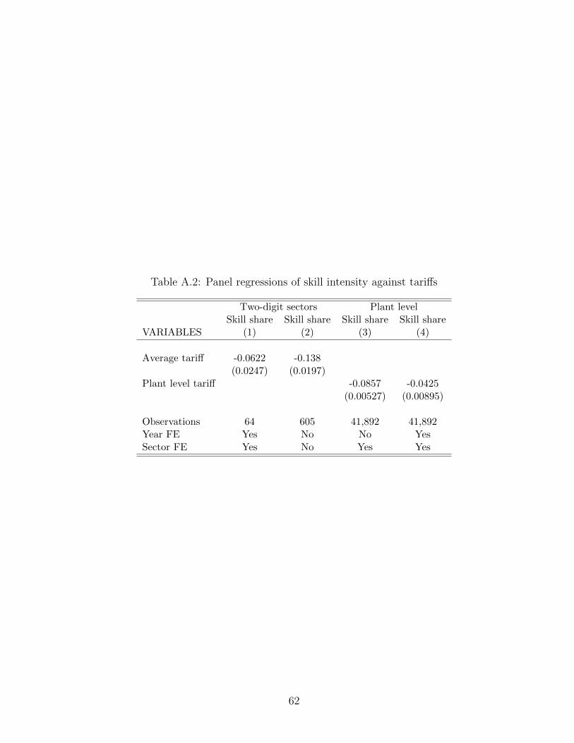
Table A.2: Panel regressions of skill intensity against tariffs
Two-digit sectors Plant levelSkill share Skill share Skill share Skill share
VARIABLES (1) (2) (3) (4)
Average tariff -0.0622 -0.138(0.0247) (0.0197)
Plant level tariff -0.0857 -0.0425(0.00527) (0.00895)
Observations 64 605 41,892 41,892Year FE Yes No No YesSector FE Yes No Yes Yes
62

Table A.3: Cross-sectional Patterns across Sectors
sector skill intensity exporting firms importing firmsq1 q2 q3 q4 q1 q2 q3 q4 q1 q2 q3 q4
311 0.30 0.29 0.33 0.40 1% 2% 3% 15% 3% 11% 16% 44%313 0.37 0.46 0.57 0.37 0% 0% 3% 6% 28% 21% 33% 82%314 0.21 0.18 0.46 0.42 0% 0% 67% 33% 0% 33% 67% 67%321 0.28 0.31 0.30 0.26 3% 4% 8% 39% 1% 5% 13% 58%322 0.18 0.21 0.20 0.26 7% 3% 4% 19% 1% 0% 0% 7%323 0.17 0.20 0.23 0.24 9% 29% 35% 83% 4% 21% 22% 58%324 0.18 0.21 0.17 0.22 4% 3% 7% 32% 0% 0% 5% 23%331 0.19 0.19 0.21 0.25 2% 2% 2% 15% 2% 2% 9% 32%332 0.19 0.20 0.21 0.29 6% 2% 6% 4% 2% 2% 4% 17%341 0.24 0.22 0.34 0.38 0% 3% 14% 30% 3% 14% 25% 49%342 0.24 0.30 0.33 0.42 1% 1% 3% 27% 8% 10% 18% 47%351 0.34 0.40 0.45 0.45 3% 15% 25% 76% 19% 42% 53% 91%352 0.41 0.45 0.49 0.57 3% 5% 21% 58% 27% 47% 78% 96%355 0.31 0.24 0.30 0.28 0% 10% 5% 55% 15% 35% 60% 80%356 0.18 0.28 0.29 0.30 1% 2% 15% 33% 3% 13% 42% 64%361 0.08 0.15 0.28 0.21 0% 0% 14% 100% 29% 14% 43% 100%362 0.26 0.29 0.30 0.29 6% 0% 18% 56% 24% 17% 59% 78%369 0.19 0.21 0.19 0.27 0% 1% 1% 16% 3% 5% 8% 27%371 0.24 0.16 0.25 0.37 0% 0% 12% 18% 0% 24% 41% 76%372 0.24 0.34 0.40 0.34 13% 0% 25% 25% 13% 25% 88% 88%381 0.25 0.26 0.29 0.30 1% 1% 8% 35% 13% 15% 29% 65%382 0.21 0.27 0.28 0.34 6% 14% 15% 35% 16% 29% 38% 78%383 0.31 0.32 0.36 0.40 0% 2% 17% 41% 26% 34% 66% 93%384 0.28 0.24 0.29 0.34 2% 5% 10% 30% 12% 28% 42% 80%385 0.35 0.34 0.35 0.34 11% 11% 22% 47% 28% 28% 50% 68%390 0.23 0.24 0.22 0.36 5% 7% 19% 58% 17% 14% 36% 81%all 0.23 0.25 0.29 0.36 3% 4% 9% 30% 6% 11% 23% 57%
63
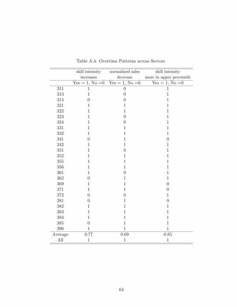
Table A.4: Overtime Patterns across Sectors
skill intensity normalized sales skill intensity
increases decrease more in upper percentile
Yes = 1, No =0 Yes = 1, No =0 Yes = 1, No =0311 1 0 1313 1 0 1314 0 0 1321 1 1 1322 1 1 1323 1 0 1324 1 0 1331 1 1 1332 1 1 1341 0 1 0342 1 1 1351 1 0 1352 1 1 1355 1 1 1356 1 1 1361 1 0 1362 0 1 1369 1 1 0371 1 1 0372 0 0 1381 0 1 0382 1 1 1383 1 1 1384 1 1 1385 0 1 1390 1 1 1
Average 0.77 0.69 0.85All 1 1 1
64

Table A.5: Correlation between price-adjusted sales q and other firm characteristics
white-collar shares 0.110(0.000)
log of average firm wage 0.260(0.000)
input price 0.140(0.000)
output price 0.554(0.000)
import status 0.118(0.000)
import share 0.084(0.000)
export status 0.165(0.000)
export share 0.105(0.000)
log of sales 0.319(0.000)
log of domestic sales 0.311(0.000)
The table shows the correlations between price-adjusted sales q and the listed firm characteristics. P-values in parentheses.
65

B Theory appendix
Appendix B.1 develops intuition behind function Φ in the production function. Appendix B.2
illustrates firms’ quality choices. Appendix B.3 proves the claim in section 3.1 that firms only
increase quality if their sales increase.
B.1 Theory: Function Φ
This appendix develops further intuition for function Φ. In the production function (1), Φ(q′, q)
is a productivity shifter associated with input quality q′ in the production of a good with quality
q. Section 3 assumes
Φ(q′, q) = φ(q′)
[exp(q′ − νq)
1 + exp(q′ − νq)
]where ν ≥ 0 is a parameter. A firm with output quality q has the following relative demand for
any two material inputs 1 and 2:
x(1)
x(2)=
(p1
p2
)−σ Φ(q1, q)
Φ(q2, q).
A well known result is that if q1 > q2, then Φ(q1,q)Φ(q2,q)
is increasing in q if and only if function Φ is
log-supermodular—i.e., if the cross-partial derivative of log(Φ) is positive:
∂2 log(Φ(q′, q))
∂q′∂q=
ν exp(q′ − νq)[exp(q′ − νq) + 1]2
which holds if ν > 0.
To further intuition, let φ(q′) = 1. This term governs only prices in the estimation and has
no effect on relative demand. Figure B.1 plots the relative term[
exp(q′−νq)1+exp(q′−νq)
]as a function
of input quality q′ for a specific output quality q. The function is the cumulative distribution
function of a logistic random variable with νq as the inflection point. If input prices rise slowly
with quality, the firm with output quality q concentrates its input purchases around the oval.
Inputs of quality q′ < νq are very inefficient in producing quality q, and inputs with quality
much higher than νq may be more expensive or not available. If ν > 1 as estimated (ν = 1.1)
66
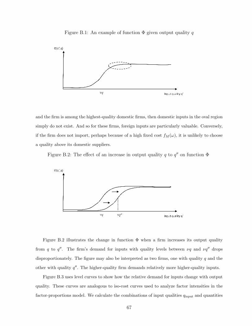
Figure B.1: An example of function Φ given output quality q
and the firm is among the highest-quality domestic firms, then domestic inputs in the oval region
simply do not exist. And so for these firms, foreign inputs are particularly valuable. Conversely,
if the firm does not import, perhaps because of a high fixed cost fM (ω), it is unlikely to choose
a quality above its domestic suppliers.
Figure B.2: The effect of an increase in output quality q to q′′ on function Φ
Figure B.2 illustrates the change in function Φ when a firm increases its output quality
from q to q′′. The firm’s demand for inputs with quality levels between νq and νq′′ drops
disproportionately. The figure may also be interpreted as two firms, one with quality q and the
other with quality q′′. The higher-quality firm demands relatively more higher-quality inputs.
Figure B.3 uses level curves to show how the relative demand for inputs change with output
quality. These curves are analogous to iso-cost curves used to analyze factor intensities in the
factor-proportions model. We calculate the combinations of input qualities qinput and quantities
67

xinput that deliver the same output—i.e., the same value for
x(σ−1)/σinput
[exp(qinput − qoutput)
1 + exp(qinput − qoutput)
]
in equation (3), where we pick ν = 1. We repeat this exercise for three levels of output quality
qoutput = 1, 2, 3 and pick the level curves to cross at where the quality and quantity of input
are one xinput = qinput = 1. The gradient of the level curve is clearly flatter for the solid line,
corresponding to the higher-quality output. This result implies that higher-quality firms are
intensive in higher-quality inputs: When output quality is high, a larger quantity of inputs is
needed to compensate for any decrease in input quality. All three curves become flat as the
quality of the input increases much beyond the output quality. This result arises because Φ
tends to one as the quality of the input tends to infinity, and so no increase in input quality
compensates for a sufficiently large drop in quantity.
Figure B.3: Combinations of inputs quality and quantities that deliver the same output
Simulations of the model in section 4 reduce firms’ quality choices to a grid of 200 quality
levels in [0, 10]. This upper bound in function Φ is convenient to maintain quality choices in the
grid, but an alternative specification of function Φ in appendix D shows that an upper bound is
not crucial.58 More crucial to maintain quality choices within the grid is that function Φ tends
to zero in its lower tail, if the difference between input and output quality (qinput − νqoutput)
58If the input cost did not change with quality, this upper bound limq′→∞Φ(q′, q) = 1 would implythat the revenue gain from upgrading quality is zero when z2(ω) = 0 in equation (17), but for firms thathave a comparative advantage in producing higher-quality the revenue gain would not tend to zero.
68

goes to minus infinity. This property implies that if a firm increases its output quality much
beyond available inputs, its material input costs C(q) go to infinity.
B.2 Theory: Quality choices
This appendix illustrates a firm’s quality choices, and the effects of international trade and
productivity on this choice. Consider a firm with productivity z(q) = 1 and three of its choices
on international trade: (1) not import or export, (2) to import only and (3) to import and
export. This choice of z is close to the average in the estimated model, 1.1. We disregard
the possibility of only exporting because very few firms export and not import in the estimated
model and data. Using the cost and revenue functions in the main text and the profit in equation
(12), its profit under the three discrete choices is
π1(q) = σP (q, 0)−(1−α)(σ−1)χ(q)− f(q)
π2(q) = σP (q, 1)−(1−α)(σ−1)χ(q)− f(q)− fM
π3(q) = σP (q, 1)−(1−α)(σ−1)(χ(q) + χ∗(q))− f(q)− fM − fX
where σ = σ−σ(σ − 1)σ−1 is a constant and χ∗(q) = Φ(q,Q∗)Y ∗ following foreign demand in
equation (7). We have simplified the notation by dropping firm index in fixed costs fX and fM .
Figure B.4(a) graphs operating profits of the three cases using the price indices P and
demand functions χ, χ∗ from the estimated model. Operating profits are initially increasing in
q, it reaches a maximum around q = 3 or 4, depending on participation in international trade,
and declines thereafter. Initial increase is due to an increase in sales χ associated with higher
quality, and the eventual decline is due to the cost of material inputs, P (q, 1M ), that increases
because the production of higher quality uses higher-quality inputs.
Figure B.4(b) illustrates the first order conditions. The schedules are the derivatives of
operating profits in figure B.4(a). The horizontal line is the derivative of fixed costs f ′(q) = f2.
It is close to the x-axis because estimated f2 = 5 × 10⁻⁵ ≈ 0. The firm chooses quality in the
intersection of the derivative of operating profits with f ′(q). It chooses q = 2.7 if it remains
domestically-oriented, q = 2.9 if it imports only, and q = 3.6 if it imports and export. In words,
69
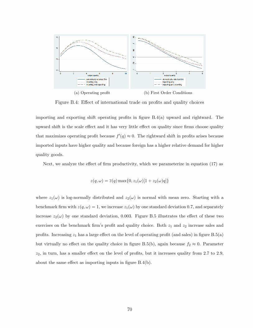
(a) Operating profit (b) First Order Conditions
Figure B.4: Effect of international trade on profits and quality choices
importing and exporting shift operating profits in figure B.4(a) upward and rightward. The
upward shift is the scale effect and it has very little effect on quality since firms choose quality
that maximizes operating profit because f ′(q) ≈ 0. The rightward shift in profits arises because
imported inputs have higher quality and because foreign has a higher relative demand for higher
quality goods.
Next, we analyze the effect of firm productivity, which we parameterize in equation (17) as
z(q, ω) = z(q) max0, z1(ω)[1 + z2(ω)q]
where z1(ω) is log-normally distributed and z2(ω) is normal with mean zero. Starting with a
benchmark firm with z(q, ω) = 1, we increase z1(ω) by one standard deviation 0.7, and separately
increase z2(ω) by one standard deviation, 0.003. Figure B.5 illustrates the effect of these two
exercises on the benchmark firm’s profit and quality choice. Both z1 and z2 increase sales and
profits. Increasing z1 has a large effect on the level of operating profit (and sales) in figure B.5(a)
but virtually no effect on the quality choice in figure B.5(b), again because f2 ≈ 0. Parameter
z2, in turn, has a smaller effect on the level of profits, but it increases quality from 2.7 to 2.9,
about the same effect as importing inputs in figure B.4(b).
70

(a) Operating profit (b) First Order Conditions
Figure B.5: Effect of productivity parameters z1, z2 on profits and quality choices
B.3 Theory with ν = 0
Section 3.1 describes the model with ν = 0. This section shows that firms never upgrade when
(i) sales do not increase, (ii) the skill premium increases and (iii) higher-quality production is
skill intensive. Intuitively, points (ii) and (iii) together imply that the cost of producing higher
quality increases and so sales must strictly increase for quality upgrading to become profitable.
We provide two proofs. The first is simpler and assumes all functions are differentiable. The
proof without differentiability is general enough to include the case where labor is elastic and
wages do not change.
Proof with differentiability. From section 3.1, we only need to prove that εpq increases in
the skill premium. Taking derivatives of the price in equation (15) when ν = 0, we have
εpq =dp(q, ω)
dq
q
p(q, ω)= q
[αw′(q)
w(q)− zq(q, ω)
z(q, ω)
]= q
α
1− σL
[(ws/wu)1−σLΦLq(s, q) + ΦLq(u, q)
(ws/wu)1−σLΦL(s, q) + ΦL(u, q)
]− zq(q, ω)
z(q, ω)
where ΦLq denotes the derivative of ΦL with respect to the first argument. The third line factors
out w1−σLu from the numerator and denominator and uses the definition of w(q) in equation (10):
w(q) =
[∑ς=u,s
w(1−σL)ς ΦL(ς, q)
]1/(1−σL)
.
71

Taking derivatives of εpq above with respect to the skill premium (ws/wu), we get:
∂εpq∂(ws/wu)
= αq(ws/wu)−σL
w(q)2(1−σL)[ΦLq(s, q)ΦL(u, q)− ΦLq(u, q)ΦL(s, q)] (B.1)
By definition, higher-quality production is more skill intensive if ΦL(s,q)ΦL(u,q) is increasing in quality
q. The derivative
d
dq
[ΦL(s, q)
ΦL(u, q)
]=
ΦLq(s, q)ΦL(u, q)− ΦLq(u, q)ΦL(s, q)
ΦL(u, q)2
has the same sign as equation (B.1). Then, εpq increases with the skill premium.
Proof without differentiability. Denote the periods before and after the trade liberalization
with superscripts N and T respectively. The contradiction hypothesis is that a firm chooses
quality qA in period T and qB in period N such that qA > qB and
πT (qA) ≤ πN (qB)
where π are operating profits and the inequality holds because revenue equals operating profit
times σ. Because the firm chooses qB before the trade liberalization and qA afterward
πN (qA)− f(qA) ≤ πN (qB)− f(qB)
πT (qB)− f(qB) ≤ πT (qA)− f(qA)
Since the fixed cost does not change, summing the inequalities above yield
πN (qA)− πN (qB) ≤ πT (qA)− πT (qB)
≡ πN (qB)
(πN (qA)
πN (qB)− 1
)≤ πT (qB)
(πT (qA)
πT (qB)− 1
)(B.2)
Since upgrading is costly and the firm upgrades at time T , πT (qA) > πT (qB). Together with the
contradiction hypothesis, this implies that πN (qB) > πT (qB). Then, the inequality in equation
72

(B.2) must hold strictly for the term in parenthesis:
πN (qA)
πN (qB)<πT (qA)
πT (qB)
⇔ qAqB
(z(qA, ω)
z(qB, ω)
)σ−1(wN (qA)
wN (qB)
)α(1−σ)
<qAqB
(z(qA, ω)
z(qB, ω)
)σ−1(wN (qA)
wN (qB)
)α(1−σ)
⇔ wN (qA)
wN (qB)>wT (qA)
wT (qB)
where the second line simply uses the expressions for operating profits from section 3.1, and
the third line rearranges considering σ > 1. But this contradicts the hypothesis that the skill
premium increased and that higher quality qA is more skill intensive. To see this, we substitute
the expression for the wage index:
w(qA)
w(qB)=φL(u, qA)
11−σ
φL(u, qB)1
1−σ
(wswu
)1−σΦL(s,qA)ΦL(u,qA) + 1(
wswu
)1−σΦL(s,qB)ΦL(u,qB) + 1
1
1−σ
Taking derivatives with respect to wages, it is straightforward that the ratio w(qA)w(qB) increases in
the skill premium if and only if ΦL(s,qA)ΦL(u,qA) >
ΦL(s,qB)ΦL(u,qB)—i.e., quality A is more skill intensive.59
C Quantitative analysis
We present supplementary material for estimation and counterfactuals. Appendix C.1 discusses
computational issues. Appendix C.2 discusses the parametrization of all skill-related variables.
The procedure to estimate standard errors is in appendix C.3. Appendix C.4 presents a back-
of-the-envelope calculation to compare the magnitudes of changes in demand for skills in the
counterfactuals with elastic and inelastic labor. Appendix C.5 estimates the model with ν = 0.
Appendix C.6 explains why percentile shifts in skill intensity were smaller than the aggregate
increase in skill intensity in counterfactuals (table 13). Appendix C.7 details moments from the
estimation and counterfactuals not present in the main text.
59To take derivatives, it is easier to transform the problem and show that xa+1xb+1 is increasing in x if and
only if a > b.
73
C.1 Computational issues
Parameters Γ1 = ν, µ1, σ1, σ2, f1, f2, µM , µX , σM , σX , Y∗, Q∗, q∗ govern quality, sales, import
and export choices. These choices are intertwined in the model—within and across firms. With
the normalization w(q) = 1 and [z(q)]σ−1φ(q) = 1, parameters Γ2 = λ1, λ2, ws, εL, z3 map
quality choices to unit prices and skills, but they do not enter the firm’s problem (12). This
assumption greatly facilitates computation and the identification of parameters. We use a sim-
plex and a simulated annealing algorithm to estimate the model. These algorithms iterate over
13 parameters Γ1 that jointly determine the following moments:
• 10%, 25%, 50%, 75%, 90% of the unconditional distribution of sales (5)
• By quartile of domestic sales, share of plants importing, share of plants exporting, average
spending on imported inputs/total spending on materials, average export sales/total sales
(16)
• share of firms in the nth quartile of domestic sales and the mth quartile (16)
• exit rate (1)
These moments do not depend on parameters Γ2 when w(q) = 1 and [z(q)]σ−1φ(q) = 1. So,
for each guess of the 13 parameters above, we run an inner optimization algorithm that picks
Γ2 to best match the remaining moments:
• 10%, 25%, 50%, 75%, 90% of the unconditional distribution of white-collar shares (5)
• average wage of white collars/average wage of blue collars (1)
• aggregate share white collars/average wage of blue collars (1)
• coefficient of the regression of output prices on measured skill intensity (1)
• coefficient of the regression of input prices on measured skill intensity (1)
Since there is no firm choice in this inner stage, the inner optimization algorithm takes less
than one second to run for a typical guess of Γ1. This method works much better and moments
are much more stable than if we allowed parameters Γ2 to change quality choices, and together
change all moments on sales, import and export behavior that do not help in their identification.
74

C.1.1 Melitz (2003) and aggregate functions P , χ
From section 4.2, functions P and χ are calculated for each parameter guess, and for each guess
of firms’ discrete choices exit, quality q, import and export status. The aggregation of firms
into a representative firm in Melitz (2003) significantly speeds up the computation of these two
functions. Price indices are defined in equation (8):
P (q) =
[∫Ωp(ω)1−σΦ(q(ω), q)dω
]1/(1−σ)
(C.1)
P ∗(q) =
[∫Ω∗p(ω)1−σΦ(q(ω), q)dω
]1/(1−σ)
P (q, 1M ) =[P (q)1−σ + 1MP
∗(q)1−σ]1/(1−σ)(C.2)
where the price of firm ω is itself a function of price indices:
p(ω) = µP (q, 1M )1−α
z(q, ω)(C.3)
since w(q) = 1 in the estimation. For each guess of parameters, Foreign price P ∗(q) is given
since it depends only on p∗ = 1, q∗, ν and the measure of Foreign firms set to 1. One way of
computing prices P (q) and P (q, 1) is to iterate over the 100,000 firms in the simulation. That
is, given an initial guess of P (q), we can calculate P (q, 1) from equation (C.2) and individual
firms’ prices from equation (C.3). Plugging these firm prices back into the right-hand-side of
equation (C.1) gives us a new guess of P (q). This approach works but it is inefficient.
Instead of iterating over all 100,000 firms, we can define a representative firm for each quality
level and each import status 1M , and iterate over these representative firms. Let Ω(q, 1M ) be
the set of firms with quality q and m(q, 1M ) = |Ω(q, 1M )| be the mass of firms with quality q and
import status 1M .60 Then, following Melitz (2003), the productivity of a representative firm as
zR(q, 1M ) =
[1
m(q, 1M )
∫ω∈Ω(q,1M )
z(ω, q)σ−1dω
] 1σ−1
.
Importantly, this productivity and masses m(q, 1M ) do not depend on functions P and χ, only
60Each firm has a mass of 1/100,000.
75
on the guesses of parameter and on discrete choices of firms. So, they may be calculated before
the estimation of P and χ.
Given a guess of P (q), we calculate P (q, 1) from equation (C.2) and the price of this repre-
sentative firm as
pR(q, 1M ) = µP (q, 1M )1−α
zR(q, 1M )(C.4)
The aggregate price index as a function of these representative firms is
P (q) =
∑q′,1M
m(q′, 1M )pR(q′, 1M )1−σΦ(q′, q)
1/(1−σ)
(C.5)
So, we can simply iterate over the last two equations. In the simulations, the quality grid has
200 choices. Together with 1M ∈ 0, 1, this gives us at most 400 discrete choices, most of which
do not have any firms for a typical guess of parameters and firm choices. So, iterating over these
representative firms in equations (C.4) and (C.5) is much quicker than iterating over equations
(C.1) and (C.3). The optimization algorithm uses the later iteration. With a small probability,
it checks that the computed fixed point of equation (C.5) is the same as equation (C.1).
The estimation of function χ follows a similar strategy and we only sketch it here. The
reader may turn to the programs for details. Function χ is a fixed point of equation (11),
χ(q) = Φ(q, 0)P (0, 1)σ−1Y +1− αµ
∫Ω
Φ(q, q(ω))P (q(ω), 1M (ω))σ−1rT (ω)dω.
It is a fixed point because a firm’s spending on materials 1−αµ rT (ω) is itself a function of demand
χ. The only difference in calculating χ relative to price indices P is that the demand for materials
is a function of firms’ export status. And so, we need a representative firm for each choice of
quality q import and export statuses 1M and 1X to get the price of this representative firm and
its demand rT . Since the price indices do not depend on χ, they are calculated before and used
in the estimation of function χ.
76
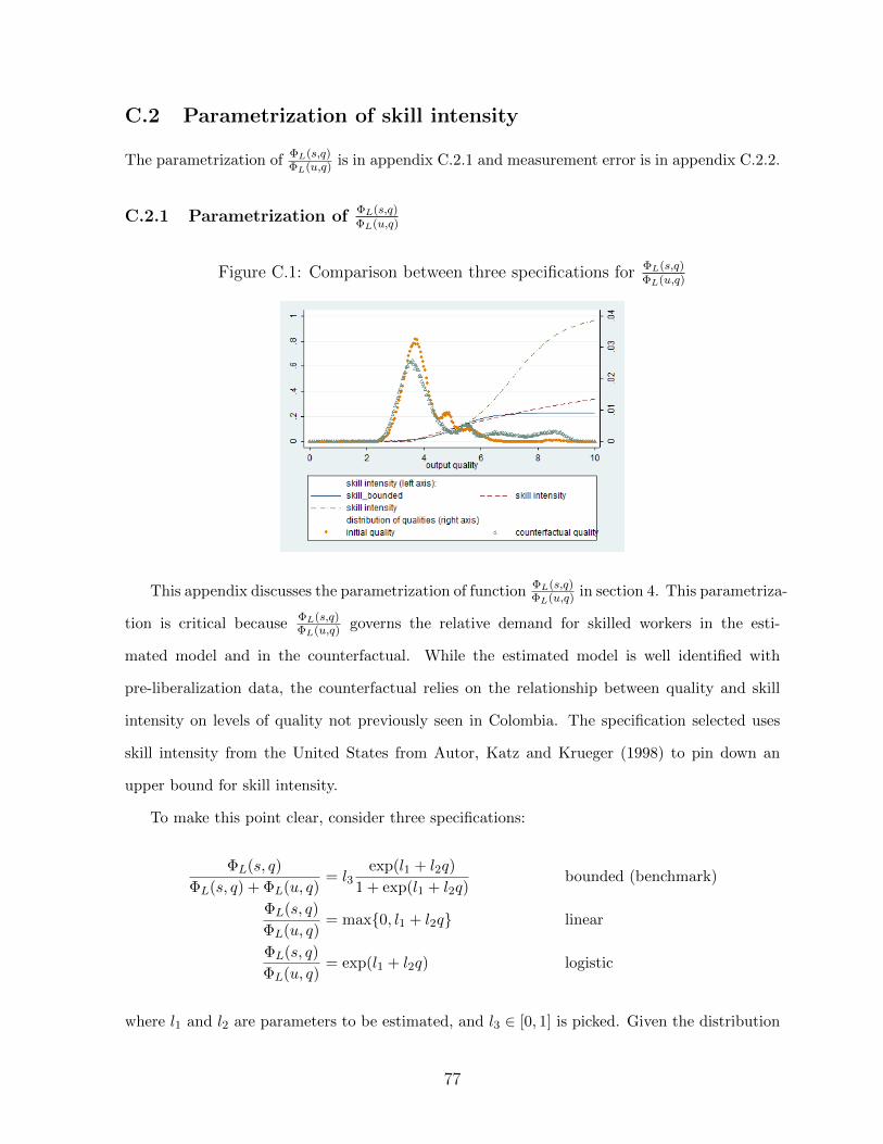
C.2 Parametrization of skill intensity
The parametrization of ΦL(s,q)ΦL(u,q) is in appendix C.2.1 and measurement error is in appendix C.2.2.
C.2.1 Parametrization of ΦL(s,q)ΦL(u,q)
Figure C.1: Comparison between three specifications for ΦL(s,q)ΦL(u,q)
This appendix discusses the parametrization of function ΦL(s,q)ΦL(u,q) in section 4. This parametriza-
tion is critical because ΦL(s,q)ΦL(u,q) governs the relative demand for skilled workers in the esti-
mated model and in the counterfactual. While the estimated model is well identified with
pre-liberalization data, the counterfactual relies on the relationship between quality and skill
intensity on levels of quality not previously seen in Colombia. The specification selected uses
skill intensity from the United States from Autor, Katz and Krueger (1998) to pin down an
upper bound for skill intensity.
To make this point clear, consider three specifications:
ΦL(s, q)
ΦL(s, q) + ΦL(u, q)= l3
exp(l1 + l2q)
1 + exp(l1 + l2q)bounded (benchmark)
ΦL(s, q)
ΦL(u, q)= max0, l1 + l2q linear
ΦL(s, q)
ΦL(u, q)= exp(l1 + l2q) logistic
where l1 and l2 are parameters to be estimated, and l3 ∈ [0, 1] is picked. Given the distribution
77

of quality in the estimated model, we estimate parameters l1 and l2, under the logistic and linear
specifications above, using all moments related to skill intensity and wages. The relationships
between skill intensity and quality from this exercise are on the left axis of figure C.1. On the
right y-axis is the distribution of quality from the estimated model (solid circles) and from the
counterfactual trade liberalization with elastic labor of section 6 (hollow triangles). Since wages
are maintained at w(q) = 1 when labor is elastically supplied the counterfactual distribution
does not depend on function ΦL(s,q)ΦL(u,q)—see appendix C.1 above.
The predictions of the model under the three skill specifications are similar for the estimated
quality choices but they differ in the counterfactual qualities. For example, the 90th percentile
of the distribution of quality is q = 5.1 in the estimated model and q = 6.8 in the counterfactual.
When q = 5.1, skill intensity is about 11% in all three specifications. When q = 6.8, skill intensity
is 22% in the bounded and linear specifications, and it is 43% in the logistic specification. So the
logistic specification delivers much larger counterfactual changes in skill intensity. The linear
specification, in turn, does not capture the cross section as well since it predicts 0 skill intensity
for many firms. We use the bounded specification because it makes more conservative and
realistic counterfactual predictions.
C.2.2 Measurement error εL
Measurement error in labor εL is critical for the model to match moments related to skills, and
for the comparison of our results to AGP. Parameters λ1, λ2, ws, εL map these quality choices
to skill-related moments. To illustrate the role of measurement error, we re-estimate parameters
λ1, λ2, ws setting εL = 0. When εL = 0, measured and actual skill intensity are the same.
To give the model a chance to match data, we drop the upper limit on the skill distribution
because aggregate white-collar shares in the data is 29% and skill intensity in the USA was 23%
in the 1980s. That is, we set λ3 = 1. As shown above in appendix C.2.1, λ3 is not important in
matching moments in the estimation—it is important only for the counterfactual results. Tables
C.1 through C.3 compare the results of the model estimated in the main text with measurement
error (labeled “general model”) with the model without measurement error εL = 0.
Within sample, the model with εL = 0 grossly underestimates the spread in the distribution
78

Table C.1: Unconditional distribution of sales and measured skill intensity
10th 25th 50th 75th 90th
white-collar shares, in %data 5.9 13 22 34 50general model 6.2 12 21 34 49εL = 0 15 18 20 24 31
Table C.2: Joint distributions of sales with other characteristics (in %)
quartiles of domestic sales1 2 3 4 (largest)
share of white-collar workersdata 20 22 26 34general model 22 24 26 29εL = 0 18 20 23 28
Table C.3: Aggregate skill intensity and premium
measured skill (targeted) data general model εL = 0skill intensity Lwhite/L (in %) 29 32 32skill premium wwhite/wblue 1.59 1.59 1.59
unobserved skill (out of sample) Colombian avg.† model εL = 0skill intensity Ls/L (in %) 8.5 11.6 32skill premium ws/wu 1.8 - 2.6 2.8 1.59† The Colombian average is from Attanasio, Goldberg, Pavcnik (2004).
of skill intensity on table C.1. The reason is as follows. Since most large firms have high average
wages in figure 2, the model with ε = 0 predicts that skill intensity in the 90th percentile is very
close to the aggregate skill intensity on table C.3. Similarly, it predicts that the 10th percentile
is close to skill intensity in the lowest quartile of wages on table C.2.
Out of sample, the model with ε = 0 precludes the comparison of our results to AGP.
Aggregate white collar shares in the data and model are about 30%, which is much higher than
the share of college graduates in Colombia at the time, on table C.3.
Mechanically, the main text states that the share of unskilled workers misclassified as white-
collar workers is independently drawn for each firm from a logistic distribution truncated in
[0, ls/l] with mean parameter zero and variance parameter εL. That is, consider a firm in the
model with ls skilled workers and lu = (l− ls) unskilled workers. We draw its measurement error
79

term ε from a distribution with cumulative distribution function (cdf) Ftrunc(ε) = F (ε)F (ls/lu) where
F is the corresponding unconditional cdf F (ε′) = exp(ε′/εL)exp(ε′/εL)+1 . The firm has ls + luε white-collar
workers and lu(1− ε) blue-collar workers.
C.3 Standard errors
This appendix details the procedure to estimate standard errors. See Dix-Carneiro (2014) web
appendix I for proof. Let p be the number of parameters and m the number of moments. The
vector of parameter estimates Θ is:
Θ = arg minΘ
(δ − δS(Θ))′W (δ − δS(Θ))
where W is the symmetric positive definite m ×m matrix of weights, δ is a vector of observed
moments and δS(Θ) is the corresponding vector of simulated moments when the vector of pa-
rameters is Θ. Let ∇g be the m× p matrix of derivatives of δS(Θ) with respect to Θ, estimated
numerically. We estimate the variance of data moments V through bootstrap by randomly
drawing firms with replacement and recalculating moments. Under the estimating null that the
model is correctly specified, estimated Θ converges to the true Θ0. Thus the variance of the
simulated moments is simply 1SV , where S is the number of simulations. Then, the estimated
variance of parameters is
Var(Θ−Θ0) =(∇g′W∇g
)−1∇g′W [V (1 +1
S)]W∇g
(∇g′W∇g
)−1
Benchmark estimates take W to be the identity matrix. Appendix D.2 estimates it using
the inverse of the variance W = V −1 which reduces the formula to
Var(Θ−Θ0) = (1 +1
S)(∇g′W∇g
)−1.
80

C.4 Back-of-envelope comparison of elastic and inelastic coun-
terfactuals
To compare the magnitudes of changes in demand for skilled worker in the elastic and inelastic
counterfactuals, suppose that aggregate demand relative demand for skilled labor took the form:
LstLut
=
(wstwut
)−σLSt (C.6)
where σL is the constant elasticity of substitution between skilled and unskilled workers, St is
a shifter. Denote with t = 0 the model before the trade liberalization and with t = 1. In this
simple framework, the trade liberalization is simply a change in the relative demand for labor
captured by St. In the counterfactual with elastic labor, the skill premium does not change:
ws0wu0
= ws1wu1
. Then, we can use the estimated change in skill intensities to calculate the change in
demand shifters S1S0
:
Ls1Lu1
Lu0
Ls0=S1
S0.
The question in section 6.2 is the change in skill premium w that would have maintained skill
intensity constant in the elastic labor counterfactual if demand took the form of equation (C.6):
1 = (w)−σLS1
S0(C.7)
With elastic labor, the skill intensity rose from 0.116 to 0.161. Substituting Ls1Lu1
= 0.1161−0.116 and
Ls0Lu0
= 0.1611−0.161 , we get w = ws1
wu1wu0ws0
= 1.27.
C.5 Estimation of ν = 0 case
This appendix estimates the model with ν = 0. The only change in the parametrization with
respect to the benchmark is that we allow the fixed cost of production to be convex:
f(q) = f1 + f2qf3 (C.8)
81

where f1 ≥ 0, f2 ≥ 0 and f3 are parameters to be estimated. The fixed cost of production
f(q) = f1 + f2q is linear in the general model where quality choices are naturally constrained by
the lack of availability of high-quality inputs. The added parameter f3 does not improve the fit
of the general model. When ν = 0, firms with positive productivity draws z2(ω) would choose
infinite quality if fixed costs were not sufficiently convex. When ν = 0, the quality of Foreign
inputs is irrelevant and we set q∗ = 0.
Table C.4: Parameter estimates (est) and standard errors (se) for model with ν = 0
α = 0.7 α = 0.5est se est se
µ1 -0.283 0.005 -0.287 0.004σ1 0.492 0.003 0.492 0.003σ2 0.008 0.001 0.006 0.000z3 -0.833 0.054 -0.715 0.039f1 0.001 3.8E-05 0.002 3.6E-05f2 1.9E-10 1.8E-11 2.9E-10 4.6E-11f3 10.8 0.479 9.9 0.124µM -3.607 0.039 -2.933 0.055σM 2.363 0.020 2.464 0.032µX 0.378 0.143 0.382 0.075σX 3.645 0.091 3.642 0.061λ1 -7.318 0.519 -6.892 0.698λ2 1.685 0.188 1.430 0.158ws/wu 2.741 0.025 2.768 0.028Y ∗ 0.314 0.020 0.291 0.020Q∗ 3.120 0.157 3.420 0.140εL 0.151 0.001 0.151 0.002
Table C.4 presents the parameter estimates when α = 0.7 in the benchmark, and when
α = 0.5 in alternative A3 of section 7.1. Changes in the density of the quality distribution for
the counterfactual with elastic labor are in figure C.2. As mentioned in section 6.1, firm quality
barely changes. Other counterfactual results are in main text and in appendix C.7.
C.6 Counterfactual shifts in white-collar shares
This appendix reconciles counterfactual shifts in the distribution of white-collar shares with its
aggregate changes on table 13. Shifts in percentiles are typically smaller than the total. We use
82

Figure C.2: Counterfactual changes in quality when ν = 0, elastic labor
the example with elastic labor to explain how shifts in employment, from the less to the more
skill intensive firms can generate this result.
Table C.5 partitions firms by quartiles of white-collar shares. It reports the share of white-
collar workers and the share of employment in each quartile before and after the counterfactual.
The sum of the product of lines (A) and (B) is the total share of white-collar workers before
the trade liberalization, 32%, and the sum of the product of lines (C) and (D) is the total share
of white-collar workers post-liberalization, 37%. Employment shares in lines (B) and (D) add
to 100%. The last two lines report the difference between pre- and post-liberalization. In line
(E), the increase in white-collar shares is always smaller in the quartiles than in the aggregate
as on table 3. This result is explained with line (F): Employment shares shift from less to more
skill-intensive firms.61
Bustos (2011), Kugler and Verhoogen (2012) and Pavcnik (2002) provide evidence that
ex ante larger firms grow and invest in product and process innovation relative to other firms
following a trade liberalization. Since larger firms are typically more skill intensive, these findings
are consistent with shifts in employment on table 3. But these shifts do not appear in the
Colombian data, possibly because we look at the raw data without controls and interactions
with tariff cuts that these other papers use.
61This result is analogous to the effect of trade on a skill abundant country in a factor-proportionsmodel: The skill intensity decreases in all sectors and the production of skill intensive goods increases.
83
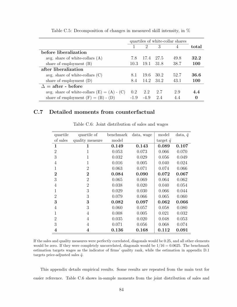
Table C.5: Decomposition of changes in measured skill intensity, in %
quartiles of white-collar shares
1 2 3 4 totalbefore liberalization
avg. share of white-collars (A) 7.8 17.4 27.5 49.8 32.2share of employment (B) 10.3 19.1 31.8 38.7 100
after liberalizationavg. share of white-collars (C) 8.1 19.6 30.2 52.7 36.6share of employment (D) 8.4 14.2 34.2 43.1 100
∆ = after - beforeavg. share of white-collars (E) = (A) - (C) 0.2 2.2 2.7 2.9 4.4share of employment (F) = (B) - (D) -1.9 -4.9 2.4 4.4 0
C.7 Detailed moments from counterfactual
Table C.6: Joint distribution of sales and wages
quartile quartile of benchmark data, wage model data, q
of sales quality measure model target q
1 1 0.149 0.143 0.089 0.1072 1 0.053 0.073 0.066 0.0703 1 0.032 0.029 0.056 0.0494 1 0.016 0.005 0.040 0.0241 2 0.063 0.071 0.074 0.0662 2 0.084 0.090 0.072 0.0673 2 0.065 0.069 0.064 0.0624 2 0.038 0.020 0.040 0.0541 3 0.029 0.030 0.066 0.0442 3 0.079 0.066 0.065 0.0603 3 0.082 0.097 0.062 0.0664 3 0.060 0.057 0.058 0.0801 4 0.008 0.005 0.021 0.0322 4 0.035 0.020 0.048 0.0533 4 0.071 0.056 0.068 0.0744 4 0.136 0.168 0.112 0.091
If the sales and quality measures were perfectly correlated, diagonals would be 0.25, and all other elementswould be zero. If they were completely uncorrelated, diagonals would be 1/16 = 0.0625. The benchmarkestimation targets wages as the indicator of firms’ quality rank, while the estimation in appendix D.1targets price-adjusted sales q.
This appendix details empirical results. Some results are repeated from the main text for
easier reference. Table C.6 shows in-sample moments from the joint distribution of sales and
84
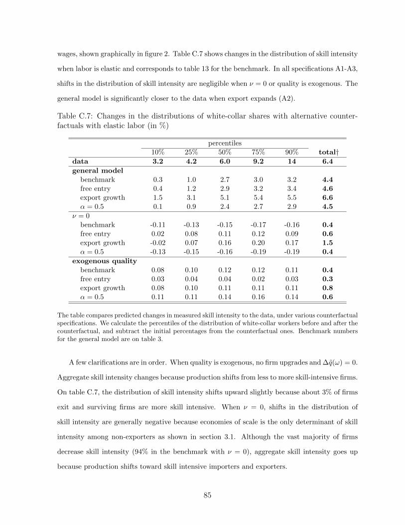
wages, shown graphically in figure 2. Table C.7 shows changes in the distribution of skill intensity
when labor is elastic and corresponds to table 13 for the benchmark. In all specifications A1-A3,
shifts in the distribution of skill intensity are negligible when ν = 0 or quality is exogenous. The
general model is significantly closer to the data when export expands (A2).
Table C.7: Changes in the distributions of white-collar shares with alternative counter-factuals with elastic labor (in %)
percentiles10% 25% 50% 75% 90% total†
data 3.2 4.2 6.0 9.2 14 6.4
general modelbenchmark 0.3 1.0 2.7 3.0 3.2 4.4free entry 0.4 1.2 2.9 3.2 3.4 4.6export growth 1.5 3.1 5.1 5.4 5.5 6.6α = 0.5 0.1 0.9 2.4 2.7 2.9 4.5
ν = 0benchmark -0.11 -0.13 -0.15 -0.17 -0.16 0.4free entry 0.02 0.08 0.11 0.12 0.09 0.6export growth -0.02 0.07 0.16 0.20 0.17 1.5α = 0.5 -0.13 -0.15 -0.16 -0.19 -0.19 0.4
exogenous qualitybenchmark 0.08 0.10 0.12 0.12 0.11 0.4free entry 0.03 0.04 0.04 0.02 0.03 0.3export growth 0.08 0.10 0.11 0.11 0.11 0.8α = 0.5 0.11 0.11 0.14 0.16 0.14 0.6
The table compares predicted changes in measured skill intensity to the data, under various counterfactualspecifications. We calculate the percentiles of the distribution of white-collar workers before and after thecounterfactual, and subtract the initial percentages from the counterfactual ones. Benchmark numbersfor the general model are on table 3.
A few clarifications are in order. When quality is exogenous, no firm upgrades and ∆q(ω) = 0.
Aggregate skill intensity changes because production shifts from less to more skill-intensive firms.
On table C.7, the distribution of skill intensity shifts upward slightly because about 3% of firms
exit and surviving firms are more skill intensive. When ν = 0, shifts in the distribution of
skill intensity are generally negative because economies of scale is the only determinant of skill
intensity among non-exporters as shown in section 3.1. Although the vast majority of firms
decrease skill intensity (94% in the benchmark with ν = 0), aggregate skill intensity goes up
because production shifts toward skill intensive importers and exporters.
85

D Robustness
We present supplementary materials for robustness section 7.2. Appendix D.1 estimates the
model by substituting all moments related to skills in the baseline estimation with price-adjusted
sales q. Appendix D.2 estimates the model with optimal weighting matrix, instead of the
identity matrix used in the baseline estimation. Section D.3 has other specifications. To speed
up computation, when re-estimating the model in this appendix we simulate only 5,000 firms
instead of 100,000 used in the benchmark. Parameter estimates are all on table D.5.
D.1 Robustness: Targeting q
Estimation procedure. We re-estimate the model directly targeting moments on price-
adjusted sales q, which were used only as outside checks on the benchmark model. The estimation
has two stages. In the first stage, we estimate all parameters except for parameters governing
firm’s demand for skills. In a second stage, we estimate skill-related parameters so that we
can compare the predictions of this alternative estimation to the baseline model. Parameters
estimated in the first stage are ν, µ1, σ1, σ2, f1, f2, µM , µX , σM , σX , Y∗, Q∗, q∗, z3 and in the
second stage, they are λ1, λ2, ws, εL, z3. It is worth emphasizing that with this two-stage
approach, all parameters associated with quality choices of inputs and outputs and importing
and exporting are set in the first stage. Counterfactual choices and changes in measured quality
∆q are independent of results in stage two when labor is perfectly elastic and wages remain
w(q) = 1. The counterfactual with inelastic labor depends on skill-related moments. Table D.1
presents the moments targeted in the first and second stages. Other than changing targets, the
remaining estimation procedure and simulations are exactly as in the benchmark.
Estimation results. Table C.6 above shows the joint distribution of sales and price-
adjusted sales q. These quality measures are much less correlated with sales than wages, which
puts an even smaller role for economies of scale in determining quality choices in this estimation.
Tables D.2 and D.3 show the distribution of price-adjusted sales q unconditional and conditional
on domestic sales. These moments were not target in the benchmark and the fit significantly
86

Table D.1: List of moments for estimation targeting q
# of moments
First stage• 10%, 25%, 50%, 75%, 90% of the unconditional distribution of...
... log(normalized domestic sales) 5
... price-adjusted sales q 5• share of firms in the nth quartile of domestic sales and the mth quartile
of q for n,m = 1, ..., 4 16• By quartile of domestic sales, ...
... average price-adjusted sales q 4
... share of plants importing 4
... share of plants exporting 4
... average spending on imported inputs/total spending on materials 4
... average export sales/total sales 4• coefficient of regression of output prices on q 1• coefficient of regression of input unit prices on q 1• yearly exit rate 1total first stage 49
Second stage• 10%, 25%, 50%, 75%, 90% of the unconditional distribution of white-collar shares 5• average white-collar shares by quartile of domestic sales 4• average wage of white collars/average wage of blue collars 1• aggregate share of white-collar workers 1total second stage 11
87
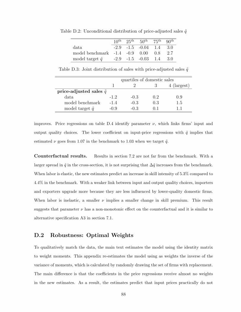
Table D.2: Unconditional distribution of price-adjusted sales q
10th 25th 50th 75th 90th
data -2.9 -1.5 -0.04 1.4 3.0model benchmark -1.4 -0.9 0.00 0.8 2.7model target q -2.9 -1.5 -0.03 1.4 3.0
Table D.3: Joint distribution of sales with price-adjusted sales q
quartiles of domestic sales1 2 3 4 (largest)
price-adjusted sales qdata -1.2 -0.3 0.2 0.9model benchmark -1.4 -0.3 0.3 1.5model target q -0.9 -0.3 0.1 1.1
improves. Price regressions on table D.4 identify parameter ν, which links firms’ input and
output quality choices. The lower coefficient on input-price regressions with q implies that
estimated ν goes from 1.07 in the benchmark to 1.03 when we target q.
Counterfactual results. Results in section 7.2 are not far from the benchmark. With a
larger spread in q in the cross-section, it is not surprising that ∆q increases from the benchmark.
When labor is elastic, the new estimates predict an increase in skill intensity of 5.3% compared to
4.4% in the benchmark. With a weaker link between input and output quality choices, importers
and exporters upgrade more because they are less influenced by lower-quality domestic firms.
When labor is inelastic, a smaller ν implies a smaller change in skill premium. This result
suggests that parameter ν has a non-monotonic effect on the counterfactual and it is similar to
alternative specification A3 in section 7.1.
D.2 Robustness: Optimal Weights
To qualitatively match the data, the main text estimates the model using the identity matrix
to weight moments. This appendix re-estimates the model using as weights the inverse of the
variance of moments, which is calculated by randomly drawing the set of firms with replacement.
The main difference is that the coefficients in the price regressions receive almost no weights
in the new estimates. As a result, the estimates predict that input prices practically do not
88

Tab
leD
.4:
Input
and
outp
ut
pri
ces
A.
Dep
endent
vari
able
:lo
gof
outp
ut
unit
pri
ces
model
dat
ab
ench
mar
kta
rgetq
opti
mal
wei
ghts
whit
e-co
llar
shar
es0.
360.
360.
760.
38(0
.04)
(0.0
1)(0
.05)
(0.0
4)q
0.20
0.12
0.18
0.13
(0.0
02)
(0.0
01)
(0.0
03)
(0.0
02)
B.
Dep
endent
vari
able
:lo
gof
input
unit
pri
ces
model
dat
ab
ench
mar
kta
rgetq
opti
mal
wei
ghts
whit
e-co
llar
shar
es0.
160.
160.
130.
0095
(0.0
2)(0
.002
)(0
.01)
(0.0
06)
q0.
028
0.05
20.
028
0.00
31(0
.001
)(0
.000
1)(0
.000
5)6e
-6
Sta
nd
ard
erro
rsar
ein
par
enth
esis
.A
llco
effici
ents
are
stati
stic
all
ysi
gn
ifica
nt
at
a95%
leve
l.D
ata
regre
ssio
ns
hav
efi
xed
effec
tsfo
rth
eyea
r,th
ep
rod
uct
and
the
sect
orof
the
purc
has
ing
firm
.†I
np
ut
pri
ces
inth
em
od
elin
clu
de
only
dom
esti
cin
pu
tsb
ecau
sew
eca
nn
ot
dis
tin
gu
ish
bet
wee
nF
ore
ign
pri
cesp∗
and
vari
ety|Ω∗ |
.S
imil
arre
gres
sion
sap
pea
rin
Ku
gle
ran
dV
erh
oogen
(2012).
Th
ees
tim
ati
on
targ
ets
the
coeffi
cien
tsof
regre
ssio
ns
wh
enth
ein
dep
enden
tva
riab
leis
wh
ite-
coll
arsh
ares
inth
eb
ench
mark
an
dw
hen
the
ind
epen
den
tva
riab
leisq
inth
ees
tim
ati
on
of
ap
pen
dix
D.1
.T
he
esti
mat
ion
wit
hop
tim
alw
eigh
tsis
inap
pen
dix
D.2
.
89
increase with skill intensity or q (see table D.4)—indicating a lower degree of complementarity
between input and output quality choices. Parameter ν controlling the log-supermodularity in
the demand for inputs decreases from 1.1 to 0.9.
The fit of the model is better in the benchmark relative optimal weights in virtually all
moments—except for the lower tail of the unconditional distribution of firm sales on table 7.
Parameter estimates on table D.5 imply that Foreign relative demand and supply of higher
quality goods is still greater than Home’s (maximum domestic quality is now 6.5). Main coun-
terfactual results are in section 7.2. Changing weights in the estimation with ν = 0 does not
change the results because its estimation ignores input prices by assumption and the coefficient
on output price regressions can always be exactly matched with parameter z3.
D.3 Robustness: Other specifications
We present the remaining robustness checks. The elasticity of substitution between skilled and
unskilled workers σL = 1.6, from Acemoglu and Autor (2010), is estimated using aggregate data
within a year. Since the aggregate elasticity is close to σL in when quality is exogenous, the
choice is adequate if firms do not change quality in the short term (one year). Otherwise, it
should be much smaller. Parameter σL does not affect the elastic-labor counterfactuals where
w(q) = 1. For the inelastic case, we experiment with σ = 1.1 and 1.8, the range of estimates in
the literature.62
The elasticity of substitution between goods σ matters quantitatively and it is unclear what
the optimal parametrization should be. Benchmark σ = 5 is close to the mean estimate using
3-digit product categories in Broda and Weinstein (2006), who estimate the elasticity of sub-
stitution between varieties across countries. We use data from all manufacturing, which should
imply a lower σ. But varieties from different countries may be less substitutable than within
countries, suggesting a higher σ.
Function Φ in equation (5) takes the shape of the cumulative distribution function of a
logistic random variable. It is bounded and has three key properties: It is increasing in input
62These estimates are from Lee, Wolpin (2006) and Katz and Murphy (1992) who use methods similarto Acemoglu and Autor (2010).
90

quality, decreasing in output quality, and log-supermodular. We present here two alternative
functions Φ1 and Φ2:
Φ1(q′, q) = φ(q′)
[exp(ν(q′ − q))
1 + exp(ν(q′ − q)
]and
Φ2(q′, q) = φ(q′)×
exp(q′−q)
1+exp(q′−q) if q′ < q
b(q′ − q + a)ν otherwise
(D.1)
where a = 2ν and b = 1/(2aν) are constants to make Φ continuously differentiable at q′ = q.
Function Φ1 has similar shape from the original. Alternative Φ2 has the key properties above,
but it is not bounded. When q′ < q, it has the same shape as before with ν = 1, which is
between the benchmark ν = 1.1 and ν = 0.9 in appendix D.2.
E Monte Carlo simulations
We perform several simulation exercises. All exercises are suggestive, but combined, they reas-
sure us of the robustness of our empirical exercises. We first verify that results do not change
at all if we double the number of quality choices q ∈ [0, 10] from 200 to 400, or if we expand
the choice set beyond the upper bound of q = 10. On the issue of uniqueness, we do three
exercises: The first is a direct search for multiple equilibria given the parameter estimates. The
second checks whether there are alternative sets of parameters that generate the same moments
as the parameter estimates. This second check addresses uniqueness, identification strategy, and
whether parameter values are robust with respect to changes in the random draws of the 100,000
simulated firms. Third, we check that during counterfactual simulations the economy does not
“jump” to a new equilibrium path.
First, we search for multiple equilibria given the parameter estimates. Starting with random
initial values of firm choices q(ω), 1E(ω), 1M (ω), 1X(ω)ω∈Ω, we search for an equilibrium 1000
times, and in all attempts, we converge to the same exact set of firm choices. That is, none of the
100,000 firms changes its choice even though the initial guesses of q(ω), 1E(ω), 1M (ω), 1X(ω)ω∈Ω
were uniformly distributed over the 801 firm choices in the simulation.
91
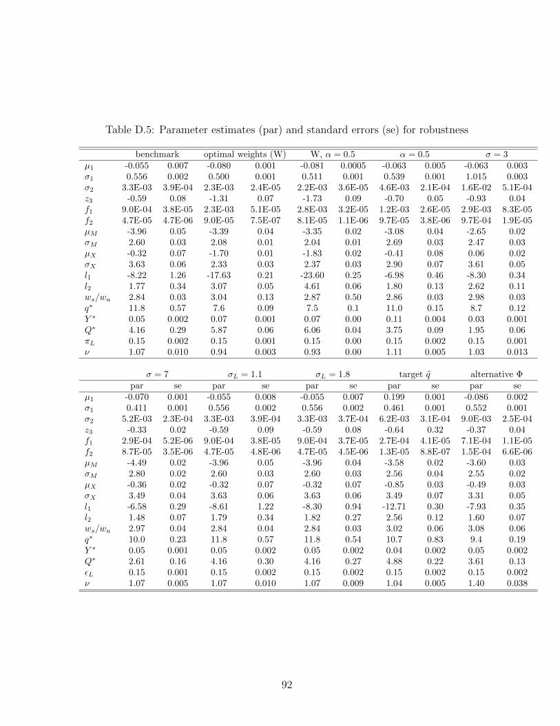
Table D.5: Parameter estimates (par) and standard errors (se) for robustness
benchmark optimal weights (W) W, α = 0.5 α = 0.5 σ = 3µ1 -0.055 0.007 -0.080 0.001 -0.081 0.0005 -0.063 0.005 -0.063 0.003σ1 0.556 0.002 0.500 0.001 0.511 0.001 0.539 0.001 1.015 0.003σ2 3.3E-03 3.9E-04 2.3E-03 2.4E-05 2.2E-03 3.6E-05 4.6E-03 2.1E-04 1.6E-02 5.1E-04z3 -0.59 0.08 -1.31 0.07 -1.73 0.09 -0.70 0.05 -0.93 0.04f1 9.0E-04 3.8E-05 2.3E-03 5.1E-05 2.8E-03 3.2E-05 1.2E-03 2.6E-05 2.9E-03 8.3E-05f2 4.7E-05 4.7E-06 9.0E-05 7.5E-07 8.1E-05 1.1E-06 9.7E-05 3.8E-06 9.7E-04 1.9E-05µM -3.96 0.05 -3.39 0.04 -3.35 0.02 -3.08 0.04 -2.65 0.02σM 2.60 0.03 2.08 0.01 2.04 0.01 2.69 0.03 2.47 0.03µX -0.32 0.07 -1.70 0.01 -1.83 0.02 -0.41 0.08 0.06 0.02σX 3.63 0.06 2.33 0.03 2.37 0.03 2.90 0.07 3.61 0.05l1 -8.22 1.26 -17.63 0.21 -23.60 0.25 -6.98 0.46 -8.30 0.34l2 1.77 0.34 3.07 0.05 4.61 0.06 1.80 0.13 2.62 0.11ws/wu 2.84 0.03 3.04 0.13 2.87 0.50 2.86 0.03 2.98 0.03q∗ 11.8 0.57 7.6 0.09 7.5 0.1 11.0 0.15 8.7 0.12Y ∗ 0.05 0.002 0.07 0.001 0.07 0.00 0.11 0.004 0.03 0.001Q∗ 4.16 0.29 5.87 0.06 6.06 0.04 3.75 0.09 1.95 0.06πL 0.15 0.002 0.15 0.001 0.15 0.00 0.15 0.002 0.15 0.001ν 1.07 0.010 0.94 0.003 0.93 0.00 1.11 0.005 1.03 0.013
σ = 7 σL = 1.1 σL = 1.8 target q alternative Φpar se par se par se par se par se
µ1 -0.070 0.001 -0.055 0.008 -0.055 0.007 0.199 0.001 -0.086 0.002σ1 0.411 0.001 0.556 0.002 0.556 0.002 0.461 0.001 0.552 0.001σ2 5.2E-03 2.3E-04 3.3E-03 3.9E-04 3.3E-03 3.7E-04 6.2E-03 3.1E-04 9.0E-03 2.5E-04z3 -0.33 0.02 -0.59 0.09 -0.59 0.08 -0.64 0.32 -0.37 0.04f1 2.9E-04 5.2E-06 9.0E-04 3.8E-05 9.0E-04 3.7E-05 2.7E-04 4.1E-05 7.1E-04 1.1E-05f2 8.7E-05 3.5E-06 4.7E-05 4.8E-06 4.7E-05 4.5E-06 1.3E-05 8.8E-07 1.5E-04 6.6E-06µM -4.49 0.02 -3.96 0.05 -3.96 0.04 -3.58 0.02 -3.60 0.03σM 2.80 0.02 2.60 0.03 2.60 0.03 2.56 0.04 2.55 0.02µX -0.36 0.02 -0.32 0.07 -0.32 0.07 -0.85 0.03 -0.49 0.03σX 3.49 0.04 3.63 0.06 3.63 0.06 3.49 0.07 3.31 0.05l1 -6.58 0.29 -8.61 1.22 -8.30 0.94 -12.71 0.30 -7.93 0.35l2 1.48 0.07 1.79 0.34 1.82 0.27 2.56 0.12 1.60 0.07ws/wu 2.97 0.04 2.84 0.04 2.84 0.03 3.02 0.06 3.08 0.06q∗ 10.0 0.23 11.8 0.57 11.8 0.54 10.7 0.83 9.4 0.19Y ∗ 0.05 0.001 0.05 0.002 0.05 0.002 0.04 0.002 0.05 0.002Q∗ 2.61 0.16 4.16 0.30 4.16 0.27 4.88 0.22 3.61 0.13εL 0.15 0.001 0.15 0.002 0.15 0.002 0.15 0.002 0.15 0.002ν 1.07 0.005 1.07 0.010 1.07 0.009 1.04 0.005 1.40 0.038
92

Second, we calculate the estimation moments associated with the benchmark parameter
estimates. Then, starting from a random set of parameters we run the optimization algorithm
10 times to search for parameter values that match the estimation moments.63 To estimate the
model, we run both simplex and simulated annealing five times and find that the results are
more precisely estimated with simulated annealing. This is reassuring since the method searches
for the global maximum. Results from the Monte Carlo simulations appear on table E.1. For all
parameters, mean estimates from the simulations are extremely close to the original estimates,
and standard deviations are generally small.
Recall from simulations that, when estimating the model, we hold fixed a vector of uniform
random draws of each firm that are transformed into the firm-specific parameters z1, z2, fM ,
fX and measurement error in labor. When starting each of the 10 searches above, we change
these vectors of random variables. So, results of these Monte Carlo experiments also indicate
that the number of firms simulated 100,000 are sufficiently large so that parameter estimates do
not depend on firm-specific draws. Indeed we confirm, that predicted moments barely change
in the cross section when we change these firm-specific random draws.
Third, the counterfactual with elastic labor supply exogenously changes tariffs t and allows
Y ∗ and p∗ to change to match changes in imports and exports in the data. We check that
the economy moves smoothly from the estimated equilibrium to the counterfactual. We slowly
move (Y ∗, p∗, t) from the estimated model (Y ∗0 , p∗0, t0) to their counterfactual levels (Y ∗1 , p
∗1, t1)
in increments of 1/100 the distance between the two. The choice of quality of some firms jump,
when they change their discrete choices of importing and exporting. But equilibrium functions
P and χ move smoothly with (Y ∗, p∗, t). Across incremental changes in (Y ∗, p∗, t) and all quality
levels in the grid, the mean change in function P was of 0.1% of its original level with a standard
deviation of 0.09%, and the mean change in χ was of 0.2% with a standard deviation of 0.04%.
Similar results hold for the inelastic labor counterfactual when wages are also change. This
result suggests that the transition to the baseline counterfactuals is continuous and that the
economy is not “jumping” to an alternative equilibrium.
63In addition to observed moments, we target the mean of quality choices, q = 4.0. In the originalestimation, we calibrated the mean quality to ensure that quality choices are in q ∈ [0, 10]. We verify thatchanging the mean in a reasonable range barely changes the cross-sectional and counterfactual results.
93
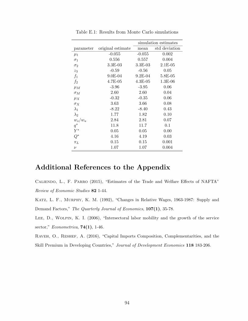
Table E.1: Results from Monte Carlo simulations
simulation estimatesparameter original estimate mean std deviation
µ1 -0.055 -0.055 0.002σ1 0.556 0.557 0.004σ2 3.3E-03 3.3E-03 2.1E-05z3 -0.59 -0.56 0.05f1 9.0E-04 9.2E-04 5.8E-05f2 4.7E-05 4.3E-05 1.3E-06µM -3.96 -3.95 0.06σM 2.60 2.60 0.04µX -0.32 -0.35 0.06σX 3.63 3.66 0.08λ1 -8.22 -8.40 0.43λ2 1.77 1.82 0.10ws/wu 2.84 2.81 0.07q∗ 11.8 11.7 0.1Y ∗ 0.05 0.05 0.00Q∗ 4.16 4.19 0.03πL 0.15 0.15 0.001ν 1.07 1.07 0.004
Additional References to the Appendix
Caliendo, L., F. Parro (2015), “Estimates of the Trade and Welfare Effects of NAFTA”
Review of Economic Studies 82 1-44.
Katz, L. F., Murphy, K. M. (1992), “Changes in Relative Wages, 1963-1987: Supply and
Demand Factors,” The Quarterly Journal of Economics, 107(1), 35-78.
Lee, D., Wolpin, K. I. (2006), “Intersectoral labor mobility and the growth of the service
sector,” Econometrica, 74(1), 1-46.
Raveh, O., Reshef, A. (2016), “Capital Imports Composition, Complementarities, and the
Skill Premium in Developing Countries,” Journal of Development Economics 118 183-206.
94