Trade, Pollution and Mortality in China

Matilde Bombardini (UBC, CIFAR and NBER),

and Bingjing Li (National University of Singapore)

Oct 2019

Abstract

Did the rapid expansion of Chinese exports between 1990 and 2010 contribute to thecountry’s worsening environmental quality? We exploit variation in local industrial compo-sition to gauge the effect on pollution and health outcomes of export expansion due to thedecline in tariffs faced by Chinese exporters. In theory, rising exports can increase pollutionand mortality due to increased output, but they may also raise local incomes, which can inturn promote better health and environmental quality. The paper teases out these competingeffects by constructing two export shocks at the prefecture level: (i) the pollution contentof export expansion; (ii) export expansion in dollars per worker. We find that the pollutioncontent of exports affects pollution and mortality: a one standard deviation increase in theshock increases infant mortality by 4.1 deaths per thousand live births, which is about 23%of the standard deviation of infant mortality change during the period. The dollar value ofexport expansion reduces mortality by 1.2 deaths, but the effect is not statistically significant.We show that the channel through which exports affect mortality is pollution concentration.We find a negative, but insignificant effect on pollution of the dollar-value export shocks,a potential “technique” effect whereby higher income drives demand for clean environment.Finally, we find that only infant mortality related to cardio-respiratory conditions respondsto exports shocks, while deaths due to accidents and other causes are not affected.

We would like to thank Werner Antweiler, David Autor, Davin Chor, Brian Copeland, ArnaudCostinot, Alastair Fraser, David Green, Ruixue Jia, Hiro Kasahara, Keith Head, Vadim Marmer,Peter Morrow, Salvador Navarro, Tomasz Swiecki and seminar participants at CIFAR, DartmouthTuck School of Business, Econometric Society Asian Meeting, Hong Kong University of Science andTechnology, Johns Hopkins SAIS, LSE, McMaster Workshop in International Economics, NationalUniversity of Singapore, UCLA, UC San Diego, University of Virginia, the West Coast Trade Work-shop and the NBER Summer Institute for helpful comments. Bombardini acknowledges financialsupport from CIFAR and SSHRC.

1 Introduction

Among the many dimensions of China’s economic growth in the last 3 decades is the contempo-

raneous boom in export performance: the annual export growth rate was 14% during the 1990s

and 21% during the 2000s. This rapid economic growth has been accompanied by concerns that

many of the benefits deriving from higher incomes may be attenuated by the similarly rapid dete-

rioration in the environment and increase in pollution.1 This paper studies how the export boom

in China between 1990 and 2010 affected pollution and infant mortality across different Chinese

prefectures. The specific question we tackle is whether areas that were more involved in the export

boom witnessed a deterioration or improvement in pollution and health outcomes relative to less

exposed areas. This is ex ante unclear as an export boom brings about more production and

therefore pollution (the “scale” effect in Copeland and Taylor, 2003), but also higher incomes,

which may affect both pollution and health outcomes in the opposite direction.2

We capture these potentially opposite channels through two export exposure shocks. For

each Chinese prefecture we construct: (i) PollExShock, which represents the pollution content of

export expansion and is measured in pounds of pollutant per worker; (ii) ExShock, which measures

the dollars per worker associated with export expansion. The variable ExShock measures the

extent to which a prefecture is initially specialized in industries that subsequently experience a

large export increase. The variable PollExShock captures the interaction of export expansion and

pollution intensity: prefectures with larger initial employment in industries that both experience

large export shocks and have high emission intensity are expected to become more polluted. The

two measures differ because prefectures specialize in different products and while two prefectures

may experience the same export shock in dollar terms, the one specializing in a polluting sector,

like steel, experiences a larger PollExShock.

There are two key features of these measures. First, they rely on variation across prefectures

in the initial pattern of comparative advantage across industries, similarly to the approach by

Edmonds et al. (2010), Topalova (2010), Kovak (2013) and Autor et al. (2013) to study the effects

of import competition on employment. The second feature is that, differently from these studies,

here we are interested in the effect on China of the export demand shock generated by the rest of

the world. The paper therefore builds an export expansion measure that captures the portion of

China’s export increase that is predicted by the change in tariffs faced by Chinese exporters over

time in different sectors.

Why are we interested in this specific component of export and of output growth more in

general? In general, production for both domestic consumption and exporting responds to a

1According to Ebenstein et al. (2015) many of the gains in health outcomes have been slowed down by asimultaneous rise in the concentration of pollutants.

2Again, in the language of Copeland and Taylor (2003) and Grossman and Krueger (1995), holding constantthe implied total emissions due to increased exports, higher revenues from exports may result in lower pollutiondue to a “technique” effect by which demand for a clean environment rises with income.

1

multitude of shocks. These include the national-level supply shocks, like productivity innovations

and institutional changes, as well as demand-side shifters, each of which may affect emissions

differently. Were we to simply consider the correlation between emissions and output, we would

not be able to easily interpret it. The paper therefore focuses on a specific dimension of aggregate

demand where this identification problem is alleviated. It makes use of the presence of externally

imposed tariffs, thus isolating foreign demand shocks from other unobserved sources of output

dynamics.

We employ the shift-share approach instead of actual export expansion, to identify the causal

relationship running from tariff-predicted export expansion to local environmental and health

outcomes. At the prefecture level, there could be numerous supply shifters that simultaneously

affect export performance and environmental/health outcomes. For example, a weakening in

the enforcement of environmental regulations may increase local exports by reducing production

costs, but this may also lead to environmental degradation and worsening health outcomes. By

not employing export growth at the local level, but rather using a weighted average of national

export expansion with the weights determined by the initial industry composition, the shift-share

design helps purging such potential confounding factors.

Magnitudes are substantial. We find that a one standard deviation increase in PollExShock

increases infant mortality by an additional 4.1 infant deaths per one thousand live births, while a

one standard deviation increase in ExShock decreases infant mortality by a statistically insignif-

icant 1.2 infant deaths.3 The size of these effects has to be gauged in the context of the evolution

of infant mortality over this period. In our data, between 1990 and 2010 infant mortality rate

in China went from 36 per thousand to 5 deaths per thousand live births, but this decline hides

substantial heterogeneity. Between 2000 and 2010 for example, the 75th percentile prefecture

experienced a decline of 23.7 deaths, while the 25th percentile prefecture saw a drop of only 8.7

deaths. The effect of ExShock not only is insignificant, but is only equivalent to 6.6% of such

standard deviation.

In two different exercises we calculate the overall effect of the two shocks and illustrate that

both at the national level and at the provincial level export expansion had primarily a negative

effect, i.e. very few prefectures had a net improvement in health outcomes. Ignoring a potentially

beneficial effect of trade common to all prefectures that our cross-prefecture approach necessarily

nets out, we calculate that an extra 803,088 infant deaths during the 1990-2010 period are due

to export expansion. Importantly, using the same data as Chen et al. (2013), we can show that

the negative effects of trade on health are concentrated in mortality due to cardio-respiratory

conditions, which are the most sensitive to air pollution, corroborating our findings.

How do PollExShock and ExShock affect mortality? The next question we tackle is the

quantification of the channels through which these two shocks influence health outcomes. The

3We find that ExShock tends to decrease mortality, but the effect is statistically significant only during thedecade 2000-2010 (during which export expansion was an order of magnitude bigger than during the 1990’s).

2

most intuitive way in which PollExShock affects mortality is through pollutant concentration.

Instead ExShock may affect mortality through different channels.4 Our identification relies on

the assumption that conditional on ExShock, PollExShock affects mortality only through the

channel of air pollution. We show that a positive PollExShock increases the concentration of

SO2, while ExShock tends to reduce it. In the decade 2000-2010 a one standard deviation in-

crease in PollExShock increases SO2 concentration by 6.3 µg/m3 while a one standard deviation

increase in ExShock decreases SO2 concentration by 2.1 µg/m3 (this latter effect is not statisti-

cally significant). These changes represent respectively 19% and −6.3% of the standard deviation

of SO2 concentration change during 2000-2010.5 We have two possible explanations for the lack of

a strong income effect of export expansion on both mortality and pollution. The first one has to

do with the fact that environmental policy is set centrally in China and local increases in income

may not directly translate into local changes in policy.6 The second potential explanation is based

on other consequences of income growth that may be associated to increased pollution, such as

the increase in vehicle ownership (see Dargay et al. 2007).

Finally, the paper shows how pollution affects infant mortality, a link which has been studied in

the previous literature, but for which we offer a novel identification strategy. We find the elasticity

of infant mortality to SO2 to be 0.81. This is quantitatively similar to the estimate by Tanaka

(2015) of 0.82 for China (albeit during a different time period). The elasticity of IMR to PM2.5 is

1.9.7

We are careful in addressing a series of issues that may affect confidence in these results.

Importantly, like all studies employing a shift-share approach, our paper faces the challenge of

establishing that the results are not simply due to the initial pattern of industrial specialization.

It is plausible for example to hypothesize that prefectures initially specialized in dirty industries

would experience a relative increase in mortality over this period even without export shocks.

This issue is at the heart of Goldsmith-Pinkham et al. (2018), who emphasize how, with Bartik-

style variables, identification relies on the exogeneity of the initial industry shares. We calculate

Rotemberg weights as proposed by Goldsmith-Pinkham et al. (2018) in Appendix F.2, and show

that: i) they are less concentrated in a few industries relative to Autor et al. (2013) and ii) there are

no pre-trends in infant mortality associated with the employment share of high Rotemberg weights

4On the one hand, an increase in income due to export expansion may increase the demand for clean environmentand the consumption of healthcare services which would in turn improve health outcomes. On the other hand,it may also increase the consumption of environmentally unfriendly goods like cars, which would in turn raisepollution.

5We also find that PM2.5 concentration induced by a standard deviation increase in PollExShock is µg/m3,which amounts to 17.7% of the standard deviation of the decadal change in PM2.5 concentration. The correspondingnumbers for a standard deviation increase in ExShock are -1.6 µg/m3 (not statistically significant) and 16.8%,respectively.

6See Hao et al. (2007) for a description of the national policies adopted over the last three decades.7This is not directly comparable to the estimate of 1.73 we have for China by Chen et al. (2013) because the

pollutant in that case is total suspended particles. A potential explanation of this larger effect is that PM2.5 isconsidered much more fatal due to the smaller diameter of the particles.

3

industries. We also perform the “balance” checks proposed under the alternative identification

assumptions discussed by Borusyak et al. (2018) and show that at the industry level, pollution

embodied in exports is uncorrelated with industry-specific weighted average of other local shocks

such as changes in educational attainment, health expenditure proxies etc. Aside from these formal

checks, in the paper we also control for pre-existing trends and present placebo tests as customary

in this literature.

Because concerns about initial industrial specialization are so important for the identification

and quantification at the core of this paper, in what follows we present a graphical exercise that

serves two purposes. First, it addresses in an intuitive way the key concern that having a high

employment share in a dirty industry is entirely responsible for the subsequent increase in infant

mortality, regardless of trade shocks. Second, it illustrates the basic nature of the exercise, which

is analogous to a continuous difference-in-differences as clarified by Goldsmith-Pinkham et al.

(2018). Simply having high employment shares in dirty industries is not enough to predict a high

increase in mortality. A prefecture must have a high employment share in an industry that has

both high emission intensity and high trade exposure. Even though we present all data details

later, we construct a measure that simply classifies sectors according to two criteria: dirty/clean

(D and C) and high-export-growth/low-export-growth in the decade 2000-10 (H and L).8 We then

obtain employment shares in 2000 for each prefecture in each of the 4 groups of industries (CH,

DH, CL and DL). Panel A of Figure 1 plots the change in infant mortality rate (IMR) for each

prefecture in 2000-2010 against the following relative employment ratio in the year 2000:

EmpShare(DH)

EmpShare(CH) + EmpShare(DH).

Figure 1 shows that IMR increased in prefectures that initially had a relatively higher employment

in dirty industries that also saw high export growth in 2000-10. Conversely, Panel B of Figure 1

presents the same change in IMR against the analogous employment ratio for low-export-growth

industries:EmpShare(DL)

EmpShare(CL) + EmpShare(DL).

Figure 1 shows that initial specialization in dirty sectors does not predict change in infant mortality

rate when we focus on low export growth industries.

The paper reports a number of other checks to probe our results. For example, we address the

potential objection that official sources for data on pollution may misreport pollutant concentra-

tions in order to hide imperfect compliance with environmental regulation from the public. In this

regard we check the correlation of the official daily pollution levels with the levels reported by the

American Embassy and Consulates in five Chinese cities. We show that the correlation is above

8Dirty and Clean industries are grouped according to whether the sectoral value of emission intensity is aboveor below the median. The high-export-growth (low-export-growth) industries are the ones belonging to upper(bottom) tercile of export growth per worker. More details can be found in Appendix C.

4

94 percent. Another issue that we delve on is the quantitative importance of trade policy shocks

for the overall structure of production and level of pollution. We take a specific episode, the steel

safeguard tariffs imposed by the US in 2002-2003 to show that, for prefectures with heavy steel

production, pollution decreases relative to control prefectures in 2001 and increases back up in

2003.9 Finally, we check the robustness of our results to alternative measures of export shocks

that take into account shocks in neighboring and upwind prefectures, import shocks, input-output

linkages that transmit foreign demand shocks to upstream industries, and control for local energy

production among other socio-economic determinants of mortality and pollution. We also analyze

the results by gender and by age, finding a relatively homogeneous effect across different groups.

1.1 Relation to the Literature

Our study contributes to three main strands of the literature, the one related to trade and pollu-

tion, the one studying the effect of pollution on mortality and finally, the broader area exploring

the effect of international trade at the local level. The first generally addresses the question of

whether international trade affects pollution through a variety of channels. Employing the lan-

guage introduced by Grossman and Krueger (1995), Copeland and Taylor (2003) and Copeland

and Taylor (2004), increased international trade can: i) lead to a more intense scale of production

which increases pollution (scale effect) ; ii) induce specialization, which could reduce or increase

pollution depending on whether a country specializes in clean or dirty industries (composition

effect); and iii) generate an increase in income which would raise the demand for better environ-

mental quality (technique effect). Antweiler et al. (2001) find that emissions across several world

cities depend positively on the scale of economic activity and the capital abundance of the country

and depend negatively on income. Their main finding in relation to the trade-environment link

is that, as a country is more open to trade, on average emissions are lower. Their cautiously

optimistic conclusion is that trade may be good for the environment, but they note that the effect

of trade in different countries depend on their pattern of comparative advantage. Although their

study employs a panel data set that allows them to control for time invariant country effect, the

authors themselves admit that the issue of identification due to the presence of unobserved shocks

is not fully solved in their paper. A different approach to identification is offered by Frankel

and Rose (2005), although they limit their analysis to a cross-section of countries and employ a

geography-based IV approach. They identify that, controlling for income, increased trade leads

to lower emissions. Our contribution is to take a step further in the direction of identifying the

causal effect of trade on environmental quality and health. Our within-country approach neces-

sarily controls for several unobserved variables that are not accounted for by country-level panel

studies. We also adopt several techniques to deal with other potential sources of endogeneity. The

cost of our approach, relative to country-level analysis, is that we necessarily ignore national-level

9The results of this event study is reported in Appendix A.

5

general equilibrium effects and therefore we will not be able to conclusively say whether China as

a whole saw its environmental quality improve or worsen because of trade expansion.

In a recent contribution Shapiro and Walker (2018) conclude that trade has not played a

quantitatively significant role in explaining the large decline in emissions in the US between 1990

and 2008. Detailed plant-level data allows them to pin most of the change in emissions on within-

plant changes in techniques of production. Other recent contributions have focused on the firm-

level link between exporting and emissions. In the cross-section Forslid et al. (2018) find that

exporters tend to have lower emission intensities, while Cherniwchan (2017) finds lower emissions

as firms are exposed to tariffs cuts in the output market. Interestingly, Barrows and Ollivier

(2018) find that this effect is solely due to a change in the product mix: for the same product,

exporters do not reduce emissions per unit, but they concentrate production on their core and

cleaner products. Because our emission data are available only at the aggregate level, we cannot

investigate potentially interesting effects of trade opening on the technique of production at the

local level, but when we consider the total effect at the prefecture level, we should keep in mind

that these mechanisms may also be at play.

Our paper also relates to another strand of literature that studies the impact of pollution on

mortality, in particular of infants. The reason why infant mortality is often chosen as a relevant

outcome is not only that young children are particularly vulnerable members of society which

per se may be of particular interest, but also because their health outcomes are more closely

related to immediate environmental conditions, while adults’ health may be the consequence of

factors accumulated over the course of many years. These studies are conducted both in developed

countries like Chay and Greenstone (2003a), Chay and Greenstone (2003b), Currie and Neidell

(2005) and Currie et al. (2009), and in developing countries, like Greenstone and Hanna (2014),

Arceo et al. (2016) and (McCaig, 2011).

In terms of specific studies on trade and pollution in China, we are only aware of a few papers,

but none with the same focus as ours. An earlier paper by Dean (2002) considers the link between

openness and water pollution across Chinese provinces, but it essentially exploits national-level

measures of openness and therefore estimates the relationship using pure time variation whereas

our entire strategy relies on exploiting differential shocks within China. de Sousa et al. (2015)

exploit city-level variation in exports and find that increased processing trade in China leads to

lower pollution. They focus more on the role of the international segmentation of production,

and they do not consider the consequences of trade for infant mortality. In the energy and

environmental science literature, Lin et al. (2014) and Yan and Yang (2010) have addressed the

global impact of China’s trade on various pollutants, but they do not identify the effect on China

itself and its air quality; Jiang et al. (2015) use atmospheric and air quality models to compute

the pollution content of China’s exports and an epidemiological model to estimate its effect on

mortality in different provinces, whereas we adopt econometric techniques to identify the causal

effects of export demand shocks with finer data. Another related literature explores the association

6

between China’s economic development and environmental/health outcomes (e.g., Grigoriou et

al. (2005), Ebenstein et al. (2015), Zheng and Kahn (2017)). We complement these studies by

focusing on export expansion, an important driver of China’s economic growth, and on identifying

the causal linkages.10

This paper also connects the rapidly growing literature that employs the variation in ini-

tial regional differences in industry composition to study the differential effects of trade on local

economies within a country. One strand of work focuses on import competition, including Ed-

monds et al. (2010), Topalova (2010), Autor et al. (2013), Kovak (2013), Acemoglu et al. (2016),

Kovak and Dix-Carneiro (2017), among others. The other strand of this literature investigates the

effects of export opportunities on various outcomes, including child labor (Edmonds and Pavc-

nik, 2005), labor market adjustment (Brambilla et al., 2012), poverty reduction (McCaig, 2011),

and employment (Feenstra et al., 2019). Recent work by Erten and Leight (2019) and Facchini

et al. (2019) finds that export expansion due to the reduction in trade policy uncertainty has a

substantial impact on China’s labor market. Aligned with these studies, our paper studies export

demand shocks, but focuses on its effects on environmental and health outcomes. Importantly, we

propose a new formulation of the Bartik-style instrument to separately identify the export-induced

pollution effect and income effect.

The rest of the paper proceeds as follows. Section 2 describes the various data sources, while

Section 2.5 probes the quality of specific variables, like air quality and mortality. In Section 3 we

construct our export shock measures and present our identification strategy in two parts: i) we

first show the reduced form effect of PollExShock and ExShock on mortality; ii) we then show

that export shocks affect mortality through pollution. Section 4 discusses our main results and

reports a number of robustness checks. We conclude in Section 5.

2 Data

This section describes the main sources of data for exports, tariffs, mortality, emission intensity

and pollution. Additional variables are described in Appendix C.

2.1 Local Economies and Employment Data

The unit of analysis is a prefecture in China, which is an administrative division ranking between

province and county. Prefectures are matched across census years according to the 2005 admin-

istration division of China, so that the data have a geographic panel dimension. There are 340

prefectures, with median land area of 13,152 km2 and median population of 3.2 million in year

10There is also an extensive body of work on the effects of pollution on health in China’s context, including Chenet al. (2013), Tanaka (2015), He et al. (2016), among others. In section 4.4, we will revisit this literature when wecompare our estimated effect of air pollution on IMR with the findings in the existing literature.

7

2000. The information on industry employment structure by prefecture is from the 1% sample

of the 1990 and 2000 China Population Censuses. Census data contain relevant information re-

garding the prefecture of residence and the industry of employment at 3-digit Chinese Standard

Industrial Classification (CSIC) level.11

2.2 Export and Tariff Data

From the UN Comtrade Database, we obtain data on China’s export and import values at the

4-digit International Standard Industrial Classification (ISIC) Rev.3 code level for the years 1992,

2000 and 2010.12 Data on export tariffs faced by Chinese exporters by destination countries and

4-digit ISIC Rev.3 industries are from the TRAINS Database.13 We construct the industry-level

tariff rates faced by Chinese exporters, which is the weighted average of tariffs imposed in different

destination markets:

ExTariffkt =∑j

Xjk,t−1

Xk,t−1

τjkt .

Here, τkjt denotes the tariff imposed by country j on good k during the period t. The weights are

determined by the country’s share in China’s total exports of good k in the lag period, and they are

constructed using the trade flow data from three years earlier. As is shown in Table A.2, on average

ln(1+ExTariff) drops from 0.071 by 0.02 log point over the period 1992-2000. The corresponding

numbers for 2000-2010 are 0.051 and 0.015. More importantly, there is substantial variation in

tariff cuts. The standard deviations are 0.047 and 0.032 for the two decades, respectively. We map

trade and tariff data to the 3-digit CSIC sectoral employment data from the population censuses,

using a concordance between ISIC and CSIC.

2.3 Pollution Data

2.3.1 Industry Pollution Intensity

We construct pollution intensity for each 3-digit CSIC industry, using data from the World Bank’s

Industrial Pollution Projection System (IPPS) and China’s environment yearbooks published by

the Ministry of Environmental Protection (MEP). The IPPS is a list of emission intensities, i.e.,

emission per dollar value of output, of a wide variety of pollutants by 4-digit SIC industry. These

data were assembled by the World Bank using the 1987 data from the US EPA emissions database

and manufacturing census.14 We aggregate the data to the 3-digit CSIC level and consider the

pollutants sulfur dioxide (SO2), total suspended particles (TSP ) and nitrogen dioxide (NO2) in

11The 1990 Census employs CSIC 1984 version and the 2000 Census employs the CSIC 1994 version. We reconcilethe two versions and create a consistent 3-digit CSIC code. There are 148 industries in the manufacturing sector.

121992 is the first year when the export data is available for China at 4-digit ISIC level.13We collect both applied and MFN tariffs.14To our best knowledge, there is no analogous data at such disaggregated level for China.

8

the analysis. To address the concern that China’s industrial pollution intensities may be uniformly

higher than those of the US, we use the MEP data on 2-digit sector pollution intensity to adjust

the level. Therefore, while the level of industry pollution intensity is aligned with the MEP data,

the within sector heterogeneity retains features of the IPPS data. See Appendix C.3 for details.

2.3.2 Data on Pollution Concentration

Information on annual daily average concentration of SO2 is collected for the years 1992, 2000

and 2010. The data are obtained from China’s environment yearbooks, which report the data on

air pollution for 77, 100, and 300 cities/prefectures for years 1992, 2000 and 2010, respectively.15

We supplement this main dataset with the information gathered manually from provincial/city

statistical yearbooks, government reports and bulletins. Restricting to prefectures with at least

two readings, we compile an unbalanced panel which covers 203 prefectures.

Satellite information on PM2.5 comes from NASA.16 The NASA dataset contains information

on the three-year running mean of PM2.5 concentration for a grid of 0.1 degree by 0.1 degree

since 1998. Adjacent grid points are approximately 10 kilometers apart. For the purpose of our

analysis, we employ the data of years 2000 and 2010 and construct the decadal change in PM2.5

concentration at the prefecture level. 17

2.4 Mortality Data

Infant mortality rates (IMR) are constructed from the China Population Censuses for years 1982,

1990, 2000 and 2010. Each census records the number of births and deaths within a household

during the last 12 months before the census was taken (details in Appendix C.4). The total

number of deaths at age 0 is collected for every county, and then aggregated to the prefecture

level. The total number of births by prefecture is derived in the same way. The infant mortality

rate is defined as the number of deaths at age 0 per 1000 live births. In addition to IMR, we

assemble data on the mortality rate of young children aged 1-4 at the prefecture level for the years

1990, 2000 and 2010.18

We supplement the census mortality data with vital statistics obtained from the China’s Disease

Surveillance Points (DSP) system for years 1992 and 2000. The DSP collects birth and death

15Only SO2 concentration level data are continuously published in China’s environmental yearbooks over thesample period. The concentration of TSP was reported in 1992 and 2000, however, it was replaced by PM10 in2010.

16We use the Global Annual PM2.5 Grids from MODIS, MISR and SeaWiFS Aerosol Optical Depth (AOD), v1(1998-2012) dataset from NASA’s Socioeconomic Data and Applications Center (SEDAC). The data on PM2.5 arederived from Aerosol Optical Depth satellite retrievals, using the GEOS-Chem chemical transport model, whichaccounts for the time-varying local relationships between AOD and PM2.5.

17Specifically, for each county-year observation, we calculate the average PM2.5 concentration using the dataof the grid points that fall within the county. Then the county-level data is aggregated to the prefecture level,weighted by the county population.

18The mortality rate of young children aged 1-4 is defined as Deaths1−4

Deaths1−4+Poplution1−4× 1000.

9

registration for 145 nationally representative sites, covering approximately 1% of the national

population.19 The data recorded whether or not an infant died within a calendar year and the

cause of death, using International Classification of Disease 9th Revision (ICD-9) codes.

2.5 Quality Assessment of the Chinese Data on Pollution and Mortal-

ity

In this section we address the concern that official reports from the Chinese government may not

be reliable due to the desire to under-report pollution and mortality. With regards to pollution,

in order to assess the severity of underreporting, we have to consider the incentives of officials at

various levels of government in the period considered, between 1990 and 2010. As reported by

Chen et al. (2013), although the data on pollution were collected starting in the late 1970’s, they

were not published until 1998, so it is unlikely that fear of public uproar would be a concern for

local officials. More importantly, in a number of studies Jia (2012) and Jia et al. (2015) report

that officials most likely perceived local economic growth to be the criterion for promotion, rather

than environmental quality. In fact, Jia (2012) shows how increased pollution is a byproduct

of the quest for higher economic growth by ambitious politicians. Moreover, our identification

strategy compares the changes in pollutant concentration of prefectures with different initial in-

dustrial specialization. Therefore, our results will be contaminated only if the pollution data were

systematically manipulated for prefectures with different initial industry composition. Despite all

these considerations, one might still be concerned that our pollution measures are very noisy, so in

Appendix D we corroborate our data by showing that the official Chinese daily data on air quality

has a correlation of at least 0.94 with the US Consulate or Embassy data, depending on the city.

In Appendix D we also show the results of an exercise aimed at detecting over- or under-

reporting of infant mortality. In essence we compare the number of 10-year-old children in a

prefecture in a given census year with the expected number of 10-year-old children based on the

reported mortality and birth figures from the last population census (a decade earlier). We find a

correlation of 0.98 between these two measures, which of course cannot perfectly coincide due to

unaccounted-for migration.

3 Empirical Specification

In this section we lay out the empirical methodology and explain our identification strategy. Figure

2 illustrates schematically the causality links that this paper explores. “Export” tariffs, i.e., tariffs

that Chinese exporters face, affect the extent of export expansion and the pollution embodied,

19The surveillance sites are primarily at the county level. We match the surveillance sites to 118 prefectureswhere they are located.

10

measured by ExShock and PollExShock, which ultimately affect mortality, through pollution

concentration. We delve into the measures and mechanism further below.

3.1 Pollution Export Shock and Export Shock

In this section we build empirical measures that capture exports shocks based on the derivation

in Appendix B. We expect increased exports to affect pollution through two potential channels,

which we capture with two types of export shocks.

i) PollExShockit - Increased foreign demand induces an increase in total manufacturing pro-

duction, but the direct environmental consequences depend on whether the export expansion

is concentrated in dirty or clean industries.

ii) ExShockit - Increased exports may also increase local wages and profits, which, through an

income effect, may increase the demand for clean air, thus reducing pollution. Although this

income effect is ignored by our model in Appendix B, we believe it must be accounted for

in the empirical analysis.

We focus more on channel i) first. As detailed in Appendix B, in what follows we assume that

increased exports due to higher demand in the rest of the world were produced by labor primarily

moving from rural to urban areas and that was previously employed in subsistence agriculture,

rather than industrial production for the domestic market. Conditional on data availability for

prefecture-level exports across all years in the sample, we could find the impact of export expansion

on local pollution change using the following equation:

∆Cpit =

∑k

γpkt∆Xikt

Li, (1)

where ∆Cpit measures the change in concentration of pollutant p in prefecture i between year

t− 1 and year t, γpkt is the pollution intensity for pollutant p,20 ∆Xikt is the analogous change in

export value from prefecture i in sector k, and Li denotes the size of prefecture i. Without this

normalization by prefecture size, the following example would pose a problem. Imagine that two

unequally-sized prefectures face the same total increase in emissions. If we did not normalize by

prefecture size, we would attribute the same increase in pollutant concentration to both, whereas

the smaller prefecture is in fact facing a larger increase in such concentration. In practice we

approximate the size of the prefecture with total employment and note that this normalization

does not qualitatively affect our results (see Table 5).

Prefecture-level exports could in principle be calculated from firm-level customs data, but such

data are not available for the earlier time period in our sample. Therefore we exploit the model

20Specifically, γpkt =Pp

kt

Ykt, where P pkt is the total amount of emissions in sector k and Ykt is the value of output.

11

prediction in equation (19) to approximate ∆Xikt asXik,t−1

Xk,t−1∆Xkt, where ∆Xkt is the change in

export from China to the rest of world of industry k in period t. We use employment shareLik,t−1

Lk,t−1,

where Lik,t−1 and Lk,t−1 are respectively prefecture i’s employment and China’s total employment

in industry k at the beginning of the period, to proxy for a prefecture’s export share in industry k,Xik,t−1

Xk,t−1. This is, again, because export data at the prefecture level are not available for the earlier

time period (1990) of our sample.21

In summary, PollExShockpit, our empirical measure of export-induced pollution in prefecture

i, is constructed as follows:

PollExShockpit =∑k

γpktLik,t−1

Li,t−1

∆Xkt

Lk,t−1

, (2)

and it measures the pounds of pollutant p associated with export expansion measured on a per

worker basis. The normalization by local employment that we discussed above serves the additional

purpose of making our PollExShockpit measure easily comparable to our second measure of export

shock, which we define simply as ExShockit. This second measure, which addresses channel ii),

i.e. the impact of export-induced income growth on environmental outcomes, is constructed as

follows:

ExShockit =∑k

Lik,t−1

Li,t−1

∆Xkt

Lk,t−1

, (3)

and it measures the dollar value of export expansion in prefecture i, on a per worker basis.

Importantly the two shocks measure different dimensions of export expansion. While ExShockit

measures the total value of all goods being exported, PollExShockpit gives different weights to

different sectors according to their emission intensity.

The variable ExShockit is the equivalent of the change in value of imports per worker at the

commuting zone level in Autor et al. (2013). The variation across prefectures of our two mea-

sures, PollExShockpit and ExShockit stems from initial differences in local industry employment

structure, a feature common to the Bartik approach (see Bartik, 1991). We analyze more in detail

the properties of these shocks in the context of our discussion of identification, which we cover in

Section 3.2.1.

21We adopt different approaches to investigate the potential bias introduced by this approximation. First, inSection 4.3.3, we construct the theoretically consistent measures using the export share data in 2000, and findregression results aligned with the baseline findings. Second, in Appendix E, we regress a prefecture’s exportshare XiRk

XCRkon its employment share Lik

LCk, using the data in 2000. The estimated coefficient is 0.965, insignificantly

different from one. Under the condition that the discrepancy between export and employment shares is uncorrelatedwith a prefecture’s export composition, our estimates provide lower bounds for the effects of export shocks onpollution and IMR.

12

3.2 Specification 1: Total Effect of Export Shocks on Mortality

In this section we describe our approach to identifying the causal impact of a decline in trade costs

on pollution and mortality across prefectures in China. Our first specification is the following:

∆IMRit = α1PollExShockpit + α2ExShockit + φrt + εit (4)

where ∆IMRit is the change in infant mortality rate in prefecture i between year t − 1 and t,

while εit is an error term that captures other unobserved factors and is assumed to be orthogonal

the two export shocks. The regression stacks the first differences of two periods, 1990 to 2000 and

2000 to 2010. The stacked difference model is similar to a three-period fixed effect model, and

removes any time-invariant prefecture-specific determinants of health outcomes. We add to this

first-difference specification Region × Y ear fixed effects, φrt, to account for differential trends in

mortality rate changes across 8 macro regions in China (this is comparable, but more demanding

than, the Census division fixed effects in Autor et al. (2013)’s stacked first-difference model). In

the following section we address issues related to endogeneity.

3.2.1 Identification Strategy

Our basic specification (4) relates infant mortality to our two export shocks, ignoring other po-

tential socio-economic determinants that could be important drivers of mortality. We therefore

include several control variables that capture education, provision of health services and ethnic

composition. Even after the inclusion of such variables, we are still concerned that the error term

εit may be affected by other factors that are correlated with our export shock measures.

Bartik Approach

The first type of shocks we may be concerned about is local productivity or factor supply changes

that may affect local output and exports and affect pollution concentration at the same time.

Both measures PollExShockpit and ExShockit, through a Bartik approach, tackle this issue by

not employing export expansion at the local level, but rather using a weighted average of national

export expansion. As usual, this approach relies on the assumption that other time-varying, region-

specific determinants of the outcome variable are uncorrelated with a prefecture’s initial industry

composition. As discussed in the introduction, we view this as a the key threat to identification

and we address the issue in many ways. The first approach is to control for pre-existing trends in

infant mortality, so that we can account for the possibility that a prefecture initially specialized

in polluting industries may be on a different trajectory in terms of overall health outcomes. The

second approach is to check that we cannot predict current infant mortality changes using future

export shocks, thereby again ensuring that the two are not driven by a common unobserved factor.

13

Our third approach is to control for the following variable, PollEmpl, which measures the level

of pollution implied by the initial employment structure in prefecture i:

PollEmplpit =∑k

γpktLik,t−1

Li,t−1

. (5)

Essentially we are concerned that regions initially specialized in dirty industries may just have

initially more lax regulation and therefore be prone to relax such regulations even more. We may

then mistake such effect as the consequence of export expansion. Controlling for PollEmpl makes

sure that we are comparing two prefectures with the same initial average level of specialization in

dirty industry, which likely summarizes their attribute towards regulation, among other factors.

Consider two prefectures specializing, respectively, in steel and cement and assume the two sectors

have very similar pollution intensities. As a result, the two prefectures have a similar value of

PollEmpl, indicating they have similar initial pollution level. Nevertheless, they may experience

different PollExpShock, if for example, steel receives a larger external demand shock.

The fourth approach is to more formally calculate the “Rotemberg weights” associated with

each industry as suggested by Goldsmith-Pinkham et al. (2018). In Appendix F.2 we show that the

Rotemberg weights, which measure the importance of each industry in determining the coefficient

of interest and the coefficient’s sensitivity to misspecification in each industry share, are less

concentrated in a few industries relative to Autor et al. (2013) and that there are no systematic

pre-trends in infant mortality associated with the employment shares of industries with high

Rotemberg weights.22

The fifth approach is to take the complementary view of the identification requirements pro-

posed by Borusyak et al. (2018). In that paper the identification condition is that the industry-level

shock is uncorrelated with a weighted average of the unobservable local unobserved shocks, with

the weights reflecting the importance of the industry in the local economy. Following this logic, in

Appendix F.4 we perform the “balance” test suggested by Borusyak et al. (2018) and show that

a weighted average of observable local shocks (e.g. the change in skill level and migrant share) is

uncorrelated with PollExShock at the industry level. The test shows that ExShock is instead

correlated with some of these averages of local shocks and confirms that we need to control for

changes in various socio-economic factors, such as migrant share, skill composition and share of

population in agriculture.

Finally, there may be a concern that a high initial employment share in dirty industries may be

correlated with the tendency to employ more migrant workers, whose children may systematically

have worse health outcomes. Perhaps surprisingly, polluting industries do not systematically

employ more migrant workers as a share of their total employment. The first two columns of

Table 2 show that pollution intensity is negatively correlated with the share of cross-prefecture

22As another robustness check, we implement a related suggestion by Goldsmith-Pinkham et al. (2018) bydropping one 2-digit sector at a time in Table A.8.

14

migrants in the industry and uncorrelated with the share of workers with rural hukou (a plausible

proxy of lower socio-economic status migrants). Given these correlations, the concern that our

estimates may be driven by selective migration should be alleviated.

Export Tariffs and Export Shocks

A separate issue from the one related to exogeneity of industry shares is what goes into the national

shock that form the Bartik instrument. The typical concern here is that in a finite sample the

export expansion at the national level can be driven by a few prefectures which highly specialize

in an industry. Goldsmith-Pinkham et al. (2018) suggest a leave-one-out estimator to address this

issue, while Autor et al. (2013) employ exports from China to other developed countries to build

their Bartik instrument. The second method is preferable if we believe that supply shocks may be

correlated geographically. In our context we believe tariffs faced by Chinese exporters can serve

this purpose.

A more fundamental reason why we consider tariff-predicted exports is a clean interpretation

of the results as the health consequences of foreign demand shocks. We believe changes in the

external tariffs to be mainly determined by political considerations in other countries and therefore

to be mostly exogenous to China’s internal shocks. Nevertheless we need to check that changes

in ExTariff are indeed uncorrelated with various shocks within China. In particular, columns

(3)-(7) of Table 2 shows that changes in ExTariffkt are uncorrelated with industry-level: (i)

changes in domestic demand across different sectors;23 (ii) changes in value added per worker (as

a proxy for productivity growth) across sectors; (iii) emission intensities (i.e., cleaner industries

were not being liberalized at a different pace from dirty ones); and (iv) share of migrant workers

(i.e., industries that hire more migrant workers did not receive a larger tariff cut). In Figure A.3,

we observe that industries with high initial external tariffs tend to receive greater tariff reduction

in the subsequent period, and this pattern holds in both decades. The slope of the best fitted line

equals -0.52 and is highly significant. This finding implies that the reductions in tariffs faced by

Chinese exporters are associated with a protective structure that is set a decade earlier, which

also alleviates the concern of the potential endogeneity of tariff cuts.

We posit that the growth in total exports can be explained by a decrease in the level of tariffs

faced by exporters, so we adopt the following specification:

lnXkt = θ ln(1 + ExTariffkt) + ηk + φt + εkt , (6)

where ηk and φt are sector and time fixed effects. We report the results of this regression in Figure

3.24 The estimated coefficient implies that a 1% increase in the tariff faced by exporters decreases

23Domestic demand is constructed as the difference between industry output and exports.24The graph reports applied tariffs, which are highly correlated with MFN tariffs, with a correlation coefficient

of 0.98.

15

exports by 7.8%. Our estimate is within the range of gravity equation estimates of the effect of

bilateral trade frictions as in Head and Mayer (2014), although on the upper side of such range.

We obtain the fitted value of the logarithm of exports in equation (6), then take the exponential

of such predicted value to obtain Xkt:

Xkt = exp(ηk + φt + θ ln(1 + ExTariffkt)) . (7)

We employ predicted exports from (7) in changes, i.e., ∆Xkt, to construct instruments for our

export shocks of interest. Note that ∆Xkt is the empirical counterpart of dXCRk as in equation

(17) implied by the model in Appendix B.

We estimate equation (4) using instrumental variables that are constructed using predicted

exports derived in equation (7). The two instrumental variables are constructed as follows:

PollExShockpit =∑k

γpktLik,t−1

Li,t−1

∆XCRkt

LCk,t−1

, (8)

ExShockit =∑k

Lik,t−1

Li,t−1

∆XCRkt

LCk,t−1

. (9)

3.2.2 First Principal Component of Pollution Export Shocks

Since PollExShock across different pollutants are positively correlated, in most of the empir-

ical analysis, we adopt a unified measure, PollExShockPCAit , which is the first principal com-

ponent of the pollution export shocks of SO2, TSP and NO2. The corresponding instrument

PollExShockPCAit is constructed accordingly.25

3.3 Specification 2: Pollution Concentration Channel

Our second specification identifies the specific channels through which export shocks affect mor-

tality. In particular we posit that PollExpShockpit affects mortality only through its effect on

pollution concentration while ExShockit may affect mortality through its potential negative effect

on pollution or through its general impact on income, which may increase demand for healthcare

and in general affect living conditions of children. These considerations are represented in the

diagram of Figure 2 and are reflected in our choice of specification, which is composed of two

equations. The first is the mortality equation, which is similar to (4):

∆IMRit = δ1∆PollConcpit + δ2ExShockit + φrt + νit , (10)

25Similarly, we construct PollEmplPCAit , which is the first principle component of the variables for SO2, TSPand NO2.

16

where ∆PollConcpit is change in pollutant p concentration in prefecture i between year t− 1 and

year t. We again use an IV approach with instrumental variables PollExShockpit and ExShockit to

disentangle the effect on mortality of increases in pollution caused by export expansion and income

effects of export booms. Let us reiterate that the exclusion restriction here is that PollExShockpitdoes not independently affect mortality once pollution concentration is accounted for.

The second equation is the pollution concentration equation and it relates export shocks to

∆PollConcpit:

∆PollConcpit = ρ1PollExShockpit + ρ2ExShockit + φrt + µit (11)

with the same instruments PollExShockpit and ExShockit employed to identify the causal effects

of different export shocks on pollution concentration in a given prefecture.

4 Results

4.1 Summary Statistics

Before delving into the results, we briefly describe the data summarized in Table 1. We focus on

the two outcome variables of interest, infant mortality rate (IMR) and pollution concentration,

and on the two export shocks of interest, PollExShockpit and ExShockit. In Panel A we see

that IMR has declined dramatically over the period 1982-2010 from an average of 36 deaths per

thousand live births to just above 5 per thousand. Moreover, there is substantial heterogeneity in

infant mortality both in levels and in changes over time. More specifically the 1982 IMR was 14

in the prefecture at the 10th percentile and 67 at the 90th percentile. In 2010 a similar disparity

persists: at the 10th percentile IMR is 1.4, while at the 90th it is almost 11, so we may conclude

that in relative terms heterogeneity in infant mortality across provinces has increased. This is a

pattern we can detect by looking at the percentiles of decadal changes in IMR. Between 1990 and

2000 for example, although on average all prefecture saw a decline in IMR, the prefectures at the

90th percentile saw an increase of 9 deaths per thousand. We seek to explain part of this pattern

through export shocks that have differentially hit different prefectures.

Panel B shows that different Chinese prefectures are exposed to very different sulfur dioxide and

particulate matter concentrations. While the average prefecture in 2000 featured a concentration

of SO2 of about 43 micrograms per cubic meter, this measure went from 12 µg/m3 at the 10th

percentile to 92 µg/m3 at the 90th percentile. To put these numbers into perspective, 20 µg/m3 is

the 24-hour average recommended by the World Health Organization,26 which implies that 75% of

Chinese cities did not comply with the recommended threshold in 2000. The data on changes in

26The data are obtained from “Air quality guidelines: global update 2005: particulate matter, ozone, nitrogendioxide, and sulfur dioxide” published by World Health Organization.

17

SO2 concentration over time show even more heterogeneity. Although the average prefecture saw

a decline of 5 µg/m3, the standard deviation of the change was 33 and more than half the cities

saw a deterioration in sulfur dioxide concentration during the 2000s. We also detect a similar

degree of heterogeneity for PM2,5.

Panel C reports the variable PollExShockpit as change in pounds of pollutant embodied in

exports per worker in a given prefecture. Although it is not easy to gauge the magnitude of this

shock, it is easy to verify that it varied substantially, since for all pollutants, SO2, TSP and NO2,

the standard deviation of the shock is most of the time higher than the mean. The two maps

in Figure 4 show that the variation was not clustered in certain provinces, and that even within

provinces different prefectures experienced different levels of PollExShock. Panel C also reports

a unified measure that we use in most of the empirical analysis, PollExShockPCAit , which also

displays a large degree of cross-prefecture heterogeneity.

Panel D reports the variable ExShockit as change in exports in 1000 dollars per worker. Notice

first that the export shock in the 2000s was one order of magnitude larger than the shock in the

1990’s. During the 1990’s the average prefecture saw an increase in exports per worker of 151

dollars, while in the 2000s that figure was 1,440 dollars. In both periods the standard deviation

is larger than the mean, with heterogeneity in export shocks (in the 2000’s the 10th percentile

prefecture saw an increase of only 220 dollars, while the one at the 90th percentile experienced a

surge of 3,100 dollars per person).

4.2 Results for Specification 1: Total Effect of Export Shocks on Mor-

tality

In this section we report the results of estimating the effect of our two shocks of interest, PollExShockPCAit

and ExShockit on infant mortality as shown in equation (4). The results appear in Table 3.27 All

columns present instrumental variables regressions as detailed in Section 3.2. (The corresponding

results of OLS regressions are reported in Table A.6.) Throughout columns (1) to (8), we control

for Region × Y ear dummies to account for region specific shocks in different periods that could

be correlated with our export shock variables.28 Following most of the literature on pollution and

mortality, we weight observations with population of age 0 at the start of the period. We verify

in Table 5 later that our baseline findings are unaffected by this weighting scheme. The standard

errors are clustered by province to accommodate the possibility of unobserved correlated shocks

27A previous version of this paper employed the three versions of the shock constructed with differentpollutants, while here we present most regressions with only the principal component of these shocks, i.e.PollutionExportShockPCAit . See Bombardini and Li (2016).

28There are 8 regions: Northeast (Heilongjiang, Jilin and Liaoning), North Municipalities (Beijing and Tianjin),North Coast (Hebei and Shandong), Central Coast (Shanghai, Jiangsu and Zhejiang), South Coast (Guangdong,Fujian and Hainan), Central(Henan, Shanxi, Anhui, Jiangxi, Hubei and Hunan), Southwest (Guangxi, Chongqing,Sichuan, Guizhou, Yunnan and Tibet) and Northwest (Inner Mongolia, Shanxi, Gansu, Qinghai, Ningxia andXinjiang).

18

across prefectures within a given provincial unit.29

Column (1) finds a positive and statistically significant effect of PollExpShockPCAit . In col-

umn (2), we further control for the following variables at the start of the period: log GDP per

capita, overall mortality rate, agriculture employment share and population density, and for con-

temporaneous changes in the following variables: share of male infants, share of population with

middle school education, share of population with high school education or above, number of

hospital beds per capita, agricultural employment share, and distance to the nearest port. We

also add controls of lag change in IMR and its squared term, which addresses the concern that

pollution export shock may in part capture prefecture-specific pre-determined trends in IMR. The

estimated effect of PollExShockPCAit remains similar. Columns (3) and (4) repeat the analysis,

but replace the main variable of interest with ExShockit. The effect of export expansion in dollar

terms is negative (i.e. infant mortality decreases) as shown in column (3), but becomes statis-

tically insignificant once we introduce all the relevant controls in column (4). Columns (5) and

(6) introduces both PollExShockPCAit and ExShockit together. In the full specification (6), the

coefficient on PollExShockPCAit remains very similar once we control for ExShockit. The coef-

ficient on ExShockit is negative but insignificant. We should note that the correlation between

the two variables PollExShockPCAit and ExShockit is 0.74, but this does not seem to result in

a collinearity problem.30 In column (7), in order to further address the concern that prefectures

initially specialized in dirty industries may be on a different trajectory for infant mortality, we

control for the average initial pollutant emissions implied by the start-of-the-period employment

structure, i.e., PollEmplPCAit as described by equation (5). The addition of this variable does not

affect our coefficients of interest and confirms that PollExpShockPCAit captures the effect of a focus

on dirty industries that also experience an export expansion. The associated first stage estimates

are reported in Panel B. There is a positive correlation between PollExShockPCAit (ExShockit)

and its instrument PollExShockPCAit (ExShockit). As suggested by Angrist-Pischke F-statistics,

both instruments are strong.

We now comment on the magnitude of these effects. Due to its ability to better account for

local changes in unobservable variables, our preferred specification is in column (7). Because the

magnitude of export shocks varies by decade, it is worth explaining the resulting effects separately.

A one standard deviation increase in PollExShockPCAit in the 1990’s brings about 1.67 extra deaths

29In Appendix F.5, we follow recommendation of (Borusyak et al., 2018) and investigate the effects of exportshocks on IMR at the industry level. This exercise yields similar statistical inference as the prefecture-level regres-sion, which addresses the concern in Adao et al. (2018), namely that the regression error terms could be correlatedacross prefectures that need not be geographically proximate, yet feature a similar initial industrial structure.

30Some readers have suggested that introducing two variables that are correlated may result in both variablesdisplaying a significant coefficient, but of opposite sign. We simulated a dataset similar to ours in terms of numberof observations and correlation of the two variables of interest. We repeated the simulation 500 times and foundthat correlation among the two variables does not result in systematically biased coefficients. In addition, thesimulation excercise suggests that despite the high correlation between PollExShockPCAit and ExShockit, there issufficient statistical power to identfiy their independent effects. Simulation details are reported in Appendix F.1.

19

per thousand births (8.9% of a standard deviation in IMR change over the same period). The

equivalent number for the 2000’s is 4.89 extra infant deaths per thousand births (33.8% of a

standard deviation in IMR change over the same period). Using the statistically insignificant

estimate in column (7) to measure the effect of ExShock on mortality, we find that a 1990’s

standard deviation increase in export per capita causes 0.19 fewer deaths per thousand births,

while the equivalent effect for a 2000’s standard deviation is 1.59 fewer deaths per thousand live

births.31

4.3 Robustness Checks

In this section, we demonstrate the robustness of the basic results to many alternative specifications

and measures of external demand shocks. The results are reported in Tables 4 to 6.

4.3.1 Future shocks

As discussed in Section 3.2.1, one of the drawbacks associated with the Bartik approach is that

the initial industrial composition may be correlated with other unobserved characteristics that

also affect infant mortality. Here we perform a falsification exercise where we regress the current

change in IMR on future shocks. More specifically, we stack the first difference of IMR in periods

1982-90 and 1990-2000, and relate them to the export shocks during periods 1990-2000 and 2000-

2010, respectively. Table 4 finds no correlation between IMR and future shocks, and moreover the

estimated coefficient of PollExShock is much smaller in magnitude. This finding suggests that

prefectures hit by larger export shocks were not already experiencing relatively faster increase in

mortality rates.

4.3.2 Alternative Fixed Effects and Unweighted Regression

Column (1) of Table 5 replaces Region×Year dummies with Province×Year dummies. This

specification identifies the coefficients of interest exploiting variation across prefectures around

a province-decade-specific trend, hereby reducing the amount of variation in the export shocks.

31By using a weighted average of national export expansion with the weights determined by the initial industrycomposition, we are able to purge the potential confounding export supply shocks. This Bartik-style approach,however, may ignore the part of the export growth attributable to export-induced industry specialization, becausethe industry employment shares are fixed at the initial level. Consider the following example. If industry 1 has ahigher tariff cut than industry 2, its export will grow more, but region A, initially more specialized in industry 1,may see their export of that good grow more than proportionally relative to region B that is specialized in industry2. If this is the case, a region that has a large increase as predicted by the shift-share shock actually has an evenlarger increase. This introduces a multiplicative bias, and the magnitude of the point estimate is overestimated. Theimportance of this issue is greatly diminshed by assessing the magnitude in terms of standard-deviation-response.Therefore, we adhere to this approach to infer the magnitude of the estimates thoughtout the paper. We alsochecked that specialization is not a severe concern here, by estimating whether our tariff-induced export growth atthe industry level under- or overpredicts actual export change. The OLS coefficient is 0.95 and is not significantlydifferent from 1, indicating that specialization is not a concern in our context.

20

The coefficient on PollExShockPCAit is somewhat smaller in magnitude, but remains positive and

highly significant. Column (2) reports result of the unweighted regression, which resembles the

baseline finding. These two specifications find a negative, but not always significant effect of the

variable ExShockit.

4.3.3 Alternative Measures of External Demand Shocks

Pollution Export Shocks without Normalization. As discussed in Section 3.1, we normalize

the total emission induced by export demand shocks by the local total employment because of

the consideration that differences in total emissions could be mechanically driven by the size

of the prefecture. Although due to this reason we prefer the measure defined in equation (2),

we verify here that our results are robust to the alternative measure without the normalization,

i.e., PollExShockpit =∑

k γpktLik,t−1

Li,t−1∆Xkt. Column (3) confirms that the normalization does not

qualitatively affect the results.

Neighboring Shocks. In column (4), we consider the impact of export shocks experienced by

neighboring prefectures. To account for the effects of the wind-born pollution generated by the

nearby prefectures, we construct the measure WindPollExShockPCA,Nit , which is the weighted

average of the pollution export shocks of the neighboring prefectures, with the weights determined

by wind directions. (The details are provided in Appendix C.8.) To capture the cross-border in-

come spillovers, we further include employment weighted export income shocks of the neighboring

prefectures, denoted by ExShockNit . We find that an increase in WindPollExShockPCA,Nit raises

IMR. A neighboring export income shock, on the other hand, tends to reduce IMR. More impor-

tantly, the coefficients for local shocks remain similar to those of the baseline regression. This

finding suggests that local pollution affects IMR independently of cross-border spillovers. Column

(5) consolidates the local and neighboring export shocks, and obtains consistent results.

Input-Output Relation Adjusted Shocks. So far we have not considered how external de-

mand shocks may induce production expansion of intermediate goods, and as a result extra emis-

sions. In particular, our measure may understate the pollution shocks in prefectures specializing in

dirty intermediate goods. To alleviate this concern, we use information from China’s input-output

tables and construct alternative pollution export shock and income export shock as follows:32

PollExShockp,IOit =∑k

γpktLik,t−1

Li,t−1

∆Y kt

Lk,t−1

, (12)

32We use the 1997 input-output table to construct export shocks over 1992-2000 and the 2007 input-output tableto construct export shock over 2000-2010. Results remain similar if we use the 1997 input-output table to constructexport shocks for both decades. More details can be found in the Appendix C.

21

ExShockIOit =∑k

Lik,t−1

Li,t−1

∆Y kt

Lk,t−1

. (13)

∆Y kt is the component of industry k of the vector (I−C)−1∆Xt, where I is an identity matrix, and

C is the matrix of input-output coefficients and ∆Xt is the vector of industry export expansion

during the period t. Similar to the baseline analysis, the overall pollution induced by export

expansion is captured by the first principal component of the pollution export shocks of SO2,

TSP and NO2.33 Aligned with our baseline results, column (6) shows that pollution export shock

has a significantly positive effect on IMR, while the estimated coefficient of income export shock

is statistically not different from zero. In addition, we find that a standard deviation increase in

PollExShockPCA,IOit increases IMR by 3.2 per thousand of live births.

Actual Export Expansion. Due to data limitation we did not use actual prefecture-level

exports in our main regressions as this cuts in half the sample. We nevertheless still include this

specification as a robustness check. In column (7) we construct both export shocks employing

changes in the actual value of exports over the period of 2000-10. More specifically, analogous to

equation (1) PollExShockit =∑

k γpkt

∆Xikt

Li,t−1, and ExShockit =

∑k

∆Xikt

Li,t−1, where ∆Xikt represents

the change in export of industry k from prefecture i. We maintain the same IV strategy discussed

in Section 3.2. The results reported in column (2) align with the baseline findings.34

Export Shocks Constructed from Initial Export Shares. We also employ the data on

export composition in 2000 to construct both export shocks in the way suggested in Appendix B for

the period 2000-2010. More specifically, PollExShockit =∑

k γpktXik,t−1

Xk,t−1

∆Xkt

Li,t−1and ExShockit =∑

kXik,t−1

Xk,t−1

∆Xkt

Li,t−1, where Xik,t−1/Xk,t−1 captures prefecture i’s share in China’s export of industry

kat the start of period. We use the same IV strategy described in Section 3.2, and the results

reported in column (8) are consistent with the baseline findings. We take this finding as supporting

evidence that our baseline findings are unlikely to be severely biased due to measurement errors

introduced by approximating export shares with employment shares.

Export Expansion by Industry Group. In this section we create alternative measures that

help understand the two sources of variation that drive our results. More specifically, we hypoth-

esize that export expansion is beneficial to infant mortality only if it happens in clean industries,

because the income effect is likely larger than the scale effect in that case. To implement this

specification, CSIC industries are ranked according to the pollution intensity of SO2, and the

33We also construct the corresponding instruments PollutionExportShockPCA,IO

it and ExportShockp,IO

it

by replacing ∆XCRt with tariff-predicted export growth ∆XCRt. The standard deviation ofPollutionExportShockPCA,IOit is 1.705.

34An interquartile range increase in pollution export shock induces an increase in IMR by 4.7 per thousand birthsduring 2000-2010.

22

ones belonging to the bottom and upper halves are classified into Clean and Dirty group, respec-

tively.35 The measures of local economy’s export exposures to different pollution intensity groups

are constructed according to

ExShockKit =∑k∈K

Lik,t−1

Li,t−1

∆Xkt

Lk,t−1

,

where K denotes the sector which industry k belongs to, and K ∈ {Clean,Dirty}. By construc-

tion, ExShockKit captures the exposure in dollar per worker to export expansion in sector K. We

investigate the effects of export shocks of different pollution intensity groups on IMR by estimating

the following equation:

∆IMRit = κ1 + κ2ExShockDit + κ3ExShock

Cit + νit ,

where ExShockKit are instrumented by ExShockKit that are constructed accordingly. In column

(9), we detect a significant effect of dirty export expansion on IMR. It is estimated that a 1000

USD ExShockD increases IMR by 6.5 per thousand births. Moreover, we find a significant effect of

clean export expansion on IMR, with a 1000 USD ExShockC reducing IMR by 1.6 per thousand

births. These counteracting effects illustrate that the effect of export on pollution depends on

whether expansion is concentrated in dirty or clean sectors.

Output Shocks. If economies of scale are an important feature in many sectors, then a positive

demand shock coming from abroad may result in a decline in average costs and an increase in

the amount of output produced. Therefore it makes sense to confirm the result when we employ

the value of output and its pollution content as a measure of the shock. For the period 2000-

2010 we have prefecture-level data on output, instead of just exports, so we replace exports with

total production and create a PollOutputShock and an OutputShock, but still adopt the same IV

strategy described in Section 3.2. The results in column (10) of Table 5 is in line with the baseline

findings.

4.3.4 Additional Controls

Energy Production. The analysis so far has employed, in constructing our PollExShock, data

that only accounts for the direct emissions generated in the production process, which does not

include emissions due to the generation of electricity needed for production. The reason why only

direct emissions are usually included in the intensity measures is that one would need to know the

source of the electricity that may depend on the prefecture where firms are located, regardless of

the industry. For our purpose, if electricity generation is not accounted for in our pollution export

35Our results are consistent when industries are grouped into terciles, i.e., Clean, Medium and Dirty, and whenthe industry pollution ranking is based on pollution intensity of other pollutant.

23

shock, we may be under-estimating the increase in pollution due to export expansion. At the

same time, electricity generation may happen in other provinces and sufficiently far from where

production takes place, so that its effect will not be present in the prefecture where the export-

induced demand for power is arising.36 In order to address these concerns, we introduce a control

at the prefecture level which is the amount of electricity generated by fossil fuel (also measured

in dollar value of output per worker). As shown in column (11) of Table 5, the magnitude and

significance of PollExShock is not affected, but we find that expansion in energy production,

is a significant predictor of increases in infant mortality. We view this result as an indication

that the indirect effect of export shocks through energy generation is not very strong, so that

once we control directly for fossil fuel generated energy, the coefficient of interest does not change

substantially.

Imports. We have so far disregarded imports in accounting for the link between trade, pollution

and mortality. There are three reasons for this asymmetry of treatment. First, China’s trade

surplus has grown considerably over 1990-2010 from 5.5 billions to 336 billions, implying that the

gap between exports and imports has widened.37 The second reason is that, in principle, increased

import inflows may have two distinct effects on pollution. If imports replace local production, then

increased imports would likely reduce pollution and mortality, but if imports are concentrated

in intermediate inputs, then a surge in imports may spur further local production and cause

pollution. The third reason is that, while we are reasonably confident about the exogeneity of

changes in tariffs faced by Chinese exporters, import tariffs established by China are unlikely to be

uncorrelated with other industry factors that cause pollution. Despite all these caveats, we present

a specification where we introduce a PollImShock, constructed analogously to our PollExShock

by replacing export value with import value. Column (12) of Table 5 finds a significant negative

effect of PollImShock on mortality, which provides suggestive evidence for the import substitution

channel.

Other Controls. In column (13) we control for a prefecture-level variable HighSkillShock, in-

troduced by Li (2018), which measures the extent to which export expansion increases demand for

high skill workers.38 The concern is that PollExShock is capturing expansion in low-skill indus-

tries (rather than dirty ones) and that this may be correlated with enforcement of environmental

regulations, if prefectures with more educated workers demand higher environmental standards.

36As an example, in 2008 around 40% of the electricity in Guangdong was imported from outside the province.(China Energy Statistical Yearbook, 2009)

37Autor et al. (2013) also focus on imports from China to the US due to the large and growing trade imbalancebetween the two countries.

38The high-skill export shock is constructed as HighSkillShockit =∑k ζk,t−1

Lik,t−1

Li,t−1

∆XCRkt

LCk,t−1, where ζk,t−1 is the

start-of-the-period skill intensity of industry k measured by the share workers with high school education or above.

The instrument HighSkillShockit is constructed by replacing ∆XCRkt by ∆XCRkt.

24

Although this scenario seems to be confirmed in the data, our coefficient of interest is not affected.

In column (14) we introduce two variables that capture the role played by SOEs (state-owned

enterprises) as studied by Dean et al. (2009). We confirm their findings in that the share of SOEs

is positively correlated with increases in mortality, while the share of foreign firms is not. While

we cannot exclude other channels that link these variables, our findings are consistent with the

logic that SOEs are subject to less stringent controls and therefore may be disproportionately

responsible for increased pollution. In column (15), we introduce a variable that captures differ-

ences in environmental regulation due to the Two Control Zones (TCZ), as described by Tanaka

(2015). Our finding of a positive relationship between mortality and the TCZ dummy is consistent

with the view that those stricter environmental regulations were introduced in prefectures where

environment deteriorated relatively faster.

4.3.5 Mortality by Gender and Mortality of Young Children Aged 1-4

Table 6 investigates the effects of export expansion on IMR by gender and the effects on mortality

of young children aged 1 to 4, using the specification of column (7) in Table 3. The results are

qualitatively similar for both genders, which is consistent with a priori that air pollution harms

infant’s health indiscriminately. Although the difference is not statistically significant, the effect of

pollution export shock on girls is larger in magnitude than boys. One possible explanation is that

in the context of China, due to the traditional preference for boys, parents could be more likely

to take measures to minimize a newborn son’s exposure to pollution or to seek medical treatment

for his illness. This echoes the findings in Jayachandran (2009) that the air pollution caused by

wildfires in Indonesia had larger adverse effect on the mortality of newborn girls than boys.

In columns (4)-(6) we follow specification (4), but replace the dependent variable with change

in mortality rate (MR) of children aged 1-4. Column (4) shows that one standard deviation

increase in PollExShock increases MR of children aged 1-4 by 0.28 deaths per thousand, which

is equivalent to 24% of the standard deviation of MR change over this period. Moreover, it is

estimated that 1000 USD export expansion reduces MR of age 1-4 by 0.12 per thousand. The

coefficients of both PollExShock and ExShock are significant at the 1% level.39

4.3.6 Further Robustness Checks

In this subsection, we report a series of additional robustness checks. For the sake of brevity,

the details are discussed in the appendix. Appendix F.6 confirms the robustness when we non-

39Due to the lack of data on mortality rate of children aged 1-4 from the 1982 census, we are not able to controlfor pre-trends of MR for the full sample. Columns (4)-(6) include quadratic terms of change in IMR in the previousdecade, which in effect account for the common secular trends of IMR and MR in the early childhood. Thecoefficients of interest change little with and without these controls. We also verify that the results remain robustif we restrict the sample to years 2000 and 2010 and control for the quadratic terms of change in MR for age 1-4in the previous decade.

25

parametrically control for the initial size of the agricultural sector or the tradable sector. The

findings alleviate the concern that our baseline results are driven by the differential pre-trends in

the regions with a larger agricultural sector or a larger non-traded sector. Appendix F.7 considers

the reduction in trade policy uncertainty associated with the permanent normal trade relation

(PNTR) granted by the US upon China’s accession to the WTO. We construct alternative export

demand shocks by exploiting the exogenous variation of NTR tariff gaps as is in Pierce and Schott

(2016) and Handley and Nuno (2016), and investigate their effects on IMR during the 2000s.

Note that our IV strategy aims at isolating the exogenous variation in exports. This goal can be

achieved by exploiting various exogenous demand shifters so we prefer actual tariff changes, but

as long as NTR gap is uncorrelated with other aggregate supply and demand shocks, it would be

a valid instrument. We find that the results are robust to this alternative IV formulation, which

is reassuring. Appendix F.8 investigates the potential omitted effects from other policy reforms

upon China’s WTO accession, including the removal of restrictions on direct trading, the change

in export licence requirement, the quota reduction under the Muti-fiber Agreement, and the FDI

liberalization. We conduct numerous checks and mitigate the concern that these alternative trade

shocks confound our baseline findings.

4.4 Results for Specification 2: Pollution Concentration Channel

So far we have explored the “reduced form” effect of export shocks on mortality, but ignored the

channels through which export shocks operate. In this section, we investigate the effect that export

shocks have on mortality through pollution concentration. Table 7 reports the regression results

of equations (10), i.e. the effects of the two types of export shocks on the air concentration of

SO2 (Panel A) and PM2.5 (Panel B). We run the IV regressions in this table with the instruments

described in Section 3.3. In the left panel, PollExShock is measured by the export-induced

emission per worker of the pollutant that is more related to the pollution outcome of interest.

Specifically, PollExShockSO2 (PollExShockTSP ) is taken as the regressor when SO2 (PM2.5)

concentration is the outcome measure. In the right panel, we use the first principal component,

i.e., PollExShockPCA, as the explanatory variable.

Across different specifications, we obtain consistent findings that PollExShock has a positive

and significant effect on pollution concentration for both pollutants, while ExShock has a negative

effect on pollution, but the effect is often not statistically significant. The set of controls and fixed

effects are analogous to Table 3. According to column (3) of Panel A, a one 2000’s standard

deviation increase in PollExShock causes SO2 concentration to rise by an additional 6.3 µg/m3,

while a one 2000’s standard deviation increase in ExShock causes concentration to fall by 2.1

µg/m3 (not statistically significant). These changes represent respectively 19% and 6.3% of the

standard deviation of SO2 concentration change during 2000-2010. The estimates in column (9)

of Panel B suggest that changes in PM2.5 concentration induced by a standard deviation increase

26

in PollExShock is 1.7 µg/m3, which amounts to 17.7% of the standard deviation of the decadal

change in PM2.5 concentration. The corresponding numbers for a standard deviation increase in

ExShock are -1.6 µg/m3 (not statistically significant) and 16.8%, respectively.40

Table 8 presents the regression results for equation (11), where we explore the effect of pollution

concentration on infant mortality, still allowing for export shocks to have a separate effect on IMR

through the effect of export shocks on income. Panels A and B correspond to the effects of

SO2 and PM2.5, respectively. For the 2SLS specifications, we use PollExShock and ExShock as

instruments for pollution concentration and export income shock. 41

Notice that in this table we report, for comparison with other studies, the OLS estimates

of the relationship between mortality and pollution concentration. Columns (1) and (3) show

that such correlation is not significantly different from zero, a result that is easily explained by

the fact that a rise in pollution concentration can be due for example to positive productivity

shocks. Such productivity shock could induce an increase in economic activity thereby raising

emissions, but it could also improve health outcomes through increased expenditure in nutrition

and healthcare facilities. Nevertheless, we find a significant and positive effect of the change in

pollution concentration on mortality once we adopt an IV approach as in columns (2) and (4).

This is because our system of equations (10) and (11) addresses two issues: (i) it provides an

instrument for ∆PollConcpit, i.e. PollExShock which affects infant mortality only through its

effect on pollution; (ii) it allows ExShock to have an effect on mortality both through pollution

and directly. We find the same pattern in the OLS and IV coefficient estimates for both pollutants

SO2 and PM2.5. Compared to column (2), the specification in (4) further controls for the initial

pollution level of a prefecture, i.e., PollEmpl, which absorbs some variation in PollExShock,

resulting in a weaker first stage as reflected by the F-statistic. With this issue in mind, the more

conservative estimates in column (2) will be employed when we gauge the magnitude of the effects.

Because the link between pollution concentration and infant mortality has been estimated

by other studies, to make our results comparable, we express them in terms of elasticities. Our

estimates in column (2) imply that the elasticity of IMR to SO2 is 0.81, while the elasticity of

IMR to PM2.5 is 1.9. Table 9 reports estimates from other studies to facilitate comparison. Our

estimate of the elasticity of IMR to SO2 concentration is quite similar to the one estimated for

China by Tanaka (2015) which is 0.82. There is no direct comparison for the elasticity of IMR to

PM2.5 and our estimate of 1.9 is higher than estimates based on TSP and PM10. We believe this

higher elasticity is justified by the higher risk of damage caused by fine particulate matter which

is capable of penetrating more deeply in the lungs. The stronger effect of fine particulate matter is

documented in Pope et al. (2002). Although not directly comparable, a handful of cross-sectional

40In appendix Table A.14, we establish the robustness of the relationship between export shocks and pollutionconcentration by repeating the checks discussed in Section 4.3.

41For example, the increase in migration induced by export expansion may have an independent effect on IMR.Our identification assumption requires ExShock to fully capture this potential omitted channel, and hence coeffi-cient ρ1 in equation (11) is not confounded by such forces.

27

studies on the impact of TSP on total adult mortality in China provide a useful benchmark. As

summarized by Cropper (2012) these studies report semi-elasticities and find that for every 1

µg/m3 increase in PM10 the risk of dying increases by 0.12%-0.15%. By using the conversion

PM2.5 = 0.6PM10 that Cropper employs, our results imply that for every 1 µg/m3 in PM10 infant

mortality rate increases by 3.3% (relative to the average). The effect we estimate is stronger than

the cross-sectional studies summarized by Cropper, a fact that we attribute to a plausibly higher

sensitivity of infant health to pollution, but most importantly to the panel structure of our study

(our study employs decade differences which allow to control for prefecture-specific levels) and

to our attempt to cleanly identify the causal effect of pollution of mortality. If we were to limit

ourselves to the OLS coefficient we would find no effect or even an effect of the opposite sign. 42

4.5 Effects of Pollution on Infant Mortality by Cause of Death

In this section, we provide additional evidence to corroborate the finding that the increased mor-

tality we detect is indeed due to pollution. We employ a source of data from DPS that has

been previously explored in Chen et al. (2013) and provides information on causes of death. For

the purpose of the analysis, we group the causes into six categories: cardio-respiratory illnesses,

infant-specific causes (including congenital anomalies and perinatal conditions), digestive illnesses,

infectious illnesses, malnutrition, and external causes (including accidents and violence).43 If

PollExShock indeed affects IMR through air pollution, the effect should be more pronounced on

mortality related to cardio-respiratory illness. However, if PollExShock is correlated with unob-

served prefecture-specific shocks that have independent effects on health outcomes (e.g., changes

in provision of medical service), we may find a significant but spurious relationship between IMR

and PollExShock for other causes which are less likely to be associated with air pollution. In

Table 10, we find that only mortality due to cardio-respiratory causes is sensitive to the pollution

content of export. Infant mortality related to other causes does not appear to be sensitive to

export shocks.

5 Discussion of Overall Trade Effects and Concluding Re-

marks

In the 20 years between 1990 and 2010 China experienced a very rapid increase in its exposure

to international trade. China’s exports went from 62 billion USD in 1990 to 1.5 trillion USD in

42He et al. (2016) find that the elasticity of mortality rate of age 0-4 to PM10 is 1.9.43Cardio-respiratory illness includes all causes under ICD-9 codes 25-28, 31 and 32; infant specific illness includes

the causes under codes 44 and 45; digestive illness includes causes under codes 33 and 44; infectious illness includescauses under 1-7; external reason include all causes under codes from 47-53 and E47-E56; and malnutrition includescauses under code 19. In 1992, the shares of infant deaths due to cardio-respiratory, infant-specific, digestive,infectious, external causes and malnutrition are 28.5%, 46.6%, 1.9%, 6.2%, 5.8% and 0.3%, respectively.

28

2010, while its trade surplus went from 8.7 billion in 1990 to 336 billion USD in 2010. Even as

a share of GDP, trade surplus has been increasing over time: it was 2% in the 1990s and almost

6% in the 2000s. In this paper we ask whether this export boom generated additional pollution

that affected health outcomes during the same period. We are particularly interested in isolating

the effect of increased demand from abroad due to the reduction in trade barriers, because export

expansion can be due to a number of factors, among which productivity changes. Why are we

disregarding productivity changes? This is because those shocks would also increase exports, but

it would be hardly appropriate to attribute their environmental and health consequences as due to

trade. The thought experiment we have in mind is to hold technology constant and consider only

export expansion due to increased demand from countries that now impose lower tariffs on goods

coming from China. Our identification strategy relies on two components: i) we isolate export

expansion due to tariff reductions faced by Chinese exporters; ii) we exploit initial differences in

the industrial composition of different prefectures to construct local export shocks.

We find that the pollution content of export affects mortality. A one standard deviation

increase in that shock increases infant mortality by 4.1 deaths per thousand live births, which is

about 23% of the standard deviation of infant mortality change during the period. We find that

the dollar-value export shock has the opposite sign and tends to decrease infant mortality and

pollution, although it is less often significant. We nevertheless believe it is instructive to gauge

the size of these two shocks, PollExShock and ExShock in order to assess their combined effect

on the decline in IMR in different prefectures. We perform this exercise for all prefectures in a

given province. To save space we report only the exercise for 6 large provinces that we pick due

to their size and economic significance, although they represent different industrial orientations.

The 6 provinces are Guangdong, Hebei, Henan, Jiangsu, Sichuan, and Liaoning and the results

of the exercise are reported in Figure 5. The figure reports, for each prefecture, the value of

α1PollExShockpit + α2ExShockit from specification in column (1) of Table 5 using the value of

the shocks for the period 2000-2010.

We have purposely emphasized that our identification strategy based on differences across

prefectures in export exposure is meant to identify only the relative differences in mortality across

prefectures caused by pollution induced by trade. It is important to remember this limitation

because it could be the case that the overall income growth in China due to trade has brought

about demand and the means for stricter enforcement of environmental laws at the national level.

Although we still believe that this is the correct interpretation, we can nevertheless perform

the following exercise assuming away aggregate effects at the level of China as a whole. What

follows is a quantitative assessment of the effects we have analyzed, but now applied to the entire

country and the whole time period. For the period 1990-2010, with an average number of births of

48,413 per prefecture per year, our calculations imply that PollExShock caused a total of 899,661

extra deaths (44,983 per year).44 Although the effect of ExShock is not always significant, we

44Note that by construction, PollExShockPCA is demeaned. To retrieve the level effect, we calculate the average

29

still employ it to quantify its beneficial effect on mortality. The effect of ExShock reduced the

number of deaths by 96,573 in 1990-2010. The net effect expressed in percentage was an increase in

mortality by 0.24 percentage points. As a reference, Currie and Neidell (2005) find that the decline

in carbon monoxide in California over the 1990s caused a reduction in infant mortality of 0.02

percentage points. So our estimate is substantially larger, which is reasonable if we consider that

exports grew at an extraordinary pace during that period. Our effect is about one quarter relative

to the one found by Jayachandran (2009) of an increase in infant mortality by one percentage

point due to Indonesian wildfires.

The main take-away from this paper is that in the years 1992-2010 regions in China more

involved in the export expansion might have greatly benefited from increased access to world

markets, but they paid a cost in terms of a relatively higher infant mortality and more rapidly

deteriorating environmental quality.

pollution export shock according to αSO2µSO2/σSO2 + αTSPµTSP /σTSP + αNO2µNO2/σNO2. αp denotes theelements of the eigenvector corresponding to the first principle component. µp and σp denote mean and standarddeviation of different pollution export shocks, respectively. The average pollution export shock is 2.24.

The total number of extra deaths is calculated by multiplying the average of pollution export shock by thecoefficient 2.44 and the number of births 48,413. The number is then divided by 1000 because mortality is expressedrelative to 1000 live births. The resulting number is multiplied by 20 years (two decades) and the number ofprefectures (340) and finally divided by 2 because the export shock is calculated over a 10 years period and weassume that the increase happened in equal increments over the 10 years.

30

References

Acemoglu, Daron, David Autor, Gordon H. Hanson, and Brendan Price, “Import

Competition and the Great US Employment Sag of the 2000s,” Journal of Labor Economics,

2016, 34 (S1), 141–198.

Adao, Rodrigo, Michal Kolesar, and Eduardo Morales, “Shift-Share Designs: Theory and

Inference,” Working Paper, 2018.

Antweiler, Werner, Brian R. Copeland, and M. Scott Taylor, “Is Free Trade Good for

the Environment?,” American Economic Review, 2001, 91 (4), 877–908.

Arceo, Eva, Rema Hanna, and Paulina Oliva, “Does the Effect of Pollution on Infant

Mortality Differ between Developing and Developed Countries? Evidence from Mexico City,”

The Economic Journal, 2016, 126 (591), 257–280.

Autor, David H, David Dorn, and Gordon H. Hanson, “The China Syndrome: Local Labor

Market Effects of Import Competition in the United States,” American Economic Review, 2013,

103 (6), 2121–2168.

Autor, David H., David Dorn, and Gordon H. Hanson, “When Work Disappears: Manu-

facturing Declines and the Falling Marriage-Market Value of Young Men,” American Economic

Review: Insights, 2018, Forthcoming.

Bai, Xue, Kala Krishna, and Hong Ma, “How You Export Matters: Export Mode, Learning

and Productivity in China,” Journal of International Economics, 2017, 104, 122–137.

Barrows, Geoffrey and Helene Ollivier, “Does Trade Make Firms Cleaner? Theory and

Evidence from Indian Manufacturing,” Working Paper, 2018.

Bombardini, Matilde and Bingjing Li, “Trade, Pollution and Mortality in China,” NBER

Working Paper, 2016.

Borusyak, Kirill, Peter Hull, and Xavier Jaravel, “Quasi-experimental shift-share research

designs,” Technical Report 2018.

Bown, Chad, “How Different Are Safeguards from Antidumping? Evidence from US Trade

Policies toward Steel,” Review of Industrial Organization, 2013, 42 (4), 449–481.

Brambilla, Irene, Guido Porto, and Alessandro Tarozzi, “Adjusting to Trade Policy: Evi-

dence from U.S. Antidumping Duties on Vietnamese Catfish,” Review of Economics and Statis-

tics, 2012, 94 (1), 304–319.

31

Chay, Kenneth Y and Michael Greenstone, “Air Quality, Infant Mortality, and the Clean

Air Act of 1970,” NBER Working Paper, 2003.

Chay, Kenneth Y. and Michael Greenstone, “The Impact of Air Pollution on Infant Mor-

tality: Evidence from Geographic Variation in Pollution Shocks Induced by a Recession,” The

Quarterly Journal of Economics, 2003, 118 (3), 1121–1167.

Chen, Yuyu, Avraham Ebenstein, Michael Greenstone, and Hongbin Li, “Evidence on

the Impact of Sustained Exposure to Air Pollution on Life Expectancy from China’s Huai River

Policy,” Proceedings of the National Academy of Sciences, 2013, 110 (32), 12936–12941.

Cherniwchan, Jevan, “Trade Liberalization and the Environment: Evidence from NAFTA and

US Manufacturing,” Journal of International Economics, 2017, 105, 130–149.

Copeland, Brian R. and M. Scott Taylor, Trade and the Environment: Theory and Evidence,

Princeton University Press, 2003.

and , “Trade, Growth, and the Environment,” Journal of Economic Literature, 2004, 42 (1),

7–71.

Costinot, Arnaud, Dave Donaldson, and Ivana Komunjer, “What Goods do Countries

Trade? A Quantitative Exploration of Ricardo’s Ideas,” The Review of Economic Studies, 2012,

79 (2), 581–608.

Cropper, Maureen, “What are the Health Effects of Air Pollution in China?,” in Geoffrey Heal,

ed., Is Economic Growth Sustainable?, London: Palgrave-Macmillan, 2012.

Currie, Janet and Matthew Neidell, “Air Pollution and Infant Health: What Can We Learn

from California’s Recent Experience?,” Quarterly Journal of Economics, 2005, 120 (3), 1003–

1030.

, , and Johannes F. Schmieder, “Air Pollution and Infant Health: Lessons from New

Jersey,” Journal of Health Economics, 2009, 28 (3), 688–703.

Dargay, Joyce, Dermot Gately, and Martin Sommer, “Vehicle Ownership and Income

Growth, Worldwide: 1960-2030,” The Energy Journal, 2007, 28 (4), 143–170.

de Sousa, Jose, Laura Hering, and Sandra Poncet, “Has Trade Openness Reduced Pollution

in China?,” CEPII Working Paper, 2015.

Dean, Judith M., “Does Trade Liberalization Harm the Environment? A New Test,” Canadian

Journal of Economics, 2002, 35 (4), 819–842.

32

, Mary E Lovely, and Hua Wang, “Are Foreign Investors Attracted to Weak Environmental

Regulations? Evaluating the Evidence from China,” Journal of Development Economics, 2009,

90 (1), 1–13.

Eaton, Jonathan and Samuel Kortum, “Technology, Geography, and Trade,” Econometrica,

2002, 70 (5), 1741–1779.

Ebenstein, Avraham, Maoyong Fan, Michael Greenstone, Guojun He, Peng Yin, and

Maigeng Zhou, “Growth, Pollution, and Life Expectancy: China from 1991-2012,” American

Economic Review, 2015, 105 (5), 226–31.

Edmonds, Eric V. and Nina Pavcnik, “The Effect of Trade Liberalization on Child Labor,”

Journal of International Economics, 2005, 65 (2), 401–419.

, , and Petia Topalova, “Trade Adjustment and Human Capital Investment: Evidence from

India Tariff Reform,” American Economic Journal: Applied Economics, 2010, 2 (4), 42–75.

Erten, Bilge and Jessica Leight, “Exporting out of Agriculture: The Impact of WTO Accession

on Structural Transformation in China,” Review of Economics and Statistics, 2019, Forthcoming.

Facchini, Giovanni, Maggie Liu, Anna Maria Mayda, and Zhou Minghai, “China’s

“Great Migration”: The Impact of the Reduction in Trade Policy Uncertainty,” Journal of

International Economics, 2019, 120, 126–144.

Feenstra, Robert C., Hong Ma, and Yuan Xu, “US exports and employment,” Journal of

International Economics, 2019, 120, 46–58.

Forslid, Rikard, Toshihiro Okubo, and Karen Helene Uttveit-Moe, “Why are Firms that

Export Cleaner? International Trade, Abatement and Environmental Emissions,” Journal of

Environmental Economics and Management, 2018, 91, 166–183.

Frankel, Jeffrey A. and Andrew K. Rose, “Is Trade Good or Bad for the Environment?

Sorting Out the Causality,” Review of Economics and Statistics, 2005, 87 (1), 85–91.

Goldsmith-Pinkham, Paul, Isaac Sorkin, and Henry Swift, “Bartik Instruments: What,

When, Why, and How,” NBER Working Paper, 2018.

Greenstone, Michael and Rema Hanna, “Environmental Regulations, Air and Water Pollu-

tion, and Infant Mortality in India,” American Economic Review, 2014, 104 (10), 3038–3072.

Grigoriou, Christopher, Patrik Guillaumont, and Wenyan Yang, “Child Mortality and

Chinese Reforms,” China Economic Review, 2005, 16 (4), 441–464.

33

Grossman, Gene M. and Alan B. Krueger, “Economic Growth and the Environment,”

Quarterly Journal of Economics, 1995, 110 (2), 353–377.

Handley, Kyle and Limao Nuno, “Policy Uncertainty, Trade and Welfare: Theory and Evi-

dence from China and the US,” American Economic Review, 2016, 107 (9), 2731–2783.

Hao, Jiming, Kebin He, Lei Duan, Junhua Li, and Litao Wang, “Air Pollution and Its

Control in China,” Frontiers of Environmental Science & Engineering in China, 2007, 1 (2),

129–142.

He, Guojun, Maoyong Fan, and Maigeng Zhou, “The Effect of Air Pollution on Mortality:

Evidence from the 2008 Beijing Olympic Games,” Journal of Environmental Economics and

Management, 2016, 79, 18–39.

Head, Keith and Thierry Mayer, “Gravity Equations: Workhorse, Toolkit, and Cookbook,”

in Elhanan Helpman Gita Gopinath and Kenneth Rogoff, eds., Handbook of International Eco-

nomics Vol. 4, New York: Elsevier, 2014.

Jayachandran, Seema, “Air Quality and Early-life Mortality Evidence from Indonesia’s Wild-

fires,” Journal of Human Resources, 2009, 44 (4), 916–954.

Jia, Ruixue, “Pollution for Promotion,” Working Paper, UC San Diego, 2012.

, Masayuki Kudamatsu, and David Seim, “Political Selection in China: The Complemen-

tary Roles of Connections and Performance,” Journal of the European Economic Association,

2015, 13 (4), 631–668.

Jiang, Xujia, Qiang Zhang, Hongyan Zhao, Guannan Geng, Liqun Peng, Dabo Guan,

Haidong Kan, Hong Huo, Jiatai Lin, Michael Brauer, Randall V Martin, and Kebin

He, “Revealing the Hidden Health Costs Embodied in Chinese Exports,” Environmental Science

& Technology, 2015, 49 (7), 4381–4388.

Kovak, Brian and Rafael Dix-Carneiro, “Trade Liberalization and Regional Dynamics,”

American Economic Review, 2017, 107 (10), 1908–2946.

Kovak, Brian K., “Regional Effects of Trade Reform: What is the Correct Measure of Liberal-

ization?,” American Economic Review, 2013, 103 (5), 1960–1976.

Levinson, Arik, “Technology, International Trade, and Pollution from US Manufacturing,”

American Economic Review, 2009, 99 (5), 2177–2192.

Li, Bingjing, “Export Expansion, Skill Acquisition and Industry Specialization: Evidence from

China,” Journal of International Economics, 2018, 114, 346–361.

34

Lin, Jintai, Da Pan, Steven J. Davis, Qiang Zhang, Kebin He, Can Wang, David G.

Streets, Donald Wuebbles, and Dabo Guan, “China’s International Trade and Air Pol-

lution in the United States,” Proceedings of the National Academy of Sciences, 2014, 111 (5),

1736–1741.

McCaig, Brian, “Exporting Out of Poverty: Provincial Poverty in Vietnam and U.S. Market

Access,” Journal of International Economics, 2011, 85, 102–113.

Pierce, Justin and Peter Schott, “The Surprisingly Swift Decline of U.S. Manufacturing

Employment,” American Economic Review, 2016, 106 (7), 1632–1662.

Pope, C. Arden III, “Respiratory Disease Associated with Community Air Pollution and a Steel

Mill, Utah Valley,” American Journal of Public Health, 1989, 79 (5), 623–628.

, “Adverse Health Effects of Air Pollutants in a Nonsmoking Population,” Toxicology, 1996, 111

(1), 149–155.

, Richard T. Burnett, Michael J. Thun, Eugenia E. Calle, Daniel Krewski, Kazuhiko

Ito, and George D. Thurston, “Lung Cancer, Cardiopulmonary Mortality, and Long-term

Exposure to Fine Particulate Air Pollution,” JAMA, 2002, 287 (9), 1132–1141.

Ransom, Michael R. and C. Arden III Pope, “External Health Costs of a Steel Mill,”

Contemporary Economic Policy, 1995, 13 (2), 86–97.

Read, Robert, “The Political Economy of Trade Protection: The Determinants and Welfare

Impact of the 2002 US Emergency Steel Safeguard Measures,” The World Economy, 2005, 28

(8), 1119–1137.

Shapiro, Joseph S., “Trade Costs, CO2, and the Environment,” American Economic Journal:

Economic Policy, 2016, 8 (4), 220–254.

and Reed Walker, “Why is Pollution from US Manufacturing Declining? The Roles of

Trade, Regulation, Productivity, and Preferences,” American Economic Review, 2018, 108 (12),

3814–3854.

Staiger, Robert W. and Frank A. Wolak, “Measuring Industry Specific Protection: An-

tidumping in the United States,” Brookings Papers on Economic Activity: Microeconomics,

1994, pp. 51–118.

Tanaka, Shinsuke, “Environmental Regulations on Air Pollution in China and Their Impact on

Infant Mortality,” Journal of Health Economics, 2015, 42, 90–103.

Topalova, Petia, “Factor Immobility and Regional Impacts of Trade Liberalization: Evidence

on Poverty from India,” American Economic Journal: Applied Economics, 2010, 2 (4), 1–41.

35

Yan, Yunfeng and Laike Yang, “China’s Foreign Trade and Climate Change: A Case Study

of CO2 Emissions,” Energy policy, 2010, 38 (1), 350–356.

Zheng, Siqi and Matthew E. Kahn, “A New Era of Pollution Progress in Urban China,”

Journal of Economic Perspectives, 2017, 31 (1), 71–92.

36

6 Figures

Figure 1: Change in IMR between 2000-2010 versus Specialization in 2000

Panel A: High Export Growth Industries

Coef: 3.709 (.871)

−15

−10

−5

05

10

15

∆ IM

R

−.5 −.25 0 .25 .5 .75Dirty/(Clean+Dirty) employment ratio for high export growth industries

Panel B: Low Export Growth Industries

Coef: −.014 (2.46)

−15

−10

−5

05

10

15

∆ IM

R

−.5 −.25 0 .25 .5Dirty/(Clean+Dirty) employment ratio for low export growth industries

Notes: Panels A and B are added variable plots controlling for the start of the period IMR. Panel Ashows the correlation between change in IMR and employment share dirty industries among industrieswith high export growth. Panel B shows the correlation between change in IMR and employment sharedirty industries among industries with low export growth.

37

Figure 2: Mechanism relating Export Shocks to Mortality

“Export”  tariffs  

Pollu1on  Export  Shock  

Export  Shock  

Pollu1on  Concentra1on  

Mortality  

Figure 3: The relationship between Log(Exports) and Log(1+ExportTariff)

Slope: −7.815 (1.288)

−2

−1

01

23

ln(E

xp

ort

kt)

−.1 −.05 0 .05 .1ln(1+ExportTariffkt)

Note: Both axes report residuals of the variable regressed on time and sector fixed effects

Notes: The figure displays the residual scatter plot based on regression 6. The data of export and tariffcover 148 3-digit CSIC industries over the period 1992,2000 and 2010.

38

Figure 4: Distribution of Export Pollution Shocks over Decades, SO2

39

Fig

ure

5:T

he

com

bin

edeff

ect

ofPollutionExportShockit

andExportShockit

onIM

R

−20−15−10−50Predicted ∆ IMR

Shenz

hen

Dongg

uan

Huizho

u

Zhong

shan Zhuha

iFos

han

Guang

zhou

Jiang

men Shanto

u Jieya

ngCha

ozho

uYan

gjiang Sha

nwei

Zhaoq

ing Meizho

uZha

njiang Yunfu

Qingyu

an Heyua

nMao

mingSha

ogua

n

Gua

ngdo

ng

−.50.51Predicted ∆ IMR

Hengs

hui La

ngfan

gQinh

uang

dao Can

gzho

uXing

tai Baodin

gShiji

azhu

ang Che

ngde

Handa

nZha

ngjiak

ou Tangs

han

Heb

ei

−.50.511.5Predicted ∆ IMR

Xinxian

gXuc

hang Zho

ukou Sha

ngqiu

Zhumad

ian

Pingdin

gsha

n Kaifen

g Luoy

ang Puy

ang

Nanya

ng Xinyan

g Luoh

eZhe

nzho

u Hebi Any

ang

Sanmen

xia Jiaoz

uo

Hen

an

−4−3−2−10Predicted ∆ IMR

Suzho

u Zhenjia

ng Chang

zhou

Wuxi Nan

jing Yangz

hou Taiz

hou Nan

tong Yan

chen

g Xuzho

u Suqian

Huaiyin

Liany

unga

ng

Jian

gsu

−2−10123Predicted ∆ IMR

Dalian

Sheny

ang Fuxin

Tielin Dan

dong Yingko

uCha

oyan

g Jinzh

ou Ansha

n Liaoy

ang Panjin

Benxi Hulu

dao Fus

hun

Liao

ning

−1−.50.51Predicted ∆ IMR

Cheng

duMian

yang Meisha

n

Guang

yuan Neijian

g Ziyang Ganzi

Bazho

ngGua

ng’an Suining Dazho

u AbaNan

chon

g Yibin Deyan

gLia

ngsh

an Ya’an Lu

zhou Le

shan Zigong

Panzh

ihua

Sich

uan

Not

es:

Eac

hbar

rep

rese

nts

for

each

pre

fect

ure

the

pre

dic

ted

chan

gein

IMR

,i.

e.α

1PollExShockp it

+α

2ExShockit

,fr

omth

esp

ecifi

cati

onin

colu

mn

(7)

inT

ab

le3

usi

ng

the

valu

eof

the

two

shock

sfo

rth

ep

erio

d20

00-2

010.

40

7 Tables

Table 1: Summary Statistics

mean std 10th 25th 50th 75th 90th

Panel A: IMR (number of deaths per 1000 births)IMR, 1982 36.105 24.659 14.648 20.037 28.729 45.096 66.790IMR, 1990 31.428 23.915 11.420 16.239 24.198 39.084 61.088IMR, 2000 23.642 17.994 7.720 11.182 18.834 29.627 46.127IMR, 2010 5.132 5.972 1.374 2.067 3.362 5.708 10.944∆IMR, 90-00 -7.786 18.709 -23.745 -13.759 -6.358 1.561 9.562∆IMR, 00-10 -18.510 14.455 -37.307 -23.704 -14.696 -8.748 -4.756∆IMR, 90-10 -10.753 18.065 -29.307 -16.224 -9.097 -3.226 4.546

Panel B: Changes in Pollution concentrations(µg/m3)SO2, 1992 86.354 76.636 20 39 64 104 173SO2, 2000 43.445 38.757 12 19 31 55 92∆SO2, 92-00 -41.459 55.883 -87 -55 -31 -9 0∆SO2, 00-10 -5.624 33.235 -45 -14 1 14 23PM2.5, 2000 34.156 19.662 10.857 18.327 31.603 48.369 61.311∆PM2.5, 00-10 12.073 9.887 0.576 4.174 11.917 18.481 24.929

Panel C: Pollution Export Shocks (pounds per worker)PCA, 90-00 -0.802 0.686 -1.276 -1.204 -1.009 -0.662 -0.036PCA, 00-10 0.802 2.005 -0.870 -0.519 0.187 1.337 3.499PCA, 90-10 0.000 1.699 -1.239 -1.030 -0.590 0.330 1.844SO2, 90-00 2.199 3.468 0.074 0.360 1.219 2.681 5.408SO2, 00-10 8.109 7.990 1.582 2.984 5.494 9.997 18.540SO2, 90-10 5.154 6.830 0.246 1.017 2.838 6.183 12.138TSP , 90-00 2.133 2.913 0.091 0.374 1.229 2.624 5.164TSP , 00-10 9.821 9.209 2.241 3.678 6.794 12.136 21.983TSP , 90-10 5.977 7.836 0.267 1.165 3.179 7.875 14.817NO2, 90-00 0.609 0.813 0.022 0.114 0.348 0.831 1.637NO2, 00-10 2.768 2.786 0.517 0.984 1.889 3.457 6.699NO2, 90-10 1.689 2.318 0.062 0.312 0.882 2.109 4.099

Panel D: Export Shocks (1000 dollars per worker)ExShock, 90-00 0.203 0.271 0.007 0.039 0.105 0.247 0.511ExShock, 00-10 1.505 2.316 0.227 0.420 0.824 1.615 3.241ExShock, 90-10 0.854 1.773 0.025 0.095 0.339 0.878 1.994

41

Table 2: Correlation of Industry Characteristics

PollutionIntensity (PCA) ∆ln(1 + Tariff)

(1) (2) (3) (4) (5) (6) (7)

Migrant Share -0.248*** -0.072(0.000) (0.219)

Rural Hukou Share -0.066 0.027(0.259) (0.639)

Pollution Intensity (PCA) -0.0164(0.779)

∆ ln Output per worker -0.002(0.980)

∆ ln Domestic demand per worker 0.040(0.631)

Notes: The data on share of migrant and share of workers without Hukou are obtained from the 2000 population census. Thedata on change in log output per worker and change in log domestic demand per worker are constructed based on 2000 and2010 data from Chinese Industrial Annual Survey. p-value indicating the statistical significance in parentheses. *** p<0.01,** p<0.05, * p<0.1

42

Tab

le3:

Chan

gein

Infa

nt

Mor

tality

Rat

ean

dShock

s:2S

LS

(1)

(2)

(3)

(4)

(5)

(6)

(7)

Pan

el

A:

2S

LS

Est

imate

s

Dep

.V

ar:

∆IMR

PollExShockPCA

1.94

6***

2.01

1***

1.51

1***

2.67

4***

2.44

0***

(0.2

33)

(0.4

43)

(0.4

90)

(0.6

05)

(0.6

20)

ExShock

1.28

9***

0.38

30.

398

-0.8

21-0

.687

(0.3

23)

(0.5

37)

(0.3

50)

(0.5

08)

(0.5

32)

Angr

ist-

Pis

chke

F-s

tati

stic

:PollExShock

364.

311

1.1

194.

711

4.1

109

Angr

ist-

Pis

chke

F-s

tati

stic

:ExShock

342.

119

3.6

360.

429

0.8

265.

2

Pan

el

B:

Fir

stS

tage

Est

imate

s

Dep

.V

ar:PollExShockPCA

PollExShockPCA

0.98

1***

0.91

0***

0.90

9***

0.90

4***

0.93

0***

(0.0

51)

(0.0

86)

(0.0

83)

(0.1

06)

(0.1

10)

ExShock

0.07

90.

008

-0.0

11(0

.049

)(0

.049

)(0

.053

)D

ep.

Var

:ExShock

PollExShockPCA

-0.1

76**

*-0

.148

**-0

.157

**(0

.064

)(0

.054

)(0

.061

)

ExShock

1.23

8***

1.19

0***

1.36

4***

1.27

6***

1.28

3***

(0.0

67)

(0.0

86)

(0.0

81)

(0.0

91)

(0.0

93)

Reg

ion×

Yea

rY

YY

YY

YY

Tim

e-va

ryin

gC

ontr

ols

YY

YY

∆IMRt−

1&

∆IMR

2 t−1

YY

YY

PollEmplPCA

Y

N68

067

368

067

368

067

367

3

Not

es:

All

regr

essi

ons

are

wei

ghte

dby

pop

ula

tion

of

age

0.

Tim

e-va

ryin

gco

ntr

ols

incl

ud

est

art

-of-

the-

per

iod

GD

Pp

erca

pit

a,st

art

-of-

the-

per

iod

over

all

mor

tali

tyra

te,

star

t-of

-th

e-p

erio

dagri

cult

ure

emp

loym

ent

share

,st

art

-of-

the-

per

iod

pop

ula

tion

den

sity

,ch

an

ge

insh

are

of

boy

s,ch

an

ge

insh

are

ofp

opula

tion

wit

hm

idd

lesc

hool

edu

cati

on

,ch

an

ge

insh

are

of

pop

ula

tion

wit

hh

igh

sch

ool

edu

cati

on

or

ab

ove,

chan

ge

innu

mb

erof

hos

pit

alb

eds

per

cap

ita,

chan

gein

agri

cult

ura

lem

plo

ym

ent

share

,and

the

inte

ract

ion

of

year

du

mm

ies

wit

hd

ista

nce

toth

en

eare

stp

ort

.S

tan

dar

der

rors

are

clu

ster

edat

the

pro

vin

cele

vel

.***

p<

0.0

1,

**

p<

0.0

5,

*p<

0.1

43

Table 4: Change in Infant Mortality Rate and Future Shocks

Dep. Var: ∆IMR (1) (2) (3)

PollExShockPCAt+1 -0.290 0.185(0.453) (0.700)

ExShockt+1 -0.382 -0.503(0.264) (0.426)

Angrist-Pischke F-statistic: PollExShock 341.1 210

Angrist-Pischke F-statistic: ExShock 339.3 371

Region×Year Y Y Y

N 673 673 673

Notes: All regressions are weighted by population of age 0. Standard errors are clustered at the provincelevel. *** p<0.01, ** p<0.05, * p<0.1

44

Tab

le5:

Ch

ange

inIn

fant

Mor

tali

tyR

ate

and

Sh

ock

s:A

lter

nat

ive

Sp

ecifi

cati

ons

and

Mea

sure

s,2S

LS

Com

bin

edP

rov×

Yea

rU

nw

eigh

ted

Wit

hou

tN

eigh

bor

ing

Loca

lan

dIO

-ad

just

edA

ctu

alE

xp

ort

Exp

ort

Sh

are

Exp

ort

Sh

ock

Ou

tpu

tF

ixed

Eff

ects

Reg

ress

ion

Nor

mal

izat

ion

Sh

ock

sN

eigh

bor

sS

hock

sE

xp

ansi

onW

eigh

tsby

Gro

up

Sh

ock

sD

ep.

Var

:∆IMR

(1)

(2)

(3)

(4)

(5)

(6)

(7)

(8)

(9)

(10)

PollExShockPCA

1.57

3***

2.32

2***

0.72

7***

1.74

5***

3.25

3***

1.88

7***

7.06

7***

0.49

0***

(0.5

07)

(0.4

53)

(0.2

66)

(0.5

69)

(0.8

02)

(0.6

61)

(2.4

70)

(0.1

87)

ExShock

-0.3

76-0

.808

**0.

008

-0.4

20-0

.637

**0.

073

-2.4

02**

*-1

.080

***

(0.4

82)

(0.4

07)

(0.5

43)

(0.6

11)

(0.2

96)

(0.3

04)

(0.9

28)

(0.2

88)

WindPollExShockPCA,N

2.45

3***

(0.7

67)

ExShockN

-0.9

33**

*(0

.305

)ExShockD

6.43

4***

(1.4

91)

ExShockC

-1.5

88**

*(0

.448

)PollOutputShockPCA

6.61

7***

(1.8

28)

OutputShock

-0.3

70**

*(0

.126

)

Reg

ion×

Yea

rY

YY

YY

YY

YY

YT

ime-

vary

ing

Con

trol

sY

YY

YY

YY

YY

Y∆IMRt−

1&

∆IMR

2 t−1

YY

YY

YY

YY

YY

PollEmplPCA

YY

YY

YY

YY

YY

N67

367

367

267

367

367

334

034

067

334

0

Not

es:

All

regr

essi

ons

exce

pt

colu

mn

(2)

are

wei

ghte

dby

popula

tion

of

age

0.In

itia

lco

ndit

ions

incl

ude

star

tof

per

iod

GD

Pp

erca

pit

a,

over

all

mor

tality

rate

,ag

ricu

lture

emplo

ym

ent

shar

e,p

opula

tion

den

sity

and

adum

my

ofpro

vin

cial

capit

alci

ty.

Con

tem

por

aneo

us

shock

sin

clude

chan

ge

inse

xra

tio

ofth

enew

born

,ch

ange

insh

are

ofp

opula

tion

wit

hm

iddle

school

educa

tion

,ch

ange

insh

are

ofp

opula

tion

wit

hhig

hsc

hool

educa

tion

orab

ove,

chan

gein

num

ber

ofhos

pit

al

bed

sp

erca

pit

a,

change

inag

ricu

ltura

lem

plo

ym

ent

shar

ean

dan

inte

ract

ion

term

of

dis

tance

toth

enea

rest

por

tan

ddec

ade

dum

my.

All

colu

mns

incl

ude

the

contr

ols

and

fixed

effec

tsin

colu

mn

8of

Table

3.

Sta

ndard

erro

rsare

clust

ered

atth

epro

vin

cele

vel.

***

p<

0.01,

**

p<

0.05

,*

p<

0.1

45

Table 5 (Cont.) Change in Infant Mortality Rate and Shocks: AlternativeSpecifications and Measures, 2SLS

Energy Import High-skill Share of TCZProduction Shocks Shock Ownership

Dep. Var: ∆IMR (11) (12) (13) (14) (15)

PollExShockPCA 2.028*** 3.314*** 2.206*** 1.824*** 2.315***(0.517) (0.921) (0.585) (0.517) (0.597)

ExShock -1.796*** -0.950* 2.341* -1.789*** -0.685(0.430) (0.564) (1.199) (0.414) (0.543)

∆EnergyProd 0.268**(0.129)

PollImShockPCA -0.932**(0.433)

HighSkillShock -7.339**(2.856)

∆Share SOE 6.969**(3.416)

∆Share Foreign 0.189(3.458)

TCZ 2.669***(0.726)

Region×Year Y Y Y Y YTime-varying Controls Y Y Y Y Y∆IMRt−1 & ∆IMR2

t−1 Y Y Y Y YPollEmplPCA Y Y Y Y Y

N 340 673 673 340 673

Notes: All regressions are weighted by population of age 0. Time-varying controls include start-of-the-period GDP per capita, start-of-the-period overall mortality rate, start-of-the-period agricultureemployment share, start-of-the-period population density, change in share of boys, change in share ofpopulation with middle school education, change in share of population with high school education orabove, change in number of hospital beds per capita, change in agricultural employment share, andthe interaction of year dummies with distance to the nearest port. Standard errors are clustered atthe province level. *** p<0.01, ** p<0.05, * p<0.1

46

Table 6: Change in Infant Mortality Rate and Shocks by Gender and Age Group: 2SLS

Age 0 Age 1-4

All Boys Girls All Boys GirlsDep. Var: ∆IMR (1) (2) (3) (4) (5) (6)

PollExShockPCA 2.371*** 2.075*** 2.677*** 0.165*** 0.137*** 0.165***(0.764) (0.649) (0.922) (0.038) (0.033) (0.048)

ExShock -0.429 -0.534 -0.303 -0.120*** -0.101*** -0.127***(0.728) (0.633) (0.817) (0.030) (0.028) (0.037)

Angrist-Pischke F-statistic: PollExShock 109 110.5 107.5 174.5 112.9 108.5

Angrist-Pischke F-statistic: ExShock 265.2 264 266.7 311.9 304.9 297.5

Region×Year Y Y Y Y Y YTime-varying Controls Y Y Y Y Y Y∆IMRt−1 & ∆IMR2

t−1 Y Y Y Y Y YPollEmplPCA Y Y Y Y Y Y

N 673 673 673 673 673 673

Notes: All regressions are weighted by population of age 0. Time-varying controls include start-of-the-period GDP per capita, start-of-the-period overall mortality rate, start-of-the-period agriculture employment share, start-of-the-period population density, change inshare of boys, change in share of population with middle school education, change in share of population with high school educationor above, change in number of hospital beds per capita, change in agricultural employment share, and the interaction of year dummieswith distance to the nearest port. Standard errors are clustered at the province level. *** p<0.01, ** p<0.05, * p<0.1

47

Table 7: Changes in Pollutant Concentration and Shocks: 2SLS

Panel A: Dep. Var: ∆SO2 SO2 PollExShock PCA PollExShock

(1) (2) (3) (4) (5) (6)

PollExShock 0.760*** 1.073*** 0.791** 3.359*** 4.763*** 3.419**(0.254) (0.258) (0.355) (1.061) (1.116) (1.493)

ExShock -1.514** -0.909 -1.709** -1.006(0.752) (0.913) (0.751) (0.900)

Angrist-Pischke F-statistic: PollExShock 50.16 43.44 39.63 66.19 60.20 57.89

Angrist-Pischke F-statistic: ExShock 182.8 168 188.3 173

N 268 268 268 268 268 268

Panel B: Dep. Var: ∆PM2.5 TSP PollExShock PCA PollExShock

(7) (8) (9) (10) (11) (12)

PollExShock 0.186*** 0.251*** 0.190** 0.831*** 1.390*** 0.890*(0.056) (0.076) (0.074) (0.264) (0.416) (0.515)

ExShock -0.810 -0.705 -1.001 -0.818(0.551) (0.566) (0.609) (0.635)

Angrist-Pischke F-statistic: PollExShock 349.9 379.3 425.8 62.41 66.36 45.69

Angrist-Pischke F-statistic: ExShock 187 114.4 167.4 121.3

N 340 340 340 340 340 340

Region(×Year) Y Y Y Y Y YTime-varying Controls Y Y Y Y Y Y∆IMRt−1 & ∆IMR2

t−1 Y Y Y Y Y YPollEmpl Y Y

Notes: All regressions are weighted by population of age 0. Time-varying controls include start-of-the-period GDP per capita,start-of-the-period overall mortality rate, start-of-the-period agriculture employment share, start-of-the-period population density,change in share of boys, change in share of population with middle school education, change in share of population with high schooleducation or above, change in number of hospital beds per capita, change in agricultural employment share, and the interactionof year dummies with distance to the nearest port. Standard errors are clustered at the province level. *** p<0.01, ** p<0.05, *p<0.1

48

Table 8: Changes in Infant Mortality Rate and Changes in Pollutant Concentration:2SLS

OLS 2SLS OLS 2SLSDep. Var: ∆IMR (1) (2) (3) (4)

Panel A: SO2 Concentration and IMR

∆SO2 -0.020 0.265* -0.020 0.432*(0.033) (0.138) (0.034) (0.251)

ExShock -0.078 0.113 -0.078 -0.017(0.412) (0.431) (0.409) (0.453)

Angrist-Pischke F-statistic: PollExShock 10.20 3.713

Angrist-Pischke F-statistic: ExShock 214.8 183.2

N 268 268 268 268

Panel B: PM2.5 Concentration and IMR

∆PM2.5 0.046 1.308** 0.033 2.343*(0.078) (0.514) (0.080) (1.368)

ExShock -1.550*** -0.471 -1.510*** 0.038(0.450) (0.685) (0.424) (1.224)

Angrist-Pischke F-statistic: PollExShock 11.16 3.322

Angrist-Pischke F-statistic: ExShock 248.6 163.6

N 340 340 340 340

Region(×Year) Y Y Y YTime-varying Controls Y Y Y Y∆IMRt−1 & ∆IMR2

t−1 Y Y Y YPollEmpl Y Y

Notes: All regressions are weighted by population of age 0. Time-varying controls include start-of-the-period GDP per capita, start-of-the-period overall mortality rate, start-of-the-period agricultureemployment share, start-of-the-period population density, change in share of boys, change in share ofpopulation with middle school education, change in share of population with high school education orabove, change in number of hospital beds per capita, change in agricultural employment share, and theinteraction of year dummies with distance to the nearest port. Standard errors are clustered at theprovince level. *** p<0.01, ** p<0.05, * p<0.1

49

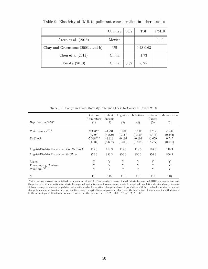
Table 9: Elasticity of IMR to pollutant concentration in other studies

Country SO2 TSP PM10

Arceo et al. (2015) Mexico 0.42

Chay and Greenstone (2003a and b) US 0.28-0.63

Chen et al.(2013) China 1.73

Tanaka (2010) China 0.82 0.95

Table 10: Changes in Infant Mortality Rate and Shocks by Causes of Death: 2SLS

Cardio- Infant Digestive Infectious External MalnutritionRespiratory Specific Causes

Dep. Var: ∆IMRC (1) (2) (3) (4) (5) (6)

PollExShockPCA 2.300** -0.291 0.207 0.197 1.512 -0.289(0.995) (4.220) (0.330) (0.369) (1.374) (0.342)

ExShock -5.536*** -4.414 -0.196 -0.196 -2.659 0.747(1.904) (8.687) (0.409) (0.819) (2.777) (0.691)

Angrist-Pischke F-statistic: PollExShock 118.3 118.3 118.3 118.3 118.3 118.3

Angrist-Pischke F-statistic: ExShock 856.3 856.3 856.3 856.3 856.3 856.3

Region Y Y Y Y Y YTime-varying Controls Y Y Y Y Y YPollEmplPCA Y Y Y Y Y Y

N 118 118 118 118 118 118

Notes: All regressions are weighted by population of age 0. Time-varying controls include start-of-the-period GDP per capita, start-of-the-period overall mortality rate, start-of-the-period agriculture employment share, start-of-the-period population density, change in shareof boys, change in share of population with middle school education, change in share of population with high school education or above,change in number of hospital beds per capita, change in agricultural employment share, and the interaction of year dummies with distanceto the nearest port. Standard errors are clustered at the province level. *** p<0.01, ** p<0.05, * p<0.1

50

Appendix not for Publication

A Event Study: the 2002 US Steel Safeguard Measures

In this appendix we perform a separate exercise aimed at answering the question: are exports

shocks generated by trade policy in the rest of the world large enough to affect local pollution

measures in China? We investigate the issue through a specific event, i.e., the US imposition of

safeguard tariffs on imports of steel products in March 2002 (and its removal in December 2003).

On June 28, 2000, the US Trade Representative (USTR) requested that the US International

Trade Commission (ITC) commence a Section 201 investigation on whether steel imports of 612

different 10-digit HS product categories were causing injury to the domestic industry. The USITC

investigation covered imports with a combined value of some $17 billion, more than half of total

US imports of steel in 2001. On October 22, 2001, the ITC announced its findings that 85% of the

imported products subject to investigation had caused injury to the domestic steel industry, and

in December 2001, the ITC announced its non-binding recommendation for safeguard tariffs and

quotas. On March 20, 2000, President George W. Bush announced the application of safeguard

tariffs and quotas on 272 different 10-digit HS product categories, which were significantly higher

than that recommended by the USITC Commissioners45 (Read, 2005; Bown, 2013). To retaliate

against the US safeguard measures and mitigate the associated diversionary effects, the EU im-

posed temporary safeguard measures on its steel imports on March 28, 2002 and introduced final

safeguard measures on September 29, 2002. According to the World Bank Temporary Trade Bar-

riers Database, 225 different 10-digit HS product categories were subject to investigation, among

which 53 were covered by safeguard tariffs. China also initiated its own safeguard measures on

May 20, 2002. On December 4, 2003, the US lifted all the safeguard tariffs and the EU and China

removed their measures in the same month. Figure A.1 summarizes the timeline of the 2002 steel

safeguards, with different colors indicating different stages which include investigation, provisional

measures, final measures and scheduled liberalization.

As documented by Read (2005), it is generally understood that tariffs were imposed for reasons

related to domestic political consideration and are unlikely to be related in their timing and

magnitude to events happening in China. This event is useful for our study because it pertains

an industry whose activity is highly polluting, like steel. According to the World Bank IPPS

data on emission intensity employed by Levinson (2009), SIC industry 331 and 332 are in the

top 10% industries by emissions of both SO2 and particulate matter.46 We exploit this event to

detect whether a temporary protection measure in the US that raised import tariffs on several

45185 products received a 30% tariff, 60 received a 15% tariff, 15 received a 13% tariff and 7 received a 8% tariffin the first year. In 19th March 2003, the tariffs for each of the categories stepped down to 24%, 12%, 10% and7%.

46Steel mills closures have been used in Pope (1989), Ransom and Pope (1995) and Pope (1996) to detect theeffect of particulate matter concentration on health outcomes.

51

steel products affected air quality relatively more in prefectures that produce more steel. We are

interested in the differential level of air quality in steel-producing prefectures relative to other

prefectures before and after the steel safeguards. We use the daily data on air pollution index

(API), an overall measure of ambient air quality. API data are obtained from the MEP of China.

The dataset records the API of major prefectures in China starting from June 5th, 2000. The

number of prefectures covered increases from 42 in the early sample period to 84 by the end of

our sample period. Over 2001 to 2005, the average API declined from 83 to 73.47The specification

we employ is the following:

APIit = βShareSteeli ×NoSGt + αi + φry + γrm + εit ,

where APIit is the Air Pollution Index in prefecture i on day t, ShareSteeli is equal to the share

of employment in steel sectors (in percentage)48 and the dummy NoSG is equal to 1 in the period

before the investigation or after the revocation of the safeguards. (The time window of the steel

safeguard corresponds to the days between 28/06/2001 and 04/12/2003.)49 αi is a prefecture

dummy which controls for the time-invariant prefecture-specific factors that affect the air quality.

φry is the region-year fixed effects which in effect capture the unobserved region-specific shocks that

have independent effects on API. γrm represents region-month fixed effects which account for the

region-specific seasonal factors that affect API. 50 Standard errors are clustered at the prefecture

level. The different specifications in Table A.1 employ different time windows and interact the

variable ShareSteeli with different policy time dummies: AfterSGt is equal to 1 in the period

after the termination of the safeguard policy and BeforeSGt is defined similarly.

Our findings indicate that before and after the period during which the policy was in place the

API was higher in steel-producing prefectures. The effect is not very large, but strongly significant.

Column (8) of Table A.1 extends the window to August 2005 and indicates that the API (which

averages 78.7) decreased by 2.53×0.8 = 2 points during the policy months in prefectures that had

the average share of steel employment relative to a prefecture that had no employment in steel.

Figure A.2 shows the estimates from the following specification

APIit =∑τ

λτShareSteeli + αi + φry + γrm + εit ,

47For the balanced panel of 42 prefectures, the average API declined from 86 to 73.48Employments under the code 32 and 34 of the CSIC 1994 classification, which pertain to steel and steel-related

products. Employment data is from the 2000 population census.49We find that exports from China to the US start declining during the investigation phase. This “investigation

effect”, originally analyzed theoretically and empirically by Staiger and Wolak (1994), was also detected in thesame context by Bown (2013).

50There are 8 regions: Northeast (Heilongjiang, Jilin and Liaoning), North Municipalities (Beijing and Tianjin),North Coast (Hebei and Shandong), Central Coast (Shanghai, Jiangsu and Zhejiang), South Coast (Guangdong,Fujian and Hainan), Central(Henan, Shanxi, Anhui, Jiangxi, Hubei and Hunan), Southwest (Guangxi, Chongqing,Sichuan, Guizhou, Yunnan and Tibet) and Northwest (Inner Mongolia, Shanxi, Gansu, Qinghai, Ningxia andXinjiang).

52

where λτ ’s reflect the conditional correlation between the API and steel employment share that

vary across quarters. Consistent with the findings in Table A.1, we find the API is lower during

the period with steel safeguards.

B Theoretical Derivation of Export Shocks

In this section we present a simple Ricardian model of trade and pollutant emissions that ra-

tionalizes our empirical specification. The set-up is a standard Eaton-Kortum style model (see

Eaton and Kortum, 2002) with multiple sectors as in Costinot et al. (2012) and fixed emission

intensities by sector. Consider a world economy that features multiple prefectures in China, in-

dexed by i = 1, ..., C, and multiple regions in the rest of the world (henceforth ROW), indexed by

i = C+1, ..., N , and K sectors, k = 1, ..., K. Each sector features multiple varieties, indexed by ω.

Preferences are described by a Cobb-Douglas upper-tier utility function (with consumption shares

βk) and a lower-tier CES utility function. Each sector is characterized by an emission intensity

γk which is equal to the ratio of emissions divided by the value of output and is assumed to be

fixed.51 There is only one factor of production, labor, and the production function for variety ω

of good k in region i takes the following linear form:

Qik (ω) = zik (ω)Lik(ω) ,

where Lik(ω) denotes the labor employed in region i to produce variety ω of good k. The associated

labor productivity is represented by zik(ω), and it is drawn from a Frechet distribution Fik (·), that

is:

Fik (z) = exp[−(z/zik)

−θ] for all z≥ 0 .

We assume that there is a large non-manufacturing sector that also employs only labor and that

determines the wage wi.52 Trade between regions is costly and τijk denotes the iceberg cost of

shipping good k from region i to j. We maintain the standard assumption that τijk ≥ 1 if j 6= i

and τiik = 1. Markets are assumed to be perfectly competitive, and each region imports from the

lowest cost supplier. The producer price for each variety ω is given by pik (ω) = wi/zik (ω). The

value output of sector k in region i is Yik =∑

ω pik (ω)Qik (ω) = wiLik.

51We assume fixed emission intensities not only because of simplicity, but mostly because we do not have access tomicro-data at the prefecture level that would allow us to test predictions regarding the effect of trade on productiontechniques. The assumption of fixed emission intensities is also made in Shapiro (2016).

52This is not an innocuous simplification, but it can be justified by the broad structural change happening inChina during this period. Rather than a real agricultural sector, this large outside sector should be rather seen asa representation of the large pool of subsistence rural workers that would later migrate to urban areas during the1990’s and 2000’s. In the rest of the derivation we omit the impact of this rural agricultural sector on emissionsand this assumption can be interpreted in two ways. The first is that this type of agriculture did not contributesignificantly to pollution. The second interpretation is that the production function in that sector exhibited verylow marginal product of labor due to the high ratio of population to land and therefore departure of a large shareof the workforce had little effect on output.

53

Following Eaton and Kortum (2002), the value of exports of good k from prefecture i in China

to region j in the ROW is determined by:

Xijk = λijkβkYj ,

where λijk denotes the share of expenditure on good k in region j that is allocated to the products

from prefecture i. This share λijk depends on production and transportation costs according to

the following expression:

λijk =(wiτijk/zik)

−θ∑Ni′=1(wi′τi′jk/zi′k)−θ

.

We can calculate the size of each sector in each region, as approximated by the employment in

the sector Lik, as follows:

wiLik =N∑j=1

Xijk =N∑j=1

λijkβkYj . (14)

Finally, total emissions are simply given by Pi =∑

k γkYik .

B.1 Changes in Transport Costs: Deriving Export Demand Shocks

The exogenous shocks in this model come from changes in iceberg costs {τiRk}, where i is a

prefecture in China and we denote by R the set of all other regions in the rest of the world. In the

empirical section we will interpret these changes in transport costs as coming from a decline in

tariffs faced by Chinese exporters. Hats over variables denotes log changes (x≡ d lnx). We assume

that all regions in China face the same export cost, i.e. the same tariff, and that this common

tariff is therefore declining by the same amount for all prefectures τiRk = τi′Rk = τRk. Moreover

we assume that internal trade costs remain unchanged, that is τii′k = 0. Total differentiation of

equation (14) gives

dYik = dXiRk =XiRk

XCRk

dXCRk , (15)

where dXCRk is the change in exports of good k from China to the ROW due to a change in trade

cost.53 More specifically,

53More specifically, equation (15) is derived as follows:

dλiRk = −θλiRkτRk

dτRk +θλiRk

∑i′∈C λi′Rk

τRkdτRk = −θ(1− λCRk)λiRk

dτRkτRk

, (16)

where C is the set of regions in China. In this derivation, it is key to impose the contemporaneous change in tariffsin the rest of the world to be the same for all regions in China. Analogously, the change in China’s share in the rest

54

dXCRk = XCRk × τRk (17)

Then, the total change in emissions is given by:

dPi =∑k

γkXiRk

XCRk

dXCRk . (18)

In our empirical work, our available measure of environmental quality is the change in emission

concentration in region i, Ci, where air pollutant levels are measured per cubic meter. Since

prefectures are different in size, the pollution concentration and and export shocks are related as

follows:

dCi ∝∑k

γkXiRk

XCRk

dXCRk

Li. (19)

where Li denotes the size of prefecture i.

Equation (19) sheds light on how external demand shocks at the national level lead to differ-

ential environmental impact across prefectures in China. In particular, we show that a prefecture

receives a larger pollution export shock if it specializes in dirty industries that experienced larger

declines in trade costs. The weighted average structure of export pollution shock resembles the

empirical approach in the literature on the local effects of trade (Autor et al., 2013; Topalova, 2010;

Kovak, 2013). However, it specifically reflects the pollution content embodied in the trade-cost

induced export growth, rather than overall export expansion.

C Data Appendix

C.1 Administration Division: Consistent Prefectures

Each prefecture is assigned a four-digit code in the censuses. The codes can change over years,

usually due to the urbanization of the rural prefectures (“Diqu”) to urban prefectures (“Shi”),

which does not necessarily mean re-demarcation. The changing boundary of prefectures is a threat

to the consistency of our defined local economies over time. To cope with the problem, we construct

a concordance mapping the counties in 1990, 2000 and 2010 to the prefectures where they belong in

2005. By construction, we have consistent 340 prefectures over years. The municipalities Beijing,

Chongqing, Shanghai and Tianjin are treated as prefectures in this paper.

of the world imports is dλCRk = −θ(1− λCRk)λCRkdτRk

τRkand we can combine dλCRkwith equation (16) to find:

dλiRk =XiRk

XCRkdλCRk .

Simple manipulation yields equation (15).

55

C.2 Industrial Classifications

Our dataset is complied from multiple sources which adopt different industrial classifications. We

map the data on employment share, emission intensities, exports, tariffs, and so on to consistent

3-digit CSIC codes. The details are provided as follows. (1) CSIC employed by our data sources

has three versions, CSIC1984, CSIC1994 and CISC2002. We firstly build the concordances which

map 4-digit CSIC codes of different versions to consistent 3-digit CSIC codes. (2) To convert the

ISIC data to CSIC, we employ the concordance built by Dean and Lovely (2010) which cross-

matches the four-digit CSIC2002 and ISIC Rev.3. (3) For the SIC data, we firstly concord it to

ISIC Rev.3 using the concordance provided by the United Nations Statistics Division, and then

map it to CSIC2002.

C.3 Computation of Three-Digit Industry Emission Intensity

Pollution intensity for each pollutant p, of a 3-digit CSIC industry k, is imputed following these

steps: (i) using industry output as weight,54 we aggregate the 3-digit IPPS data γp,IPPSk to 2-

digit CSIC level, i.e., γp,IPPSK where K is a 2-digit CSIC sector; (ii) for each 3-digit industry, we

calculate the ratio of its pollution intensity to the corresponding 2-digit sector pollution intensity,

i.e., rp,IPPk = γp,IPPSk /γp,IPPSK ; (iii) we impute pollution intensity for each 3-digit industry according

to γp,MEPk = rp,IPPk × γp,MEP

K . Therefore, while the level of industry pollution intensity is aligned

with the MEP data, the within sector heterogeneity retains the feature of the IPPS data. To

account for changing industry pollution intensity over time, we use the 1996 and 2006 data from

MEP and construct measures for each decade t. Pollution intensity γp,MEPkt is employed to build

pollution export shocks as is discussed in Section 3.

C.4 Death Records in Population Census

According to the enumeration form instructions of the China population censuses, both birth

and death are registered at the household level, where the newborn and the deceased belong to.

Therefore, in principle, the census data accurately record the number of births and deaths within

a geographic unit. To evaluate the potential measurement errors introduced by migration, let’s

consider the following scenarios. First, a mother gave birth in a village, then migrated to a city

and lived in a factory dormitory. Her newborn was left behind and taken care by grandparents in

the rural area. If her baby unfortunately died, the death will be registered in the grandparents’

household, but not in the factory dormitory. In this case, infant mortality is accurately measured

in both city and rural areas. Second, a migrant female worker gave birth in a city, and sent her

baby to rural village. Her baby unfortunately died because of earlier exposure to air pollution in

the city. In this case, the birth is counted in the city and the death is counted in the rural area.

54Data on output by industry is from the Chinese Industrial Annual Survey.

56

As a result, our estimate understate the true effect of pollution on IMR. Nevertheless, we consider

that the second scenario is less likely in the Chinese context due to restrictions on migrant workers’

access to public health service in cities.

C.5 Relative Employment Ratio Employed in Figure 1

To construct the employment ratio employed in Figure 1, we first group industries into Clean (C)

and Dirty (D) groups, according to whether the sectoral value of SO2 emission intensity is above

or below the median. The clean industry group has an average SO2 emission intensity of 1.46

pounds per thousand dollar value output. In contrast, the emission intensity for dirty group is

16.2 pounds per thousand dollar value output. Then, we group industries into HighShock (H),

MediumShock (M) and LowShock (L) groups, according to whether the industry lies in the upper,

middle or bottom tertile of dollar export growth per worker during the period 2000-10. We find

that HighShock industries experienced export shock of 168.1 dollars per worker on average. The

corresponding values of MediumShock and LowShock groups are 17.35 and 3.77, respectively.

Using the 2000 census data, for each prefecture, we calculate its employment in industries that are

Clean and experienced HighShock (EmpShare(CH)), and similarly values for EmpShare(DH),

EmpShare(CL) and EmpShare(DL). Then, we construct the relative employment ratio of high-

export-growth industries as follows:

EmpSharei(DH)

EmpSharei(CH) + EmpSharei(DH).

Analogously, the relative employment ratio of low-export-growth industries is:

EmpSharei(DL)

EmpSharei(CL) + EmpSharei(DL).

C.6 Prefecture Level Data on Wind Direction

The data on wind direction is collected from NOAA Integrated Surface Global Hourly Data. We

collapse the hourly data to the daily level and calculate the average wind direction for each weather

station-day observation using the “unit-vector” average method according to NOAA.55 The wind

direction is categorized into 37 groups, i.e., d ∈ {0, π36, ..., 35π

36, No Wind}. We drop the weather

stations with more than 40% of the daily observations within a decade are missing. There are 544

and 394 weather stations in our samples for the decade 1990-2000 and 2000-2010, respectively.

We impute the data on wind direction to each prefecture using the data from its nearest

weather station.56 For each prefecture, we calculate the share of days that the wind direction is d

55More details can be found in http://www.ndbc.noaa.gov/wndav.shtml.56The nearest weather station is identified as the one with the shortest distance to the centroid of a prefecture.

We obtain similar results using the data from the first and second most nearest weather stations.

57

for each decade, i.e., 1990-2000 and 2000-2010. It is denoted by sit,d.

C.7 Other Demographic and Socioeconomic Data

We collected other demographic and socioeconomic variables at the prefecture level, including

GDP per capita, provision of medical care, sex ratio of the newborns, share of population with

different educational attainments, share of agricultural employment, and population density from

various provincial statistical yearbooks and population censuses. The distance to the nearest port

for each prefecture is calculated using the information from the World Port Index. In addition, for

the period of 2000 to 2010, we obtain the prefecture-level information on output by 3-digit CSIC

industry, fossil fuel energy production, and production shares of state-owned enterprises (SOE)

and foreign firms from Chinese Industrial Annual Survey.57 We also obtain the transaction-level

export data from China’s General Administration of Customs to construct actual dollar value of

export and pollution content of export at the prefecture level for 2000 and 2010.

C.8 Employment Weighted and Wind Direction Weighted Neighbor-

ing Export Pollution Shocks

We identify the set of prefectures sharing a border with each prefecture i, and denote it by

Neighbori. The employment weighted neighboring export shock is defined as follows:

ExShockNi,t =∑

n∈Neighbori

ψintExShockpnt ,

where ψint = Ln,t−1∑n′∈Neighbori

Ln′,t−1denotes the employment weight of prefecture n among all the

neighboring prefectures of i.

The wind direction weighted neighboring export pollution shock is constructed as follows

WindPollExShockp,Ni,t =∑

d∈{0, π36,..., 35π

36,NW}

∑n∈Neighbori

πint,dPollExShockpnt .

The neighboring prefecture n’s export pollution shock is weighted by

πint,d =snt,dwin,d∑

d

∑r snt,dwin,d

,

where snt,d denotes the share of days in which the wind direction is d in neighboring prefecture

n and decade t. win,d captures the weight of different wind directions. It is determined by the

57The data set includes all the state owned firms and non-state firms with revenue above 5 million RMB (ap-proximately 800 thousand US dollar).

58

relative position between i and n and the wind direction in n, and it is constructed as follows:

win,d =

{12[1 + cos(θin,d)] if d ∈ {0, π

36, ..., 35π

36}

0 if d = No Wind,

where θin,d denotes the absolute value of the angle between neighboring prefecture n’s angular

position and its wind direction d. The example in Figure A.4 illustrates how θin,d is calculated.

The green triangle represents a prefecture, who has three neighboring prefectures (n = 1,2 and

3) represented by blue circles. The neighboring prefectures are located in the Northwest, South

and East. (Their angular position to i are 3π/4, 3π/2 and 0, respectively.) Suppose the wind

directions in the three neighboring prefectures are π/4, 0 and π/3, respectively. Then the angles

between their angular position and wind direction are θ1,π/4 = π/2, θ2,0 = π/2 and θ3,π/3 = π/3,

respectively. Note that win,d = 1 if prefecture i is in the downwind position of n, i.e., θin,d = 0,

and win,d = 0 if prefecture i is in the upwind position of n, i.e., θin,d = π. This weighting scheme

is intuitive. Prefecture i receives more cross-border pollution from prefecture n if i is located

downwind of n more often, i.e., snt,dwin,d is larger.

C.9 Input-Output Tables

To construct the alternative export shocks as described in Section 4.3.3, we use the 1997 and

2007 input-output (IO) tables published by National Bureau of Statistics China. The 1997 IO

table contains information of input-output relationships among 124 industries, 70 of which belong

to manufacturing sector. The 2007 IO table contains information of input-output relationships

among 135 industries, 80 of which belong to manufacturing sector. We aggregate and match our

trade, employment and pollution intensity data to the industries in the IO tables.

D Quality Assessment of the Chinese Data Pollution and

Mortality

In this section, we address the concern that official reports from the Chinese government may not

be fully reliable due to the desire to misreport pollution and mortality.

D.1 Data Quality of Air Pollution: Comparison of Official Data and

US Embassy Data

Since 2009, the US Embassy started to monitor and report the hourly concentration of PM2.5,

the particulate matters up to 2.5 micrometers in size, in five major cities in China, i.e., Beijing,

Chengdu, Guangzhou, Shanghai and Shenyang. The data are collected independently of Chinese

59

government agencies, and hence provide a benchmark to check the validity of the official pollution

data. As discussed earlier, environmental protection was unlikely to be a major factor determining

a politician’s career trajectory in the past, so if the manipulation of the official pollution data

existed, it is more likely to have occurred in the later period. Therefore, we believe the comparison

is informative, although it is restricted to the later years.

Daily Average of Air Quality Index (AQI)

MEP publishes AQI and the main pollutant daily for major cities in China. According to MEP,

the AQI and the main pollutant are derived following the steps: (1) convert the pollution read-

ings to IAQIp for each pollution p; (2) construct the overall AQI using the formula AQI =

max{IAQI1, IAQI2, ..., IAQIP}; (3) the main pollutant is p if IAQIp = max{IAQI1, IAQI2, ..., IAQIP}.The information of individual pollutant index IAQIp is not public available. However, we know

that AQI = IAQIPM2.5 conditional on the main pollutant being PM2.5.

We obtain the daily data from MEP for 2014. The hourly data from US Embassy is aggregated

to daily data, and converted to IAQIPM2.5 using the conversion table provided by MEP. The

summary statistics of the two data series are presented in Table A.3. We find that, conditional

on that the main pollutant being PM2.5, the correlation of the two series is very high, ranging

from 0.94 for Chengdu to 0.97 for Shanghai. The average IAQIPM2.5 of MEP data is generally

lower than the US embassy data, with largest discrepancy observed for Beijing. The discrepancy

is likely be due to the different locations where the data is collected. In each city, the US embassy

readings are collected from only one monitor located in a populous area, while the MEP readings

are collected from multiple locations including suburban areas.

Annual Average of PM2.5 (PM10) Concentration

The cities in China started to monitor PM2.5 in 2013. Until then, only the concentration level of

PM10, the particulate matters up to 10 micrometers in size, was reported. As the PM2.5 belongs

to the PM10, the concentration level of the former should always be smaller than the latter. It

is taken as strong evidence for data manipulation if we detect the concentration level of PM10

reported by MEP is smaller than that of PM2.5 reported by US Embassy. As is shown in Table

A.4, the official data of PM2.5 track the US Embassy data closely in 2013. In addition, we fail to

find any case such that the concentration level of PM10 reported by MEP is smaller than that of

PM2.5 reported by US Embassy.

D.2 Data Quality of IMR: Comparison of Cohort Size across Censuses

Infant mortality rate is measured with error if either number of births or number of deaths is

misreported. One may concern that due to the One Child Policy, households may have incentives to

60

underreport live births or over-report infant mortality to hide unsanctioned births. To investigate

this possibility, we compare the population size of a newborn cohort across census years. In

particular, we predict the cohort size of Age 0 ten years later, Pop0,i,t+10, using the information of

mortality rate of age groups of 1-4 and 5-10, as follows

Pop0,i,t+10 ≈ (Bi,t −D0,i,t)(1−D1−4,i,t

Pop1−4,i,t

)4(1− D5−10,i,t

Pop5−10,i,t

)5 ,

where Bi,t is the number of births of prefecture i in census year t, Da,i,t and Popa,i,t denote

respectively the number of deaths and population of age group a in prefecture i and census year t.

In principle, without inter-region migration, the predicted population size of Age 10 in census year

t+10, Pop0,i,t+10, should closely track the actual population size if the data on number of births and

deaths are free of measurement error. However, if either Bi,t is prevalently underreported (over-

reported) or D0,i,t is over-reported (underreported), one should expect the predicted population

size of Age 10 to be always smaller (larger) than the actual data.58

Figure A.5 plots the log of predicted Age 10 population Pop0,i,2000+10 (derived from the 2000

census), against the log of actual Age 10 population Pop10,i,2010 (obtained from the 2010 census).59

The points are closely cluster along the 45 degree line, suggesting the birth and death statistics are

not systematically misreported. The coefficient of correlation between the predicted and actual

log Age 10 population is as high as 0.984. In addition, we find that the prefectures that lies

significantly below the 45 degree line are the ones receiving large net inflows of immigrants. As a

result, the actual population size is larger than the predicted population size.

E Employment Share and Export Share

In this section, we use data in 2000 and investigate the correlation between a prefecture’s share in

national export and its employment share. Specifically, we estimate the following regression60

XiRk

XCRk

= αLikLCk

+ εik .

The estimated coefficient of α is 0.965 with robust standard error 0.046. The null hypothesis

H0 : α = 1 cannot be rejected. As is discussed below, when α = 1 and under certain condi-

tions, the discrepancy between the export share and the employment share only leads to classical

measurement error and results in attenuation bias.

58As it is more difficult to hide a ten-year-old than an infant, we consider that the actual population size of Age10 in census year t+ 10 is subject to less misreporting.

59The findings are similar when comparing the 1990 and 2000 censuses (available on request).60The export share is derived from 2000 data of the Chinese Industrial Annual Survey. Note that the survey

does not cover private firms with annual revenue below 5 million RMB. As a result, the data on export share arealso subject to measurement errors.

61

Consider the following (simplified) model:

yi = β0 + β1xi + ui ,

where xi =∑

k πik∆XCRk and πik = XiRk/XCRk. Due to the data limitation, we cannot observe

πik directly and use πik = Lik/LCk as a proxy instead. We have established that, from the data,

πik = πik + εik. Hence,

yi = β0 + β1xi + (ui + β1ei) ,

where xi =∑k

πik∆XCRk =∑k

πik∆XCRk︸ ︷︷ ︸xi

−∑k

εik∆XCRk︸ ︷︷ ︸ei

= xi − ei .

In the following discussion, we make a simplifying assumption that

limN→∞

1

N

∑i

uiei = limN→∞

1

N

∑k

∆XCRk

∑i

εikui = 0 ,

i.e., in the limit the measurement error is uncorrelated with the other unobserved determinants.

Then, it is straightforward to show that the approximation of XiRk/XCRk by Lik/LCk only leads

to classical measurement error if

limN→∞

1

N

∑i

xiei = limN→∞

1

N

∑i

(∑k

πik∆XCRk

∑k

εik∆XCRk

)= 0 .

A sufficient condition for limN→∞1N

(∑

i xiei) = 0 is limN→∞1N

∑i πi,kεi,k′ = 0 ∀k, k′. That is, in

the limit the measurement error is uncorrelated with a prefecture’s export share.

F Additional Results

F.1 Multicollinearity Problem and Monte Carlo Simulation

The correlation between PollExShock and ExShock is 0.74, leading to a concern about mul-

ticollinearity. In the following, we conduct Monte Carlo simulations to assess the sensitivity of

our results to the potential multicollinearity problem. In particular, we consider the following

reduced-form model:

yit = β1x1,it + β2x2,it + εit, (20)

where x1 and x2 are the actual data corresponding to PollExpShock and ExShock. The error

term ε is drawn from the normal distribution N(0, σ2), where σ is the standard deviation of the

residuals from the baseline model (i.e., regression in column (7) of Table 3). We consider two

cases with different values of β1 and β2. For each case, we simulate 500 datasets. By design, the

simulated data has the same number of observations and the same correlation of the two variables

62

of interest as in the actual data.

Case I: β1 = 2.5 and β2 = 0. We estimate equation (20) using the 500 simulated datasets. Column

(1) of Table A.5 reports the average and the standard deviation of the estimates of β1 and β2.

We find that on average, both estimates are very close to their true values. Column (2) drops x2

from regression. The average of β1 barely changes since β2 = 0. In column (3), we estimate the

misspecified model with x1 omitted, and find that β1 is severely biased. This finding echoes the

results in column (3) of Table 3 in the main text, suggesting that the estimate of export income

effect is severely biased without controlling for the pollution effect.

Case II: β1 = 2.5 and β2 = −1. Multicollinearity leads to noisy estimates. If it is a valid concern,

we may obtain statistically insignificant coefficients even if the true effects are non-zero. (In

our context, one may worry that the insignificant coefficient on ExShock is a result from the

multicollinearity problem.) To alleviate the concern, we simulate datasets by setting β2 = −1.

Columns (4) estimates equation (20). Again, we find that both estimates are very close to their

true value. More importantly, both estimates are statistically significant at the 1% level. We

take this finding as suggestive evidence that our identification is unlikely to be hindered by the

correlation between the two variables.

The main takeaways from this exercise are twofold. First, it is exactly because of the correla-

tion between PollExpShock and ExShock, the estimated export income effect has a wrong sign

in a misspecified model without accounting for the pollution effect. Second, despite the high

correlation, there is sufficient statistical power to identify their independent effects.61

F.2 Rotemberg Weights

In this section, we compute the Rotemberg weights of export pollution shocks and export shocks

with controls, aggregated across time periods.62 The industry-specific Rotemberg weights capture

the degree of sensitivity to misspecification when the exogeneity assumption of initial industry

composition fails. In particular, the 2SLS estimates are more sensitive to the bias introduced by

an industry with a larger Rotemberg weight.(Goldsmith-Pinkham et al., 2018) Table A.7 reports

the five industries with the highest Rotemberg weights for PollExShockTSP and ExShock, re-

spectively. For pollution export shock, these industries are graphite and carbon products, leather

61Autor et al. (2018) employ gender-specific components of import supply shocks to investigate the impacts ofshifts in relative earnings of young men versus young women on marriage, fertility and children’s living circumstance.Similar to our case, despite the high correlation between their by-gender measures (0.80), they are able to distinguishthe independent effects.

62In this exercise, we adopt the measure PollExShockTSP . Therefore, the industry-level trade shock for export

pollution shock is γTSPkt∆XCRkt

Lck,t−1. The industry-level trade shock for export shock is ∆XCRkt

Lck,t−1. Different from the cases

discussed in Goldsmith-Pinkham et al. (2018), we have two endogenous variables. When we construct Rotemberg

weights for PollExShockTSP , we include ExShock as a control. Similarly, when we construct Rotemberg weights

for ExShock, we include PollExShockTSP as a control. We also in include all the controls listed in column (7) ofTable 3.

63

products, games and toys, brick and clay and related products, and refractory products.63 The

top five industries account for 29.5% of the positive weights in the Bartik estimator, which is

lower than the cases studied in Goldsmith-Pinkham et al. (2018). For export shock, the top five

industries are games and toys, electronic components, other plastic products, metal products for

daily uses, and leather products. The sum of the Rotemberg weights of these industries amounts

to 43.8% of the positive weights in the Bartik estimator.

One may worry that our baseline estimates are confounded by the prefecture-specific pre-

trends that are correlated with initial shares of these industries. To allay the concern, we relate

the trends of IMR to initial shares of these potentially influential industries by estimating the

following regression:

∆IMRit = β0 + βτEmpShareki,90 + γrt + εit,

where EmpShareki,90 denotes industry k′s share in total employment of prefecture i in 1990 (in

percentage), and γrt is the region×year fixed effects.64 We allow the coefficients βτ to vary over

time, where τ ∈ {1990, 2000, 2010}. We then convert the changes in IMR to levels, and the levels

in 1982 are normalized to be 0. Standard errors are constructed using the delta method. Figure

A.6 presents the findings for the industries listed in Table A.7. Across the industries, there are

no obvious pre-trends in the pre-periods, i.e., 1982-1990. For all industries, we observe stark

changes during 2000-2010, when China experienced a rapid export expansion. We consider these

findings as supporting evidence that our baseline estimates are unlikely to be severely biased by

confounding trends.

F.3 Dropping One Sector or Two Sectors at a Time

To assess the sensitivity of our baseline results to any specific industries, we reconstruct the trade

shocks and corresponding instruments but leave out one or two 2-digit CSIC sectors at a time.65

We repeat the regression in column (7) of Table 3 using these alternative measures of trade shocks.

Columns (1) and (2) of Table A.8 report the range of the estimates for the case where we drop

one sector at a time. The estimated effects of pollution export shock range narrowly from 2.098

and 2.613, and remain significant at the 1% level. Columns (3) and (4) show the ranges when we

leave out two sectors at a time. The lower- and upper-bounds of the estimates are statistically

indifferent. These findings alleviate the concerns that the baseline estimates are (i) driven by

certain polluting industries, and (ii) confounded due to the endogeneity associated with initial

employment share of several influential sectors (Goldsmith-Pinkham et al., 2018).

63The list include three industries with pollution intensities at the top 5 percentile. These industries are graphiteand carbon products, brick and clay and related products, and refractory products.

64The results remain similar when we use 2000 employment share.65There are 38 2-digit CSIC sectors.

64

F.4 Balance Test of Industry-Level Shocks

The Bartik-style instrument can be generally formulated as∑

k siktgkt, where gkt denotes the shock

experienced by industry k and period t and sikt measures the exposure of location i to the shock.

In our context, gkt represents (i) the export demand shock in dollar value captured by ∆XCRktLck,t−1

, or

(ii) the associated pollution shock γpkt∆XCRktLck,t−1

.66 The exposure to each shock is captured by initial

employment share of the industry in local economy, i.e.,Lik,t−1

Li,t−1. As is discussed in Borusyak et

al. (2018), the validity of the instrument relies on the assumption that conditional on industry

controls,∑

k

∑t sktgktφkt

p−→ 0, where skt = E(sikt) measures the expected exposure to industry k

in period t and φkt = E(siktεi)/E(sikt) is an exposure-weighted expectation of untreated potential

outcomes. Put in other words, the identification relies on the assumption that, weighted by

skt and conditional on industry controls, the correlation between industry-level shocks gkt and

unobservables φkt approaches zero in large sample.

To substantiate this assumption, we follow Borusyak et al. (2018) and examine the random-

ness of the industry level shocks by testing the shock balance with respect to various regional

characteristics. This exercise also guides the choice of location-level controls. The results are pre-

sented in Table A.9. Each row reports the coefficients from regressing industry-specific average of

a prefecture characteristics (residualized by region-period fixed effects) on pollution export shock,

export shock, and period fixed effects. Standard errors are clustered by CSIC codes, regressions

are weighted by average industry exposure, and coefficients are multiplied by 100 for readability.

We find that conditional on export shock, the pollution-export shocks are statistically uncorre-

lated with all the prefecture characteristics expect PollEmpl.67 For example, the third row implies

that pollution export shocks are not concentrated in locations that experienced relatively faster

increase in IMR in the preceding decade. These findings suggest that conditional on export shock

and PollEmpl, pollution-export shock could be as good as randomly assigned across industries.

For export shock, there are more coefficients are are statistically different from zero, albeit they

are small in magnitude. For example, the fourth row suggests that export shocks tend to be larger

in prefectures that were initially richer. Therefore, in most of location-level regressions, we control

for these location-specific characteristics.

F.5 Statistical Inference and Industry-Level Regression

In the baseline analysis, we cluster standard errors at the province level, which allows for arbitrary

within-province correlation and assumes that there is no cross-province correlation in the error

terms. This assumption may be too strong if there is substantial cross-province correlation that is

66In this exercise, we consider TSP pollution shock. Results remain similar for SO2 or NO2 pollution shock.67As shown in the first row, it is unsurprising that pollution export shocks tend to be larger in prefectures with a

higher share of dirty industries, which the need of controlling for PollEmploymentit−1 in (5) for the prefecture-levelregression analysis.

65

due to the similarity of industry structure across prefectures that are not geographically proximate

(Adao et al. 2018). As a robustness check, we follow Borusyak et al. (2018) and conduct the

analogous analysis at the industry level, which overcomes such concerns about statistical inference

of shift-share research designs.68 The results are reported in Table A.10. The point estimates from

the industry-level regression is equivalent to the prefecture-level regression. More importantly,

the two approaches provide similar statistically inference – the effects of PollExShock remains

statistically significant at the 1% level. We take the above check as reassuring that the spatial

correlation of residuals due to similar industrial composition is unlikely to bias the standard errors

in our baseline analysis.

F.6 Initial Size of the Agricultural Sector/Tradable Sector

One may concern that there could be differential pre-determined trends in IMR in the initially

agricultural regions. Our baseline specification controls for the initial agricultural employment

share, which partly accounts for the pre-trends and/or other omitted variables that are correlated

with the initial size of the agricultural sector. Column (1) of Table A.11 addresses this concern

in a more non-parametric way by including quintile dummy variables for the initial agricultural

employment share. The results remain stable. This finding, together with a variety of extensions

and sensitivity checks regarding pre-trends discussed above, suggests that our baseline findings

are unlikely to be driven by initial size of the agricultural sector.

For our baseline measures, the shocks to the non-traded sectors are set to zero. Therefore, a

part of variation arises from the importance of tradable sector for local employment. We take two

approaches to to alleviate the concern that our baseline findings are confounded by the initial size

of the tradable sector. First, in column (2) of Table A.11, we control for quintile dummy variables

for the initial employment share of the tradable sector. The estimates resembles the baseline

findings. Second, in column (3), we reconstruct the Bartik measures using the employment shares

within the traded sector as weights, and find consistent results.

68For the industry-level analysis, we first residualize the prefecture-level IMR and treatments (i.e., PollExShockand ExShock) by projecting these variables on the controls listed in column (7) of Table 3. To obtain the industrylevel IMR, PollExShock and ExShock, we then aggregate the residuals to the industry level based on witsikt

1N

∑Ni=1 witsikt

,

where wit represents the weights for prefecture-level regression, i.e., population of age 0 at the start-of-period. For

the industry-level regression, the instruments for the treatments are γpt∆XCRkt

Lck,t−1and ∆XCRkt

Lck,t−1. In this exercise, we

consider TSP pollution shock. Results remain similar for SO2 or NO2 pollution shock. As a related note, we mayconstruct industry-level measures using the weighting scheme sikt

1N

∑Ni=1 sikt

, and the regression result is equivalent to

that of the unweighted prefecture-level regression. The results as followed remain similar.

66

F.7 Reduction in Trade Policy Uncertainty

China was granted permanent normal trade relation (PNTR) status by the US upon its accession

to the WTO, which reduces the trade policy uncertainty faced by Chinese exporters. Existing

studies find that this exogenous shock has an significant impact on China’s labor market (Erten

and Leight, 2019; Facchini et al., 2019). In our baseline analysis, we adopt changes in tariffs

faced by Chinese exporters instead of the reduction of trade policy uncertainty as the exogenous

export demand shocks for two reasons. First, the sample period of our paper spans from 1992

to 2010. While the PNTR granted by the US provides useful exogenous variation for the second

decade (2000-2010), it lacks power to explain the export expansion in the first decade (1992-2000).

Second, the external tariff changes allows us to isolate the export demand shocks from the ROW

instead from the US alone.69

If we restrict our analysis to the 2000s, the goal of isolating the exogenous variation in exports

can be achieved by exploiting different exogenous demand shifters – either they come from actual

tariff changes or uncertainty in trade policies. In this appendix, we use the NTR tariff gap to

generate exogenous export demand shocks. If both the external tariff and the NTR gap are valid

instruments for export flows, our results should be robust to different IV approaches. We use

the NTR gap and corroborate the baseline findings by two steps. First, we compare the power

of the external tariff and the NTR gap in explaining export flows at the industry level in Table

A.12. Second, we demonstrate that our results are robust to alternative instrument formulations

in Table A.13.

Column (1) of Table A.12 estimates the following model:

∆ lnExportkt = α + θ∆ ln(1 + ExTariffkt) + εkt, (21)

where ∆ lnExportkt and ∆ ln(1 + ExTariffkt) denote the changes in export and external tariffs

(in logs) of industry k during the period 2000 to 2010. The estimated coefficient implies a trade

elasticity of 7.8, which resembles the baseline estimate in Figure 3 of the main text. We then

follow Pierce and Schott (2016) and Handley and Nuno (2016), and relate the export flows to the

NTR gap (a proxy for the reduction in trade policy uncertainty):

lnExportkt = ψk + δt + γ1(t = 2010)×NTR Gapk + εkt (22)

where NTR Gapk = ln(1 + NonNTR Tariffk) − ln(1 + NTR Tariffk).70 ψk and δt denote

industry and year fixed effects, respectively. The coefficient γ captures the effect of the reduction

in trade policy uncertainty on export growth. For the ease of comparison with model (21), we

69The US share in Chinese total export is 20.9% in 2000.70The data on NTR and non-NTR tariffs are obtained from Pierce and Schott (2016). We aggregate the the

HS 8-digit product level tariffs to the 4-digit ISIC industries using the US imports from China in 2000 as weights.(The data on US imports at the 8-digit HS level are obtained from the US Census Bureau.)

67

estimate equation (22) using the first-difference model:

∆ lnExportkt = δ + γNTR Gapk + εkt. (23)

Consistent with findings in the existing literature, industries with a higher NTR gap experienced

a faster export growth during the decade. More importantly, the R-squared from model (3) is

slightly lower than that of model (1). The finding implies that NTR gap does not outperform

external tariffs in terms of its strength as an instrument. In column (3), we conduct a horse-race

between the external tariff and NTR gap. The estimated coefficients remain statistically similar

to those in columns (1) and (2). In terms of magnitude, we find that a standard deviation decline

in external tariff induces export to grow by 0.35 log point, while a standard deviation increase in

NTR gap raises export by 0.26 log point.

Having established the link between export and NTR gap, we construct alternative instruments

as equations (8) and (9) in the main text, but replace ∆Xkt by the changes in exports predicted

by the reduction in trade policy uncertainty. More specifically, we obtain the exponential of the

fitted value from equation (22), Xkt = exp(ψk + δt + γ1(t = 2010) × NTR Gapk) and derive the

decadal difference ∆Xkt.

In Table A.13, we restrict the analysis to the 2000s and check robustness with respect to different

ways of formulate instruments. Column (1) adopts the baseline IVs constructed from external

tariffs (as discussed in section 3.2), while column (2) uses the alternative IVs constructed from

the NTR gap. Reassuring, we find the estimates are statistically similar. In column (3), we adopt

atheoretical instruments as follows:

PollExShockp

it =∑k

γpktLik,t−1

Li,t−1

NTR Gapk and ExShockit =∑k

Lik,t−1

Li,t−1

NTR Gapk.

Again, the IV estimates remain robust while the first stage results are weaker.

F.8 Changes in Other Trade Policies

In this appendix, we assess the likelihood that our estimates are severely biased due the omission

of other trade policy shocks associated with China’s accession to the WTO.

Direct trading right. As is shown in Bai et al. (2017), the removal of the restrictions on direct

export promoted trade. It is important to note that before 2000, direct trading rights were granted

to firms based on whether registered capital, revenue, net assets, and exports exceeded threshold

levels. Such restrictions were gradually relaxed over 2000-2004. However, there is little cross-

industry variation in the intensity of these restrictions and the timing of their removal.71 Therefore,

71Mechanical and Electronic Products is the only sector that was subject to a lower threshold. For more details,please refer to the appendix of Bai et al. (2017).

68

this policy experiment is not ideal for our current approach to identify the effects of export shocks.

(Recall that our identification strategy relies on the cross-industry variation in export expansion.)

In fact, to the extent that the removal of direct export right affects industries similarly, its pollution

effect on mortality and pollution will be captured by coefficients on PollEmpl. (See equation (5)

in the main text.)72 As is discussed in appendix F.3, our results remain stable when the sector

“Mechanical and Electronic Products” is dropped from the analysis.

Export licence. A related trade barrier is export licence, which was imposed on a set of

products in the pre-WTO period. According to the 2001 WTO report, 216 6-digit HS products

were subject export licence. For the purpose of our analysis, we aggregate the product-level

information and derive the coverage ratio of export license at the 4-digit industry level. In columns

(4) and (5) of Table A.12, we investigate whether the export grows faster in industries that were

more constrained by export license requirement in the pre-WTO period. The estimated coefficient

is positive, but statistically insignificant. Moreover, the R-squared in column (4) is much smaller

than those in columns (1) and (2). Given these findings, we decided not to purse an IV approach

based on the export restrictions. Moreover, the correlation of coverage ratio of export license and

∆ ln(1 + ExTariffkt−1) is -0.08 and statistically insignificant. Therefore, our baseline results are

unlikely to be biased by such export restrictions.

Quota removal under the Multi-fiber Agreement (MFA). The MFA only have impacts

on the textile sector, although there is substantial variation in changes in quota at the product

level within the sector. Due to the data constraint, we have to construct the pollution and export

shocks at the industry level, but there are only 11 industries in the textile sector.73 Moreover,

the variation in pollution intensity within the textile sector is smaller than the variation across all

industries.74 Therefore, at the prefecture level, the MFA does not provide us enough statistical

power to distinguish pollution effect from the income effect induced by export demand shocks. We

show in Appendix F.2 that our results remain stable when the textile sector is dropped from the

analysis. This finding alleviates the concern that due to the MFA, the textile sector is influential

and drive our findings.

FDI liberalization. To alleviate the concern about the confounding effects from the con-

current FDI liberalization, we collect information on China’s FDI regulations from the Catalogue

for the Guidance of Foreign Investment Industries. We compare the last version before 2000 (i.e.,

1997 version) and the last version before 2010 (i.e., 2007 version). In the Catalogue, products were

classified into four categories: (i) products where FDI was supported, (ii) products where FDI was

permitted (not listed in the Catalogue), (iii) products where FDI was restricted, and (iv) products

72If the change in export per worker (∆Xkt/Lk,t−1) induced by the removal of the restrictions on direct exportis similar across industries, PollExShock boils down PollEmpl multiplied by a constant term.

73This constrain stems from the fact that our employment data are derived from the China Population Censuses,which is at the 3-digit CSIC level.

74For example, the coefficient of variation of emission intensity of TSP within the textile sector is 1.41. Thecoefficient of variation across all industries is 2.89.

69

where FDI was prohibited. We consider the FDI for a given product is liberalized if it was moved

from the “restricted” or “prohibited” category to the “encouraged” or “permitted” category in

2007. Then, we aggregate the policy changes to the industry level. Specifically, FDILiberalizedk

is an indicator variable equals to one if there exists a liberalized product in industry k, and zero

otherwise.75 Column (6) of Table A.12 shows a positive but statistical insignificant effect of FDI

liberalization on export growth. The R-squard is much lower compared to columns (1) and (2).

Moreover, the correlation between FDILiberalizedk and ∆ ln(1 +ExTariffkt) is -0.1 and statis-

tically insignificant. Column (7) finds that estimated effects of external tariff and NTR gap are

insensitive to the control of FDI liberalization.

We further assess the potential confounding effects of FDI by constructing pollution FDI shock

and dollar value FDI shock at the prefecture level:

PollFDIShockpit =∑k

γpktLik,t−1

Li,t−1

∆FDIktLk,t−1

and FDIShockit =∑k

Lik,t−1

Li,t−1

∆FDIktLk,t−1

,

where ∆FDIkt is the change in FDI stock of industry k during the period 2000 to 2007.76 Analo-

gous to pollution export shock, PollFDIShock captures the pollution content of the FDI inflows.

Column (6) of Table A.11 reports the robustness check with FDI shocks as controls. Pollution

FDI shock tends to raise IMR, but the estimate is statistical insignificant. More importantly, the

estimated effects of export shocks remain statistically similar to our baseline findings.

F.9 Robustness Checks: Effect of Export Shocks on Changes in PM2.5

Concentration

In this section, we establish the robustness of the relationship between export shocks and pollution

concentration by repeating the robustness checks as discussed in Section4.3. We focus on pollutant

PM2.5 because, due to the data limitation, some of the robustness checks are restricted to the

second decade (2000-10) for which we have more observations for PM2.5 concentration. The

results appear in Table A.14. Across all specifications, we obtain consistent findings as our baseline

analysis.

7522% of the industries experienced FDI liberalization over 1997 to 2007.76Using the data from the Chinese Industrial Annual Surveys, we measure FDI stock by the equity from Hong

Kong, Macau, Taiwan, and all other countries in the ROW. 2007 is the last year for which this information isreported.

70

G Appendix Figures

Figure A.1: Timeline of Steel Safeguard

Figure A.2: Air Quality Before, During and After the Steel Safeguard

Before After

−4

−2

02

46

8E

ffe

ct

of

SG

on

AP

I

10/0

0−12

/00

01/0

1−03

/01

04/0

1−06

/01

07/0

1−09

/01

10/0

1−12

/01

01/0

2−03

/02

04/0

2−06

/02

07/0

2−11

/02

12/0

2−02

/03

03/0

3−05

/03

06/0

3−08

/03

09/0

3−11

/03

12/0

3−02

/04

03/0

4−05

/04

06/0

4−08

/04

Time

Note: This figure plots the estimates of and and the corresponding 95% confidence intervals ofestimates of λτ from the following specification APIit =

∑τ λτShareSteeli + αi + φry + γrm + εit. The

robust standard errors are clustered at the prefecture level. The red lines represent the start and theend of the steel safeguards.

71

Figure A.3: Initial Tariffs and Subsequent Tariff Changes

Slope: −.516 (.043)

−.2

−.1

0.1

.2∆

ln(1

+E

xp

ort

Ta

riff

kt)

0 .05 .1 .15 .2 .25ln(1+ExportTariffk,t−1)

2000 2010

Figure A.4: Wind Direction Example

2

1

3

θ1=π/2

Θ2=π/2

Θ3=π/3

72

Figure A.5: Predicted and Actual Population Size of Age 10 in 2010

Corr=.984

78

910

11

12

13

14

Pre

dic

ted

ln

(Po

p A

ge

10

)

7 8 9 10 11 12 13 14ln(Pop Age 10)

45 degree−line

Population of Age 10 in 2010

73

Figure A.6: Pre-trends for High Rotemberg Weight Industries

-10

010

2030

1982 1990 2000 2010

Graphite and Carbon Products

-50

510

1982 1990 2000 2010

Leather Products-6

-4-2

02

4

1982 1990 2000 2010

Games and Toys

-4-2

02

46

1982 1990 2000 2010

Brick, Clay, Lime and Related Products

-4-2

02

4

1982 1990 2000 2010

Refractory Products

-10

010

20

1982 1990 2000 2010

Electronic Components

-10

010

20

1982 1990 2000 2010

Other Plastic Products

-4-2

02

46

1982 1990 2000 2010

Metal Products for Daily Uses

Notes: The figures fix industry shares at the 1990 values and report the effect of the industry shares oninfant mortality. We run regression in changes in IMR and then convert to levels. The IMR in 1982 isnormalized to 0, and the standard errors are calculated using the delta method.

74

H Appendix Tables

Table A.1: Effects of 2001-03 Steel Safeguards on API

Dep. Var: API (1) (2) (3) (4) (6) (7)

BeforeSG× Share 2.518** 2.592**(1.059) (1.048)

AfterSG× Share 1.628*** 1.540***(0.513) (0.556)

NoSG× Share 2.553*** 2.534***(0.465) (0.498)

Prefecture Y Y Y Y Y YYear×Region Y Y Y Y Y YMonth×Region Y Y Y Y Y YTime Window 07/00 – 07/00– 06/02– 03/02– 07/00– 07/00–

09/02 12/02 05/05 08/05 05/05 08/05

N 36,915 41,238 64,903 76,953 96,084 103,810R2 0.417 0.407 0.363 0.351 0.372 0.376

Note: Standard errors are clustered at the prefecture level. *** p<0.01, ** p<0.05, * p<0.1

Table A.2: Summary Statistics: External Tariffs and NTR Gap

ln(1 + ExTariffkt) ∆ ln(1 + ExTariffkt) NTR Gap

1992 2000 1992-2000 2000-2010

Mean 0.071 0.051 -0.020 -0.015 0.252Std 0.049 0.046 0.047 0.032 0.12210th 0.023 0.013 -0.070 -0.035 0.06125th 0.038 0.025 -0.038 -0.018 0.17250th 0.059 0.037 -0.015 -0.011 0.27775th 0.088 0.060 0.000 -0.003 0.31290th 0.139 0.096 0.007 0.004 0.384

The summary statistics are reported across 118 4-digit ISIC industries in the manufac-turing sector. *** p<0.01, ** p<0.05, * p<0.1

75

Table A.3: Correlation of pollution data of US Embassy and MEP (AQI)

Conditional on Main Pollutant is PM2.5 Unconditional

City US Embassy MEP Corr. PM2.5% days Corr.

Beijing 214.995 168.109 0.956 47.945 0.932(9.084) (5.955)

Shanghai 105.092 104.453 0.972 37.534 0.916(3.774) (3.706)

Guangzhou 103.248 94.765 0.947 32.603 0.641(3.258) (2.931)

Chengdu 154.702 140.000 0.938 47.945 0.945(5.015) (5.047)

Shenyang 174.187 150.550 0.950 38.356 0.941(7.154) (5.057)

Note: Standard errors in the parentheses. The hourly data for PM2.5 from US Embassyis aggregated to daily average. The daily observations with less than 12 valid readings aredropped.

Table A.4: Concentration of PM2.5 (PM10) from different sources (mg/m3, 2013)

Beijing Shanghai Guangzhou Chengdu

US MEP US MEP US MEP US MEPPM2.5 PM2.5 PM2.5 PM2.5 PM2.5 PM2.5 PM2.5 PM2.5

(PM10) (PM10) (PM10) (PM10)

2013 0.102 0.09 0.060 0.062 0.055 0.053 0.098 0.097(0.108) (0.082) (0.072) (0.15)

2012 0.090 (0.109) 0.051 (0.071) 0.058 (0.069)2011 0.099 (0.113)2010 0.104 (0.121)2009 0.102 (0.121)

Note: The hourly data for PM2.5 from US Embassy is aggregated to daily average. The daily observationswith less than 12 valid readings are dropped. The annual average is calculated based on the daily averagedata. Chinese Official data comes from Chinese Environmental Yearbooks and the Bulletins published byBureaus of Environmental Protection. The concentration levels of PM2.5 are only available since 2013.The data for PM10 in parentheses are included for comparison.

76

Table A.5: Monte Carlo Simulations

Parameter Values: β1 = 2.5 & β2 = 0 β1 = 2.5 & β2 = −1

(1) (2) (3) (4) (5) (6)

β1 2.494 2.493 2.524 1.697(0.392) (0.238) (0.403) (0.260)

β2 -0.001 1.851 -1.010 0.856(0.382) (0.232) (0.397) (0.234)

Notes: The number of observations for each simulated dataset is 637. The table reports theaverage and the standard deviation of the estimates obtained from 500 simulated datasets.

Table A.6: Change in Infant Mortality Rate and Shocks: OLS

Dep. Var: ∆IMR (1) (2) (3) (4) (5) (6) (7)

PollExShockPCA 1.839*** 1.609*** 1.361** 2.371*** 2.214***(0.228) (0.512) (0.505) (0.612) (0.639)

ExShock 1.191*** 0.056 0.427 -0.938* -0.841(0.317) (0.527) (0.365) (0.499) (0.522)

Region×Year Y Y Y Y Y Y YTime-varying Controls Y Y Y Y∆IMRt−1 & ∆IMR2

t−1 Y Y Y YPollEmplPCA Y

N 680 673 680 673 680 673 673R2 0.342 0.628 0.339 0.623 0.342 0.631 0.631

Notes: All regressions are weighted by population of age 0. Time-varying controls include start-of-the-period GDP percapita, start-of-the-period overall mortality rate, start-of-the-period agriculture employment share, start-of-the-periodpopulation density, change in share of boys, change in share of population with middle school education, change inshare of population with high school education or above, change in number of hospital beds per capita, change inagricultural employment share, and the interaction of year dummies with distance to the nearest port. Standard errorsare clustered at the province level. *** p<0.01, ** p<0.05, * p<0.1

77

Table A.7: Influential Industries – Rotemberg Weights

Panel A: Top 5 Rotemberg Weight Industries

PollExShockTSP ExShock

Industry Weight Industry Weight

Graphite and Carbon Products 0.173 Games and Toys 0.280Leather Products 0.130 Electronic Components 0.210Games and Toys 0.086 Other Plastic Products 0.190Brick, Clay, Lime and Related Products 0.085 Metal Products for Daily Uses 0.179Refractory Products 0.072 Leather Products 0.140

Panel B: Top five Rotemberg weights as a share of positive weight

PollExShockTSP 29.5%ExShock 43.8%

Table A.8: Dropping One Sector or Two Sectors at a Time: 2SLS

Specifications: Dropping one Dropping two2-digit sector 2-digit sectors

Range of Estimates min max min max(1) (2) (3) (4)

PollExShockPCA 2.098*** 2.613*** 1.771*** 2.743***(0.583) (0.698) (0.575) (0.704)

ExShock -0.860 -0.353 -1.129** 0.090(0.552) (0.527) (0.478) (1.019)

Notes: All regressions includes the controls in column (7) of Table 3, obser-vations are weighted by population of age 0, and standard errors are clusteredat the province level. *** p<0.01, ** p<0.05, * p<0.1

78

Table A.9: Balance Checks

Independent Var.: PollExShock ExShockcoef. t-stat coef. t-stat(1) (2) (3) (4)

Dependent Var.:

PollEmplt−1 0.079 (2.299) 0.089 (0.595)

Mortality Ratet−1 0.074 ( 1.145) -1.250 (-2.981)

∆ IMRt−1 0.026 (1.036) -0.618 (-2.793)

Population densityt−1 -0.243 (-1.455) 4.501 (2.983)

log GDP per capitat−1 0.001 (0.024) 0.448 (2.805)

% Agricultural Sharet−1 -0.001 (-0.143) -0.151 (-2.707)

Distance to the nearest portt−1 0.006 (0.256) -0.399 (-2.662)

∆ Hospital beds per capitat 0.003 (1.310) -0.007 (-0.424)

∆ Sex ratiot -0.000 (-0.293) 0.007 (1.307)

∆ % high school educated or abovet 0.000 (0.012) 0.014 (2.781)

∆ % middle school educatedt 0.000 (0.542) -0.009 (-2.004)

∆ % Agricultural Sharet -0.001 (-0.929) 0.016 (2.865)

Notes: This table reports coefficients from regressing industry-specific weighted aver-ages of prefecture characteristics on industry shocks and year fixed effects. Standarderrors are clustered at 3-digit CSIC codes. Regressions are weighted by average industryexposure. Coefficients are multiplied by 100 for readability. The sample includes 298industry×period observations.

Table A.10: Location-Level v.s. Industry-Level Analysis: 2SLS

Specifications: Local-Level Industry-Level(1) (2)

PollExShockTSP 0.407*** 0.407***(0.118) (0.078)

ExShock -0.291 -0.291(0.530) (0.281)

Observations 673 298

Notes: Location-level regression in column (1) includes all the controls in column(7) of Table 3, observations are weighted by population of age 0, and standarderrors are clustered at the province level. Industry-level regression in column (2)controls for period fixed effect, observations are weighted by average industryexposure, and standard errors are clustered at 3-digit CSIC codes. *** p<0.01,** p<0.05, * p<0.1

79

Table A.11: Additional Robustness Checks: 2SLS

Quintile Quintile Within ControllingDummies Dummies Traded FDI

Agri Share Traded Share Sector GrowthDep. Var. ∆IMR (1) (2) (3) (4)

PollExShockPCA 2.055*** 1.941*** 2.872*** 1.554***(0.615) (0.647) (0.749) (0.577)

ExShock -0.638 -0.289 -0.365 -0.347(0.514) (0.601) (0.395) (1.101)

PollFDIShock 2.142(1.494)

FDIShock -13.133(9.304)

Region×Year Y Y Y YTime-varying Controls Y Y Y Y∆IMRt−1 & ∆IMR2

t−1 Y Y Y YPollEmplPCA Y Y Y Y

N 673 673 673 340R2 0.630 0.635 0.626 0.746

Notes: All regressions are weighted by population of age 0. Time-varying con-trols include start-of-the-period GDP per capita, start-of-the-period overall mor-tality rate, start-of-the-period agriculture employment share, start-of-the-periodpopulation density, change in share of boys, change in share of population withmiddle school education, change in share of population with high school educa-tion or above, change in number of hospital beds per capita, change in agricul-tural employment share, and the interaction of year dummies with distance tothe nearest port. Standard errors are clustered at the province level. *** p <0.01, ** p < 0.05, * p < 0.1

Table A.12: External Tariffs, NTR Gap, Export License, and FDI Liberalization

Dep. Var.: ∆ lnExportkt (1) (2) (3) (4) (5) (6) (7)

∆ ln(1 + ExTariffkt) -7.359* -8.775** -8.829** -8.723**(4.350) (4.287) (4.311) (4.390)

NTR Gapk 1.766* 2.167** 2.180** 2.149**(0.905) (0.914) (0.919) (0.933)

Export Licencek,2000 19.956 29.229(38.689) (26.112)

FDILiberalizedk 0.191 0.029(0.180) (0.175)

N 118 118 118 118 118 118 118R2 0.055 0.045 0.121 0.001 0.123 0.007 0.121

Notes: The analysis is conducted at the 4-digit ISIC level. Robust standard errors in parentheses. *** p<0.01, **p<0.05, * p<0.1

80

Table A.13: Change in Infant Mortality Rate and Shocks: AlternativeInstruments

(1) (2) (3)

Panel A: 2SLS EstimatesDep. Var.: ∆IMRPollExShockPCA 2.031*** 1.716*** 2.749*

(0.531) (0.645) (1.441)ExShock -1.893*** -1.558*** -1.807***

(0.447) (0.479) (0.512)

Angrist-Pischke F-statistics: PollExShock 46.17 51.43 8.992Angrist-Pischke F-statistics: ExShock 122.1 136.5 37.76

Panel B: First Stage EstimatesDep. Var.: PollExShockPCA

PollExShockPCA

0.856*** 0.582*** 0.548***(0.116) (0.108) (0.114)

ExShock -0.049 1.201*** 2.254(0.062) (0.376) (5.638)

Dep. Var.: ExShock

PollExShockPCA

-0.148*** -0.416*** -0.445**(0.051) (0.128) (0.162)

ExShock 1.226*** 4.121*** 72.373***(0.111) (0.697) (8.780)

Region×Year Y Y YTime-varying Controls Y Y Y∆IMRt−1 & ∆IMR2

t−1 Y Y YPollEmplPCA Y Y Y

N 340 340 340

Notes: All regressions are weighted by population of age 0. Time-varying controls include start-of-the-period GDP per capita, start-of-the-period overall mortality rate, start-of-the-period agri-culture employment share, start-of-the-period population density, change in share of boys, changein share of population with middle school education, change in share of population with highschool education or above, change in number of hospital beds per capita, change in agriculturalemployment share, and the interaction of year dummies with distance to the nearest port. Stan-dard errors are clustered at the province level. *** p < 0.01, ** p < 0.05, * p < 0.1

81

Tab

leA

.14:

Chan

gein

Pol

luti

onC

once

ntr

atio

nan

dShock

s:A

lter

nat

ive

Sp

ecifi

cati

ons

and

Mea

sure

s,2S

LS

Com

bin

edP

rov×

Yea

rU

nw

eigh

ted

Wit

hou

tN

eigh

bor

ing

Loca

lan

dIO

-adju

sted

Act

ual

Exp

ort

Exp

ort

Shar

eE

xp

ort

Shock

Outp

ut

Fix

edE

ffec

tsR

egre

ssio

nN

orm

aliz

atio

nShock

sN

eigh

bor

sShock

sE

xpan

sion

Wei

ghts

by

Gro

up

Shock

sD

ep.

Var

:∆PM

2.5

(2)

(2)

(3)

(4)

(5)

(6)

(7)

(8)

(9)

(10)

PollExShockPCA

1.07

8***

0.67

3*0.

141

0.84

0**

1.14

51.

182*

*3.

475*

0.75

9***

(0.3

93)

(0.4

07)

(0.3

38)

(0.3

49)

(0.7

65)

(0.5

35)

(2.0

43)

(0.2

74)

ExShock

-0.6

13-0

.733

-0.7

27-0

.758

-0.6

50-0

.267

-1.4

56-0

.525

***

(0.6

84)

(0.5

23)

(0.6

38)

(0.4

70)

(0.4

76)

(0.3

36)

(1.0

96)

(0.1

86)

WindPollExShockPCA,N

0.57

0(0

.812

)ExShockN

-0.5

22(0

.657

)ExShockD

0.31

9(1

.286

)ExShockC

-0.9

64(0

.890

)PollOutputShockPCA

2.50

6**

(1.0

05)

OutputShock

-0.2

33(0

.185

)

Reg

ion×

Yea

rY

YY

YY

YY

YY

YT

ime-

vary

ing

Con

trol

sY

YY

YY

YY

YY

Y∆IMRt−

1&

∆IMR

2 t−1

YY

YY

YY

YY

YY

PollEmplPCA

YY

YY

YY

YY

YY

N34

034

034

034

034

034

034

034

034

034

0

Not

es:

All

regr

essi

ons

exce

pt

colu

mn

(2)

are

wei

ghte

dby

pop

ula

tion

ofag

e0.

Tim

e-va

ryin

gco

ntr

ols

incl

ud

est

art

-of-

the-

per

iod

GD

Pp

erca

pit

a,

start

-of-

the-

per

iod

over

allm

orta

lity

rate

,st

art

-of-

the-

per

iod

agri

cult

ure

emp

loym

ent

share

,st

art-

of-

the-

per

iod

pop

ula

tion

den

sity

,ch

an

gein

shar

eof

boy

s,ch

ange

insh

are

ofp

opu

lati

on

wit

hm

idd

lesc

hool

edu

cati

on

,ch

an

gein

share

of

pop

ula

tion

wit

hh

igh

sch

ool

edu

cati

onor

abov

e,ch

ange

innu

mb

erof

hosp

ital

bed

sp

erca

pit

a,ch

an

gein

agri

cult

ura

lem

plo

ym

ent

shar

e,an

dth

ein

tera

ctio

nof

year

du

mm

ies

wit

hd

ista

nce

toth

en

eare

stp

ort

.S

tan

dard

erro

rsare

clu

ster

edat

the

pro

vin

cele

vel.

***

p<

0.01,

**

p<

0.0

5,*

p<

0.1

82

Table A.9 (Cont.) Change in Pollution Concentration and Shocks: AlternativeSpecifications and Measures, 2SLS

Energy Import High-skill Share of TCZProduction Shocks Shock Ownership

Dep. Var: ∆IMR (1) (2) (3) (4) (5)

PollExShockPCA 0.959** 1.463 1.052*** 1.003** 0.921**(0.421) (0.938) (0.408) (0.416) (0.432)

ExShock -0.915 -1.684 -2.102 -0.998 -1.007(0.653) (1.166) (1.354) (0.649) (0.653)

∆EnergyProd 0.256***(0.095)

PollImShockPCA -0.629(0.885)

HighSkillShock 2.811(2.591)

∆Share SOE -0.196(2.503)

∆Share Foreign 1.815(4.021)

TCZ 1.247(0.836)

Region×Year Y Y Y Y YTime-varying Controls Y Y Y Y Y∆IMRt−1 & ∆IMR2

t−1 Y Y Y Y YPollEmplPCA Y Y Y Y Y

N 340 340 340 340 340

Notes: All regressions are weighted by population of age 0. Time-varying controls include start-of-the-period GDP per capita, start-of-the-period overall mortality rate, start-of-the-period agricul-ture employment share, start-of-the-period population density, change in share of boys, change inshare of population with middle school education, change in share of population with high schooleducation or above, change in number of hospital beds per capita, change in agricultural employ-ment share, and the interaction of year dummies with distance to the nearest port. Standard errorsare clustered at the province level. *** p<0.01, ** p<0.05, * p<0.1

83