trade policy and factor prices: an empirical...

Trade Policy and Factor Prices: An Empirical Strategy

Daniel Ortega and Francisco Rodríguez∗

(April 2005)

Abstract

This paper presents a new empirical strategy for estimating the effects of trade policy

on domestic factor prices when policy endogeneity is suspected. Absent income effects

on factor supplies or domestic prices, the coefficient on the terms of trade can provide

an unbiased estimator of the effect of trade barriers on the factor distribution of income

for a small economy. In the more general case where income effects are allowed for,

we provide a means to quantify and control for the possible bias. We implement our

strategy on a cross-national data set of trade policies and income shares of capital and

labor. We find little evidence of the existence of Stolper-Samuelson effects, both for the

sample as a whole as well as within cones of diversification. Consistent with a model

of wage bargaining, we find that the effect of openness on capital shares is greater for

countries with higher unionization rates.

JEL Classification: F13, F16.

Keywords: Factor prices, trade policy, Stolper-Samuelson theorem, wage bargaining.∗Ortega: Center for Finance, Instituto de Estudios Superiores de Administración. Rodríguez: Department

of Economics, Wesleyan University and Kellogg Institute for International Studies, University of Notre Dame

(e-mails: [email protected] and [email protected])

1

1 Introduction

The possible existence of distributive effects of policies leading to greater economic integra-

tion is one of the topics of major interest today in academic and policy circles. In the past

few years, a massive array of empirical and theoretical tools has been used to attempt to

understand the effects of openness to international trade on the returns to different factors

of production in both developing and developed countries. At the same time, a contentious

policy debate has formed around the benefits and costs of greater liberalization in devel-

oping and developed economies, with the potential distributive impact of greater openness

commonly appealed to by both sides.1

The issue of whether protection harms or helps different factors of production has been

around for quite a while. It was precisely the discussion between Frank Taussig (1927), who

believed that labor’s greater mobility helped insulate it from potential losses from interna-

tional trade, and Bertil Ohlin (1933), who held the view that labor’s scarcity implied that

it would benefit from protection, that inspired the seminal work of Stolper and Samuelson

(1941)2. These debates were not purely academic, either. As Irwin (2000) has noted, the

major political justification for the US high import tariffs during the late nineteenth and

early twentieth century was the view that it protected high American wages against the low

wages of its European competitors.

The estimation of the effects of trade policy on the domestic distribution of income poses

the formidable empirical problem of disentangling the causal effects that openness can have

on factor prices from the impact that these prices have on the politico-economic equilibrium

that generates policies. Indeed, a considerable part of the literature concerned with the1An interesting example of how differing views on the same issue can be used to support contrasting policy

stances comes from the ongoing debate on the formation of the Free Trade Area of the Americas (FTAA).

Global Exchange, an international NGO that is actively involved in the anti-globalization movement, lists the

fact that “the agreement will increase poverty and inequality ”among its “Top Ten Reasons to oppose the

FTAA” (Global Exchange, 2003) In contrast, when discussing the prospects for the FTAA before a meeting

of the Americas Business Forum in Miami, Secretary of Commerce Donald Evans stated the administration’s

position as follows: “President Bush believes that free trade offers hope, opportunity, and expanded freedom

to people in the grip of poverty” (Department of State, 2003)2See Samuelson, 1994.

2

relationship between trade policies and income distribution postulates that domestic income

distribution affects policy determination (see Magee (1980), Rogowski (1987) and Beaulieu

(2002) for some examples). The common approach of using instrumental variables to resolve

this problem has several pitfalls, among which are the lack of an abundant supply of sources

of exogenous variation, the possible independent effect that instruments may have on the

variable of interest, and the small-sample bias of instrumental variables estimators3.

This paper presents an alternative empirical strategy for estimating the effects of trade

policies on domestic income distribution. Our strategy relies on the result that in a broad

class of models of international trade, the elasticity of the return of a factor of production with

respect to tariffs should be equal to its elasticity with respect to the prices of importables.

Therefore, the coefficient on import prices in a regression with factor prices as a dependent

variable enables us to estimate the effect of trade policies on domestic income distribution.

If the economy in question is sufficiently small so as to rule out its impact on international

prices, then we can obtain a consistent estimate of the coefficient of interest (the coefficient

on the policy variable) by using the estimate on the exogenous variable (the price variable).

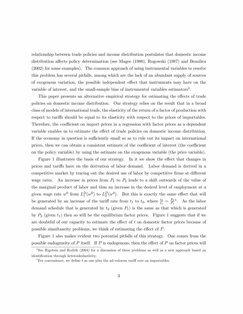
Figure 1 illustrates the basis of our strategy. In it we show the effect that changes in

prices and tariffs have on the derivation of labor demand. Labor demand is derived in a

competitive market by tracing out the desired use of labor by competitive firms at different

wage rates. An increase in prices from P1 to P2 leads to a shift outwards of the value of

the marginal product of labor and thus an increase in the desired level of employment at a

given wage rate w0 from LD1 (w0) to LD2 (w

0). But this is exactly the same effect that will

be generated by an increase of the tariff rate from t1 to t2, where t2t1= P2

P14. As the labor

demand schedule that is generated by t2 (given P1) is the same as that which is generated

by P2 (given t1) then so will be the equilibrium factor prices. Figure 1 suggests that if we

are doubtful of our capacity to estimate the effect of t on domestic factor prices because of

possible simultaneity problems, we think of estimating the effect of P .

Figure 1 also makes evident two potential pitfalls of this strategy. One comes from the

possible endogeneity of P itself. If P is endogenous, then the effect of P on factor prices will3See Rigobón and Rodrik (2004) for a discussion of these problems as well as a new approach based on

identification through heteroskedasticity.4For convenience, we define t as one plus the ad-valorem tariff rate on importables.

3

be no easier to estimate than that of t, leaving little value added to our approach. We will

adress this problem by restricting the estimation to small countries, for which the assumption

of exogenous terms of trade is quite appealing. A second pitfall comes form the possibility

that P may cause subsequent shifts in t. If t moves in tandem with P , then it will be

econometrically difficult to disentangle their effects. However, as long as we believe that

exogeneity of P is a tenable assumption, it will be easy to verify whether this correlation

exists in practice, and whether the necessary conditions for our estimation approach are

validated.

Additional complications can arise if factor supplies are income-elastic or if some goods

are non-traded. The reason is that tariffs and international prices do have non-symmetric

effects on aggregate income, so that any type of income effects wil introduce a wedge between

the price elasticity and the tariff elasticity of factor returns. However, as we show below, it

is possible to quantify this bias and to ascertain the magnitude of the difference between the

two coefficients, preserving the validity of our estimation strategy.

We illustrate our approach through empirical tests of competing theories of the relation-

ship between trade and factor prices using data on factor shares of capital and labor in 109

economies for the period between 1960 and 1999 from the United Nations’ System of National

Accounts. Using data on multilateral trade flows, we are able to distinguish between countries

that control a significant share of the market for their exports or imports and those that do

not. For the latter group, our identification assumption enables us to use the coefficient

on a country’s terms of trade to estimate the effect of trade restrictions on domestic income

distribution.

Our results do not support the predictions of neoclassical trade theory. We find that

the coefficient on international prices in poor economies is statistically undistinguishable

from that in rich economies, so that the data do not indicate the existence of a distinction

between the effect of trade that varies with a country’s capital abundance, as implied by

the Stolper-Samuelson theorem. These results hold both in the complete data set as well as

in Gollin’s (2002) income shares corrected for self-employment, which are available for 25

of the economies in our sample. On the other hand, our data offers suggestive evidence in

favor of the existence of an interaction between economic integration and the wage bargaining

4

process: we find that countries are more likely to see capital shares increase with openness

when their labor force is highly unionized, a result that is consistent with the predictions of

a wage-bargaining model of relative factor returns.

The rest of the paper proceeds as follows. Section 2 presents our key theoretical results,

establishing the conditions under which the elasticities of factor returns with respect to the

terms of trade are identical to those with respect to the terms of trade, and quantifying the

potential bias when those conditions do not hold. Section 3 develops our empirical strategy

and presents our empirical results. Section 5 concludes.

2 Trade and factor prices: theoretical links

The relationship between trade and factor prices in trade-theoretic models forms an extensive

body of literature that is aptly surveyed, among others, by Dixit and Norman (1980), Jones

and Neary(1984), Ethier (1984) and Feenstra (2004). We appeal to some well-known results

of this literature to establish the conditions under which our identification assumption - that

the price and tariff elasticities of factor returns are equal - holds. As we will show, these two

elasticities will be equal whenever all goods are traded and factor supplies do not depend on

income levels. When we allow for non-traded goods and income-responsive factor supplies,

the equality will break down; however, we will derive conditions which will help us to quantify

and control for the difference between these two coefficients.

Let there beM factors of production and I goods. Let w = {w1...wM}0 denote the vectorof factor returns for each of the M factors of production. Likewise, let the use of each of the

M factors by industry i be captured by the vector Bi = {B1i...BMi}0. Production is givenby the vector of production functions q = {F1(B1)...FI(BI)}0, and price levels in the vectorp = {p1...pI}0. Factor supplies are given by Bs = {Bs1, ...BsM}0 . Firms are price-takers

and profit-maximizers, and perfect competition implies free entry and zero profits. The

unit cost function for industry i will be ci(w) = minBi≥0w0Bi subject to Fi(Bi) = 1. Let

c = {c1(w)...cI(w)}0. p∗ = {p∗1...p∗I}0 is the vector of international prices and T = diag{t}is an I × I diagonal matrix with one plus the ad-valorem tariff rate for good i, ti on the

i-th term of the diagonal. Thus the I × 1 vector Tp∗ will give us the tariff-inclusive priceof imported goods. If good i is exported in equilibrium, then ti > 0 should be taken to

5

indicate an export subsidy. Equilibrium will be given by the w and q vectors that satisfy

the I zero-profit conditions and the M factor market equilibrium conditions:

p = c(w) (1)

A(w)q = Bs, (2)

where A is the M × I matrix with component aij(w) = ∂cj∂wi

in the i-th row and j-th

column. (1) and (2) provide a system of M + I equations in the M + I variables w and q.5

2.1 No income effects

We start out by considering the case in which all goods are tradable and factor supplies are

given. In this case Bs = {B1, ...BM}0, a vector of fixed factor supplies, and p = Tp.Let us first look at the case of ”even” technologies, where I = M so that there are as

many goods as factors. Equation (1) now defines a system of I equations in M = I variables.

The implicit function theorem implies that, if c1(w)...cI(w) are Ck−functions in RI anddet|A0| 6= 0 at a solution {p0,w0} then (1) defines w as a Ck−function of p and:

∂w

∂p=¡A0¢−1

.

Let εxy denote the elasticity of x with respect to y. Then the chain rule implies that

εwjy = εwjpiεpiy for y = {p∗i , ti}. As pi = tip∗i , then εpip∗i = εpiti = 1, allowing us to establish

our result6:

εwjp∗i = εwjti , (3)

that is, the elasticity of wages with respect to trade restrictions will be the same as its

elasticity with respect to international prices. In the case of two factors of production (call5Economies of scale can be accommodated by writing the unit cost function as c(w,q). The reasoning

presented for the I 6=M case would hold, although the sense of an equation such as (1) might be thrown into

question. Section 2.3 presents a special case in which (1) need not hold.6Note that we have simply assumed det |A0| 6= 0 instead of the more restrictive Nikaido (1972) conditions.

The reason is that for our result to hold we do not require uniqueness of w; even if there is more than one

wage vector consistent with a given price vector, equation (3) will be true for small changes in the price level

at a particular equilibrium.

6

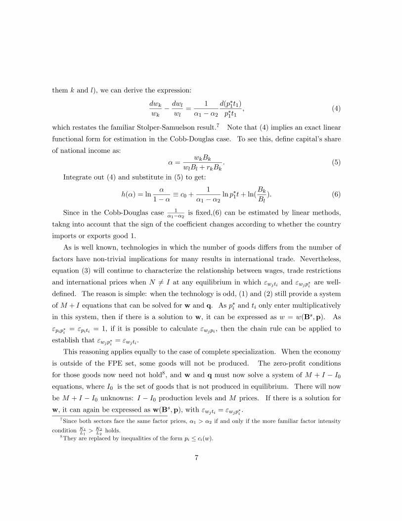
them k and l), we can derive the expression:

dwkwk− dwlwl

=1

α1 − α2

d(p∗1t1)p∗1t1

, (4)

which restates the familiar Stolper-Samuelson result.7 Note that (4) implies an exact linear

functional form for estimation in the Cobb-Douglas case. To see this, define capital’s share

of national income as:

α =wkBk

wlBl + rkBk. (5)

Integrate out (4) and substitute in (5) to get:

h(α) = lnα

1− α≡ c0 + 1

α1 − α2ln p∗1t+ ln(

BkBl). (6)

Since in the Cobb-Douglas case 1α1−α2 is fixed,(6) can be estimated by linear methods,

takng into account that the sign of the coefficient changes according to whether the country

imports or exports good 1.

As is well known, technologies in which the number of goods differs from the number of

factors have non-trivial implications for many results in international trade. Nevertheless,

equation (3) will continue to characterize the relationship between wages, trade restrictions

and international prices when N 6= I at any equilibrium in which εwjti and εwjp∗i are well-

defined. The reason is simple: when the technology is odd, (1) and (2) still provide a system

of M + I equations that can be solved for w and q. As p∗i and ti only enter multiplicatively

in this system, then if there is a solution to w, it can be expressed as w = w(Bs,p). As

εpip∗i = εpiti = 1, if it is possible to calculate εwjpi , then the chain rule can be applied to

establish that εwjp∗i = εwjti .

This reasoning applies equally to the case of complete specialization. When the economy

is outside of the FPE set, some goods will not be produced. The zero-profit conditions

for those goods now need not hold8, and w and q must now solve a system of M + I − I0equations, where I0 is the set of goods that is not produced in equilibrium. There will now

be M + I − I0 unknowns: I − I0 production levels and M prices. If there is a solution for

w, it can again be expressed as w(Bs,p), with εwjti = εwjp∗i .7Since both sectors face the same factor prices, α1 > α2 if and only if the more familiar factor intensity

condition K1L1> K2

L2holds.

8They are replaced by inequalities of the form pi ≤ ci(w).

7

It may well be the case, however, that it is not possible to find a solution to the system

defined by (1) and (2). This will generally be the case when I > M , as then (1) provides

a system of I equations in M variables, which have no solution except for very special price

vectors. Obviously, our result cannot be derived in such a case, not because εwjti and εwjp∗iare different, but because they do not exist. However, some authors have argued that in this

case of inexistence of equilibrium, international prices will adjust to levels consistent with

positive production of all goods (see Dixit and Norman, 1980). In such a case, I −M zero

profit conditions become redundant and the remainingM conditions can be solved as before.

Even though production levels will be indeterminate, factor prices will not, and the equality

between εwjti and εwjp∗i will be maintained.

We summarize our results in the following Proposition

Proposition 1 Let all goods be traded and factor supplies be given. Then if there is a

solution for w in the system of equations given by (1) and (2) and at that equilibrium εwjpi

exists, then εwjp∗i = εwjti.

2.2 Income effects

The equivalence between εwjti and εwjp∗i can be broken if income levels are allowed to af-

fect domestic wages. The reason is that international prices and tariff rates affect income

differently: an increase in the terms of trade can shift a country’s consumption possibili-

ties set outwards, but an increase in tariffs cannot. In other words, the one equation in

which international prices and tariffs do not enter multiplicatively is that pertaining to the

determination of aggregate GDP:

Y = w0Bı+ ı0ΠM

where B is an N × I matrix whose columns are the factor use vectors Bi, ı is an I ×1 vector of ones, Π is a diagonal matrix with pi(ti − 1) in each of the i diagonal terms,and M = D(Y ,p)− q a vector of import levels, where D(Y,p) denotes aggregate economydemand for good i.

Let us first think about the income effects that operate through factor supplies. Let

Bs= Bs(w,p,Y ). Note first that whenever (1) can be solved for w then Bs has no effect

8

whatsoever on factor prices, and whether it depends on Y or not is irrelevant. Therefore,

if I = M and the conditions necessary for the implicit function theorem to be applied hold,

then εwjti = εwjp∗i .

This will also be true when I > M if it is the case that international prices are such

that there is positive production of all goods in the home country, as then the number of

linearly independent zero-profit conditions reduces to M . It cannot, however, be applied

when I < M . In such a case, equilibrium w, q and Y must solve:

Tp∗ = c(w) (7)

A(w)q = Bs(w,Tp∗,Y) (8)

Y = w0Bı+ ı0ΠM. (9)

Note that if there exists a solution to this system, there also must be a solution to the

subsystem formed by the first I +M equations for w and q as a function of Tp∗ and Y .

Therefore, it must be the case that

εwjp∗i − εwjti = εwjY¡εY p∗i − εY ti

¢. (10)

Letting FI(Tp∗, Y ) = w(Tp∗, Y )0Bı denote domestic factor income gives us an implicit

solution for the equilibrium Y as a function of p∗i and ti (provided of course that the conditions

of the implicit function theorem are satisfied):

Y = FI(Tp∗, Y ) +Xi

p∗i (ti − 1)Mi(Tp∗, Y ). (11)

Taking derivatives with respect to p∗i and ti, subtracting, reorganizing and substituting in

(10) gives us:

εwjp∗i = εwjti − εwjY1

1− FIY −Pj P

∗j (tj − 1)M j

Y

mi. (12)

where mi = P∗i Mi/Y is the ratio of industry i imports to GDP at world prices. (12) will be

extremely important in our estimation strategy, as it allows us to quantify the potential bias

that can arise from using εwkp∗i as an estimator of εwkti − εwlti .

We turn now to the case of income effects that operate through the demand for non-

tradables. When some goods are not traded internationally, their prices become endogenous,

9

and must be determined by clearing of the domestic market. (7) now becomes:

pi = ci(w) for i ∈ NT (13)

p∗i ti = ci(w) for i ∈ T,

with (8) and (9) as above, but with a new set of NT additional market clearing conditions:

Di(p, Y ) = Qi for i ∈ NT. (14)

(8),(9), (13) and (14) now form a system ofM+I+NT+1 equations that can be solved for the

M factor returns, I production levels, NT domestic prices and income Y . As before, the first

M+I+NT equations can be solved for w = w(Tp∗, Y ),q = q(Tp∗, Y ) and p = p(Tp∗, Y ).

The above reasoning can now be applied to derive (12). The results are summarized in

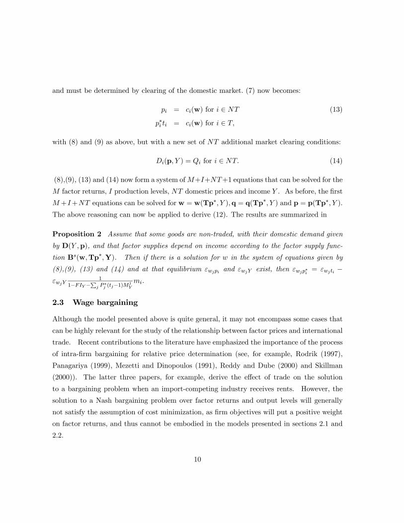
Proposition 2 Assume that some goods are non-traded, with their domestic demand given

by D(Y ,p), and that factor supplies depend on income according to the factor supply func-

tion Bs(w,Tp∗,Y). Then if there is a solution for w in the system of equations given by

(8),(9), (13) and (14) and at that equilibrium εwjpi and εwjY exist, then εwjp∗i = εwjti −εwjY

1

1−FIY − j P∗j (tj−1)Mj

Y

mi.

2.3 Wage bargaining

Although the model presented above is quite general, it may not encompass some cases that

can be highly relevant for the study of the relationship between factor prices and international

trade. Recent contributions to the literature have emphasized the importance of the process

of intra-firm bargaining for relative price determination (see, for example, Rodrik (1997),

Panagariya (1999), Mezetti and Dinopoulos (1991), Reddy and Dube (2000) and Skillman

(2000)). The latter three papers, for example, derive the effect of trade on the solution

to a bargaining problem when an import-competing industry receives rents. However, the

solution to a Nash bargaining problem over factor returns and output levels will generally

not satisfy the assumption of cost minimization, as firm objectives will put a positive weight

on factor returns, and thus cannot be embodied in the models presented in sections 2.1 and

2.2.

10

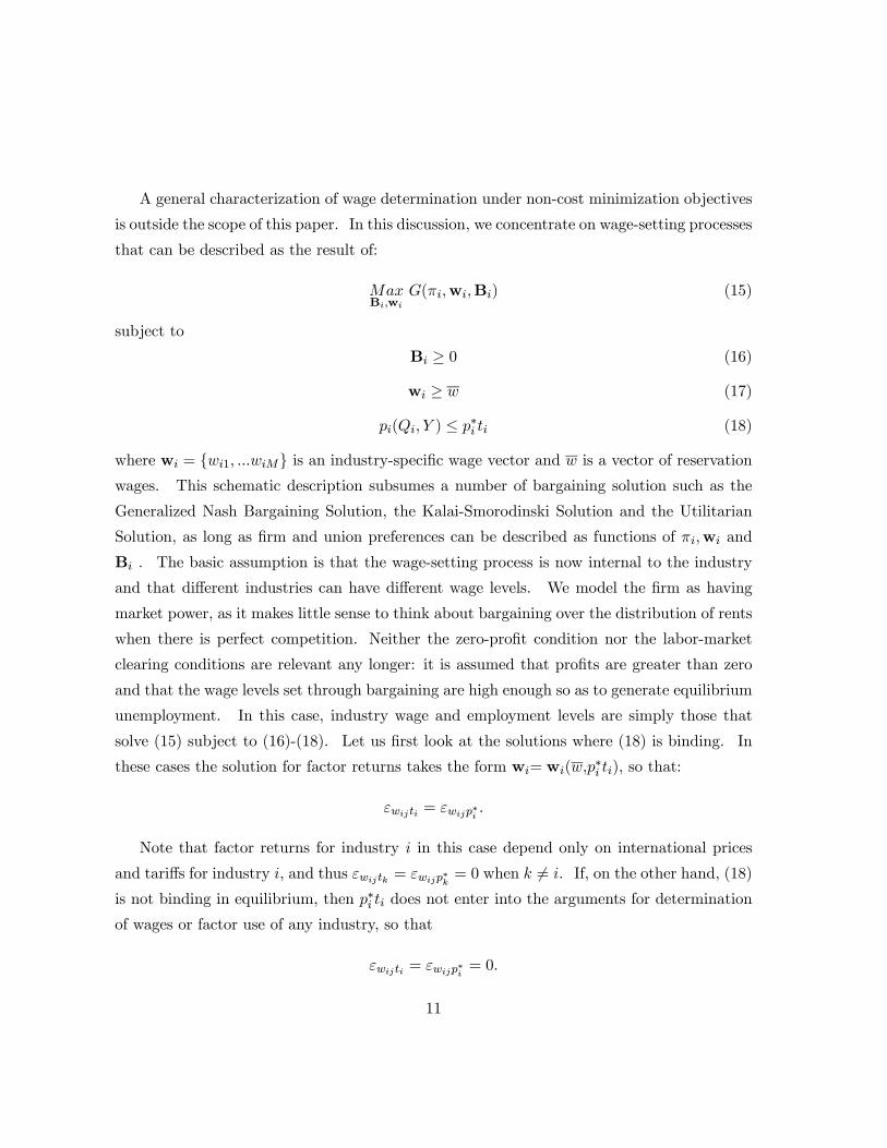
A general characterization of wage determination under non-cost minimization objectives

is outside the scope of this paper. In this discussion, we concentrate on wage-setting processes

that can be described as the result of:

MaxBi,wi

G(πi,wi,Bi) (15)

subject to

Bi ≥ 0 (16)

wi ≥ w (17)

pi(Qi, Y ) ≤ p∗i ti (18)

where wi = {wi1, ...wiM} is an industry-specific wage vector and w is a vector of reservationwages. This schematic description subsumes a number of bargaining solution such as the

Generalized Nash Bargaining Solution, the Kalai-Smorodinski Solution and the Utilitarian

Solution, as long as firm and union preferences can be described as functions of πi,wi and

Bi . The basic assumption is that the wage-setting process is now internal to the industry

and that different industries can have different wage levels. We model the firm as having

market power, as it makes little sense to think about bargaining over the distribution of rents

when there is perfect competition. Neither the zero-profit condition nor the labor-market

clearing conditions are relevant any longer: it is assumed that profits are greater than zero

and that the wage levels set through bargaining are high enough so as to generate equilibrium

unemployment. In this case, industry wage and employment levels are simply those that

solve (15) subject to (16)-(18). Let us first look at the solutions where (18) is binding. In

these cases the solution for factor returns takes the form wi= wi(w,p∗i ti), so that:

εwijti = εwijp∗i .

Note that factor returns for industry i in this case depend only on international prices

and tariffs for industry i, and thus εwijtk = εwijp∗k = 0 when k 6= i. If, on the other hand, (18)is not binding in equilibrium, then p∗i ti does not enter into the arguments for determination

of wages or factor use of any industry, so that

εwijti = εwijp∗i = 0.

11

However, there may still be income effects arising from the impact that tariffs on other

industries can have on income levels Y and thus on demand for industry i’s good, so that:

εwijp∗k = εwijtk − εwijY1

1− FIY −Pl P

∗l (tl − 1)M l

Y

mk for k 6= i. (19)

The results related to the general wage bargaining problem are summarized in

Proposition 3 Let wage-setting in industry i be defined by the solution to (15)-(18). At any

solution to this problem:

(i) if εwijpk exists and(18) is binding then εwijtk = εwijp∗k for all i, j. Furthermore,εwijtk =

εwijp∗k = 0 when k 6= i.(ii) If εwijpk and εwijY exist and (18) is not binding, then εwijtk = εwijp∗k = 0 when k = i.

Furthermore, εwijp∗k = εwijtk − εwijY1

1−FIY − l P∗l (tl−1)M l

Y

mk when k 6= i.

2.3.1 A simple example

The above model of wage bargaining is too general to allow us to draw testable empirical

implications. In order to get an idea of the basic mechanisms at work in the wage bargaining

framework, we specialize to a simple two factor model (j = {l, k}) in which the productiontechnology is Leontieff and income effects on factor supply are absent. Firm profits are:

πi = (pi(qi)−wli − wr)Bli,

where wr is the market interest rate. We assume that p∗i ti − wr > wl, so that there

effectively exist rents over which to bargain. Bargaining takes place between the firm and a

domestic union which seeks to maximize:

Ui = (wli − wl)δBli.

The equilibrium will be given by the solution of the Generalized Nash Bargaining problem:

Maxli,wi

a ln [(pi(Bli)−wli − wr)Bli] + (1− a) lnh(wli −wl)δBli

isubject to

p(Bli) ≤ p∗i ti, wli ≥ wl.

12

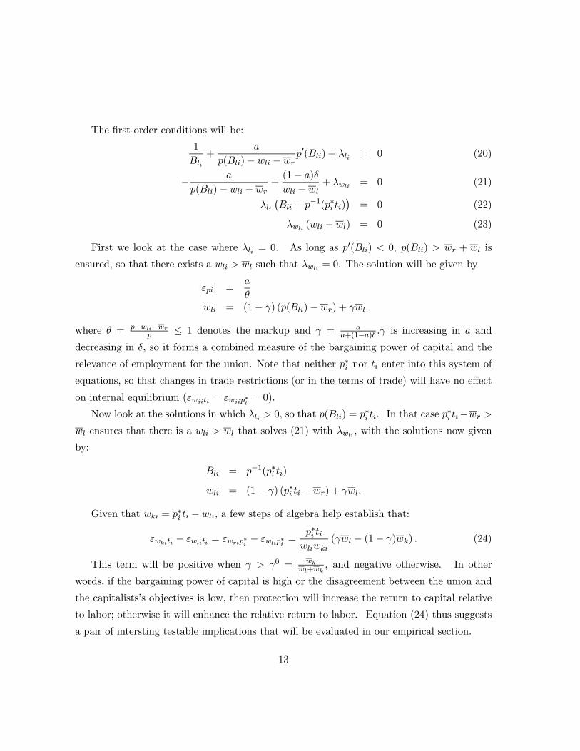
The first-order conditions will be:

1

Bli+

a

p(Bli)− wli − wr p0(Bli) + λli = 0 (20)

− a

p(Bli)− wli −wr +(1− a)δwli − wl + λwli = 0 (21)

λli¡Bli − p−1(p∗i ti)

¢= 0 (22)

λwli (wli − wl) = 0 (23)

First we look at the case where λli = 0. As long as p0(Bli) < 0, p(Bli) > wr + wl is

ensured, so that there exists a wli > wl such that λwli = 0. The solution will be given by

|εpi| =a

θwli = (1− γ) (p(Bli)− wr) + γwl.

where θ = p−wli−wrp ≤ 1 denotes the markup and γ = a

a+(1−a)δ .γ is increasing in a and

decreasing in δ, so it forms a combined measure of the bargaining power of capital and the

relevance of employment for the union. Note that neither p∗i nor ti enter into this system of

equations, so that changes in trade restrictions (or in the terms of trade) will have no effect

on internal equilibrium (εwjiti = εwjip∗i = 0).

Now look at the solutions in which λli > 0, so that p(Bli) = p∗i ti. In that case p

∗i ti−wr >

wl ensures that there is a wli > wl that solves (21) with λwli , with the solutions now given

by:

Bli = p−1(p∗i ti)

wli = (1− γ) (p∗i ti − wr) + γwl.

Given that wki = p∗i ti − wli, a few steps of algebra help establish that:

εwkiti − εwliti = εwrip∗i − εwlip∗i =p∗i tiwliwki

(γwl − (1− γ)wk) . (24)

This term will be positive when γ > γ0 = wkwl+wk

, and negative otherwise. In other

words, if the bargaining power of capital is high or the disagreement between the union and

the capitalists’s objectives is low, then protection will increase the return to capital relative

to labor; otherwise it will enhance the relative return to labor. Equation (24) thus suggests

a pair of intersting testable implications that will be evaluated in our empirical section.

13

3 Estimation

In this section we will provide an illustration of our empirical method using data on the

shares of labor and capital income in aggregate factor income taken from United Nations

(2000), which compiles national accounts statistics elaborated according to its System of

National Accounts for 117 countries. Data on import duties, export taxes and trade/GDP

ratios come from World Bank (2002). The terms of trade variable is constructed as the

quotient of the GDP deflators for export and import prices from the national accounts data.

Depending on the specification, our baseline regressions cover between 88 and 103 countries.

The data are divided into five-year averages for the 1960-1999 period, in order to diminish

the possible contamination from business cycle effects. We use import and export volume

data for every country at the 2-digit level from the COMTRADE database (United Nations,

2004) to construct an index of international market power by country. This index is simply

the weighted average of the country’s export (import) share in world exports (imports) by

product, where the weights are the product’s share in the country’s exports (imports). We

define a country as large of it has a value greater than 0.1 in either the export-based or the

import-based index. The resulting list of large countries includes 7 economies: USA, Japan,

Germany, Saudi Arabia, Colombia, UK and Canada.9

Section 2 has described the links between international prices, trade restrictions and

domestic factor prices that arise in the general case of many commodities and goods. The

data that we will use in our paper refer to the shares in national income accounts of two

factors of production, which, following convention, we call capital (k) and labor (l). The

first necessary step in order to set up our estimation strategy is to transform our results into

testable implications regarding the shares of these two factors in aggregate income.9An eight economy (South Africa) also appears as large in this index because it accounts for 60% of world

exports and 29% of world imports of commodity class S2-93 ”Special transactions, commodity not classified

according to class. ” This is an artifact of the large level of unclassified trade occurring in the South African

Customs Union and is not indicative of any significant level of market power. We tried other specifications

(with and without South Africa and using other thresholds for market power), with none of them yielding

significant differences from the specification reported.

14

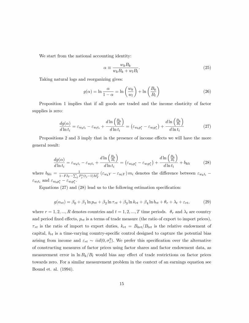
We start from the national accounting identity:

α ≡ wkBkwkBk + wlBl

. (25)

Taking natural logs and reorganizing gives:

g(α) = lnα

1− α= ln

µwkwl

¶+ ln

µBkBl

¶(26)

Proposition 1 implies that if all goods are traded and the income elasticity of factor

supplies is zero:

dg(α)

d ln ti= εwkti − εwlti +

d ln³BkBl

´d ln ti

=¡εwkp∗i − εwlp∗i

¢+d ln

³BkBl

´d ln ti

(27)

Propositions 2 and 3 imply that in the presence of income effects we will have the more

general result:

dg(α)

d ln ti= εwkti − εwlti +

d ln³BkBl

´d ln ti

=¡εwkp∗i − εwlp∗i

¢+d ln

³BkBl

´d ln ti

+ bkli (28)

where bkli = 1

1−FIY − j P∗j (tj−1)Mj

Y

(εwkY − εwlY )mi denotes the difference between εwkti −εwlti and εwkp∗i − εwlp∗i .

Equations (27) and (28) lead us to the following estimation specification:

g(αrt) = β0 + β1 ln prt + β2 ln τ rt + β3 ln krt + β4 ln brt + θr + λt + εrt, (29)

where r = 1, 2, ..., R denotes countries and t = 1, 2, ..., T time periods. θr and λt are country

and period fixed effects, prt is a terms of trade measure (the ratio of export to import prices),

τ rt is the ratio of import to export duties, krt = Bkrt/Blrt is the relative endowment of

capital, brt is a time-varying country-specific control designed to capture the potential bias

arising from income and εrt ∼ iid(0,σ2ε). We prefer this specification over the alternative

of constructing measures of factor prices using factor shares and factor endowment data, as

measurement error in lnBk/Bl would bias any effect of trade restrictions on factor prices

towards zero. For a similar measurement problem in the context of an earnings equation see

Bound et. al. (1994).

15

Several points are worth noting with respect to this specification. The first one is that our

preferred functional form for estimation uses the logarithmic transformation g(α) = ln³

α1−α

´as the dependent variable. This functional form is derived above from the accounting identity

(25) and has the implication that the coefficients of ln pit and ln τ it will be equal to the

elasticities that Proposition 1-3 refer to, regardless of the functional forms taken by the

unit cost and factor supply functions. A more common approach in the literature is to

derive the equation to be estimated form the translog specification for the GDP function

(see Kohli, 1990, 1991). This specification can cause severe consistency problems if the

translog functional form is incorrect. The reason is that by definition factor shares are

bounded between 0 and 1, and when estimating an equation like (29), standard assumptions

about the disturbance εrt (such as normality) require an unbounded support, something that

is in contradiction with the dependent variable being restricted to the unit interval. The

logit transform of the dependent variable (as suggested by Davidson and MacKinnon, 1993)

allows it to take on values anywhere on the real line. Although this fact is well understood

in the context of linear probability models with unbounded explanatory variables, it is often

disregarded in other applied settings (for an exception, see Emmons and Schmid, 2000). The

choice of specification, however, is not crucial to our results, and we provide below estimates

for the more common tranlog GDP function functional form.

A second point that we wish to call attention to is that our terms of trade indicator is

by definition country-specific, as it is built using prices of exports and imports taken from

national income accounts. Therefore these indexes are not comparable across countries,

making the cross-sectional variation among them meaningless. This is the reason for which

we do not present random effect estimates in our results10.

In the third place, the results of Propositions 1-3 form the backbone of our identifica-

tion strategy. In particular, we assume that εwkp∗i − εwlp∗i provides a reasonable estimate of

εwkti − εwlti , as long as the potential bias arising from income effects is appropriately con-

trolled for. The theoretical results support the argument that this is a reasonable assumption

for a broad subset of theories of international trade that subsumes the theories that we want

to evaluate, such as Stolper-Samuelson and wage bargaining. In this sense, our approach of10Hausmann specification tests without the price variable also favor the fixed effects specification.

16

identification through theory is similar to that of authors like Levitt and Porter (2001), who

impose reasonable restrictions on observed behavior of individual agents in order to derive

identification assumptions, and contrasts with the use of instrumental variables with exoge-

nous instruments common in cross-country empirical studies and perhaps best exemplified

by contributions such as those of Frankel and Romer (2000) and Acemoglu, Johnson and

Robinson (2001).

Notice that we do not impose the restriction that β1 = −β2 in our model, which is whatour identification assumption may be taken to imply. The reason is that if τ rt is endogenous,

β2 will be difficult to estimate empirically and imposing such a restriction will bias our

estimate of β1. Instead, we know that as long as we restrict ourselves to the case of small

countries, shocks to prt will be exogenous to the process determining income shares within

an economy, so E[prtεrt] = 0, guaranteeing identification of β1 even if E[τ rtεrt] 6= 0, providedappropriate controls for ln(Bk/Bl) and brt are included11.

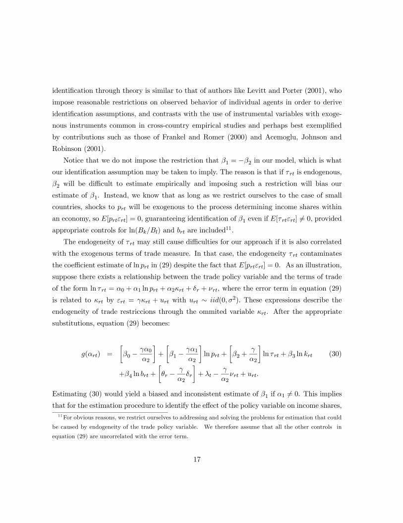
The endogeneity of τ rt may still cause difficulties for our approach if it is also correlated

with the exogenous terms of trade measure. In that case, the endogeneity τ rt contaminates

the coefficient estimate of ln prt in (29) despite the fact that E[prtεrt] = 0. As an illustration,

suppose there exists a relationship between the trade policy variable and the terms of trade

of the form ln τ rt = α0 + α1 ln prt + α2κrt + δr + νrt, where the error term in equation (29)

is related to κrt by εrt = γκrt + urt with urt ∼ iid(0,σ2). These expressions describe the

endogeneity of trade restriccions through the ommited variable κrt. After the appropriate

substitutions, equation (29) becomes:

g(αrt) =

∙β0 −

γα0α2

¸+

∙β1 −

γα1α2

¸ln prt +

∙β2 +

γ

α2

¸ln τ rt + β3 ln krt (30)

+β4 ln brt +

∙θr − γ

α2δr

¸+ λt − γ

α2νrt + urt.

Estimating (30) would yield a biased and inconsistent estimate of β1 if α1 6= 0. This impliesthat for the estimation procedure to identify the effect of the policy variable on income shares,11For obvious reasons, we restrict ourselves to addressing and solving the problems for estimation that could

be caused by endogeneity of the trade policy variable. We therefore assume that all the other controls in

equation (29) are uncorrelated with the error term.

17

it is important that the exogenous variable be uncorrelated with the endogenous variable of

interest.

Fortunately, whether this is the fact or not can be verified by running a regression of

ln τ rt on ln prt, κrt and a set of country fixed effects. Since we can safely assume exogeneity

of ln prt, such a regression allows us to accurately estimate α1 as long as the relevant κrt are

controlled for. This regression would be analogous to the first-stage regressions common

in implementations of instrumental variables techniques. But unlike conventional first-stage

regressions, the necessary condition for the validity of our approach would be established

by failing to find a significant coefficient for ln prt. It is only in this way that we can be

certain that the coefficient estimate on ln prt in (30) will not be contaminated by the potential

endogeneity of (30) (i.e., that α1 = 0)

Such a set of regressions is reported in Table 1. We report equations for the whole sample

and for sample splits distinguishing poor and rich countries, as well as with and without a

full set of controls. Both the criteria for splitting the sample and the list of controls parallel

those used in the estimates of (30) reported below. The results confirm a lack of association

between the terms of trade indicator and the trade policy variable: the coefficient on ln prt

is never significant, and the lowest p-value it attains is 0.303.

It is worth noting that one advantage of our approach over the IV approach is that it

allows us to get away from the small-sample bias of instrumental variables estimators. As

is well-know, instrumental variables estimators are consistent, but they are also biased (see

Davidson and Mackinnon, 1993). Cross country datasets are naturally of limited size, so

inference based on IV estimates is weak at best. Our approach, in contrast, provides an

estimate that is both consistent and unbiased under the aforementioned models. This makes

inference about the effects of a policy variable such as trade policy much more reliable.

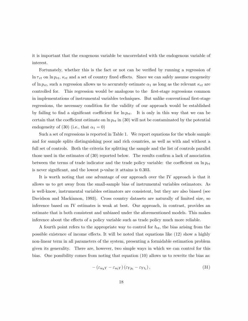
A fourth point refers to the appropriate way to control for brt, the bias arising from the

possible existence of income effects. It will be noted that equations like (12) show a highly

non-linear term in all parameters of the system, presenting a formidable estimation problem

given its generality. There are, however, two simple ways in which we can control for this

bias. One possibility comes from noting that equation (10) allows us to rewrite the bias as:

− (εwkY − εwlY ) (εY pi − εY ti) , (31)

18

which shows that the bias is caused by the indirect effect that tariffs and external prices have

on relative factor returns through Y . These effects are due to fact that the only place in the

system of equations determining w where p∗i and ti do not enter multiplicatively is in the

equation for Y , (9). (31) therefore suggests controlling for Y when we estimate a regression

of g(α) on p∗i . An alternative comes from taking a first-order Taylor approximation of (12)

around mi = 0, which reduces us:

bkli ∼= 1

1− FI0Y¡ε0wkY − ε0wlY

¢mi, (32)

an expression which is proportional to mi. (32) implies that an appropriate way to control

for the bias is to introduce an interaction term between ln pit and mi in the regresion. Given

that when mi < 0, ti corresponds to an export subsidy, the appropriate empirical counterpart

of mi is the share of exports plus imports in GDP.

One last point that we wish to emphasize is that the nature of our data naturally limits

its ability to deal with the effects of trade policy on the distribution of income when there are

more than two factors of production. The results that follow should be read as a comparative

evaluation of the explanatory power of two-factor models of international trade. Despite this

limitation, there is nothing in our empirical strategy that impedes its application to multi-

factor contexts, and we view our exercise as illustrative of the possibilities inherent in our

approach rather than as a definitive evaluation of existing theories.

3.1 Results

Table 2 displays the results of our first attempt to test for the existence of Stolper-Samuelson

effects in the data. Recall that the coefficient of interest is the one on the terms of trade

variable, which should be positive for capital abundant economies and negative for labor-

abundant economies. In this table, we use per capita GDP as our indicator of capital-

abundance; we explore other measures below. According to (31), controlling for per capita

GDP also allows us to take care of income effects. We estimate the coefficient through two

specifications: in the first one (columns 1 and 2) we split the sample into labor-abundant and

capital-abundant countries,12 while in the second one (column 3) we introduce an interaction12A country is labor (capital) abundant if its per capita GDP is below (above) world per capita GDP.

19

term between the capital abundance indicator and the terms of trade variable. Columns 4-6

repeat these regressions but with an additional direct control for the bias term bkl, which is an

interaction term between the trade share and the terms of trade variable, as suggested by (28).

These first results should be disappointing for Stolper-Samuelson advocates. The coefficient

on the terms of trade variable is insignificant and has the wrong sign for labor-abundant

countries regardless of whether the direct control for bkl is introduced or not. For capital-

abundant countries, there is a positive and significant coefficient, as expected by theory, in

column 2, but it disappears and becomes negative though not significant as soon as the bias

control term is introduced, with that term being strongly significant. As to the interaction

term between terms of trade and capital abundance, it is insignificant and the sign becomes

negative when the bias control is introduced.

Table 3 confirms the results of Table 2 using the conventional translog-GDP function

approach, which has the capital share (instead of the logit transform) as the dependent

variable. The results are very similar in terms of sign and statistical significance of the

coefficients on the terms of trade, with the only substantial difference being that the sign of the

terms of trade variable in the regression for capital-abundant countries with the bias control

now becomes significantly negative, in contradiction to the expected positive coefficient.

In a recent paper, Gollin (2002) has argued that standard national accounting significantly

misrepresents income shares by classifying income from self-employment as capital income.

Therefore some countries may falsely appear to have high capital shares due to the existence

of a large informal sector. Gollin produces a set of adjustments to income shares for a

reduced subset of economies for which data on the income from unincorporated enterprises

is available. In order to make sure that our results are not due to the bias arising from

this misclassification of self-employment, we repeat our tests of Tables 2 and 3 on the Gollin

data.13 None of the six coefficients reported in this table are significantly different from

zero. Some comfort may be taken from the fact that all but one of the coefficients have the

sign indicated by theory; on the other hand the coefficients are very far from conventional13We use Gollin’s first adjustment, which imputes all income from unincorporated enterprises as labor

income. Results are similar if one uses his second adjustment (impute same labor share as the rest of the

economy); his third adjustment (which imputes a wage for proprietors and self-employed individuals), however,

yields insufficient observations for our estimation.

20

significance levels (the average p-value for the six coefficients of interest is 0.67).

One possible explanation for these results is that some countries may be completely

specialized in a subset of goods, invalidating the assumption of factor price equalization that

is the backbone of the Stolper-Samuelson model. Fortunately, factor price equalization is not

a necessary condition for our identification assumptions to be valid, allowing us to apply to

modified versions of the Stolper-Samuelson theorem that apply in a setting of multiple cones

of diversification. As shown by Davis (1996) and Xu (2000), among others, what is relevant

in a world of multiple cones of diversification is a country’s level of capital abundance relative

to its cone of diversification. Table 5 makes a first attempt to address this issue: in it we split

the sample further into two groups, corresponding respectively to above and below world

per-capita GDP. This would correspond with the existence of two symmetrically distributed

cones of diversification. Within each cone, we run the same six regressions as in Tables 2-4.

For the capital-abundant cone, four of the six coefficients have the wrong sign, one of them

being significant, while for the labor-abundant cone, none of the coefficients are significant

and two have the wrong sign.

A potential problem with this test is that it assumes the existence of two cones of diver-

sification, while theory offers no guide as to the number of cones of diversification nor to the

dividing points between them. One way to address this issue is by trying to find whether

there is evidence of a cone of diversification of any size at each extreme of the distribution

of capital abundance. Figures 2 and 3 show our attempt to do so. Figure 2 graphs the

coefficient and t-statistics on the interaction between the log of the terms of trade and the

log of per capita GDP taken from a regression identical to that reported in columns 6 and

12 of Table 5, but run for all possible definitions of the cone of diversification corresponding

to the highest range of capital-abundance. This means running 168 regressions, ranging

from the most restrictive definition of the capital-abundant cone (the one with the minimum

number of observations for which the regression can be run) to the most inclusive one (the

whole sample). Figure 3 does the same thing, but ranging from the most to least restrictive

definition for the labor-abundant cone. Recall that this interaction term should be positive

if the Stolper-Samuelson theorem holds. Figure 2 shows a striking fact: the coefficient on

the interaction is never significant and positive for any possible definition of the highest

21

capital-abundant cone of diversification. In the range in which the interaction is significant

(a range corresponding to 16-18 economies) the coefficient is actually negative, indicating

that the effect of trade on returns to capital decreases as capital intensity increases within

the cone. Figure 3 shows a similar fact for the lowest range of capital-abundance: with

the not very relevant exception of the first regression (which has one degree of freedom), no

other regression in this figure displays a significant coefficient, be it of the correct or incorrect

sign. Additional tests (not reported) replicate these results when we split each cone between

its capital-abundant and labor-abundant countries: for no definition of the most and least

capital-abundant cones of diversification is there a regression in which both coefficients are

significant and of the right sign.

In Table 6 we address some logical questions that might arise about our specification.

In the first place, we have used per capita GDP above as a control for capital abundance.

This is an admittedly rough measure of capital abundance. The first three columns of

Table 6 repeat our regressions using the Summers-Heston (1992) estimates of the capital

stock with the bias control term. Note that as these are unavailable in the latest version of

the Penn World Tables and are only compiled for a reduced number of countries, we lose a

significant number of observations when using this indicator: the number of countries in the

labor-abundant group fall from 42 to 20 and those in the capital-abundant group from 46 to

21. None of the three coefficients are significant and two have the wrong sign. The rest

of the columns experiment with additional specifications: columns 4-6 use Barro and Lee’s

(2004) measure of terms of trade instead of our national accounts based data; columns 7-9

use the share of imports and exports in GDP as our policy indicator, while columns 10-12

return to our baseline specification but add a set of alternative controls: for the level of

human capital (measured by the average years of secondary and higher schooling, the level of

political liberties and the right to bargain collectively. None of these additional specifications

particularly seem to favor Stolper-Samuelson: only two out of the nine specifications in

columns 4-12 have the right sign, and none of them are significant.

Given the disappointing performance of the Stolper-Samuelson hypothesis on our data, we

turn in Table 7 to identifying whether there is evidence of an effect of trade on domestic factor

prices that operates through the wage bargaining channel. As we showed in Section 2.3, the

22

effect of trade restrictions on factor shares should vary according to the relative bargaining

power of capital and labor. Therefore, we should expect to see trade increasing capital

shares in countries where labor organization is strong, whereas the opposite would happen

where it is weak. We use unionization rates from Rama and Artecona (2000) as our measure

of the degree of labor organization. Thus we introduce into the specification an interaction

between unionization levels and the log of the terms of trade variable. Since we are interested

in testing the wage bargaining model on its own (as opposed to a combination of it and the

Stolper-Samuelson model), the specification in Table 7 assumes that the coefficient on terms

of trade is the same for poor and rich countries14. We present six possible specifications

in this regression, corresponding to the three dependent variables in Tables 2-4, with and

without alternative controls. All of the estimates are positive, with three of them significant

at 5%. Even the non-significant coefficients are reasonably close to statistical significance

(p-values of .11, .29 and .14). The estimated effects are economically very significant: the

coefficient on the interaction term in equation 2, for example, implies that a country with a

unionization rate of 25.7% (the average of the sample) that raised tariffs from their free trade

level to an average level of 50% would see an increase of 5.9 percent of GDP in labor’s share

relative to a country with no unions.

These results suggest that there may be something to the wage bargaining story. Cer-

tainly, if viewed as a horse race between Stolper-Samuelson and wage bargaining theories,

wage bargaining has managed to leave Stolper-Samuelson behind, though partly thanks to

Stolper-Samuelson not running very fast (or, actually, that it seemed to be running in the

wrong direction). A fuller analysis of the empirical implications of the wage bargaining hy-

pothesis is beyond the scope of our paper. It is possible of course that unionization be

proxying for other variables that affect the trade-income distribution link. There may also

be problems of selection bias in the reporting of unionization data15. However, the fact

that a simple wage-bargaining theory does much better than neoclassical trade theory in this

initial horse race suggests that much of the effort directed at understanding the causes of14Tests allowing for different coefficients accoding to levels of income and capital intensity generate similar

results. Details are available upon request.15A simple selection model using real per capita GDP as the selection variable for non-missing values yields

similar results.

23

factor price movements may have been misplaced.

4 Concluding Remarks

This paper has proposed a simple strategy for identifying the effect of trade restrictions on

relative factor prices. In contrast to the common approach in the cross-national empirical lit-

erature, which addresses problems of identification by instrumenting on sources of exogenous

variation in policy variables, we derive our identification assumptions directly from theory.

As we have shown, a broad class of trade theories implies that the elasticity of factor returns

with respect to a tariff on good i should be identical to that with respect to an increase in

the price of good i. Even when these elasticities are not the same, theory suggests a way in

which we can quantify and control for the bias that could arise when we estimate the former

using the latter. The plausibility of the assumption of exogeneity of terms of trade changes

when the sample is restricted to small economies and the empirically verifiable fact that trade

policy and terms of trade are not correlated give us an opportunity to estimate the effect of a

policy variable using information on an exogenous variable, while at the same time avoiding

the small-sample bias of instrumental variables.

We have implemented our strategy on a cross-national panel of data on factor shares and

trade policy for more than one hundred economies. Our results are not supportive of the

Stolper-Samuelson theorem. As we have shown, Stolper-Samuelson effects are very hard to

find in the data, regardless of whether we look for them at the world level or at the level of

specific cones of diversification. In contrast, we do find evidence in the data that confirms the

predictions of wage-bargaining models whereby economic integration weakens the bargaining

power of unions.

Our results are naturally limited by the nature of our data, which reports income distrib-

ution for only two factors of production. One explanation for the disappointing results could

be that they are due to the incapacity of two-factor models for understanding the reaction of

factor prices to international trade. Indeed, our results can be seen as confirming the exten-

sive empirical literature that has systematically failed to confirm the empirical predictions

of the Heckscher-Ohlin-Vanek model. The methodology presented in this paper, however,

24

is applicable to multi-factor, multi-good contexts, suggesting a natural direction for future

research.

References

[1] Acemoglu,Daron, Simon Johnson and James A. Robinson (2001). ”The Colonial Origins

of Comparative Development: An Empirical Investigation,” American Economic Review,

American Economic Association, vol. 91(5), pages 1369-1401, December.

[2] Angrist Joshua. and Alan Krueger (2001) “Instrumental Variables and the Search for

Identification: From Supply and Demand to Natural Experiments.” Journal of Economic

Perspectives Vol. 15 No. 4.

[3] Bound, John, Charles Brown, Greg Duncan and Willard Rodgers (1994).“Evidence on

the Validity of Cross-sectional and Longitudinal Labor Market Data” Journal of Labor

Economics, vol. 12, no. 3, 345-368.

[4] Beaulieu, Eugene (2002) ”Factor or Industry Cleavages in Trade Policy? An Empirical

Analysis of the Stolper-Samuelson Theorem, ” Economics and Politics, 14(2): 99-131.

[5] Davidson, R., and J. MacKinnon. (1993). ”Estimation and Inference in Econometrics”.

Oxford University Press.

[6] Davis, Donald (1996) ”Trade Liberalization and Income Distribution. ” NBER Working

Paper 5693. Cambridge: National Bureau of Economic Research.

[7] Department of State (2003) “Commerce Secretary Says Free Trade Opens Doors

to Opportunity.” Press Release No. EPF418, Nov. 20, 2003. (http://usinfo.org/wf-

archive/2003/031120/epf418.htm).

[8] Dixit, Avinash and Victor Norman (1980) Theory of International Trade: A dual, general

equilibrium approach. Cambridge: Cambridge University Press.

[9] Emmons, William and Frank Schmid. “Banks vs. Credit Unions: Dynamic Competi-

tion in Local Markets.” Federal Reserve Bank of St. Louis, Working Paper 2000-006A,

February 2000.

25

[10] Ethier, Wilfred E. ”Higher Dimensional Issues in Trade Theory, ” in Jones, Ronald W.

Jones and Peter B. Keenen, eds (1984) Handbook of International Economics, Vol. I.

Amsterdam: North-Holland.

[11] Feenstra, Robert C. (2004) Advanced International Trade: Theory and Evidence. Prince-

ton: Princeton University Press.

[12] Frankel, Jeffrey and David Romer (1999) ”Does Trade Cause Growth? ” American

Economic Review 89(3): 379-399.

[13] Global Exchange (2003) “Top Ten Reasons to Oppose the Free Trade Area of the Amer-

icas”. Reproduced. San Francisco, CA: Global Exchange.

[14] Gollin, Douglas (2002) ”Getting Income Shares Right. ” Journal of Political Economy.

[15] Hanson, Gordon H. and Chong Xiang (2004) ”The Home-Market Effect and Bilateral

Trade Patterns. ” American Economic Review, 94:1108-1129.

[16] Hoekman, Bernard, Hiau Looi Kee and Marcelo Olarreaga (2004) ”Tariffs, Entry Regu-

lation and Markups: Country Size Matters.” Contributions to Macroeconomics, 4:1-22.

[17] Irwin, Douglas (2000) ”Ohlin versus Stolper-Samuelson.” NBER Working Paper 7641.

Cambridge: National Bureau of Economic Research.

[18] Jones, Ronald W. and J. Peter Neary (1984) ”The Positive Theory of International

Trade, ” in Jones, Ronald W. Jones and Peter B. Keenen, eds (1984) Handbook of

International Economics, Vol. I. Amsterdam: North-Holland.

[19] Haskel, J. and Matthew J. Slaughter (2001) ”Trade, technology and the UK wage

inequality. ” The Economic Journal, 111: 163-87.

[20] Heston, Alan and Robert Summers (1992) ”The Penn World Table (Mark 5): An Ex-

panded Set of International Comparisons, 1950-1988. ” Quarterly Journal of Economics,

May, pp.327—368.

26

[21] Heston, Alan, Robert Summers and Bettina Aten (2002) Penn World Table Version

6.1, Center for International Comparisons at the University of Pennsylvania (CICUP),

October 2002

[22] Kohli, Ulrich (1991) Technology, Duality and Foreign Trade: The GNP Function Ap-

proach to Modeling Imports and Exports. Ann Arbor: University of Michigan Press.

[23] Levitt, Stephen and Jack Porter (2001) ”How Dangerous are Drinking Drivers?” Journal

of Political Economy, v109 (6): 1198-1237.

[24] Magee, S. P (1980) ”Three simple tests of the Stolper-Samuelson theorem,” in Oppen-

heimer, P. (Ed.) Issues in International Economics, pp. 138-51. Oriel Press, Stocksfield,

London.

[25] Mezzetti, Claudio and Elias Dinopoulos (1991) ”Domestic unionization and import com-

petition. ” Journal of International Economics,31: 79-100.

[26] Nikaido, H. (1972) ”Relative shares and factor price equalization, ” Journal of Interna-

tional Economics 2: 257-264.

[27] Ohlin, Bertil (1933) Interregional and International Trade. Cambridge: Harvard Uni-

versity Press.

[28] Panagariya, Arvind (1999) ”Trade Openness: Consequences for the Elasticity of De-

mand for Labor and Wage Outcomes, ” reproduced, Department of Economics, Univer-

sity of Maryland at College Park.

[29] Rama, Martín and Raquel Artecona (2000). “A Database of Labor Market Indicators

across Countries.” World Bank, Development Research Group, Washington, D.C.

[30] Reddy, Sanjay and Arindrajit Dube, 2000. ”Liberalization, Income Distribution and Po-

litical Economy: The Bargaining Channel and Its Implications.” Reproduced, Columbia

University.

[31] Rodrik, Dani (1997) Has Globalization Gone Too Far? Washington, DC: Institute for

International Economics.

27

[32] Rogowski, Ronald (1987) ”Political cleavages and changing exposure to trade, ” Amer-

ican Political Science Review, 81:1121-1137.

[33] Samuelson, Paul. (1994) ”Ohlin was Right.” Scandinavian Journal of Economics, 73, pp.

365-84.

[34] Skillman, Gibert L. (2000) ”The Impact of Wage Liberalization on Wage Levels: Con-

siderations raised by Strategic Bargaining Analysis. ” Reproduced: Wesleyan University.

[35] Stolper, W. and Paul A. Samuelson (1941) ”Protection and real wages,” Review of

Economic Studies, 9(1): 58-73.

[36] Taussig, Frank (1927) International Trade. New York: Macmillan.

[37] United Nations (2000) National Accounts Main Aggregates Database. Electronic File.

New York: United Nations Statistical Division.

[38] United Nations (2004) Commodity Trade Statistics Database. Electronic File. New York:

United Nations Statistical Division.

[39] World Bank (2002) World Development Indicators Database. Washington, DC: The

World Bank.

[40] Xu, B. (2000). ”Trade Liberalization, Wage Inequality and Endogenously Determined

Nontraded Goods”. Journal of International Economics, Volume 60, Issue 2, August

2003, 417-431.

28

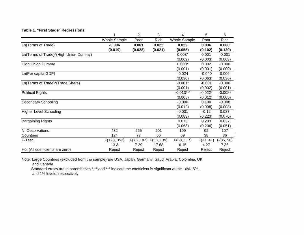
Table 1. "First Stage" Regressions1 2 3 4 5 6

Whole Sample Poor Rich Whole Sample Poor RichLn(Terms of Trade) -0.006 0.001 0.022 0.022 0.036 0.080

(0.019) (0.028) (0.021) (0.055) (0.102) (0.120)Ln(Terms of Trade)*(High Union Dummy) 0.003* 0.001 -0.001

(0.002) (0.003) (0.003)High Union Dummy 0.000* 0.002 -0.000

(0.001) (0.001) (0.000)Ln(Per capita GDP) -0.024 -0.040 0.006

(0.030) (0.063) (0.036)Ln(Terms of Trade)*(Trade Share) -0.001* -0.001 -0.000

(0.001) (0.002) (0.001)Political Rights -0.013*** -0.022* -0.008*

(0.005) (0.012) (0.005)Secondary Schooling -0.000 0.100 -0.008

(0.012) (0.098) (0.008)Higher Level Schooling -0.001 -0.12 0.037

(0.083) (0.223) (0.070)Bargaining Rights 0.073 0.293 0.037

(0.068) (0.206) (0.051)N. Observations 482 265 201 199 92 107Countries 124 77 56 69 38 36F-Test F(123, 352) F(76, 182) F(55, 139) F(68, 117) F(37, 41) F(35, 58)

13.3 7.29 17.68 6.15 4.27 7.36H0: (All coefficients are zero) Reject Reject Reject Reject Reject Reject

Note: Large Countries (excluded from the sample) are USA, Japan, Germany, Saudi Arabia, Colombia, UK and Canada Standard errors are in parentheses.*,** and *** indicate the coefficient is significant at the 10%, 5%, and 1% levels, respectively

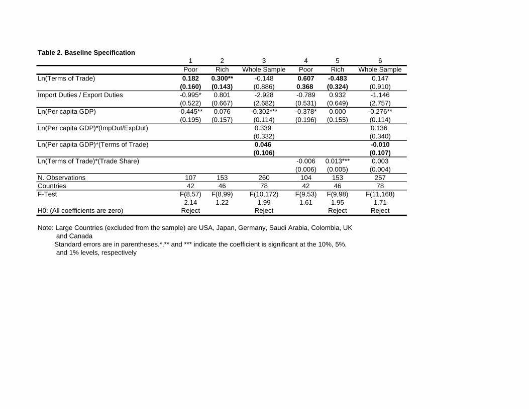
Table 2. Baseline Specification1 2 3 4 5 6

Poor Rich Whole Sample Poor Rich Whole SampleLn(Terms of Trade) 0.182 0.300** -0.148 0.607 -0.483 0.147

(0.160) (0.143) (0.886) 0.368 (0.324) (0.910)Import Duties / Export Duties -0.995* 0.801 -2.928 -0.789 0.932 -1.146

(0.522) (0.667) (2.682) (0.531) (0.649) (2.757)Ln(Per capita GDP) -0.445** 0.076 -0.302*** -0.378* 0.000 -0.276**

(0.195) (0.157) (0.114) (0.196) (0.155) (0.114)Ln(Per capita GDP)*(ImpDut/ExpDut) 0.339 0.136

(0.332) (0.340)Ln(Per capita GDP)*(Terms of Trade) 0.046 -0.010

(0.106) (0.107)Ln(Terms of Trade)*(Trade Share) -0.006 0.013*** 0.003

(0.006) (0.005) (0.004)N. Observations 107 153 260 104 153 257Countries 42 46 78 42 46 78F-Test F(8,57) F(8,99) F(10,172) F(9,53) F(9,98) F(11,168)

2.14 1.22 1.99 1.61 1.95 1.71H0: (All coefficients are zero) Reject Reject Reject Reject


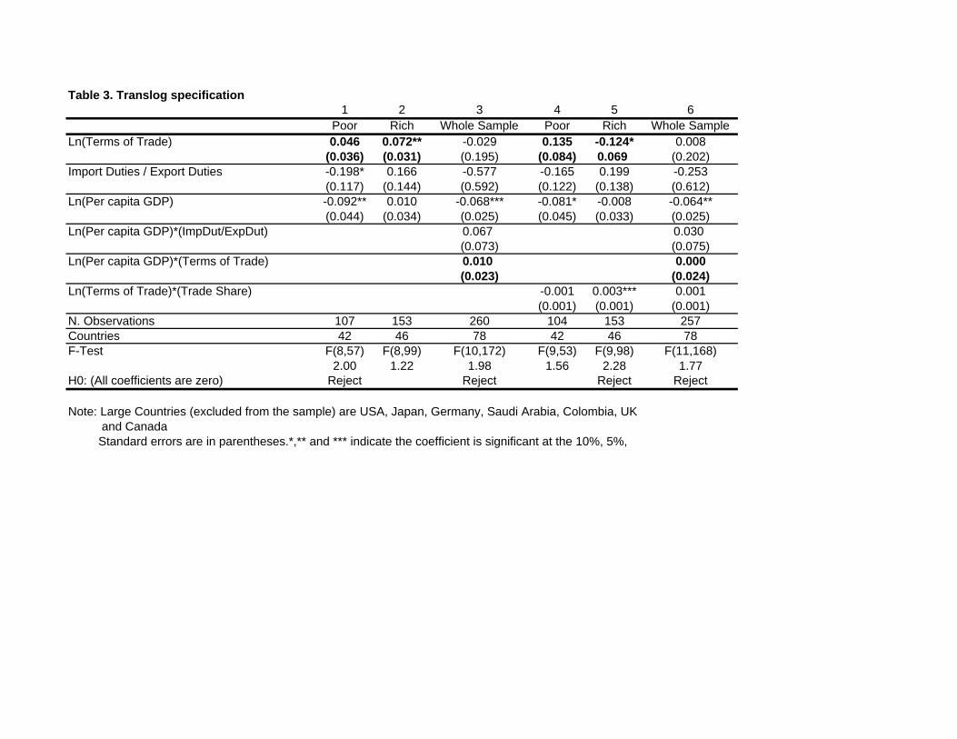
Table 3. Translog specification1 2 3 4 5 6

Poor Rich Whole Sample Poor Rich Whole SampleLn(Terms of Trade) 0.046 0.072** -0.029 0.135 -0.124* 0.008

(0.036) (0.031) (0.195) (0.084) 0.069 (0.202)Import Duties / Export Duties -0.198* 0.166 -0.577 -0.165 0.199 -0.253

(0.117) (0.144) (0.592) (0.122) (0.138) (0.612)Ln(Per capita GDP) -0.092** 0.010 -0.068*** -0.081* -0.008 -0.064**


(0.073) (0.075)Ln(Per capita GDP)*(Terms of Trade) 0.010 0.000

(0.023) (0.024)Ln(Terms of Trade)*(Trade Share) -0.001 0.003*** 0.001


2.00 1.22 1.98 1.56 2.28 1.77H0: (All coefficients are zero) Reject Reject Reject Reject

Note: Large Countries (excluded from the sample) are USA, Japan, Germany, Saudi Arabia, Colombia, UK and Canada Standard errors are in parentheses.*,** and *** indicate the coefficient is significant at the 10%, 5%,

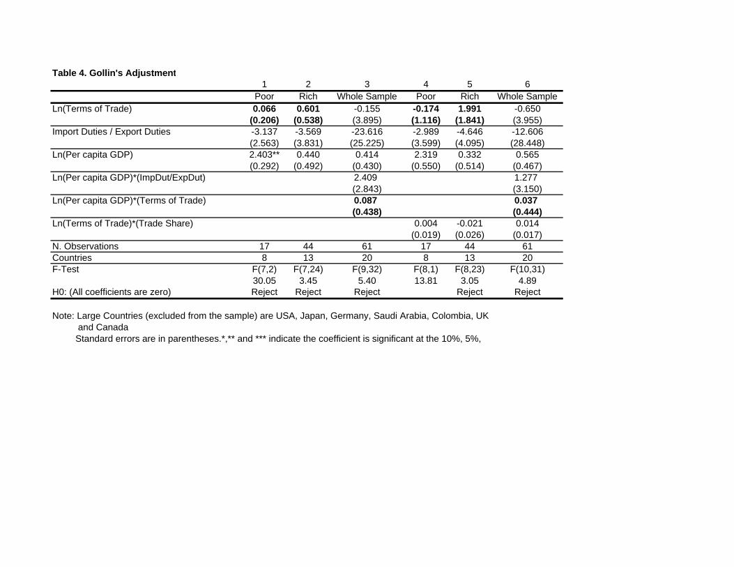
Table 4. Gollin's Adjustment1 2 3 4 5 6

Poor Rich Whole Sample Poor Rich Whole SampleLn(Terms of Trade) 0.066 0.601 -0.155 -0.174 1.991 -0.650

(0.206) (0.538) (3.895) (1.116) (1.841) (3.955)Import Duties / Export Duties -3.137 -3.569 -23.616 -2.989 -4.646 -12.606

(2.563) (3.831) (25.225) (3.599) (4.095) (28.448)Ln(Per capita GDP) 2.403** 0.440 0.414 2.319 0.332 0.565


(2.843) (3.150)Ln(Per capita GDP)*(Terms of Trade) 0.087 0.037

(0.438) (0.444)Ln(Terms of Trade)*(Trade Share) 0.004 -0.021 0.014


30.05 3.45 5.40 13.81 3.05 4.89H0: (All coefficients are zero) Reject Reject Reject Reject Reject

Note: Large Countries (excluded from the sample) are USA, Japan, Germany, Saudi Arabia, Colombia, UK and Canada Standard errors are in parentheses.*,** and *** indicate the coefficient is significant at the 10%, 5%,

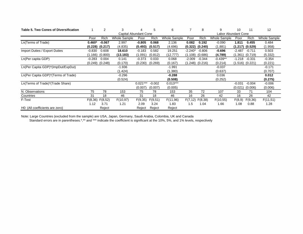
Table 5. Two Cones of Diversification 1 2 3 4 5 6 7 8 9 10 11 12

Poor Rich Whole Sample Poor Rich Whole Sample Poor Rich Whole Sample Poor Rich Whole SampleLn(Terms of Trade) 0.460* -0.067 2.997 -0.805 0.068 2.136 0.082 0.192 -0.090 1.811 0.455 0.484

(0.228) (0.217) (4.835) (0.493) (0.517) (4.696) (0.322) (0.240) (1.881) (1.217) (0.529) (1.958)Import Duties / Export Duties -0.830 0.608 18.610 -0.183 0.582 19.251 -2.240* -0.806 -0.696 -2.487 -0.711 0.503

(1.166) (0.800) (13.183) (1.091) (0.812) (12.777) (1.108) (0.686) (4.789) (1.361) (0.719) (5.332)Ln(Per capita GDP) -0.283 0.004 0.141 -0.373 0.033 0.068 -2.009 -0.344 -0.439** -1.218 -0.331 -0.354

(0.249) (0.248) (0.170) (0.230) (0.269) (0.167) (1.248) (0.216) (0.214) (1.516) (0.221) (0.221)Ln(Per Capita GDP)*(ImpDut/ExpDut) -1.936 -1.991 -0.037 -0.171

(1.424) (1.380) (0.637) (0.707)Ln(Per Capita GDP)*(Terms of Trade) -0.296 -0.288 0.036 0.012

(0.524) (0.508) (0.252) (0.275)Ln(Terms of Trade)*(Trade Share) 0.021*** -0.002 0.013*** -0.031 -0.004 -0.006

(0.007) (0.007) (0.005) (0.021) (0.006) (0.006)N. Observations 75 78 153 75 78 153 35 72 107 33 71 104Countries 31 18 46 31 18 46 16 26 42 16 26 42F-Test F(8,36) F(8,52) F(10,97) F(9,35) F(9,51) F(11,96) F(7,12) F(8,38) F(10,55) F(8,9) F(9,36) F(11,51)

1.12 3.71 1.21 2.09 3.24 1.83 1.5 1.04 1.66 1.08 0.88 1.28H0: (All coefficients are zero) Reject Reject Reject Reject


Capital Abundant Cone Labor Abundant Cone

Table 6. Alternative specifications1 2 3 4 5 6

Poor Rich Whole Sample Poor Rich Whole SampleLn(Terms of Trade) -0.484 -0.053 -0.007

(0.505) (0.501) (0.844)Import Duties / Export Duties -0.413 1.373* -6.961*** -1.367 0.465 -2.046

(0.705) (0.719) (2.454) (0.921) (0.947) (5.628)Ln(Per capita GDP) -0.994*** 0.327 -0.505*** -0.459 0.030 -0.486*

(0.292) (0.299) (0.192) (0.405) (0.442) (0.288)Ln(Capital per Worker) 0.348 -0.097 -0.061

(0.274) (0.248) (0.187)Ln(Terms of Trade)*(Trade Share) 0.014 0.004 0.010*

(0.009) (0.010) (0.282)Ln(Capital per Worker)*(Imp.Dut/Exp.Dut) 0.813***

(0.087)Ln(Capital per Worker)*(Terms of Trade) -0.051

(0.006)Ln(Per capita GDP)*(Terms of Trade)

Ln(Terms of Trade Barro-Lee) 3.941 -1.247 6.882(2.963) (2.037) (7.793)

Ln(Terms of Trade Barro-Lee)*(Trade Share) -0.057 0.010 -0.008(0.044) (0.020) (0.017)

Ln(Per capita GDP)*(Terms of Trade Barro-Lee) -0.658(0.936)

Ln(Per capita GDP)*(Imp.Dut/Exp.Dut) 0.177(0.671)

Trade Share

Ln(Per capita GDP)*(Trade Share)

Political Rights

Secondary Schooling

Higher Level Schooling

Bargaining Rights

N. Observations 64 86 150 53 57 110Countries 20 21 38 33 30 59F-Test F(19, 35) F(20, 56) F(37, 101) F(32, 14) F(29, 21) F(58, 43)



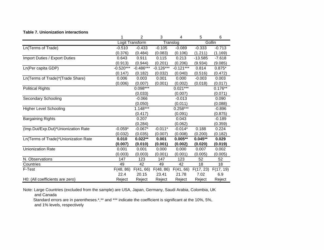
Table 7. Unionization interactions1 2 3 4 5 6

Ln(Terms of Trade) -0.510 -0.433 -0.105 -0.089 -0.333 -0.713(0.376) (0.484) (0.083) (0.106) (1.211) (1.169)

Import Duties / Export Duties 0.643 0.911 0.115 0.213 -13.585 -7.618(0.913) (0.944) (0.201) (0.206) (9.934) (9.085)

Ln(Per capita GDP) -0.520*** -0.486*** -0.126*** -0.121*** 0.814 0.875*(0.147) (0.182) (0.032) (0.040) (0.516) (0.472)

Ln(Terms of Trade)*(Trade Share) 0.006 0.003 0.001 0.000 -0.003 0.003(0.006) (0.007) (0.001) (0.002) (0.018) (0.017)

Political Rights 0.098*** 0.021*** 0.176**(0.033) (0.007) (0.071)

Secondary Schooling -0.066 -0.013 0.090(0.050) (0.011) (0.088)

Higher Level Schooling 1.148*** 0.258*** -0.896(0.417) (0.091) (0.875)

Bargaining Rights 0.207 0.043 -0.189(0.284) (0.062) (0.359)

(Imp.Dut/Exp.Dut)*Unionization Rate -0.059* -0.067* -0.011* -0.014* 0.188 0.224(0.032) (0.035) (0.007) (0.008) (0.200) (0.182)

Ln(Terms of Trade)*Unionization Rate 0.010 0.022** 0.001 0.005** 0.045** 0.029(0.007) (0.010) (0.001) (0.002) (0.020) (0.019)

Unionization Rate 0.001 0.001 0.000 0.000 0.007 0.002(0.003) (0.003) (0.001) (0.001) (0.005) (0.005)

N. Observations 147 123 147 123 52 52Countries 49 42 49 42 18 18F-Test F(48, 86) F(41, 66) F(48, 86) F(41, 66) F(17, 23) F(17, 19)



GollinLogit Transform Translog

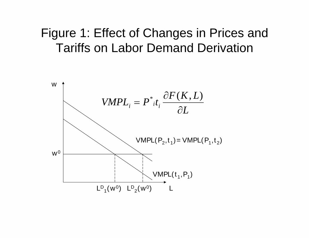
Figure 1: Effect of Changes in Prices andTariffs on Labor Demand Derivation

VMPL(t1,P1)

VMPL(P2,t1)=VMPL(P1,t2)

w0

LD1(w0) LD

2(w0) L

w

LLKFtPVMPL iii ∂

∂=

),(*

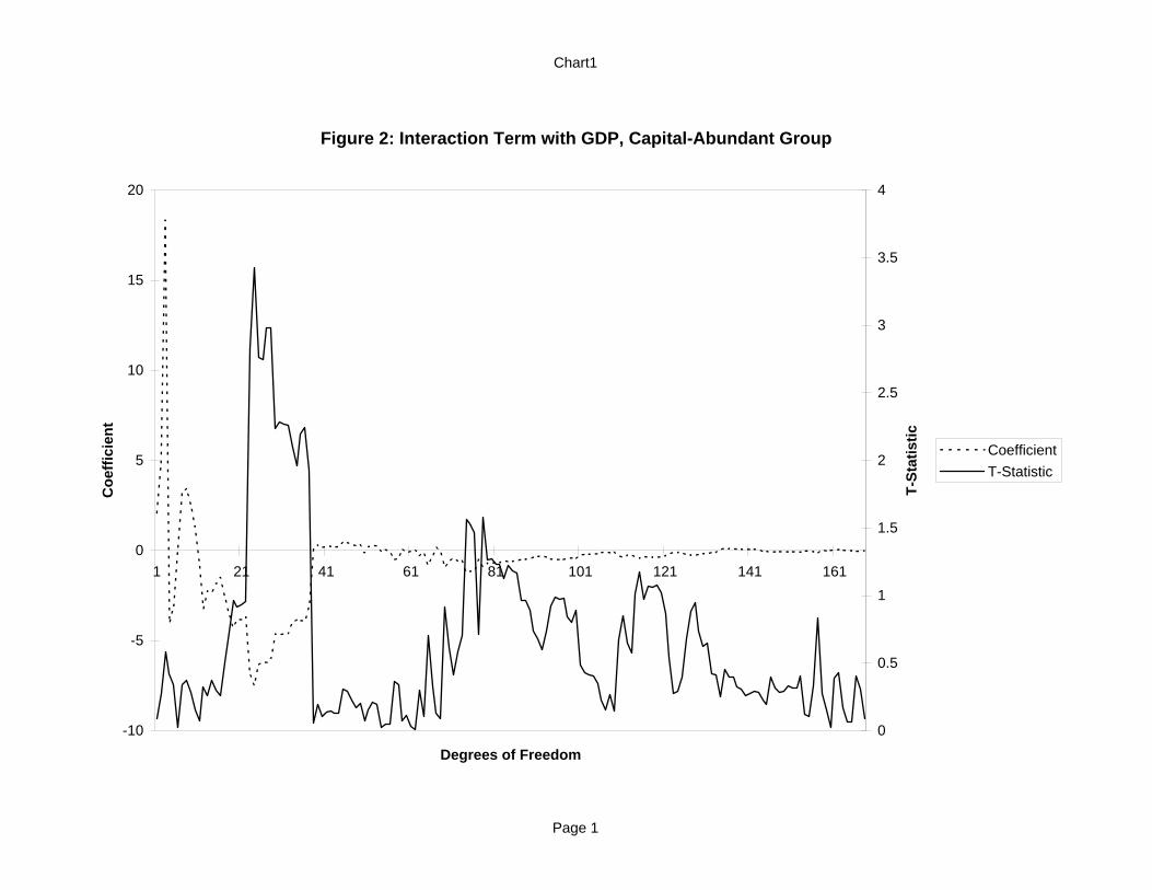
Chart1

Page 1

Figure 2: Interaction Term with GDP, Capital-Abundant Group

-10

-5

0

5

10

15

20

1 21 41 61 81 101 121 141 161

Degrees of Freedom

Coe

ffici

ent

0

0.5

1

1.5

2

2.5

3

3.5

4

T-St

atis

tic

CoefficientT-Statistic

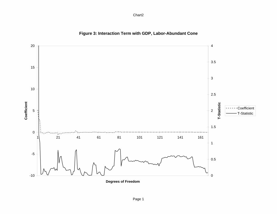
Chart2

Page 1

Figure 3: Interaction Term with GDP, Labor-Abundant Cone

-10

-5

0

5

10

15

20

1 21 41 61 81 101 121 141 161

Degrees of Freedom

Coe

ffici

ent

0

0.5

1

1.5

2

2.5

3

3.5

4

T-St

atis

tic

CoefficientT-Statistic

trade policy and factor prices: an empirical...

Documents