trade, growth, and the environment nexus: the experience
TRANSCRIPT

University of Wollongong Thesis Collections
University of Wollongong Thesis Collection
University of Wollongong Year
Trade, growth, and the environment
nexus: the experience of China,
1990-2007
Ying LiuUniversity of Wollongong
Liu, Ying, Trade, growth, and the environment nexus: the experience of China, 1990-2007, Master of Economics by Research thesis, School of Economics, Faculty of Commerce,University of Wollongong, 2009. http://ro.uow.edu.au/theses/3040
This paper is posted at Research Online.


Trade, Growth, and the Environment Nexus: The Experience of China, 1990-2007
A thesis is submitted in fulfilment of the requirements for the award of the degree
Master of Economics by Research
from
University of Wollongong
by
Ying Liu
Bachelor of Economics (Nanjing Audit Institute, China) Master of Professional Accounting (University of Wollongong, Australia)
School of Economics Faulty of Commerce
University of Wollongong, Australia, 2009

CERTIFICATION
I, Ying Liu, declare that this thesis, submitted in fulfilment of the requirements for the
award of Master of Economics by Research, in the department of Economics,
University of Wollongong, is wholly my own work unless otherwise referenced or
acknowledged. The document has not been submitted for qualifications at any other
academic institution.
Ying Liu
10 August 2009

i
TABLE OF CONTENTS
List of Tables………………………………………………………………………...iv
List of Figures………………………………………………………………………..vi
Abbreviations……………………………………………………………………….vii
Abstract………………………………………………………………………………ix
Acknowledgements…………………………………………………………………x
CHAPTER ONE: INTRODUCTION
1.1 Background of the Study………………………………………………………...1
1.2 Research Methodology…………………………………………………………..2
1.2.1 Objective and Hypotheses…………………………………………………...2
1.2.2 Methodology ………………………………………………………………..2
1.2.3 Data …………………………………………………………………………3
1.3 Significance of the Research ……………………………………………………4
1.4 Sequence of Chapters …………………………………………………………...5
CHAPTER TWO: A SURVEY OF LITERATURE
2.1 Background………………………………………………………………………6
2.2 Theoretical Perspective………………………………………………………….6
2.3 Empirical Evidence……………………………………………………………..10
2.3.1 Environmental Kuznets Curve (EKC)……………………………………..10
2.3.2 Trade and the Environment………………………………………………..16
2.3.3 Computable General Equilibrium (CGE) Models…………………………22
2.4 Conclusion………………………………………………………………………23
CHAPTER THREE: THE ECONOMY OF CHINA
3.1 General Background……………………………………………………………25
3.2 China’s Reforms………………………………………………………………...26
3.2.1 Pre-reform: 1949-1978………………………………………………26
3.2.2 Post-reform: 1979-Present…………………………………………..27
3.2.2.1 Rural Economic Reform…………………………………………27

ii
3.2.2.2 Enterprise Reform: SOEs and Non-SOEs………………………28
3.2.2.3 Trade Reform………………………………………………………31
3.2.2.4 Foreign Direct Investment Reform……………………………….33
3.3 Performance…………………………………………………………………….35
3.3.1 Economic Growth and Structural Change…………………………………35
3.3.2 The Development of Foreign Trade………………………………………..37
3.4 Conclusion………………………………………………………………………39
CHAPTER FOUR: ECONOMIC GROWTH AND THE ENVIRONMENT
IN CHINA
4.1 Introduction……………………………………………………………………..41
4.2 China’s Economic Development Phases and Environmental Problems…….42
4.2.1 Early Stage (1949-1978)…………………………………………………...42
4.2.2 Initial Emergence of Environmental Problems (1978-1984)………………43
4.2.3 Emergence of Environmental Problems (1985-1992)……………………..43
4.2.4 Increasingly Serious Environmental Problems (1993-1999)………………44
4.2.5 Intensive Outburst of Environmental Problems (2000 to now)……………44
4.3 Legislation on Environmental Standards……………………………………..47
4.4 Empirical Review: China………………………………………………………50
4.5 Empirical Methodology and Data……………………………………………..55
4.5.1 Empirical Methodology……………………………………………………55
4.5.2 Summary Statistics…………………………………………………………58
4.6 Empirical Results……………………………………………………………….59
4.6.1 Whole Country……………………………………………………………..60
4.6.2 Coastal Region……………………………………………………………62
4.6.3 Central Region……………………………………………………………..64
4.6.4 Western Region…………………………………………………………….66
4.7 Conclusion………………………………………………………………………67
CHAPTER FIVE: TRADE LIBERALISATION AND THE ENVIRONMENT:
Evidence from China’s Industrial Sector
5.1 Introduction……………………………………………………………………..70
5.2 The Relationship between Trade and the Environment……………………..70

iii
5.3 Literature Review: China………………………………………………………73
5.4 Model Specification and Data Description……………………………………77
5.4.1 Model Specification………………………………………………………..77
5.4.1.1 Income Equation…………………………………………………...78
5.4.1.2 Emission Equation…………………………………………………80
5.4.1.3 Econometrics Framework………………………………………….81
5.4.2 Data Description…………………………………………………………...84
5.5 Empirical Estimation…………………………………………………………...86
5.5.1 Estimation Technique……………………………………………………...86
5.5.2 Results of Estimation………………………………………………………88
5.5.2.1 Full Sample………………………………………………………...93
5.5.2.2 Sub-Samples……………………………………………………...95
5.5.2.3 The Net Trade Liberalisation Impact…………………………….96
5.6 Conclusion……………………………………………………………………..97
CHAPTER SIX: SUMMARY AND RECOMMENDATIONS
6.1 Summary………………………………………………………………………99
6.2 Major Findings………………………………………………………………..101
6.3 Policy Recommendations……………………………………………………..103
6.4 Limitations and Future Studies………………………………………………103
REFERENCES…………………………………………………………………..105

iv
LIST OF TABLES
Table 2.1: Summary of EKC Empirical Analysis……………………………………14
Table 2.2: Pro-Environment and Pro-Trade Arguments……………………………..16
Table 2.3 Summary of Estimations on the Impact of
Trade Liberalisation on Pollution…………………………………………21
Table 3.1: TVE Employment by Ownership, 2003………………………………….28
Table 3.2: Ownership of Industrial Output (1978-1996)…………………………….30
Table 3.3: Ownership of Industrial Output (above-scale industry)
(1998-2007)………………………………………………………………30
Table 3.4: Major Foreign Investors in China: 1979-2007…………………………...34
Table 3.5: FDI by Sectors in 2007…………………………………………………...35
Table 3.6: Growth of GDP…………………………………………………………...36
Table 3.7: Composition of China’s Exports and Imports……………………………38
Table 3.8: China’s Major Trading Partners, 2007………………………………….39
Table 4.1: Water Quality of Major Lakes and Reservoirs, 2007…………………….47
Table 4.2: EKC Empirical Analyses for China………………………………………53
Table 4.3 Types of Relationship between Environmental Quality and
Economic Growth………………………………………………………...56
Table 4.4: Region Definitions………………………………………………………..57
Table 4.5: Summary Statistics, 1990-2007…………………………………………..58
Table 4.6: Estimates for 30 Provinces……………………………………………….60
Table 4.7: Estimates for Provinces in the Coastal Region…………………………..62
Table 4.8: Estimates for Provinces in the Central Region…………………………...64
Table 4.9: Estimates for Provinces in the Western Region………………………….66
Table 5.1: Summary of Estimations on the Impact of Trade
Liberalisation on the Environment………………………………………77
Table 5.2: Expected Signs for the Estimated Coefficients in
Equ. (10) and (11)………………………………………………………..84
Table 5.3: Summary Statistics of Variables…………………………………………86

v
Table 5.4: Correlation Coefficients…………………………………………………..89
Table 5.5: Regression Diagnostics…………………………………………………...90
Table 5.6: Estimated Results for Equation (11)……………………………………...91
Table 5.7: Estimated Results for Equation (10)……………………………………...92
Table 5.8: Chow-Test Results………………………………………………………95
Table 5.9: The Net Trade Liberalisation Impact on
Pollutants Emissions……………………………………………………97

vi
LIST OF FIGURES
Figure 2.1: The Environmental Kuznets Curves (EKC)………………………………9
Figure 3.1: Annual Utilised FDI, 1979-2007 ($ billion)……………………………..34
Figure 3.2: Annual GDP Growth, 1978-2007……………………………………….36
Figure 3.3: Composition of GDP……………………………………………………36
Figure 3.4: Growth of China’s Foreign Trade ($ 100 million)………………………38
Figure 3.5: Trade Dependence Ratio (% of GDP)…………………………………...38
Figure 3.6: Foreign Exchange Reserves ($ 100 billion)……………………………..39
Figure 4.1: Urban Air Quality……………………………………………………….46
Figure 4.2: Water Quality Comparison of the Seven Major Rivers…………………47
Figure 4.3: Per Capita Emissions in China: 1990-2007……………………………..59
Figure 4.4: The EKC for SO2: Whole Country (Quadratic Form)…………………..61
Figure 4.5: The EKC for SO2: Coastal Region (Cubic Form)………………………63
Figure 4.6: The EKC for Smoke: Coastal Region (Cubic Form)……………………63
Figure 4.7: The EKC for SO2: Central Region (Cubic Form)……………………...65
Figure 4.8: The EKC for Dust: Central Region (Cubic Form)……………………..65
Figure 4.9: The EKC for COD: Western Region (Cubic Form)……………………67
Figure 6.1: Per Capita Emissions in China, 1990-2007…………………………….100

vii
ABBREVIATIONS
APEC Asia-Pacific Economic Cooperation
ASEAN Association of Southeast Asian Nations
BOD Biochemical Oxygen Demand
CEECs Central and Eastern European Countries
CGE Computable General Equilibrium
CO Carbon Monoxide
CO2 Carbon Dioxide
COD Chemical Oxygen Demand
CPC Communist Party of China
CPI Consumer Price Index
DO Dissolved Oxygen
EIA Environmental Impact Assessment
EKC Environmental Kuznets Curve
EP Export Processing
EPBs Environmental Protection Bureaus
EPOs Environmental Protection Offices
ERPC Environmental and Resources Protection Committee
ETDZs Economic and Technological Development Zones
EU European Union
FDI Foreign Direct Investment
FYP Five-Year Plan
GDP Gross Domestic Production
GEMS Global Environmental Monitoring System
GLF Great Leap Forward
HO Heckscher-Ohlin
MEP Ministry of Environmental Protection
MERCOSUR Common Market of the Southern Cone
NAFTA North American Free Trade Agreement
NEPA National Environmental Protection Agency
NOX Nitrogen Oxides
viii
NPC National People's Congress
ODI Outward Direct Investment
OECD Organisation for Economic Cooperation and Development
OLS Ordinary Least Squares
PIM Perpetual Inventory Method
PPP Purchasing Power Parity
PRC People's Republic of China
SEPA State Environmental Protection Agency
SEPC State Environmental Protection Commission
SEZs Special Economic Zones
SO Sulphur Monoxide
SO2 Sulphur Dioxide
SOEs State-owned Industrial Enterprises
SPM Suspended Particulate Matter
TOT Terms of Trade
TVEs Township and Village Enterprises
UK United Kingdom
USA United States of America
UN United Nations
UNCHE United Nations Conference on the Human Environment
VAT Value-added Taxes
WTO World Trade Organisation
2SLS Two-Stage Least Squares
ix
ABSTRACT
The market-oriented economic reforms that started in 1978 have greatly transformed the Chinese economy. China’s GDP has increased tenfold since 1978 while the per capita income has grown at an average annual rate of more than 8% over the last three decades, drastically reducing poverty. China’s foreign trade has grown faster than its GDP for the past 25 years (Chen and Li, 2000). Although industrial emissions increased in absolute terms that has been a noticeable reduction in per capita emissions especially after 1997. The major objective of this thesis is to study the nexus of trade, economic growth, and the environment in China during the period from 1990 to 2007. There are two interrelated hypotheses to be tested for this purpose: (1) The Environmental Kuznets Curve (EKC) hypothesis and (2) Trade liberalisation in China had a short term negative effect on the environment and a long term positive effect based on the assumption that externality can be internalised and that an EKC exists in China. Both quadratic and cubic EKC models were used to capture the relationship between the per capita of income and the per capita of four industrial pollution emissions (SO2, smoke, dust, and COD). Due to an unbalanced development among the regions, this study grouped the whole country into three regions to examine the impact of a geographic location. The fixed effect and panel data were used. The results showed that an inverted-U shaped relationship as hypothesised by the EKC quadratic model in the case of SO2 exists, with a turning point at per capita GDP of 6,376 yuan, while N-shaped curves were found for smoke, dust and COD in different regions. The results also showed that the more developed coastal region appears to have a turning point at a higher income level than the less developed central and western regions. To study the impact of trade liberalisation on the environment, this study adopted a modified version of Dean’s (2002) simultaneous model using a disaggregated sample based on above and below the turning point of the EKC. The Two-Stage Least Squares method was used. The results from the overall sample showed that the scale effects outweighed the technique effects for air pollutant (SO2) and water pollutant (COD), which is evidence for the pollution haven hypothesis. The split sample provided limited support for the EKC hypothesis where a rising level of income at the provincial level via an increased level of international trade was associated with falling emissions from the technique effect, so that rising income among the provinces tended to show a superior performance. In order to harmonise development stricter environmental regulations must be associated with growing incomes because they may provide the motivation for better production techniques.

x
ACKNOWLEDGEMENTS
The completion of this thesis has involved many people to whom I would like to thank for their help and encouragement during my studies. I wish to express my sincere appreciation and gratitude to Dr. Kankesu Jayanthakumaran, my supervisor, who has provided timely, energetic and instructive comments and evaluation at every stage of the dissertation process. My special thanks are given to Miss Yuqing Zhu, who has spent lots of time to help and teach me the statistical software of STATA that can be used to analyse the panel data. In particular, I wish to recognize the impact of my mother and my father, have had on my life. They instilled in me the importance of obtaining a good education, and exhibiting perseverance. And their continued moral support, help and encouragement for all these years are very much appreciated.

1
CHAPTER ONE
INTRODUCTION
1.1 Background of the Study
In the early 1990s there were two significant events that dramatically affected the
whole world. One was the establishment of the World Trade Organisation (WTO) in
1994 based on the belief that trade liberalisation would enhance world economic
welfare. The other was the concept of sustainable development that arose from the
United Nations Conference on Environment and Development in 1992 where this
concept was stressed in the Rio Declaration. Environmental protection has become an
exceedingly important objective and as time has passed the massive wave of trade
liberalisation that has continued since the last decade has generated an interesting and
contentious debate in terms of its impact on the environment.
In recent years a large volume of literature regarding the links between trade,
economic growth, and the environment has been generated. By taking a lead from
earlier work on economic growth and the environment (Grossman and Krueger 1991),
the environmental effects of trade can be analytically separated into three
components1: scale, technique, and composition effects. A negative scale effect has
the potential to encourage short-term growth at the cost of hampering long-term
economic development by causing irreversible damage to the environment.
Environmentalists argue that a negative composition effect that complements the
scale effect exacerbates the degradation of natural resources in developing countries.
However, the proponents of free trade argue that trade liberalisation leads to positive
technique and composition effects via income growth, which potentially outweigh the
negative scale effect.
The contradictory predictions of both schools of thought and the mixed empirical
evidence2 suggest that trade liberalisation is a double-edged sword presenting both
threats and opportunities to the environment. Earlier research has largely been
confined to cross-country investigations that were sensitive to the choice of pollutants 1 This point is discussed in details in Chapter Two. 2 The detailed discussion of past empirical studies is undertaken in Chapter Two.
2
and the countries included in the sample. Vincent (1997) and Stern et al. (1994)
argued that the cross-country investigations into the relationship between economic
growth and pollution have been unhelpful in offering guidance and sound policy
advice to the developing countries. In recent years an increased emphasis has been
placed on examining the experience of individual countries so that policy frameworks
are suggested according to their unique circumstances and resources.
In China there has been considerable research into the impact of trade liberalisation
on the environment. Like many other developing countries, China first commenced
rapid liberalisation from the early 1990s onwards but has also experienced a rise in
pollution during the last two decades. It is therefore important to discover whether
increased trade activity has played a role in the deterioration of the environment but
unfortunately there are very few studies on this topic. Dean (2002), Chai (2002), Shen
(2008), and Dean and Lovely (2008) have all tried to find out whether trade
liberalisation harmed China’s environment, but the results are ambiguous due to the
methodologies used, the time period, and the environmental indicators.
1.2 Research Methodology
1.2.1 Objective and Hypotheses
The main objective of this research is to examine the relationship between trade
liberalisation, economic growth, and the environment in China during the period
1990-2007. There are two interrelated hypotheses to be tested for this purpose:
(1) The Environmental Kuznets Curve (EKC) hypothesis;
(2) Trade liberalisation has a short term negative effect on the environment but the
long term positive effect will occur provided that externalities can be internalised
with a rise in income and the introduction of new technology.
1.2.2 Methodology
Different methodologies will be used to achieve this objective. To test hypothesis (1),
the author will use both quadratic and cubic Environmental Kuznets Curve (EKC)
models, following Cole et al. (1997), Dinda et al. (2000), Cole and Elliott (2003), and
Llorca and Meunie (2009). An estimation of the EKC will be done using panel

3
regression based on the data for 30 Chinese provinces from 1990 to 2007. Due to a
large disparity in growth among the regions, it is worth while to explore whether the
relationship between income and pollution varies by region. All provinces are
considered as a whole or grouped into coastal, central, and western regions.
To test hypothesis (2), a simultaneous equations system developed by Dean (2002),
which incorporates the multiple effects of trade liberalisation on the environment, will
be used on pooled Chinese provincial data from 1990 to 2007. The whole sample will
be split into two sub-samples based on the turning point of EKC, income per capita
above and below 6,500 yuan.
1.2.3 Data
This research uses a provincial dataset from the China Statistical Yearbook and the
China Environmental Statistical Yearbook of air and water pollution from 1990 to
2007. This dataset is advantageous for several reasons. Dean (2002) argued that the
developing country chosen for analysis must have the following, lengthy time series
data available on environmental damage, regulations which internalise environmental
externalities, undertaken trade reforms, and experienced large increases in
international trade volume during that period. China is one of the few developing
countries that have had an extensive air and water pollution levy system in place for
many years. China also undertook extensive trade reforms during 1990-2007 which
resulted in a huge increase in international trade. In addition, 18 years of data pooled
across the provinces should yield a closer approximation to the experience of one
developing country.
In this research our interest is in China’s trade, growth, and the environment rather
than the global environment. Hence, we focus on the primary pollutants which China
uses to evaluate its own environment rather than the greenhouse gases associated with
global climate change. In the 11th Five-Year Plan (FYP) (2006-2010), the Chinese
government stated explicit goals for reducing its water pollution, as measured by the
Chemical Oxygen Demand (COD) and air pollution, as measured by the Sulphur

4
Dioxide (SO2) and particulate matter (especially that generated by Smoke and Dust)3.
COD measures the mass concentration of oxygen consumed by the chemical
breakdown of organic and inorganic matter in water.4 COD emissions account for the
majority of industrial water pollution levies collected during this period. While the
emissions from other water pollutants were recoded in more recent years, they are
generally positively correlated with COD (Dean and Lovely, 2008). The industrial
SO2 emissions include the sulphur dioxide emitted from fuel burning and the
production processes on the premises of an enterprise. Industrial Smoke emissions
include the smoke emitted from fuel burning on the premises of an enterprise.
Industrial Dust emissions refer to the volume of dust suspended in the air and emitted
by the productive processes of an enterprise.5
1.3 Significance of the Research
As noted earlier, past researchers have not generated uniform results about the trade-
growth-environment relationship in different countries or an individual country, so
whether an increased level of trade increases pressures on the environment is the
centre of much ongoing debate. Further research is needed in order to shed light on
the impact of trade and economic growth on the environment. From the early 1990s
China has experienced rapid trade liberalisation and environmental degradation so a
study of the linkage between trade liberalisation, growth, and the environment would
be important and apposite. This study will discover whether liberalising trade and
growing economics will harm the environment or not.
This thesis will examine the impact of trade and growth on the environment in China
as a whole, using 18 years provincial level data. It will also examine the effect of
trade and growth on a geographic location by grouping 30 provinces into three
regions. It will then split the whole sample into higher and lower levels of income in
order to examine the impact of the per capita income differentials.
3 The National 11th Five Year Plan for Environmental Protection (2006-2010). 4 China Statistical Yearbook on Environment, 2006, p.207. 5 China Statistical Yearbook on Environment, 2006, p.208.

5
The results of this research will definitely throw light on the relationship between
trade, growth, and the environment. These results will also be important for China
and be of interest to policy-makers as a guide for future trade policy formulation.
1.4 Sequence of Chapters
This thesis is divided into six chapters. Chapter Two is a literature review that
focussed on recent studies that considered the link between trade, growth and the
environment and presented methodologies and results from different empirical studies.
Chapter Three gives a picture of China’s general background, economic reforms, and
performance by examining how the Chinese economic structure has changed from the
1950s to the present time.
In Chapter Four the relationship between China’s economic growth and
environmental pollution from 1990 to 2007 is studied. We will use EKC models to
examine whether economic growth eventually brings environmental improvement
and if so, where is the turning point in China.
The focus in Chapter Five is on the impact of trade liberalisation on the environment.
A simultaneous equations system will be used to capture the effect of trade
liberalisation on environmental pollution through direct impact via the composition
effect, and indirect impact via the scale and technique effects.
The last chapter presents a summary of the major findings from previous studies and
ends with some limitations and recommendations for future study.
6
CHAPTER TWO
A SURVEY OF LITERATURE
2.1 Background
A policy of trade liberalisation is often suggested as a means of stimulating economic
growth in developing countries. Trade liberalisation consists of policies aimed at
opening up the economy to foreign investment and lowering trade barriers in the form
of tariff reduction. However, while trade may stimulate growth, it may
simultaneously lead to more pollution either as a result of the relocation of polluting
industries from countries with strict environmental regulation, or owing to increased
production in dirty industries (Mukhopadhyay and Chakraborty, 2005). Given its
potential benefits it is important to examine whether trade opening conflicts with the
environment as production is expanded and economic growth accelerates.
What happens to the environment when international trade is liberalised is a matter of
debate. The literature on the effects of free trade on the environment has been
increasing (For example, Grossman and Krueger, 1991, 1995; Shafik and
Bandyopadhyay, 1992; Selden and Song, 1994; Beghin et al., 1995, 2002; Panayotou,
1997; Antweiler et al, 2001; Dean, 2002; Frankel and Rose, 2002; Cole and Elliot,
2003; Cole, 2004; Copeland and Taylor, 2004). The methodologies used to test these
relationships vary widely, as do the results. In this chapter, literature pertaining to the
connection between trade, income, and the environment, will be reviewed.
The rest of this chapter is organised as follows: section 2.2 outlines the theoretical
perspective, section 2.3 reports the empirical studies of EKC, trade-environment, and
CGE models, and section 2.4 concludes.
2.2 Theoretical Perspective
The issue of whether increased levels of trade will lead to increased pressure on the
environment has fuelled much of the ongoing trade-environment debate. A pollution
haven hypothesis suggests that liberalising trade would cause ‘dirty industries’ to
migrate from developed countries to developing countries. In the developing

7
countries, economic growth and improving people’s living standards are the key
objectives. Hence, a relatively lower environmental regulation used to raise the
competitiveness of pollution intensive goods due to lower environmental regulation
leads to relatively cheaper prices. According to this hypothesis free trade might lead
developing countries to specialise in pollution intensive goods. The standard
Heckscher-Ohlin (HO) trade theory states that a country relatively well endowed with
a factor expects the commodity that is relatively intensive to uses this factor in
production. When HO theory is applied to an environmental issue, we can state that a
country with abundant environmental resources expects a relatively environmentally
intensively produced commodity. If we follow the Stolper-Samuelson theorem and
hold the assumption that externalities can be internalised, then the price paid in a
relatively environment-abundant country for using the environment tends to rise, with
the result that all firms would shift to less pollution intensive production techniques
(Dean, 2002).
Trade liberalisation has a positive effect on a country’s income. From the Ricardo
idea of comparative advantage to the HO trade model, the neo-classical theory state
that trade promotes economic growth and welfare improvement in the exporting as
well as the importing country. Frankel and Romer (1999), Srinivasan and Bhagwati
(1999) stated that trade openness can lead to higher growth rates by allowing the rate
of productivity growth to increase as trade is liberalised. Referred to as the
Environmental Kuznets Curve (EKC), economic growth in a country will bring an
initial period of environmental deterioration followed by a subsequent phase of
improvement. According to this literature the level of environmental pollution in a
country at any time is endogenous, and depends upon the country’s level of income
(Dean, 2002).
A standard approach for considering the interaction between trade liberalisation and
the environment is to consider the interaction between scale, composition, and
technique effects created by different national characteristics and trading
opportunities (Grossman and Krueger, 1991, 1995; Antweiler et al., 2001; Copeland
and Taylor, 2004).

8
Firstly, a rapid expansion in the scale of economic activity is considered to cause
over-exploitation and misuse, the negative consequences of which are even more
pronounced in the absence of appropriate environmental policies because adverse
externalities associated with production are not internalised. This is known as the
scale effect of trade on the environment. Increasing output requires more inputs and
thus more natural resources are used in production. Moreover, more output also
implies increased waste and emissions as a by-product of the economic activity,
which increases environmental degradation (Grossman and Krueger, 1995).
Secondly, as trade and economic growth raise incomes, people demand greater
environmental regulations and more access to environmentally beneficial production
technologies. Cleaner technology generally leads to the old and obsolete being
discarded, which improves the quality of the environmental (the technique effect).
Finally, the structure of the economy accompanying trade liberalization tends to
change (the composition effect). Depending on the competitive advantages between
trading partners, trade liberalisation leads an economy to increasingly specialise in
producing environmentally beneficial or damaging goods. At least in part, the
composition effect captures the pollution haven hypothesis. Even if the pollution
haven hypothesis fails the composition effect has other results. For instance, as
income increases there is likely to be a demand for cleaner goods which might
pressure firms to shift production and therefore reduce pollution, and as developed
countries tighten their pollution policies, developing nations may focus more on
promoting dirty industries.
The EKC curves are expected to capture some of those theoretical issues. EKC is
named after the Nobel Laureate Simon Kuznets who had famously hypothesised an
inverted U income-inequality relationship (Kuznets, 1955). Later economists found
this hypothesis analogous to the income-pollution relationship and popularised the
phrase Environmental Kuznets Curve (EKC).

9
Figure 2.1: The Environmental Kuznets Curves (EKC) Pollution Turning Point Pollution Turning Points
Income* Income Income* Income1* Income (a) Inverted U-shaped curve (b) N-shaped curve
The EKC hypothesis states that pollution increases initially as a country develops its
industry and thereafter declines after reaching a certain level of economic progress
(Figure 2.1 (a)). This implicitly suggests that environmental damage is unavoidable in
the initial stage of economic development and therefore has to be tolerated until the
inversion effect kicks in. Panayotou (2003) suggests the following reasons for the
inversion of pollution. First, the turning point for pollution is the result of more
affluent and progressive communities placing greater value on a cleaner environment
and thus putting into place institutional and non-institutional measures to affect this.
Second, pollution increases at the early phase of a country’s industrialisation due to
the setting up of rudimentary, inefficient, and polluting industries. When
industrialisation is sufficiently advanced, service industries will gain prominence
which will further reduce pollution. Moreover, a scale effect will occur when a
country begins industrialisation and pollution will increase. Further along this
trajectory firms switching to lower polluting industries which results in the
composition effect, which levels the rate of pollution. And then the technique effect
comes into play when mature companies invest in pollution abatement equipment and
technology, which reduces pollution even further.
The income elasticity of environmental demand is the best way to explain the EKC.
People at the beginning of the economic growth are more focused on eliminating
poverty and therefore ignore the importance of environmental protection due to low
income elasticity of demand for environmental quality. As their income grows they
achieve a higher standard of living and then care more about the quality of
environment. This demand for a better environment leads to structural changes in the

10
economy which tends to reduce environmental emissions. This increased
environmental awareness and implementation of environmental policies shift the
economy towards lower polluting industry. In addition, many researchers (e.g.
McConnell, 1997; Kristrom and Rivera, 1996) claimed that the environment is a
luxury good at the early stage of growth. With an increase in income the structural
changes make the environment become a normal good for people and the demand for
a clean environment increases. Hence the demand for a clean environment and an
implementation policy are the main theoretical supports for the downward sloping
portion of EKC, right after the turning point in income (Grossman, 1995).
Some studies like Grossman and Krueger (1991), have even found a significant cubic
income-pollution relationship that takes the form of an N-shaped curve (Figure 2.1
(b)) with two turning points. This means that pollution increases initially, declines
after reaching the first turning point, and then increases indefinitely beyond the
second turning point.
2.3 Empirical Evidence
The relationship between trade, economic growth, and environmental quality has
attracted a great deal of research since the 1970s, much of it concentrated on the
different aspects of the complex trade-growth-environment nexus. Most used cross-
country or single-country data sets to determine whether EKCs between income and
pollution actually exist, while many others explored trade related pollutant emissions
in the light of the scale, technique, and composition effects. In recent years static
CGE models were used to analyse this issue.
2.3.1 Environment Kuznets Curve (EKC)
A debate about the relationship between economic growth and environmental quality
has been on going for many years. In earlier periods some economists argued that the
finiteness of environmental resources would prevent economic growth and urged a
zero-growth or steady-state economy in order to avoid dramatic ecological scenarios
in the future (Meadows et al., 1972). However, others claimed that technological
progress and the substitutability of natural with man-made capital would reduce the

11
dependence on natural resources and allow an everlasting growth path (Beckerman,
1992).
Because of the lack of available environmental data and the difficulty in defining how
to measure environmental quality, Shafik (1994) pointed out that there was no
empirical evidence to support the above arguments and remained on a purely
theoretical basis for a long time. Until the1990s several indicators of environmental
degradation were used to measure the effect of economic growth on the environment,
although most empirical studies adopted a cross-country approach due to insufficient
long time series of environmental data. Concentrations of air and water pollution
were used to measure the environmental quality in the earlier studies. The first
empirical study was Grossman and Krueger (1991). The authors estimated EKC’s for
SO2, dark matter (fine smoke) and suspended particulate matter (SPM) using the
Global Environmental Monitoring System (GEMS) data. This data set is a panel of
ambient measurements taken from a number of locations in cities around the world
over a number of years. They concluded that concentrations of SO2 and smoke began
to diminish after an income level of $4,000-$6,000 per capita was reached. Shafik and
Bandyopadhyay (1992) fitted EKC’s for 10 different indicators: lack of clean water,
lack of urban sanitation, ambient levels of SPM, ambient SO2, change in forest area
between 1961 and 1986, the annual observations of deforestation between 1961 and
1986, dissolved oxygen in rivers, fecal coliforms in rivers, municipal waste per capita,
and carbon dioxide (CO2) emissions per capita. They reached similar conclusions
from an analysis of GEMS data but found turning points in the $3,000-$4,000 per
capita income range. Panayotou (1997), Torras and Boyce (1998), Barrett and Graddy
(2000), and Bradford et al. (2000) confirmed the inverted-U pattern using the GEMS
data set.
Subsequent studies have used pollution emissions data rather than concentration data.
For example, Selden and Song (1994) considered emissions of SO2, SPM, NOX
(nitrogen oxides), and CO (carbon monoxide) using longitudinal data from the World
Resource Institute. They found the EKC pattern and turning points in the $6,000 -
$10,000 income range. Stern and Common (2001) examined SO2 emissions and
found the turning point exceeding $29,000 for the whole sample. They then separated

12
samples of OECD and non-OECD countries and found turning points at $48,920 and
$303,133 respectively. Halkos (2003) used the same database and found totally
different results due to adopting different methods. The turning points are only $4,381
for the whole sample, $5,648 for OECD countries, and $3,439 for non-OECD
countries.
Vincent (1997) claimed that the cross-country version of the EKC was just a
statistical artefact and should be abandoned. More could be learnt from examining the
experiences of individual countries at varying levels of development as they develop
over time (Stern et al., 1994). Vincent (1997) examined the link between per capita
income and a number of air and water pollutants in Malaysia from the late 1970s to
the early 1990s. He found that a cross-country analysis failed to predict the income-
environment relationship and none of the pollutants exhibited an EKC at all. However,
De Bruyn (1998) investigated emissions of SO2, CO2, and NOX in four OECD
countries (Netherlands, West Germany, UK, and USA) and found them to be
positively correlated with growth in every case except SO2 which decreased
monotonically with per capita income in the Netherlands. In addition Roca et al.
(2001), Egli (2002), and Perman and Stern (2003) also found no statistical support for
the EKC hypothesis following other individual countries over time.
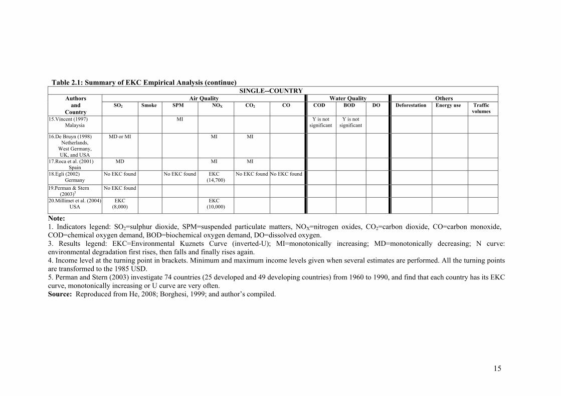
Most of the studies on the EKC addressed the following questions, does an EKC exist
between income and pollution, and if so what is the turning point? The answers from
the results are ambiguous (see Table 2.1), because without a single environmental
indicator, the shape of the income-environment relationship and its turning point
generally depended on the pollutant. Three main categories of environmental
indicators could therefore be distinguished, an air quality indicator, a water quality
indicator, and another environmental indicator.
The evidence of EKC for air quality indicators is strong but not overwhelming
(Galeotti, 2007; Borghesi, 1999). The measures of local air quality (SO2, SPM, CO,
and NOX) generally show an inverted-U shaped curve and an N-shaped curve with
income. This outcome emerged in most of the early studies and seems to be
confirmed by more recent studies although the turning points are different across the

13
indicators where CO and NOX showed higher turning points than SO2 and SPM. Even
when focusing on the same indicator, there are large differences in the turning points
across the studies. The level of global pollutant (CO2) usually increases
monotonically with per capita income (Lantz and Feng, 2006). If there is a turning
point it is at a level beyond the income of most countries. Although some researchers
found evidence supporting the existence of an EKC for CO2, most of them conclude
that the CO2--income per capita relationship was essentially monotonic since most
countries are not expected to reach the turning point, even in the distant future.
The results from the water quality indicators are more mixed than from the air quality
indicators. There was evidence for the EKC relationship for indicators such as COD
and BOD (biochemical oxygen demand) but there were conflicting results about the
shape and peak of the curve. And the N-shaped curve instead of the Inverted U-
shaped curve was mentioned during economic growth where an inverted U-shaped
curve developed but beyond a certain income level the relationship between
environmental pollution and income reverts to being positive.
Many other indicators have been used to test the EKC hypothesis. There was
evidence of an inverted-U curve for deforestation with the peak at a relatively low
income level (Panayotou, 1997), but Shafik (1994) concluded that per capita income
appeared to have little bearing on the rate of deforestation. Moreover, even when an
EKC seemed to exist (energy use and traffic volume), the turning points were far
beyond the observed income range.

14
Table 2.1: Summary of EKC Empirical Analysis CROSS--COUNTRY
Air Quality Water Quality Others Authors SO2 Smoke SPM NOX CO2 CO COD BOD DO Deforestation Energy use Traffic
volumes 1.Grossman & Krueger
(1991) N curve
(Peak:5,000 Trough:14,000)
N curve (Peak:5,000 Trough:10,000)
U curve (9,000)
2.Shafik&Bandyopadhyay (1992)
EKC (3,670)
EKC
MI MI EKC
3.Grossman & Krueger (1995)
N curve (Peak:4,000 Trough:5,000)
EKC (6,151)
MD EKC (7,853)
EKC (7,623)
MI
4.Selden & Song (1994)
EKC (FE:8,916-8,709 RE:10,500)
EKC (9,811)
EKC (12,000)
EKC (6,000)
5.Panayotou (1997) EKC (3,800)
EKC (4,500)
EKC (5,500)
EKC (1,000)
6.Cole et al. (1997) EKC (Log:6,900 Level: 5,700)
EKC (7,300)
EKC (15,100)
EKC (62,700)
EKC (9,900)
MI EKC (34,700)
EKC (65,300)
7.Torras & Boyce (1998) N curve N curve MD MI 8.List & Gallet (2000) N curve
(20,000) N curve (10,000)
9.Barrett & Graddy (2000)
N curve (Peak:4,200 Trough:12,500)
EKC
MI MD MI
10. Bradford et al. (2000)
EKC (3,055)
EKC (11,972)
EKC N curve U curve
11.Stern & Common (2001)
EKC (Whole sample: 29.360 OECD: 48,960 Non-OECD: 303,133)
12.Cole & Elliot (2003) EKC (5,307)
13.Halkos (2003) EKC (2,800-6,200)
14.Kahuthu (2006)
EKC (7,327-9,606)
MI
15
Table 2.1: Summary of EKC Empirical Analysis (continue) SINGLE--COUNTRY
Air Quality Water Quality Others Authors and
Country SO2 Smoke SPM NOX CO2 CO COD BOD DO Deforestation Energy use Traffic
volumes 15.Vincent (1997)
Malaysia MI Y is not
significant Y is not
significant
16.De Bruyn (1998) Netherlands,
West Germany, UK, and USA
MD or MI MI MI
17.Roca et al. (2001) Spain
MD MI MI
18.Egli (2002) Germany
No EKC found No EKC found EKC (14,700)
No EKC found No EKC found
19.Perman & Stern (2003)5
No EKC found
20.Millimet et al. (2004)USA
EKC (8,000)
EKC (10,000)
Note: 1. Indicators legend: SO2=sulphur dioxide, SPM=suspended particulate matters, NOX=nitrogen oxides, CO2=carbon dioxide, CO=carbon monoxide, COD=chemical oxygen demand, BOD=biochemical oxygen demand, DO=dissolved oxygen. 3. Results legend: EKC=Environmental Kuznets Curve (inverted-U); MI=monotonically increasing; MD=monotonically decreasing; N curve: environmental degradation first rises, then falls and finally rises again. 4. Income level at the turning point in brackets. Minimum and maximum income levels given when several estimates are performed. All the turning points are transformed to the 1985 USD. 5. Perman and Stern (2003) investigate 74 countries (25 developed and 49 developing countries) from 1960 to 1990, and find that each country has its EKC curve, monotonically increasing or U curve are very often. Source: Reproduced from He, 2008; Borghesi, 1999; and author’s compiled.

16
2.3.2 Trade and the Environment
The relationship between trade and the environment is one of the main issues where a
clear divergence between pro-environment and pro-trade groups can be found. In the
late 1970s the debate started and it is still hot now. A growing literature on the topic
of trade and the environment suggested that there are a large number of potential
interactions between trade liberalisation and pollution. According to Bhagwati (1993),
Daly (1993) and French (1993), the main arguments between pro-environment and
pro-trade are summarised in Table 2.2. The pro-environment group argues that
increasing trade will maintain pollution-intensive goods in developing countries with
relatively weak environmental regulations and damage their natural resources. The
pro-trade group believes that trade liberalisation enhances economic growth,
promotes the use of a cleaner technology which subsequently improves the
environmental quality.
Table 2.2: Pro-Environment and Pro-Trade Arguments
Until the 1990s a more systematic analysis of the relationship between trade and the
environment has been available, even since Grossman and Krueger (1991) divided
the resultant impact into three independent effects—scale effect, technique effect, and
composition effect.
The growing availability of a large cross-country time-series database combined with
an increasingly powerful computing capacity, has fostered a rapid growth in
quantitative studies of the relationship between trade and the environment. (For an
excellent survey of this literature, see Grossman and Krueger, 1991; Antweiler et al,
2001; Cole and Elliot, 2003; Frankel and Rose, 2002) These studies share the goal of

17
explaining variations in pollution levels by reference to scale, technique, and
composition effects arising from trade liberalisation.
Grossman and Krueger (1991) first used the notion of scale, composition, and
technique effects to assess the environmental impact of the North American Free
Trade Agreement (NAFTA). They used the HO trade model with comparable
measures of three air pollutants in a cross-section of urban areas located in 42
countries to find that concentrations of SO2 and smoke increased with per capita GDP
at low levels of national income, but decreased with GDP growth at higher levels of
income. On the basis of their estimated EKC, Grossman and Krueger concluded that
any income gains created by NAFTA would tend to lower pollution in Mexico. But
there was no relationship between the intensity of pollution and the pattern of U.S.
imports from Mexico because Mexico’s current per capita income placed them on the
declining portion of their estimated inverted-U curve. Because the shape of the EKC
was taken to reflect the relative strength of scale versus technique effect, Mexico was
literally now over the turning point. Relied on both the evidence presented in their
cross-sectional regressions and the results from CGE work by Brown et al. (1992),
Grossman and Krueger found that the composition effect for Mexico was likely to be
slightly beneficial to the environment. Then they combined the evidence on scale,
technique, and composition effects and concluded that trade liberalisation via
NAFTA should be good for the Mexican environment, but if NAFTA led to increased
capital accumulation, then the net impact was less clear. However, they also
concluded that the scale and composition effects of trade on the environment were
negative in Canada and the United States.
Grossman and Krueger’s study was far ahead of existing work in this area because
they used a theoretically based methodology for thinking about the environmental
impacts of trade, and presented empirical evidence on these scores. Future research
was left to improve on their start and deal with some unanswered questions
(Copeland and Taylor, 2004).
Cole and Rayner (2000) followed their methodology in an attempt to measure the
environmental impact of the Uruguay Round trade liberalisation by calculating their
18
implied scale, composition, and technique effects. They found that the emissions of
all five pollutants(SO2, NOX, CO, CO2 and SPM)were predicted to increase in
developing and transition regions as a result of the Uruguay Round, whilst in
developed regions the emissions of three pollutants (SO2, CO and SPM), decreased
and two (NOX and CO2) increased. The environmental impact will be considerably
greater if the Uruguay Round affects the rate of economic growth.
Beghin et al. (1995) analysed the impact of trade liberalisation under better terms of
trade (TOT) with the US, Canada, and Mexico on various pollutants and was able to
find a positive scale effect of liberalisation on pollution, composition and technique
effects were negative, as was the overall impact of trade liberalisation. Hence, they
concluded that trade openness is benefits the environment. In another study Beghin et
al. (2002) analysed the impact of trade reform on Chile’s unilateral liberalisation of
various pollutants without making a distinction between scale, technique, and
composition effects, and concluded that trade liberalisation would increase pollution.
Madrid-Aris (1998) investigated the implications of trade liberalisation under
NAFTA for Mexico, California, and the US. He did not distinguish between the scale
and composition effects or estimate the technique effect. However, he concluded that
there was a positive relationship between trade liberalisation and pollution and that
trade liberalisation had a detrimental effect on the environment.
Antweiler et al. (2001) developed a theoretical model to divide the impact of trade on
pollution into the scale, technique, and composition effects for 43 countries over
1971-1996, and then estimated and collated these effects using SO2 data. They further
estimated a reduced form equation for concentrations of SO2. Among other things
they control for relative factors endowments, the scale of productive activity, the
determinations of policy, and openness to international trade. They found that if
openness to international markets raises both output and income by 1%, pollution
falls by approximately 1%. Therefore they concluded that freer trade was good for the
environment. Copeland and Taylor (2004) also concluded that where trade
liberalisation increases the level of economic activity, the net impact on the
environment was beneficial, although it was only based on SO2 concentrates.

19
Antweiler et al. (2001) gave a different role to theory in developing and examining
the hypotheses and used a consistent data set to estimate all three effects of trade.
They estimated the composition effect jointly with the scale and technique effects on
a dataset that included over 40 developed and developing countries.
Trade liberalisation can have an indirect impact on the environment through the effect
of increasing national income on environmental quality. There are an increasing
number of studies seeking to identify the effect of trade liberalisation on
environmental quality. These studies estimate several pollutants and the results show
that trade liberalisation has multiple simultaneous effects on environmental damage.
Cole and Elliot (2003) used national emissions data to investigate several pollutants.
They were not able to distinguish between scale and technique effects, but used
Antweiler et al.’s (2001) approach to attempt to isolate the composition effect of trade.
They confirmed the Antweiler et al. (2001) results for SO2, and obtained similar
results on composition effects for CO2. However they found that BOD and NOX
appeared to respond differently, suggesting that it was indeed important to expand the
scope of work to include other pollutants. Cole and Elliot concluded that their results
for pollution intensities were more optimistic and trade liberalization would reduce
the pollution intensity of output for all four pollutants. In a model with many
pollutants and goods there was no reason to expect that the relative importance of
pollution haven versus factor endowment motives would be the same across all
pollutants (Copeland and Taylor, 2004).
Frankel and Rose (2002) modelled the effect of trade on the environment, controlling
income and other relevant factors. The main contribution of their paper was to
address the endogeneity of income and especially trade, the latter by means of
instrumental variables drawn from the gravity model of bi-lateral trade. According to
the gravity model trade is determined by indicators of country size (GDP, population,
and land area) and distance between the pair of countries in question (physical
distance as well as dummy variables indicating common borders, linguistic links, and
landlocked status). Such gravity instruments have recently been used to isolate the
effect of trade in studies of economic growth. Using instrumental variables for
20
openness and income, the study focused on seven separate environmental quality
indicators (three measures of air pollution, industrial CO2 emissions, deforestation,
energy depletion and rural clean water access). The results for three types of air
pollution (SO2, NOX and SPM), showed a negative relationship with openness. But
for the other four indicators, only CO2 was found to worsen with trade liberalisation.
The collection of empirical studies mentioned above are summarised in Table 2.3.
Most of these studies only focussed on the scale and composition effects. The scale
effect has consistently been found to increase pollution level but for the composition
effect it was found that trade patterns were strongly influenced by factor intensities.
Few studies estimated the technique effect however, so the results are mixed,
depending on the trade regimes. Chua (1999) stated that the importance of technique
effect has often been ignored because different trade liberalisation regimes have
different effects on input prices and thus lead to different changes in technique.

21
Table 2.3: Summary of Estimations on the Impact of Trade Liberalisation on Pollution Author and country Trade
reform Scale effect
Compositioneffect
Technique effect
Total pollution
1.Grossman & Krueger(1991) Mexico United States Canada
Trade liberalisation with NAFTA
+ + +
- + +
na na na
Small decrease
Increase Increase
2.Beghin et al. (1995) Mexico
Trade liberalisation better terms of tradewith US. and Canada
+2.8%
to +3.7%
-4.3%
to +2.6%
-.7%
to +3.5%
-.2%
to +6.4%
3.Antweiler et al. (2001) Panel of 44 countries
Trade liberalisation +.193%
-1.611%
-
Decrease
Uruguay round reforms
+1.6 to 7.6%
-6.6 to-1.3%
na
-2.5 to 5%
4.Strutt & Anderson (2000) Indonesia
APEC +.3 to +4.1%
-.8.4 to +3.4% na -4.2 to 7.9%
5.Lee &Roland-Holst (1997) Indonesia Japan
Trade liberalisation +.87% +.00%
-.36 to2.86% -.09 to-.02%
na na
+.51 to+3.73%-.09 to -.02%
6.Dessus & Bussolo (1998) Costa Rica
Trade liberalisation +9.4%
+5.6 to+10.6%
+ but small
+15 to+20%
7.Cole & Rayner (2000) EU USA Developing and Transition
Uruguay round trade agreement
No decomposition + + +
+ + -
-.22 to +.37% -.48 to +.33% +.06 to+1.12%
8.Madrid-Aris (1998) Mexico California Rest of United States
Trade liberalisation under NAFTA
No decomposition na na na
+4.683% +0.083% +0.086%
Free trade
No decomposition - -
na na
Decrease Decrease
9.Zhu & van Ierland (2006) EU CEECs EU CEECs
Free trade + mobile labour and capital
+ -
na na
Increase Decrease
Unilateral liberalisation
No decomposition +2.8 to+19.9%
Accession to NAFTA
-4.8 to +3.6%
10.Beghin et al. (2002) Chile
MERCOSUR
-1.2 to +8.1%Combine scale and technique effects
Composition effect
Total pollution
11.Cole & Elliot (2003) Panel of developing and developed countries
Trade liberalisation
SO2: negative BOD: negative NOX,CO2: positive
Positive but small
Uncertain Decrease Increase
Notes: Abbreviation: NAFTA, North American Free Trade Agreement; APEC, Asia-Pacific Economic Cooperation; MERCOSUR, Common Market of the Southern Cone; EU, European Union; CEECs, Central and Eastern European Countries. Source: 1, 2, 4, 5, 8, and 10 are reproduced from Chua, 1999.

22
2.3.3 Computable General Equilibrium (CGE) models
With the advance in modelling tools and increasing worldwide concerns for the
sustainability of greater trade liberalisation and higher income growth, there have
been many studies investigating different aspects of the complex trade- environment
nexus, most of which deployed Computable General Equilibrium (CGE) techniques.
CGE models are multi-sector numerical models based on concepts usually associated
with Walrasian general equilibrium theory. Now CGE models have been fruitfully
used for quantitative analysis of environmental and natural resource problems and
related policy issues in a national, multi-national or global economy.
Zhu and van Ierland (2006) used a comparative static CGE model to assess the effects
of EU enlargement in terms of increased regional trade on greenhouse gas emissions.
Freer trade between union members was argued to have positive economic welfare
impacts and not necessarily lead to an increase in greenhouse gas emissions. O’Ryan
et al. (2005) used a static CGE model for the Chilean economy to highlight the
importance of coordinating environmental and trade policies. The authors argued that
the negative consumption, output, and impact on trade of an environmental tax
reform (increase in fuel taxes) may be mitigated to some extent through a
corresponding reduction in tariffs. However, the net outcome in terms of achieving
better average results depends on sectors energy patterns and relationship to external
trade. Beghin et al. (2002) looked at the health and environmental impact of three
different trade integration scenarios: access to the North American Free Trade
Agreement (NAFTA), Common Market of the Southern Cone (MERCOSUR) and
uni-lateral liberalisation. Joining NAFTA was argued to be environmentally benign
due to trade diversion contributing to lower use of cheap energy, whereas access to
MERCOSUR and a uni-lateral opening to world markets would increase
environmental damage and raise urban morbidity and mortality rates as access to
cheaper and dirty energy inputs was enhanced.
The limitations of CGE models are as following. First, CGE models are typically
constructed to target aggregates, but not to deal with complex environmental impact
related to its affect on biodiversity and stocks of natural resources. Second, CGE
models require many assumptions and large amount of parameters, and then focus on
23
forecasting issues. However, with many sectors it is hard to make realistic forecast
estimations in a dynamic framework. In addition, CGE models only partly address
trade liberalisation-induced climate change in terms of energy-linked emissions (e.g.
CO2 greenhouse gas emissions), therefore the assessment of the impact of trade
liberalisation on the major environmental quality indicators was poorly estimated
under the CGE approach.
2.4 Conclusion
The HO theory is consistent with the argument that increased specialisation increases
the volume of pollution-intensive goods, and then more emissions. However, the
Stolper-Samulson Theorem predicts that if externalities are internalised, firms would
shift to less pollution-intensive production. Grossman and Krueger (1991) used those
theories to decompose the impact of trade liberalisation on environment into scale,
technique, and composition effects. The EKC curve captures some of those effects.
The theoretical framework of the trade-growth-environment nexus was validated by
the empirical studies on trade related emissions. It was in the measurement problem
that empirical studies differed from each other. Inconsistency in time, country, and
methodology put a barrier between any meaningful comparisons of the studies. Most
of the empirical studies surveyed here, in general, found mixed results for (a) the
EKC hypothesis, the air quality indicators were stronger evidence than other
indicators; (b) trade related emissions in the light of scale, technique, and
composition effects as theory predicted; and (c) CGE models which provided a
quantitative assessment of competing models to sort out various hypotheses. The
turning point income varied depending on countries and time. It was predicted that
countries which are currently in the process of development are more likely to learn
from the mistakes of developed countries and therefore reach the turning point
income relatively soon. If we examine the experience of an individual country at
various levels of development this may be true because as Vincent (1997) pointed out,
the cross-country version of the EKC is misleading. The source of income and
expenditure pattern varies across countries. Cross-country regression related policy
variables seem to be sensitive to slight alterations in the policy variables and to small
24
changes in the samples of countries chosen. The CGE model was used to predict but
may not be able to analyse past performances.
The next chapter will present a discussion of Chinese economy, including economic
reforms started in 1978, economic growth and international trade performances.

25
CHAPTER THREE
THE ECONOMY OF CHINA 3.1 General Background
The People’s Republic of China (PRC), commonly known as China, is the largest
country in East Asia and the most populous in the world with over 1.3 billion people
in 2007, and with a growth rate of approximately 0.6 per cent has approximately a
fifth of the world’s population. It is a socialist republic ruled by the Communist Party
of China under a single-party system and has jurisdiction over twenty-two provinces,
five autonomous regions, four municipalities, and two Special Administrative
Regions. The capital of the PRC is Beijing.
At 9.6 million square kilometres, the PRC is the third largest country in the world
after Russia and Canada. Han and other 55 other minorities have been living in China
for over 5000 years. There are seven major Chinese dialects (Mandarin, Wu, Yue,
Min, Xiang, Hakka and Gan) and many sub-dialects. Mandarin is the official
language and is spoken by over 70% of the population. The remainder, concentrated
in the southwest and southeast, speak one of the six other dialects. Non-Chinese
languages spoken widely by ethnic minorities include Mongolian, Tibetan, Uygur and
other Turkic languages (in Xinjiang), and Korean (in the northeast).
The PRC holds a permanent seat on the UN Security Council and membership in the
WTO, APEC, East Asia Summit, and Shanghai Cooperation Organisation. China is
one of the world’s fastest growing economies. It has the world’s fourth largest GDP
in nominal terms and consumes as much as a third of the world’s steel and over half
of its concrete. The PRC is also the world’s second largest exporter and the third
largest importer in 2007. Since the economic reforms in 1978, the poverty rate in the
PRC has decreased from 64% in 1981 to 10% in 2004.
To capture the economic and environmental performance of China, this chapter is
organized as follows: China’s reform is presented in section 3.2, including the pre-
reform (before 1978) and post-reform (since 1978), detailing the reforms in different

26
regions; China’s growth, and international trade performances are introduced in
section 3.3; finally, this chapter is summarised in section 3.4.
3.2 China’s Reforms
This section identifies pre-reform (before 1978) and post-reform (since 1978).
3.2.1 Pre-reform: 1949-1978
After 1949 China followed a socialist heavy industry development strategy, or the
“Big Push industrialization” 6 strategy. To implement this strategy, a planned
economic system, often called “command economy”7, was phased in during this
period.
Consumption was reduced as rapid industrialisation was given high priority. The
government took control of a large part of the economy and redirected resources into
building new factories. Investment, all of which was government investment,
increased rapidly to over a quarter of the national income. By 1954 China had pushed
its investment rate up to 26% of GDP. Investment rose further during the Great Leap
Forward (GLF, 1958-1960), but then crashed after the GLF. Over the long term
China’s investment rates have been high and rising.
Most investment went into industry and more than 80% of industrial investment was
in heavy industry. With planners pouring resources into industry, rapid industrial
growth was not surprising. Between 1952 and 1978, industrial output grew at an
average annual rate of 11.5%. Moreover, industry’s share of total GDP climbed
steadily over the same period from 18% to 44%, while agriculture’s share declined
from 51% to 28%. At the same time China’s economy began to grow dramatically.
Throughout the 1950s and 1970s a number of widespread changes occurred in
China’s economic policies and procedures. During the First Five-Year Plan (FYP)
(1953-1957), a policy of continued rapid industrial development was continued
6 “Big Push” means Chinese government gave overwhelming priority to channelling the maximum feasible investment into heavy industry. 7 “Command economy” means market forces were severely curtailed and government allocated resources directly through their own command.

27
because the first policies plan, rapid growth in heavy industry, was achieved. A few
months after the introduction of the Second FYP (1958-1962), which was to be
similar to the First one, the policy of the Great Leap Forward was announced. In
agriculture it involved the formation of people’s communes, the abolition of private
plots, and an increasing of output through greater cooperation and physical effort.
Construction of large factories was to be continued apace. However the peasantry
were not prepared for this communal system. Concurrently, the irregular and
haphazard backyard production drive failed to achieve the intended objectives as it
turned out enormous quantities of expensively produced, low quality goods, most
notably steel produced from low quality iron which cannot be used for building (Chan,
2001).
3.2.2 Post-reform: 1979-present
China’s economic reforms have been placed in the all regions, including agriculture,
enterprise, trade and investment, since December 1978 “Third Plenum of the 11th
Central Committee”.
3.2.2.1 Rural Economic Reform
The Third Plenum in December 1978 made relatively modest adjustments to rural
policy. Two major policies were adopted at the beginning of agricultural reforms,
price increases for agricultural products in 1979 and a reaffirmation of the right to
self-management of collectives in 1981 (Nicholas, 1983). A household responsibility
system, a nationally defined program of contracting land to households, emerged in
1981. Farmers were able to retain surplus over individual plots of land rather than
farming for the collective. Private ownership of production assets became legal. By
the end of 1982 more than 90% of China’s agricultural households had returned to
some form of household farming. Initially land was contracted to households for one
year, and then it was succeeded by 5, 15, 50- year because it was seen that contracts
should be longer to be more effective.
The growth of grain production accelerated dramatically. Between 1983-1985 grain
output growth jumped to 4.1% annually from a previous 2.2%. During the 1990s
output growth was actually greater in every sector of agriculture. Cotton and oilseed

28
production grew at 15% and 16% per year, respectively. Meat production surged,
growing at just below 10% per year. China’s entry into the WTO is having an
important impact on agricultural development. A new round of subsidies and tax
reductions that began in 2004 promised to put the national government in the position
of providing net support for agriculture for the first time since 1949.
Rural industry, known as township and village enterprises (TVEs), has been an
important part of China’s rural economy. Since 1978 the government encouraged
non-agricultural activities in rural areas. Between 1978 and the mid-1990s, TVEs as
publicly owned enterprises experienced a golden age of development. TVEs played
an important role in rural reform, such as increasing incomes, absorbing rural labour
released from farms, and then narrowing the urban-rural gap. TVEs employment
grew from 28 million in 1978 to a peak of 135 million in 1996, with a 9% annual
growth rate. The share of GDP increased from less than 6% in 1980 to 26% in 1996.
After 1996 TVEs underwent a further dramatic transformation: privatisation. Table
3.1 makes it clear that private ownership is now the dominant form of TVEs.
Table 3.1: TVE Employment by Ownership, 2003
3.2.2.2 Enterprise Reform: SOEs and Non-SOEs
Development of SOEs
Enterprise reform is the central problem in this entire transition process. State-owned
industrial enterprises (SOEs) were the core of the old command economy. Since the
1950s traditional SOEs dominated, but in 1978, SOEs produced 77% of industrial
output. Collective enterprises were factories that were nominally owned by the

29
workers in the enterprise but were actually controlled by local government. They
produced 23% of output. The dominant SOEs were responsible for the welfare, health,
and political indoctrination of their workers.
Based on the poor performance, low profitability, and inferior competitiveness of
SOEs, enterprise reform measures with the main theme of “expanding enterprise
autonomy and profit retention to enterprises” was extended nationwide in 1979.
These reform measures gradually disengaged SOEs from a traditional planned
economy and let them begin to participate in and adapt to market competition with
non-state enterprises (Wu, 2005). Then a few high performance SOEs emerged.
The adoption of the Company Law in 1994 was a milestone of industrial reform. This
Company Law stipulated that traditional SOEs must convert into the legal form of a
corporation and provide a pertinent framework. Tens of thousands of SOEs and
collective firms were shut down. 40% of the SOEs workforce were laid off and more
than two-thirds of the collective workforce.
By 1996 over half of China’s SOEs were inefficient and reporting losses. During the
15th National Communist Party Congress met in September 1997, President Jiang
Zemin announced plans to sell, merge, or close the vast majority of SOEs. Then a
new policy called “grasping the large, and letting the small go” was adopted. The
largest, typically centrally controlled firms, were restructured and financed but kept
them under state control, while firms owned by local governments were privatised or
closed down. In 2000, China claimed success in its three-year effort to make the
majority of large SOEs profitable.
Development of Non-SOEs
In 1956, as private enterprises were eradicated in China, the Chinese economy
became dominated by state ownership. However, the market economy was
considered impossible to set up based on a monopoly of state ownership. Reform was
aimed at integrating China more fully into the international economy (Wang, 1984).
Individual business sector first emerged in the rural area. During the 1980s and early
1990s contracted family farms and TVEs developed rapidly and had become an
30
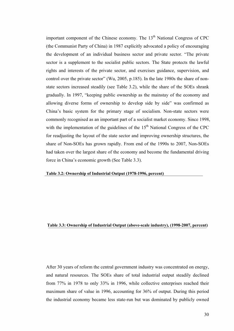
important component of the Chinese economy. The 13th National Congress of CPC
(the Communist Party of China) in 1987 explicitly advocated a policy of encouraging
the development of an individual business sector and private sector. “The private
sector is a supplement to the socialist public sectors. The State protects the lawful
rights and interests of the private sector, and exercises guidance, supervision, and
control over the private sector” (Wu, 2005, p.185). In the late 1980s the share of non-
state sectors increased steadily (see Table 3.2), while the share of the SOEs shrank
gradually. In 1997, “keeping public ownership as the mainstay of the economy and
allowing diverse forms of ownership to develop side by side” was confirmed as
China’s basic system for the primary stage of socialism. Non-state sectors were
commonly recognised as an important part of a socialist market economy. Since 1998,
with the implementation of the guidelines of the 15th National Congress of the CPC
for readjusting the layout of the state sector and improving ownership structures, the
share of Non-SOEs has grown rapidly. From end of the 1990s to 2007, Non-SOEs
had taken over the largest share of the economy and become the fundamental driving
force in China’s economic growth (See Table 3.3).
Table 3.2: Ownership of Industrial Output (1978-1996, percent)
Table 3.3: Ownership of Industrial Output (above-scale industry), (1998-2007, percent)
After 30 years of reform the central government industry was concentrated on energy,
and natural resources. The SOEs share of total industrial output steadily declined
from 77% in 1978 to only 33% in 1996, while collective enterprises reached their
maximum share of value in 1996, accounting for 36% of output. During this period
the industrial economy became less state-run but was dominated by publicly owned

31
firms. Since 1998 the National Statistics Bureau has only reported data on the output
of the above-scale firm8. As Table 3.3 shows, the SOEs share of this above-scale
industrial sector continued to gradually decline, while the share of collective firms
dropped dramatically. After reaching a peak of importance in 1996, collective firms
are now rapidly privatising. Foreign invested firms and private enterprises continue to
gain in importance, but at a moderate pace.
3.2.2.3 Trade Reform
Since 1978 China has undergone a significant transition from a plan-oriented foreign
trade system to a market-oriented foreign trade system by conducting a series of
reforms in their foreign trade system.
China’s first opening step came in 1978 when Hong Kong businesses were allowed to
sign Export-Processing (EP) contracts with Chinese firms in the Pearl River Delta. In
this way an export production network already created by Hong Kong could expand
into China. Shortly after this, four special economic zones (SEZs) were set up in the
southern provinces of Guangdong and Fujian. These SEZs allowed imports in duty-
free, as long as they were used in the zone to produce exports (Park, 1997). By the
mid-1980s China began the task of liberalising the main national trading system. The
main elements9 of this reform include the following:
1. Devaluation. Before reform China maintained an overvalued currency. In 1980
there were 1.5 Chinese yuan to the US dollar. By 1986 the value of the Chinese
currency had declined to 3.5 to the dollar. In 1986 a dual-exchange-rate regime was
introduced in which exporters outside the plan could sell their foreign-exchange
earnings on a lightly regulated secondary market.
2. De-monopolisation of the foreign-trade regime. A number of foreign trade
companies were allowed to be set up, the provincial branches of former national
8 Above-scale firm are state-owned firms and non-state firms with an annual output value of more than 5 million RMB (US$600,000). 9 Naughton, 2006, pp.380-386.

32
foreign trade monopolies became independent; and many local governments and
SEZs set up trading companies.
3. Significant change in pricing principles. Profit retention and bonuses provided
incentives, decentralisation increased competition, and devaluation made exporting a
potentially lucrative business.
4. Creation of a system of tariff and non-tariff barriers.
5. Import substitution and export promotion. By the mid-1980s China had moved
from a planned trading system to one of high tariffs, multiple non-tariff barriers, and
abundant administrative discretion.
At the same time, in order to simplify the exporting process and reduce the
centralised foreign trade monopoly, an export processing trade regime has been
created. It enabled China to adopt relatively liberal rules on export processing trade
while still protecting the domestic market. These rules enabled China to
accommodate the wishes of foreign investors and helped bring China into
increasingly integrated cross-border production networks. These 1980s reforms
created the dramatic export success that came later.
From the mid-1990s a new era of a genuinely open economy began in China.
Membership in the WTO was a powerful motivating factor. During the fifteen years
of negotiation after applying to join the WTO, China instituted reforms in many areas
related to trade. For example, tariff barriers were significantly lowered from 43% in
1992 to 17% in 1999, most import quotas were abolished and the laws were improved.
In 1994 China abolished the secondary swap market for foreign exchange. The
official exchange rate was merged with the market rate under a managed floating
exchange rate system and the convertibility of the currency under the current account
was achieved within three years. At the same time the national taxation system was
shifted to a much higher reliance on value-added taxes (VAT). After the taxation
reforms of 1994 China promoted exports by tax rebates and began to offer VAT
rebates on exports.

33
On 11th December 2001 China finally became the 143rd member of the WTO. It
meant that China accepted the rules of globalisation to some extent. On the trade side,
the most fundamental issue was the requirement that China opened up the ordinary-
trade regime and dramatically reduce the dual trade regime. Eventually, a new
provision, that China’s commitment to extend trading rights without restrictions,
including domestic and foreign private companies, was introduced in a foreign –trade
law in 2004 (Wu, 2005). Under this law the Chinese government no longer restricts
trade to a limited number of state-owned foreign trade companies. The average
nominal tariff was reduced from 15% in 2002 to 9.4% in 2007.
3.2.2.4 Foreign Direct Investment Reform
China decided to accept foreign investment in 1978 and in 1979 and 1980 established
Special Economic Zones (SEZs). Foreign direct investment (FDI) grew steadily
through the 1980s and made important changes to the regional economies of
Guangdong and Fujian. Nationwide the impact of FDI began early in the 1990s,
especially the remarkable speeches Deng Xiaoping made during a famous “Southern
Tour” in the spring of 1992. China began to selectively open the domestic
marketplace to foreign investors. More foreign investors participated in new sectors,
especially real estate; and more rights were granted to foreign manufacturers to sell
their products on the Chinese market.
The proliferation of special investment zones of various kinds was the main reason
for attracting foreign investors. By 2003 there were over 100 investment zones
recognised by the central government. There are six SEZs (Shenzhen, Zhuhai,
Shantou, Xianmen, Hainan, and Pudong), 54 national-level ETDZs (Economic and
Technological Development Zones), 53 nationally recognised high-tech industrial
zones, and 15 Bonded Zones (in which commodities can be legally parked outside the
country’s customs borders). There are hundreds of zones run by local government
without central support. Taxes are moderate, investment protection agreements and
an apparatus for arbitration are available, most legal provisions are adequate in
principle, the currency is convertible in the current account, there are relatively
decentralised natures, a high degree of discretion is retained by government officials,
and approvals can be granted by local investment boards.

34
FDI grew steadily through the 1980s and made important changes in the regional
economics of Guangdong and Fujian. Investment began to pour into China after 1992,
and annual inflows have been over 40 billion dollars since 1996. Trending steadily
upward, FDI inflows was $75 billion dollars in 200710 (Figure 3.1). For more than a
decade the cumulative level of FDI in China at the end of 2007 stood at nearly $760
billion, making it one of the world’s largest destinations for FDI. China has accounted
for about one-third of total developing-country FDI inflows in recent years.
Figure 3.1: Annual Utilised Foreign Direct Investment, 1985-2007 ($ billions)
Based on cumulative FDI for 1979-2007, about 40% of FDI in China has come from
Hong Kong, 9.7% from the British Virgin Islands, 8.1% from Japan, and 7.4% from
the USA (See Table3.4).
Table 3.4: Major Foreign Investors in China: 1979-2007 ($ billions and % of total)
10 FDI data excluded investment in the banking, insurance, and securities sectors. FDI including financial sector totalled $82.7 billion in 2007.
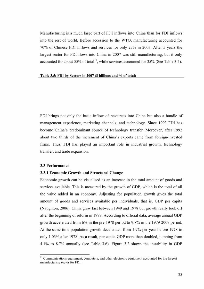
35
Manufacturing is a much large part of FDI inflows into China than for FDI inflows
into the rest of world. Before accession to the WTO, manufacturing accounted for
70% of Chinese FDI inflows and services for only 27% in 2003. After 5 years the
largest sector for FDI flows into China in 2007 was still manufacturing, but it only
accounted for about 55% of total11, while services accounted for 35% (See Table 3.5).
Table 3.5: FDI by Sectors in 2007 ($ billions and % of total)
FDI brings not only the basic inflow of resources into China but also a bundle of
management experience, marketing channels, and technology. Since 1993 FDI has
become China’s predominant source of technology transfer. Moreover, after 1992
about two thirds of the increment of China’s exports came from foreign-invested
firms. Thus, FDI has played an important role in industrial growth, technology
transfer, and trade expansion.
3.3 Performance
3.3.1 Economic Growth and Structural Change
Economic growth can be visualised as an increase in the total amount of goods and
services available. This is measured by the growth of GDP, which is the total of all
the value added in an economy. Adjusting for population growth gives the total
amount of goods and services available per individuals, that is, GDP per capita
(Naughton, 2006). China grew fast between 1949 and 1978 but growth really took off
after the beginning of reform in 1978. According to official data, average annual GDP
growth accelerated from 6% in the pre-1978 period to 9.8% in the 1979-2007 period.
At the same time population growth decelerated from 1.9% per year before 1978 to
only 1.03% after 1978. As a result, per capita GDP more than doubled, jumping from
4.1% to 8.7% annually (see Table 3.6). Figure 3.2 shows the instability in GDP
11 Communications equipment, computers, and other electronic equipment accounted for the largest manufacturing sector for FDI.
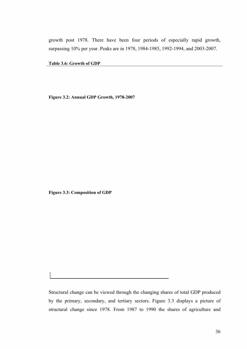
36
growth post 1978. There have been four periods of especially rapid growth,
surpassing 10% per year. Peaks are in 1978, 1984-1985, 1992-1994, and 2003-2007.
Table 3.6: Growth of GDP
Figure 3.2: Annual GDP Growth, 1978-2007
Figure 3.3: Composition of GDP
Structural change can be viewed through the changing shares of total GDP produced
by the primary, secondary, and tertiary sectors. Figure 3.3 displays a picture of
structural change since 1978. From 1987 to 1990 the shares of agriculture and
37
industry declined slowly, while the service sector grew rapidly. Since 1991 the share
of industry has increased and levelled off between 45% and 50% of GDP.
Agriculture’s share of GDP during this period declined rapidly, sliding from 27% of
GDP in 1990 to 11% in 2007, and service’s share of GDP increased from 31% in
1990 to 40% in 2007. China has successfully rapidly transferred from a
predominantly agricultural economy to an industrialised economy.
3.3.2 The Development of Foreign Trade
China began trade liberalisation with one of the most closed economies in the world.
During the thirty years from 1978 to 2007, the volume of China’s foreign trade
increased dramatically, especially after 2002. The total amount of imports and exports
in 2002 increased by twenty-five times and increased in 2007 by more than one
hundred times (see Figure 3.4). China’s rank in world trade jumped from No. 32 in
the early stage of the opening up to No. 3 in 2005, after US and Germany. China’s
export has grown dramatically in recent years, doubling in size from 2004 to 2007,
with an average annual growth rate of 29%, while imports increased by 70%. China’s
trade surplus surged in 2007to $262 billion from $32 billion in 2004.
With the continuous growth of foreign trade, China’s trade dependence ratio12 also
increased. The trade dependence ratio before 1978 never exceeded 10% and reached a
low point of only 5% in 1978. Over the past 30 years China’s position has changed
dramatically. Figure 3.5 shows China’s trade dependence ratio. In 1978 the trade ratio
was far below world average. Between 1980 and the early 1990s, China rapidly
opened up and converged quickly to world average. The trade share stabilised
through the late 1990s. Since 2002, trade has surge again, and then China was
acknowledged as a global trade power. In 2007 China’s total goods trade (exports
plus imports) amounted to 85% of GDP, far more than other large economies such as
the US, Japan, India, and Brazil, which have trade/ GDP ratios of around 20%. At the
same time the composition of trade has shifted from primary products to
manufactures, which were half the exports (two-thirds of imports) in 1980 but nine-
12 The trade dependence ratio is the index used to measure the degree of opening up and dependence of an economy on the international commodity market, usually by the ratio of total volume of imports and exports to GDP, ratio of exports to GDP, or ratio of imports to GDP.

38
tenths of exports ( four-fifths of imports) in 2000 and 94% of exports (76% of imports)
in 2006 (Table 3.7). Trade liberalisation has been an important part of China’s
economic reform process since its conception.
Figure 3.4: Growth of China’s Foreign Trade ($ 100 million)
Figure 3.5: Trade Dependence Ratio (% of GDP)
Table 3.7: Composition of China’s Exports and Imports (% of total)

39
According to the statistical data China’s major trading partners in 2007 were the
European Union (EU), the USA, the Association of Southeast Asian Nations 13
(ASEAN), and Hong Kong (See Table 3.8). China’s largest export markets were the
EU, USA, and Hong Kong, while imported from Japan, EU, and ASEAN.
Table 3.8: China’s Major Trading Partners, 2007 ($ billions)
Trade surpluses, large-scale foreign investment, and large purchases of foreign
currencies to maintain its exchange rate with the dollar and other currencies have
enabled China to accumulate the world’s largest foreign exchange reserves (Morrison,
2008). This accumulation has risen rapidly over the past few years (see Figure 3.6) to
$1.5 trillion at the end of 2007.
Figure 3.6: Foreign Exchange Reserves ($ 100 billions)
3.4 Conclusion
After three decades of economic reform, beginning in 1978, China has transformed
itself from a centrally planned economy to a market economy. The pre-1978 policies
13 ASEAN members are Indonesia, Malaysia, Philippines, Singapore, Thailand, Brunei, Cambodia, Laos, Myanmar, and Vietnam.

40
were more inward-oriented by enforcing import-substitution strategies and
incorporating more government control on all activities. The reform in 1978 focused
more on gradualist, dual-track, decentralising, and from 1993 to the present, more on
macro-economic capacity.
From 1979 to 2007 China’s GDP grew at an average annual rate of 9.8%. Real GDP
grew 11.4% in 2007. China is expected to continue to enjoy rapid economic growth
in the years ahead. International trade and foreign investment continue to play a major
role in China’s booming economy. From 2004 to 2007 the total value of trade of
Chinese merchandise nearly doubled. In 2007 China’s exports exceeded US exports
for the first time. However, studies reveal a consistent conclusion that reform is an
“unfinished agenda” and they note inadequacies in reform. Macro-economic policy is
lacking in efficiency while human capital development is running behind. The
pressures of rapid economic development are gradually eroding the deflationary
effects in the Chinese economy. Therefore, the important challenges are to accelerate
reforms to the financial sector, strengthen monetary policy, and diversify economic
expansion away from the present explicit emphasis on exports and gradually
liberalise the foreign exchange market.
The reforms in 1978 and 1992 raised two questions, one with regard to the success in
her attempts to reform, and the other is the impact on the environment. The growing
fear with the second question is that China might end up as a big polluter in the world.
Chapter four will address this issue.

41
CHAPTER FOUR
ECONOMIC GROWTH AND THE ENVIRONMENT IN CHINA
4.1 Introduction
The market-oriented economic reforms that started in 1978 have greatly transformed
the Chinese economy. Recent official data shows that during the period of the 10th
Five-Year Plan (FYP) (2000-2005), China’s economic development indicators
surpassed the goals and GDP registered a 9.84% annual average growth. At the end
of 2007 it reached 10.8%. In contrast, China’s reduction in emissions or discharges
fell short of the targets for a number of pollutants in absolute terms. In 2005 the SO2
emissions increased by 27% from its 2000 level, exceeding the target by 7.5 million
tons and the COD emissions reached 14.13 million tons, 8% higher than the target.
The target of decreasing emissions by 10% for SO2 and COD are stipulated in the 11th
FYP (2006-2010) 14 . In 2007, for the first time, both SO2 and COD emissions
decreased by 3.2% and 2.3% from 2005 level, respectively.
Given China’s rapid pace of growth, its performance in environmental protection
inevitably attracted attention. Researchers began to ask the following questions. Will
the environmental conditions improve automatically at higher income levels? If so,
what is the turning point income in China? Given the significant regional differences
in industrial structures, levels of urbanisation and stages of development, does the
relationship between economic growth and the level of pollutant emissions differ
across regions? And what should the government do about environmental degradation?
This chapter aims to test the availability of the Environmental Kuznets Curve (EKC)
in China based on provincial data from 1990 to 2007. This chapter intends to analyse
the relationship between GDP per capita and the emissions of four industrial
pollutants (SO2, smoke, dust, and COD). In addition it will study the impact of the
geographic location to see whether there are any differences when all provinces have
been considered as a whole, or grouped into three regions, coastal, central, and
western.
14 The National 11th Five Year Plan for Environmental Protection (2006-2010).

42
The rest of this chapter is organised as follows: section 4.2 describes the phases of
China’s economic development and environmental problems; section 4.3 presents the
legislation on environmental standards; the literature review about China is presented
in section 4.4; section 4.5 provides the model specifications and a description of the
data; Section 4.6 reports the empirical results; finally, section 4.7 concludes and
discusses policy implications.
4.2 China’s Economic Development Phases and Environmental Problems
China’s environmental problems are closely related to progress in industrialisation.
There are five phases of economic growth during this period15:
(1) Socialist heavy-industry-priority development—1949 to 1978;
(2) Rural reform—1979 to 1984;
(3) Light industry development—1985 to 1992;
(4) Preliminary heavy chemical industry development—1993 to 1999;
(5) Heavy chemical industry development—2000 to now.
The economic growth in each phase has distinct characteristics which brought about
different environmental problems.
4.2.1 Early Stage (1949-1978)
From 1949 to 1978, China experienced the “Great Leap Forward” and “Cultural
Revolution” which had caused fairly severe environmental pollution and ecological
damage. However due to the small scale production and large environmental capacity
the contradiction between economic construction and environmental protection was
not prominent, and environmental problems remained in controllable regional scope
(Xia et al., 2007).
After 1978 the whole country began to strenuously develop the economy, all work
was carried out around economic construction and various development projects
commenced and economic growth accelerated sharply. With this high speed
economic growth the volume of pollutants discharge increased rapidly and the
15 See Wang, 2005 and CAS, 2006.

43
conflict between environmental protection and economic development became
increasingly prominent.
4.2.2 Initial Emergence of Environmental Problems (1978-1984)
During this period China experienced economic reform and opened up by initiating
rural reform and agricultural development. In 1984 both industrial and agricultural
production value doubled over 1978, especially in the industrial sector where
township enterprises grew rapidly. Though this phase featured rural land reform, the
non-point source of agricultural pollution was not severe due to backward agricultural
processes and a limited supply of production materials such as pesticides and
fertilisers (Xia et al., 2007). Due to the large number of randomly scattered township
enterprises with irrational production structures, poor technical equipment and
management, and a large consumption of resources and energy and lack of
preventative measures pollution became even more prominent and harder to prevent.
Pollution had spread from hot spots to the whole region, extending from urban to
rural areas. During this period environmental protection work lagged far behind
economic development.
4.2.3 Emergence of Environmental Problems (1985-1992)
China’s economic development during this period was primarily the rapid
development of light industry, mainly light and textile industries to meet the demand
for food, clothing, and other consumptions. By 1988 the symptoms of economic
overheating had become quite evident with some areas and departments blindly
adopting projects with high energy consumption, low efficiency, waste of resources
and heavy pollution, such as small scale paper mills, electroplating, coking and
smelting plants. Moreover, deforestation and overexploitation of natural resources
was common, which accelerated the deterioration of the environment. Urban air
pollution was particularly severe. The average annual value of suspended particulates
exceeded 800mcg/m3 in the northern urban area and exceeded 1,000mcg/m3 in some
cities in winter. Water quality suffered even worse. The MEP reported that 436 of
532 rivers had been polluted at different levels, and among the 15 major urban
reaches of the seven largest rivers, 13 were severely polluted. In addition, the
aggregate untreated industrial residues and urban domestic waste amounted to 6.6

44
billion tons and occupied a 536km2 area of land and had become the second largest
source of pollution. The coverage of land with soil and water loss increased from
1.16mn km2 to almost 1.50mn km2 (Qu, 1989).
4.2.4 Increasingly Serious Environmental Problems (1993-1999)
During this period China experienced accelerated industrialisation and urbanisation,
especially in the 9th Five-Year Plan (1996-2000) where the actual average annual
growth of GDP reached 8.3%. The proportion of heavy industry significantly
exceeded light industry and high growth industries included energy and raw materials
such as oil and natural gas, infrastructure and basic industries such as highways, ports
and electricity, electrical products such as colour TV, refrigerators, washing machines
and air conditioners, etc... In 1999 China’s urbanisation rate was 30.9%, 1.7 times
that in 1978 (Ren and Chen, 2006).
During this period the main challenges were continuous geographic expansion of
ecological deterioration caused by high energy consuming economic growth and
backward technological and management levels which lead to slower treatment than
pollution and destruction. Within seven years the industrial wastewater discharged
was 144.9 billion tons, industrial gas emissions averaged 77 trillion m3, and the total
industrial SO2 emissions amounted to 98.18 million tons. As a result, environmental
pollution and ecological damage had not only impeded the economy in certain
regions, but affected people’s health (Li, 1996).
4.2.5 Intensive Outburst of Environmental Problems (2000 to now)
China entered an era of heavy chemical industry during this phase. Industries such as
electricity, steel, mechanical equipment, cars, shipbuilding, chemicals, electronics,
and building materials became the main drives of economic growth to meet the
demand for high consumption of housing and travelling. After 2003 China
experienced even more rapid economic growth at a rate exceeding 10% in 5
consecutive years, and according to the World Bank, China’s GDP (nominal) per
capita exceeded US$2,485 in 2007, following the level of US$1,100 in 2002. This
phase witnessed the fastest and most long lasting economic growth and experienced

45
accelerating urbanisation. In 2007 the rate of urbanisation reached 44.9% and an
average annual increase of 1.3%.
At the same time the consumption of resources and energy increased significantly.
Coal consumption rose from 1.376 billion tons in 2000 to 2.58 billion tons in 2007,
an increase of almost 87.5%, which directly resulted in high emission of main
pollutants. In particular, emissions of SO2 and COD in 2007 were 24.681 million tons
and 13.818 million tons respectively.
China’s air pollution is recognised as one of the worst in the world. According to the
Blacksmith Institute16 -- (an independent environment group), two of the top ten
worst polluted places are in China17. Figure 4.1 shows that about 60% of cities above
county level are likely to meet the grade II ambient air quality standard by 2007. The
SO2 concentration in urban air, after dropping steadily since the early 1990s, began to
increase again in 2002. Nationwide SO2 emissions, after increasing by 13% during
2000- 2006, finally decreased about 3.2% in 2007 in comparison to last year.
Meanwhile, more than a quarter of China’s seven major rivers are still highly polluted
(grade V or above) in 2007, but the seven major rivers showed a strong improvement
over 2001-2007 (see Figure 4.2). The percentage of monitored sections of the seven
major rivers that met a grade III quality standard or better rose from 30% to 50%.
However, more than half of China’s major lakes and reservoirs were still highly
polluted (grade V or above) in 2007 (see Table 4.1). The water quality of three major
national lakes (Dianchi in Kunming, Chao in Anhui, and Tai in Jiangsu) has not
significantly improved over the last few years, while those lakes are still in grade V.
16 The Blacksmith Institute (2007), founded in 1999, is a New York City based organization supporting pollution-related environmental projects. 17 The Blacksmith Institute (2007) announced top ten worst polluted places. They are Sumgayit, Azerbaijan; Linfen, China; Tianying, China; Sukinda, India; Vapi, India; La Oroya, Peru; Dzerzhinsk, Russia; Norilsk, Russia; Chernobyl, Ukraine; Kabwe, Zambia.

46
Figure 4.1: Urban Air Quality

47
Figure 4.2: Water Quality Comparison of the Seven Major Rivers
Table 4.1: Water Quality of Major Lakes and Reservoirs, 2007
4.3 Legislation on Environmental Standards
In order to protect public health and environmental quality the government has
undertaken a series of actions. Several laws, regulations, and standards have been
promulgated (Edmonds, 2004).
The decision making system of environmental policy in China consists of three
organisations. First, the National People’s Congress (NPC) has a committee called the
Environmental and Resources Protection Committee (ERPC) which is responsible for
48
environmental policy. The NPC makes policy decisions for environmental protection,
passes legislation, and supervises its enforcement. Second, the State Environmental
Protection Commission (SEPC) of the State Council drafts policies, regulations, and
laws for environmental protection. Third, the Ministry of Environmental Protection
(MEP) for the State Council administers and supervises environmental protection
laws throughout the country18. Five regional inspection offices were established in
2006 in an effort to foster regional coordination. The local Environmental Protection
Bureaus (EPBs) and Environmental Protection Offices (EPOs) at the province,
municipality, and city levels are directly under the MEP. The main responsibility of
the EPBs and EPOs is to enforce laws, implement policies, and assist in drafting local
regulations to supplement the central organisation.
China’s policy and institutional setting for environmental protection has undergone
several transformations over the past decades. After taking part in the 1972 United
Nations Conference on the Human Environment (UNCHE) in Stockholm, China
started to concern itself with environmental issues. In 1973 the Chinese government
held the first National Congress of Environmental Protection, set up a national
environmental protection organisation and stipulated a “three synchronisations”
system19. Pollution control during the 1970s was only concerned with three forms of
industrial wastes (wastewater, waste gas, and solid waste) and made no effort to
prevent and abate pollution (Sinkule & Ortolano, 1995).
In 1978 the Chinese Constitution adopted Article 9 which says that “the State shall
protect the environment and natural resources, and shall also prevent and eliminate
pollution and other public nuisances.” In accordance with this new article “the PRC
Environmental Protection Law for Trial Implementation” was promulgated by the
18 The National Environmental Protection Bureau, which was established in 1984, was then upgraded to the vice-ministry level as the National Environmental Protection Agency (NEPA). In 1998, NEPA was further upgraded to ministerial status and renamed the State Environmental Protection Agency (SEPA). Finally, in 2008 the SEPA was renamed MEP, which has a seat in the State Council and remains the same powerful as some other key ministries. 19 The organisation is the Environmental Protection Office under the State Council. This “three synchronisations” system entailed (1) designing antipollution measures simultaneously, (2) constructing antipollution equipment simultaneously with the construction of industrial plants, and (3) operating antipollution equipment simultaneously with the operation of industrial plants.

49
National People’s Congress in 1979 which adopted the Environmental Impact
Assessment (EIA) System and the Polluter Pays Principle. A pollution levy system
based on the Polluter Pays Principle was implemented nationally in 1982.
Furthermore, in 1983 environmental protection was declared to be one of the two
“national fundamental policies”. Observers seem to agree that the real improvements
in environmental protection only started to come after the promulgation of the
Environmental Protection Law. In the 1980s more environmental laws and ambient
standards were gradually established. An important one was the “environmental
responsibility system” in which governors and mayors would be responsible for
overall environmental quality in their jurisdictions. In 1988 the status of the
environmental agency was raised, and it took a more independent position from the
other ministries.
In the 1990s six environmental laws and regulations were revised and issued. One of
the most important changes in policy was the 1997 revision of the Penal Code of the
People’s Republic of China. A cleaner production program and a discharge permit
system were applied. Under the discharge permit system pollution sources were
required to register with local EPBs and apply for a discharge permit. These EPBs
then allocated the allowable pollution loads, issued discharge permits and enforced
permit conditions. Thus, a quite complete system of environmental management
regulations and institutions was developed along with the rapid economic growth that
took place over the past twenty years. By 2001, 430 sets of environmental standards
were in place at the central government level and 1,020 sets of laws, regulations,
ordinations, and rules at the local level (Managi and Kaneko, 2006). In 2002 the new
EIA law was approved and came into force in September 2003. This new law does
not attempt to modify the existing EIA system in any radical way, which suggests that
the government considers that the current practices are satisfactory (Wang et al.,
2003).
The 11th FYP (2006-2010) for National Economic and Social Development was
approved in 2005. Building a harmonious society is the core aspect of this new plan.
Achieving a better balance between economic, social, and environmental
development by narrowing the gap between rich and poor, and by curbing widespread
50
environmental degradation is the main task during this period. During the 11th plan a
total of 1,300 billion yuan is expected to be spent throughout the country for
environmental protection (OECD, 2007).
4.4 Empirical Review: China
Since the first paper by Grossman and Krueger (1991), hundreds of papers have
addressed the EKC hypothesis from different angles for many countries, especially
developed countries. In the last decade however, the EKC hypothesis has begun to be
used systematically analyse China. Under this framework researchers usually take
data of air pollution, water pollution or deforestation as indicators of environmental
quality.
Earlier studies focused on the EKC hypothesis for one region only, namely, Beijing
(Wu et al., 2002), Shanghai (Yuan and Yang, 2002), and the province of Anhui (Wu
and Chen, 2003), respectively, using time series data. However, their regression
analyses of the EKC hypothesis were not performed properly. For example Wu el at.
(2002) used R2 to determine whether the estimated regressions support the EKC
hypothesis, Yuan and Yang (2002) used the correlation between pollution and GDP
to examine EKC, and Wu and Chen (2003) did not show the significance of variables
in their model.
Groot et al. (2004) was the first paper to investigate the EKC hypothesis for China
using cross-section data. They use the standard EKC model with a sample of 30
regions of China from 1982 to 1997. The pollution has three forms, emissions in
absolute levels, per capita terms and per unit of Gross Regional Product terms. They
found that the emission-income relation depends on the type of pollutants and on how
the dependent variable was constructed. Only waste gas in level followed an inverted-
U pattern. Solid waste in level followed an N shaped curve relationship.
Following Groot et al., several researchers econometrically test the EKC hypothesis
to examine the relationship between the environmental quality and income level.
Table 4.2 lists 10 EKC studies analysing China with several different environmental
51
indicators. Those environmental indicators can be divided into three groups as
follows.
Water quality indicators:
Two main sub-categories were investigated, (1) the amount of heavy metals
discharged in water by human activities and (2) measures of deterioration of the water
oxygen regime. Evidence for the EKC relationship was found for some indicators
such as arsenic, cadmium, and COD (Shen, 2006), but Yap et al. (2007) found an N-
shape curve for COD.
Air quality indicators:
Three local air quality indicators which have a direct effect on human health were
investigated, SO2, dust, and soot. Here the results are more mixed than for water
quality indicators. Evidence of an inverted U-shape curve was only found for SO2 (He,
2008) and soot (Diao et al., 2009), but conflicting results about the shape and peak of
the curve were often found. Some authors found the N-shape curve for SO2 (Llorca
and Meunie, 2009), and for dust (Yap et al., 2007); while Chen (2007) found the
inverted N-shape curve for SO2, soot and dust. And Yue et al. (2007) found that there
is no relationship between GDP per capita and SO2. The same result was found for
dust by Shen (2006).
In contrast, the indicators with a more global effect usually increase monotonically
with per capita income. Thus for CO2, Yue et al. (2007) found evidence for a strictly
monotonic increasing relationship between GDP per capita and CO2.
Other environmental indicators:
This embraces a wide variety of indicators such as solid waste, wastewater, and waste
gas. In China the EKC has been found for solid waste, wastewater, and waste gas
(Jiang et al., 2008; Diao et al., 2009). However, Dinda (2004) noted that most of these
indicators do not support the EKC.
A comparison of these studies shows that for a given environmental indicator,
different researcher found different curve shapes or no significant relationship with

52
income. Second, even if different researchers have found the EKC relationship, the
turning point incomes varied widely. More recent studies found an inverted-U shaped
curve for SO2 (also N-shaped curve), but the turning point varied from 3,333 yuan to
11,311 yuan (index 1990). Third, the results depend on the mathematical equations
used in the estimations. None of the pollutants unequivocally showed an inverted-U
relationship where studies have been done by more than one group of researchers
(Ekins, 1997).
As Vincent (1997) pointed out, the cross-country version of the EKC is misleading
because cross-country regressions seem to be sensitive to slight alterations in the
policy variables and small changes in the sample of the countries chosen. More could
be learnt by examining the experiences of individual countries at varying levels of
development, income, and patterns of consumption. Liu et al. (2007) and Diao et al.
(2009) only used one city in their analysis and found a relatively high turning point
income. The majority of the other studies seemed to be consistent in their application
of methodology, time, and number of provinces. Emissions were measured in
absolute levels, per capita terms, and per unit of gross regional product terms,
covering a range of provinces in China. The provincial turning point income was
relatively low which could be predictable for China because it is developing and
learning from the mistakes of their forefathers from across countries and is much
more likely to quickly reach the turning point income.

53
Table 4.2: EKC Empirical Analyses for China
Authors EKC form Turning point
(yuan)
Regions,
periods
Other variables Function
form
Estimation methods
Groot et al. (2004)
Water waste: monotonically decreasing; Waste gas: inverted-U; Solid waste: N shape.
-- 30 provinces 1982-1997
-- Level, Cubic
Fixed effect, Panel data
Shen (2006)
COD: inverted U; Arsenic: inverted U; Cadmium: inverted U; SO2: U curve; Dust: no relationship
P:6,547 P:13,879 P:7,500 T:4,210
31 provinces 1993-2002
Pollution abatement expense Secondary industrial share Population density Capita Time trend
Log., Square
2SLS
Yap, et al. (2007)
Water waste: monotonically decreasing; COD:N shape; Waste gas: monotonically increasing; Dust: inverted N shape.
P:1,448/T:8,570 P:6,523/T:3,372
30 provinces 1987-1995
-- Level, Cubic
Panel data Fixed effect
Yue, et al. (2007)
SO2:no relationship; CO2: monotonically increasing.
-- 29 provinces 1985,1991, 1995, 1999.
Time effect Provincial effect
Log., Square.
Panel data Fixed effect/ Radom effect
Liu et al. (2007)
Each pollutant has its shape, including inverted U or U, monotonically increasing or decreasing.
-- 1city: Shenzheng; 1989-2003
-- Log., Square.
OLS
Chen (2007)
Wastewater: U curve; Solid waste: inverted N; SO2: inverted N; Dust: inverted N; Soot: inverted N.
T:2,493 P:6,151/T:1,382 P:13,442/T:1,492 P:7,359/T:618 P:7,583/T:1,883
29 provinces 1992-2005
Share of industry in GDP Share of Exp in GDP Share of Imp in GDP FDI Population
Log., Cubic.
Panel data Fixed effect
Jiang et al. (2008)
Waste gas(fuel burning): inverted U; Wastewater: inverted U; Solid waste: insignificant inverted U; Waste gas (production): U curve.
P:21,857 P:5,502 P:10,311
21 provinces 1985-2005
Time fixed effect Province fixed effect
Level, Square.
Panel data Fixed effect
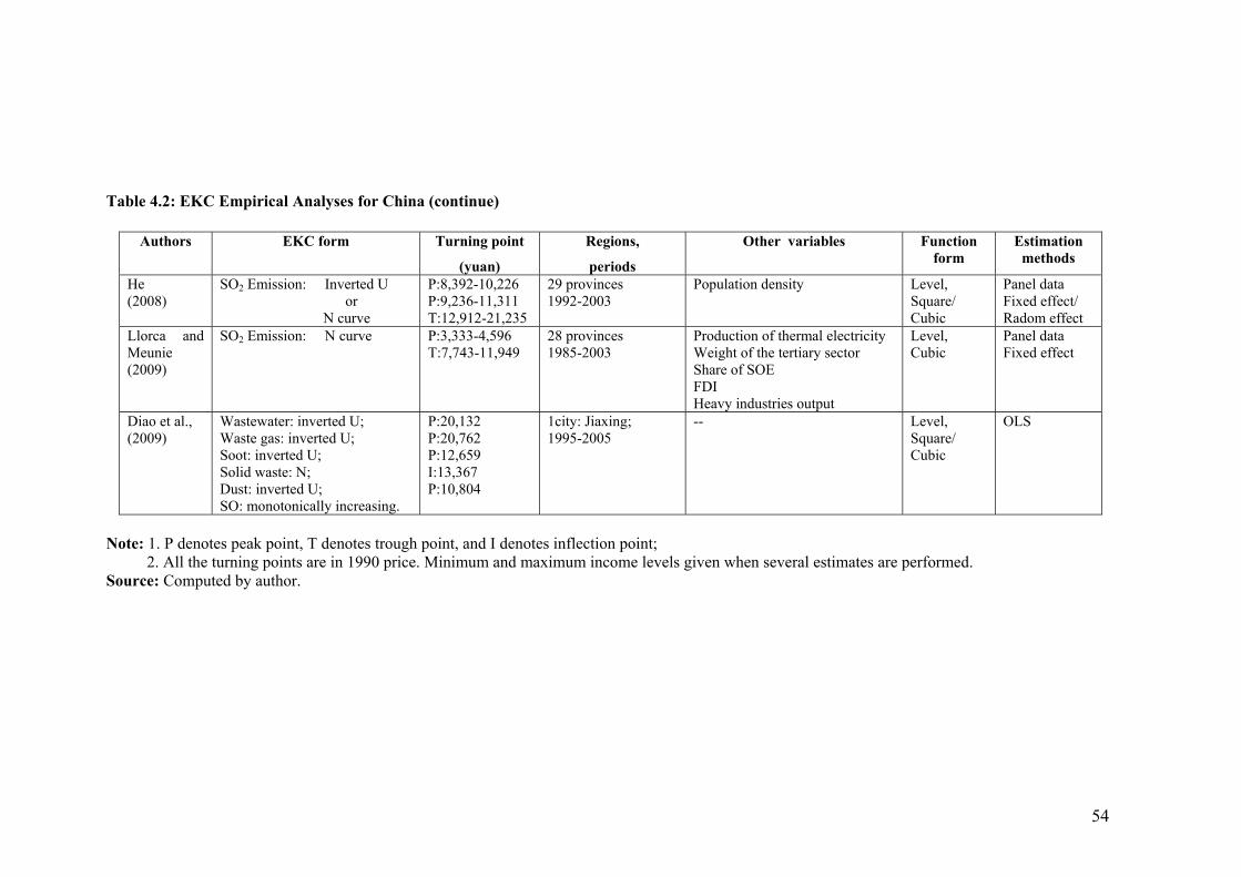
54
Table 4.2: EKC Empirical Analyses for China (continue)
Authors EKC form Turning point
(yuan)
Regions,
periods
Other variables Function form
Estimation methods
He (2008)
SO2 Emission: Inverted U or N curve
P:8,392-10,226 P:9,236-11,311 T:12,912-21,235
29 provinces 1992-2003
Population density
Level, Square/ Cubic
Panel data Fixed effect/ Radom effect
Llorca and Meunie (2009)
SO2 Emission: N curve
P:3,333-4,596 T:7,743-11,949
28 provinces 1985-2003
Production of thermal electricity Weight of the tertiary sector Share of SOE FDI Heavy industries output
Level, Cubic
Panel data Fixed effect
Diao et al., (2009)
Wastewater: inverted U; Waste gas: inverted U; Soot: inverted U; Solid waste: N; Dust: inverted U; SO: monotonically increasing.
P:20,132 P:20,762 P:12,659 I:13,367 P:10,804
1city: Jiaxing; 1995-2005
-- Level, Square/ Cubic
OLS
Note: 1. P denotes peak point, T denotes trough point, and I denotes inflection point; 2. All the turning points are in 1990 price. Minimum and maximum income levels given when several estimates are performed. Source: Computed by author.

55
4.5 Empirical Methodology and Data
As noted in the previous section, past researchers used different data sets (time series
data or panel data) and different EKC models (quadratic or cubic functions) to
investigate China’s economic growth and environmental quality and found mixed
results. This section introduces the empirical methodology and data which will be
used in our analysis.
4.5.1 Empirical Methodology
Panel data that have both time series and cross sections are common in economics.
Most of the recent studies of the Kuznets curve have used panel data because it
provides a lot of information about an economy and allows researchers great
flexibility in modelling differences in behaviour across individuals (Nikopour et al.,
2009). Provincial level panel data is used to analyse the relationship between
pollution emissions and income in China. There are two major advantages in using
within country data rather than cross-country data. First, it ensures a consistent
measurement of pollution, income, and policy. Second, although there are some
differences among Chinese provinces, the samples are more homogeneous in political
freedom, legal institution, cultural norms and corruption compared to cross country
data (Chintrakarn and Millimet, 2006).
The simple quadratic functions of the levels of income model are commonly used to
test the EKC (Selden and Song, 1994; Shukla and Parikh, 1996; Cole et al., 1997;
Kaufman et al., 1998; List and Gallet, 2000; Perman and Stern, 1999; Dinda et al.,
2000; Egli, 2002; Jiang et al., 2008; He, 2008; and Diao et al., 2009). In addition,
some studies (e.g. Panayotou, 1997; Gale and Mendez, 1998; Torras and Boyce, 1998;
List and Gallet, 2000; Barrett and Graddy, 2000; Harbaugh et al., 2000; Cole and
Elliott, 2003; Groot et al., 2004; Yap et al., 2007; and Llorca and Meunie, 2009),
including the original Grossman and Krueger (1991) paper, used a cubic EKC in
levels and found an N-shaped EKC. Therefore, in order to test for the possible re-
increasing or re-decreasing trends of the EKC after the dichotomy between economic
growth and pollution has been achieved, both quadratic and cubic EKC models are
estimated in this chapter as follows:

56
2
1 2it i t it it itE Y Yα μ β β ε= + + + + (1)
2 3
1 2 3it i t it it it itE Y Y Yα μ β β β ε= + + + + + (2)
i = 1, 2, …, 30,
t = 1, 2, …, 18, or 1990, 1991,…, 2007,
where i indexes provinces and t indexes time; Eit is one of the four pollutants
measured in per capita terms for province i at time t; Y is real GDP per capita for
province i at time t; β is the coefficient parameter; αi are cross-section effects; μt are
time effects; and εit is the error term assumed to be stationary. The intercept term is
assumed to be correlated with the explanatory variables and let the intercept vary
among provinces.
βs jointly defines the relationship per capita emissions and per capita GDP. Based on
the EKC model the three coefficients capture all the direct and indirect marginal
impact of economic development on the environment as measured by the level of per
capita emissions of a particular pollutant20. The turning point for the alternative
function is defined in Table 4.3.
Table 4.3: Types of Relationship between Environmental Quality and Economic Growth
China’s economic reform took a gradual approach (Jiang et al., 2008). The
development policies were set in the coastal provinces first and later shifted to the
central and western provinces (Table 4.4 lists provinces and municipalities that
belong to each region). Meanwhile, industrial relocation could occur between
20 In equation (1) (2), β1, β2 and β3 do not vary by province, implying an isomorphic EKC for all provinces.

57
developed and under-developed regions. More polluting industries moved inland
from the coastal region after reform. From 1990 to 2007 the average per capita GDP
for the coastal provinces increased from 2,545 yuan to 14,544 yuan, from 1,451 yuan
to 7,458 yuan for the central region, and from 1,207 yuan to 5,547 yuan21 for the
western provinces. There was a large disparity in growth among the regions and
therefore exploring whether the relationships between income and pollution vary by
region was worth.
Table 4.4: Regional Definitions
Region Coastal Central Western Provinces (municipalities)
Beijing Fujian Guangdong Guangxi Hainan Hebei Jiangsu Liaoning Shandong Shanghai Tianjin Zhejiang
Anhui Heilongjiang Henan Hubei Hunan Inner Mongolia Jiangxi Jilin Shanxi
Gansu Guizhou Ningxia Qinghai Shaanxi Sichuan Tibet Xinjiang Yunnan
The sample comprises 30 provinces\municipality\autonomous regions from 1990-
2007. Chongqing became a municipality directly under the jurisdiction of the central
government in 1996. In order to remain consistent, the relevant data for Chongqing
are added to those for Sichuan province. The relationship between four emissions of
industrial pollutants per capita and income per capita, based on available data, are
tested in this chapter. They are industrial SO2, industrial smoke, industrial dust, and
industrial COD. The emissions data are collected from the China Environmental
Yearbook over various years.
Population is the figure at the end of the year. GDP (in the current year) and the
general consumer price index (1990=100) data were obtained from various issues of
the China Statistical Yearbook. Yit is provincial GDP per capita, which is GDP at a
constant 1990 price divided by the population figure at the end of the year. The real
GDP per capita was chosen because it was a better proxy for income level.
21 Yuan is the unit name of Chinese currency, the renminbi. All the renminbi numbers have been adjusted to its 1990 value.
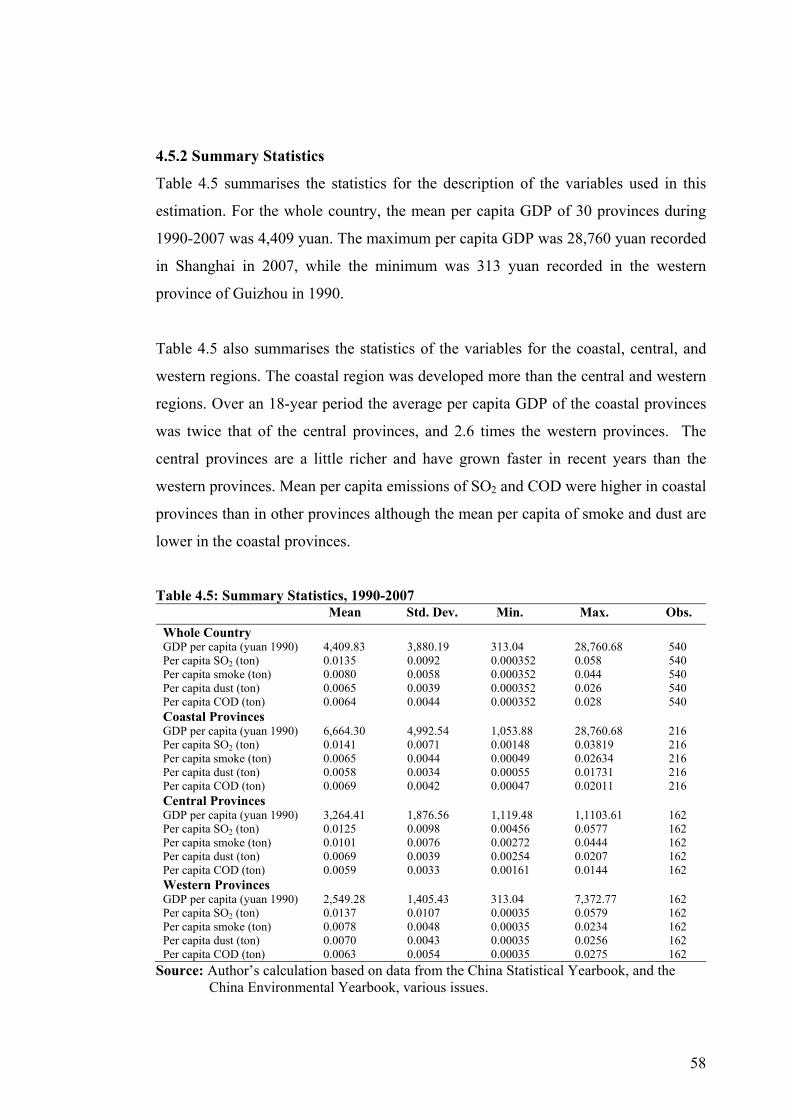
58
4.5.2 Summary Statistics
Table 4.5 summarises the statistics for the description of the variables used in this
estimation. For the whole country, the mean per capita GDP of 30 provinces during
1990-2007 was 4,409 yuan. The maximum per capita GDP was 28,760 yuan recorded
in Shanghai in 2007, while the minimum was 313 yuan recorded in the western
province of Guizhou in 1990.
Table 4.5 also summarises the statistics of the variables for the coastal, central, and
western regions. The coastal region was developed more than the central and western
regions. Over an 18-year period the average per capita GDP of the coastal provinces
was twice that of the central provinces, and 2.6 times the western provinces. The
central provinces are a little richer and have grown faster in recent years than the
western provinces. Mean per capita emissions of SO2 and COD were higher in coastal
provinces than in other provinces although the mean per capita of smoke and dust are
lower in the coastal provinces.
Table 4.5: Summary Statistics, 1990-2007 Mean Std. Dev. Min. Max. Obs. Whole Country GDP per capita (yuan 1990) Per capita SO2 (ton) Per capita smoke (ton) Per capita dust (ton) Per capita COD (ton) Coastal Provinces GDP per capita (yuan 1990) Per capita SO2 (ton) Per capita smoke (ton) Per capita dust (ton) Per capita COD (ton) Central Provinces GDP per capita (yuan 1990) Per capita SO2 (ton) Per capita smoke (ton) Per capita dust (ton) Per capita COD (ton) Western Provinces GDP per capita (yuan 1990) Per capita SO2 (ton) Per capita smoke (ton) Per capita dust (ton) Per capita COD (ton)
4,409.83 0.0135 0.0080 0.0065 0.0064 6,664.30 0.0141 0.0065 0.0058 0.0069 3,264.41 0.0125 0.0101 0.0069 0.0059 2,549.28 0.0137 0.0078 0.0070 0.0063
3,880.19 0.0092 0.0058 0.0039 0.0044 4,992.54 0.0071 0.0044 0.0034 0.0042 1,876.56 0.0098 0.0076 0.0039 0.0033 1,405.43 0.0107 0.0048 0.0043 0.0054
313.04 0.000352 0.000352 0.000352 0.000352 1,053.88 0.00148 0.00049 0.00055 0.00047 1,119.48 0.00456 0.00272 0.00254 0.00161 313.04 0.00035 0.00035 0.00035 0.00035
28,760.68 0.058 0.044 0.026 0.028 28,760.68 0.03819 0.02634 0.01731 0.02011 1,1103.61 0.0577 0.0444 0.0207 0.0144 7,372.77 0.0579 0.0234 0.0256 0.0275
540 540 540 540 540 216 216 216 216 216 162 162 162 162 162 162 162 162 162 162
Source: Author’s calculation based on data from the China Statistical Yearbook, and the China Environmental Yearbook, various issues.

59
Figure 4.3 presents the trends of four industrial pollutants over time. Per capita
emissions of SO2 first increased and then peaked in 1997. From 1998 it slowly
dropped but went up again after 2002. At the same time, per capita emissions of COD,
smoke, and dust show a slow but significant decline. This decline in industrial
emissions was confirmed to the ten-year environmental review issued by MEP (2006),
and was also noted by the WTO (2006) and the OECD (2005).
Figure 4.3: Per Capita Emissions in China, 1990-2007
0
0.005
0.01
0.015
0.02
1990 1991 1992 1993 1994 1995 1996 1997 1998 1999 2000 2001 2002 2003 2004 2005 2006 2007
so2 cod smoke dust
Source: Author’s calculation based on data from the China Statistical Yearbook, and the China Environmental Yearbook, various issues.
4.6 Empirical Results
Panel data models examine OLS (Ordinary Least Squares) and also fixed effects and
random effects. To obtain an appropriate estimation of our model it is necessary to
proceed to the following tests. The F test relates to testing OLS versus fixed effects. It
is a test for the joint significance of the provinces dummy variables. If it is significant,
we reject the null hypothesis that the intercept parameters for all provinces are equal.
We conclude that there are differences in provincial intercepts and the fixed effects
model was appropriate.
The Hausman specification test compares the fixed versus random effects under the
null hypothesis that the individual effects are uncorrelated with the other regressors in
the model, namely, that the random effects would be consistent and efficient
(Hausman, 1978). If correlated (the null hypothesis is rejected), a random effect
model produces biased estimators, violating one of the Gauss-Markov assumptions;
so a fixed effect model is preferred.

60
4.6.1 Whole Country
Table 4.6 reports the estimation results of equations (1) 22 for each of the four
pollutants. The null hypothesis of the homogenous province effect is strongly rejected
at a wide margin (see F-test) for every pollutant. This evidence suggests that OLS
estimators are inefficient and may yield biased estimates. In addition, the results of
the Hausman test for selecting between random or fixed effects estimation reject the
assumption made by the random effects model. Therefore, OLS and random effects
estimations are not reported. The province-specification fixed effect accounts for the
time-invariant factors such as resource endowment which are unique to each province,
while the time-specification fixed effect captures the shocks such as changes in
environmental regulation, technological progress, or shift in preferences, which are
common to all the provinces in each year. The adjusted R2 values of these models
range from 0.65 to 0.85, which suggests that the estimated function performs well in
terms of goodness-of-fit statistics.
Table 4.6: Estimates for 30 Provinces SO2 Smoke Dust COD
Constant 0.0124***
(10.642) 0.0093***
(13.097) 0.0086***
(15.9609) 0.0092*** (30.88)
Y 5.93e-07*
(1.8614) -2.43e-07 (-1.1499)
-4.78e-07*** (-3.1986)
-7.01e-07*** (-9.0635)
Y2 -4.65e-11***
(-5.4694) -8.64e-12 (-1.2447)
9.39e-13 (0.2373)
9.26e-12*** (5.8005)
Turning point 6,376.34 -- -- -- Adj. R2 0.8495 0.7495 0.6516 0.8579
F-statistic 64.40*** 34.59*** 21.99*** 68.83***
Hausman 8.40** 12.81*** 9.92*** 10.74***
No. of Obs. 540 540 540 540 Shape of curve Inverted-U -- Linear U
Notes: 1.The values in parenthesis are the t-statistics for variables; 2. * indicates significant at 10% level, ** for 5%, and *** for 1%; 3. Turning points refer to income per capita at 1990 constant price. Source: Computed by the Author.
22 For whole country, we focus on the turning point of Inverted-U curve for further analysis (detailed in Chapter Five). Therefore, only the results of quadratic EKC model are discussed here. However, we also tried cubic model similar as in the literature of Lorca and Meunie (2009) and Yap et al. (2007), we found N-shaped curves for SO2, smoke and dust, and inverted-N shape curve for COD. The peak turning points for the N-shaped curves for smoke and dust are 6,306 yuan and 5,447 yuan respectively. The trough turning points often fall far out of the sample.

61
For per capita SO2, β1 is positive significantly at the10% level and β2 is negative
significantly at the1% level, which suggests an inverted-U shaped EKC (see Table
4.6, and Figure 4.4). Depending on the provincial and time fixed effects, the per
capita SO2 starts to decline when per capita GDP achieves 6,376.34 yuan. Most
coastal provinces except Hainan and Guangxi were on the right side of the turning
point by the end of 2007. Six central provinces (Heilongjiang and Inner Mongolia in
2005, Jilin and Shanxi in 2006, Henan and Hubei in 2007) had just recently reached
this level but only Xinjiang province in the western region had passed this turning
point in 2006.
Figure 4.4: The EKC for SO2: Whole Country. (Quadratic Form) SO2 per capita
6,376 yuan GDP per capita
For the emissions of dust per capita, a monotonically decreasing relationship is found
with β1 is negative significantly, suggesting that dust declines with income. For per
capita COD, with β1 negative and β2 positive, a U-shaped relationship between per
capita COD and per capita GDP is suggested, with the turning point at 37,900 yuan.
Every province is located at the left side of curve.
17/30 provinces

62
4.6.2 Coastal Region
The estimated results for the coastal region are presented in Table 4.7. The fixed
effect model based on the F-test and Hausman tests is adopted.
Table 4.7: Estimates for Provinces in the Coastal Region SO2 Smoke Dust COD
Squared Cubic Squared Cubic Squared Cubic Squared Cubic 0.0166*** 0.0051 ** 0.0115*** 0.0052*** 0.0101*** 0.0062*** 0.0109*** 0.0121***
Constant (15.44) (2.2769) (11.002) (3.1712) (16.9395) (4.5687) (18.9387) (9.9388)
-1.12e-07 3.14e-06*** -7.55e-07 1.04e-06** -7.38e-07*** 3.69e-07 -6.90e-07*** -9.98e-07*** Y (-0.4649) (4.4813) (-0.5558) (2.1442) (-5.8881) (0.9683) (-6.5964) (-2.6282)
-2.55e-10*** -2.43e-10*** 7.06e-13 -1.20e-10*** 8.38e-12** -6.55e-11** 6.69e-12*** 2.75e-11
Y2 (-2.8185) (-4.5169) (0.1114) (-3.1693) (2.258) (-2.5189) (2.9894) (0.9755)
4.79e-15*** 2.65e-15*** 1.63e-15*** -4.53e-16 Y3
--
(3.9523)
--
(3.0521)
--
(2.7788)
--
(-0.7343)
Turning point (P)
--
8,700
--
5,240
--
--
--
--
Turning point (T) -- 25,100 -- 24,900 44,000 -- 51,600 --
Adj. R2 0.8182 0.8353 0.749 0.7621 0.6869 0.6947 0.8519 0.8516
F-statistic 33.25*** 36.18*** 22.38*** 23.21*** 16.72*** 16.78*** 42.24*** 40.81***
Hausman 5.15* 6.02* 22.4*** 37.8*** 4.23 5.01 3.12 5.12
No. of Obs. 216 216 216 216 216 216 216 216
Shape-of Linear
curve
-- N
(Decreasing)
N U -- U --
Notes: 1.The values in parenthesis are the t-statistics for variables; 2. * indicates significant at 10% level, ** for 5%, and *** for 1%; 3. Turning points refer to income per capita at 1990 constant price. Source: Computed by the Author.
The EKC for the coastal region is not found. The relationship between SO2 and
income per capita is an N-shaped curve (see Table 4.7 and Figure 4.5). A per capita
SO2 emissions peak is seen at a per capita income of 8,700 yuan. According to the
estimated regression, SO2 per capita emissions are expected to re-increase as per
capita income increases up to 25,100 yuan. By the end of 2007 most of coastal
provinces, except Guangxi, Hainan, Hebei, and Liaoning, was on the downward slope
of the curve but Beijing and Shanghai achieved the trough turning point (Beijing in
2007, and Shanghai in 2006).

63
Figure 4.5: The EKC for SO2: Coastal Region. (Cubic Form) SO2 per capita
8,700 yuan 25,100 yuan GDP per capita
The relationship between smoke and income per capita is also an N-shaped curve (see
Table 4.7 and Figure 4.6). The whole coastal region has passed the peak turning point
(5,240 yuan per capita), and only Beijing and Shanghai reached the trough turning
point.
Figure 4.6: The EKC for Smoke: Coastal Region. (Cubic Form) Smoke per capita
5,240 yuan 24,900 yuan GDP per capita
The relationships between dust/COD and income per capita are a U-shaped curve
with the turning point at 44,000 yuan and 51,600 yuan respectively. The whole region
is on the left side of the curve, and a long way behind the turning points. If we take
the 12 provinces\municipalities as a whole, the emissions of SO2 and smoke are
becoming more and more severe.
Only Shanghai and Beijing
17/19 provinces
Only Shanghai and Beijing
13/19 provinces
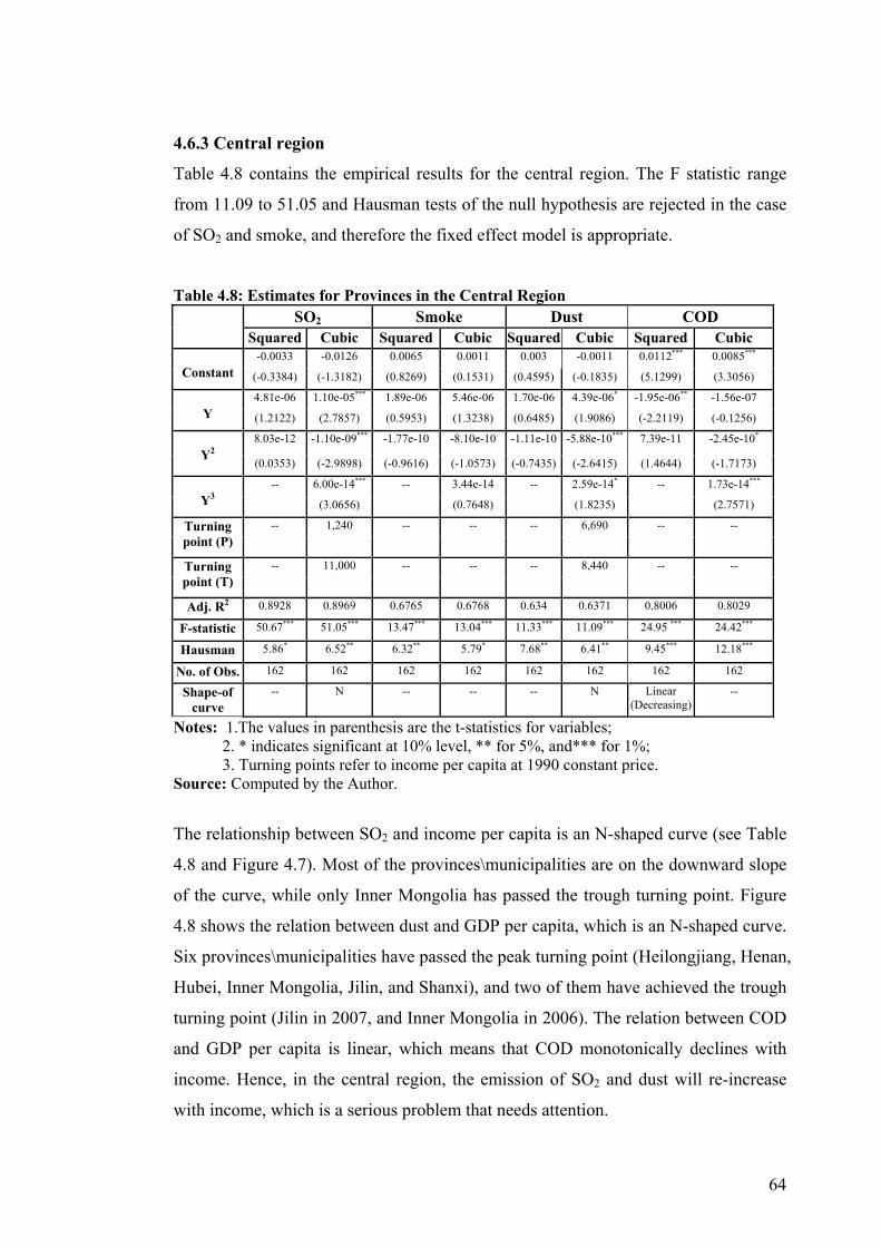
64
4.6.3 Central region
Table 4.8 contains the empirical results for the central region. The F statistic range
from 11.09 to 51.05 and Hausman tests of the null hypothesis are rejected in the case
of SO2 and smoke, and therefore the fixed effect model is appropriate.
Table 4.8: Estimates for Provinces in the Central Region SO2 Smoke Dust COD
Squared Cubic Squared Cubic Squared Cubic Squared Cubic -0.0033 -0.0126 0.0065 0.0011 0.003 -0.0011 0.0112*** 0.0085***
Constant (-0.3384) (-1.3182) (0.8269) (0.1531) (0.4595) (-0.1835) (5.1299) (3.3056)
4.81e-06 1.10e-05*** 1.89e-06 5.46e-06 1.70e-06 4.39e-06* -1.95e-06** -1.56e-07 Y (1.2122) (2.7857) (0.5953) (1.3238) (0.6485) (1.9086) (-2.2119) (-0.1256)
8.03e-12 -1.10e-09*** -1.77e-10 -8.10e-10 -1.11e-10 -5.88e-10*** 7.39e-11 -2.45e-10* Y2
(0.0353) (-2.9898) (-0.9616) (-1.0573) (-0.7435) (-2.6415) (1.4644) (-1.7173)
6.00e-14*** 3.44e-14 2.59e-14* 1.73e-14*** Y3
--
(3.0656)
--
(0.7648)
--
(1.8235)
--
(2.7571)
Turning point (P)
-- 1,240 -- -- -- 6,690 -- --
Turning point (T)
-- 11,000 -- -- -- 8,440 -- --
Adj. R2 0.8928 0.8969 0.6765 0.6768 0.634 0.6371 0.8006 0.8029
F-statistic 50.67*** 51.05*** 13.47*** 13.04*** 11.33*** 11.09*** 24.95 *** 24.42***
Hausman 5.86* 6.52** 6.32** 5.79* 7.68** 6.41** 9.45*** 12.18***
No. of Obs. 162 162 162 162 162 162 162 162
Shape-of curve
-- N -- -- -- N Linear (Decreasing)
--
Notes: 1.The values in parenthesis are the t-statistics for variables; 2. * indicates significant at 10% level, ** for 5%, and*** for 1%; 3. Turning points refer to income per capita at 1990 constant price. Source: Computed by the Author.
The relationship between SO2 and income per capita is an N-shaped curve (see Table
4.8 and Figure 4.7). Most of the provinces\municipalities are on the downward slope
of the curve, while only Inner Mongolia has passed the trough turning point. Figure
4.8 shows the relation between dust and GDP per capita, which is an N-shaped curve.
Six provinces\municipalities have passed the peak turning point (Heilongjiang, Henan,
Hubei, Inner Mongolia, Jilin, and Shanxi), and two of them have achieved the trough
turning point (Jilin in 2007, and Inner Mongolia in 2006). The relation between COD
and GDP per capita is linear, which means that COD monotonically declines with
income. Hence, in the central region, the emission of SO2 and dust will re-increase
with income, which is a serious problem that needs attention.

65
Figure 4.7: The EKC for SO2: Central Region. (Cubic Form) SO2 per capita
1,240 yuan 11,000 yuan GDP per capita
Figure 4.8: The EKC for Dust: Central Region. (Cubic Form) Dust per capita
6,690 yuan 8,440 yuan GDP per capita
2/9 provinces
4/9 provinces
Only Inner Mongolia
8/9 provinces

66
4.6.4 Western Region
Table 4.9 presents the results for the western region. The fixed effect model is also
used to test the relationship between GDP per capita and pollution emissions per
capita in the western region.
Table 4.9: Estimates for Provinces in the Western Region SO2 Smoke Dust COD
Squared Cubic Squared Cubic Squared Cubic Squared Cubic 0.0124*** 0.0198*** 0.0102*** 0.0062** 0.0092*** 0.0102*** 0.0099*** 0.0054***
Constant (2.8571) (5.1517) (5.7282) (2.0886) (4.2221) (2.6632) (10.0344) (3.8957)
1.48e-07 -6.30e-06** -1.36e-06 2.10e-06 -1.74e-06 -2.55e-06 -1.68e-06 2.30e-06** Y (0.0657) (-2.3189) (-1.3806) (0.8845) (1.51) (-0.9280) (-1.3203) (2.3125)
1.01e-10 1.73e-09*** 1.27e-10 -7.46e-10 2.63e-10*** 4.69e-10 7.08e-11 -9.34e-10*** Y2 (0.6086) (2.6189) (1.3825) (-1.3389) (2.8199) (0.8324) (1.4589) (-3.4734)
-1.35e-13** 7.24e-14 -1.71e-14 8.33e-14*** Y3
--
(-2.2386)
--
(1.6472)
--
(-0.4101)
--
(3.3361)
Turning point (P) -- 5,910 -- -- -- -- -- 1,150
Turning point (T) -- 2,630 -- -- -- -- -- 5,920
Adj. R2 0.8901 0.8915 0.8809 0.9036 0.6368 0.6343 0.8707 0.873
F-statistic 49.28*** 48.22*** 45.15*** 44.50*** 11.45*** 10.97*** 41.17*** 40.54***
Hausman 8.53** 10.21** 5.01 2.33 7.26** 8.14** 10.22*** 14.07***
No. of Obs. 162 162 162 162 162 162 162 162
Shape-of curve
-- Inverted N -- -- -- -- -- N
Notes: 1.The values in parenthesis are the t-statistics for variables; 2. * indicates significant at 10% level, ** for 5%, and*** for 1%; 3. Turning points refer to income per capita at 1990 constant price. Source: Computed by the Author.
There is an N-shaped curve between COD and income per capita (see Table 4.9 and
Figure 4.9). The whole region has passed the peak turning point but five of them
recently reached the trough turning point (Sichuan, Qinghai, Ningxia and Shaanxi in
2007; Xinjiang in 2005). So, the emissions of COD in the western region keeping
rising with income which means environment will worse. An inverted N-shaped
curve exists between SO2 and income per capita. The whole region has passed the
trough turning point, and five of them achieved the peak turning point (Ningxia,
Qinghai, Shaanxi, and Sichuan in 2007; Xinjiang in 2005), which means the
emissions of SO2 are re-decreasing with income.
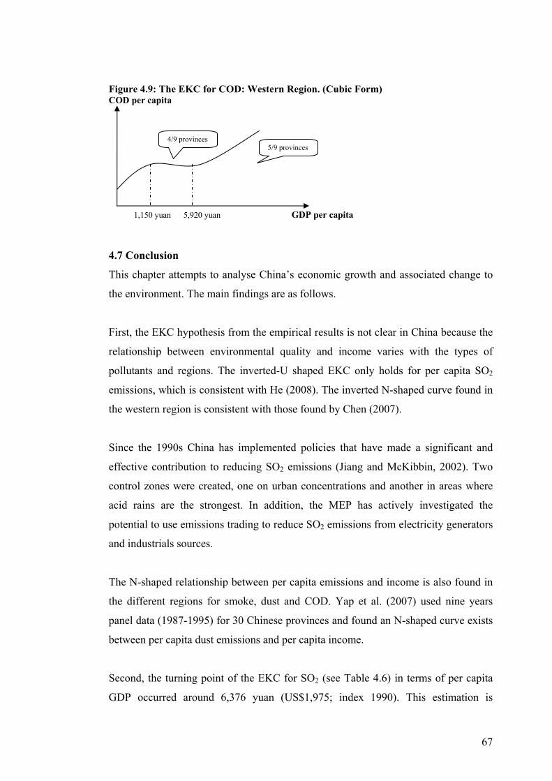
67
Figure 4.9: The EKC for COD: Western Region. (Cubic Form) COD per capita
1,150 yuan 5,920 yuan GDP per capita
4.7 Conclusion
This chapter attempts to analyse China’s economic growth and associated change to
the environment. The main findings are as follows.
First, the EKC hypothesis from the empirical results is not clear in China because the
relationship between environmental quality and income varies with the types of
pollutants and regions. The inverted-U shaped EKC only holds for per capita SO2
emissions, which is consistent with He (2008). The inverted N-shaped curve found in
the western region is consistent with those found by Chen (2007).
Since the 1990s China has implemented policies that have made a significant and
effective contribution to reducing SO2 emissions (Jiang and McKibbin, 2002). Two
control zones were created, one on urban concentrations and another in areas where
acid rains are the strongest. In addition, the MEP has actively investigated the
potential to use emissions trading to reduce SO2 emissions from electricity generators
and industrials sources.
The N-shaped relationship between per capita emissions and income is also found in
the different regions for smoke, dust and COD. Yap et al. (2007) used nine years
panel data (1987-1995) for 30 Chinese provinces and found an N-shaped curve exists
between per capita dust emissions and per capita income.
Second, the turning point of the EKC for SO2 (see Table 4.6) in terms of per capita
GDP occurred around 6,376 yuan (US$1,975; index 1990). This estimation is
5/9 provinces 4/9 provinces

68
consistent with the estimations of Llorca and Meunie (2009) (3,333-4,596 yuan), and
He (2008) (8,392-10,226 yuan). However, Panayotou (1993) used data from 55
developed and developing countries from 1987 to 1988 and then estimated that the
turning point of the SO2 emissions into the air would occur when per capita GDP
reached US$3,13723 (index 1990). China entered this decreasing part of the EKC at
an earlier stage than the countries with those experiences. The reason may be that
China has learned how other countries manage their environmental problems. As
Grossman (1995, p.44) pointed out “the low-income countries of today have a unique
opportunity to learn from this history and thereby avoid some of the mistakes of
earlier growth episodes.”
Third, the results of comparing the turning points for SO2 show that the poor central
and western regions appear to have turning points that occur at lower income levels
than the coastal region. This suggests that technology diffusion, leapfrogging, and
institution imitation through learning among regions at different developmental stages
may have played a part in shaping the relationship between economic growth and
environmental sustainability (Jiang et al., 2008). These may encourage the less
developed regions to use cleaner technologies and institute better regulatory
frameworks for environmental protection at a lower income level.
Most studies on the relationship between environmental quality and income,
especially the EKC hypothesis, commonly conclude that economic growth may
spontaneously resolve the environmental problem. The limitation of EKC is that it
ignores the factors influencing environmental quality other than income (Zhang,
2004). The series of human activities usually affect the shape of EKC and the turning
point. Several measures could be taken to decrease environmental degradation and
make the turning point come earlier. First, using an advanced technological process to
reduce the volume of pollutants emitted during production; second, the government
strengthens propaganda against pollution and continue to increase its investment in
environmental protection, and third, the government should enforce their
environmental laws and policies.
23 See Stern, 2004.

69
This chapter only considers the effects of income on the environment, and omits the
function of trade on economic growth and the environment. The next chapter attempts
to explain the link between trade, economic growth, and the environment using a
more sophisticated simultaneous model.

70
CHAPTER FIVE
TRADE LIBERALISATION AND THE ENVIRONMENT:
Evidence from China’s Industrial Sector
5.1 Introduction
China has embraced the trade liberalisation process through a significant reduction of
tariffs and non-tariff barriers (Zhang et al., 1999), and the results have been
spectacular (Chai, 2002). The share of exports and imports in China’s GDP has shot
up from 11% in 1979 to 85% in 2007. Trade liberalisation accompanied by
liberalisation of foreign direct investment regimes and economic reform enabled
China to achieve a double-digit rate of growth during the period 1979-2007. However,
there has been an increasing concern over the potentially negative impacts of trade
liberalisation, particularly on the environmental and natural resources where trade has
grown most rapidly.
The purpose of this chapter is to identify the trade related environmental performance
of China’s industrial sector during the period 1990-2007. The following hypothesis
will be tested for this purpose: trade liberalisation has a short term negative effect on
the environment but a long term positive effect will occur provided that externalities
can be internalised with the rise in income and new technology.
The rest of this chapter is outlined as follows: section 5.2 presents the relationship
between trade and environment, section 5.3 introduces the model and data, section
5.4 reports the empirical results, and section 5.5 concludes.
5.2 The Relationship between Trade and the Environment
The linkage between trade liberalisation and the environment has become an
important policy issue. It was commonly assumed by economists and
environmentalists alike that greater economic openness would lead to increased
pollution in developing countries, which means trade liberalisation would increase
environmental degradation in developing countries. One common concern among
environmentalists was that liberalised trade regimes and market-driven exchange
rates would increase the incentives for export and subsequently lead to a greater
71
exploitation of natural resources (Mukhopadhyay and Chakraborty, 2005). Secondly,
trade between countries with differing levels of environmental regulations could lead
dirty industry to concentrate in the nations where regulations are lax. Developing
countries are frequently thought to have less stringent environmental regulations than
developed countries. Therefore, through free trade developing countries might have a
comparative advantage in industries that are associated with relatively large
environmental externalities (Baumol and Oates, 1988; Seibert, 1981). In addition,
free trade would increase industrial pollution in developing countries through
competitive pressure to further reduce their environmental standards.
There are two conflicting hypotheses emerging from this debate. The first is known
as the pollution heaven hypothesis which suggests that pollution intensive industry
tends to migrate towards countries with weaker environmental regulations. Because
economic growth is the key objective of these countries, and government would use
relatively weak environmental policies to either attract these pollution intensive
industries by foreign direct investment from developed countries which have
relatively stringent environmental regulations, or raise the competitiveness of
domestic pollution intensive industries due to relatively lower prices (Shen, 2008).
According to this hypothesis the developing countries possess a comparative
advantage in pollution intensive production. Although some analyses support this
hypothesis (such as Low and Yeats, 1992; Xing and Kolstad, 2002; and Cole, 2004),
most empirical studies do not (Eskeland and Harrison, 2003; Mani, 1999; Neumater,
2001; and Wheeler, 2001), arguing that environmental regulations are a variable
conditioning the international location of pollution intensive industries.
An alternative factor endowment hypothesis asserts that in free trade the differences
in endowments determine trade between two countries (Dinda, 2005). This
hypothesis predicts that relatively capital-abundant countries export pollution-
intensive goods since most are capital-intensive (Shen, 2008). Developed countries
are typically well endowed with capital. Therefore, this hypothesis says that
developed countries specialise in pollution-intensive goods and export them, which
means developed countries would be more polluted than developing countries. Thus,
the pollution heaven hypothesis is in direct conflict with the factor endowment
72
hypothesis. Both hypotheses were tested for China by Shen (2008). Shen found that
the evidence for the factor endowment hypothesis existed in most of the pollutants
but there was no evidence for the pollution heaven hypothesis.
A standard approach for thinking about trade and the environment was proposed by
Grossman and Kruger (1991). They stated that trade liberalisation may theoretically
affect the environment through a variety of channels such as scale, composition, and
technique effects.
The scale effect refers to an increase in the size of an economy that results from trade
liberalisation induced increases in market access. Ceteris paribus, the scale effect
likely leads to rising pollution emissions. However, although free trade and increased
production levels might be accompanied by adverse environmental effects, a number
of other factors make it difficult to isolate the pure scale effects and identify a strong
pattern in the commonly assumed detrimental relationship between increased
economic activity and environmental performance (Kirkpatrick and Scrieciu, 2008).
Environmentally beneficial income effects might arise when augmented financial
capacity supplies more resources for environmental protection (supply-side effects)
and fosters greater demand for environmental quality (demand-side effects) (Esty and
Ivanova, 2003). Nevertheless, although it may be difficult to isolate the pure scale
effect, it is increasingly acknowledged that the scale of production and consumption
effects are having a net negative impact on the environment, particularly with
reference to climate change and global warming (IPCC, 2007; and Stern, 2007)
The second is concerned with the technique effect. Trade liberalisation can lead to a
change in the environmental effects of the methods of production. Openness may spur
more environmentally friendly technological innovation which has a positive effect
on both the economy and the environment (Kirkpatrick and Scrieciu, 2008). Similarly,
trade liberalisation can enhance access to environmental know-how and technology,
either through imports of environmental goods and services or through cleaner
production techniques embodied in foreign direct investment (OECD, 2000; and
Hoekman et al., 2002).
73
Finally, the composition effect states that accompanying trade liberalisation, the
industrial structure of an economy will change. This change may have either a
positive or negative impact on the environment. The impact is positive if a country
has a comparative advantage in the production of less pollution-intensive industries.
In addition, income growth increases demand for relatively cleaner goods, which
causes the share of pollution-intensive goods in output to fall, which reduces
emissions. As a result, its output composition will become cleaner after trade
liberalisation. By way of contrast, a negative composition effect refers to the fact that
trade liberalisation may result in a country specialising in pollution-intensive
industries due to its factor endowments.
It is clear from the above that the effect of trade liberalisation on the environment is
theoretically ambiguous because these effects may work in opposite directions. The
net effect of trade liberalisation on the environment depends on whether the positive
composition and technical effects are larger or smaller than the negative composition
and scale effects. Dean (2002) stated that at relative low incomes country the scale
effect outweighs the positive composition and technique effects. Thus, as a poor
country begins to grow, it sees a net increase in environmental damage but over time,
income reaches some critical level and the latter two effects outweigh the former.
Growth then leads to a net reduction in environmental damage.
5.3 Literature Review: China
With regards to the relative size of the composition, technical, and scale effects, there
have been a few studies in this area on the contribution of China. From the literatures
we can see that trade liberalisation almost certainly leads to a complex combination
of both positive and negative effects on the environment. The net effect will vary by
pollutants and time.
Dean (2002) investigated the impact of trade and growth on the environment in China.
Dean examined water pollution from 1987 to 1995. Her approach was to create a
simultaneous-equations system which incorporated the multiple effects of trade
liberalisation. There are two reasons why Dean chose China. First, China placed
water pollution levies on firms as early as 1981, and Dean’s evidence examining

74
pollution at the provincial level shows that discharge intensity fell dramatically in
most provinces during the period examined. However, Dean also noted that the
amount of wastewater discharge rose in most provinces. Second, China was quite
protectionist in its trade policies until about 1992 when it embarked upon a rather
clear shift toward trade liberalisation.
Dean relied on the acceptance which was to consider trade as having three component
effects on pollution the scale effect, the technique effect, and the composition effect.
Therefore, pollution might increase through the scale effect simply as an economy
grows. More production requires more factor inputs and more pollution results.
However, trade can lead to promotion of cleaner techniques in production processes
that reduce emissions (the technique effect). The composition effect captures at least
part of the pollution haven hypothesis. Even if this hypothesis fails the composition
effect could result in other ways, for instance income increases it is likely that
demand for cleaner goods increases which might pressure firms into shifting
production and therefore reducing pollution, and as developed countries become
stricter with pollution policy, developing nations may focus more on promoting dirty
industries.
Dean attempted to disentangle these three effects using a reduced-form HO trade
model and assuming that the environment is a factor of production. In that case trade
directly affects the environment, depending on the type of output (the composition
effect) and indirectly through income growth (the scale effect increases pollution
while the technique effect reduces it).
She concluded by stating that her model explains Chinese income growth quite well
and Chinese emissions growth moderately well. Most importantly her results do seem
to capture the multiple effects of trade on pollution. The composition effect was
documented in that increases in the terms of trade seem to lead to more pollution. The
positive impact of the technique effect also seems clear; most provinces have worked
to clean up their water as trade-induced income increases have occurred. Therefore,
Dean stated that trade liberalisation has a beneficial environmental impact, although
the positive income effect outweighs the negative terms of trade effect.

75
Chai (2002) focussed on the manufacturing sector to assess the environmental impact
of trade liberalisation in China. She found that China’s experience with the trade
liberalisation-environment nexus was consistent with international evidence. On one
hand, trade liberalisation has had various positive effects on the environment. Firstly,
it promoted specialisation in areas of comparative advantage. Secondly, it allowed
China to access and adopt the best international practices in pollution abatement
technology. Thirdly, it enabled China to transfer environmental costs to other
countries. On the other hand these positive effects were overwhelmed by a negative
scale effect. Finally, Chai concluded by saying that if China is to prevent pollution
from reaching a critical threshold, environmental regulations need to be tightened.
Shen (2008) is related in many ways to Dean’s paper. For the same purpose, he
adopted the methodology provided by Antweiler et al. (2001) to exam whether the
composition effects arising from increasing trade originate due to differences in
capital-labour endowment and/or differences in environmental regulations
accompanied by income growth. Shen carried Dean’s approach a step further in that
an effort was made to identify the three effects. Using provincial data from 1993 to
2002 the results show evidence that the factor endowment hypotheses was found in
most pollutants (SO2, dust, COD, and arsenic); while there seemed to be no evidence
of the pollution heaven hypotheses. Shen then combined all the effects and found that
for SO2, and Dust, an increase in trade leads to more emissions and for COD, arsenic,
and cadmium, trade liberalisation decreases emissions.
In a recent working paper, Dean and Lovely (2008) calculated and tracked the
pollution content of China’s export and import bundles from 1995 to 2005. Their
calculations relied on official Chinese measurements of direct emissions of four
pollutants from about 30 Chinese industries. They found that as China’s trade has
grown the pollution intensity of almost every sector had fallen in terms of water
pollution (measured by COD) and air pollution (measured by SO2, smoke or dust) in
2004. This finding suggests that China has benefited from a positive “technique
effect” as emissions per real yuan of output have fallen across a wide range of
industries.
76
Dean and Lovely (2008) also revealed that China’s major exporting industries are not
highly polluting, and that the export bundle is shifting towards relatively cleaner
sectors over time. In 1995, textiles and apparel accounted for the largest shares of
Chinese exports to the world but they fell by about a third over the following decade.
Office and computing machinery and communications equipment, in contrast, were
the fastest growing exports and accounted for the largest export share in 2005. What
was striking is that these growing sectors are cleaner than textiles and apparel; indeed,
they are among the cleanest manufacturing sectors by the available measures of air
and water pollution. The most polluting sectors, such as paper and non-metallic
minerals, have in fact very low and declining shares in China’s manufacturing exports.
Linking industrial pollution intensities to detailed trade statistics from China Customs,
they found that, contrary to popular expectations, China’s exports are less water
pollution intensive and generally less air pollution intensive than Chinese import-
competing industries. Moreover, both Chinese exports and imports are becoming
cleaner over time. Part of this trend reflects changes in the composition of the trade
bundle, as noted above. However, the evidence suggests that most of the fall in the
pollution content of China’s trade was due to changes in industrial pollution
intensities rather than in trade patterns. This latter finding has important implications
as it suggests that the downward trend is not dependent on relationships with
particular trade patterns.
Table 5.1 summarises the literatures mentioned above. Where possible the results
were grouped into scale, technique, and composition effects. The scale effect has
consistently been found to increase pollution. Except for Dean (2002), the
composition effect of production tends to shift towards cleaner goods in China.
Overall, some pollutants were estimated to decrease with trade liberalisation whereas
others increased. Chua (1999) argued that any increases in pollution caused by trade
liberalisation were small compared to the increases attributed to growth and structural
changes that would have occurred even without trade liberalisation. Thus, the fear
that trade liberalisation will be detrimental to China’s environment is not borne out.

77
Table 5.1: Summary of Estimations on the Impact of Trade Liberalisation on the Environment
Author and pollutant Scale Technique Composition Net effect Dean (2002) + COD (Technique effect dominates) - Good Chai (2002) Cost Water pollution - + + (Scale effect out- Air pollution - + + weights composition Solid waste pollution - + + and technique effects)
Shen (2008) No decomposition between scale and technique effects - Air pollutant (Scale effect dominates technique) + Cost (SO2, Dust) + Water pollutant (Technique effect dominates scale) + Good (COD,Arsenic,Cadmium)
Dean and Lovely (2008) Water and Air pollutant NA + + Good Source: Author’s compiled.
5.4 Model Specification and Data Description
5.4.1 Model Specification
Although in many theoretical models pollution is assumed as both an input and by
product of production, these studies (e.g. Chai, 2002; Shen, 2008; Dean and Lovely,
2008) are based on a single polynomial equation where there is no feedback from
pollution to trade liberalisation, and therefore pollution is viewed only as the outcome
of free trade. The validity of ignoring this feedback effect should depend on that there
is no simultaneous relationship between these two variables. However, as we know,
trade liberalisation and the environmental quality are jointly determined, and
estimating the relationship only by a single polynomial equation might probably
produce biased and inconsistent estimates. From this view, it is more appropriate to
use a simultaneous equations model for the estimation. However, except Dean (2002),
there are seldom empirical studies that estimate the impact of trade liberalisation on
the environment by using simultaneous equations model.
The model employed in this analysis is similar to the one developed by Dean (2002).
Since the methodology of her study is central to this article, a brief outline of the
model is to be provided here.

78
5.4.1.1 Income Equation
Assume in a perfect competitive market with fully employed factors, a small open
economy24 produces two types of goods, dirty (X1) and clean (X2). There is no trans-
border pollution or consumption pollution so all emissions are generated by
production. To consider the environment as a factor of production, Lopez (1994) and
Dean (2002) pointed out that total industry output is also a function of the
environment factor of production. Therefore, production in each sector is a function
of the restrictiveness of the trade regime (T), the stock of conventional factors of
production, capital (Kj) and labour force (Lj), and the ability to generate
environmental damage (Ej).
( ) [ ( , ), ]i j j j jX A T h F L K E= (1)
where ( )h ⋅ is increasing and concave in ( )F ⋅ and in Ej and is characterised by constant
returns to scale in Lj, Kj, and Ej (j=1, 2). F(·) is an aggregator of the stock of
conventional factors. Factor productivity (A) is assumed to be a function of the limit
control of the trade regime (T). Increased openness is assumed to lead to higher total
factor productivity ( ' 0A < ) (Dean, 2002).
The specification (1) assumes a weak separability between the conventional factors of
production and the environmental factor, which means that the marginal rate of
technical substitution between capital and labour is assumed to be independent of the
level of pollution. Weak separability is a condition for the production function
defined only in terms of conventional factors of production to make sense when
factors other than the conventional ones change. Moreover, it simplifies the algebra
substantially by allowing for consideration of the interactions between one aggregate
conventional factor and the environmental resources (Lopez, 1994). Dirty goods are
defined as those which are relatively pollution-intensive. Thus, production of X1 uses
a higher ratio of Ej to conventional factors at any given factor price ratio than
production of X2.
24 In order to make the theoretical model simpler, we made this assumption. If thinking of China as large, the terms of trade will be affected by trade policy.

79
Assuming this country is producing dirty goods using the abundant resources in
which they got comparative advantage. Emissions taxes (τ) are used to internalise
the costs of environmental damage. And there exists some level of trade restrictions
on imports of X2. As in Jones (1965) and Dean (2002), the unit cost functions for
each good can be used to derive changes in relative factor prices as a function of
changes in the relative prices of goods:
1 2( ) (1 ) ( )w p pτ θ− = −$ (2)
where ^ is the proportional change in a variable, ω is the wage paid to the factors of
production, jp are domestic prices of goods j; ijθ is the share of input i (i=F, E) in unit
cost of output j, and 1 2 0E Eθ θ θ= − > . Note that * *1 2 1 2( ) ( )p p p p T− = − − (where *
indicates world prices). Equation (2) captures changes in the derived demand for
inputs as a function of changes in relative goods prices.
With a constant return to scale Dean (2002) expressed the changes in the composition
of output:
1 2 (1 )( ) ( )sX X E F wλ σ θ τ− = − + −$ (3)
where σs is the elasticity of substitution along the production possibility frontier, λij
is the share of total i used in producing j, and 1 2 0E Eλ λ λ= − > .
Nominal income growth can be shown as:
1 1 2 2 1 1 2 2N E F E FY p p X X w E Fα α α α α τ α α α= + + + = + + +$ (4)
where αj is the share of sector j (j=1,2) in total output; αi is the share of input i
( i=E,F) in total output.
Using (2) and (4), real income growth is then:
E FY E F Aα α= + + (5)
Dean (2002) supposed that the technological change was Hicks-neutral, which means
that changes in the technology do not affect the optimal choice of other factors, and it
is identical across sectors. Assuming the world’s stock of knowledge (N) grows at a

80
rateω, that 0t
tN N eω= , and a country’s ability to access that knowledge is inhibited
by its trade restrictions (T). Therefore the world’s accumulation of knowledge occurs
at rate ( )Tβ ω ( 0 1β< < , and ' 1β < ), the local knowledge is given at rate δ for
simplicity. Then (5) may be written as:
( )E FY E F Tα α β ω δ= + + + (6)
5.4.1.2 Emission Equation
Following the standard labour supply model where workers’ utility is a function of
both goods consumption and leisure, for the supply of environmental damage (E), let
utility be a positive function of goods consumption and environment damage,
U=U(C1,C2,E) where Cj is consumption of good j, and E is environment damage.
Given that consumers’ value goods and production generates some level of pollution,
utility maximisation yields consumer demand for a level of clean environment and a
level of environmental damage they are willing to tolerate. Consumers will tolerate
higher levels of E only if firms pay a higher charge. Assuming clean environment is a
normal good, an increase in income raises demand for clean environment and hence
reduces the supply of E.
Referring to Martin and Neary (1980), Dean (2002) introduced a variable supply of
environmental damage into the HO model. Write the supply of E as
1 2( , , , )NE p p Yγ τ= .Totally differentiating and writing in proportional change, we
have
1 1 2 2E E Y NE p p Yτε τ ε ε ε= + + +$ (7)
Where ετ, εE1, εE2 are own price elasticity and εY is income elasticity.
Assuming that consumer’s demand for clean environment (supply of E) is
homogeneous of degree zero in income and prices, which means if we scale income
and price by the same proportion, the value of E does not change. Substituting for
changes in commodity prices from (2), equation (7) can be written as:
81
( )w YE w Yτε τ ε= − +$ (8)
where wτε is a reduced-form environment supply elasticity with respect to changes in
relative factor prices, assuming commodity prices adjust to a change in factor prices.
Dean (2002) stated that if the supply curve does not bend backward, 0wτε > ; and
since clean environment is a normal good, Yε <1. Thus, a rise in income reduces the
amount of environmental damage individuals are willing to allow at any priceτ .
Substituting (2) to (8) yields the emissions growth as a function of changes in relative
goods prices and growth in real income:
* *1 2( )( )w YE p p T Yτε θ ε= − − + (9)
Together, equations (6) and (9) form a simple simultaneous system describing income
growth and emissions growth as functions of the level of trade restrictions. In this
system trade liberalisation affects the growth of emissions in two ways. First, recall
that changes in the domestic terms of trade * *1 2 1 2( ) ( )p p p p T− = − − thus a reduction
in trade restrictions will raise the relative price of dirty goods (9), which leads to
increased specialisation in these goods and an increase in emissions. This is the direct
effect of freer trade on the composition of output (composition effect), which was
captured by the first term in (9). Second, lower levels of restrictions will raise income
growth (6). This increase in income will reduce the growth of emissions since it
reduces the willingness of individuals to supply the environment as a factor of
production at any level of emissions change. This is the indirect effect of freer trade,
via its effect on income growth (technique effect), which was captured by the second
term in (9).
5.4.1.3 Econometrics Framework
Theoretically, pollution is viewed as the outcome of economic growth and trade
liberalisation but in the real world, pollution emissions may reduce production either
through restriction of environmental input’s supply via environmental degradation or
the loss of work-days due to health problems caused by pollution. Thus, the income
growth and environmental quality are jointly determined, and estimating the
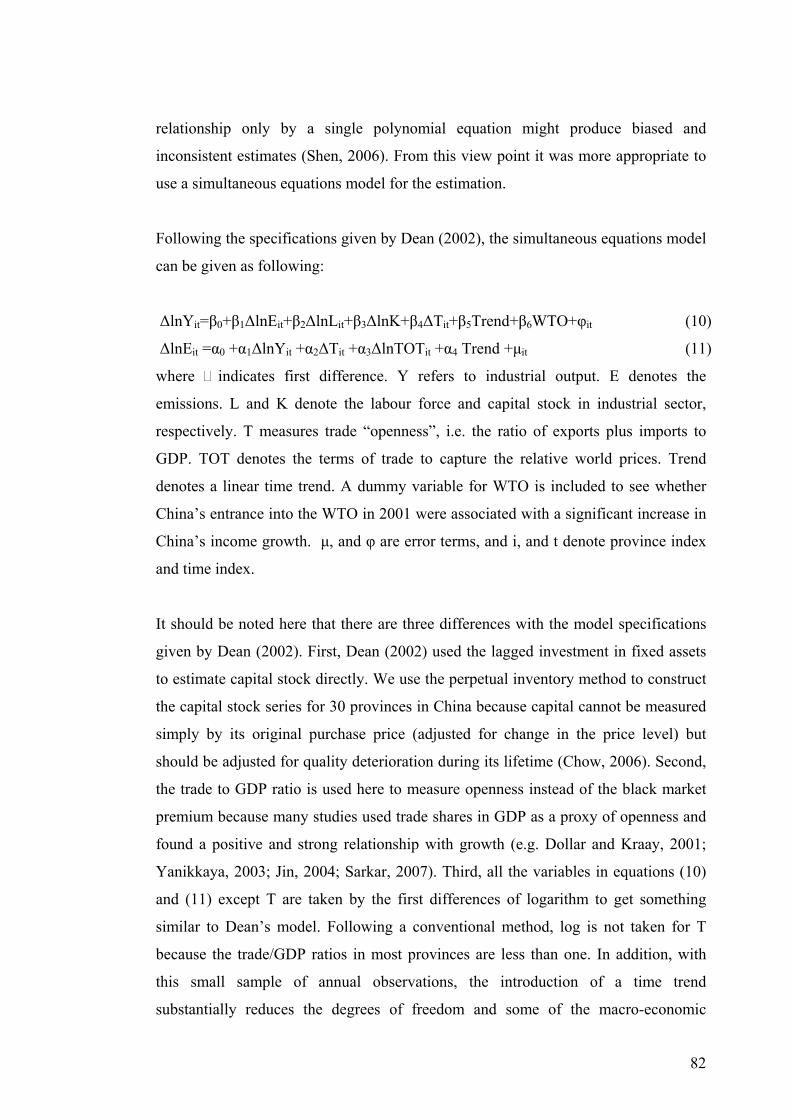
82
relationship only by a single polynomial equation might produce biased and
inconsistent estimates (Shen, 2006). From this view point it was more appropriate to
use a simultaneous equations model for the estimation.
Following the specifications given by Dean (2002), the simultaneous equations model
can be given as following:
ΔlnYit=β0+β1ΔlnEit+β2ΔlnLit+β3ΔlnK+β4ΔTit+β5Trend+β6WTO+φit (10)
ΔlnEit =α0 +α1ΔlnYit +α2ΔTit +α3ΔlnTOTit +α4 Trend +μit (11)
where indicates first difference. Y refers to industrial output. E denotes the
emissions. L and K denote the labour force and capital stock in industrial sector,
respectively. T measures trade “openness”, i.e. the ratio of exports plus imports to
GDP. TOT denotes the terms of trade to capture the relative world prices. Trend
denotes a linear time trend. A dummy variable for WTO is included to see whether
China’s entrance into the WTO in 2001 were associated with a significant increase in
China’s income growth. μ, and φ are error terms, and i, and t denote province index
and time index.
It should be noted here that there are three differences with the model specifications
given by Dean (2002). First, Dean (2002) used the lagged investment in fixed assets
to estimate capital stock directly. We use the perpetual inventory method to construct
the capital stock series for 30 provinces in China because capital cannot be measured
simply by its original purchase price (adjusted for change in the price level) but
should be adjusted for quality deterioration during its lifetime (Chow, 2006). Second,
the trade to GDP ratio is used here to measure openness instead of the black market
premium because many studies used trade shares in GDP as a proxy of openness and
found a positive and strong relationship with growth (e.g. Dollar and Kraay, 2001;
Yanikkaya, 2003; Jin, 2004; Sarkar, 2007). Third, all the variables in equations (10)
and (11) except T are taken by the first differences of logarithm to get something
similar to Dean’s model. Following a conventional method, log is not taken for T
because the trade/GDP ratios in most provinces are less than one. In addition, with
this small sample of annual observations, the introduction of a time trend
substantially reduces the degrees of freedom and some of the macro-economic
83
explanatory variables in the models may be non-stationary. Therefore, the first-
difference form which addresses all these concerns is adopted to estimate the models.
In addition, Dean (2002) only examined water pollution from 1987 to 1995. However,
there were many of important environmental regulations25 in place which internalize
environmental externalities, and some significant trade reforms (e.g. foreign exchange
reforms and entrance into the WTO) undertaken after the middle of 1990s. This
would have impacted on emissions, not only in the water but also the air. Therefore,
this chapter investigates air and water pollution (four key pollutants) during the
period 1990 to 2007.
Following the theoretical implications, Table 5.2 lists the expected signs of all the
explanatory variables in equations (10), and (11). Equation (10) is an income growth
equation. In the production function, output(Y) is a function of capital (K), labour (L),
pollution emission (E), and trade “openness” (T). Both signs of capital change (ΔlnK)
and labour change (ΔlnL) are expected to be positive because the more factors that
are placed in production, the more output is expected. Furthermore, pollution
emissions growth (ΔlnE) is also expected to contribute positively to production.
Because emission (or use of the environment) is treated as an input the total amount
of Y is positively related to the emissions at any point in time. Meanwhile, the ratio
of trade to GDP change (ΔT) is expected to have a positive sign because an increase
in openness will raise the factor productivity and thereby income.
Equation (11) is an emissions growth equation. The sign of the income growth (ΔlnY)
is expected to be either positive or negative. The variable of income growth (ΔlnY) is
applied here to capture the scale and technique effects. More output requires more
factor inputs which results in more pollution (scale effect), while as incomes rise,
people increase their demands for a clean environment and then impose higher
penalties and shift towards clean production process to reduce emissions (technique
effect). The sign is positive if the scale effect dominates the technique effect, but if
the technique effect outweighs the scale effect, a negative sign is permitted. Because
the price of exports relative to imports is used to capture the influence of comparative
25 The detailed discussions are undertaken in Chapter Four.

84
advantage on emissions growth, it can be broken down into the world terms of trade
and trade openness (using ratio of trade to GDP as a proxy). The world terms of trade
change (ΔlnTOT) and the ratio of trade to GDP change (ΔT) are expected to enter
with either a positive or negative sign due to China may or may not have a
comparative advantage in pollution-intensive goods (composition effect). The sign is
negative if China has a comparative advantage in the production of less pollution-
intensive industries. Then the composition of its output will become cleaner after
trade liberalisation. If China has a comparative advantage in pollution-intensive
industries, trade liberalisation may result China specialising in them. Therefore,
positive signs are also permitted. Finally, a time trend is added into both equations to
control the time effect on the dependent variables.
Table 5.2: Expected Signs for the Estimated Coefficients in Eqs. (10), and (11) Equation (10) Equation (11) Explanatory variables Signs Explanatory variables Signs Δln(E) + Δln(Y) +/- Δln(L) + Δln(TOT) +/- Δln(K) + Δ(T) +/- Δ(T) + Source: Author’s compiled from Dean, 2002; Shen, 2008.
5.4.2 Data Description
The sample composes 30 provinces, municipality, and autonomous regions over a
period from 1990-2007. Chongqing is excluded from the sample because in 1996 it
became a municipality directly under the jurisdiction of the central government. In
order to be consistent the relevant data for Chongqing are added to those for the
province of Sichuan. The relationship between four emissions of industrial pollutants
and trade liberalisation based on available data are tested in this chapter. There are
three air pollutants (SO2, Dust, and Smoke) and one water pollutant (COD). The
sources of data are the China Statistical Yearbook (1990-2007) and the China
Environmental Statistical Yearbook (1990-2007).
Because the most complete emissions data available are industrial air and water
pollution emissions, they are used here to represent pollution damage. Emissions are
measured in tons of SO2, Dust, Smoke, and COD. This chapter focuses on Chinese
industry, including mining, manufacturing, and utilities.

85
Income (Y) is measured as the value of industrial output at the provincial level. To
obtain inflation-adjusted data for output value, we deflate the nominal output value
using an index based on a survey of ex-factory prices for industrial output, which is
undertaken by China’s Statistical Bureau since 1984.
The traditional factors of production included in the model are the labour force and
physical capital stock. The labour force is measured by the number of staff and works
on the industrial sector at the year-end.
China’s official statistics do not report estimates of capital stock which would satisfy
international accounting standards. In this chapter fixed capital stock in constant 1990
prices is used as the measure for capital. The capital stock is computed following the
perpetual inventory method (PIM) introduced by Goldsmith (1951). The PIM consist
of adding the net investment data of the current year to an assumed base year of
capital stock. Based on a geometric diminishing model of relative efficiency, the
capital stock for each province can be computed following equation (12):
Kt= Kt-1 (1-δ) + It (12)
where K is capital stock, I is net investment, δ is the depreciation rate and t denotes
time. The calculation takes the following steps (1) use the deflator to obtain a fixed-
asset investment series in constant 1990 prices. For the statistical data in China, there
are two kinds of data series which can be used in the PIM (investment in fixed assts
and the gross fixed capital formation). There is only investment in fixed assets
available for the provincial level so the investment in fixed assets is used to estimate
provincial capital stock in this chapter. Under Standardised National Accounting Xu
(2002) explained that the value of investment in fixed assets at constant prices is
actually calculated using the “price index of fixed asset investment”. The provincial
level data of price index of fixed asset investment are available from various issues of
the China Statistical Yearbook. (2) The base year (1990) initial capital stock for each
province originated from Zhang (2008). (3) As long as a fixed asset ages, both its
efficiency and price go down. Following Perkins (1998), Wang and Fan (2000),
Wang and Yao (2001), and Guo et al. (2006), we adopt 5% as the rate of capital
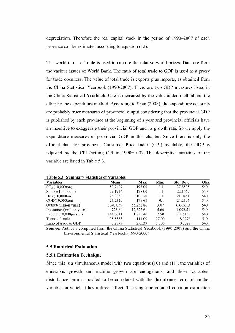
86
depreciation. Therefore the real capital stock in the period of 1990–2007 of each
province can be estimated according to equation (12).
The world terms of trade is used to capture the relative world prices. Data are from
the various issues of World Bank. The ratio of total trade to GDP is used as a proxy
for trade openness. The value of total trade is exports plus imports, as obtained from
the China Statistical Yearbook (1990-2007). There are two GDP measures listed in
the China Statistical Yearbook. One is measured by the value-added method and the
other by the expenditure method. According to Shen (2008), the expenditure accounts
are probably truer measures of provincial output considering that the provincial GDP
is published by each province at the beginning of a year and provincial officials have
an incentive to exaggerate their provincial GDP and its growth rate. So we apply the
expenditure measures of provincial GDP in this chapter. Since there is only the
official data for provincial Consumer Price Index (CPI) available, the GDP is
adjusted by the CPI (setting CPI in 1990=100). The descriptive statistics of the
variable are listed in Table 5.3.
Table 5.3: Summary Statistics of Variables Variables Mean Max. Min. Std. Dev. Obs.SO2 (10,000ton) 50.7407 193.00 0.1 37.8595 540 Smoke(10,000ton) 29.1914 128.00 0.1 22.1667 540 Dust(10,000ton) 25.8338 100.70 0.1 21.0461 540 COD(10,000ton) 25.2529 176.68 0.1 24.2596 540 Output(million yuan) 3740.039 55,252.86 3.07 6,665.13 540 Investment(million yuan) 726.84 12,327.61 5.66 1,002.51 540 Labour (10,000person) 444.6611 1,830.40 2.50 371.5150 540 Terms of trade 98.8333 111.00 77.00 8.7275 540 Ratio of trade to GDP 0.2879 2.0539 0.006 0.3529 540 Source: Author’s computed from the China Statistical Yearbook (1990-2007) and the China
Environmental Statistical Yearbook (1990-2007)
5.5 Empirical Estimation
5.5.1 Estimation Technique
Since this is a simultaneous model with two equations (10) and (11), the variables of
emissions growth and income growth are endogenous, and those variables’
disturbance term is posited to be correlated with the disturbance term of another
variable on which it has a direct effect. The single polynomial equation estimation
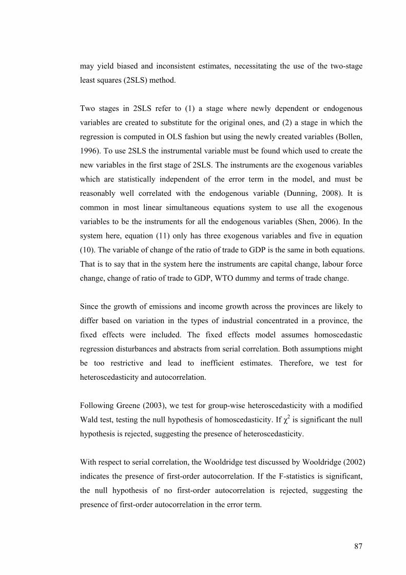
87
may yield biased and inconsistent estimates, necessitating the use of the two-stage
least squares (2SLS) method.
Two stages in 2SLS refer to (1) a stage where newly dependent or endogenous
variables are created to substitute for the original ones, and (2) a stage in which the
regression is computed in OLS fashion but using the newly created variables (Bollen,
1996). To use 2SLS the instrumental variable must be found which used to create the
new variables in the first stage of 2SLS. The instruments are the exogenous variables
which are statistically independent of the error term in the model, and must be
reasonably well correlated with the endogenous variable (Dunning, 2008). It is
common in most linear simultaneous equations system to use all the exogenous
variables to be the instruments for all the endogenous variables (Shen, 2006). In the
system here, equation (11) only has three exogenous variables and five in equation
(10). The variable of change of the ratio of trade to GDP is the same in both equations.
That is to say that in the system here the instruments are capital change, labour force
change, change of ratio of trade to GDP, WTO dummy and terms of trade change.
Since the growth of emissions and income growth across the provinces are likely to
differ based on variation in the types of industrial concentrated in a province, the
fixed effects were included. The fixed effects model assumes homoscedastic
regression disturbances and abstracts from serial correlation. Both assumptions might
be too restrictive and lead to inefficient estimates. Therefore, we test for
heteroscedasticity and autocorrelation.
Following Greene (2003), we test for group-wise heteroscedasticity with a modified
Wald test, testing the null hypothesis of homoscedasticity. If χ2 is significant the null
hypothesis is rejected, suggesting the presence of heteroscedasticity.
With respect to serial correlation, the Wooldridge test discussed by Wooldridge (2002)
indicates the presence of first-order autocorrelation. If the F-statistics is significant,
the null hypothesis of no first-order autocorrelation is rejected, suggesting the
presence of first-order autocorrelation in the error term.

88
In the previous chapter, we found that the inverted-U or N shaped curves held for
most environmental indicators, with the turning point in terms of per capita GDP
around 6,500 yuan (index 1990) in China. Therefore, in this chapter the model is
estimated for three different data sets, one for the whole sample and another for the
divided sub-samples (per capita GDP below 6500 yuan, and above 6500 yuan). The
Chow test is applied to check whether there is any statistically significant difference
in the coefficients obtained from the two sub-samples based on above and below
6,500 yuan. The null hypothesis formulated to check the structural stability of the
emissions change function and income change function is as follows:
H0: Parameters are identical between the sub-samples
H1: Parameters are not identical between the sub-samples
If the F-statistics (calculated using the sum of squared error of the total sample and
sub-samples) is significant, the null hypothesis that the set of coefficients in per
capita GDP below 6,500 yuan equation is equal to the set of coefficients in per capita
GDP above 6,500 yuan equation is rejected.
5.5.2 Results of Estimation
Prior to estimation of the model, the correlation coefficients of independent variables
are examined. Table 5.4 shows that the correlation coefficients are relatively low in
log differences and hence multicollinearity problems may not arise. First differencing
is also widely used as a remedial measure for the multicollinearity problem. If the
variables are highly correlated in levels, the first differences often reduce the
correlation of the variables26.
26 In fact, high correlation was observed when variables were measured in levels.
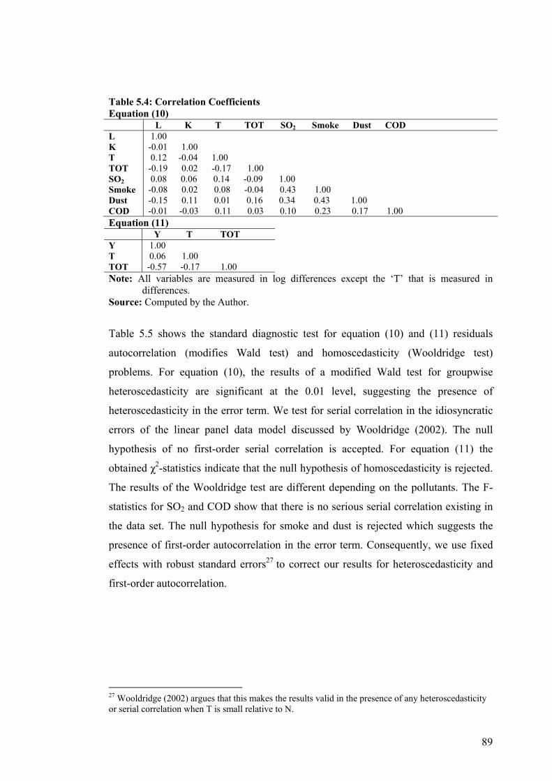
89
Table 5.4: Correlation Coefficients Equation (10) L K T TOT SO2 Smoke Dust COD L K T TOT SO2 Smoke Dust COD
1.00 -0.01 1.00 0.12 -0.04 1.00 -0.19 0.02 -0.17 1.00 0.08 0.06 0.14 -0.09 1.00 -0.08 0.02 0.08 -0.04 0.43 1.00 -0.15 0.11 0.01 0.16 0.34 0.43 1.00 -0.01 -0.03 0.11 0.03 0.10 0.23 0.17 1.00
Equation (11) Y T TOT Y T TOT
1.00 0.06 1.00 -0.57 -0.17 1.00
Note: All variables are measured in log differences except the ‘T’ that is measured in differences.
Source: Computed by the Author.
Table 5.5 shows the standard diagnostic test for equation (10) and (11) residuals
autocorrelation (modifies Wald test) and homoscedasticity (Wooldridge test)
problems. For equation (10), the results of a modified Wald test for groupwise
heteroscedasticity are significant at the 0.01 level, suggesting the presence of
heteroscedasticity in the error term. We test for serial correlation in the idiosyncratic
errors of the linear panel data model discussed by Wooldridge (2002). The null
hypothesis of no first-order serial correlation is accepted. For equation (11) the
obtained χ2-statistics indicate that the null hypothesis of homoscedasticity is rejected.
The results of the Wooldridge test are different depending on the pollutants. The F-
statistics for SO2 and COD show that there is no serious serial correlation existing in
the data set. The null hypothesis for smoke and dust is rejected which suggests the
presence of first-order autocorrelation in the error term. Consequently, we use fixed
effects with robust standard errors27 to correct our results for heteroscedasticity and
first-order autocorrelation.
27 Wooldridge (2002) argues that this makes the results valid in the presence of any heteroscedasticity or serial correlation when T is small relative to N.
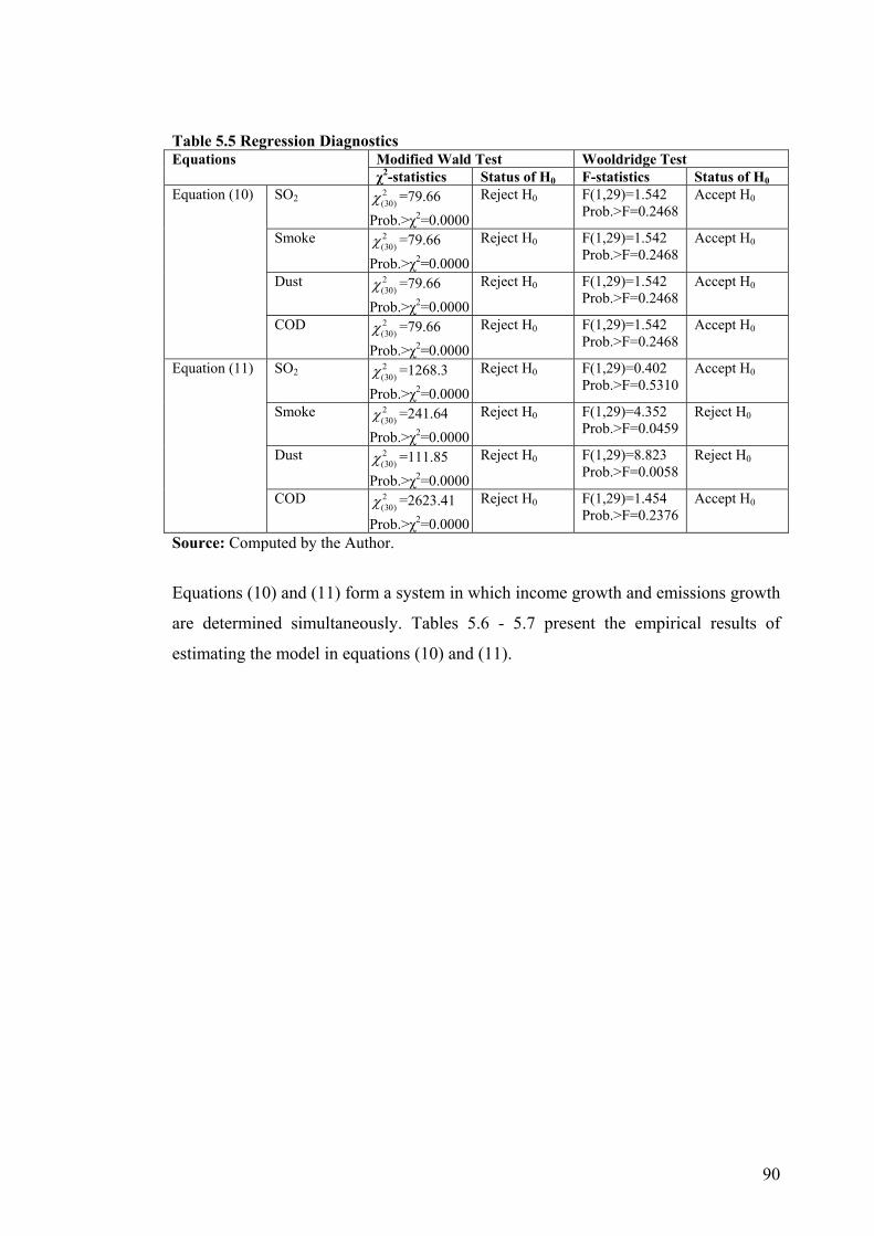
90
Table 5.5 Regression Diagnostics Modified Wald Test Wooldridge Test Equations χ2-statistics Status of H0 F-statistics Status of H0
SO2 2(30)χ =79.66
Prob.>χ2=0.0000
Reject H0 F(1,29)=1.542 Prob.>F=0.2468
Accept H0
Smoke 2(30)χ =79.66
Prob.>χ2=0.0000
Reject H0 F(1,29)=1.542 Prob.>F=0.2468
Accept H0
Dust 2(30)χ =79.66
Prob.>χ2=0.0000
Reject H0 F(1,29)=1.542 Prob.>F=0.2468
Accept H0
Equation (10)
COD 2(30)χ =79.66
Prob.>χ2=0.0000
Reject H0 F(1,29)=1.542 Prob.>F=0.2468
Accept H0
SO2 2(30)χ =1268.3
Prob.>χ2=0.0000
Reject H0 F(1,29)=0.402 Prob.>F=0.5310
Accept H0
Smoke 2(30)χ =241.64
Prob.>χ2=0.0000
Reject H0 F(1,29)=4.352 Prob.>F=0.0459
Reject H0
Dust 2(30)χ =111.85
Prob.>χ2=0.0000
Reject H0 F(1,29)=8.823 Prob.>F=0.0058
Reject H0
Equation (11)
COD 2(30)χ =2623.41
Prob.>χ2=0.0000
Reject H0 F(1,29)=1.454 Prob.>F=0.2376
Accept H0
Source: Computed by the Author.
Equations (10) and (11) form a system in which income growth and emissions growth
are determined simultaneously. Tables 5.6 - 5.7 present the empirical results of
estimating the model in equations (10) and (11).

91
Table 5.6: Estimated Results for Equation (11) ΔlnEit =α0 +α1ΔlnYit +α2ΔTit +α3ΔlnTOTit +α4 Trend +μit
SO2 Smoke Dust COD Full
sample <
6,500 >
6,500 Full
sample <
6,500 >
6,500 Full
sample <
6,500 >
6,500 Full
sample <
6,500 >
6,500 Cons. -0.173**
(-2.69) -0.24 (-1.55)
-0.24*
(-1.79) 0.126 (1.33)
0.20 (0.92)
-0.31 (-1.55)
0.050 (0.41)
-0.57*
(-1.86) -0.60**
(-2.59) -0.23***
(-3.45) 0.03 (0.20)
-0.42***
(-2.93) ΔlnY 1.21**
(2.36) 0.09 (0.79)
-0.25***
(-2.69) -1.70**
(-2.26) 0.12 (0.77)
-0.20*
(-1.67) -0.71*
(-1.66) -0.01 (-0.04)
0.11
(0.69) 1.34**
(2.57) 0.06 (0.54)
-0.27***
(-2.69) ΔlnTOT 2.57**
(2.25) 4.43 (1.24)
7.95**
(2.44) -3.48**
(-2.07) -7.55 (-1.48)
8.78*
(1.79) -0.33*
(-1.78) 13.4*
(1.87) 18.86***
(3.33) 3.22***
(2.76) -0.72 (-0.21)
9.17***
(2.63) ΔT 0.005
(0.05) -0.06 (-0.23)
0.28*
(1.88) -0.006 (-0.04)
-0.28 (-0.71)
0.49**
(2.18) 0.035 (0.21)
0.51 (0.91)
0.72***
(2.77) 0.21**
(2.29) 0.22 (0.81)
0.43***
(2.70) Time Trend
0.004**
(2.19) 0.003 (0.42)
-0.02***
(-2.88) 0.005 (1.61)
0.03***
(3.11) -0.04***
(-2.97) 0.005 (1.29)
0.0002 (1.58)
-0.05***
(-3.47) 0.001 (0.64)
-0.0003 (-0.05)
-0.02*
(-1.90) R2 0.034 0.039 0.072 0.017 0.052 0.061 0.027 0.050 0.072 0.020 0.035 0.068 F-test 4.15*** 1.85 3.29*** 2.04* 2.50** 2.75** 3.31** 2.43** 3.28*** 2.44** 1.69 3.06**
Obs. 510 264 246 510 264 246 510 264 246 510 264 246 Notes: 1. ΔlnY=income growth; ΔlnTOT=world terms of trade; ΔT=the ratio of trade to GDP change; all variables are measured in log differences except Time Trend, and T that is measured in differences; 2. t-statistics in parentheses; ***Significant at the 1% level; **significant at the 5% level; *significant at the 10% level; 3. Includes fixed effects for provinces. Standard errors corrected for group-wise heteroscedasticity and first-order autocorrelation.

92
Table 5.7: Estimated Results for Equation (10) ΔlnYit=β0+β1ΔlnEit+β2ΔlnLit+β3ΔlnK+β4ΔTit+β5Trend+β6WTO+φit
Y Y Y Y Full
sample <
6,500 >
6,500 Full
sample <
6,500 >
6,500 Full
sample <
6,500 >
6,500 Full
sample <
6,500 >
6,500 ΔlnSO2 -17.16***
(-10.02) 2.23***
(7.24) 2.55***
(5.55)
ΔlnSmoke 19.42***
(10.02) 0.88***
(7.24) 1.00***
(5.55)
ΔlnDust -1.42***
(-10.02) 10.67***
(7.24) 12.21***
(5.55)
ΔlnCOD -5.21***
(-10.02) 263.9***
(7.24) 302.1***
(5.55) Cons. 0.01
(0.50) -0.36***
(-5.40) 0.48***
(5.23) 1.84***
(10.42) -0.03 (-1.20)
0.10**
(2.33) 0.18***
(9.75) 2.99***
(6.99) 3.49***
(5.58) 0.04**
(2.18) 8.25***
(7.15) 9.51***
(5.56) ΔlnL 1.41***
(10.21) 0.30***
(3.69) 0.33**
(2.32) 4.63***
(10.34) 0.26***
(3.24) 0.28**
(2.01) -0.77***
(-6.66) 6.62***
(7.32) 7.56***
(5.57) 0.56***
(5.64) 31.66***
(7.26) 36.2***
(5.56) ΔlnK 0.09***
(9.11) 0.01**
(2.46) 0.02***
(3.28) -0.06***
(-8.89) 0.01***
(2.73) -0.01 (-0.85)
0.03***
(6.56) -0.11***
(-7.24) -0.11 (-0.40)
0.03***
(5.89) -0.81***
(-7.28) 0.92***
(5.55) ΔT 1.72***
(9.63) 0.04 (0.26)
0.11***
(5.40) 2.68***
(9.89) -0.20 (-1.36)
0.15**
(2.17) 0.06***
(6.52) -0.04 (-0.27)
0.03***
(4.87) 0.53***
(6.68) 16.9***
(7.24) 19.2***
(5.56) Time Trend 0.01***
(4.52) 0.05***
(7.01) 0.06***
(6.70) 0.15***
(9.61) 0.02***
(5.78) 0.03***
(6.30) 0.008***
(3.37) 0.40***
(7.26) 0.47***
(5.75) 0.03***
(7.71) 3.43***
(7.24) 3.93***
(5.57) WTO Dummy 1.09***
(10.42) -0.37***
(-5.78) 0.44***
(5.08) 1.16***
(10.41) 0.09**
(2.56) 0.13***
(3.10) 0.16***
(6.93) 2.93***
(7.14) 3.37***
(5.54) 0.55***
(10.41) 37.5***
(7.23) 42.9***
(5.55) R2 0.33 0.20 0.28 0.32 0.20 0.28 0.326 0.20 0.28 0.326 0.20 0.28
F-test 38.22*** 9.79*** 13.63*** 38.22*** 9.79*** 13.63*** 38.22*** 9.79*** 13.63*** 38.22*** 9.79*** 13.63***
Obs. 510 264 246 510 264 246 510 264 246 510 264 246
Notes: 1. ΔlnE=emissions growth (SO2, smoke, dust, and COD); ΔlnL=labour change; ΔlnK=capital change; ΔT=the ratio of trade to GDP change; all variables are measured in log differences except Time Trend, WTO Dummy, and T that is measured in differences;
2. t-statistics in parentheses; ***Significant at the 1% level; **significant at the 5% level; *significant at the 10% level; 3.Includes fixed effects for provinces. Standard errors corrected for group-wise heteroscedasticity and first-order autocorrelation.

93
5.5.2.1 Full sample
First, trade liberalisation will directly affect emissions growth via its effect on the
relative price of pollution-intensive goods. Two variables are assigned to capture this
effect, TOT and the trade to GDP ratio.
the world terms of trade (TOT) show a strong positive relationship with the growth of
emissions for air pollutant SO2 emissions growth and water pollutant COD emissions
growth (see Table 5.6 for equation 11). A 1% increase in the TOT causes SO2 growth
to rise by 2.57%, while a 1% increase in the TOT leads to an increase in the growth
of COD emissions of 3.22%. At the same time a 1% increase in trade openness (T)
raises the COD emissions growth by 0.21%. This result confirms the pollution haven
hypothesis and suggests that China may have a comparative advantage in SO2 and
COD pollution-intensive goods.
Unlike the SO2, and COD emissions, for air pollutant smoke emissions, a 1% large
increase in the TOT reduces the smoke growth by 3.48%. However, for air pollutant
dust emissions, a 1% increase in the TOT causes the dust growth to decline by 0.33%.
This negative relationship shows that China may have a comparative disadvantage in
the smoke and dust pollution-intensive goods.
Therefore, the direct composition effect of trade liberalisation impacted badly on
China’s water environment (COD emissions) and SO2 emissions problem but is good
for smoke and dust emissions problem.
Second, trade liberalisation will affect emissions growth indirectly via its effect on
income growth (scale effect increases emissions while technique effect decreases
emissions). This indirect impact measured by the coefficient of the ratio of trade to
GDP in equation (10) (see Table 5.7) multiplying the coefficient of the income
growth in equation (11) (see Table 5.6).
The indirect impact via income growth for SO2 shows that a 1% increase in openness
(T) produces an increase of 1.72% in income growth (Y), and a 1% increase in Y
increases SO2 growth by 1.21% and therefore an increase of 2.08% (=1.72*1.21) of

94
SO2 growth. For COD, a 1% rising in growth of T leads to increased Y by 0.53%.
And this increase in Y, via freer trade, causes COD emission going up by 0.71%
(=1.34*0.53). Since the variable of income growth refers to a combination of scale
and technique effects in equation (11), the SO2 and COD emissions increase with a
rise in income at an increasing rate suggests that the scale effect dominates the
technique effect for SO2 and COD. Hence, the indirect income effect of trade
liberalisation may indeed be a worsening of the SO2 and COD pollution problem.
The technique effect outweighs the scale effect for smoke and dust emissions growth,
which means that increased income due to increased trade can reduce industrial
smoke and dust emissions growth. For example, for smoke emissions, a 1% rise in the
T leads to an increase of 2.68% in the Y and then a 2.68% increase in income growth
causes a reduction in smoke emissions by -4.56% (=-1.70*2.68); and for dust
emissions, a 1% increase in openness can raise the growth of income by 0.06%, and
then reduce the dust emission growth by -0.04% (=-0.71*0.06). This negative
relationship between income growth and smoke and dust emissions growth would
reflect the technique effect of trade liberalisation. As incomes rise people increase
their demands for a clean environment and then industrial firms have an incentive to
shift towards cleaner production processes to reduce emissions. So the indirect
income effect of trade liberalisation on the environment is to reduce the problem of
smoke and dust pollution.
Turning to the estimated results of the income growth equation (see Table 5.7 for
equation 10), most of the estimated coefficients are highly significant and consistent
with the expected signs. The traditional factors such as labour force growth and
physical capital growth contribute positively to the industrial output growth (except
the capital growth for smoke). The emissions growths of SO2, dust and COD have a
negative influence on the income growth which might be due to the differing
concentrations of pollution-intensive industries across the provinces. In addition,
China’s entrance into the WTO in 2001 seems to have been associated with a
significant increase in the growth of income.

95
5.5.2.2 Sub-Samples
The Chow test is used to establish whether there is any statistically significant
difference in the coefficients obtained for the two sub-samples, based on the per
capita GDP above and below 6,500 yuan. Table 5.8 represents the results of the Chow
structural stability test. All the F-statistics obtained in the emissions growth equation
and income growth equation are greater compared to the 10% critical value of the
statistics. Therefore, the null hypothesis that there is no difference between the sub-
samples is rejected. The result clearly indicates that there is a significant difference
between the two sub-samples.
Table 5.8: Chow Test Results Equations F-Critical Value F-Statistics Status of H0
SO2 F=1.96 Reject H0 Smoke F=1.89 Reject H0 Dust F=1.75 Reject H0
Equ. (10)
COD
F(7,496)=2.64 at 1% level F(7,496)=2.01 at 5% level
F(7,496)=1.72 at 10% level F=2.01 Reject H0
SO2 F=3.01 Reject H0 Smoke F=3.83 Reject H0 Dust F=2.31 Reject H0
Equ. (11)
COD
F(5,500)=3.02 at 1% level F(5,500)=2.21 at 5% level
F(5,500)=1.85 at 10% level F=2.31 Reject H0
Source: Computed by the Author.
Regressions are run on two sub-samples, one with the sample of per capita GDP
below 6,500 yuan and the other with the sample of per capita GDP above 6,500 yuan.
The structural stability test of the coefficients gives us new results utilising both sub-
samples for all the pollutants (see Table 5.6 and 5.7). We focus on the sample of per
capita GDP below 6,500 yuan because most of the variables are statistically
significant in both equations for most of pollutants (SO2, smoke and COD). Sub-
samples based on above 6,500 yuan per capita income yield the most significant
difference. As expected the provinces with a higher income give a better overall fit
than those with lower incomes. The R2 improves compared with the full sample. The
expected signs are similar for the full sample except the income in SO2, and COD
(equation 10) and the coefficients are stronger than the full sample.
The direct composition effect of trade liberalisation for all pollutants impacts badly
because the terms of trade (TOT) and openness (T) show strong positive relationships
with the growth of emissions. Table 5.6 shows that an increase in the relative price of

96
net exports leads to all the emissions growth rising while increased openness cause an
increase in growth of emissions. These results suggest that China may have a static
comparative advantage in pollution-intensive goods. Hence, the direct impact of trade
liberalisation on the composition of output may indeed lead to a worsening of the
pollution problem at the high income level stage.
At the same time the indirect impact via income growth shows an increase in income
due to increased trade reduces all the emissions growth. Table 5.7 presents that
increase trade openness produces an increase in income growth, while turning to
Table 5.6 we find that an increase in the income growth causes a reduction in all
emissions growth. These negative results indicate that the technique effect outweighs
the scale effect. As income rises to a critical level, in this study say 6,500 yuan,
people increase their demands for clean environment which then restrict industry’s
ability to pollute the air and water. Therefore, the indirect role of trade liberalisation,
via its effect on income growth, is to reduce the pollution problem.
5.5.2.3 The Net Trade Liberalisation Impact
The 2SLS method provides a way to investigate the impact trade liberalisation on the
environment by two sources, the direct impact measured by the coefficient of trade
openness (ΔT) in equation (11), and indirect impact measured by the coefficient of
openness (ΔT) in equation (10) multiplying the coefficient of income growth (ΔlnY)
in equation (11), therefore the net impact should be calculated as the net values of
these two impact.
Table 5.9 presents the net trade liberalisation impact on emissions of pollutants. For
the full sample we only focus on the COD because the variable of trade openness for
other pollutants in Equ. (11) is not significant. The net impact is that a 1% increase in
international trade causes a net increase of 0.24% (=direct impact 0.21% + indirect
impact 0.03%) in COD growth. However, where the sub-sample that per capita GDP
is above 6,500 yuan, the results show that there is indeed both a direct and indirect
effect of trade liberalisation on emissions growth and these effects are of opposite
signs. Improvements in the openness of trade lead to increased emissions growth.
Therefore, the direct impact of trade liberalisation would be to aggravate

97
environmental damage. However, the results also indicate that increase openness
significantly raises the income growth which has a negative and significant effect on
the emissions growth. Hence the indirect impact of trade liberalisation is to mitigate
any environmental damage. Combining the direct and indirect impacts, we can see
the different net impact of trade liberalisation on air and water environments. For air
pollutants SO2 and smoke, although a negative indirect impact emerges, the positive
direct impact is greater than the negative direct impact. This evidence indicates that
increases in trade openness will increase emissions but slow the growth. The
technique effect dominates the scale effect and the positive composition effect for
water pollutant COD. This negative net impact indicates that trade reduces water
pollutant emissions in China.
Table 5.9: The Net Trade Liberalisation Impact on Pollutants Emissions Pollutants Direct impact Indirect impact Net impact
Full sample COD +0.21 (+1.34*0.53)=+0.71 +0.92 SO2 +0.28 (-0.25*0.11)= -0.03 +0.25
Smoke +0.49 (-0.20*0.15)= -0.03 +0.46 Sub-sample
> 6,500 COD +0.43 (-0.27*19.2)= -5.18 -4.75
Note: 1. Direct impact measured by the coefficient of ΔT in Equ. (11), from Table 5.6; 2. Indirect impact measured by the coefficient of income growth in Equ. (11), from
Table 5.5, multiplying the coefficient of openness in Equ. (10), from Table 5.7; 3. Net impact equals to direct impact plus indirect impact.
5.6 Conclusion
This chapter uses the Chinese provincial data from 1990 to 2007 to estimate a
modified version of Dean (2002) model. The empirical analysis provides several
conclusions. First, the scale effect for air pollutant (SO2) and water pollutant (COD)
outweigh the technique effect, whilst the technique effect dominates the scale effect
for air pollutants (smoke and dust). Second, the composition effect for SO2 and COD
emissions are estimated to be significantly positive on emissions growth, but negative
on the growth of smoke and dust emissions. Third, the results indicate that China may
have a comparative advantage on SO2 and COD pollution-intensive goods, but on less
smoke and dust pollution-intensive goods. Therefore, Chinese experience shows that
trade liberalisation does not necessarily result in a developing country specialising in
pollution-intensive industry, and for some primary pollutants, the scale effect of trade
liberalisation offset other environmental gains from specialisation and increased
access to international best practice in pollution control.

98
Furthermore, in order to test the hypothesis that higher income has a greater impact
on the activities that motivate cleaner environment, this simultaneous system is
estimated by splitting the full sample into activities with above and below 6,500 yuan
per capita GDP level. We found a significant difference in the sub-samples. Sub-
sample based on above 6,500 yuan yield the most significant difference for SO2,
smoke, and COD activities. At the provincial level rising income per capita is
associated with rising direct impact and falling indirect impact for SO2, smoke, and
COD, so that higher per capita income provinces tend to show relatively better
technique effect in emissions. For COD, indirect impact is higher than direct impact,
generating negative net impact and revealing overall reduction in emissions, which is
consistent with those found by Dean (2002), Chai (2002), and Shen (2008).
The next chapter will be devoted to the summary and policy recommendations that
can be drawn from this study.

99
CHAPTER SIX
SUMMARY AND RECOMMENDATIONS
6.1 Summary
Since the late 1970s and early 1980s, China has experienced monumental historical
changes. The economic reforms began with a shift from farming work to a system of
household responsibility to phase out collectivised agriculture. This later expanded to
include the gradual liberalisation of prices; fiscal decentralisation, and increasing
autonomy for state enterprises that gave local government officials and plant
managers more authority. In turn, this resulted in a wider variety of private enterprise
in services and light manufacturing, a diversified banking system, the development of
stock markets, a rapid growth in the non-state sector, and an economy more open to
increased foreign trade and investment. As its role in world trade has steadily grown,
China’s importance to the international economy has also increased apace. The
government has focused on foreign trade as a major vehicle for economic growth.
China’s GDP has increased tenfold since 1978, largely due to economic reforms
including the liberalisation of its economy.28 The per capita income has grown at an
average annual rate of more than 8% over the last three decades, drastically reducing
poverty, and China’s foreign trade has grown faster than its GDP for the past 25 years
(Chen and Li, 2000).
With this rapid growth in foreign trade and the economy since the 1980s, China’s
environment in absolute terms of pollutants emissions, has become more severely
polluted in recent years. Two-thirds of the 338 cities for which air quality data are
available are polluted moderately or severely. Ninety percent of urban water bodies
are severely polluted. Although China has passed environmental legislation and
participated in some international anti-pollution conventions, pollution will continue
be a serious problem for years to come. However, in per capita term of emissions
there is a declining trend of industrial pollution despite having the largest and
increasing fast growing population. For example, per capita emissions of SO2 first
increased from 1990 to a peak in 1997 but began to drop slowly from 1998 before
28 CIA, The World Factbook, 2009.

100
rising again after 2002. The per capita emissions of COD, smoke and dust showed a
slow but significant decline during the same period (see Figure 6.1).
Figure 6.1: Per capita emissions in China, 1990-2007
0
0.005
0.01
0.015
0.02
1990 1991 1992 1993 1994 1995 1996 1997 1998 1999 2000 2001 2002 2003 2004 2005 2006 2007
so2 cod smoke dust
Source: Author’s calculation based on data from the China Statistical Yearbook, and the China Environmental Yearbook, various issues.
Due to these facts several researchers were interested in studying the relationship
between trade, economic growth, and the environment over recent years.
Unfortunately their empirical results are mixed and therefore disentangling this issue
is important and the research of this thesis is necessary. Majority of the studies are
based on the single equation where there is no feedback from pollution to trade
liberalisation. Therefore, our contribution is to use a simultaneous equations model
for the estimation. In addition, we extend this simultaneous model by adding different
variables, and investigate four key pollutants empirically from 1990 to 2007.
The primary purpose of this thesis was to study the nexus of trade, economic growth,
and the environment in China from 1990 to 2007. We hypothesised that (a) the
Environmental Kuznets Curve (EKC) hypothesis. It is possible to capture the
relationship between per capita of income and per capita of pollutants emissions by
using the standard quadratic or cubic EKC models based on cross-country or a single
country. This approach has been used in a number of studies such as Grossman and
Krueger (1991), Selden and Song (1994), and Dinda et al. (2000). Both quadratic and
cubic EKC models were used for this work. (b) Trade liberalisation has a short term
negative effect on the environment but a long term positive effect will occur provided
that externalities can be internalised with the rise in income and new technology. By

101
applying the methodology developed by Dean (2002) and modifying her model, a
simple Heckscher-Ohlin (HO) model with endogenous factor supply has been used
for this study to capture the impact of trade liberalisation on the environment.
The study of the relationship between per capita income and per capita emissions for
the whole country would not provide a complete picture due to unbalanced
development among the regions. Therefore this study took a further step by grouping
the whole country into the developed costal region and the relatively poor central and
western regions. A combination of the results from the whole country and different
regions could explain the linkage between economic growth and environmental
pollution better. Moreover, a study of EKC based on a single country at various
development levels is better than one on cross-country because the source of income
and expenditure pattern varies across countries. Cross-country regression relating
policy variables seem to be sensitive to slight alterations in the policy variables and
small changes in the sample of countries chosen.
A study of the impact of trade liberalisation on the environment from 1990 to 2007
would not reveal a satisfying picture because the economy grew rapidly during this
period, and the income and technique effects might be different at the different
income levels. Hence, the whole sample was split into activities that were above and
below 6,500 yuan per capita GDP levels. The results could be expected to be different
between the whole sample and sub-samples, even among pollutants in the same
sample.
6.2 Major Findings
To determine the relationship between trade liberalisation, economic growth, and the
environment the estimation results from different models, different samples, and
different pollutants can be merged to reveal the whole picture. The EKC hypothesis is
not clear in China because the relationship between environmental quality and
income varies on the types of pollutants and regions. The inverted-U shaped EKC
only holds for per capita SO2 emissions while the N-shaped relationship between per
capita emission and income is also found for smoke, dust and COD in the different
regions.
102
The first major finding is the turning points of EKC for the whole country and
different regions. The turning point for SO2 in terms of per capita GDP occurred
around 6,376 yuan (index 1990) for the whole country, which is consistent with the
estimations of Llorca and Meunie (2009) (3,333-4,596 yuan), and He (2008) (8,392-
10,226 yuan), and is well suited to the actual condition in China. Compared to the
experience of other developed countries China entered this decreasing part of the
EKC at an earlier stage but comparing the estimation results of different regions, the
poor central and western regions appear to have turning points at lower income levels
than the relatively developed coastal region. This suggests that technology diffusion,
leapfrogging, and institutional imitation through learning among regions at different
stages of development may have played an important role in reducing pollution
emissions (Jiang et al., 2008). Based on these results, Jiang et al. recommend that
governments should facilitate advanced technology diffusion and transfer and
encourage knowledge sharing at less developed regions to move forward. Moreover
the concerned government agencies at various levels should be encouraged to share
successful regulatory experiences.
The second major finding is that China may have a comparative advantage on SO2
and COD pollution-intensive goods, but on less smoke and dust pollution-intensive
goods. The composition effects for whole sample are estimated to be significantly
positive on SO2 and COD emissions growth but negative on the growth of smoke and
dust emissions. Therefore the Chinese experience shows that trade liberalisation does
not necessarily result in a developing country specialising in pollution-intensive
industry, and for some primary pollutants the scale effect of trade liberalisation
offsets other environmental gains from specialisation and increased access to
international best practice in pollution control. Furthermore the scale effect for SO2
and COD outweighs the technique effect which is evidence for the pollution haven
hypothesis. This is confirmed for COD which shows that direct and indirect impacts
are positive and resulted in an increase in net emission due to an increase in trade.
In order to obtain further evidences for our hypothesis, the whole sample is split into
the above and below 6,500 yuan turning point income of EKC. The third major

103
finding is that the split sample (above 6,500 yuan per capita income) provides limited
support for the EKC hypothesis, and at the provincial level, rising income per capita
is associated with rising direct impact and falling indirect impact for SO2, smoke, and
COD, so that provinces with higher per capita incomes tend to show relatively better
technique effect in emissions. The indirect impact for COD is higher than the direct
impact which generates a negative net impact that reveals an overall reduction in
emissions, which is consistent with those found by Dean (2002), Chai (2002), and
Shen (2008). This suggests that a rising income via increased international trade is
associated with lowering COD emissions (net impact) and tend to lower the SO2 and
smoke (indirect impact) in China.
6.3 Policy Recommendations
From these results it is clear that trade liberalisation leads to both benefits and costs
on the environment in China. First, the author recommends that the government
embark on further trade liberalisation to promote economic growth and raise incomes.
Liberalisation brings a bundle of management experience, marketing channels, and
technology, which provides a unique opportunity to learn from other countries’
experiences and thereby avoid some of the mistakes. Second, the government should
encourage changing the current trade structures by supporting and raising the
competitiveness of less pollution-intensive industries in the international market
which will push pollution-intensive industries towards clean production and exports.
More importantly, the change of trade structures also needs the support of technology.
The government should promote imports for heavily polluting industries and
encourage the application of advanced foreign technology by granting financial
support and reducing taxes. In addition, strengthening and enforcing environmental
regulations is an effective way to prevent the pollution-intensive industry transferring
to China from other developed countries.
6.4 Limitations and Future Studies
This thesis is limited in several respects. Firstly, to narrow the analysis to manageable
proportions, this paper focuses on the industry sector. Secondly, due to data
constraints, it focuses only on China’s domestic pollution problems. No attempt was
made to look at the problem in a global context. Further investigation of various

104
emissions would provide more information about the economic consequences of links
between trade and the environment. Thirdly, the model does not include a complete
explanation for the growth of emissions in China. The small-country trade model
used here leads to a simple specification in where the price of environmental damage
is determined solely by world markets. Furthermore, the period for our analysis was a
relatively small time frame in which to observe long-term changes in the composition
of industries. This analysis can only capture these influences using fixed effects.
Finally, trade affects the environment via scale, composition, and technique effects,
and these can all be expected to vary across countries. Our work has demonstrated
how these effects can be isolated and estimated. Future work in this area should be
attempting to refine, extend, and improve on these methods.
105
REFERENCES
Antweiler, W., Copeland, B. R., and Taylor, M. S. 2001. “Is Free Trade Good for the Environment?” The American Economic Review, 91: 877-908. Barrett, S., and Graddy, K. 2000. “Freedom, Growth and the Environment.” Environmental and Development Economics, 5: 433-456. Baumol, W., and Oates, W. 1988. “The Theory of Environmental Policy,” Cambridge University Press, New York. Beckerman, W. 1992. “Economic Growth and the Environment: Whose Growth? Whose Environment?” World Development, 20:481-496. Beghin, J., Bowland, B., Dessus, S., Roland-Holst, D., and van der Mensbrugghe, Dominique. 2002. “Trade Integration, Environmental Degradation, and Public Health in Chile: Assessing the Linkages.” Environment and Development Economics, 7:241-267. Beghin, J., Roland-Holst, D., and van de Mensbrugghe, D. 1995. “Trade Liberalization and the Environment in the Pacific Basin: Coordinated Approaches to Mexican Trade and Environment Policy.” American Journal of Agricultural Economics, 77:778-785. Bhagwati, J. 1993. “The Case for Free Trade,” Scientific American, 269:18-23. Blacksmith Institute, 2007. “The World’s Worst Polluted Places: The Top Ten of the Dirty Thirty.” Accessed 12/09/2008, http://www.worstpolluted.org/ Bollen, K. A. 1996. “An Alternative Two Stage Least Squares (2SLS) Estimator for Latent Variable Equations.” Psychometrika, 61:109-121. Borghesi, S. 1999. “The Environmental Curve: A Survey of the Literature,” FEEM Working Paper No. 85-99, accessed 21/10/2008, http://papers.ssrn.com/sol3/papers.cfm?abstract_id=200556 Bradford, D. F., Schlieckert, R., and Shore, S. H. 2000. “The Environmental Kuznets Curve: Exploring a Fresh Specification,” NBER Working Paper No. 8001. Brown, D. K., Deardorff, A. V., and Stern, R. M. 1992. “A North American Free Trade Agreement: Analytical Issue and a Computational Assessment,” World Economy, 15:11-29. Cann, C. W., Cann, M. C., and Gao, S. 2004. “China’s Road to Sustainable Development,” in Day, K.A. (ed.), “China’s Environmental and the Challenge of Sustainable Development,” M.E. Sharpe, pp3-34.

106
CAS (Chinese Academic of Sciences), 2006. “Report on China’s Sustainable Development 2006,” Science Publishing House, Beijing. CIA (Central Intelligence Agency), The World Factbook, China. Accessed 08/05/2009. https://www.cia.gov/library/publications/the-world-factbook/geos/CH.html Chai, C. H. 2002. “Trade and Environment: Evidence from China’s Manufacturing Sector,” Sustainable Development, 10: 25-35. Chan, A. 2001. “Mao’s Crusade: Politics and Policy Implementation in China’s Great Leap Forward,” Oxford University Press, UK. Chen, W. 2007. “Economic Growth and the Environment in China”, in Proceeding of the Annual Conference on Development and Change, Cape Town, 2007, accessed 08/04/2008,http://www.policyinnovations.org/ideas/policy_library/data/01447/_res/id=sa_File1/paper.pdf Chen, B. Z., and Li, F. 2000. “Determinants of Economic Growth in China: Private Enterprise, Education, and Openness.” China Economic Review, 11:1-15. China Environment Yearbook (various issues). Beijing, China: Ministry of Environmental Protection. China Statistical Yearbook (various issues). Beijing, China: National Bureau of Statistics. Chintrakarn, P., and Millimet, D. L. 2006. “The Environmental Consequences of Trade: Evidence from Subnational Trade Flows,” Journal of Environmental Economics and Management, 52: 430-453. Chow, G. C. 2006. “New Capita Estimates for China: Comments.” China Economic Review, 17: 186-192. Chua, S. 1999. “Economic Growth, Liberalization, and the Environment: A Review of the Economic Evidence,” Annual Review of Energy and the Environment, 24:391-430. Cleveland, C.J., Costanza, R., Hall, C.A.S., and Kaufmann, R., 1984. “Energy and the US Economy: a Biophysical Perspective.” Science, 225: 890–897. Cole, M. A. 2004. “Trade, the Pollution Haven Hypothesis and the Environmental Kuznets Curve: Examining the Linkages.” Ecological Economics, 48:71-81. Cole, M. A., and Elliott, R. J. R. 2003. “Determining the Trade-Environment Composition Effect: The Role of Capital, Labour and Environmental Regulations.” Journal of Environmental Economics and Management, 46:363-383.

107
Cole, M. A., and Rayner, A. J. 2000. “The Uruguay Round and Air Pollution: Estimating the Composition, Scale and Technique Effects of Trade Liberalization,” Journal of International Trade and Economic Development, 9: 339-354. Cole, M. A., Rayner, A. J., and Bates, J. M. 1997. “The Environmental Kuznets Curve: An Empirical Analysis.” Environmental and Development Economics, 2: 401-416. Copeland, B. R. and Taylor, M. S. 2004. “Trade, Growth, and the Environment.” Journal of Economic Literature, XLII: 7-71. Daly, H. 1993. “The Perils of Free Trade,” Scientific American, 269:50-57. De Bruyn, S. M. 1998. “Explaining the Environmental Kuznets Curve: Structural Change and International Agreements in Reducing Sulphur Emissions” Environment and Development Economics, 2: 485–503. Dean, J. M. 2002. “Does Trade Liberalization Harm the Environment? A New Test.” Canadian Journal of Economics, 35: 819-842. Dean, J. M., and Lovely, M. E. 2008. “Trade Growth, Production Fragmentation, and China’s Environment” NBER Working Paper No. 13860. Dessus, S., and Bussolo, M. 1998. “Is There a Trade-off between Trade Liberalization and Pollution Abatement? A Computable General Equilibrium Assessment Applied to Costa Rica,” Journal of Policy Modelling, 20:11-31. Diao, X. D., Zeng, S. X., Tam, C. M., and Tam, W.Y . 2009. “EKC Analysis for Studying Economic Growth and Environmental Quality: a Case Study in China.” Journal of Cleaner Production, 17:541-548. Dinda, S. 2004. “Environmental Kuznets Curve Hypothesis: a Survey.” Ecological Economics, 49:431-455. Dinda, S. 2005. “A Theoretical Basis for the Environmental Kuznets Curve,” Ecological Economics, 53:403-413. Dinda, S., Coondoo, D., and Pal, M. 2000. “Air Quality and Economic Growth: An Empirical Study.” Ecological Economics, 34: 409-423. Dollar, D., and Kraay, A. 2001. “Trade, Growth and Poverty.” Development Research Group, The World Bank. Accessed 10/01/2009, http://www-wds.worldbank.org/external/default/WDSContentServer/WDSP/IB/2002/08/23/000094946_02082304142939/Rendered/PDF/multi0page.pdf Dunning, T. 2008. “Model Specification in Instrumental-Variables Regression.” Political Analysis, 16:290-302.
108
Edmonds, R. L. 2004. “Managing the Chinese Environment, Studies on Contemporary China,” Oxford University Press. Egli, H. 2002. “Are Cross-Country Studies of the Environmental Kuznets Curve Misleading? New Evidence from Time Series Data for Germany,” Fondazione Eni Enrico Mattei, Working Paper, Climate Change Modelling and Policy. Ekins, P. 1997. “The Kuznets Curve for the Environment and Economic Growth: Examining the Evidence.” Environment and Planning, 29:805-830. Eskeland, G., and Harrison, A. 2003. “Moving to Greener Pastures? Multinationals and the Pollution Haven Hypothesis.” Journal of Development Economics, 70: 1-23. Esty, D., and Ivanova, M. 2003. “Globalization and Environmental Protection: A Global Governance Perspective.” Paper presented at the international conference Globalization and National Environmental Policy, 22-24 September, Globus Research Centre, Tilburg University, Tilburg, The Netherlands. European Commission. Frankel, J. A., and Romer, D. 1999. “Does Trade Cause Growth?” American Economic Review, 89:379-399. Frankel, J. A., and Rose, A. K. 2002. “Is Trade Good or Bad for the Environment? Sorting out the Causality.” The Review of Economics and Statistics, 87: 85-91. French, H. F. 1993. “Reconciling Trade and Environment,” in Worldwatch Paper No. 113: Costly Tradeoffs: Reconciling Trade and the Environment. Gale, L.R., and Mendez, J.A., 1998. “The Empirical Relationship between Trade, Growth and the Environment,” International Review of Economics and Finance, 7:53-61. Galeotti, M. 2007. “Economic Growth and the Quality of the Environment: Taking Stock,” Environment, Development and Sustainability, 9:427-454. Goldsmith, R. W. 1951. “A Perpetual Inventory of National Wealth,” in Gainsburgh, M.R. (ed.) Studies in Income and Wealth, Princeton. Greene, W. H. 2003. “Econometric Analysis.” 5th ed. Upper Saddle River: Prentice Hall. Groot, H. L. F., Withagen, C. A., and Zhou, M. 2004. “Dynamics of China’s Regional Development and Pollution: an Investigation into the Environmental Kuznets Curve.” Environment and Development Economics, 9:507-37. Grossman, G. M. 1995. “Pollution and Growth: What do We Know?” in Goldin, I., and Winters, L. A. (eds.), “The Economics of Sustainable Development”, Cambridge University Press.

109
Grossman, G. M., and Krueger, A. B. 1991. “Environmental Impacts of A North American Free Trade Agreement,” NBER Working Paper No. 3914, Cambridge, MA. Grossman, G. M., and Krueger, A. B. 1995. “Economic Growth and the Environment,” Quarterly Journal of Economics, 110: 353-377. Guo, Q., Zhao, Z. Y., and Jia, J. X. 2006. “Analysis on Total Factor Productivity of Chinese Provincial Economy,” Frontiers of Economics in China, 3: 449-464. Halkos, K. E. 2003. “Environmental Kuznets Curve for Sulfure: Evidence Using GMM Estimation and Random Coefficient Panel Data Model,” Environment and Development Economics, 8:581-601. Harbaugh, W., Levinson, W., and Wilson, D. 2000. “Re-examining the Empirical Evidence for an Environmental Kuznets Curve,” NBER, No. 7711. Hausman, J. A. 1978. “Specification Tests in Econometrics,” Econometrics, 46:1251-1271. He, J. 2008. “China’s Industrial SO2 Emissions and its Economic Determinants: EKC’s Reduced vs. Structural Model and the Role of International Trade.” Environment and Development Economics, 14: 227-262. Hoekman, B., Mattoo, A., and English, P. (Eds.) 2002. “Development, Trade and the WTO: A Handbook.” Washington. DC: World Bank. IPCC (Intergovernmental Panel on Climate Change), 2007. “Climate Change 2007: the Physical Science Basis.” Contribution of Working Group to the Fourth Assessment Report of the Intergovernmental Panel on Climate Change. Geneva: IPCC Secretariat. Jiang, T., and McKibbin, W. 2002. “Assessment of China’s Pollution Levy System: An Equilibrium Pollution Approach.” Environment and Development Economics, 7: 75-105. Jiang, Y., Lin, T., and Zhuang, J. 2008. “Environmental Kuznets Curves in the People’s Republic of China: Turning Points and Regional Differences.” ADB Economics Working Paper, No. 141. Jin, J. C. 2004. “On the Relationship between Openness and Growth in China: Evidence from Provincial Time Series Data,” World Economy, 27:571-1582. Jones, R. 1965. “The Structure of Simple General Equilibrium Models,” Journal of Political Economy, 73:557-572. Kahuthu, A. 2006. “Economic Growth and Environmental Degradation in a Global Context,” Environmental, Development and Sustainability, 8: 55-68.
110
Kaufman, R., Davidsdottri, B., Garnham, S., and Pauly, P. 1998. “The Determinants of Atmospheric SO2 Concentrations: Reconsidering the Environmental Kuznets Curve.” Ecological Economics, 25: 209-220. Kirkpatrick, C., and Scrieciu, S. S. 2008. “Is Trade Liberalization Bad for the Environment? A Review of the Economic Evidence.” Journal of Environmental Planning and Management, 51:497-510. Kristrom, B., and Rivera, P. 1996. “Is the Income Elasticity of Environmental Improvements Less than One?” Environmental and Resource Economics, 7:45-55. Kuznets, S. 1955. “Economic Growth and Income Inequality,” American Economic Review, 45: 1-28. Lantz, S., and Feng, Q. 2006. “Assessing Income, Population, and Technology Impacts on CO2 Emissions in Canada: Where’s the EKC?” Ecological Economics, 57:229-238. Lee, H., and Roland-Holst, D. 1997. “The Environment and Welfare Implications of Trade and Tax Policy,” Journal of Development Economics, 52:65-82. Li, P. 1996. “Implement Sustainable Development Strategy; Ensure the Realization of Environmental Protection Targets,” in “Documentation of the Fourth National Environmental Protection Conference”, compiled by SEPA, China Environment Science Press, Beijing, p7. List, J. A., and Gallet, C. A. 2000. “The Environmental Kuznets Curve: Does One Size Fit All?” Ecological Economics, 31: 409-23. Liu, X., Heilig, G. K., Chen, J., and Heino, M. 2007. “Interactions between Economic Growth and Environmental Quality in Shenzhen, China’s First Special Economic Zone.” Ecological Economics, 62: 559-70. Llorca, M., and Meunie, A. 2009. “SO2 Emissions and the Environmental Kuznets Curve: the Case of Chinese Provinces.” Journal of Chinese Economic and Business Studies, 7:1-16. Lopez, R. 1994. “The Environment as a Factor of Production: the Effects of Economic Growth and Trade Liberalization.” Journal of Environmental Economics and Management, 27:163-184. Low, P., and Yeats, A. 1992. “Do Dirty Industries Migrate?” World Bank Discussion Paper No. 159. Madrid-Aris. 1998. “International Trade and the Environment: Evidence from the North-America Free Trade Agreement(NAFTA)," presented at First World Congress, Environment Resource Economics, Venice, Italy.

111
Managi, S., and Kaneko, S. 2006. “Economic Growth and the Environment in China: an Empirical Analysis of Productivity,” International Journal of Global Environmental Issues, 6:89-133. Mani, D. 1999. “Imaging Globalization: Power-Geometries of Time-Space.” In: Brath, A., Hickman.M., and Macan Ghaill, M. (eds.), ‘Global Futures: Migration, Environment and Globalization.’ Palgrave. New York. Martin, J., and Neary, P. 1980. “Variable Labour Supply and the Pure Theory of International Trade,” Journal of International Economics, 10:549-559. McConnell, K. 1997. “Income and the Demand for Environmental Quality.” Environmental and Development Economics, 2:383-399. Meadows, D. H., Meadows, D. L., Randers, J., and Behrens, W. 1972. “The Limits to Growth,” Universe Books, New York, USA. MEP (Ministry of Environmental Protection), (various years), “Report on the State of the Environment,” Beijing. Information Office of the State Council of the People’s Republic of China. Accessed 11/09/2008, http://english.mep.gov.cn/ Millimet, D. L., List, J. A., and Stengos, T. 2004. “The Environmental Kuznets Curve: Real Progress or Misspecified Models?” The Review of Economics and Statistics, 85: 1038-1047. Morrison, W. M. 2008. “CRS Report for Congress: China’s Economic Conditions,” accessed 15/11/2008, http://assets.opencrs.com/rpts/RL33534_20081120.pdf Mukhopadhyay, K., and Chakraborty, D. 2005. “Is Liberalization of Trade Good for the Environment? Evidence from India,” Asia-Pacific Development Journal, 12:109-136. Naughton, B. 2006. “The Chinese Economy: Transitions and Growth,” The MIT Press, London. Neumater, E. 2001. “Pollution Havens: An Analysis of Policy Options for Dealing with an Elusive Phenomenon.” Journal of Environment and Development, 10:147-177. Nicholas, L. 1983. “Agriculture in China’s Modern Economic Development,” Cambridge University Press, UK. Nikopour, H., Shah Habibullah, M., and Schneider, F. 2009. “The Shadow Economy Kuznets’s Curve Panel Data Analysis,” MPRA Paper No. 12956, accessed 12/04/2009, http://mpra.ub.uni-muenchen.de/12956/1/MPRA_paper_12956.pdf O’Ryan, R., de Miguel, C.J., and Miller, S. 2005. “A CGE Model for Environmental and Trade Policy Analysis in Chile: Case Study for Fuel Tax Increases.” Working Paper 211. Centro Economia Aplicada, Universidad de Chile.

112
OECD (Organisation for Economic Co-operation and Development), 2000. “Environmental Services: the Win-Win Role of Trade Liberalization in Promoting Environmental Protection and Economic Development.” Paris, France: OECD. OECD (Organisation for Economic Co-operation and Development), 2005. “Governance in China.” Paris, France: OECD. OECD (Organisation for Economic Co-operation and Development), 2007. “OECD Environmental Performance Reviews: China.” Paris, France: OECD. Panayotou, T. 1993. “Empirical Tests and Policy Analysis of Development,” ILO Technology and Employment Programme Working Paper, WP238. Panayotou, T. 1997. “Demystifying the Environmental Kuznets Curve: Turning A Black Box into a Policy Tool.” Environmental and Development Economics, 2: 465-484. Panayotou, T. 2003. “Economic Growth and the Environment,” Spring Seminar of the United Nations Economic Commission for Europe, Geneva. Park, J. D. 1997. “The Special Economic Zones of China and Their Impact on Its Economic Development,” Greenwood Press, Connecticut. Perkins, D. H. 1998. “Reforming China’s Economic System.” Journal of Economic Literature, 26:601-645. Perman, R., and Stern, D. I. 1999. “The Environmental Kuznets Curve: Implications of Non-Stationarity,” Ecological Economics Working Paper No. 9910, accessed 24/04/2008, http://ideas.repec.org/p/anu/wpieep/9901.html Perman, R., and Stern, D. I. 2003. “Evidence from Panel Unit Root and Cointegration Tests that the Environmental Kuznets Curve does not Exist.” Australian Journal of Agricultural and Resource Economics, Vol. 47:325-347. Qu, G. 1989. “Exploiting the Road of Environmental Protection with Chinese Characteristic,” in Proceedings of the Third National Environmental Protection Conference. Ren, Y., and Chen, G. 2006. “Strategic Transition of Environment and Development in China,” in “CCICED Annual Policy Report 2006,” compiled by CCICED, China Environment Science Press, Beijing, p3. Roca, J., Padilla, E., Farre, M., and Galletto, C. 2001. “Economic Growth and Atmospheric Pollution in Spain: Discussing the Environmental Kuznets Curve Hypothesis,” Ecological Economics, 39:85–99. Sarkar, P. 2007. “Trade Openness and Growth: Is There Any Link?” MPRA Paper No. 4997.
113
Seibert, H. 1981. “International Dimension.” Economics of the Environment, 131-142. Selden, T. M., and Song, D. 1994. “Environmental Quality and Development: Is There a Kuznets Curve for Air Pollution Emissions?” Journal of Environmental Economics and Management. 27:147-162. Shafik, N. 1994. “Environmental Quality and Development: is there a Kuznets Curve for Air Pollution Emissions?” Journal of Environmental Economics and Management, 27:147-162. Shafik, N., and Bandyopadhyay, S. 1992. “Economic Growth and Environmental Quality: Time-Series and Cross-Section Evidence.” Background Paper for the 1992 World Development Report, Washington D.C., The World Bank. Shen, J. 2006. “A Simultaneous Estimation of Environmental Kuznets Curve: Evidence from China,” China Economic Review, 17:383-394. Shen, J. 2008. “Trade Liberalisation and Environmental Degradation in China.” Applied Economics, 40: 997-1004. Shukla, V., and Parikh, K., 1996. “The Environmental Consequences of Urban Growth: Cross-National Perspectives on Economic Development, Air Pollution and City Size.” in Shukla, V. (ed.), “Urbanisation and Economic Growth.” Delhi: Oxford university press, pp361-395. Sinkule, B. J., and Ortolano, L. 1995. “Implementing Environmental Policy in China,” Westport, CT: Praeger. Srinivasan, T. N., and Bhagwati, J. 1999. “Outward-Orientation and Development: Are Revisionists Right?” Centre Discussion Paper No. 806, Yale University Economic Growth Centre. Stern, D. I. 2004. “The Rise and Fall of the Environmental Kuznets Curve,” World Development, 32:1419-1439. Stern, D. I., and Common, M. S. 2001. “Is There an Environmental Kuznets Curve for Sulphur?” Journal of Environmental Economics and Management, 41:162-178. Stern, D. I., Common, M. S., and Barbier, E. B. 1994. “Economic Growth and Environmental Degradation: A Critique of the Environmental Kuznets Curve.” Discussion Paper in Environmental Economics and Environmental Management No. 9409, University of York, Heslington, York. Stern, N. 2007. “The Economics of Climate Change: the Stern Review.” Cambridge University Press.

114
Strutt, A., and Anderson, K. 2000. “Will Trade Liberalization Harm the Environment? The Case of Indonesia,” Environmental and Resource Economics, 17:203-232. The National 11th Five Year Plan for Environmental Protection (2006-2010), accessed 10/2008, http://english.mep.gov.cn/Plans_Reports/11th_five_year_plan/200803/t20080305_119001.htm Torras, M., and Boyce, J. K. 1998. “Income, Inequality, and Pollution: a Reassessment of the Environmental Kuznets Curve,” Ecological Economics, 25:147–160. Vincent, J.R. 1997. “Test for Environmental Kuznets Curve within a Developing Country,” Environmental and Development Economics, 2:417-431. Wang, M. 2005. “Important Issues in China’s Long-and-Medium-Term Development 2006-2020,” China Development Publish House, Beijing. Wang, N. T. 1984. “China’s Modernization and Transnational Corporations.” D.C. Health. Wang, X., and Fan, G. 2000. “Sustainability of Chinese Economy in Chinese.” Economic Science Press, Beijing. Wang, Y., and Yao, Y. 2001. “Source of China’s Economic Growth, 1952-1999: Incorporating Human Capital Accumulation.” The World Bank Working Paper. Wang, Y., Morgan, R., and Cashmore, M. 2003. “Environmental impact assessment of projects in the People’s Republic of China: New law, old problems.” Environmental Impact Assessment Review, 23:543-579. Wheeler, D. 2001. “Racing to the Bottom? Foreign Investment and Air Pollution in Developing Countries.” Journal of Environment and Development, 10:225-245. Wooldridge, J. M. 2002. “Econometric Analysis of Cross-Section and Panel Data.” MIT Press. World Bank, World Development Indicator, Quick Query. Accessed 04/2008, http://ddp-ext.worldbank.org/ext/DDPQQ/member.do?method=getMembers WTO (World Trade Organization), 2006. “Trade Policy Review: People’s Republic of China,” WTO. Wu, J. L. 2005. “Understanding and Interpreting Chinese Economic Reform” Texere Yarns, UK.

115
Wu, K., and Chen, X. 2003. “Study on the Relationship between Economic Growth and Environmental Degradation of Anhui Province," Chongqing Environmental Sciences, 25:9-11. (in Chinese) Wu, Y., Dong, S. C., and Song, J. F. 2002. “Modelling Economic Growth and Environmental Degradation of Beijing," Geographical Research, 21:239-245. (in Chinese) Xia, G., Pei, X., and Yang, X. 2007. “China’s Economic Growth and Environmental Protection.” Environmental and Economic Policy Research Centre, MEP. Xing, Y., and Kolstad, C. 2002. “Do Lax Environmental Regulation Attract Foreign Investment?” Environmental and Resource Economics, 21: 1-22. Xu, X. 2002. “China’s National Accounts,” China Economic Quarterly 2, (in Chinese). Yanikkaya, H. 2003. “Trade Openness and Economic Growth: A Cross Country Empirical Investigation,” Journal of Development Economics, 72:57-89. Yap CO, C., Kong, F., and Lin, S. 2007. “Pollution Across Chinese Provinces.” accessed 10/04/2008 http://www.aeaweb.org/annual_mtg_papers/2008/2008_634.pdf Yuan. W., and Yang, K. 2002. “Quantitative Process of Environment and Economic Progress in Shanghai," Geographical Research, 21:97-106. (in Chinese) Yue, Y., Sonobe, T., and Otsuka, K. 2007. “Beyond the Environmental Kuznets Curve: a Comparative Study of SO2 and CO2 Emissions between Japan and China.” Environment and Development Economics, 12:445-470. Zhang, J. 2008. “Estimation of China’s Provincial Capital Stock (1952-2004) with Applications,” Journal of Chinese Economic and Business Studies, 6:177-196. Zhang, J. Y. 2004. “Reconsidering the Environmental Kuznets Curve.” Statistics and Decision. 9:135-136. Zhang, S. G., Zhang, Y. S., and Wan Z. X. 1999, “Measuring the Cost of Protection in China,” Institute for International Economics: Washington, DC. Zhu, X.Q., and van Ierland, E. 2006. “The Enlargement of the European Union: Effects on Trade and Emissions of Greenhouse Gases.” Ecological Economics, 57:1-14.