TRADE EFFECTS OF THE EUROPE AGREEMENTS

- Preliminary version as of August 2006 -

Julia Spies University of Hohenheim

Helena Marques Loughborough University

Abstract

The eastern enlargement of the European Union (EU) brought and will bring full membership

to countries whose trade barriers with the EU had to a large extent already been removed

under the Europe Agreements (EAs). We employ a theory-based new version of a gravity

equation, whose specification allows for an assessment of the impact of the arrangements on

extra- and intra-group imports. We find robust evidence that the EAs have substantially

increased intra-group trade, in some cases at the expense of the Rest of the World (ROW).

JEL classification: F15, C23

Keywords: Europe Agreements; Gravity equation; Trade creation; Trade Diversion

Julia Spies , Department of International Economics, University of Hohenheim, 70599 Stuttgart, Germany, jspies@uni-hohenheim.de . Helena Marques, Department of Economics, Loughborough University, Loughborough, Leicestershire, LE11 3TU, UK, H.I.Marques@lboro.ac.uk.

1. Introduction

Since 1989 Europe has been the stage of an ongoing process of regional integration involving

the EU15 and ten Central and Eastern European Countries (CEECs).1 The first formal

instruments of integration were bilateral free trade agreements signed between the EU15 and

each CEEC, which became known as the Europe Agreements (EAs).2 The admission of eight

CEECs to the European Union (EU) on 1st May 2004 represented a temporary peak in the

integration process , but it was not the end of it. Bulgaria and Romania will join the EU from

January 2007 after almost 15 years of preferential trade relations guided by the EAs. The

bilateral elimination of trade barriers and the subsequent increase in these countries’ total

exports to the EU raised the question if the EU integration process has caused and will in the

future cause negative effects for third countries.

Theoretically, the issue is closely related to Jacob Viner’s influential work The Customs

Union Issue, in which it was first pointed out that the preferential nature of trade deals

generates both trade creation and trade diversion (Viner 1950). However, the second-best

nature of Regional Trade Agreements (RTAs) renders the empirical work on this subject so

challenging that for most arrangements it is hard to say “whether trade creation outweighs

trade diversion” (Clausing 2001).

While most studies assessing the impact of bilateral arrangements on trade flows make use of

the gravity equation, only few specifically point to the geographical restructuring of trade

flows arising from the implementation of RTAs between the EU and the CEECs. In this

paper, we will employ a new version of a theory-based gravity equation to reveal to which

1 In this paper, the CEECs are the group formed by the Baltic States (Estonia, Latvia and Lithuania), Bulgaria, Czech Republic, Hungary, Poland, Romania, Slovakia, and Slovenia. 2 Details are provided in Table A1 in the Appendix.

extent factors like transport costs or exchange rates have influenced the geographical shift of

trade flows. The specification allows for an assessment of the impact of the EAs on trade

creation and trade diversion. Employing panel data estimation techniques, we find that the

EAs with Bulgaria and Romania have boosted EU imports from these two countries by 28%

while extra-group trade has been reduced by 11%.

In section 2, we present some stylised facts, which emphasise the need for investigating the

trade effects of the EAs with Romania and Bulgaria. Section 3 briefly lays out the concept of

trade creation and trade diversion. Section 4 expounds the theoretical model, which builds the

basis for the estimated equation. Sections 5 deals with econometric and data issues. We

present the estimation results in section 6. Section 7 concludes.

2. Development of trade flows: Stylised facts

A simple calculation helps to depict the relative change in the aggregate imports of EU15

countries from Romania and Bulgaria and from the Rest of the World (ROW) during the EU

integration process of the candidate countries. To render the size of the two geographical

regions comparable, the respective yearly import values have been normalised with respect to

the base year (1991). Taking the quotient allows then to assess relative changes. To be

precise, the development of imports from Romania and Bulgaria ( RBM ) and from ROW

( ROWM ) since 1991 has been calculated as follows:

91

91

//

ROWR O W t

RBRBt

MMMM

(1)

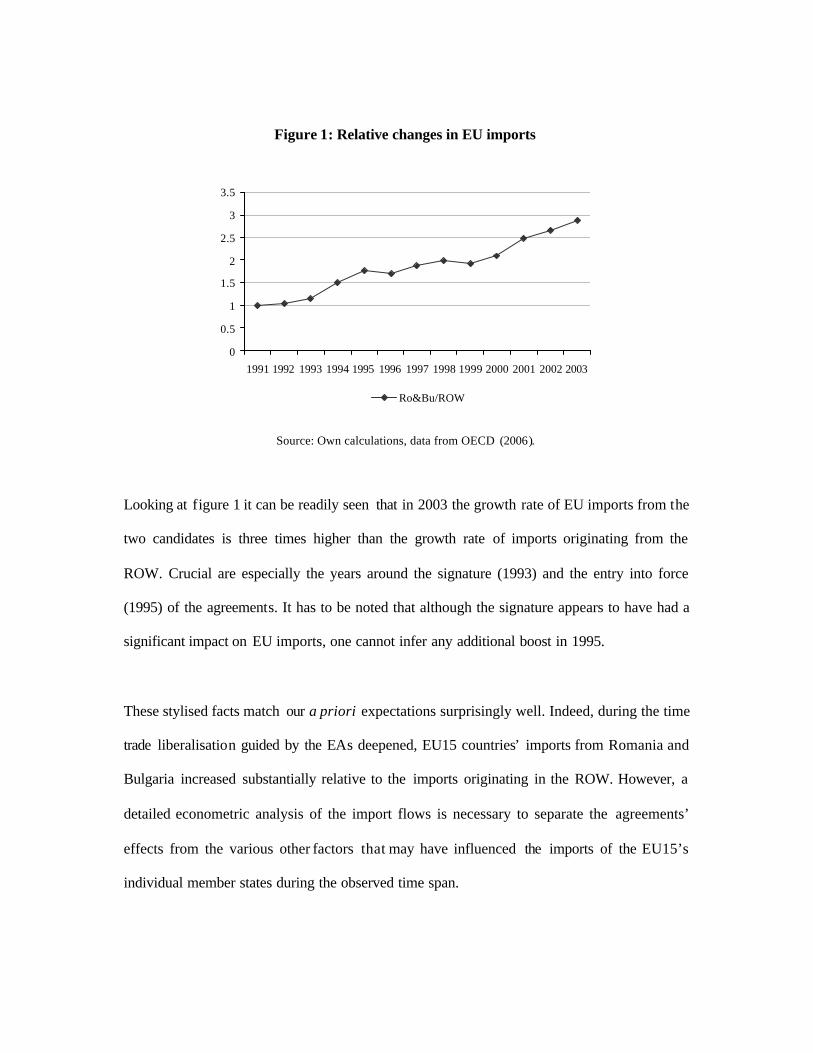
Figure 1: Relative changes in EU imports

0

0.5

1

1.5

2

2.5

3

3.5

1991 1992 1993 1994 1995 1996 1997 1998 1999 2000 2001 2002 2003

Ro&Bu/ROW

Source: Own calculations, data from OECD (2006).

Looking at figure 1 it can be readily seen that in 2003 the growth rate of EU imports from the

two candidates is three times higher than the growth rate of imports originating from the

ROW. Crucial are especially the years around the signature (1993) and the entry into force

(1995) of the agreements. It has to be noted that although the signature appears to have had a

significant impact on EU imports, one cannot infer any additional boost in 1995.

These stylised facts match our a priori expectations surprisingly well. Indeed, during the time

trade liberalisation guided by the EAs deepened, EU15 countries’ imports from Romania and

Bulgaria increased substantially relative to the imports originating in the ROW. However, a

detailed econometric analysis of the import flows is necessary to separate the agreements’

effects from the various other factors that may have influenced the imports of the EU15’s

individual member states during the observed time span.

3. On the concepts of trade creation and trade diversion

Theoretical insights in allocation effects of RTAs were first given by Viner (1950) and Byé

(1950) arguing that a fractional reduction of trade barriers leads only to a shift, but not to an

elimination of the discrimination of different sources of supply. Viner named the resulting

effects trade-creation and trade-diversion.

Trade creation is then associated with the portion of the new trade between member countries

that is wholly new resulting in an improvement in the international resource allocation. It

occurs when subsequent to the formation of a customs union, domestic production at high

costs is replaced by lower -cost sources from the new partner country. Trade diversion refers

to the part of the new trade between member countries that is only a substitute for trade with

third countries. It describes a situation in which the preferential trade liberalisation causes

higher-cost production from the new partner country to replace imports from low-cost sources

in the ROW. In this case, the resource allocation is worsened. The concepts of trade diversion

and trade creation in their original version refer only to producers and consumers inside the

RTA area. Trade diversion can, however, seriously harm excluded countries, in particular,

when they are confronted with such a large trade bloc as the EU.

Attempts to find general circumstances under which the positive effects from trade creation

surpass the negative consequences from trade diversion following the implementation of an

RTA have been subject to much controversy. One of the few surviving criteria is the natural

trading partner hypothesis, stating that an RTA among prospective members of a regional

grouping that are already major trading partners would reinforce natural trading patterns

instead of diverting them (Wonnacott and Lutz 1989). A quick look at the EU imports over

GDP ratios for the CEECs suggests that trade creation should dominate for the EAs with those

countries that were at the time of the implementation of the agreement already well integrated

into the EU (figure 2). Thus, one should expect the EAs with Slovenia, the Baltic countries

and Slovakia and the Czech Republic to be less harmful to the ROW than the EAs with

Hungary and Poland and with Romania and Bulgaria.

Figure 2: EU integration in the years of signature and entry into force of the EAs

0

0.050.1

0.15

0.2

0.25

0.3

0.35

0.4

0.45

Bulgaria

Romani

a

Czech R

epublic

Slovak

ia

Hungary

Poland

Estoni

a

Lithua

nia Latvia

Sloven

ia

Imports/GDP

Year of signature Year of entry into force 2003

Source: Own calculations, data from OECD (2006) and UN (2006).

On the other hand, one could argue that countries that were less integrated before the EAs

have benefited the most from signing them. Figure 2 reveals the biggest growth of imports

over GDP ratios for those countries that signed the EAs in the early 1990s (particularly

Slovakia, Hungary and the Czech Republic) and virtually no or even negative growth for the

Baltic countries and Slovenia, who entered into the EAs some years later (compare table A.1) .

Again, whether these gains can be attributed to the EAs must be subject to a more formal

econometric analysis.

4. Theoretical foundation of the gravity equation

Researchers use the Vinerian terms frequently when examining empirically the consequences

of preferential liberalisation for third countries. Most studies formally assessing the impact of

any kind of integration arrangement make use of the gravity equation (see e.g. Bayoumi and

Eichengreen 1995, Frankel and Wei 1998, Soloaga and Winters 2001 or for a more recent

study Carrère 2006). Even though the gravity equation’s initial success stemmed from its

good empirical properties, it possesses nowadays “more theore tical foundations than any

other trade model” (Baldwin 2006). The repeated ignorance of which has, however, produced

a number of commonly-accepted mistakes in gravity model estimation, so that we attach

importance to laying out briefly the derivation of the equation we are going to test.

Assuming identical, homothetic Constant Elasticity of Substitution (CES) preferences and

“iceberg” type transport costs, country i’s aggregate total value of imports from country j can

be expressed as

σ−

=

1

i

ijijij P

pYNM with

σ−

=

1

i

ijij P

ps (2)

with jN representing the variety of products sold by country j and iY being country i’s

nominal expenditure. i

ij

P

p is the relative price determining the share of country i’s

expenditure spent on country j’s goods ijs with iP being country i’s price index for all import-

competing goods and ijp standing for the ‘landed’ price. σ is the above-unity elasticity of

substitution between goods originating from country i and country j.3 Since prices on

individual goods are hardly available, we define the landed price

ijjijij ePtp = (3)

as a function of bilateral trade costs ijt , country j’s producer price index jP and the nominal

exchange rate ije .4 Substituting (3) into (2) yields

σ−= 1)( ijijijij retYNM (4)

with i

jijij P

Pere = as the real exchange rate. Equation (4) already looks close to commonly

estimated gravity equations. However, as stated by Anderson and van Wincoop (2003),

bilateral trade does not solely depend on bilateral trade costs, but also on the average

resistance to trade with the rest of the world. Employing general equilibrium conditions has

the convenient side effect of eliminating the number of varieties jN , for which data is not on-

hand.5 Producer prices in country j must then adjust, such that

∑=

=I

iiijjj YsNY

1

(5)

Recalling equations (2) and (3), we can solve for jN as follows:

3 Usual estimates of σ range from 5 to 8. Consequently a rise in the relative prices by 1% would cause the total import value to fall by 4 to 7%. 4 An exchange rate variable has first been formally introduced into the gravity equation by Bergstrand (1985). 5 Annex A.2 describes the case for a restricted country sample.

( )∑=

−= I

iiijij

jj

Ytre

YN

1

1 σ (6)

Plugging (6) into (4) and defining ∑=

=I

iiW YY

1

, we obtain our testable gravity equation

σ−

=

=

∑

1

1

I

iijij

ijij

W

jiij

tre

tre

Y

YYM (7)

where country i’s total imports from country j are not only dependent on the relative incomes

of the two countries but also on the bilateral exchange rate and trade cost relative to country

i’s average cost and exchange rate with respect to all other trading partners. Only by

considering these multilateral terms, it can be explained why a certain region is pushed

towards trade with a given partner when barriers towards all trade partners increase.

In line with the basic idea behind gravity models that the intensity with which a pair of

countries trades is subject to pull and push factors, we adopt a broad interpretation of the

bilateral and multilateral trade resistance terms and assume the unobservable ijt to be a log-

linear function of a set of observable variables,6

][)( 87654321 iijijijijji EAEADEPCLBLLLLijij eDt δδδδδδδδ ++++++= (8)

6 Compare Mélitz (2005) for a similar interpretation of the bilateral trade cost variable.

where ijD as the great-circle distance between the importing and the exporting country, )( jiLL

as dummy variables being equal to 1 if country i (j) is landlocked and 0 otherwise and ijB as a

dummy variable being equal to 1 if country i and j share a common border and 0 otherwise

influence trade costs by serving as proxies for a transport cost variable. Supposing that

cultural proximity beats down the landed price through transaction cost savings, the dummy

variable ijCL equals 1 when the importer and the exporter have the same official language and

0 otherwise. Finally, ijDEP is a dummy taking the value of 1 whenever country j is a non-

independent entity being legally associated with an independent state and 0 otherwise. 7

To separate the ex-post effects of the EAs with Romania and Bulgaria from those signed with

the other CEECs, a set of stepwise dummy variables has to be included into the theoretically

derived gravity equation.

ijEA = 1 for the contracting parties for the years following the signature of the EAs

and

= 2 for the years following the entry into force of the EAs (intra-bloc bias)

to capture the impact of the EAs on intra-group trade and

iEA = 1 for non-contracting parties for the years following the signature of the EAs

and

= 2 for the years following the entry into force of the EAs (extra-bloc

openness)

7 This includes French Polynesia and New Caledonia for France, Aruba and the Netherlands Antilles for the Netherlands and Bermuda and the Cayman Islands for the United Kingdom.

to capture the impact of the EAs on trade of group members with non-members.8

Following this specification, we will be able to examine whether the EAs were only trade-

creating (they caused trade between the EU and the associated countries to increase above the

normal levels without changes in trade with third countries) or trade-diverting (they increased

intra-group trade at the expense of lower trade with third countries).

While the theoretical equation (7) is remarkably close to an empirically testable gravity

equation, its estimation is problematic due to the non-linear functional form of the multilateral

trade resistance terms. Several authors therefore proposed different remoteness measures as

proxies that usually weight the average distance of a country i from the ROW with the share

of country j’s output in world output. Since there is no theoretical justification to do so, we

abstract from the inclusion of any GDP weights in constructing the multilateral resistance

variable and define

∑ ∑ ∑ ∑∑= = = = =

−+=I

i

I

i

J

j

I

i

J

jijijijij D

IJD

JD

It

1 1 1 1 1

111 (9)

The first two terms on the RHS represent the multilateral trade resistances of the respective

trading partners, and thus, boost bilateral trade between them. The last term, however,

resembles the world resistance to trade and as such, lowers the trade volume between every

pair of countries. 9

8 The countries are grouped by dates of signature and entry into force of the EAs. See table A.1 for details. 9 See Baier and Bergstrand (2006) for the theoretical derivation of multilateral and world resistance terms.

Taking into account the modifications of the theoretically derived equation discussed above,

the log-linearised10 reduced-form gravity equation boils down to

∑ ∑∑Τ

= ==

+++++++=1 1

61

5)(4321 ln1

ln(ln)lnlnlnlnδ

εββββββα ijt

C

iij

C

iijttijijtjtitijt tre

CtreYYM

(10)

where WY1 is absorbed into the constant term α 11, common to all years and all country

pairs, ijtε is the i.i.d. error term and the expected coefficient signs are

.0,0,0)1(,0)1(

,0)1(,0)1(,0)1(,0)1(,0)1(,0)1(,0,0,0

6587

16543214321

>><−>−

>−>−>−<−<−<−=<>> ∑Τ

=

ββδσδσ

δσδσδσδσδσδσββββδ

5. Econometric issues and data

In accordance to the findings of Egger (2002), panel data methodology is applied. First, and in

contrast to cross-section analysis, panels enable us to capture relevant relationships between

variables over time. Second, they allow monitoring unobservable country-pairs individual

effects. Cheng and Wall (2004) further demonstrate that not controlling for country

heterogeneity yields biased estimates. The country-pair effects will be treated as fixed, since

the random effects model only yields consistent estimates when the unobservable bilateral

effects are not correlated with the error term. The conducted Hausman test, however, rejected

null-hypothesis of no correlation. The relevant fixed effects (FE) regression thus gives

10 The brackets after 4β indicate that the dummy variables included in ijt will not be log-linearised whereas

distance of course, will. 11 Since wY is constant we implicitly assume no world growth, although countries i and j may grow. As a consequence, we assume that the positive growth of some countries is cancelled by the negative growth of others so that the world as a whole does not grow.

unbiased estimates of the time-varying variables (reported in column 1 and 2 of table 1 and 2),

nevertheless, to provide comparability, we also present the estimated parameters of the

random effects (RE) and the fixed effects vector decomposition (FEVD) regressions. The

latter has been developed by Plümper and Troeger (2004) and equals a stepwise fixed effects

estimation technique, rendering the estimation of the time-invariant variables possible . We

further detected heteroskedasticity and serial correlation of the error terms and corrected for it

in all regressions. Finally, we controlled for a possible selection bias by including three

variables that approximate the Heckman correction term: HC1 is a variable containing the

number of years of a trading pair in the sample. HC2 and HC3 are dummies, taking the value

of 1 if the trading pair is observed over the entire period 1991 to 2003 and if the trading pair is

present in the sample in t-1, respectively (and 0 otherwise). 12

As for the data, we consider EU15 countries’ imports from a worldwide sample of 204

countries over the period 1991-2003, forming an unbalanced panel data set with roughly

32194 observations. The data sources and definitions of all variables entering the tested

gravity equation are listed in table A.3 in the appendix .

6. Results

The results of the regressions with and without the multilateral resistance terms are presented

in table 1. Except for two EA dummies, all parameter estimates of the relevant fixed effects

model show the expected sign and are highly significant. This also holds true for the

multilateral resistance terms. Imports from a certain trading partner increase nearly

proportionally to a depreciation of the importing country’s currency against all other 12 The empirical estimation also contains an EU dummy, controlling for the accession of Austria, Sweden and Finland in 1995 only.

currencies. A rise in country i’s geographical distance (remoteness) from all other trading

partners pushes it to trade 44% more with country j. As for the traditional gravity variables,

the positive parameter estimates for GDP indicate that the import value increases with the

importer’s GDP raising due to a higher import demand and with the exporter ’s GDP raising

due to a higher export supply. The coefficients are, however, somewhat away from the

theoretically predicted unitary elasticity.

Moving to the fixed effects vector decomposition regression, we find that our distance

coefficient of -1.33 lies within the usual range.13 With the inclusion of the multilateral terms,

the elasticity of the import volume with respect to the GDP measures (and with respect to

distance as well) increases, endowing them with an additional justification. Note that the

theoretically justified inclusion of the real exchange rate exhibits empirical importance as

well. A 10% depreciation (e.g. a rise in the exchange rate) of the importing country’s currency

against its trading partner’s currency reduces the import value from the latter by 3.7%. Being

landlocked reduces the imports by 51% for country i and 78% for country j not having access

to the sea. Being legally dependant on the importing country more than doubles and sharing a

common language more than triples the propensity to trade.

13 The elasticity of transport costs to distance is usually associated with an estimate in the range of

4.02.0 1 << δ (Limao / Venables 2001). Combined with an average estimate of 7=σ , a distance coefficient between -1.2 and -2.4 would be suggested.

Table 1: Estimation results

FE RE FEVD w/o MR with MR w/o MR with MR w/o MR with MR

itYln 0.20** 0.44 *** 1.02*** 0.96*** 0.20*** 0.44 ***

jtYln 0.67*** 0.71 *** 1.14*** 1.15*** 0.67*** 0.71 ***

ijtreln -0.28*** -0.37*** -0.08*** -0.06*** -0.28*** -0.37***

ijDln -0.86*** -1.70*** -1.33*** -1.77***

ijB 0.00 -0.00 0.00*** 0.00***

iLL -0.47*** -0.65*** -1.11*** -0.71***

jLL -0.58*** -0.52*** -1.43*** -1.52***

ijDEP 0.74* 0.75* 0.99*** 1.12 ***

ijCL 1.39*** 1.19 *** 1.07*** 1.46 ***

iEU 0.14** 0.13** 0.43*** 0.49 *** 0.14*** 0.13 ***

irobutEA 0.25*** 0.25 *** 0.12*** 0.14 *** 0.25*** 0.25 ***

ihupotEA 0.10 0.07 0.12** 0.15** 0.10** 0.07

iczsltEA 0.71*** 0.76 *** 0.50*** 0.51 *** 0.71*** 0.76 ***

isvtEA 0.10** 0.03 0.10* 0.13*** 0.10*** 0.03

ibalticstEA 0.40*** 0.37 *** 0.44*** 0.46 *** 0.40*** 0.37 ***

itEA (Ro, Bu) -0.11*** -0.12*** -0.11*** -0.11*** -0.11** -0.12***

itEA (Hu, Po) -0.20*** -0.23*** -0.13*** -0.13*** -0.20*** -0.23***

itEA (Cz, Sl) 0.21*** 0.26*** 0.08*** 0.08** 0.21*** 0.26***

itEA (Sv) 0.02 -0.04* -0.03** -0.02 0.02 -0.04*

itEA (Baltics) 0.05** 0.02 0.01 0.01 0.05 0.02

∑=

C

iijtre

C 1

1

1.01*** -0.26*** 1.01***

∑=

C

iijt

1

0.99 *** 0.44 ***

HC1 0.49*** 0.49*** 0.66*** 0.64 *** HC2 -1.89*** -1.80*** -1.94*** -2.15*** HC3 0.11** 0.10** 0.03 0.03 0.11** 0.10* Observations 32194 32194 32194 32194 32194 32194 R-squared 0.91 0.91 0.70 0.71 0.91 0.91 * significant at 10%; ** significant at 5%; *** significant at 1%

Source: Own calculations.

The results for the EAs are very robust to the inclusion of the multilateral trade resistance

variables. The regressions display the meaningfulness of the EAs for the CEECs’ integration

into the EU. Three out of five dummy variables argue for a significant boost of the EU15

countries’ imports brought about by the agreements. Most trade has been created by the EAs

signed with the Czech Republic and Slovakia (114% above the normal level). The

arrangement also features the highest extra-bloc openness. The EAs with Hungary and Poland

exhibit the worst performance: First, the arrangements did not significantly create new trade

between the EU15 countries and Hungary and Poland. Second, the import diversion brought

about by their implementation is with 21% the highest of all EAs. The result for the Romanian

and Bulgarian agreement is somewhat mixed. While it led to 28% more imports than what

would have been predicted by the baseline-scenario gravity model, it has reduced imports

from third countries by 11%.

The trade creation and trade diversion elasticities seem to roughly confirm the natural trading

partner hypothesis introduced in section 3. The implementation of the EAs with previously

little integrated countries like Hungary and Poland as well as like Romania and Bulgaria was

not without costs for third countries. On the contrary, the Baltic countries and Slovenia (and

to a lesser extent the Czech Republic and Slovakia) were relatively well integrated into the

EU by the time of the entry into force of the agreements (compare figure 2). The estimation

results do not show any trade diversion effects for the EAs signed with these countries. The

intuition that less integrated countries profited most themselves from the EAs seems to hold

true for Romania , Bulgaria, the Czech Republic and Slovakia but not for Hungary and Poland

or the Baltic countries. The imports over GDP ratios rather support the natural trading partner

hypothesis, although the data is not very clear cut here either.

Table A.4 shows the results for different country groupings , allowing thereby for a better

comparison to previous studies. The parameter estimates underline the robustness of the

previous estimation. Taking the mean import creation generated by all individual EAs argues

for an import elasticity of 39% which is very close to the joint EA estimate of 40%. The same

holds for the coefficients of the other gravity variables.

Evaluating our results in the context of other East -West trade studies, we find that our EA

coefficient of 0.34 (thus, indicating a trade creation elasticity of 40%) lies just amidst the wide

range of previous parameter estimates (table 2).

Table 2: Trade creation elasticities in previous studies

TC elasticity Estimation technique

Adam, Kosma and McHugh (2003) 32% Panel two-step FE De Benedictis, de Santis and Vicarelli (2005) 11% Panel two-step GMM Martin and Turrion (2001) 129% Panel FE Paas (2003) -70% Cross-section

Lasser and Schrader (2002)* 266% Cross-section * Baltic states ’ imports from Belgium, Germany and the Netherlands

Source: Own illustration.

The huge differences stem from different specifications of the gravity equation, varying

estimation techniques, country samples and time spans. Closest to our procedure appear the

approaches of Adam, Kosma and McHugh (2003) and De Benedictis, de Santis and Vicarelli

(2005). The smaller elasticity of the former may stem from the fact that the authors used

exports instead of imports and also from distinct time spans. They also include only 5 years

from 1996 to 2000 into their regression and are, thus, not able to capture the entire signature

effect of the agreements. While using a similar time span to ours, De Benedictis, de Santis and

Vicarelli (2005) leave Romania and Bulgaria out of their focus. The estimate they provide

does therefore not contain, the trade created by the EA with these two countries. Finally, both

studies rely on time-invariant country (pair)-specific fixed effects to account for the

multilateral resistance terms. Since part of the resistance, namely the average exchange rate, is

time varying, however, the results are likely to be biased.

7. Conclusions

This paper has paid particular importance to theoretically deriving a new version of a

correctly specified gravity equation to avoid biases present in previous studies. We were able

to show that the frequently employed exchange rate variables do stand on a sound theoretical

ground and exhibit econometric importance. In addition, new measures for multilateral trade

resistance were introduced and showed the expected coefficient signs in the empirical

estimation.

As for the trade effects of the EAs, our result for the aggregate EA dummy is well in line with

previous estimates by Adam, Kosma and McHugh (2003). Looking at the agreements on an

individual country basis gives additional important insights: The EAs have supported and

accelerated the CEECs’ integration into the EU. The process has not been free of charge,

however. We find evidence that although each EA created new trade within the trade bloc, the

increase has in the case of Romania and Bulgaria (as well as Hungary and Poland) been at the

expense of imports from the ROW. The fact that these countries were not well integrated with

the EU at the time of the entry into force of the agreements gives some support to the natural

trading partner hypothesis.

References

Adam, A. / Kosma, D. / McHugh, J. (2003): Trade -Liberalization Strategies What Could

Southeastern Europe Learn from CEFTA and BFTA?, IMF Working Papers, no. 239.

Anderson, J. / van Wincoop, E. (2003): Gravity with Gravitas: A solution to the Border

Puzzle, in: American Economic Review, vol. 93(1), pp. 170-192.

Baier, S. / Bergstrand, J. (2006): Bonus Vetus OLS: A Simple Approach for Addressing the

“Border Puzzle” and Other Gravity-Equation Issues, at:

http://www.nd.edu/~jbergstr/Working_Papers/BVOLSMarch2006.pdf.

Baldwin, R. (2006): The Euro’s Trade Effects, ECB Working Papers, no. 594.

Bayoumi, T. /Eichengreen, B. (1995): Is Regionalism Simply a Diversion? Evidence f rom the

Evolution of the EC and EFTA, NBER Working Papers, no. 5283.

Bergstrand, J. (1985): The Gravity Equation in International Trade: Some Microeconomic

Foundations and Empirical Evidence, in: Review of Economics & Statistics, vol. 67(3), pp.

474-481.

Böcker, A. (2002): The Establishment Provisions of the Europe Agreements: Implementation

and Mobilisation in Germany and the Netherlands, ZERP Discussion Papers, no. 1.

Byé, M. (1950): Unions Douanières et Données Nationales, in : Economie appliquée, vol. 3,

pp. 121-157.

Carrère, C. (2006): Revisiting the Effects of Regional Trade Agreements on Trade Flows with

Proper Specification of the Gravity Model, in: European Economic Review, vol. 50, pp. 223-

247.

Cheng, I. / Wall, H. (2004): Controlling for Heterogeneity in Gravity Models of Trade and

Integration, Federal Reserve Bank of St. Louis Working Papers, no. 1999-010E.

Clausing, K. (2001): Trade Creation and Trade Diversion in the Canada – United States Free

Trade Agreement, in: Canadian Journal of Economics, vol. 34(3), pp. 677-696.

De Benedictis, L. / De Santis, R. / Vicarelli, C. (2005): Hub-and-Spoke or Else? Free Trade

Agreements in the Enlarged EU, in: European Journal of Comparative Economics, vol. 2(2),

pp. 245-260.

Egger, P. (2002): An Econometric View on the Estimation of Gravity Models and the

Calculation of Trade Potentials, in: The World Economy, vol. 25, pp. 297-312.

Frankel, J. / Wei, S. (1998): Open Regionalism in a World of Continental Trade Blocs, IMF

Working Papers, no. 10.

Lasser, C. / Schrader, K. (2002): European Integration and Changing Trade Patterns: The

Case of the Baltic States, Kiel Working Papers, no. 1088.

Limao, N. / Venables, A. (2001): Infrastructure, Geographical Disadvantage and Transport

Costs, World Bank Working Papers, no. 2257.

Martín, C. / Turrión, J. (2001): The Trade Impact of the Integration of the Central and Eastern

European Countries on the European Union, European Economy Group Working Papers, no.

11.

Mélitz, J. (2005): North, South and Distance in the Gravity Model, CEPR Discussion Papers,

no. 5136.

Paas, T. (2003): Regional Integration and International Trade in the Context of EU Eastward

Enlargement, HWWA Discussion Papers, no. 218.

Plümper, T. / Troeger, V. (2004): The Estimation of Time-Invariant Variables in Panel

Analyses with Unit Fixed Effects, in:

http://polmeth.wustl.edu/workingpapers.php?year=2004.

Soloaga, I. / Winters, A. (2001): Regionalism in the Nineties: What Effect on Trade?, CEPR

Discussion Papers, no. 2183.

Viner, J. (1950): The Customs Unions Issue, New York.

Wonnacott, P. / Lutz, M. (1989): Is there a Case for Free Trade Areas?, in: Schott, J. (ed.):

Free Trade Areas and US Trade Policy, Washington DC, pp. 59-84.

Appendix

Table A.1: Dates of signature and entry into force of the EAs

Dummy Country Signature Entry into force

Hungary December 1991 February 1994 hupoEA Poland December 1991 February 1994 Czech Republic October 1993 February 1995 czslEA Slovakia October 1993 February 1995 Romania February 1993 February 1995 robuEA Bulgaria March 1993 February 1995 Estonia June 1995 February 1998 Lithuania June 1995 February 1998 balticsEA

Latvia June 1995 February 1998 svEA Slovenia June 1996 February 1999 Source: Böcker (2002).

A.2: Adjusting the model to a limited number of importing countries

In this study, we have to adjust our theoretical framework to the case of EU15 countries’

imports (countries i) from a worldwide sample of countries (countries j). Say, that there exist r

other importing countries ∑∑∑===

−=I

ii

J

jj

R

rr countrycountrycountry

111

, whose import prices can

be described analogously to country i as

rjjrjrj ePtp = (A.1)

Under general equilibrium conditions, output in country j must then equal the aggregate

expenditure spent by countries i and r on varieties produced in j,

∑ ∑= =

+=I

i

R

rrrjiijjj YsYsNY

1 1

)( (A.2)

Making a few mathematical transformations, we can solve for jN

∑ ∑= =

−− +=

I

i

R

rrrjrjiijij

jj

YtreYtre

YN

1 1

11 )()( σσ (A.3)

Plugging (A.3) into (1), country i’s imports arise as

σ

σ

σ

−

=

=

=

−

=

−

+

=

∑∑

∑

∑

1

1

1

1

1

1

1

)(

)(I

iijij

ijij

I

iirI

iijij

R

rrjrj

jiij

tre

ret

YYtre

tre

YYM

For our empirical estimation this means that

∑∑

∑=

=

−

=

−

+I

iirI

iijij

R

rrjrj

YYtre

tre

1

1

1

1

1

)(

)(

1

σ

σ

will be absorbed in the

constant. E.g., we assume a co-movement of the average exchange rate and trade costs of

country r against j and the average exchange rate and trade costs of country i against j as well

as a constant world GDP.

Table A.3: List of variables

Variable Definition Source

ijtM Yearly imports of country i from country j

OECD ITCS

tjiY )( Importer and exporter GDP (in current US$)

UN NAMAD

ijtre Bilateral real exchange rate UN NAMAD (nom. exchange rates), IMF IFS (price indices and GDP deflators), own calculations 14

ijD Great circle distances between the respective trading pairs

CIA World Factbook, own calculations based on the harvesine formula

)( jiLL Dummy = 1 if the country is landlocked

CIA World Factbook

ijB Dummy = 1 if the county shares a common border with the EU

Wikipedia

ijDEP Dummy = 1 if country j legally depends on country i

CIA World Factbook

ijCL Dummy = 1 if the trading partners share a common official language

Wikipedia

ijtEA Dummy = 1 for contracting parties for the years following the signature and = 2 for the years following the implementation of the EAs

ZERP

itEA Dummy = 1 for non-contracting parties for the years following the signature and = 2 for the years following the implementation of the EAs

ZERP

14 When available the producer or consumer price index has been used for the calculation of the real exchange rate, in all other cases we reverted to the GDP deflator.

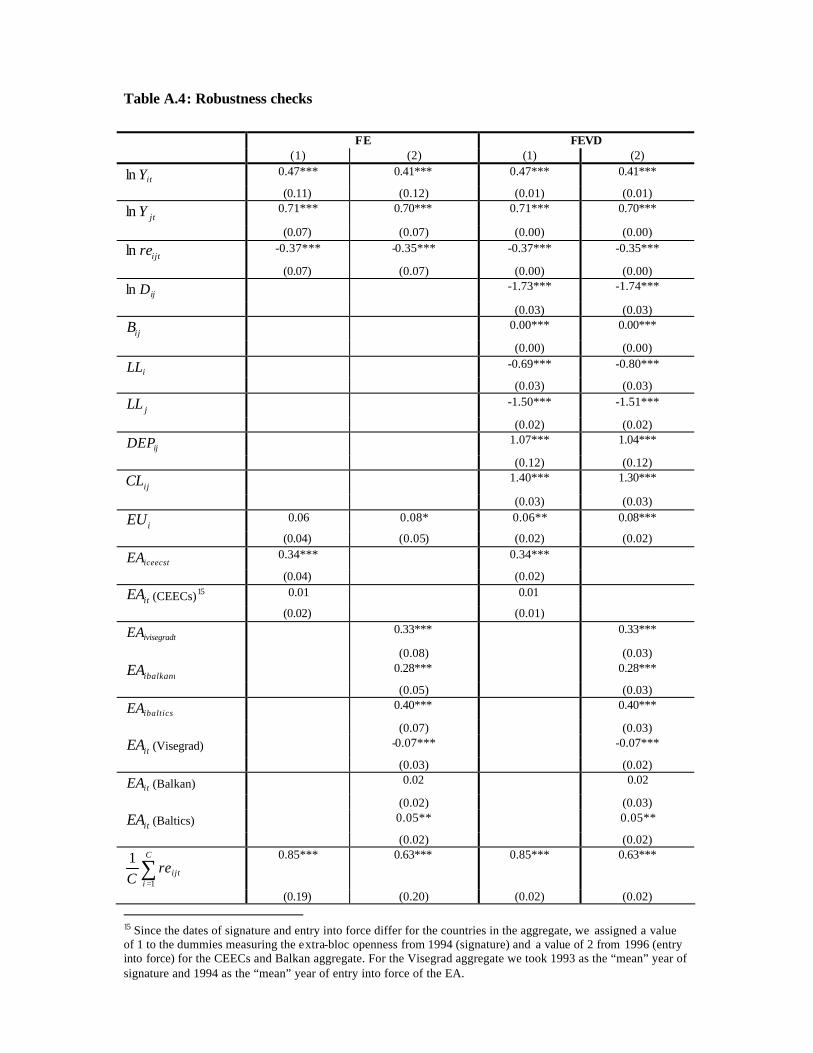
Table A.4: Robustness checks

FE FEVD (1) (2) (1) (2)

itYln 0.47*** 0.41*** 0.47*** 0.41***

(0.11) (0.12) (0.01) (0.01)

jtYln 0.71*** 0.70*** 0.71*** 0.70***

(0.07) (0.07) (0.00) (0.00)

ijtreln -0.37*** -0.35*** -0.37*** -0.35***

(0.07) (0.07) (0.00) (0.00) ijDln -1.73*** -1.74***

(0.03) (0.03) ijB 0.00*** 0.00***

(0.00) (0.00)

iLL -0.69*** -0.80***

(0.03) (0.03)

jLL -1.50*** -1.51***

(0.02) (0.02) ijDEP 1.07*** 1.04***

(0.12) (0.12)

ijCL 1.40*** 1.30***

(0.03) (0.03)

iEU 0.06 0.08* 0.06** 0.08*** (0.04) (0.05) (0.02) (0.02)

iceecstEA 0.34*** 0.34***

(0.04) (0.02)

itEA (CEECs)15 0.01 0.01

(0.02) (0.01)

ivisegradtEA 0.33*** 0.33***

(0.08) (0.03)

ibalkantEA 0.28*** 0.28***

(0.05) (0.03)

ibalticstEA 0.40*** 0.40***

(0.07) (0.03)

itEA (Visegrad) -0.07*** -0.07*** (0.03) (0.02)

itEA (Balkan) 0.02 0.02

(0.02) (0.03) itEA (Baltics) 0.05** 0.05**

(0.02) (0.02)

∑=

C

iijtre

C 1

1

0.85*** 0.63*** 0.85*** 0.63***

(0.19) (0.20) (0.02) (0.02) 15 Since the dates of signature and entry into force differ for the countries in the aggregate, we assigned a value of 1 to the dummies measuring the extra-bloc openness from 1994 (signature) and a value of 2 from 1996 (entry into force) for the CEECs and Balkan aggregate. For the Visegrad aggregate we took 1993 as the “mean” year of signature and 1994 as the “mean” year of entry into force of the EA.

∑=

C

iijt

1

0.39*** 0.41***

(0.04) (0.04) HC1 0.62*** 0.63*** (0.01) (0.01) HC2 -2.07*** -2.03*** (0.05) (0.05) HC3 -0.07** -0.03 -0.07* -0.03 (0.03) (0.03) (0.04) (0.05) Observations 32194 32194 32194 32194 R-squared 0.91 0.91 0.91 0.91 Robust standard errors in parentheses * significant at 10%; ** significant at 5%; *** significant at 1%

Source: Own calculations.