NBER WORKING PAPER SERIES

TRADE AND INVESTMENT IN THE GLOBAL ECONOMY

James E. AndersonMario Larch

Yoto V. Yotov

Working Paper 23757http://www.nber.org/papers/w23757

NATIONAL BUREAU OF ECONOMIC RESEARCH1050 Massachusetts Avenue

Cambridge, MA 02138August 2017

Part of this research has been supported by Global Affairs Canada. The views expressed herein are those of the authors and do not necessarily reflect the views of the National Bureau of Economic Research and of Global Affairs Canada. All errors are our own.

NBER working papers are circulated for discussion and comment purposes. They have not been peer-reviewed or been subject to the review by the NBER Board of Directors that accompanies official NBER publications.

© 2017 by James E. Anderson, Mario Larch, and Yoto V. Yotov. All rights reserved. Short sections of text, not to exceed two paragraphs, may be quoted without explicit permission provided that full credit, including © notice, is given to the source.

Trade and Investment in the Global EconomyJames E. Anderson, Mario Larch, and Yoto V. YotovNBER Working Paper No. 23757August 2017JEL No. F10,F43

ABSTRACT

We develop a dynamic multi-country trade model with foreign direct investment (FDI) in the form of non-rival technology capital. The model nests structural gravity sub-systems for FDI and trade, with accumulation/decumulation of phyisical and technology capital in transition to the steady state. The empirical importance of the FDI channel is demonstrated comparing actual aggregate cross-section data for 89 countries in 2011 to a hypothetical world without FDI. The gains from FDI amount to 9\%of world's welfare and to 11% of world's trade, unevenly distributed among winners and losers. Net exports of FDI substitute for export trade in the results.

James E. AndersonDepartment of EconomicsBoston CollegeChestnut Hill, MA 02467and NBERjames.anderson.1@bc.edu

Mario LarchUniversity of BayreuthUniveritaetstrasse 3095447 Bayreuth, Germanymario.larch@uni-bayreuth.de

Yoto V. YotovSchool of EconomicsDrexel UniversityPhiladelphia, PA 19104and ERI-BASyotov@drexel.edu

“Foreign direct investment (FDI) is an integral part of an open and effective in-ternational economic system and a major catalyst to development. [...] Withmost FDI flows originating from OECD countries, developed countries can con-tribute to advancing this agenda. They can facilitate developing countries’ accessto international markets and technology.”

OECD (2002)

“Today, FDI is not only about capital, but also –and more important– about tech-nology and know-how, [...] International patterns of production are leading tonew forms of cross-border investment, in which foreign investors share their in-tangible assets such as know-how or brands in conjunction with local capital ortangible assets of domestic investors.”

The World Bank (2015)

1 Introduction and Motivation

Foreign Direct Investment (FDI) is viewed as a key driver of prosperity in policy circles.

For example, FDI had a prominent role in many recent integration agreements such as

Transatlantic Trade and Investment Partnership (TTIP).1 Moreover, both opening quotes

demonstrate concern for FDI as transfers of intangible assets such as know-how, brands,

patents, etc. in addition to traditional forms of FDI as physical capital. Policy makers’

enthusiasm is based on the obvious partial equilibrium evidence of FDI impacts on sectoral

output, employment and capital returns, but there is relatively little structural evidence

for the economy-wide importance of FDI and its role in knowledge transfer. This paper

generates evidence on the importance of FDI from counter-factual simulation of a dynamic

multi-country general equilibrium model with costly international trade and investment.

The model traces the relationships between trade, domestic investment in physical capital

accumulation, and FDI in the form of technology capital. On the trade side, our model is1Policy makers and academics alike see high potential and promise that such agreements will not only

liberalize trade but also facilitate FDI. For example, on the policy side, EU analysts hope that TTIP will“liberalise trade and investment between the EU and the US and will result in more jobs and growth.” (Pressrelease, Brussels, 28 January 2014). Academics share the hopes for positive impact of integration agreementson welfare through FDI. “If successfully negotiated, [TTIP and TPP] would deepen and strengthen ties withmany of the most significant U.S. economic partners. A large majority of inward FDI in the United Statesalready originates from TTIP and TPP countries, making these deals particularly important in the broadereffort to recruit global business investment.” (p. 3, Slaughter, 2013).

1

a member of the wide class of new quantitative general equilibrium trade models described

in detail by Arkolakis et al. (2012). The novelty of our theory comes on the supply side.

Production uses FDI in the form of non-rival technology capital along with labor and physical

capital stocks. Thus countries can use their technology capital in potentially all countries

while using at home the technology capital of potentially all countries.2

A byproduct of our model is an intuitive structural FDI gravity system that very much

resembles the traditional gravity system from the trade literature. First, the value of FDI

stock is proportional to the size of the country of origin, as measured by expenditure. The

intuition for this result is that expenditure in the country of origin is proportional to the

value of marginal product of technology capital. Second, bilateral FDI is proportional to

the size of the host country, as measured by nominal output. The intuition for this result

is that nominal output is proportional to the returns to FDI in the host country. Third,

the stock value of FDI is inversely related to FDI barriers. Fourth, bilateral FDI stock

values are linked to trade via the inward multilateral resistance (IMR) in an intuitive way.

Specifically, higher IMRs in the country of origin lead to less FDI. The intuition for this

result is that higher IMRs mean higher direct and opportunity cost of investing in technology

capital. We view the structural interdependence between trade and FDI in our model as an

important contribution to the existing FDI literature, where, despite significant interest, the

relationships between trade and FDI are not clearly established. Finally, our theory suggests

that the value of FDI stock is inversely related to the amount of technology capital in the

country of its origin. This relationship is also intuitive because it is a reflection of the law

of diminishing returns to investment into technology capital.

FDI liberalization increases FDI, with interesting implications for trade, income, and2In the spirit of McGrattan and Prescott (2009, 2010, 2014) and McGrattan and Waddle (2017) we

characterize technology capital as ‘non-rival’. However, our interpretation of technology capital is alsoconsistent with the notion of ‘jointness’ of capital from Markusen (2002), who defines ‘jointness’ as “theability to use the engineer or other headquarters asset in multiple production locations without reducingthe services provided in any single location. A blueprint is the classical example of a joint input. Jointnessinherently refers to the costs of running two plants rather than one.” Markusen (2002, p. 130). Thus,depending on preference, throughout the analysis the reader may use the terms ‘non-rival technology capital’and ‘joint technology capital’ interchangeably.

2

expenditure. An increase in bilateral FDI directly leads to higher income and to higher

expenditure in the liberalizing countries. Since higher expenditure leads to more accumula-

tion of technology capital, FDI liberalization between two countries will also trigger positive

spillover effects on output and expenditure in third countries. Through its impact on output

and expenditure, increases in FDI will also translate into increases in trade flows. Moreover,

the changes in FDI will affect trade indirectly, by the effect of outputs and expenditures on

the multilateral resistances. Finally, since multilateral resistances are general equilibrium

indexes, i.e. they capture the effects of trade liberalization between any two countries on

consumer and on producer prices in any other country in the model, the FDI changes will

transmit throughout the world.

The results of the counterfactual comparative (steady state) statics show that net export

of FDI substitutes for export trade. The modular structure of the model allows an intuitive

explanation, despite the unavailability of analytic results. In partial equilibrium with incomes

held constant, net FDI importers pay for their use of foreign technology on balance, hence

elimination of FDI raises expenditure to the level of income. The share of income spent on

home goods rises so exports must fall. Net FDI exporters lose net payments from foreign

users, hence elimination of FDI lowers expenditure to the constant level of income. The

share of income spent on home goods falls, so exports must rise. A general equilibrium

force modifies partial equilibrium insight for countries with large (in absolute value) net FDI

positions. Net exporters of FDI lose income from FDI elimination (less technology capital is

accumulated in response to loss of technology capital exports) while net FDI importers gain

income (more domestic technology capital is accumulated in response to absence of foreign

technology capital). This force dampens the partial effects but does not eliminate it.

Trade and trade liberalization affect FDI via two channels in our model. First, changes in

trade costs lead to changes in expenditure, which in turn shift the value of marginal product

of FDI and thus directly affect investment in technology capital. Second, trade liberalization

shifts prices, which affects both FDI and trade. Specifically, FDI is inversely related to the

3

prices of consumer and investment goods in the country of origin, because these prices are

part of the direct and the opportunity costs, respectively, of investment in technology capital.

To the extent that trade liberalization leads to increased expenditure and to lower prices of

consumption and investment goods, our model predicts that lower trade costs will stimulate

the accumulation of technology capital in the liberalizing countries. Moreover, the increased

stock of technology capital in the liberalizing countries will lead to positive spillover effects

in the rest of the world, due to the non-rival nature of technology.

The empirical importance of the novel FDI channel is demonstrated in a counterfactual

experiment that describes a hypothetical world without FDI. Three main findings stand out.

First, we establish that FDI is indeed an important component of the modern world eco-

nomic system. Our estimates reveal that, on average, the gains from FDI amount to 9% of

world’s welfare and to 11% of world’s trade in 2011, which is the year of our counterfactual

analysis. Second, we find that the impact of FDI has been very heterogeneous across the 89

countries in our data. While most countries in the world have benefitted from FDI, some

have incurred losses due to FDI. We offer a series of explanations for this result. Third,

the large magnitude of the FDI effects combines with its wide hetorogeneity to suggest im-

plications of FDI for changes in cross-country income inequality. For example, our results

suggest that FDI has led to significant increases in the real GDP and the welfare of some of

the poorest economies in the European Union. Given the renewed interest in the determi-

nants of inequality, cf. European Commission (2010), our results have potentially important

implications for regional policy.

Our work is related to several prominent strands in the literature. Our model nests

the standard structural gravity model of trade, so its static module is a member of the

wide class of quantitative general equilibrium (GE) trade models described by Arkolakis

et al. (2012) and Costinot and Rodríguez-Clare (2014). The dynamic model of domestic

investment in the form of physical capital accumulation is in the spirit of Olivero and Yotov

4

(2012), Anderson et al. (2015) and Eaton et al. (2016).3 The novelty in our analysis adds

to the previous static and dynamic GE trade models by allowing for FDI on the transition

to a steady (stationary) state. Thus, our work is related to the literature that studies

the determinants and implications of foreign direct investment.4 Following McGrattan and

Prescott (2009, 2010, 2014) and McGrattan and Waddle (2017), and motivated by empirical

evidence, FDI takes the form of non-rival technology capital.5 Relative to McGrattan et

al., our methodological contribution is the modeling of the joint interactions between FDI

and bilateral trade in an asymmetric many country world. Finally, our work contributes to

the empirical literature that studies the determinants of FDI, e.g. Eicher et al. (2012) and

Blonigen and Piger (2014). Even though FDI estimations are beyond the scope of this study,

we believe that, owing to its similarities with the very successful gravity system of trade, our

structural FDI gravity system will be useful to researchers and policy makers.

The remainder of the paper is organized as follows. Section 2 develops the theoretical

framework. This section also introduces the structural FDI gravity system as a byproduct

of our model. Section 3 presents the empirical analysis. Section 3.1 describes the data

and the calibration methods and parameters, while Section 3.2 presents and discusses our

main findings of the counterfactual analysis. Section 4 concludes and offers directions for

improvements and extensions.3The empirical relevance of physical capital accumulation as a key determinant of various economic

outcomes is demonstrated in Wacziarg (2001), Baldwin and Seghezza (2008), Wacziarg and Welch (2008),and Cuñat and Maffezzoli (2007).

4Related FDI papers include Head and Ries (2008) and Bergstrand and Egger (2007, 2010). In addition,we refer the reader to Antras and Yeaple (2014) for an excellent survey of the literature on the decisions ofmultinational firms.

5As noted earlier, our interpretation of technology capital is akin to the ‘jointness’ of knowledge capital(i.e. patents, blue-prints, management skills/practices, etc.) from Markusen (1997, 2002) and Markusen andMaskus (2002). Sampson (2016) models non-rival technology capital accumulation with dynamic selectionof heterogeneous firms in a highly symmetric setting with uniform country size and uniform trade costs.

5

2 Theoretical Foundation

We build a dynamic model of trade, domestic capital accumulation and foreign direct in-

vestment. The world consists of N countries, and each of them produces a single tradeable

good, differentiated by place of origin. Each country purchases goods from every source (as

in Armington, 1969), which are used for final consumption and for domestic investment in

physical and non-rival technology capital that may be ‘leased’ to all other countries. The

quotes enclosing ‘leased’ connote that technology transfer includes both within firm Foreign

Direct Investment (FDI) and arms length licensed technology transfer, equivalently leading

to payments across borders for the use of technology.6 Following McGrattan and Prescott

(2009), we abstract from FDI in the form of physical means of production. The basic building

blocks are set out below.

Production. Total nominal output in country j at time t (Yj,t) is produced subject to the

following constant returns to scale (CRS) Cobb-Douglas production function:

Yj,t = pj,tAj,t(L1−αj,t Kα

j,t

)1−φMφj,t α, φ ∈ (0, 1), (1)

where pj,t denotes the factory-gate price of good (country) j at time t. Production in country

j at time t relies on local technology (Aj,t), global technology stock applied locally (Mj,t)

and country-specific (internationally immobile) resources including labor endowment (Lj,t)

and physical capital stock (Kj,t).

Technology capital is ‘non-rival’ or ‘joint’, i.e. country i can use its technology capital

(Mi,t) at home and in all other countries. Possible examples include patents, blue-prints,

management skills/practices, etc. Formally global technology capital Mj,t applied in j at6Payments by affiliates for use of parent firm technology often differ from the true internal value, for

tax and strategic reasons beyond the scope of this study, so the neutral term ‘licensing’ is used to moreaccurately describe the economically relevant value of the technology transfer.

6

time t in production function (1) is defined as

Mj,t ≡

(N∏i=1

(max1, ωij,tMi,t)ηi), (2)

comprising domestic technology capital Mj,t and foreign direct investments:

FDIij,t ≡ ωij,tMi,t. (3)

Here, Mi,t is the technology capital stock in country i at time t, and ωij,t measures the

openness for foreign technology of country i in country j at time t, thus encompassing all

possible bilateral FDI frictions between i and j. If ωij,t = 0, no foreign technology from

country i can be used in country j at time t. If ωij,t > 0, then every unit of foreign

technology from country i at time t has ωij,t-times the use in country j.7 Finally, constant

returns to scale is imposed by∑N

i=1 ηi = 1. The max-function, which we use to introduce

FDI as a component in national production implements the notion that there is some world

knowledge of technology capital freely available to all countries and normalized to one. The

stock of world knowledge is normalized in the second argument of the max-function. A

technical advantage of the max-function is that it ensures that we can capture zero bilateral

FDI flows between countries, which we observe regularly in the data.8

Physical capital in each country accumulates according to a standard linear transition

function:

Kj,t+1 = (1− δK)Kj,t + Ωj,t, (4)

where δK are the physical capital adjustment costs and Ωj,t denotes the aggregate flow of

investment in physical capital in country j at time t, which we model as a CES aggregate of7The FDI frictions are “dark” like iceberg trade costs. Sampson (2016) lays out a dynamic selection device

for heterogeneous firms that potentially lights some of the darkness.8Our approach is similar to McGrattan and Prescott (2009, 2010). In Appendix B we provide an alter-

native specification where technology capital across all countries is as in McGrattan and Prescott (2009)summed rather than combined via a Cobb-Douglas function.

7

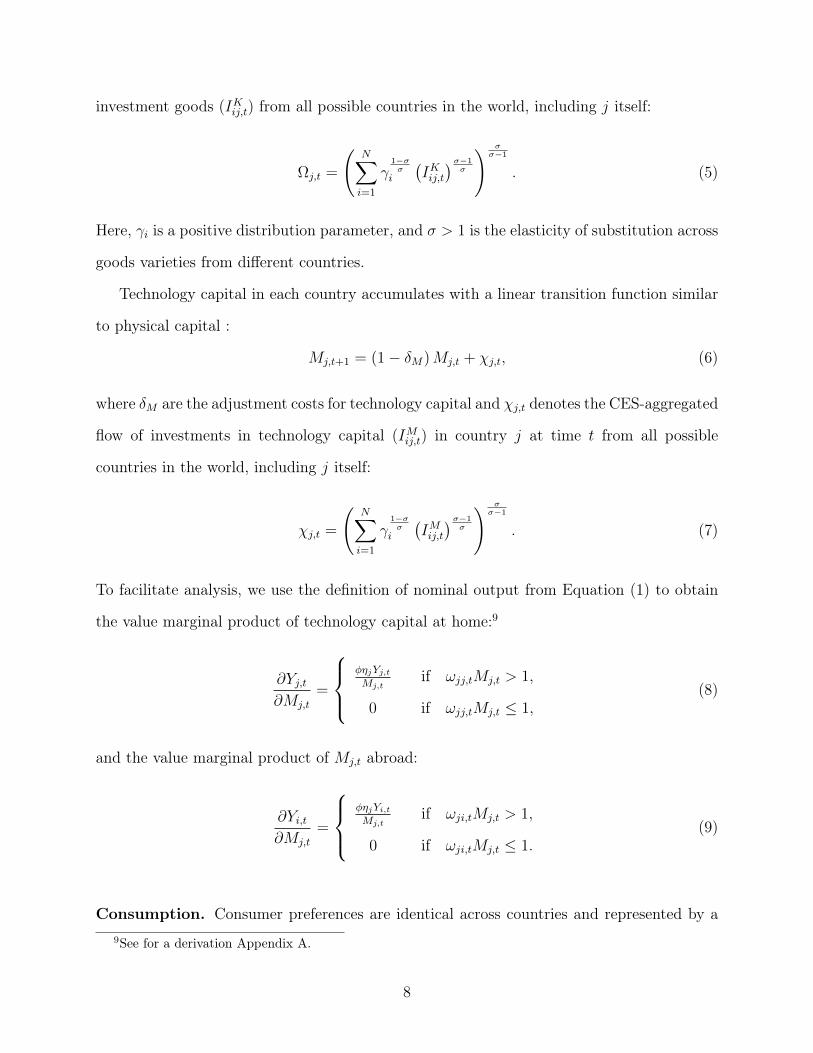
investment goods (IKij,t) from all possible countries in the world, including j itself:

Ωj,t =

(N∑i=1

γ1−σσ

i

(IKij,t)σ−1

σ

) σσ−1

. (5)

Here, γi is a positive distribution parameter, and σ > 1 is the elasticity of substitution across

goods varieties from different countries.

Technology capital in each country accumulates with a linear transition function similar

to physical capital :

Mj,t+1 = (1− δM)Mj,t + χj,t, (6)

where δM are the adjustment costs for technology capital and χj,t denotes the CES-aggregated

flow of investments in technology capital (IMij,t) in country j at time t from all possible

countries in the world, including j itself:

χj,t =

(N∑i=1

γ1−σσ

i

(IMij,t)σ−1

σ

) σσ−1

. (7)

To facilitate analysis, we use the definition of nominal output from Equation (1) to obtain

the value marginal product of technology capital at home:9

∂Yj,t∂Mj,t

=

φηjYj,tMj,t

if ωjj,tMj,t > 1,

0 if ωjj,tMj,t ≤ 1,(8)

and the value marginal product of Mj,t abroad:

∂Yi,t∂Mj,t

=

φηjYi,tMj,t

if ωji,tMj,t > 1,

0 if ωji,tMj,t ≤ 1.(9)

Consumption. Consumer preferences are identical across countries and represented by a9See for a derivation Appendix A.

8

logarithmic utility function with a subjective discount factor β < 1:

Uj,t =

∞∑t=0

βt ln(Cj,t), (10)

where aggregate consumption (Cj,t) includes domestic and foreign goods (cij,t) from all pos-

sible countries in the world, including country j, subject to:

Cj,t =

(N∑i=1

γ1−σσ

i cσ−1σ

ij,t

) σσ−1

. (11)

The assumption that consumption and investment goods are both a combination of all world

varieties subject to the same CES aggregation is very convenient analytically. Allowing for

heterogeneity in preferences and prices between and within consumption and investment

goods will open additional channels for the interaction between trade, FDI and domestic

investment. However, such treatment requires the introduction of an additional sectoral

dimension which is beyond the scope of this project.

Agent’s Problem. Representative agents in each country work, invest and consume. At

every point in time consumers in country j choose aggregate consumption (Cj,t) and aggre-

gate investment into physical (Ωj,t) and technology (χj,t) capital to maximize the present

9

discounted value of lifetime utility subject to a sequence of constraints:

maxCj,t,Ωj,t,χj,t

∞∑t=0

βt ln(Cj,t) (12)

Kj,t+1 = (1− δK)Kj,t + Ωj,t for all t, (13)

Mj,t+1 = (1− δM)Mj,t + χj,t for all t, (14)

Yj,t = pj,tAj,t(L1−αj,t Kα

j,t

)1−φ(

N∏i=1

(max1, ωij,tMi,t)ηi)φ

for all t, (15)

Ej,t = Pj,tCj,t + Pj,tΩj,t + Pj,tχj,t for all t, (16)

Ej,t = Yj,t + φηj∑i∈Nji,t

Yi,t − φYj,t∑i∈Nij,t

ηi for all t, (17)

Kj,0 , Mj,0 given. (18)

Here, for expositional convenience, we have defined a set of constraints Nij,t ≡ i 6= j, ωij,tMi,t

> 1. Equation (12) is the representative agent’s intertemporal utility function. Equations

(13), (14) and (15) define the law of motion for physical capital stock, the law of motion for

technology capital stock, and the value of production, respectively. Equation (16) gives total

spending in country j at time t, Ej,t, as the sum of spending on consumption (Pj,tCj,t), spend-

ing on investments in physical capital (Pj,tΩj,t), and spending on investments in technology

capital (Pj,tχj,t). Finally, Equation (17) defines disposable income as the sum of total nominal

output (Yj,t) plus rents from foreign investments(φηj

∑i∈Nji,t Yi,t =

∑i∈Nji,tMj,t × ∂Yi,t

∂Mj,t

),

minus rents accruing to foreign investments(φYj,t

∑i∈Nij,t ηi =

∑i∈Nij,tMi,t × ∂Yj,t

∂Mi,t

), as de-

fined in Equations (8) and (9), respectively.

2.1 A Model of Trade and Investment

Solving the representative agent’s problem delivers a structural system that describes the

relationships between trade, domestic investment and FDI. We solve the agent’s optimization

problem in two steps. First, we solve the optimal demand of cij,t, IKij,t and IMij,t for given

aggregate variables. Following Anderson et al. (2015), we label this stage the ‘lower level ’.

10

Then, we solve the dynamic optimization problem for Cj,t, Ωj,t and χj,t. This is what we call

the ‘upper level ’.

‘Lower Level’ Equilibrium. Let pij,t = pi,ttij,t denote the delivered price of country

i’s goods for country j consumers, where tij,t is the variable bilateral trade cost factor on

shipments from i to j at time t.10 Let Xij,t = pij,t(cij,t + IKij,t + IMij,t) denote country j’s total

nominal spending on goods from country i at time t. Solving the representative agent’s

optimization of (5), (7), and (11), subject to (16) and taking Cj,t, Ωj,t, and χj,t for all j as

given, delivers the familiar structural system of Anderson and van Wincoop (2003):

Xij,t =Yi,tEj,tYt

(tij,t

Πi,tPj,t

)1−σ

, (19)

P 1−σj,t =

N∑i=1

(tij,tΠi,t

)1−σYi,tYt, (20)

Π1−σi,t =

N∑j=1

(tij,tPj,t

)1−σEj,tYt

. (21)

In terms of notation, system (19)-(21) is virtually identical to the original structural gravity

system of Anderson and van Wincoop (2003) and, therefore, it is representative of the whole

family of micro-founded gravity models described by Arkolakis et al. (2012). The introduc-

tion of FDI implies that Yi,t 6= Ei,t. In turn, this means that in our framework trade and

prices respond endogenously to changes in FDI. This will become clear next, when we solve

for the ‘upper level ’ equilibrium in our model.

‘Upper Level’ Equilibrium. Our model of trade, domestic capital accumulation, and FDI

does not have analytical solutions for the transition functions for physical and technology

capital. Thus we analyze the steady-state in order to be able to offer a clear discussion of the

key structural relationships and mechanisms in our framework. To solve for the upper level10Trade costs thus can be interpreted by the standard iceberg melting metaphor: It is as if goods melt

away in distribution so that 1 unit shipped becomes 1/tij,t < 1 units on arrival. Technologically, a unit ofdistribution services required to ship goods uses resources in the same proportions as does production. Theunits of distribution services required on each link vary bilaterally.

11

steady state equilibrium, we set up the Lagrangian and we obtain the first order conditions for

the key variables in our model, including the first order condition for physical capital and the

first-order condition for technology capital.11 Then, we combine the first-order conditions

with the production function, the budget constraint, the expressions for expenditure and

factory-gate prices, and the equations from the lower-level equilibrium:

Xij =YiEjY

(tij

ΠiPj

)1−σ

for all i and j (22)

P 1−σj =

N∑i=1

(tijΠi

)1−σYiY

for all j, (23)

Π1−σi =

N∑j=1

(tijPj

)1−σEjY

for all i, (24)

pj =

(Yj/

∑Nj=1 Yj

) 11−σ

γjΠj

for all j, (25)

Yj = pjAj(L1−αj Kα

j

)1−φ(

N∏i=1

(max1, FDIij)ηi)φ

for all j, (26)

Ej = Yj + φηj∑i∈Nji,t

Yi − φYj∑i∈Nij,t

ηi for all j, (27)

Kj =αβ (1− φ)

(1− φ

∑i∈Nij,t ηi

)1− β + βδK

YjPj

for all j, (28)

FDIvalueji =βφηj

1− β + βδMωji

EjPjφηj

YiMj

for all j. (29)

Most of the equations in system (22)-(29) are familiar because they have already been derived

and discussed in the existing literature. Therefore, here we discuss them only briefly and

intuitively with references to relevant papers. For example, as noted above, Equations (22)-

(25) represent the structural gravity system of Anderson and van Wincoop (2003). (22) is

the well-known gravity equation of trade, cf. Arkolakis et al. (2012) and Head and Mayer

(2014). Equations (23)-(24) define the multilateral resistance, which consistently aggregate

bilateral trade costs to the country level and decompose their incidence on the consumers and11See for details of the derivations Appendix A.

12

producers, cf. Anderson and van Wincoop (2003) and Anderson and Yotov (2010). Equation

(25) is a restatement of the market-clearing condition according to which, at delivered prices,

the value of output in country j should equal the value of total sales across all destinations,

including j itself. In its current version, Equation (25) captures the inverse relationship

between the outward multilateral resistance faced by the producers in country j and their

factory-gate prices.

As introduced earlier, Equation (26) defines the value of the production in country j.

Importantly for our purposes, (26) includes foreign direct investment as a key factor of

production. The implications for the general equilibrium analysis and for the relationships

between trade and FDI, which are key in our setting, are that by stimulating production,

through (26), FDI will also influence trade directly, as captured by Equation (22), and indi-

rectly, through the multilateral resistances, (23)-(24). FDI will also influence trade directly

and indirectly by affecting expenditure. This is captured by Equation (27), where the inflow

of income in response to outward FDI increases expenditure in country j, while the payments

to FDI coming from abroad will decrease disposable income.

Equation (28) defines domestic capital as a function of model parameters and two en-

dogenous variables, namely the value of national output (Yj) and the inward multilateral

resistance (Pj). The links between domestic investment and trade and their implications for

welfare have been the object of interest in several recent studies, e.g. Anderson et al. (2015)

and Eaton et al. (2016), which generate equations similar to (28). The positive relation-

ship between Kj and Yj in (28) reflects the fact that a higher value of marginal product of

physical capital would lead to more domestic investment. To see the link between domes-

tic investment and trade liberalization, note that trade policies will affect the factory-gate

price (through (25)) and, therefore, the value of production in j. The inverse relationship

between Kj and Pj in (28) is a reflection of the law of demand, when Pj is thought of as the

price of investment goods. Alternatively, if Pj is the price of consumption goods, the inverse

relationship Kj and Pj is explained with the higher opportunity cost of investment. Note

13

that since Pj is a general equilibrium trade cost index, changes in trade policy anywhere in

the system may impact domestic investment in j.

Finally, Equation (29) defines the value of outward FDI from country j to destination i

as a function of other variables and parameters in our framework. Since modeling FDI is

the key innovation of our work in relation to the existing literature and because our theory

leads to a convenient and intuitive gravity presentation of FDI that is remarkably similar to

the familiar trade gravity system, we devote a separate sub-section to it.

2.2 A Structrural Gravity System of FDI

Equation (29) defines positive FDI. However, in many cases, bilateral FDI is indeed zero in

the data. Therefore, we explicitly account for this possibility using our theory to define zero

FDI flows. In addition, we combine our FDI equation with the definitions of the multilateral

resistance terms Pj and Πj given by Equations (23) and (24), respectively, to obtain the

following standalone FDI gravity system:

FDIvalueij =

βφ2η2i

1−β+βδMωij

EiPi

YjMi

if FDIij = ωijMi > 1,

0 if FDIij = ωijMi ≤ 1,(30)

Pi =

[N∑j=1

(tjiΠj

)1−σYjY

] 11−σ

, (31)

Πj =

[N∑i=1

(tjiPi

)1−σEiY

] 11−σ

. (32)

There is a clear resemblance between system (30)-(32) to the structural trade gravity system.

First, the gravity equation for FDI, Equation (30), reveals that FDI is directly related to

the size of the country of origin, as measured by expenditure Ei. The intuition for this

relationship is that the expression for expenditure in our model reflects the value of marginal

product of technology capital Mi. Second, Equation (30) captures the positive relationship

between FDI and the size of the host country, as captured by nominal output Yj. The

14

intuition for this relationship is that Yj is a proxy for the value of marginal product of

technology capital in the host country. Third, Equation (30) accounts for the fact that the

stock value of FDI is inversely related to FDI barriers ωij. In sum, the three relationships

that we established thus far are analogous to the familiar dependencies in physics and in

international trade. Specifically, the closer and the larger the host and the source economies

are, the larger the stock value of FDI between them will be.

Fourth, an important feature of our FDI gravity system is that it links bilateral FDI

stock values to trade via the multilateral resistance in an intuitive way. Specifically, higher

inward multilateral resistance in the country of origin i, Pi, lead to less FDI abroad and at

destination j in particular. The intuition for this result is that higher Pi means higher direct

and opportunity cost of investing in knowledge capital in i. A key difference of (30) from the

trade gravity model is the absence of outward multilateral resistance. The reason is the non-

rival nature of technology capital, in contrast to goods sales: goods sold to j from i cannot

be used elsewhere whereas i’s technology used in j has no effect on its utilization elsewhere.

Our model assumes that the origin sells use of its technology capital to the destination at

its value to the buyer at zero cost to itself. In arms length transactions this assumption is

consistent with bargaining where all the power lies with the seller.12

Fifth, Equation (30) reveals that the value of the FDI stock of country i in country j

depends negatively on the amount of technology capital in country i. This relationship is

also intuitive and it is a reflection of the diminishing returns to investments into technology

capital. Finally, we note that the similarities between our structural FDI gravity system

and the corresponding trade equations suggest that system (30)-(32) can be estimated using

the well-established techniques from the trade literature. While we see significant potential

in estimating system (30)-(32), this is beyond the scope of the current paper and we leave12We abstract from intermediate bargaining power that splits the surplus between seller and buyer para-

metrically because it adds nothing useful to the model. We also abstract from various tax avoidance FDImotives. Our gravity model of FDI also contrasts to the gravity FDI model of Head and Ries (2008) inthe same respect: the ‘non-rival’ nature of technology in our model means there is no role for outwardmultilateral resistance.

15

it for future work. Instead, in order to demonstrate the effectiveness of our methods, we

follow leading studies from the new quantitative trade literature (e.g. Caliendo and Parro,

2015; Eaton et al., 2016) and we use our theoretical framework to perform a calibration

experiment, which we describe in the next section.

3 Empirical Analysis: A World Without FDI

The goal of this section is to study the impact of FDI on welfare and inequality in the world.

To do so, we perform a counterfactual experiment that is similar to the standard exercise of

moving to autarky in the trade literature, cf. Costinot and Rodríguez-Clare (2014). However,

instead we simulate a move to a world without FDI, while allowing for all other channels

and relationships (e.g. trade and domestic investment) in our model to be active. Our

focus will be exclusively on the FDI channel since this is our main contribution in relation

to the existing literature. The benefits of this experiment are threefold. First, from a

methodological perspective, it will enable us to demonstrate the effectiveness of our methods

and the empirical relevance of the novel FDI channel that we model. Second, as motivated

by the opening quote of our paper, policy makers and analysis see FDI as a key driver of

prosperity for many countries, especially in the developed world. Our analysis will offer

quantitative evidence in support or against such claims and expectations. Finally, we will be

able to compare the contributions of international trade vs. FDI as two of the main drivers

of globalization in the past quarter century. In subsection 3.1 we describe our data and

calibration methods. Then, section 3.2 presents our findings.

3.1 Data and Calibration

In order to perform the empirical analysis, we compile a novel balanced panel data set for

89 countries in 2011,13 which includes data on foreign direct investment, trade flows, gross13The list of countries and their respective labels in parentheses includes Angola (AGO), Argentina (ARG),

Australia (AUS), Austria (AUT), Bangladesh (BGD), Belarus (BLR), Belgium (BEL), Brazil (BRA), Bul-

16

domestic product (GDP), employment, and physical capital. The 89 countries accounted for

more than 96 percent of world GDP and for more than 94 percent of FDI during the sample

period. The set of parameters that are needed to perform the counterfactual experiment are

either taken from the literature or calibrated. To facilitate presentation, all variables and

parameters as well as the data sources and the methods used to construct the calibrated

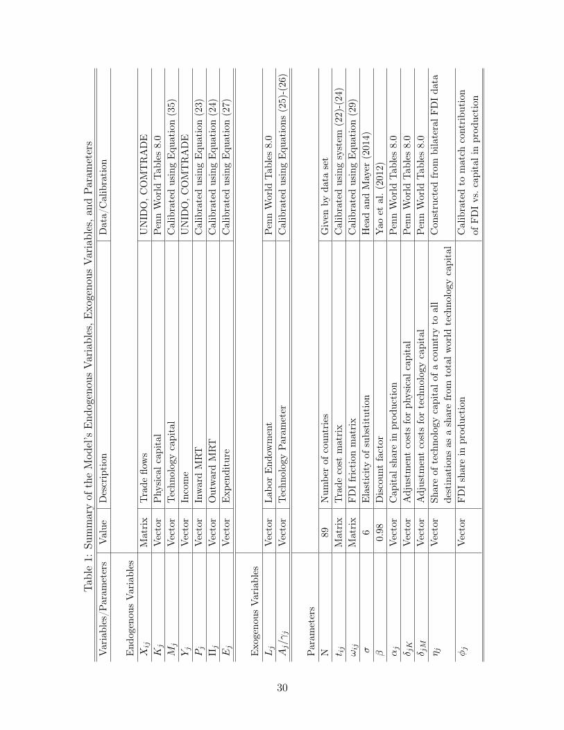
data are summarized in Table 1.

Data on employment and capital stocks are from the Penn World Tables (PWT) 8.0.14

The Penn World Tables 8.0 include data that enables us to measure employment in effective

units for all countries in our sample. To do this we multiply the Number of persons engaged in

the labor force with the Human capital index, which is based on average years of schooling.

Capital stocks in the Penn World Tables 8.0 are constructed based on accumulating and

depreciating past investments using the perpetual inventory method. For more detailed

information on the construction and the original sources for the PWT series see Feenstra et

al. (2013).

Aggregate trade data come from the United Nations Statistical Division (UNSD) Com-

modity Trade Statistics Database (COMTRADE). In order to construct internal aggregate

trade, which is needed for the counterfactual analysis, we used the ratio between aggregate

manufacturing in gross values and total exports of manufacturing goods in order to construct

garia (BGR), Canada (CAN), Chile (CHL), China (CHN), Colombia (COL), Croatia (HRV), Czech Republic(CZE), Cyprus (CYP), Denmark (DNK), Ecuador (ECU), Egypt (EGY), Estonia (EST), Finland (FIN),France (FRA), Germany (DEU), Ghana (GHA), Greece (GRC), Hong Kong (HKG), Hungary (HUN), In-dia (IND), Indonesia (IDN), Iran (IRN), Ireland (IRL), Israel (ISR), Italy (ITA), Japan (JPN), Kazakhstan(KAZ), Kenya (KEN), Korea, Republic of (KOR), Kuwait (KWT), Lebanon (LBN), Lithuania (LTU), Latvia(LVA), Luxembourg (LUX), Macedonia (MKD), Malaysia (MYS), Malta (MLT), Mexico (MEX), Morocco(MAR), Netherlands (NLD), New Zealand (NZL), Nigeria (NGA), Norway (NOR), Pakistan (PAK), Peru(PER), Philippines (PHL), Poland (POL), Portugal (PRT), Qatar (QAT), Romania (ROU), Russia (RUS),Saudi Arabia (SAU), Singapore (SGP), Slovak Republic (SVK), Slovenia (SVN), South Africa (ZAF), Spain(ESP), Sweden (SWE), Switzerland (CHE), Syria (SYR), Thailand (THA), Turkey (TUR), Ukraine (UKR),United Kingdom (GBR), United States (USA), Uzbekistan (UZB), Venezuela (VEN), and Vietnam (VNM).2011 was determined by the availability of capital stock data.

14These series are now maintained by the Groningen Growth and Development Centre and reside athttp://www.rug.nl/research/ggdc/data/pwt/. We refer the reader to Feenstra et al. (2013) for details onthe PWT dataset and we are very grateful to Robert Inklaar and Marcel Timmer for useful insights andclarifications regarding the PWT data.

17

a multiplier at the country-time level.15 We then used this multiplier along with data on ag-

gregate exports to project the values for intra-national trade. Data on gross manufacturing

production, which came from the United Nations’ IndStat database, enabled us to construct

multiplier indexes for half of the counties in our sample. We used a rest-of-the-world (ROW)

multiplier index to construct the rest of the internal trade data.

FDI data come from two sources. The main source is the newly constructed Bilateral

FDI Statistics database of the United Nations Conference on Trade and Development (UNC-

TAD).16 UNCTAD’s FDI data covers inflows, outflows, inward stock, and outward stock for

206 countries over the period 1990-2011. Data are collected from national sources and in-

ternational organizations. In order to ensure maximum coverage, mirror data from partner

countries is used as well. The second source of FDI data is the International Direct In-

vestment Statistics database, which is constructed and maintained by the Organization for

Economic Co-operation and Development (OECD).17 OECD’s data offers detailed statistics

for inward and outward foreign direct investment flows and positions (stocks) of the OECD

countries, including transactions between the OECD members and non-member countries.

We used the OECD data to ensure consistency and maximum coverage. Finally, we note that

the focus throughout the analysis is on FDI stocks (positions), which is the FDI category

for which most data are available and which is also the theoretically consistent measure.

The parameters needed to run counterfactuals with our model come from three sources.

Parameters borrowed from the literature include the elasticity of substitution (σ = 6), which15An alternative approach is to construct intra-national trade flows as the difference between GDP data,

which are widely available, and data on total exports. However this procedure is inconsistent with our theorybecause GDP is a measure of value added while total exports are a gross measure. Another alternative is touse the World Input-Output Database (WIOD) data, which includes consistently constructed intra-nationaltrade flows. The main disadvantage of the WIOD data is its limited country coverage (43 countries), whichwill prevent us from focusing on many of the developed countries, where we expect the impact of FDI to besignificant.

16UNCTAD’s Bilateral FDI Statistics database can be found and accessed from UNCTAD’s web siteat http://unctad.org/en/Pages/DIAE/FDI%20Statistics/FDI-Statistics-Bilateral.aspx. We are extremelygrateful to Marco Fugazza who answered many questions and offered useful insights about the FDI data.We also thank colleagues at Global Affairs Canada, and Felix Stips from the University of Bayreuth whohelped with the downloading and the formatting of earlier versions of the UNCTAD FDI data.

17We thank George Pinel from Drexel University for his help with the downloading and formatting of theOECD FDI data.

18

is about the average and very close to the preferred reported value by Head and Mayer

(2014);18 the consumer discount factor (β = 0.98), which is from Yao et al. (2012); the

country-specific capital shares of production (αj); and the country-specific adjustment costs

of capital (δj), which come from the Penn World Tables.19 The exact values for the α’s and

δ’s are reported in columns (2) and (3) of Table 2, respectively.

A second group of parameters are constructed directly from the data. To calculate ηi,

i.e., the share of technology capital of a country to all destinations as a share from total

world technology capital, we use the data on FDIvalueij and calculate ηi as follows:

ηi =

∑j FDI

valueij∑

i

∑j FDI

valueij

. (33)

In addition, we calculate the production share of FDI using the relationship between inward

FDI (FDI inj =∑

i FDIvalueij ) and physical capital in the production function along with FDI

and physical capital data and data on the capital shares:20

φj =αj × (FDI inj /Kj)

1 + αj(FDI inj /Kj). (34)

The values for η and φ are reported in columns (3) and (4) of Table 2.

The third group of parameters that we use are calibrated to fit the model. These parame-

ters include the bilateral trade frictions (tij), which are calibrated from Equations (22)-(24);

the FDI frictions (ωij), which are constructed from Equation (29); the preference adjusted

technology parameters (Aj/γj), which is calibrated using Equations (25) and (26); and the

endogenous values for technology capital, which are calibrated using the following theory-18Head and Mayer (2014) report elasticities of trade with respect to trade costs, which are given by 1− σ

in our framework. Hence, the reported average value of −4.51 translates to a σ of 5.51, while the preferredestimate based on tariff data of −5.03 implies σ = 6.03.

19Due to the lack of data, we use the same country-specific depreciation rates for physical and technologycapital.

20Specifically, we use that φjYj is the share of spending on inward FDI and (1 − φj)αjYj the share ofspending on capital, which also enables us to construct country-specific φ’s.

19

consistent equation for technology capital:

Mj =βφηj

1− β + βδM

EjPj

for all j. (35)

Finally, we construct the inward and the outward multilateral resistance indexes using Equa-

tions (23) and (24), respectively. In order to perfectly match the differences between the value

of domestic income and expenditure in the data, we define ψj ≡ Ej/(Yj + ηj

∑i∈Nji,t φiYi −

φjYj∑

i∈Nij,t ηi

)as an exogenous country-specific parameter that accounts for any residual

trade imbalances that are not due the payments to inward and outward FDI, which are

already captured in our theory. We then keep this exogenous part of the trade imbalances

([(ψj − 1)/ψj]Ej) constant in our counterfactual analysis, while the part due to payments to

inward and outward FDI endogenously adjusts.21

3.2 Empirical Findings

Armed with our structural system of trade and investment from Section 2 and with the

data and parameters from the previous subsection, we proceed in this section to perform

a counterfactual experiment that simulates the steady state equilibrium of a hypothetical

world economy without FDI. Mechanically, we start in a baseline scenario, where trade,

domestic investment, and FDI are all active channels and then we increase FDI frictions to

eliminate all FDI in the world, while still allowing for trade and domestic investment.

In order to keep the presentation and the discussion of our results manageable, we focus

only on two outcomes of the counterfactual analysis. Specifically, first, we investigate the

implications of FDI for international trade. Then, we quantify the impact of FDI on welfare,

i.e. ‘the gains from FDI’, which is a standard experiment with respect to trade policy in

the related empirical trade literature. Given the dynamic nature of our model, in order to

measure welfare we follow Lucas (1987) and we obtain the welfare indexes by calculating21Note that it is ensured that world trade imbalances are zero in the baseline and the counterfactual.

20

the constant fraction ζ of aggregate consumption that consumers would need to be paid in

the baseline case to give them the same utility they obtain from consumption stream in the

counterfactual (Ccj ). Specifically, we calculate:

∞∑t=0

βt ln(Ccj

)=

∞∑t=0

βt ln

[(1 +

ζ

100

)Cbj

]⇒

ζ =(exp

[ln(Ccj

)− ln

(Cbj

)]− 1)× 100. (36)

Our findings with respect to the trade and welfare effects are reported in Table 2. Focus

first on the trade effects of FDI. The changes in trade due to no FDI are in column (6) of

Table 2, revealing a very substantial impact on trade. On average, trade would have been

11% lower without FDI in the world. Second, the impact of FDI on international trade

is quite heterogeneous across the countries in our sample. The countries whose trade has

benefitted the most from FDI, i.e. the countries with the most negative trade indexes in

column (6), are Luxembourg with a decrease of total exports of 90% after the hypothetical

elimination of FDI, followed by Belgium with a decrease in exports of 61%, and Hong Kong

with a fall in exports of 57%. In contrast, there are countries such as Pakistan, China

and India, that actually see an increase in their total exports of more than 10% due to the

elimination of FDI in the world.

The variation in the net FDI position of the countries in our sample offers a clue about

the reason for the heterogeneous results regarding the relationship between FDI and trade.

Net export of FDI and export trade are substitutes in the cross-section. Figure 1 plots the

counterfactual change in total exports from the elimination of FDI against the net FDI

position of countries. The Figure shows a best fit line with negative slope in the plot of

trade change against net FDI. This regularity has a simple partial equilibrium intuition.

The general equilibrium forces of the model modify the intuition, leading further insight into

the scatter of data points, especially the outliers.

The partial equilibrium reasoning is based on the effects of FDI elimination on expendi-

21

tures. FDI net position directly signs the capital services account: net inward FDI implies

that Ej < Yj. Elimination of FDI, all else equal, implies that Ej moves to equal Yj, rising

for net inward FDI and falling for net outward FDI.

Now put this relationship to work on the shift in the exports of country i:

∑j 6=i

Xij = Yi∑j 6=i

EjY

(tij

ΠiPj

)1−σ

= Yi

[1− Ei

Y

(tii

ΠiPi

)1−σ]. (37)

The elimination of FDI implies, all else equal, that Ei rises for net inward FDI and thus i’s

export trade falls according to the rightmost equality in (37). For net outward FDI Ei falls,

hence exports rise. This is the pattern of Figure 1.

The negative slope is most pronounced in the steeply sloped data cluster around net

FDI =0 in Figure 1. In contrast, the outliers (China, USA, Japan and Belgium) dampen

the relationship and suggest general equilibrium forces at work. The modularity of the

model makes tracing the effect of FDI elimination straightforward. Essentially, countries

with negative net FDI lose global income share from FDI elimination (technology capital

is less profitable so less is accumulated) while countries with positive net FDI gain income

share (domestic technology capital accumulation becomes more profitable following the loss

of imported technology capital). Our simulation results strongly show this effect. By (37)

this effect on the right and left outliers flattens the best fit line in Figure 1.

A secondary general equilibrium effect is the effect of FDI elimination on multilateral

resistances. Our simulations show that net FDI is negatively associated with outward mul-

tilateral resistance Πi, with a scatter plot closely resembling Figure 1. Net FDI is positively

associated with inward multilateral resistance, but less strongly than the negative associa-

tion with outward multilateral resistance. All else equal, these multilateral resistance effects

in (37) would raise exports, so the full general equilibrium effect in Figure 1 arises because

the direct effects of FDI elimination on Ei and Yi discussed in the preceding two paragraphs

dominates.

22

Thus while general equilibrium forces of the model act to blur the negative association of

net FDI and trade changes, the direct link between expenditures and the net FDI position

predominates enough to explain the negative slope in Figure 1.

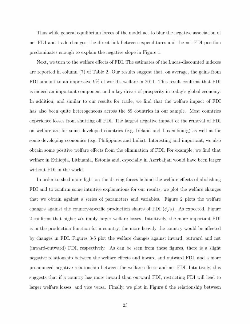
Next, we turn to the welfare effects of FDI. The estimates of the Lucas-discounted indexes

are reported in column (7) of Table 2. Our results suggest that, on average, the gains from

FDI amount to an impressive 9% of world’s welfare in 2011. This result confirms that FDI

is indeed an important component and a key driver of prosperity in today’s global economy.

In addition, and similar to our results for trade, we find that the welfare impact of FDI

has also been quite heterogeneous across the 89 countries in our sample. Most countries

experience losses from shutting off FDI. The largest negative impact of the removal of FDI

on welfare are for some developed countries (e.g. Ireland and Luxembourg) as well as for

some developing economies (e.g. Philippines and India). Interesting and important, we also

obtain some positive welfare effects from the elimination of FDI. For example, we find that

welfare in Ethiopia, Lithuania, Estonia and, especially in Azerbaijan would have been larger

without FDI in the world.

In order to shed more light on the driving forces behind the welfare effects of abolishing

FDI and to confirm some intuitive explanations for our results, we plot the welfare changes

that we obtain against a series of parameters and variables. Figure 2 plots the welfare

changes against the country-specific production shares of FDI (φj’s). As expected, Figure

2 confirms that higher φ’s imply larger welfare losses. Intuitively, the more important FDI

is in the production function for a country, the more heavily the country would be affected

by changes in FDI. Figures 3-5 plot the welfare changes against inward, outward and net

(inward-outward) FDI, respectively. As can be seen from these figures, there is a slight

negative relationship between the welfare effects and inward and outward FDI, and a more

pronounced negative relationship between the welfare effects and net FDI. Intuitively, this

suggests that if a country has more inward than outward FDI, restricting FDI will lead to

larger welfare losses, and vice versa. Finally, we plot in Figure 6 the relationship between

23

welfare and the change in total exports induced by restricting FDI. Smaller negative or larger

positive changes of trade lead to smaller welfare losses. Thus, the figure suggests that for

some countries, as Ethiopia, Pakistan and China, for example, restricting FDI leads to an

increase of total exports, mitigating the negative welfare effects from the removal of FDI.

In sum, the analysis in this section and the estimates from Table 2 reveal that FDI has

had significant but uneven impact on trade and welfare across the countries in the world.

Importantly, our estimates suggest that, while international trade and welfare in the world

on average and in most of the countries in our sample have been affected positively by FDI,

there are countries that have incurred losses due to FDI. In addition to pointing to the

specific need for those countries to re-evaluate their national policies toward FDI, our results

have implications for cross country inequality and for regional policies, which is of significant

policy interest, c.f. European Commission (2010). For example, according to our results,

some of the smaller and poorer nations in the European Union (including Cyprus, Bulgaria,

Ireland, and Malta) are among the countries that have enjoyed the largest positive impact

of FDI on both trade and welfare. This implies that FDI has lead to a decrease in income

inequality in Europe. In addition, we find that the majority of the countries that have lost

the most from FDI are former Soviet Union republics.

4 Conclusion

In this paper we developed a structural dynamic model that accounts for the economic impact

of foreign direct investment (FDI) in the global economy and decomposes the relationships

between trade, domestic investment via physical capital accumulation and FDI in the form

of non-rival technology capital. Our counterfactual experiment of characterizing a hypothet-

ical world without FDI demonstrated the effectiveness of our methods and the empirical

importance of FDI as a key component of the global economy with significant contributions

to welfare and inequality.

24

We see several possibilities to extend our analysis in new directions and to offer mean-

ingful additional contributions. First, since we were limited by FDI data availability, we did

not incorporate sectors in our model. In light of recent developments in the related trade

literature, e.g. Caliendo and Parro (2015), who demonstrate the importance of allowing for

input-output linkages, we expect that a sectoral model of trade and investment with interme-

diates will prove quantitatively important and will generate new insights about the impact

of FDI. Another possible direction for further research that is motivated by our analysis is

in the area of FDI estimations. Specifically, we expect that in combination with availability

of new reliable bilateral FDI data, the similarity between our structural FDI gravity system

and its popular trade counterpart will generate interest among researchers and policy makers

who are interested in studying the impact of various determinants of FDI.

25

References

Anderson, James E. and Eric van Wincoop, “Gravity with Gravitas: A Solution to

the Border Puzzle,” American Economic Review, 2003, 93 (1), 170–192.

and Yoto V. Yotov, “The Changing Incidence of Geography,” American Economic

Review, 2010, 100 (5), 2157–2186.

, Mario Larch, and Yoto V. Yotov, “Growth and Trade with Frictions: A Structural

Estimation Framework,” NBER Working Paper No. 21377, 2015.

Antras, Pol and Stephen R. Yeaple, “Multinational Firms and the Structure of In-

ternational Trade,” Vol. 4 of Handbook of International Economics, Chapter 0, 55-130.

Elsevier, 2014.

Arkolakis, Costas, Arnaud Costinot, and Andrés Rodríguez-Clare, “New Trade

Models, Same Old Gains?,” American Economic Review, 2012, 102 (1), 94–130.

Armington, Paul S., “A Theory of Demand for Products Distinguished by Place of Pro-

duction,” IMF Staff Papers, 1969, 16, 159–176.

Baldwin, Richard E. and Elena Seghezza, “Testing for Trade-Induced Invest- ment-Led

Growth,” International Economics, 2008, 61 (2-3), 507–537.

Bergstrand, Jeffrey H. and Peter H. Egger, “A Knowledge-and-Physical-Capital Model

of International Trade Flows, Foreign Direct Investment, and Multinational Enterprises,”

Journal of International Economics, 2007, 73 (2), 278–308.

and , “A General Equilibrium Theory for Estimating Gravity Equations of Bilateral

FDI, Final Goods Trade, and Intermediate Trade Flows,” in Peter A.G. van Bergeijk

and Steven Brakman, eds., The Gravity Model in International Trade – Advances and

Applications, Cambridge, United Kingdom: Cambridge University Press, 2010, pp. 29–70.

26

Blonigen, Bruce A. and Jeremy Piger, “Determinants of Foreign Direct Investment,”

Canadian Journal of Economics, August 2014, 47 (3), 775–812.

Caliendo, Lorenzo and Fernando Parro, “Estimates of the Trade and Welfare Effects

of NAFTA,” Review of Economic Studies, 2015, 82 (1), 1–44.

Costinot, Arnaud and Andrés Rodríguez-Clare, “Trade Theory with Numbers: Quan-

tifying the Consequences of Globalization,” Chapter 4 in the Handbook of International

Economics Vol. 4, eds. Gita Gopinath, Elhanan Helpman, and Kenneth S. Rogoff, Elsevier

Ltd., Oxford, 2014, pp. 197–261.

Cuñat, Alejandro and Marco Maffezzoli, “Can Comparative Advantage Explain the

Growth of US Trade?,” Economic Journal, 2007, 117 (520), 583–602.

Eaton, Jonathan, Samuel Kortum, Brent Neiman, and John Romalis, “Trade and

the Global Recession,” American Economic Review, 2016, 106 (11), 3401–3438.

Eicher, Theo S., Lindy Helfman, and Alex Lenkoski, “Robust FDI Determinants:

Bayesian Model Averaging in the Presence of Selection Bias,” Journal of Macroeconomics,

2012, 34 (3), 637–651.

European Commission, Investing in Europe’s Future, Editor: Eric von Breska, 2010.

Feenstra, Robert C., Robert Inklaar, and Marcel P. Timmer, “The Next Generation

of the Penn World Table,” available for download at http://www.ggdc.net/pwt, 2013.

Head, Keith and John Ries, “FDI as an Outcome of the Market for Corporate Control:

Theory and Evidence,” Journal of International Economics, 2008, 74 (1), 2–20.

Head, Keith and Thierry Mayer, “Gravity Equations: Workhorse, Toolkit, and Cook-

book,” Chapter 3 in the Handbook of International Economics Vol. 4, eds. Gita Gopinath,

Elhanan Helpman, and Kenneth S. Rogoff, Elsevier Ltd., Oxford, 2014, pp. 131–195.

27

Lucas, Robert E. Jr., Models of Business Cycles, New York: Basil Blackwell, 1987.

Markusen, James R., Multinational Firms and the Theory of International Trade, Cam-

bridge, Massachusetts: The MIT Press, 2002.

Markusen, J.R., “Trade versus Investment Liberalization,” NBER Working Paper No.

6231, 1997.

and K.E. Maskus, “Discriminating Among Alternative Theories of the Multinational

Enterprise,” Review of International Economics, 2002, 10 (4), 694–707.

McGrattan, Ellen R. and Andrea Waddle, “The Impact of Brexit on Foreign Investment

and Production,” NBER Working Paper No. 23217, 2017.

and Edward C. Prescott, “Openness, Technology Capital, and Development,” Journal

of Economic Theory, 2009, 144 (6), 2454–2476.

and , “Technology Capital and the US Current Account,” American Economic Review,

2010, 100 (4), 1493–1522.

McGrattan, Ellen R. and Edward C. Prescott, “A Reassessment of Real Business

Cycle Theory,” American Economic Review, 2014, 104 (5), 177–182.

OECD, “Cost Savings Stemming from Non-Compliance with International Environmental

Regulations in the Maritime Sector,” DSTI/DOT/MTC(2002)8/FINAL, http://www.oecd.

org/, 2002.

Olivero, María Pía and Yoto V. Yotov, “Dynamic Gravity: Endogenous Country Size

and Asset Accumulation,” Canadian Journal of Economics, 2012, 45 (1), 64–92.

Sampson, Thomas, “Dynamic Selection: An Idea Flows Theory of Entry, Trade, and

Growth,” The Quarterly Journal of Economics, 2016, 131 (1), 315–380.

28

Slaughter, Matthew J., “Attracting Foreign Direct Investment through an Ambitious

Trade Agenda,” Organization for International Investment Research Report, Washington,

D.C., 2013.

The World Bank, “Foreign Direct Investment and Development: Insights From Literature

and Ideas For Research,” http://blogs.worldbank.org/psd/foreign-direct-investment-and-

development-insights-literature-and-ideas-research, submitted by C. Qiang. Co-authors: R.

Echandi and J. Krajcovicova, 2015.

Wacziarg, Romain, “Measuring the Dynamic Gains from Trade,” World Bank Economic

Review, 2001, 15 (3), 393–425.

and Karen Horn Welch, “Trade Liberalization and Growth: New Evidence,” World

Bank Economic Review, 2008, 22 (2), 187–231.

Yao, S., C. F. Mela, J. Chiang, and Y. Chen, “Determining Consumers’ Discount

Rates with Field Studies,” Journal of Marketing Research, 2012, 49 (6), 822–841.

29

T able1:

Summaryof

theMod

el’s

End

ogenou

sVariables,E

xogeno

usVariables,a

ndParam

eters

Variables/P

aram

eters

Value

Description

Data/Calibratio n

End

ogenou

sVariables

Xij

Matrix

Trade

flows

UNID

O,C

OMTRADE

Kj

Vector

Phy

sicalc

apital

PennWorld

Tab

les8.0

Mj

Vector

Techn

ologycapital

CalibratedusingEqu

ation(35)

Yj

Vector

Income

UNID

O,C

OMTRADE

Pj

Vector

InwardMRT

CalibratedusingEqu

ation(23)

Πj

Vector

OutwardMRT

CalibratedusingEqu

ation(24)

Ej

Vector

Exp

enditure

CalibratedusingEqu

ation(27)

Exo

geno

usVariables

Lj

Vector

Labo

rEnd

owment

PennWorld

Tab

les8.0

Aj/γ

jVector

Techn

ologyParam

eter

CalibratedusingEqu

ations

(25)-(26)

Param

eters

N89

Num

berof

coun

tries

Given

byda

taset

t ij

Matrix

Trade

cost

matrix

Calibratedusingsystem

(22)-(24)

ωij

Matrix

FDIfriction

matrix

CalibratedusingEqu

ation(29)

σ6

Elasticityof

substitution

Headan

dMayer

(2014)

β0.98

Discoun

tfactor

Yao

etal.(

2012)

αj

Vector

Cap

ital

sharein

prod

uction

PennWorld

Tab

les8.0

δ jK

Vector

Adjustm

entcostsforph

ysical

capital

PennWorld

Tab

les8.0

δ jM

Vector

Adjustm

entcostsfortechno

logy

capital

PennWorld

Tab

les8.0

η jVector

Shareof

techno

logy

capitalo

facoun

tryto

all

Con

structed

from

bilateralF

DIda

tadestinations

asasharefrom

totalw

orld

techno

logy

capital

φj

Vector

FDIsharein

prod

uction

Calibratedto

match

contribu

tion

ofFDIvs.c

apital

inprod

uction

30

Table 2: Calibration Results and Results of Counterfactual Analysis

(1) (2) (3) (4) (5) (6) (7)

Country α δ η φ Trade Welfare

AGO 0.47 0.05 0.00 0.06 -20.25 -2.78

ARG 0.57 0.04 0.01 0.02 -5.35 -13.94

AUS 0.44 0.04 0.01 0.05 -21.38 -9.12

AUT 0.43 0.04 0.01 0.06 -12.91 -14.10

AZE 0.79 0.07 0.00 0.04 -16.05 5.61

BEL 0.38 0.05 0.01 0.24 -60.54 -12.50

BGD 0.47 0.04 0.00 0.00 4.12 -1.47

BGR 0.51 0.06 0.00 0.09 -17.22 -13.38

BLR 0.48 0.05 0.00 0.03 -4.76 -0.10

BRA 0.44 0.05 0.03 0.04 -8.76 -11.73

CAN 0.39 0.04 0.02 0.06 -12.99 -18.40

CHE 0.35 0.06 0.01 0.19 -42.87 -22.55

CHL 0.55 0.04 0.00 0.06 -13.40 -13.86

CHN 0.46 0.05 0.18 0.01 11.49 -11.77

COL 0.39 0.04 0.01 0.01 2.26 -3.68

CYP 0.48 0.04 0.00 0.19 -39.58 -32.51

CZE 0.49 0.04 0.00 0.06 -18.06 -1.98

DEU 0.39 0.04 0.04 0.03 -5.73 -7.69

DNK 0.37 0.04 0.00 0.05 -12.04 -12.35

DOM 0.34 0.03 0.00 0.01 -2.23 -0.95

ECU 0.55 0.05 0.00 0.01 -0.49 -1.38

EGY 0.62 0.06 0.00 0.03 -6.95 -9.44

ESP 0.39 0.04 0.02 0.05 -7.45 -13.31

EST 0.42 0.05 0.00 0.09 -24.93 0.07

ETH 0.47 0.05 0.00 0.00 8.37 0.30

FIN 0.39 0.04 0.00 0.05 -9.78 -7.72

FRA 0.37 0.04 0.03 0.04 -4.86 -10.61

GBR 0.39 0.04 0.03 0.08 -19.63 -17.16

GHA 0.47 0.06 0.00 0.02 -4.61 -3.08

GRC 0.47 0.03 0.00 0.01 2.54 -8.01

GTM 0.58 0.05 0.00 0.03 -9.98 -3.86

HKG 0.48 0.04 0.01 0.23 -57.24 -20.34

HRV 0.34 0.04 0.00 0.04 -8.26 -4.41

HUN 0.41 0.04 0.00 0.07 -12.73 -10.68

IDN 0.54 0.04 0.01 0.02 -3.30 -7.51

IND 0.50 0.06 0.04 0.01 10.76 -10.68

Continued on next page

31

Table 2 – Continued from previous page

(1) (2) (3) (4) (5) (6) (7)

Country α δ η φ Trade Welfare

IRL 0.52 0.05 0.00 0.29 -48.47 -54.89

IRN 0.74 0.06 0.01 0.00 3.38 -4.44

IRQ 0.70 0.06 0.00 0.00 -1.99 -1.18

ISR 0.45 0.04 0.00 0.03 -7.33 -8.87

ITA 0.46 0.04 0.03 0.02 -1.07 -8.89

JPN 0.39 0.05 0.07 0.00 9.53 -8.52

KAZ 0.58 0.04 0.00 0.06 -23.65 -7.65

KEN 0.57 0.05 0.00 0.02 -2.53 -2.46

KOR 0.50 0.05 0.02 0.01 0.40 -6.10

KWT 0.75 0.06 0.00 0.01 1.02 -7.07

LBN 0.56 0.04 0.00 0.00 7.28 -7.51

LKA 0.31 0.04 0.00 0.00 3.65 -2.47

LTU 0.53 0.04 0.00 0.06 -14.59 1.85

LUX 0.46 0.05 0.01 0.63 -89.80 -43.53

LVA 0.45 0.03 0.00 0.05 -14.03 -2.66

MAR 0.51 0.05 0.00 0.05 -8.96 -8.18

MEX 0.61 0.04 0.02 0.05 -11.05 -17.42

MKD 0.47 0.04 0.00 0.03 -6.14 -1.77

MLT 0.46 0.05 0.00 0.22 -32.55 -16.43

MYS 0.47 0.06 0.01 0.03 -7.47 -10.07

NGA 0.50 0.06 0.00 0.05 -19.69 -1.70

NLD 0.41 0.04 0.02 0.11 -16.98 -17.43

NOR 0.48 0.04 0.00 0.09 -23.38 -14.17

NZL 0.43 0.04 0.00 0.08 -26.59 -6.05

OMN 0.70 0.06 0.00 0.03 -10.65 -1.34

PAK 0.47 0.06 0.00 0.01 15.73 -9.54

PER 0.69 0.04 0.00 0.02 -5.06 -3.06

PHL 0.64 0.05 0.00 0.01 -2.03 -17.84

POL 0.44 0.05 0.01 0.05 -7.27 -8.81

PRT 0.39 0.04 0.00 0.04 -8.03 -11.80

QAT 0.81 0.10 0.00 0.03 -8.51 -12.50

ROM 0.53 0.05 0.00 0.05 -11.00 -9.85

RUS 0.26 0.04 0.03 0.01 5.80 -2.87

SAU 0.72 0.05 0.01 0.01 -0.94 -2.85

SDN 0.41 0.07 0.00 0.01 -4.07 -0.86

SER 0.42 0.04 0.00 0.03 -9.74 -1.42

SGP 0.56 0.05 0.00 0.18 -40.51 -23.60

Continued on next page

32

Table 2 – Continued from previous page

(1) (2) (3) (4) (5) (6) (7)

Country α δ η φ Trade Welfare

SVK 0.46 0.05 0.00 0.07 -21.45 1.65

SVN 0.33 0.04 0.00 0.02 -5.39 -0.11

SWE 0.45 0.05 0.00 0.18 -34.93 -22.49

SYR 0.47 0.06 0.00 0.00 -0.20 -0.99

THA 0.61 0.07 0.01 0.04 -5.61 -13.54

TKM 0.47 0.04 0.00 0.00 -4.38 -1.30

TUN 0.50 0.05 0.00 0.01 0.71 -4.35

TUR 0.56 0.06 0.01 0.04 -5.81 -6.11

TZA 0.57 0.04 0.00 0.03 -12.48 -2.18

UKR 0.44 0.03 0.01 0.01 -0.84 -2.52

USA 0.40 0.05 0.18 0.02 2.66 -7.11

UZB 0.47 0.03 0.00 0.00 -1.17 -0.19

VEN 0.63 0.04 0.00 0.02 -6.45 -3.25

VNM 0.47 0.05 0.01 0.01 -1.67 -0.77

ZAF 0.46 0.05 0.00 0.07 -23.66 -6.38

ZWE 0.44 0.04 0.00 0.08 -16.88 -0.47

Notes: This table reports results from our FDI coun-

terfactual. Column (1) lists the country abbreviations.

Columns (2) reports the calculated capital shares α. In

column (3) we report the calculated depriciation rates δ.

Column (4) gives the shares of technology capital of a

country to all destinations as a share from total world

technology capital η, while column (5) reports the pro-

duction shares of FDI φ. Column (6) and (7) report per-

centage changes in total exports and welfare for the FDI

counterfactual. See text for further details.

33

Figure 1: FDI Impact on Trade and the Net FDI Position.

AGO

ARG

AUSAUTAZE

BEL

BGD

BGR

BLRBRACAN

CHE

CHL

CHNCOL

CYP

CZE

DEUDNKDOMECUEGYESP

EST

ETH

FINFRA

GBR

GHAGRC

GTM

HKG

HRVHUN

IDN

IND

IRL

IRNIRQISR

ITA

JPN

KAZ

KENKORKWTLBNLKA

LTU

LUX

LVAMARMEXMKD

MLT

MYS

NGANLDNORNZL

OMN

PAK

PERPHLPOLPRTQATROM

RUSSAUSDNSER

SGP

SVK

SVN

SWE

SYRTHATKMTUNTURTZA

UKRUSA UZBVENVNM

ZAFZWE

-100

.00

-50.

000.

0050

.00

trade

cha

nge

(%)

-50000 0 50000net FDI

trade Fitted values

Notes: This figure plots the change in total exports in responseto the elimination of FDI in the world against net FDI position,i.e. inward FDI − outward FDI, in the baseline scenario. See textfor further details.

Figure 2: FDI Impact on Welfare and the Production Shares of FDI (φ).

AGO

ARGAUSAUT

AZE

BEL

BGD

BGR

BLR

BRA

CANCHE

CHLCHN

COL

CYP

CZE

DEUDNK

DOMECU

EGYESP

ESTETH

FINFRA

GBR

GHAGRC

GTM

HKG

HRV

HUNIDN

IND

IRL

IRNIRQ

ISRITAJPN KAZKEN

KORKWTLBNLKA

LTU

LUX

LVA

MAR

MEX

MKD

MLT

MYS

NGA

NLDNOR

NZLOMN

PAK

PER

PHL

POLPRTQATROM

RUSSAUSDNSER

SGP

SVKSVN

SWE

SYR

THA

TKMTUNTUR

TZAUKRUSA

UZBVEN

VNM

ZAF

ZWE

-60.

00-4

0.00

-20.

000.

0020

.00

wel

fare

cha

nge

(%)

0.00 0.10 0.20 0.30 0.40 0.50 0.60φ

welfare Fitted values

Notes: This figure plots the change in welfare in response to theelimination of FDI in the world against the FDI share in produc-tion (φ). See text for further details.

34

Figure 3: FDI Impact on Welfare and Inward FDI.

AGO

ARGAUS

AUT

AZE

BEL

BGD

BGR

BLR

BRA

CANCHE

CHL CHN

COL

CYP

CZE

DEUDNK

DOMECU

EGYESP

ESTETH

FINFRA

GBR

GHAGRCGTM

HKG

HRV

HUNIDNIND

IRL

IRNIRQ

ISR ITAJPNKAZKEN

KORKWTLBNLKA

LTU

LUX

LVA

MAR

MEX

MKD

MLT

MYS

NGA

NLDNOR

NZLOMN

PAK

PER

PHL

POLPRTQATROM

RUSSAUSDNSER

SGP

SVKSVN

SWE

SYR

THA

TKMTUNTURTZAUKR

USA

UZBVEN

VNM

ZAF

ZWE

-60.

00-4

0.00

-20.

000.

0020

.00

wel

fare

cha

nge

(%)

0 10000 20000 30000 40000 50000inward FDI

welfare Fitted values

Notes: This figure plots the change in welfare in response to theelimination of FDI in the world against inward FDI in the baseline.See text for further details.

Figure 4: FDI Impact on Welfare and Outward FDI.

AGO

ARGAUS

AUT

AZE

BEL

BGD

BGR

BLR

BRA

CANCHE

CHL CHN

COL

CYP

CZE

DEUDNK

DOMECU

EGYESP

ESTETH

FINFRA

GBR

GHAGRC

GTM

HKG

HRV

HUNIDN

IND

IRL

IRNIRQ

ISR ITA JPNKAZKEN

KORKWTLBNLKALTU

LUX

LVA

MAR

MEX

MKD

MLT

MYS

NGA

NLDNOR

NZLOMN

PAK

PER

PHL

POLPRTQAT

ROM

RUSSAUSDNSER

SGP

SVKSVN

SWE

SYR

THA

TKMTUNTURTZAUKR

USA

UZBVENVNM

ZAF

ZWE

-60.

00-4

0.00

-20.

000.

0020

.00

wel

fare

cha

nge

(%)

0 10000 20000 30000 40000 50000outward FDI

welfare Fitted values

Notes: This figure plots the change in welfare in response tothe elimination of FDI in the world against outward FDI in thebaseline. See text for further details.

35

Figure 5: FDI Impact on Welfare and Net FDI Position.

AGO

ARGAUS

AUT

AZE

BEL

BGD

BGR

BLR

BRA

CANCHE

CHLCHN

COL

CYP

CZE

DEUDNK

DOMECU

EGYESP

ESTETH

FINFRA

GBR

GHAGRCGTM

HKG

HRV

HUNIDN

IND

IRL

IRNIRQ

ISRITAJPN KAZKEN

KORKWTLBNLKALTU

LUX

LVA

MAR

MEX

MKD

MLT

MYS

NGA

NLDNOR

NZLOMN

PAK

PER

PHL

POLPRTQATROM

RUSSAUSDNSER

SGP

SVKSVN

SWE

SYR

THA

TKMTUNTURTZAUKR

USA

UZBVENVNM

ZAF

ZWE

-60.

00-4

0.00

-20.

000.

0020

.00

wel

fare

cha

nge

(%)

-50000 0 50000net FDI

welfare Fitted values

Notes: This figure plots the change in welfare in response to theelimination of FDI in the world against the net FDI position. Seetext for further details.

Figure 6: FDI Impact on Welfare and the Change in Total Exports.

AGO

ARGAUS

AUT

AZE

BEL

BGD

BGR

BLR

BRA

CANCHE

CHL CHN

COL

CYP

CZE

DEUDNK

DOMECU

EGYESP

EST ETH

FINFRA

GBR

GHAGRC

GTM

HKG

HRV

HUNIDN

IND

IRL

IRNIRQ

ISR ITA JPNKAZKEN

KORKWTLBNLKA

LTU

LUX

LVA

MAR

MEX

MKD

MLT

MYS

NGA

NLDNOR

NZLOMN

PAK

PER

PHL

POLPRTQAT

ROM

RUSSAUSDNSER

SGP

SVK SVN

SWE

SYR

THA

TKMTUNTUR

TZA UKRUSA

UZBVEN

VNM

ZAF

ZWE

-60.

00-4

0.00

-20.

000.

0020

.00

wel

fare

cha

nge

(%)

-100.00 -80.00 -60.00 -40.00 -20.00 0.00 20.00trade change (%)

welfare Fitted values

Notes: This figure plots the change in welfare in response to theelimination of FDI in the world against the change in exports. Seetext for further details.

36

Appendix

A Derivation of System of Equations (22)-(29)

This appendix gives derivation details for our system of equations (22)-(29).

First, let us re-state our production function as given in Equation (1):

Yj,t = pj,tAj,t(L1−αj,t Kα

j,t

)1−φ(

N∏i=1

(max1, ωij,tMi,t)ηi)φ

α, φ ∈ (0, 1). (A1)

Note that we can write max1, ωij,tMi,t = (1 +ωij,tMi,t + |1−ωij,tMi,t|)/2 = (1 +ωij,tMi,t +

((1 − ωij,tMi,t)2)1/2)/2 .22 The derivative of max1, ωij,tMi,t with respect to Mi,t is given

by:23

(ωij,t −

(1− ωij,tMi,t)

((1− ωij,tMi,t)2)1/2ωij,t

)/2

=

(1− (1− ωij,tMi,t)

|1− ωij,tMi,t|

)ωij,t/2. (A2)

Using this definition of nominal output, the value marginal product of technology capital at

home is given by:

∂Yj,t∂Mj,t

=φηjYj,t

max1, ωjj,tMj,t

(1− (1− ωjj,tMj,t)

|1− ωjj,tMj,t|

)ωjj,t

2, (A3)

and the value marginal product of Mj,t abroad by:

∂Yi,t∂Mj,t

=φηjYi,t

max1, ωji,tMj,t

(1− (1− ωji,tMj,t)

|1− ωji,tMj,t|

)ωji,t

2. (A4)

Note that an alternative way of writing these two conditions is the following:22See for example https://math.stackexchange.com/questions/1633071/absolute-value-and-max-min-func

tion-why-a-b-a-b-2-maxa-b.23See for example http://organicchemist.us/organichem/my_pagesabsvalder.html.

A1

∂Yj,t∂Mj,t

=

φηjYj,tMj,t

if ωjj,tMj,t > 1,

0 if ωjj,tMj,t ≤ 1.

∂Yi,t∂Mj,t

=

φηjYi,tMj,t

if ωji,tMj,t > 1,

0 if ωji,tMj,t ≤ 1.

With this new expressions for the value marginal products, disposable income can be written

as:

Ej,t = Yj,t + φηjMj,t

∑i6=j

Yi,tmax1, ωji,tMj,t

(1− (1− ωji,tMj,t)

|1− ωji,tMj,t|

)ωji,t

2(A5)

− φYj,t∑i6=j

ηiMi,t

max1, ωij,tMi,t

(1− (1− ωij,tMi,t)

|1− ωij,tMi,t|

)ωij,t

2,

which describes expenditure as the sum of total nominal output (Yj,t) plus rents from foreign

investments (∑

i6=jMj,t × ∂Yi,t∂Mj,t

), minus rents accruing to foreign investments (∑

i6=jMi,t ×∂Yj,t∂Mi,t

), which are part of nominal output. Rewriting a bit further, we end up with:

Ej,t = Yj,t + φηj∑i 6= j,

ωji,tMj,t > 1

Yi,t − φYj,t∑i 6= j,

ωij,tMi,t > 1

ηi. (A6)

In the next subsection, we first derive the solution of the dynamic problem. Afterward, we

state the steady-state of the system.

A.1 Solving the ‘Upper Level’

This section details the Lagrangian problem and the corresponding first-order conditions for

the ‘upper level’ optimization problem leading to the structural dynamic system of trade,

growth, and FDI.

A2

We assume a log-intertemporal utility function:

Uj,t =∞∑t=0

βt ln(Cj,t), (A7)

and combine the budget constraint given by Equation (16) with the expenditure function

given by Equation (A6):

Pj,tCj,t + Pj,tΩj,t + Pj,tχj,t = Yj,t + φηj∑i 6= j,

ωji,tMj,t > 1

Yi,t − φYj,t∑i 6= j,

ωij,tMi,t > 1

ηi

=

1− φ

∑i 6= j,

ωij,tMi,t > 1

ηi

Yj,t + φηj

∑i 6= j,

ωji,tMj,t > 1

Yi,t.

Further, we replace Yj,t with the production function as formulated in Equation (A1), leading

A3

to:

Pj,tCj,t + Pj,tΩj,t + Pj,tχj,t =1− φ

∑i 6= j,

ωij,tMi,t > 1

ηi

pj,tAj,t

(L1−αj,t Kα

j,t

)1−φ(

N∏i=1

(max1, ωij,tMi,t)ηi)φ

+φηj∑i 6= j,

ωji,tMj,t > 1

pi,tAi,t(L1−αi,t Kα

i,t

)1−φ(

N∏k=1

(max1, ωki,tMk,t)ηk)φ

.

In order to end up with only one constraint, we also replace Ωj,t and χj,t by using:

Ωj,t = Kj,t+1 − (1− δK)Kj,t,

χj,t = Mj,t+1 − (1− δM)Mj,t,

leading to the following budget constraint:

Pj,tCj,t + Pj,t (Kj,t+1 − (1− δK)Kj,t) + Pj,t (Mj,t+1 − (1− δM)Mj,t) =

(1− φ∑i 6= j,

ωij,tMi,t > 1

ηi)pj,tAj,t(L1−αj,t Kα

j,t

)1−φ(

N∏i=1

(max1, ωij,tMi,t)ηi)φ

+φηj∑i 6= j,

ωji,tMj,t > 1

pi,tAi,t(L1−αi,t Kα

i,t

)1−φ(

N∏k=1

(max1, ωki,tMk,t)ηk)φ

.

A4

The corresponding expression for the Lagrangian is:

Lj =∞∑t=0

βt[

ln(Cj,t) + λj,t

((1− φ

∑i 6= j,

ωij,tMi,t > 1

ηi)pj,tAj,t(L1−αj,t Kα

j,t

)1−φ

×

(N∏i=1

(max1, ωij,tMi,t)ηi)φ

+φηj∑i 6= j,

ωji,tMj,t > 1

pi,tAi,t(L1−αi,t Kα

i,t

)1−φ(

N∏k=1

(max1, ωki,tMk,t)ηk)φ

−Pj,tCj,t − Pj,t (Kj,t+1 − (1− δK)Kj,t)− Pj,t (Mj,t+1 − (1− δM)Mj,t))].

Take derivatives with respect to Cj,t, Kj,t+1 , Mj,t+1 and λj,t to obtain the following set of

first-order conditions:

∂Lj∂Cj,t

=βt

Cj,t− βtλj,tPj,t

!= 0 for all j and t. (A8)

∂Lj∂Kj,t+1

= βt+1λj,t+1(1− φ∑i 6= j,

ωij,t+1Mi,t+1 > 1

ηi)(1− φ)αYj,t+1

Kj,t+1

−βtλj,tPj,t

+βt+1λj,t+1Pj,t+1 (1− δK)!

= 0 for all j and t. (A9)

A5

∂Lj∂Mj,t+1

= βt+1λj,t+1(1− φ∑i 6= j,

ωij,t+1Mi,t+1 > 1

ηi)φηjYj,t+1

max1, ωjj,t+1Mj,t+1

×(

1− (1− ωjj,t+1Mj,t+1)

|1− ωjj,t+1Mj,t+1|

)ωjj,t+1

2(A10)

+ βt+1λj,t+1φηj

×∑i 6= j,

ωji,t+1Mj,t+1 > 1

φηjYi,t+1

max1, ωji,t+1Mj,t+1

(1− (1− ωji,t+1Mj,t+1)

|1− ωji,t+1Mj,t+1|

)ωji,t+1

2

(A11)

− βtλj,tPj,t

+ βt+1λj,t+1Pj,t+1 (1− δM)!

= 0 for all j and t. (A12)

∂Lj∂λj,t

= (1− φ∑i 6= j,

ωij,tMi,t > 1

ηi)pj,tAj,t(L1−αj,t Kα

j,t

)1−φ(

N∏i=1

(max1, ωij,tMi,t)ηi)φ

+φηj∑i 6= j,

ωji,tMj,t > 1

pi,tAi,t(L1−αi,t Kα

i,t

)1−φ(

N∏k=1

(max1, ωki,tMk,t)ηk)φ

−Pj,tCj,t − Pj,t (Kj,t+1 − (1− δK)Kj,t)− Pj,t (Mj,t+1 − (1− δM)Mj,t)

!= 0 for all j and t. (A13)

Use the first-order condition for consumption to express λj,t as:

λj,t =1

Cj,tPj,t. (A14)

A6

Replace this in the first-order condition for physical capital:

∂Lj∂Kj,t+1

= βt+1 1

Cj,t+1Pj,t+1

(1− φ∑i 6= j,

ωij,t+1Mi,t+1 > 1

ηi)(1− φ)αYj,t+1

Kj,t+1

−βt Pj,tCj,tPj,t

+βt+1 Pj,t+1

Cj,t+1Pj,t+1

(1− δK)!

= 0 for all j and t. (A15)

Simplify and re-arrange to obtain:

β(1− φ∑i 6= j,

ωij,t+1Mi,t+1 > 1

ηi)α(1− φ)Yj,t+1

Kj,t+1

− Cj,t+1Pj,t+1

Cj,t=

−β (1− δK)Pj,t+1 for all j and t. (A16)

Now replace λj with the expression from the first-order condition for consumption given in

A7

Equation (A14) in the first-order condition for technology capital given in Equation (A12):

∂Lj∂Mj,t+1

= βt+1 1

Cj,t+1Pj,t+1

(1− φ∑i 6= j,

ωij,t+1Mi,t+1 > 1

ηi)

× φηjYj,t+1

max1, ωjj,t+1Mj,t+1

(1− (1− ωjj,t+1Mj,t+1)

|1− ωjj,t+1Mj,t+1|

)ωjj,t+1

2

+βt+1 1

Cj,t+1Pj,t+1

φηj

×∑i 6= j,

ωji,t+1Mj,t+1 > 1

φηjYi,t+1

max1, ωji,t+1Mj,t+1

(1− (1− ωji,t+1Mj,t+1)

|1− ωji,t+1Mj,t+1|

)ωji,t+1

2

−βt 1

Cj,t

+βt+1

Cj,t+1

(1− δM)!

= 0 for all j and t. (A17)

Simplify and re-arrange to obtain:

β(1− φ∑i 6= j,

ωij,t+1Mi,t+1 > 1

ηi)φηjYj,t+1

max1, ωjj,t+1Mj,t+1

(1− (1− ωjj,t+1Mj,t+1)

|1− ωjj,t+1Mj,t+1|

)ωjj,t+1

2

+βφηj∑i 6= j,

ωji,t+1Mj,t+1 > 1

φηjYi,t+1

max1, ωji,t+1Mj,t+1

(1− (1− ωji,t+1Mj,t+1)

|1− ωji,t+1Mj,t+1|

)ωji,t+1

2

−Cj,t+1Pj,t+1

Cj,t=

β (1− δM)Pj,t+1 for all j and t. (A18)

Assuming that for sure ωjj,t+1Mj,t+1 > 1, i.e., technology stock at home is positive and

frictions small, we may simplify as follows:

A8

β(1− φ∑i 6= j,

ωij,t+1Mi,t+1 > 1

ηi)φηjYj,t+1

Mj,t+1

+ βφηj∑i 6= j,

ωji,t+1Mj,t+1 > 1

φηjYi,t+1

Mj,t+1

−Cj,t+1Pj,t+1

Cj,t=

−β (1− δM)Pj,t+1 for all j and t. (A19)

Combining the production function given by Equation (A1), the budget constraint given

by Equation (16), the expression for Ej,t given in Equation (A6), the expressions for pj,t

for each t from Equation (25), and the equations for the trade MRTs Pj,t and Πj,t given

by Equations (20) and (21), respectively, with the two first order conditions for Kj,t+1 and

Mj,t+1 as given by Equations (A16) and (A18), respectively, we end up with the following

A9

system:

Yj,t = pj,tAj,t(L1−αj,t Kα

j,t

)1−φ(

N∏i=1

(max1, ωij,tMi,t)ηi)φ

for all j and t, (A20)

Ej,t = Pj,tCj,t + Pj,t (Kj,t+1 − (1− δK)Kj,t)

+Pj,t (Mj,t+1 − (1− δM)Mj,t) for all j and t, (A21)

Ej,t = Yj,t + φηj∑i 6= j,

ωji,tMj,t > 1

Yi,t − φYj,t∑i 6= j,

ωij,tMi,t > 1

ηi for all j and t, (A22)

pj,t =(Yj,t/Yt)

11−σ

γjΠj,t

for all j and t, (A23)

Yt =N∑j=1

Yj,t for all t, (A24)

P 1−σj,t =

N∑i=1

(tij,tΠi,t

)1−σYi,tYt

for all j and t, (A25)

Π1−σi,t =

N∑j=1

(tij,tPj,t

)1−σEj,tYt

for all i and t, (A26)

β(1− φ∑i 6= j,

ωij,t+1Mi,t+1 > 1

ηi)α(1− φ)Yj,t+1

Kj,t+1

− Cj,t+1Pj,t+1

Cj,t=

β (δK − 1)Pj,t+1 for all j and t. (A27)

β(1− φ∑i 6= j,

ωij,t+1Mi,t+1 > 1

ηi)φηjYj,t+1

Mj,t+1

+ βφηj∑i 6= j,

ωji,t+1Mj,t+1 > 1

φηjYi,t+1

Mj,t+1

−Cj,t+1Pj,t+1

Cj,t= β (δM − 1)Pj,t+1 for all j and t. (A28)

This is a system of (8 ×N + 1) × T equations in the (8 ×N + 1) × T unknowns Cj,t, Kj,t,

A10

Mj,t, Yj,t, Yt, pj,t, Pj,t, Πj,t, Ej,t and given parameters and exogenous variables Aj,t, ωij,t, Lj,t,

α, β, φ, ηj, γj, σ, tij,t, δK , and δM .

A.2 Derivation of the Steady-State

In steady-state, values for t+ 1 and t have to be equal. Hence, we can express physical and

technology capital as:

Kj =Ωj

δK, (A29)

Mj =χjδM

. (A30)

Further, we can drop the time index for all variables. Let us first drop time indices and use

Kj = Ωj/δK and Mj = χj/δM in the first-order condition for physical capital as given in

Equation (A27):

β(1− φ∑i 6= j,

ωij,t+1Mi,t+1 > 1

ηi)α(1− φ)YjKj

− CjPjCj

=

β (δK − 1)Pj for all j.⇒

β(1− φ∑i 6= j,

ωij,t+1Mi,t+1 > 1

ηi)α(1− φ)YjPjKj

− 1 =

β (δK − 1) for all j.⇒

β(1− φ∑i 6= j,

ωij,t+1Mi,t+1 > 1

ηi)α(1− φ)/(1− β + βδK)YjPj

=

Kj for all j.

A11

Let us next drop time indices and use Kj = Ωj and Mj = χj in the first-order condition for

technology capital as given in Equation (A28):

β(1− φ∑i 6= j,

ωijMi > 1

ηi)φηjYjMj

+ βφηj∑i 6= j,

ωjiMj > 1

φηjYiMj

− CjPjCj

=

β (δM − 1)Pj for all j ⇒

β(1− φ∑i 6= j,

ωijMi > 1

ηi)φηjYjPjMj

+ βφηj∑i 6= j,

ωjiMj > 1

φηjYiPjMj

− 1 =

β (δM − 1) for all j ⇒βφηj

1− β + βδM((1− φ

∑i 6= j,

ωijMi > 1

ηi)YjPj

+∑i 6= j,

ωjiMj > 1

φηjYiPj

) =

Mj for all j ⇒βφηj

1− β + βδM

EjPj

=

Mj for all j ⇒

A12

Hence, the equation system given by Equations (A20)-(A28) simplifies to:

Yj = pjAj(L1−αj Kα

j

)1−φ(

N∏i=1

(max1, ωijMi)ηi)φ

for all j, (A31)

Ej = PjCj + PjKj + PjMj for all j, (A32)

Ej = Yj + φηj∑i 6= j,

ωjiMj > 1

Yi − φYj∑i 6= j,

ωijMi > 1

ηi for all j, (A33)

pj =(Yj/Y )

11−σ

γjΠj

for all j, (A34)

Y =N∑j=1

Yj, (A35)

P 1−σj =

N∑i=1

(tijΠi

)1−σYiY

for all j, (A36)

Π1−σi =

N∑j=1

(tijPj

)1−σEjY

for all i, (A37)

Kj = β(1− φ∑i 6= j,

ωij,t+1Mi,t+1 > 1

ηi)α(1− φ)/(1− β + βδK)YjPj

for all j, (A38)

Mj =βφηj

1− β + βδM

EjPj

for all j. (A39)

Note that trade flows in steady-state are then given by Xij =YiEjY

(tij

ΠiPj

)1−σ.

The steady state system above yields a convenient gravity representation of FDI that is

remarkably similar to the familiar trade gravity system. To obtain it, recall the (steady-state)

definition of bilateral FDI stock:

FDIij ≡ ωijMi. (A40)

A13

Use the steady-state solution for technology capital Mj from Equation (A39):

Mj =βφηj

1− β + βδM

EjPj. (A41)

Substitute for Mj in Equation (A40) to obtain:

FDIij = ωijβφηi

1− β + βδM

EiPi. (A42)

Equation (A42) resembles a gravity equation, except that it describes physical FDI stocks.

To translate (A42) into a stock value FDI equation needed for estimation with data on FDI

stock values, define the value of FDI from country i to country j as the product of the FDI

stock times its value marginal product:

FDIvalueij ≡ FDIij ×∂Yj∂Mi

(A43)

= ωijβφηi

1− β + βδM

EiPiφηi

YjMi

(A44)

=βφ2η2

i

1− β + βδMωij

EiPi

YjMi

. (A45)

Combine Equation (A42) with the definitions of the multilateral resistance terms Pj and Πj

given by Equations (20) and (21), respectively, to obtain the following FDI gravity system:

FDIvalueij =βφ2η2

i

1− β + βδMωij

EiPi

YjMi

, (A46)

Pi =

[N∑j=1

(tjiΠj

)1−σYjY

] 11−σ

, (A47)

Πj =

[N∑i=1

(tjiPi

)1−σEiY

] 11−σ

. (A48)

A14

B Sum as Functional Form for FDI Aggregation

Our production function as given in Equation (1) combined technology capital across all

countries of the world via a max-Cobb-Douglas function. The original formulation by Mc-

Grattan and Prescott (2009, 2010) summed over all technology capital stock. In this section,

we will explore the implications of this alternative specification.

Specifically, the production function is now assumed to be given by:

Yj,t = pj,tAj,t(L1−αj,t Kα

j,t

)1−φ(

N∑i=1

ωij,tMi,t

)φ

α, φ ∈ (0, 1). (A49)

Using this definition of nominal output, the value marginal product of technology capital at

home is given by:

∂Yj,t∂Mj,t

= φωjj,tYj,t∑N

i=1 ωij,tMi,t

, (A50)

and the value marginal product of Mj,t abroad by:

∂Yi,t∂Mj,t

= φωji,tYi,t∑N

k=1 ωki,tMk,t

. (A51)

With this new expressions for the value marginal products, disposable income reads as fol-

lows:

Ej,t = Yj,t + φMj,t

∑i6=j

(ωji,tYi,t∑N

k=1 ωki,tMk,t

)− φ Yj,t∑N

k=1 ωkj,tMk,t

∑i6=j

ωij,tMi,t, (A52)

which describes expenditure as the sum of total nominal output (Yj,t) plus rents from foreign

investments (∑

i6=jMj,t × ∂Yi,t∂Mj,t

=∑

i6=jMj,tφωji,tYi,t∑N

k=1 ωki,tMk,t= φMj,t

∑i6=j(

ωji,tYi,t∑Nk=1 ωki,tMk,t

)),

minus rents accruing to foreign investments (∑

i6=jMi,t× ∂Yj,t∂Mi,t

=∑

i6=jMi,tφωij,tYj,t∑N

k=1 ωkj,tMk,t

= φYj,t∑N

k=1 ωkj,tMk,t

∑i6=j ωij,tMi,t), which are part of nominal output.

All other assumptions are unchanged.

A15

B.1 First-Order Conditions

The next step is to look at the Lagrangian and the corresponding first-order conditions.

Specifically, we again assume a log-linear intertemporal utility function:

Uj,t =∞∑t=0

βt ln(Cj,t),

and combine the budget constraint given by Equation (16) (not replacing investment) with

the expenditure function given by Equation (A52):

Pj,tCj,t + Pj,tΩj,t + Pj,tχj,t = Yj,t

(1− φ∑N

k=1 ωkj,tMk,t

∑i6=j

ωij,tMi,t

)

+ φMj,t

∑i6=j

(ωji,tYi,t∑N

k=1 ωki,tMk,t

).

Further, we replace Yj,t with the production function as formulated in Equation (A49),

leading to:

Pj,tCj,t + Pj,tΩj,t + Pj,tχj,t = pj,tAj,t(L1−αj,t Kα

j,t

)1−φ(

N∑i=1

ωij,tMi,t

)φ

×(1− φ∑N

k=1 ωkj,tMk,t

∑i6=j

ωij,tMi,t

)

+ φMj,t

∑i6=j

ωji,tpi,tAi,t(L1−αi,t Kα

i,t

)1−φ(∑N

k=1 ωki,tMk,t

)φ∑N

k=1 ωki,tMk,t

.

In order to end up with only one constraint, we also replace Ωj,t and χj,t by:

Ωj,t = Kj,t+1 − (1− δK)Kj,t,

χj,t = Mj,t+1 − (1− δM)Mj,t,

A16

leading to the following budget constraint:

Pj,tCj,t + Pj,t (Kj,t+1 − (1− δK)Kj,t) + Pj,t (Mj,t+1 − (1− δM)Mj,t) =

pj,tAj,t(L1−αj,t Kα

j,t

)1−φ(

N∑i=1

ωij,tMi,t

)φ

×(1− φ∑N

k=1 ωkj,tMk,t

∑i6=j

ωij,tMi,t

)

+φMj,t

∑i6=j

ωji,tpi,tAi,t(L1−αi,t Kα

i,t

)1−φ(∑N

k=1 ωki,tMk,t

)φ∑N

k=1 ωki,tMk,t

.

The corresponding expression for the Lagrangian is:

Lj =∞∑t=0

βt[

ln(Cj,t) + λj,t

(pj,tAj,t

(L1−αj,t Kα

j,t

)1−φ(

N∑i=1

ωij,tMi,t

)φ

×

(1− φ∑N

k=1 ωkj,tMk,t

∑i6=j

ωij,tMi,t

)

+φMj,t

∑i6=j

ωji,tpi,tAi,t(L1−αi,t Kα

i,t

)1−φ(∑N

k=1 ωki,tMk,t

)φ∑N

k=1 ωki,tMk,t

−Pj,tCj,t − Pj,t (Kj,t+1 − (1− δK)Kj,t)− Pj,t (Mj,t+1 − (1− δM)Mj,t)

)].

A17

Take derivatives with respect to Cj,t, Kj,t+1 , Mj,t+1 and λj,t to obtain the following set of

first-order conditions:

∂Lj∂Cj,t

=βt

Cj,t− βtλj,tPj,t

!= 0 for all j and t. (A53)

∂Lj∂Kj,t+1

= βt+1λj,t+1pj,t+1Aj,t+1

(N∑i=1

ωij,t+1Mi,t+1

)φ

(1− φ∑N

k=1 ωkj,t+1Mk,t+1

∑i6=j

ωij,t+1Mi,t+1

)L

(1−α)(1−φ)j,t+1 α(1− φ)K

α(1−φ)−1j,t+1

−βtλj,tPj,t

+βt+1λj,t+1 (1− δK)Pj,t+1!

= 0 for all j and t. (A54)

A18

∂Lj∂Mj,t+1

= βt+1λj,t+1ωjj,t+1pj,t+1Aj,t+1

(L1−αj,t+1K

αj,t+1

)1−φφ(

1− φ∑Nk=1 ωkj,t+1Mk,t+1

∑i6=j

ωij,t+1Mi,t+1

)(N∑i=1

ωij,t+1Mi,t+1

)φ−1

+ βt+1λj,t+1ωjj,t+1pj,t+1Aj,t+1

(L1−αj,t+1K

αj,t+1

)1−φ(

N∑i=1

ωij,t+1Mi,t+1

)φ

×

φ(∑Nk=1 ωkj,t+1Mk,t+1

)2

∑i6=j

ωij,t+1Mi,t+1

+ βt+1λj,t+1φ

∑i6=j

ωji,t+1pi,t+1Ai,t+1

(L1−αi,t+1K

αi,t+1

)1−φ(∑N

k=1 ωki,t+1Mk,t+1

)φ∑N

k=1 ωki,t+1Mk,t+1

+ βt+1λj,t+1φMj,t+1

×∑i6=j

(ω2ji,t+1pi,t+1Ai,t+1

(L1−αi,t+1K

αi,t+1

)1−φφ(∑N

k=1 ωki,t+1Mk,t+1

)φ−1

∑Nk=1 ωki,t+1Mk,t+1

−ω2ji,t+1pi,t+1Ai,t+1

(L1−αi,t+1K

αi,t+1

)1−φ(∑N

k=1 ωki,t+1Mk,t+1

)φ(∑N

k=1 ωki,t+1Mk,t+1

)2

)(A55)

− βtλj,tPj,t

+ βt+1λj,t+1 (1− δM)Pj,t+1!

= 0 for all j and t. (A56)

∂Lj∂λj,t

= pj,tAj,t

(N∑i=1

ωij,tMi,t

)φ (L1−αj,t Kα

j,t

)1−φ

×

(1− φ∑N

k=1 ωkj,tMk,t

N∑i=1

ωij,tMi,t

)+ φMj,t

∑i6=j

(ωji,tYi,t∑N

k=1 ωki,tMk,t

)−Pj,tCj,t − Pj,t (Kj,t+1 − (1− δK)Kj,t)

−Pj,t (Mj,t+1 − (1− δM)Mj,t)!

= 0 for all j and t. (A57)

A19

Use the first-order condition for consumption to express λj,t as:

λj,t =1

Cj,tPj,t. (A58)

Replace this in the first-order condition for physical capital:

∂Lj∂Kj,t+1

= βt+1 1

Cj,t+1Pj,t+1

pj,t+1Aj,t+1

(N∑i=1

ωij,t+1Mi,t+1

)φ

(1− φ∑N

k=1 ωkj,t+1Mk,t+1

∑i6=j

ωij,t+1Mi,t+1

)L

(1−α)(1−φ)j,t+1 α(1− φ)K

α(1−φ)−1j,t+1

−βt 1

Cj,tPj,tPj,t

+βt+1 (1− δK)1

Cj,t+1Pj,t+1

Pj,t+1!

= 0 for all j and t. (A59)

Simplify and re-arrange to obtain:

β1

Cj,t+1Pj,t+1

pj,t+1Aj,t+1

(N∑i=1

ωij,t+1Mi,t+1

)φ

(1− φ∑N

k=1 ωkj,t+1Mk,t+1

∑i6=j

ωij,t+1Mi,t+1

)L

(1−α)(1−φ)j,t+1 α(1− φ)K

α(1−φ)−1j,t+1 =

1

Cj,t+

(δK − 1) β

Cj,t+1

for all j and t. (A60)

Use the definition of Yt to re-write the left-hand side of the above expression as:

α(1− φ)βYj,t+1

Kj,t+1Cj,t+1Pj,t+1

(1− φ∑N

k=1 ωkj,t+1Mk,t+1

∑i6=j

ωij,t+1Mi,t+1

)=

1

Cj,t+β (δK − 1)

Cj,t+1

for all j and t. (A61)

Now replace λj with the expression from the first-order condition for consumption given in

Equation (A58) in the first-order condition for technology capital given in Equation (A56):

A20

∂Lj∂Mj,t+1

= βt+1 1

Cj,t+1Pj,t+1

ωjj,t+1pj,t+1Aj,t+1

(L1−αj,t+1K

αj,t+1

)1−φφ(

1− φ∑Nk=1 ωkj,t+1Mk,t+1

∑i6=j

ωij,t+1Mi,t+1

)(N∑i=1

ωij,t+1Mi,t+1

)φ−1

+βt+1 1

Cj,t+1Pj,t+1

ωjj,t+1pj,t+1Aj,t+1

(L1−αj,t+1K

αj,t+1

)1−φ(

N∑i=1

ωij,t+1Mi,t+1

)φ

×

φ(∑Nk=1 ωkj,t+1Mk,t+1

)2

∑i6=j

ωij,t+1Mi,t+1

+βt+1 1

Cj,t+1Pj,t+1

φ∑i6=j

(ωji,t+1Yi,t+1∑N

k=1 ωki,t+1Mk,t+1

)

+βt+1 1

Cj,t+1Pj,t+1

φMj,t+1

×∑i6=j

(ω2ji,t+1pi,t+1Ai,t+1

(L1−αi,t+1K

αi,t+1

)1−φφ(∑N

k=1 ωki,t+1Mk,t+1

)φ−1

∑Nk=1 ωki,t+1Mk,t+1

−ω2ji,t+1pi,t+1Ai,t+1

(L1−αi,t+1K

αi,t+1

)1−φ(∑N

k=1 ωki,t+1Mk,t+1

)φ(∑N

k=1 ωki,t+1Mk,t+1

)2

)(A62)

− βt

Cj,t

+βt+1

Cj,t+1

(1− δM)!

= 0 for all j and t. (A63)

A21

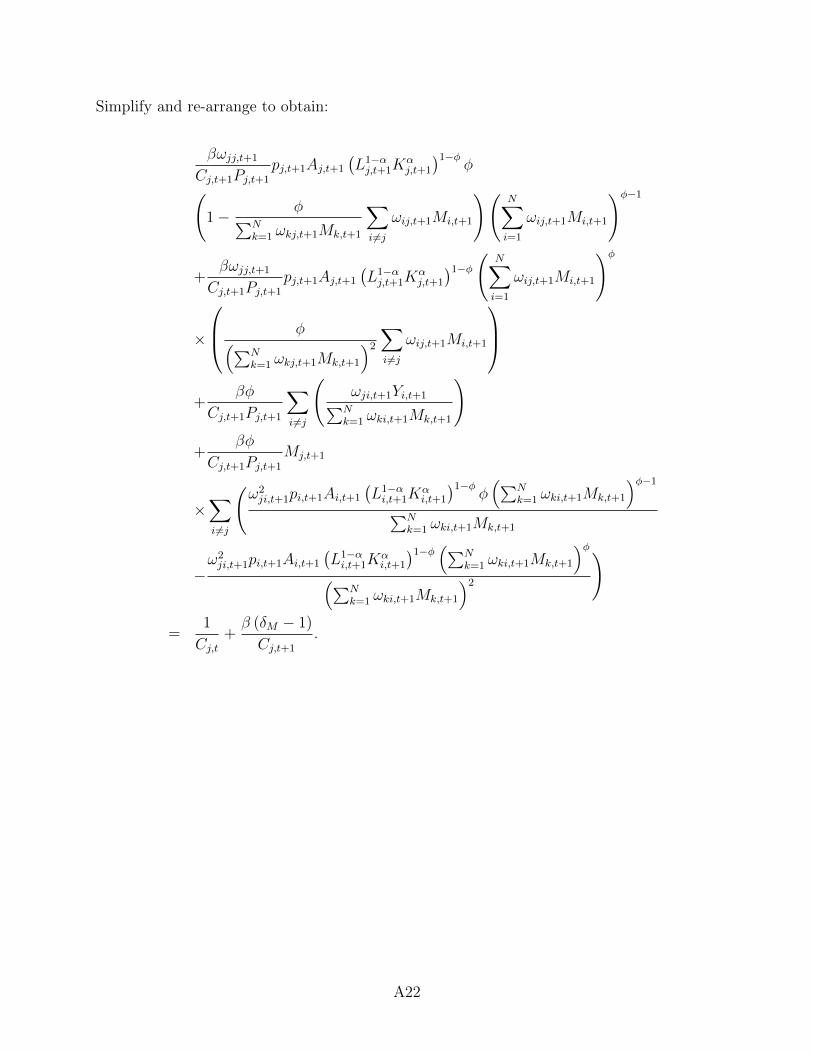
Simplify and re-arrange to obtain:

βωjj,t+1

Cj,t+1Pj,t+1

pj,t+1Aj,t+1

(L1−αj,t+1K

αj,t+1

)1−φφ(

1− φ∑Nk=1 ωkj,t+1Mk,t+1

∑i6=j

ωij,t+1Mi,t+1

)(N∑i=1

ωij,t+1Mi,t+1

)φ−1

+βωjj,t+1

Cj,t+1Pj,t+1

pj,t+1Aj,t+1

(L1−αj,t+1K

αj,t+1

)1−φ(

N∑i=1

ωij,t+1Mi,t+1

)φ

×

φ(∑Nk=1 ωkj,t+1Mk,t+1

)2

∑i6=j

ωij,t+1Mi,t+1

+

βφ

Cj,t+1Pj,t+1

∑i6=j

(ωji,t+1Yi,t+1∑N

k=1 ωki,t+1Mk,t+1

)

+βφ

Cj,t+1Pj,t+1

Mj,t+1

×∑i6=j

(ω2ji,t+1pi,t+1Ai,t+1

(L1−αi,t+1K

αi,t+1

)1−φφ(∑N

k=1 ωki,t+1Mk,t+1

)φ−1

∑Nk=1 ωki,t+1Mk,t+1

−ω2ji,t+1pi,t+1Ai,t+1

(L1−αi,t+1K

αi,t+1

)1−φ(∑N

k=1 ωki,t+1Mk,t+1

)φ(∑N

k=1 ωki,t+1Mk,t+1

)2

)

=1

Cj,t+β (δM − 1)

Cj,t+1

.

A22

Use the definition of Yj,t to re-write the left-hand side of the above expression as:

βωjj,t+1φYj,t+1

Cj,t+1Pj,t+1

(∑Ni=1 ωij,t+1Mi,t+1

)×

(1− φ∑N

k=1 ωkj,t+1Mk,t+1

∑i6=j

ωij,t+1Mi,t+1

)

+βωjj,t+1Yj,t+1

Cj,t+1Pj,t+1

φ(∑Nk=1 ωkj,t+1Mk,t+1

)2

∑i6=j

ωij,t+1Mi,t+1

+

βφ

Cj,t+1Pj,t+1

∑i6=j

(ωji,t+1Yi,t+1∑N

k=1 ωki,t+1Mk,t+1

)

+βφ

Cj,t+1Pj,t+1

Mj,t+1

∑i6=j

(φω2

ji,t+1Yi,t+1(∑Nk=1 ωki,t+1Mk,t+1

)2

−ω2ji,t+1Yi,t+1(∑N

k=1 ωki,t+1Mk,t+1

)2

)

=1

Cj,t

(1

M1−δMj,t

) 1δM 1

δMM

1δM−1

j,t+1 + β1

Cj,t+1

M1δMj,t+2

δM − 1

δMM− 1δM

j,t+1 .

A23

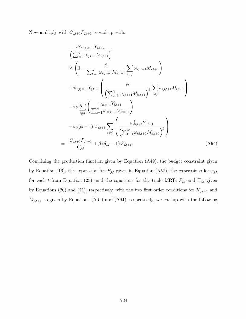
Now multiply with Cj,t+1Pj,t+1 to end up with:

βφωjj,t+1Yj,t+1(∑Ni=1 ωij,t+1Mi,t+1

)×

(1− φ∑N

k=1 ωkj,t+1Mk,t+1

∑i6=j

ωij,t+1Mi,t+1

)

+βωjj,t+1Yj,t+1

φ(∑Nk=1 ωkj,t+1Mk,t+1

)2

∑i6=j

ωij,t+1Mi,t+1

+βφ

∑i6=j

(ωji,t+1Yi,t+1∑N

k=1 ωki,t+1Mk,t+1

)

−βφ(φ− 1)Mj,t+1

∑i6=j

ω2ji,t+1Yi,t+1(∑N

k=1 ωki,t+1Mk,t+1

)2

=

Cj,t+1Pj,t+1

Cj,t+ β (δM − 1)Pj,t+1. (A64)

Combining the production function given by Equation (A49), the budget constraint given

by Equation (16), the expression for Ej,t given in Equation (A52), the expressions for pj,t

for each t from Equation (25), and the equations for the trade MRTs Pj,t and Πj,t given

by Equations (20) and (21), respectively, with the two first order conditions for Kj,t+1 and

Mj,t+1 as given by Equations (A61) and (A64), respectively, we end up with the following

A24

system:

Yj,t = pj,tAj,t(L1−αj,t Kα

j,t

)1−φ(

N∑i=1

ωij,tMi,t

)φ

for all j and t, (A65)

Ej,t = Pj,tCj,t + Pj,t

(Kj,t+1

K1−δKj,t

) 1δK

+ Pj,t

(Mj,t+1

M1−δMj,t

) 1δM

for all j and t, (A66)

Ej,t = Yj,t + φMj,t

∑i6=j

(ωji,tYi,t∑N

k=1 ωki,tMk,t

)(A67)

− φYj,t∑Nk=1 ωkj,tMk,t

∑i6=j

ωij,tMi,t for all j and t, (A68)

pj,t =(Yj,t/Yt)

11−σ

γjΠj,t

for all j and t, (A69)

Yt =N∑j=1

Yj,t for all t, (A70)

P 1−σj,t =

N∑i=1

(tij,tΠi,t

)1−σYi,tYt

for all j and t, (A71)

Π1−σi,t =

N∑j=1

(tij,tPj,t

)1−σEj,tYt

for all i and t, (A72)

α(1− φ)βYj,t+1

Kj,t+1Cj,t+1Pj,t+1

×

(1− φ∑N

k=1 ωkj,t+1Mk,t+1

∑i6=j

ωij,t+1Mi,t+1

)=

1

Cj,t

+β (δK − 1)

Cj,t+1

for all j and t, (A73)

A25

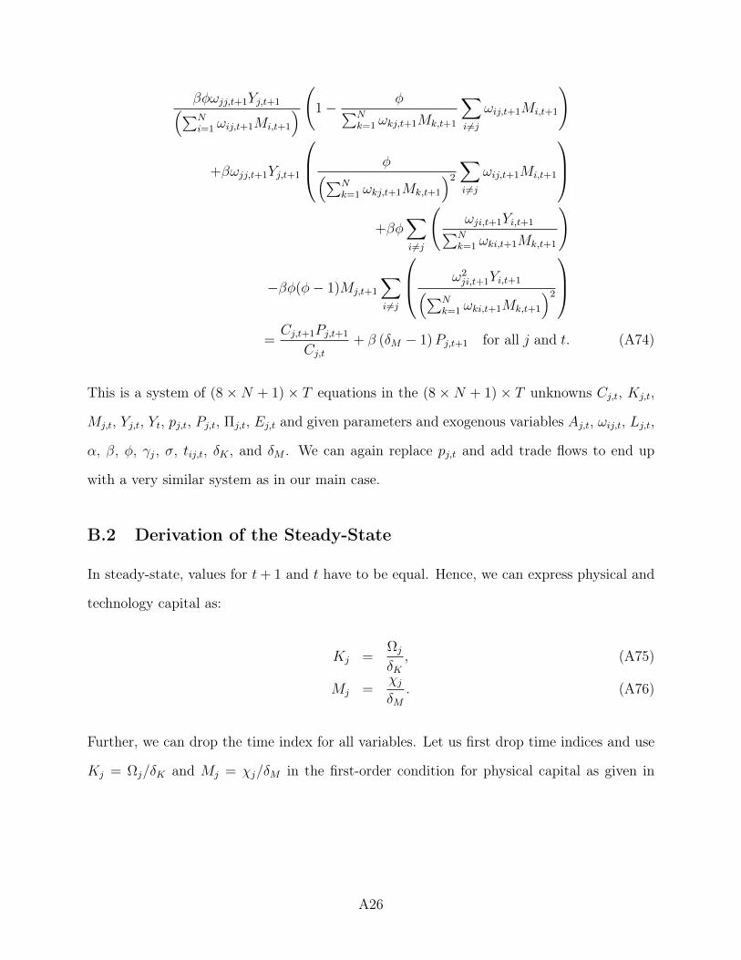
βφωjj,t+1Yj,t+1(∑Ni=1 ωij,t+1Mi,t+1

) (1− φ∑Nk=1 ωkj,t+1Mk,t+1

∑i6=j

ωij,t+1Mi,t+1

)

+βωjj,t+1Yj,t+1

φ(∑Nk=1 ωkj,t+1Mk,t+1

)2

∑i6=j

ωij,t+1Mi,t+1

+βφ

∑i6=j

(ωji,t+1Yi,t+1∑N

k=1 ωki,t+1Mk,t+1

)

−βφ(φ− 1)Mj,t+1

∑i6=j

ω2ji,t+1Yi,t+1(∑N

k=1 ωki,t+1Mk,t+1

)2

=Cj,t+1Pj,t+1

Cj,t+ β (δM − 1)Pj,t+1 for all j and t. (A74)

This is a system of (8 ×N + 1) × T equations in the (8 ×N + 1) × T unknowns Cj,t, Kj,t,

Mj,t, Yj,t, Yt, pj,t, Pj,t, Πj,t, Ej,t and given parameters and exogenous variables Aj,t, ωij,t, Lj,t,

α, β, φ, γj, σ, tij,t, δK , and δM . We can again replace pj,t and add trade flows to end up

with a very similar system as in our main case.

B.2 Derivation of the Steady-State

In steady-state, values for t+ 1 and t have to be equal. Hence, we can express physical and

technology capital as:

Kj =Ωj

δK, (A75)

Mj =χjδM

. (A76)

Further, we can drop the time index for all variables. Let us first drop time indices and use

Kj = Ωj/δK and Mj = χj/δM in the first-order condition for physical capital as given in

A26

Equation (A73):

αβ(1− φ)YjKjCjPj

×

(1− φ∑N

k=1 ωkjMk

∑i6=j

ωijMi

)

=1

Cj+β (δK − 1)

Cjfor all j ⇒

αβ(1− φ)YjKjPj

×

(1− φ∑N

k=1 ωkjMk

∑i6=j

ωijMi

)

= 1 + β (δK − 1) for all j ⇒

αβ(1− φ)YjPj(1− β + βδK)

×

(1− φ∑N

k=1 ωkjMk

∑i6=j

ωijMi

)

= Kj for all j.

Let us next drop time indices and use Kj = Ωj/δK and Mj = χj/δM in the first-order

condition for technology capital as given in Equation (A74):

βφωjjYj(∑Ni=1 ωijMi

) (1− φ∑Nk=1 ωkjMk

∑i6=j

ωijMi

)

+βωjjYj

φ(∑Nk=1 ωkjMk

)2

∑i6=j

ωijMi

+βφ

∑i6=j

(ωjiYi∑N

k=1 ωkiMk

)

−βφ(φ− 1)Mj

∑i6=j

ω2jiYi(∑N

k=1 ωkiMk

)2

=CjPjCj

+ β (δM − 1)Pj for all j ⇒

A27

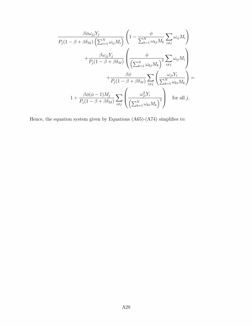
βφωjjYj

Pj(1− β + βδM)(∑N

i=1 ωijMi

) (1− φ∑Nk=1 ωkjMk

∑i6=j

ωijMi

)

+βωjjYj

Pj(1− β + βδM)

φ(∑Nk=1 ωkjMk

)2

∑i6=j

ωijMi

+

βφ

Pj(1− β + βδM)

∑i6=j

(ωjiYi∑N

k=1 ωkiMk

)=

1 +βφ(φ− 1)Mj

Pj(1− β + βδM)

∑i6=j

ω2jiYi(∑N

k=1 ωkiMk

)2

for all j.

Hence, the equation system given by Equations (A65)-(A74) simplifies to:

A28

Yj = pjAj(L1−αj Kα

j

)1−φ(

N∑i=1

ωijMi

)φ

for all j, (A77)

Ej = PjCj + PjKj + PjMj for all j, (A78)

Ej = Yj + φMj

∑i6=j

(ωjiYi∑N

k=1 ωkiMk

)

− φYj∑Nk=1 ωkjMk

∑i6=j

ωijMi for all j, (A79)

pj =(Yj/Y )

11−σ

γjΠj

for all j, (A80)

Y =N∑j=1

Yj, (A81)

P 1−σj =

N∑i=1

(tijΠi

)1−σYiY

for all j, (A82)

Π1−σi =

N∑j=1

(tijPj

)1−σEjY

for all i, (A83)

Kj =αβ(1− φ)Yj

Pj(1− β + βδK)×

(1− φ∑N

k=1 ωkjMk

∑i6=j

ωijMi

)for all j, (A84)

(1 + βδM − β)Pjφβ

=ωjjYj(∑Ni=1 ωijMi

) (1− 1− φ∑Nk=1 ωkjMk

∑i6=j

ωijMi

)

+∑i6=j

(ωjiYi∑N

k=1 ωkiMk

)− (φ− 1)Mj

∑i6=j

ω2jiYi(∑N

k=1 ωkiMk

)2

for all j. (A85)

A29