tractable quanti cation of metastability for robust...
TRANSCRIPT

University of CaliforniaSanta Barbara
Tractable Quantification of Metastability
for Robust Bipedal Locomotion
A dissertation submitted in partial satisfaction
of the requirements for the degree
Doctor of Philosophy
in
Electrical and Computer Engineering
by
Cenk Oguz Saglam
Committee in charge:
Professor Katie Byl, ChairProfessor Andrew R. TeelProfessor Joao P. HespanhaProfessor Bassam BamiehProfessor Art Kuo
June 2015

The Dissertation of Cenk Oguz Saglam is approved.
Professor Andrew R. Teel
Professor Joao P. Hespanha
Professor Bassam Bamieh
Professor Art Kuo
Professor Katie Byl, Committee Chair
June 2015

Tractable Quantification of Metastability
for Robust Bipedal Locomotion
Copyright c© 2015
by
Cenk Oguz Saglam
iii

To my dear family.
Without you, none of this would’ve been possible.
iv

Acknowledgements
I am deeply grateful to my advisor Professor Katie Byl for coming up with such a
fun topic and providing me with ready-to-be-explored research questions, and the most
productive, yet comfortable, laboratory environment for me. Thanks to her support, I got
to enjoy my research with a great independence during all my studies at the University
of California, Santa Barbara.
I am also thankful to all the members of my thesis committee. Professor Andy Teel has
always been easy-to-reach and encouraging all along. I would also like to thank Professor
Joao Hespanha for his invaluable comments both for my research and career. I appreciate
Professor Bassam Bamieh for being available in my committee on such short notice. I am
also honored to have a leading and inspiring researcher of legged locomotion community
like Professor Art Kuo in my committee.
I have always been a proud member of the UCSB Robotics Lab along with Pat
Terry, Chelsea Lau, Sebastian Sovero, Giulia Piovan, Tom Strizic, Brian Satzinger, Hosein
Mahjoubi, and Greg Ray.
I feel very fortunate to meet with so many great people in Santa Barbara. My jour-
ney here started with Alp Yucebilgin as my roommate and continued within a comforting
group formed by Deniz Akdolu, Nazli Dereli, Emre Gul. Back in the days when our algo-
rithms were relatively slow, Emre’s suggestion to use a computer cluster in computation
greatly sped up my progress. As a member of the “Turkish Village”, I gained a whole new
perspective with Bugra Kaytanli, Cetin Sahin, Faruk Gencel, Semih Yavuz, Onur Sinan
Koksaldi, and Omer Ali Acerol. Moreover, thanks to Selim Dogru, a former member of
our village, I will be transitioning to the next step in my career at Intel. In particular,
I really appreciate Bugra’s support as I have been preparing for the next chapter in
my life. Whenever I needed, he devotedly edited numerous texts, including my state-
v

ments, emails, presentations - practically everything, including this sentence (You are
most welcome Oguz).
Of course I would like to thank my beloved family: Abdullah, Cansin, and Aybike
Saglam. Literally (and I mean this) without them I would almost certainly not have
existed. Also without the support of all the members of my family, including my cousins
Burak and Oguz Demirci, this work would not have been possible. I would also like to
thank Beril Pisgin for supporting me from the other side of the earth all these years.
Finally, I would like to thank Institute for Collaborative Biotechnologies for funding
my PhD studies through grant W911NF-09-0001 from the U.S. Army Research Office.
The content of the information does not necessarily reflect the position or the policy of
the Government, and no official endorsement should be inferred.
vi
Curriculum VitæCenk Oguz Saglam
Education
2013-2015 University of California, Santa BarbaraPh.D. in Electrical and Computer EngineeringGPA 4.0/4.0
2011-2013 University of California, Santa BarbaraM.S. in Electrical and Computer EngineeringGPA 4.0/4.0
Summer 2009 University of California, Los AngelesSummer Session in Mechanical and Aerospace Engineering& MathematicsGPA 4.0/4.0
2007-2011 Sabanci University, IstanbulB.S. in Mechatronics EngineeringMinor in MathematicsGPA 3.88/4.0Major GPA: 3.96/4.00
Publications
Cenk Oguz Saglam and Katie Byl. Meshing Hybrid Zero Dynamics for Rough Ter-rain Walking. In Proc. of IEEE International Conference on Robotics and Automation(ICRA), May 2015.
Cenk Oguz Saglam and Katie Byl. Metastable Markov Chains. In IEEE Conferenceon Decision and Control (CDC), December 2014.
Cenk Oguz Saglam, Andrew Teel and Katie Byl. Lyapunov-based versus Poincare MapAnalysis of the Rimless Wheel. In IEEE Conference on Decision and Control (CDC),December 2014.
Cenk Oguz Saglam and Katie Byl. Quantifying the trade-offs between stability versusenergy use for underactuated biped walking. In IEEE/RSJ International Conference onIntelligent Robots and Systems (IROS), 2014.
Cenk Oguz Saglam and Katie Byl. Robust policies via meshing for metastable roughterrain walking. In Proc. of Robotics: Science and Systems (RSS), July 2014.
Cenk Oguz Saglam and Katie Byl. Switching policies for metastable walking. In Proc.of IEEE Conference on Decision and Control (CDC), pages 977-983, December 2013.
vii

Cenk Oguz Saglam and Katie Byl. Stability and gait transition of the five-link bipedon stochastically rough terrain using a discrete set of sliding mode controllers. In Proc. ofIEEE International Conference on Robotics and Automation (ICRA), pages 5675-5682,May 2013.
Cenk Oguz Saglam, Eray A. Baran, Ahmet O. Nergiz and Asif Sabanovic. ModelFollowing Control with Discrete Time SMC for Time-Delayed Bilateral Control Systems.In Proc. of IEEE International Conference on Mechatronics (ICM), pages 997-1002, April2011.
viii

Abstract
Tractable Quantification of Metastability
for Robust Bipedal Locomotion
by
Cenk Oguz Saglam
This work develops tools to quantify and optimize performance metrics for bipedal
walking, toward enabling improved practical and autonomous operation of two-legged
robots in real-world environments. While speed and energy efficiency of legged locomo-
tion are both useful and straightforward to quantify, measuring robustness is arguably
more challenging and at least as critical for obtaining practical autonomy in variable or
otherwise uncertain environmental conditions, including rough terrain. The intuitive and
meaningful robustness quantification adopted in this thesis begins by stochastic model-
ing of disturbances such as terrain variations, and conservatively defining what a failure
is, for example falling down, slippage, scuffing, stance foot rotation, or a combination of
such events. After discretizing the disturbance and state sets by meshing, step-to-step
dynamics are studied to treat the system as a Markov chain. Then, failure rates can be
easily quantified by calculating the expected number of steps before failure. Once robust-
ness is measured, other performance metrics can also be easily incorporated into the cost
function for optimization.
For high performance and autonomous operation under variations, we adopt a ca-
pacious framework, exploiting a hierarchical control structure. The low-level controllers,
which use only proprioceptive (internal state) information, are optimized by a derivative-
free method without any constraints. For practicability of this process, developing an
algorithm for fast and accurate computation of our robustness metric was a crucial and
ix

necessary step. While the outcome of optimization depends on capabilities of the con-
troller scheme employed, the convenient and time-invariant parameterization presented
in this thesis ensures accommodating large terrain variations. In addition, given environ-
ment estimation and state information, the high-level control is a behavioral policy to
choose the right low-level controller at each step. In this thesis, optimal switching policies
are determined by applying dynamic programming tools on Markov decision processes
obtained through discretization. For desirable performance in practice from policies that
are formed using meshing-based approximation to the true dynamics, robustness of high-
level control to environment estimation and discretization errors are ensured by modeling
stochastic noise in the terrain information and belief state while solving for behavioral
policies.
x
This thesis includes the following publications:
• c©2013 IEEE. Reprinted, with permission, from Cenk Oguz Saglam and Katie Byl.
Meshing Hybrid Zero Dynamics for Rough Terrain Walking. In Proc. of IEEE
International Conference on Robotics and Automation (ICRA), May 2015.
• c©2013 IEEE. Reprinted, with permission, from Cenk Oguz Saglam and Katie Byl.
Metastable Markov Chains. In IEEE Conference on Decision and Control (CDC),
December 2014.
• c©2013 IEEE. Reprinted, with permission, from Cenk Oguz Saglam, Andrew Teel
and Katie Byl. Lyapunov-based versus Poincare Map Analysis of the Rimless
Wheel. In IEEE Conference on Decision and Control (CDC), December 2014.
• c©2013 IEEE. Reprinted, with permission, from Cenk Oguz Saglam and Katie Byl.
Quantifying the trade-offs between stability versus energy use for underactuated
biped walking. In IEEE/RSJ International Conference on Intelligent Robots and
Systems (IROS), 2014.
• Reprinted, with permission, from Cenk Oguz Saglam and Katie Byl. Robust policies
via meshing for metastable rough terrain walking. In Proc. of Robotics: Science and
Systems (RSS), July 2014.
• c©2013 IEEE. Reprinted, with permission, from Cenk Oguz Saglam and Katie Byl.
Switching policies for metastable walking. In Proc. of IEEE Conference on Decision
and Control (CDC), pages 977-983, December 2013.
• c©2013 IEEE. Reprinted, with permission, from Cenk Oguz Saglam and Katie Byl.
Stability and gait transition of the five-link biped on stochastically rough terrain
xi
using a discrete set of sliding mode controllers. In Proc. of IEEE International
Conference on Robotics and Automation (ICRA), pages 5675-5682, May 2013.
xii

Contents
1 Introduction 11.1 Stability Measurement for Bipedal Robots . . . . . . . . . . . . . . . . . 21.2 Autonomous Walking . . . . . . . . . . . . . . . . . . . . . . . . . . . . . 101.3 Organization of Thesis . . . . . . . . . . . . . . . . . . . . . . . . . . . . 10
2 Metastable Walking 122.1 Hybrid Model . . . . . . . . . . . . . . . . . . . . . . . . . . . . . . . . . 152.2 Discretization for State Machine Representation . . . . . . . . . . . . . . 152.3 Stochasticity for Markov Decision Process . . . . . . . . . . . . . . . . . 192.4 Eigenanalysis for Stability Metric Development . . . . . . . . . . . . . . 212.5 Toy Example: Rimless Wheel . . . . . . . . . . . . . . . . . . . . . . . . 22
3 Discretization of High-Dimensional States 253.1 Avoiding the Curse of Dimensionality . . . . . . . . . . . . . . . . . . . . 253.2 Explored Meshing . . . . . . . . . . . . . . . . . . . . . . . . . . . . . . . 27
4 Low-Level Control Action 314.1 Optimization of a Given Controller . . . . . . . . . . . . . . . . . . . . . 324.2 Benchmarking Controller Schemes . . . . . . . . . . . . . . . . . . . . . . 354.3 Comparison to Other Work . . . . . . . . . . . . . . . . . . . . . . . . . 374.4 Incorporating Secondary Metrics . . . . . . . . . . . . . . . . . . . . . . 40
5 High-Level Behavioral Policy 425.1 Optimal Policies . . . . . . . . . . . . . . . . . . . . . . . . . . . . . . . . 445.2 Robustness of Switching . . . . . . . . . . . . . . . . . . . . . . . . . . . 525.3 Incorporating Secondary Metrics . . . . . . . . . . . . . . . . . . . . . . 59
6 Conclusions and Future Work 61
A First Passage Value 63A.1 Toy Example: Europe Tour . . . . . . . . . . . . . . . . . . . . . . . . . 64A.2 Absorbing Markov Chains . . . . . . . . . . . . . . . . . . . . . . . . . . 66
xiii

A.3 Mean First Passage Value . . . . . . . . . . . . . . . . . . . . . . . . . . 76A.4 Confidence Levels on Value . . . . . . . . . . . . . . . . . . . . . . . . . . 79A.5 Controlling the Europe Tour . . . . . . . . . . . . . . . . . . . . . . . . . 81A.6 Applications . . . . . . . . . . . . . . . . . . . . . . . . . . . . . . . . . . 82A.7 Conclusion . . . . . . . . . . . . . . . . . . . . . . . . . . . . . . . . . . . 86
B Biped Model 87
C Modeling Rough Terrain 91
D Extended Hybrid Zero Dynamics 93D.1 The Structure . . . . . . . . . . . . . . . . . . . . . . . . . . . . . . . . . 94D.2 Sliding Mode Control . . . . . . . . . . . . . . . . . . . . . . . . . . . . . 95D.3 Swing Phase Zero Dynamics . . . . . . . . . . . . . . . . . . . . . . . . . 96D.4 Hybrid Zero Dynamics Impact . . . . . . . . . . . . . . . . . . . . . . . . 98D.5 Poincare Analysis . . . . . . . . . . . . . . . . . . . . . . . . . . . . . . . 98D.6 Under deterministic conditions . . . . . . . . . . . . . . . . . . . . . . . . 99D.7 Reference Design . . . . . . . . . . . . . . . . . . . . . . . . . . . . . . . 100
Bibliography 103
xiv

List of Figures
1.1 Robots with flat feet . . . . . . . . . . . . . . . . . . . . . . . . . . . . . 41.2 Static stability . . . . . . . . . . . . . . . . . . . . . . . . . . . . . . . . 51.3 Zero moment point . . . . . . . . . . . . . . . . . . . . . . . . . . . . . . 51.4 Dynamic walkers . . . . . . . . . . . . . . . . . . . . . . . . . . . . . . . 8
2.1 Cartoon explaining metastability. . . . . . . . . . . . . . . . . . . . . . . 132.2 Failures in human walking . . . . . . . . . . . . . . . . . . . . . . . . . . 142.3 State machine representation of hybrid dynamics . . . . . . . . . . . . . 182.4 State machine with deterministic control action . . . . . . . . . . . . . . 192.5 Markov chain representation of hybrid stochastic systems . . . . . . . . . 202.6 Metastable dynamics . . . . . . . . . . . . . . . . . . . . . . . . . . . . . 212.7 Illustration of rimless wheel . . . . . . . . . . . . . . . . . . . . . . . . . 222.8 Stability of rimless wheel . . . . . . . . . . . . . . . . . . . . . . . . . . . 24
3.1 Biped with massless legs . . . . . . . . . . . . . . . . . . . . . . . . . . . 263.2 Explored meshing method . . . . . . . . . . . . . . . . . . . . . . . . . . 30
4.1 Optimization of low-level control action . . . . . . . . . . . . . . . . . . . 334.2 Verification of performance quantification . . . . . . . . . . . . . . . . . . 344.3 Benchmarking various controller schemes . . . . . . . . . . . . . . . . . . 364.4 First comparison with the state-of-the-art . . . . . . . . . . . . . . . . . 374.5 Second comparison with the state-of-the-art . . . . . . . . . . . . . . . . 39
5.1 Hierarchical control structure . . . . . . . . . . . . . . . . . . . . . . . . 435.2 Multiple low-level controllers . . . . . . . . . . . . . . . . . . . . . . . . . 455.3 Visual walking . . . . . . . . . . . . . . . . . . . . . . . . . . . . . . . . . 475.4 Blind walking . . . . . . . . . . . . . . . . . . . . . . . . . . . . . . . . . 495.5 Sighted walking . . . . . . . . . . . . . . . . . . . . . . . . . . . . . . . . 515.6 Noisy terrain estimation . . . . . . . . . . . . . . . . . . . . . . . . . . . 535.7 A policy which is robust to sensor noise . . . . . . . . . . . . . . . . . . . 545.8 Performance evaluation on the dense mesh . . . . . . . . . . . . . . . . . 565.9 Stability of the final high-level policy . . . . . . . . . . . . . . . . . . . . 585.10 Incorporation of secondary metrics . . . . . . . . . . . . . . . . . . . . . 60
xv

A.1 Europe tour toy example . . . . . . . . . . . . . . . . . . . . . . . . . . . 65A.2 Traffic intersection toy example . . . . . . . . . . . . . . . . . . . . . . . 85
B.1 Illustration of five-link robot . . . . . . . . . . . . . . . . . . . . . . . . . 88B.2 Hybrid dynamics of walking . . . . . . . . . . . . . . . . . . . . . . . . . 90
C.1 One dimensional terrain disturbances . . . . . . . . . . . . . . . . . . . . 91C.2 Higher dimensional terrain disturbances . . . . . . . . . . . . . . . . . . 92
D.1 Phase instead of time . . . . . . . . . . . . . . . . . . . . . . . . . . . . . 94D.2 Basis functions and their derivatives . . . . . . . . . . . . . . . . . . . . . 101
xvi
List of Tables
4.1 First comparison with the state-of-the-art . . . . . . . . . . . . . . . . . 384.2 Second comparison with the state-of-the-art . . . . . . . . . . . . . . . . 404.3 Incorporation of secondary metrics . . . . . . . . . . . . . . . . . . . . . 40
5.1 Monte Carlo simulations for final high-level control policy . . . . . . . . . 57
A.1 Europe travel information . . . . . . . . . . . . . . . . . . . . . . . . . . 78A.2 States in epidemics . . . . . . . . . . . . . . . . . . . . . . . . . . . . . . 83
B.1 Model parameters for the five-link robot . . . . . . . . . . . . . . . . . . 88
xvii

Chapter 1
Introduction
Over the past few decades, a variety of control methods have made robots quite reliable
in deterministic factory settings. One of the central challenges in robotics today is to
attain robust performance under the variations1 implied by real-world conditions. To
achieve robustness for reliable operation in less-structured environments, quantification
and optimization of relevant performance metrics are essential tasks. Ideally, a robot
should also utilize information about the environment and modify its motion accordingly
to maximize stability and autonomy.
Although the methods presented in this thesis are potentially applicable to autonomous
wheeled vehicles, robotic manipulators, and a broader class of hybrid dynamical systems
in general, the focus is on legged locomotion. In particular, we study two-legged under-
actuated robots walking on rough terrain, for which measuring and achieving stability is
still a major challenge.
While mobility is an undeniable necessity for various robotic applications, one motiva-
tion for bipedal robot walking is that this anthropomorphic approach provides powerful
1 As explained by [Smith, 2012], variations can be categorized as variability, which means “naturalvariation in some quantity”, and uncertainty, which refers to “the degree of precision with which aquantity is measured” [Belle, 2008].
1
Introduction Chapter 1
means for negotiating intermittent or otherwise rough terrain, where wheels would be in-
effective. Bipeds have the capability of moving on steep slopes, climbing ladders, varying
their step width, passing narrow passages, easily turning corners, walking on a tightrope,
avoiding obstacles, and traversing with small footprints. Developments in bipedal locomo-
tion research will enable replacing humans in hazardous jobs, assisting people in difficult
or time consuming tasks, providing better prostheses for the disabled, and rehabilitating
the injured.
1.1 Stability Measurement for Bipedal Robots
Designing and comparing various robotic hardware and/or control schemes require
evaluation of performance using appropriate metrics. In particular, measuring success of
legged locomotion is essential toward developing more capable bipedal robots. Although
the performance of highly-dynamic walkers is often quantified by speed or energy con-
sumption [Hobbelen and Wisse, 2007], these qualities are tangentially meaningful if the
robot is likely to fall in several steps. For reliable operation, the stability of walking must
be measured and increased. Once a robot can walk in an unlikely-to-fall manner, other
metrics such as speed and energy efficiency can be easily incorporated. As an example ap-
plication, control can be optimized to maximize the probability of traversing a particular
terrain with a desired speed and given limited energy capability.
There are two mainstream approaches to bipedal robot design. One approach relies
heavily on ankle torque for balance. By using an appropriately large foot as a base of
support, such robots can be model as fully actuated under carefully controlled operating
conditions. The other approach deliberately uses an underactuated ankle. Without ankle
torque, balance control requires more careful planning, but it also enables more dynamic
gaits, with smaller footholds, better energy efficiency, and potentially greater capabilities
2

Introduction Chapter 1
in regimes where large perturbations to a robot would cause either approach to become
underactuated at the ground contact. The differences in these two approaches’ design
principles lead to qualitatively distinct walking motions and numerous metrics have been
proposed to quantify their stability [Pratt et al., 2001], [Santos et al., 2007], [Hobbelen
and Wisse, 2007], [Byl, 2008], some of which are summarized next.
1.1.1 Flat Footed Humanoids
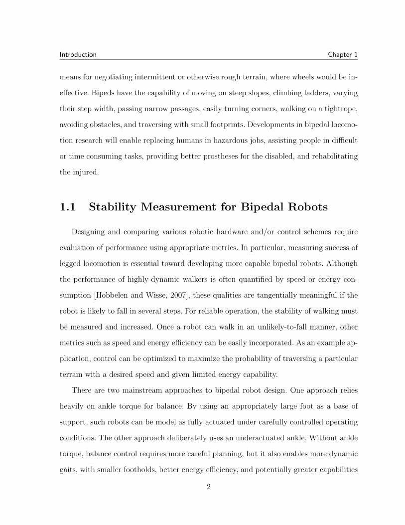
Many well known and very capable humanoids, including the robots shown in Fig-
ure 1.1, are designed to have large feet to make locomotion task relatively easier. Although
humans roll their feet while walking for energy efficiency, these humanoids are often con-
trolled aiming to keep at least one foot flat on the ground at all times. In other words,
the objective is to prevent the foot on the ground from rotating to model robot as fully
actuated. Multiple methods are proposed to achieve such a balance. As [Sugihara, 2009]
explains, these balance criteria are often used to show stability. However, we will later
argue that distinguishing the two is an important step toward human-like walking robots.
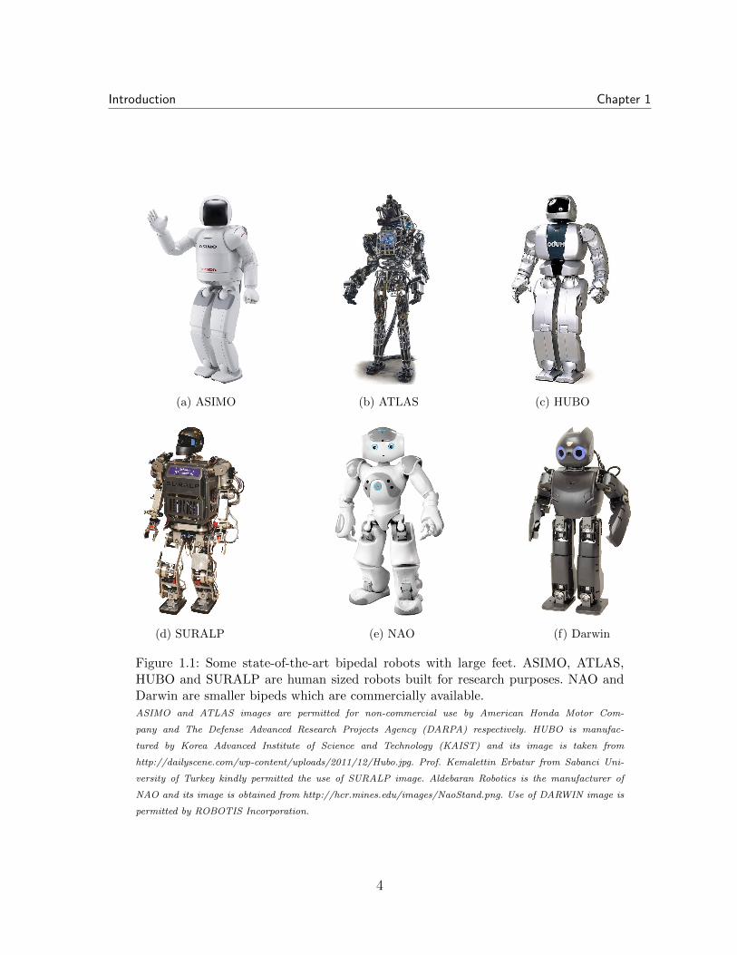
The most elementary approach to balancing is ignoring the kinematics and dynamics
of the system and modeling the robot as a mass with a support polygon2 as shown
in Figure 1.2. In case the projection of this mass’ location to the ground surface is
within the support polygon, the robot is statically stable. Although this approach is
appealing because of its simplicity, given the dynamics of a walker, static stability is
neither necessary nor sufficient condition for keeping the foot flat or walking stably.
Static stability margin concept has been modified in various ways to consider the
kinematics and dynamics of the robot. One extension, which has lead to the most popular
stability metric overall today, focuses on the center of pressure (CoP) on the foot instead
2Convex hull formed by the contacts between the feet and the ground [Tedrake, 2004]. In the 2D case,support polygon is a line, e.g., AB in Figure 1.2.
3
Introduction Chapter 1
(a) ASIMO (b) ATLAS (c) HUBO
(d) SURALP (e) NAO (f) Darwin
Figure 1.1: Some state-of-the-art bipedal robots with large feet. ASIMO, ATLAS,HUBO and SURALP are human sized robots built for research purposes. NAO andDarwin are smaller bipeds which are commercially available.ASIMO and ATLAS images are permitted for non-commercial use by American Honda Motor Com-
pany and The Defense Advanced Research Projects Agency (DARPA) respectively. HUBO is manufac-
tured by Korea Advanced Institute of Science and Technology (KAIST) and its image is taken from
http://dailyscene.com/wp-content/uploads/2011/12/Hubo.jpg. Prof. Kemalettin Erbatur from Sabanci Uni-
versity of Turkey kindly permitted the use of SURALP image. Aldebaran Robotics is the manufacturer of
NAO and its image is obtained from http://hcr.mines.edu/images/NaoStand.png. Use of DARWIN image is
permitted by ROBOTIS Incorporation.
4
Introduction Chapter 1
BPA
CoM
(a) A statically stable object. Static stability mar-
gin is given by min(PA, PB), the minimum dis-
tance from P to the edges of the support polygon.
B PA
CoM
(b) A statically unstable object. Static stability
margin is given by -PB, minus the minimum dis-
tance from P to the edges of the support polygon.
Figure 1.2: Illustration of static stability in 2D. CoM denotes the center of mass.P shows the projection of the CoM. AB, the line segment formed by points A andB, corresponds to the support polygon. If P is in (outside) AB, then the object isstatically stable (unstable).
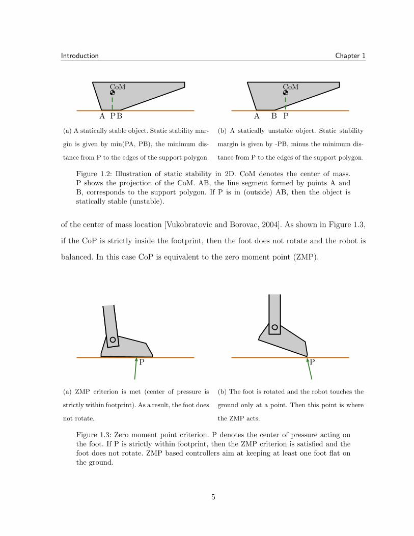
of the center of mass location [Vukobratovic and Borovac, 2004]. As shown in Figure 1.3,
if the CoP is strictly inside the footprint, then the foot does not rotate and the robot is
balanced. In this case CoP is equivalent to the zero moment point (ZMP).
P
(a) ZMP criterion is met (center of pressure is
strictly within footprint). As a result, the foot does
not rotate.
P
(b) The foot is rotated and the robot touches the
ground only at a point. Then this point is where
the ZMP acts.
Figure 1.3: Zero moment point criterion. P denotes the center of pressure acting onthe foot. If P is strictly within footprint, then the ZMP criterion is satisfied and thefoot does not rotate. ZMP based controllers aim at keeping at least one foot flat onthe ground.
5

Introduction Chapter 1
[Goswami and Kallem, 2004] generalizes ZMP concept by proposing a criterion based
on angular momentum to preserve the balance. Algorithms based on linear and angular
momentum have shown to be useful in whole body motion planning and control [Ugurlu
and Kawamura, 2012] [Orin et al., 2013] [Kajita et al., 2003].
Although humanoids are typically controlled to preserve balance to establish stability,
one idea in this thesis is that stability is different than balance. In human-like walking,
each step is basically an intentional “fall” onto the next foot. Avoiding underactuation
for bipeds often results in energy inefficiency. Indeed, the cost of transport3 (CoT) is
estimated to be 0.2 for humans and 3.2 for the infamous humanoid ASIMO shown in
Figure 1.1a [Collins et al., 2005]. On the other hand, [Kuo, 2007] explains that serious
advances in control are necessary to achieve the high versatility of robots like ASIMO
while being as energy efficient as the walkers of next section.
1.1.2 Dynamic Walkers
Toward developing more energy efficient, dynamic, fast, agile and humanlike walk-
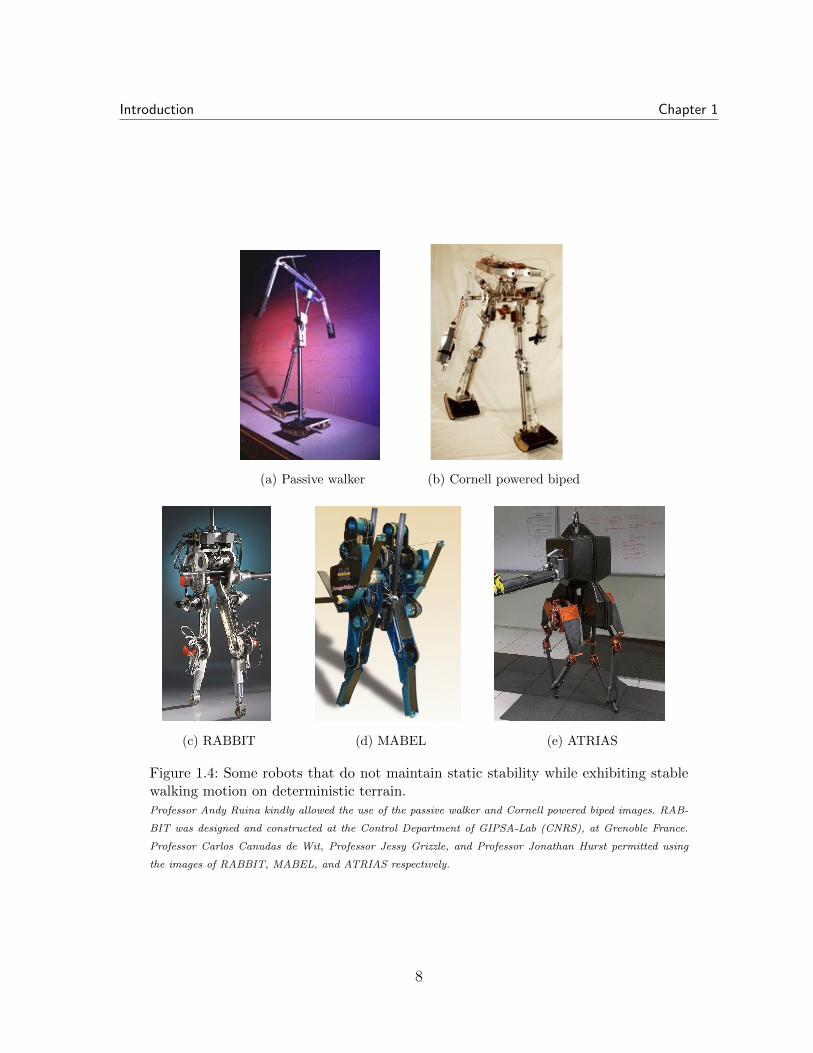
ing robots, Tad McGeer has been inspirational by showing that even passive bipeds
(two-legged walkers that have no motors) can walk downhill in a stable manner using
gravitational forces [McGeer, 1990]. A passive robot built by [Collins et al., 2001] is de-
picted in Figure 1.4a. A key and revolutionary aspect of these machines is that part of
their walking cycle is unbalanced, but the overall walking motion is stable. This prop-
erty, which is ambiguously termed as dynamic walking, has pioneered a major trend in
bipedal locomotion research, where one of the main goals is exploiting underactuation4
like humans rather than avoiding it as in flat footed walking.
3The non-dimensionalized energy expenditure per unit weight and unit distance [Tucker, 1975].4lack of ability to control all degrees-of-freedom. Approximately, the robot in Figure 1.3a is fully
actuated, but it is underactuated in Figure 1.3b.
6

Introduction Chapter 1
Inspired by passive walkers, researchers have demonstrated a range of powered walk-
ers based on exploiting natural dynamics, and the approach has led to record-breaking
performance in walking with only onboard power (energetically autonomous) [Bhounsule
et al., 2014]. Figure 1.4b illustrates the Cornell powered biped designed by [Collins and
Ruina, 2005], which is as energy efficient as humans [Collins et al., 2005].
Although these walkers have been groundbreaking, robots that are designed dom-
inantly for energy efficiency are typically sensitive to perturbations, thus they do not
perform as well as flat footed robots like ASIMO on rough terrain. To close the gap,
various dynamic walkers have been designed for better rough terrain capabilities, three
of which are depicted in the bottom row of Figure 1.4. RABBIT has been a prominent
test bed for theory both in simulation and experiments [Chevallereau et al., 2003]. This
robot was later followed by MABEL, which proved to be a much more capable hardware
on rough terrain [Grizzle et al., 2009]. Using booms, these two robots were constrained
to walk in 2 dimensional space to tackle the problem of understanding underactuated
walking. A more recent point-footed walker is ATRIAS [Hurst, 2015a], which very re-
cently showed the ability to walk in 3D [Hurst, 2015b]. Notice that all three robots are
underactuated because they have point feet to emulate the foot rolling in human loco-
motion. Once the relatively more complicated task of robust walking with no real feet is
achieved, the addition of complex feet and ankle torque only helps toward making the
robot more stable and capable.
Under deterministic conditions, dynamic bipeds exhibit locally stable limit cycles
that repeat once per step. The stability under disturbances is then often studied by local
approximations on these limit cycles by investigating deviations from the trajectories
(gait sensitivity norm [Hobbelen and Wisse, 2007], H∞ cost [Morimioto et al., 2003], and
L2 gain [Dai and Tedrake, 2013]), or the speed of convergence back after such deviations
(using Floquet theory [Hurmuzlu and Basdogan, 1994], [McGeer, 1990]).
7
Introduction Chapter 1
(a) Passive walker (b) Cornell powered biped
(c) RABBIT (d) MABEL (e) ATRIAS
Figure 1.4: Some robots that do not maintain static stability while exhibiting stablewalking motion on deterministic terrain.Professor Andy Ruina kindly allowed the use of the passive walker and Cornell powered biped images. RAB-
BIT was designed and constructed at the Control Department of GIPSA-Lab (CNRS), at Grenoble France.
Professor Carlos Canudas de Wit, Professor Jessy Grizzle, and Professor Jonathan Hurst permitted using
the images of RABBIT, MABEL, and ATRIAS respectively.
8

Introduction Chapter 1
Alternative, the largest single disturbance that the robot can handle without falling
can be measured deterministically [Pratt et al., 2001], [Hobbelen and Wisse, 2007],
[McGeer, 1990]. While this simple idea provides a good intuition for stability, we be-
lieve the expected number of steps before failure metric, described in the next section, is
more suitable for controller optimization, and the process in obtaining it also provides
valuable information to be exploited in Section 1.2.
1.1.3 Expected Number of Steps Before Failure
This thesis adopts and extends a very intuitive and meaningful stability metric intro-
duced by [Byl, 2008], which has been applied to dynamic walkers. It is also potentially
applicable to flat footed humanoids among many other hybrid dynamical systems. [Byl,
2008] presented a methodology to calculate the expected number of steps before failure
under stochastic disturbances, e.g., they assumed slopes ahead of the robot generate a
Gaussian distribution. This analysis can be interpreted either as estimation of failure
rates under disturbances or verification of robustness to these perturbations, depending
on the application.
The method, which is explained in detail in Chapter 2, was originally illustrated
on two and four dimensional systems [Byl and Tedrake, 2009]. Later [Chen and Byl,
2012] applied this machinery to a six dimensional walker. One of the contributions of
this thesis is avoiding the curse of dimensionality to show the applicability of this tool
to even higher dimensional systems by illustrating on a robot with a 10D state space.
The results indicate a clear promise in applications to even higher degrees-of-freedom
humanoids with complex feet walking in 3D.
In addition to calculating expected number of steps before failure, we also extend
the framework to calculate other performance measures under stochastic conditions, e.g.,
9

Introduction Chapter 1
expected speed or energy consumption per step under stochastic conditions, which are
different from the values associated with the limit cycle motion in deterministic environ-
ments. We can also compute metrics like expected distance or (continuous) time before
failure.
1.2 Autonomous Walking
To measure performance, the framework mentioned in Section 1.1.3 works by learning
the dynamics that govern the walking system. This process also provides convenient
means for designing high-level behavioral algorithms that utilize state information and
optional estimation of environmental parameters. Adopting such a hierarchical control
structure does not only increase the stability dramatically, but it also brings autonomy
to the robot. Exploiting this capability is one of the main contributions of this thesis.
High-level control proved to be greatly useful experimentally in [Park et al., 2012],
where a simple policy was employed: If the last step experienced a step-down of more
than 3 cm, “shock absorbing controller” was used. Otherwise the “baseline controller” was
activated. On the other hand, our framework provides a systemic way of obtaining more
complex and optimal policies in more general scenarios. These behavioral algorithms can
also optionally use look-ahead information regarding the terrain when available.
Robots can alternatively utilize information about their environment by kinodynamic
motion planning technique proposed in [Donald et al., 1993]. In comparison, our approach
falls broadly into the machine learning class instead. Once the high-level control policy
is obtained off-line, the only on-line calculation is to use this precomputed look-up ta-
ble at each step to pick the appropriate low-level controller, which makes the approach
compatible with dynamic walking.
10

Introduction Chapter 1
1.3 Organization of Thesis
By focusing on a toy example, the next chapter explains the mathematical tools upon
which the rest of this thesis builds on. The potential curse of dimensionality problem in
using this tool is avoided in Chapter 3, where a powerful meshing method is introduced.
Chapter 4 optimizes and benchmarks control action using the stability metric mentioned
in Section 1.1.3. In addition, Chapter 5 adopts a hierarchical control structure to increase
the performance even more dramatically by optionally using the environmental informa-
tion for autonomous operation. Conclusions and potential future work are presented in
Chapter 6.
11

Chapter 2
Metastable Walking
Metastable systems can be natural or human-made. They exist in a precarious state
of stability, appearing to be locally stable for long periods of time until an external
disturbance perturbs the system into a region of state space with a qualitatively different
local behavior. Since these systems are guaranteed to escape such locally well-behaved
regions with probability one given enough time, they cannot be classified as “stable”, but
it is also misleading to categorize them simply as “unstable”. Physicists have explored this
phenomenon in detail and have developed a number of tools for quantifying metastable
behaviors [Talkner et al., 1987], [Hanggi et al., 1990], [Muller et al., 1997], [Kampen,
2011]. Metastable processes have been observed in many other branches of science and
engineering including familiar systems such as crystalline structures [Larsen and Grier,
1997], flip-flops [Veendrick, 1980], and neuroscience [Fingelkurts and Fingelkurts, 2004].
While focusing on rough terrain walking, this thesis aims to deal with any metastable
system for which escape (fail or success) is guaranteed due to the variations in its environ-
ment. To elaborate, consider the energy profile in Figure 2.1. Assume we start in state-M
and the probability of moving to state-T goes to 1 in time due to the disturbances acting
in the system. Let’s name state-T as transition state, from which we either go back to
12

Metastable Walking Chapter 2
state-M or fall to a stable lower energy state, namely state-S. In this setting, state-M is
not stable in the strict sense because disturbances may result in moving to state-S. How-
ever, if the transitions from state-M to state-T are rare, it is also misleading to categorize
state-M simply as unstable. Since it is “long-living, but destined to eventually end” [Byl,
2008], we classify state-M metastable.
MT
S
State
Energy
Metastablestate
Transitionstate
Stablestate
rare
Figure 2.1: Cartoon explaining metastability. Under deterministic conditions, state-Mis a locally-stable equilibria in a potential. However, with sufficient noise in the model,the particle is guaranteed to transition to lower energy state, namely state-S. If theseguaranteed transitions are extremely rare, states-M is metastable.Figure is inspired from “Meta-stability” by Georg Wiora licensed under GFDL. See [Benallegue and Laumond,
2013] for an inspiring interpretation of metastable walking.
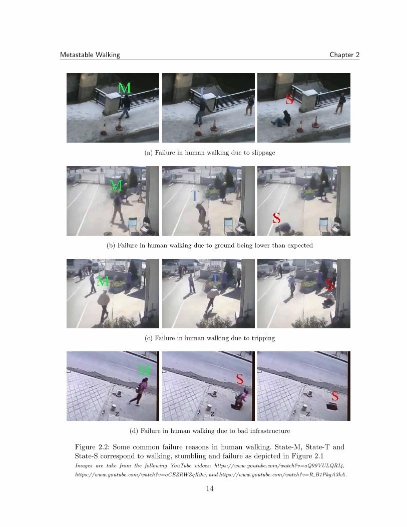
Figure 2.2 shows how states depicted in Figure 2.1 look in human walking. The
key point is to realize that even humans fail in walking from time to time for various
reasons. So, walking is the metastable state in bipedal locomotion, and the transition state
represents staggering or stumbling. In reality, failure to walk is not absorbing because
humans and robots get up after failing. It becomes clear later in the text how, for our
purposes, modeling the failure as a stable state does not ignore the ability to start walking
again.
13
Metastable Walking Chapter 2
(a) Failure in human walking due to slippage
(b) Failure in human walking due to ground being lower than expected
(c) Failure in human walking due to tripping
(d) Failure in human walking due to bad infrastructure
Figure 2.2: Some common failure reasons in human walking. State-M, State-T andState-S correspond to walking, stumbling and failure as depicted in Figure 2.1Images are take from the following YouTube vidoes: https://www.youtube.com/watch?v=aQ99VULQRI4,
https://www.youtube.com/watch?v=oCEZRWZqX9w, and https://www.youtube.com/watch?v=R B1PkgA3kA.
14

Metastable Walking Chapter 2
Before proceeding to mathematical formulation of the framework, we would like to
clarify the notation of state. In the representative image of Figure 2.1, walking is a state.
However, the state of the robot is actually a numeric value denoted by x which changes
while walking. The goal of this chapter is to represent a walking system in the format
shown in Figure 2.1.
2.1 Hybrid Model
Let x, γ, and ζ be the internal state, the randomness system experiences, and the
control action respectively. To illustrate, for a walking robot, x is the robot’s state, γ is
the random variable representing factors such as terrain variation and system noise, and
ζ is the control action which may be a function of x and γ. Define vector y := [x; γ; ζ] to
represent them all. Then, the general hybrid model is represented as
y = f(y) y ∈ C,
y+ = g(y) y ∈ D.(2.1)
C and D are flow and jump sets [Goebel et al., 2012]. This setting is compatible with
less general cases like continuous and discrete systems with/without a control action or
randomness.
2.2 Discretization for State Machine Representation
The first step in discretization precess is choosing a Poincare-like section, noted by
S, such that if the system has not failed yet, it needs to keep passing through this
section. For example, the hybrid dynamics of walking systems are punctuated by discrete
impacts when a foot comes into contact with the ground. These impacts provide a natural
discretization of the robot motion.
15
Metastable Walking Chapter 2
Abuse the notation by letting x refer to the state when y ∈ S. Then, the next state is
a function of the current state x[n], the randomness experienced γ[n], and the controller
action during that step ζ[n], that is
x[n+ 1] = ρ(x[n], γ[n], ζ[n]). (2.2)
To obtain a (discrete) Markov decision process model, finite sets for control action,
randomness, and state are needed. The first one is rather easy, finitely many low-level
controllers are designed which form the controller set Z. The second (randomness),
is straightforward to handle when the number of noise sources is low. For instance,
0, 1k−1
, 2k−1
, ..., 1 is a uniform discretization of [0, 1] with k elements. In this thesis we
study 1 dimensional disturbances and the density of the randomness set Γ is a function
of parameter dγ given by
Γ =
γ :
γ
dγ∈ Z, γl ≤ γ ≤ γr
, (2.3)
where γl and γr determine the range of randomness set, which needs to be wide enough
to model the terrain of interest. Having a wider than needed randomness range has no
disadvantage, but too narrow range causes inaccuracy. In particular, the robot should
not be able to walk at the boundaries of the randomness set, otherwise we extend the
range.
Just like range, density of the randomness set can be chosen depending on the con-
trollers’ performance, and on the robot. Also, the randomness set does not have to be
evenly spaced in general, it may be denser around values of particular interest. As we
increase the density of the randomness set, we are able to capture the dynamics more
accurately at the expense of higher computational costs.
If the internal state x is also low-dimensional, the entire state space can potentially be
uniformly meshed to obtain state set X. However, as dimensionality increases this method
becomes intractable. This potential curse of dimensionality is handled in Chapter 3.
16

Metastable Walking Chapter 2
Once control, randomness and state spaces are represented by finite sets, we simulate
ρ(x, γ, ζ) for each x ∈ X, γ ∈ Γ, and ζ ∈ Z to obtain the state-transition map, which
gives deterministic information about the dynamics. In case the resulting point is not
in the state set, i.e., ρ(x, γ, ζ) 6∈ X, we need to approximate the dynamics. The most
elementary approach is 0’th order approximation given by
x[n+ 1] ≈ c(ρ(x[n], γ[n], ζ[n]), X), (2.4)
where c(x, X) is the closest point x ∈ X to x for the employed distance metric. Then the
deterministic state transition matrix can be written as
T dij(γ, ζ) =
1, if xj = c(ρ(xi, γ, ζ), X)
0, otherwise.
(2.5)
The nearest-neighbor approximation in (2.4) appears to work well in practice. More
sophisticated approximations result in transition matrices not just having one or zero
elements, but also fractional values in between [Abbel, 2012]. This increases memory and
computational costs while, to our experience, not providing much increase in accuracy.
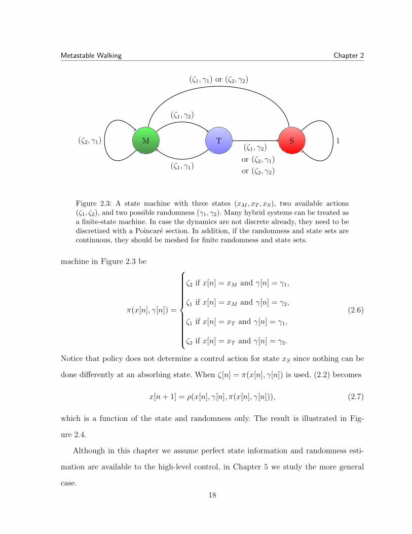
The deterministic state transition matrix corresponds to a state machine similar to
Figure 2.3. In this figure, x[n] ∈ xM , xS, xT, γ[n] ∈ γ1, γ2 and ζ[n] ∈ ζ1, ζ2, which
means there are three states possible, two actions (low-level control) available, and two
random outcomes. Note that given what the randomness is, the transition is deterministic
in this graph.
To derive the Markov chain model we then need to determine a policy π, which is
the high-level control picking the right low-level control action at each step. Chapter 5
is devoted to deriving optimal and robust policies. Let the decided policy for the state
17
Metastable Walking Chapter 2
STM 1
(ζ1, γ1) or (ζ2, γ2)
(ζ1, γ1)
(ζ1, γ2)
(ζ1, γ2)
or (ζ2, γ1)
or (ζ2, γ2)
(ζ2, γ1)
Figure 2.3: A state machine with three states (xM , xT , xS), two available actions(ζ1, ζ2), and two possible randomness (γ1, γ2). Many hybrid systems can be treated asa finite-state machine. In case the dynamics are not discrete already, they need to bediscretized with a Poincare section. In addition, if the randomness and state sets arecontinuous, they should be meshed for finite randomness and state sets.
machine in Figure 2.3 be
π(x[n], γ[n]) =
ζ2 if x[n] = xM and γ[n] = γ1,
ζ1 if x[n] = xM and γ[n] = γ2,
ζ1 if x[n] = xT and γ[n] = γ1,
ζ2 if x[n] = xT and γ[n] = γ2.
(2.6)
Notice that policy does not determine a control action for state xS since nothing can be
done differently at an absorbing state. When ζ[n] = π(x[n], γ[n]) is used, (2.2) becomes
x[n+ 1] = ρ(x[n], γ[n], π(x[n], γ[n])), (2.7)
which is a function of the state and randomness only. The result is illustrated in Fig-
ure 2.4.
Although in this chapter we assume perfect state information and randomness esti-
mation are available to the high-level control, in Chapter 5 we study the more general
case.
18

Metastable Walking Chapter 2
STM 1
γ1
γ2
γ2γ1
Figure 2.4: A state machine with three states (xM , xT , xS) and two possible random-ness (γ1, γ2), which can be obtained from the finite-state machine of Figure 2.3 afterapplying policy π defined in (2.6). Alternatively, this figure is what the model wouldlook like if there was a single low-level controller too. The policy in that case wouldbe using the only available controller.
2.3 Stochasticity for Markov Decision Process
Given deterministic state transition matrix, the last step before obtaining a Markov
chain is to assume a distribution for randomness formulated as
PΓ(γ) := Pr(γ[n] = γ). (2.8)
Then the stochastic state-transition matrix
Tij := Pr(x[n+ 1] = xj | x[n] = xi), (2.9)
which represents the corresponding Markov Chain, can be calculated by
T =∑γ∈Γ
PΓ(γ) T d(γ, ζ). (2.10)
In case ζ[n] = π(x[n], γ[n]), the stochastic matrix becomes
T =∑γ∈Γ
PΓ(γ) T d(γ, π(x, γ)). (2.11)
This last equation will be updated when we consider noise in state information and
randomness estimation in Chapter 5 .
19
Metastable Walking Chapter 2
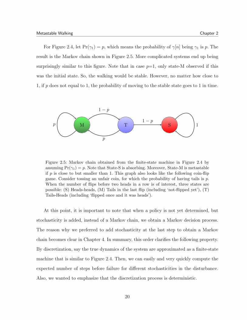
For Figure 2.4, let Pr(γ1) = p, which means the probability of γ[n] being γ1 is p. The
result is the Markov chain shown in Figure 2.5. More complicated systems end up being
surprisingly similar to this figure. Note that in case p=1, only state-M observed if this
was the initial state. So, the walking would be stable. However, no matter how close to
1, if p does not equal to 1, the probability of moving to the stable state goes to 1 in time.
STM 1p
p
1− p
1− p
Figure 2.5: Markov chain obtained from the finite-state machine in Figure 2.4 byassuming Pr(γ1) = p. Note that State-S is absorbing. Moreover, State-M is metastableif p is close to but smaller than 1. This graph also looks like the following coin-flipgame. Consider tossing an unfair coin, for which the probability of having tails is p.When the number of flips before two heads in a row is of interest, three states arepossible: (S) Heads-heads, (M) Tails in the last flip (including ‘not-flipped yet’), (T)Tails-Heads (including ‘flipped once and it was heads’).
At this point, it is important to note that when a policy is not yet determined, but
stochasticity is added, instead of a Markov chain, we obtain a Markov decision process.
The reason why we preferred to add stochasticity at the last step to obtain a Markov
chain becomes clear in Chapter 4. In summary, this order clarifies the following property.
By discretization, say the true dynamics of the system are approximated as a finite-state
machine that is similar to Figure 2.4. Then, we can easily and very quickly compute the
expected number of steps before failure for different stochasticities in the disturbance.
Also, we wanted to emphasize that the discretization process is deterministic.
20

Metastable Walking Chapter 2
2.4 Eigenanalysis for Stability Metric Development
Treating the system as a Markov chain lends itself to a straightforward reliability
measurement. Let λ1 and λ2 be the largest two eigenvalues of the transition matrix
associated with the Markov chain in consideration. Since all failure modes are modeled
to be an absorbing state, λ1 = 1 and the corresponding state distribution, which is called
stationary distribution, has all the probability mass at the failure state.
As explained in detail in Appendix A, after taking several steps without failing, the
robot’s state distribution typically almost converges to metastable distribution. Then, as
shown in Figure 2.6, the robot is able to take the next step successfully with probability
λ2 and it fails otherwise. This allows very easy quantification of stability by
Expected Number of Steps Before Failure =1
1− λ2
. (2.12)
In this calculation we also count the step leading to failure. So, the expected number of
steps before failure is larger than or equal to 1.
SM 1λ2
1-λ2
Figure 2.6: Metastable dynamics. As explained in detail in Appendix A, after takingseveral steps without failing, the robot’s state distribution typically almost convergesto metastable distribution, which is represented by the green ball on the left. The robotis able to take the next step successfully with probability λ2, which implies mappingback to the metastable distribution. Otherwise the robot transitions to failure state,which is represented by the red ball on the right. Then, the stability of walking onrough terrain can be easily quantified by (2.12).
21

Metastable Walking Chapter 2
2.5 Toy Example: Rimless Wheel
As a toy example, in this section we study the system shown in Figure 2.7, where the
slope may change at each step1. After the introduction of passive dynamic walking in
[McGeer, 1990] over two decades ago, the rimless wheel has become very popular in loco-
motion research because this uncomplicated walker keeps many of the essential properties
of dynamic walking robots [Bhounsule, 2014]. For simplicity, we focus on forward walk-
ing only and assume the mass is lumped to the center of the robot and equals m=1 kg,
length of each leg is given by l=1 m, number of legs is 8, gravitational acceleration is
κ=9.81 m/s2, and legs never slip, i.e., the friction is always enough. For a more general
and detailed approach to the rimless wheel compared to this section refer to [Saglam
et al., 2014].
2αl
m−γ
θ
κ
Figure 2.7: The rimless wheel as depicted in [Byl and Tedrake, 2009]. We define for-ward direction to be to the right (i.e., clockwise). The state for this walker is twodimensional, consisting of the angle θ and velocity ω = θ. Negative γ values corre-spond to downhill.
The single support phase is when only one leg is in contact with the ground. This
phase has continuous pendulum dynamics given by θ = κ sin(θ). The leg in contact with
the ground is referred to as the stance leg. On the other hand, double support phase is
1See Appendix C for terrain modeling.
22
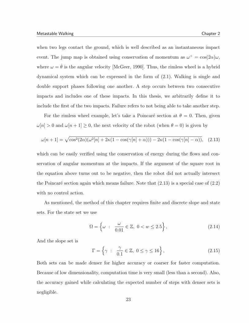
Metastable Walking Chapter 2
when two legs contact the ground, which is well described as an instantaneous impact
event. The jump map is obtained using conservation of momentum as ω+ = cos(2α)ω,
where ω = θ is the angular velocity [McGeer, 1990]. Thus, the rimless wheel is a hybrid
dynamical system which can be expressed in the form of (2.1). Walking is single and
double support phases following one another. A step occurs between two consecutive
impacts and includes one of these impacts. In this thesis, we arbitrarily define it to
include the first of the two impacts. Failure refers to not being able to take another step.
For the rimless wheel example, let’s take a Poincare section at θ = 0. Then, given
ω[n] > 0 and ω[n+ 1] ≥ 0, the next velocity of the robot (when θ = 0) is given by
ω[n+ 1] =√
cos2(2α)(ω2[n] + 2κ(1− cos(γ[n] + α)))− 2κ(1− cos(γ[n]− α)), (2.13)
which can be easily verified using the conservation of energy during the flows and con-
servation of angular momentum at the impacts. If the argument of the square root in
the equation above turns out to be negative, then the robot did not actually intersect
the Poincare section again which means failure. Note that (2.13) is a special case of (2.2)
with no control action.
As mentioned, the method of this chapter requires finite and discrete slope and state
sets. For the state set we use
Ω =ω :
ω
0.01∈ Z, 0 < w ≤ 2.5
, (2.14)
And the slope set is
Γ =γ :
γ
0.1∈ Z, 0 ≤ γ ≤ 16
, (2.15)
Both sets can be made denser for higher accuracy or coarser for faster computation.
Because of low dimensionality, computation time is very small (less than a second). Also,
the accuracy gained while calculating the expected number of steps with denser sets is
negligible.
23
Metastable Walking Chapter 2
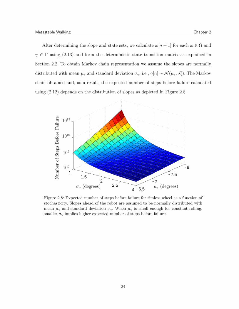
After determining the slope and state sets, we calculate ω[n+ 1] for each ω ∈ Ω and
γ ∈ Γ using (2.13) and form the deterministic state transition matrix as explained in
Section 2.2. To obtain Markov chain representation we assume the slopes are normally
distributed with mean µγ and standard deviation σγ, i.e., γ[n] ∼ N (µγ, σ2γ). The Markov
chain obtained and, as a result, the expected number of steps before failure calculated
using (2.12) depends on the distribution of slopes as depicted in Figure 2.8.
11.5
22.5
3 6.5
7
7.5
80
5
10
151015
1010
105
100 -
-
-
-σγ (degrees) µγ (degrees)
Num
ber
ofSte
ps
Bef
ore
Fai
lure
Figure 2.8: Expected number of steps before failure for rimless wheel as a function ofstochasticity. Slopes ahead of the robot are assumed to be normally distributed withmean µγ and standard deviation σγ . When µγ is small enough for constant rolling,smaller σγ implies higher expected number of steps before failure.
24

Chapter 3
Discretization of High-Dimensional
States
In applying the tool of Chapter 2, one of the steps was meshing the state space to represent
it with finitely many elements, e.g., 0, 1k−1
, 2k−1
, ..., 1 is a uniform discretization of [0, 1]
with k elements. However, uniformly meshing the entire state space becomes intractable
for high dimensional systems. Thus, as mentioned in Section 2.2, there is potentially
a curse of dimensionality for high degrees-of-freedom robots. However, if the intrinsic
dimension of the reachable state space is low, meshing can still be achieved for systems
with high-dimensional states as explained in this chapter.
3.1 Avoiding the Curse of Dimensionality
The critical observation toward avoiding the curse of dimensionality is the fact that
only the reachable state space under the given control law needs to be meshed instead of
the entire state space. Let us illustrate with the simple biped model shown in Figure 3.1.
This walker has two massless legs and one actuator which controls the inter-leg angle.
25

Discretization of High-Dimensional States Chapter 3
Assuming second order dynamics, the state space is 4 dimensional for this walker, con-
sisting of 2 angles and 2 velocities. To begin with, assume that immediately after each
impact, the controller ensures q = 2α and q = 0. In this case, this walker is identical to
the rimless wheel we studied in Section 2.5 where 2α corresponds to the fixed inter-leg
angle. Note that although this simple biped has a 4D state, the reachable state space
under the mentioned control law is only 2 dimensional.
q
l
mγ
θ
κ
Figure 3.1: Illustration of a very simple biped model. The legs are massless and theonly actuator controls the inter-leg angle q. Assuming that immediately after eachimpact the controller ensures q = 2α and q = 0, then this biped behaves like therimless wheel in Figure 2.7.
In reality, the controller may not be able to reach its references before every impact.
To maximize the allowed time for converge, we take the Poincare section just before
impacts instead of θ = 0 as in Section 2.5. However, even after this choice, the controller
may not be able to perfectly convergence in some cases, so the reachable state space
typically turns out to be a quasi -2D manifold. Note that the rimless wheel has 1 degree-
of-freedom (DOF) but no actuators, and the massless legged biped has 2 DOF and 1
actuator. So, both these walkers are underactuated by 1 DOF. Similarly, the 5-link biped
modeled in Appendix B is also underactuated by 1 DOF, because it has 5 links and 4
actuators. As a result, the reachable state space under a given control law turns out to
be a quasi-2D manifold for the 5-link biped also [Saglam and Byl, 2013a].
26
Discretization of High-Dimensional States Chapter 3
We note that the reachable state space being a lower dimensional manifold is not an
intrinsic requirement for our meshing technique, which is presented next. This section
is rather an explanation why the following method does not explode and instead stays
tractable when applied to high DOF robots.
3.2 Explored Meshing
Determining the state set is difficult because we are studying high dimensional sys-
tems, e.g., the 5-link walker has a 10 dimensional state (i.e., positions and velocities).
So, it is not feasible to uniformly and densely cover a hypercube that includes the reach-
able state space. However, meshing the reachable state space can be achieved by starting
from an initial state set Xi with very small number of points (one “good” state, such as
the fixed point under mean disturbance, is enough) and deterministically expanding by
iteratively simulating.
Our algorithm works as follows. We initially start by setting X = x ∈ Xi : x 6= x11,
which corresponds to all non-failure states that are not simulated yet. Then we start the
following iteration: As long as there is a state x ∈ X, simulate to find all possible ρ(x, γ, ζ)
and remove x from X. For the points newly found, check their distance to the other states
in X. If the distance is larger than some threshold dthr, i.e., the point is far enough from
all existing mesh points, then add that point to X and X. We call the mesh obtained by
this method explored-mesh and present the pseudocode in Algorithm 1.
Using the right distance metric is crucial in ensuring that X has a small number
of states while accurately covering the reachable state space. Standardized (normalized)
Euclidean distance turned out to be extremely useful as it dynamically adjusts the weights
for each dimension according to its standard deviation at any mesh iteration. The distance
1As explained in Appendix A, without loss of generality x1 represents all the failures no matter howrobot failed.
27

Discretization of High-Dimensional States Chapter 3
Algorithm 1 Explored meshing algorithm
Input: Initial set of states Xi, Randomness set Γ, Controller set Z, and threshold dis-
tance dthrOutput: Final set of states X, and state-transition map
1: X ← Xi (except x1)
2: X ← Xi
3: while X is non-empty do
4: X2 ← X
5: empty X
6: for each state x ∈ X2 do
7: for each slope γ ∈ Γ do
8: for each controller ζ ∈ Z do
9: Simulate a single step to get the final state x when initial state is x,
slope ahead is γ, and controller ζ is used (Calculate x = ρ(x, γ, ζ)).
Store this information in the state-transition map
10: if robot did not fall (x 6= x1) and d(x,X) > dthr then
11: add x to X
12: add x to X
13: end if
14: end for
15: end for
16: end for
17: end while
28

Discretization of High-Dimensional States Chapter 3
of a vector x from X is calculated as
d(x, X) := minx∈X
∑i
(xi − xiri
)2, (3.1)
where ri is the standard deviation of i’th dimension of all existing points in set X. In
addition, the closest point in X to x is given by
c(x, X) := argminx∈X
∑i
(xi − xiri
)2. (3.2)
Our algorithm allows us to increase the accuracy of the final mesh at the expense of
producing a higher number of states (larger X) by decreasing threshold distance dthr for
states and discretization length dγ used for randomness set in (2.3).
While meshing the whole 10D state space for the 5-link walker we study in this thesis
is infeasible, this method is able to avoid the curse of dimensionality because the reachable
state space is actually a quasi-2D manifold as explained in the first section.
For the rimless wheel, Figure 3.2 shows the explored mesh obtained using dthr = 0.025
and dγ = 0.5. Points in this figure correspond to possible states just before impacts. The
probability of being at each state is shown with color. Convex hulls of states that cover
the 0.9, 0.99, 0.999, and 0.9999 of the state probability distribution are also drawn.
In Section 2.5 the state mesh was only 1 dimensional because we took a Poincare
section at θ = 0. As we focus on the states just before the impact in this chapter, the
reachable state space is rather 2 dimensional. However, we obtain similar results using
both methods. In particular, let’s consider uniformly distributed slope changes with mean
µγ = 7 and standard deviation σγ = 1 for the rimless wheel. Under these circumstances,
we calculated the expected number of steps to be 1.79×10⁷ and 2.1×10⁷ in the previous
chapter and using explored mesh of Figure 3.2 respectively.
29

Discretization of High-Dimensional States Chapter 3
0.4 0.45 0.5 0.55 0.6 0.651.2
1.4
1.6
1.8
2
2.2
2.4
2.6
Angle (radians)
Ang
ular
Vel
ocity
(ra
dian
s/se
c)
0
0.02
0.04
0.06
0.08
Figure 3.2: Explored meshing method applied on the rimless wheel in Figure 2.7.Threshold distance dthr = 0.025 and slope set discretization length dγ = 0.5 wereused to obtain a mesh with 252 states shown in this figure. Colored bar depicts theprobability of being at a state at the end of a step while walking. Convex hulls cover0.9, 0.99, 0.999, and 0.9999 of the state probability distribution. The expected numberof steps is calculated to be 2.1× 10⁷ using this mesh.
3.2.1 Two Tricks
Two important tricks to make the explored meshing algorithm run faster are as fol-
lows. First, the randomness set allows a natural cluster analysis. The distance comparison
for a new point can be made only with the points that are associated with the same slope.
This might result in more points in the final mesh, but it speeds up the meshing and
later calculations significantly. Secondly, fix a controller ζ and a state x. Then we can
simulate ρ(x,min(Γ), ζ) and then potentially extract ρ(x, γ, ζ) for all γ ∈ Γ. To illustrate,
in order for the robot to experience an impact at −30 degree, it has to pass through all
the possible impact points with higher degrees, and we can extract all impact cases from
a single simulation.
30

Chapter 4
Low-Level Control Action
Performance of highly-dynamic walkers is often quantified by speed or energy consump-
tion under deterministic conditions [Hobbelen and Wisse, 2007]. However, legged robots
need “good” disturbance rejection to operate reliably in real-world environments, and
achieving this goal requires quantifying robustness. Out of the small number of metrics
proposed for measuring robustness of dynamic walkers, the L2 gain calculation in [Dai
and Tedrake, 2013] was successfully extended and implemented on a real robot in [Grif-
fin and Grizzle, 2015]. Alternatively, largest terrain disturbance was maximized in [Pratt
et al., 2001] and trajectories were optimized to replicate human-walking data in [Ames,
2012]. Instead, this thesis adopts the metric explained in Chapter 2, which is used to opti-
mize and benchmark control action in this chapter. We argue that this approach provides
better performance on rough terrain and it is more powerful for benchmarking purposes.
Mostly, we study the particular control strategy formulated in Appendix D as a case
demonstration. However, two other control schemes are also optimized for benchmarking
purposes. The first one is the now-familiar hybrid zero dynamics approach [Westervelt
et al., 2003] and the other is a method using piece-wise reference trajectories with a
sliding mode control [Saglam and Byl, 2013b].
31

Low-Level Control Action Chapter 4
For optimization, we employ the “fminsearch” in MATLAB R©, which uses the derivative-
free method proposed by [Lagarias et al., 1998] to find the unconstrained minimum. In
case we impose constraints, we use the extended version provided by [Oldenhuis, 2009]
instead.
4.1 Optimization of a Given Controller
As mentioned, control action is often designed to minimize energy consumption or
maximize speed. For the first one, Cost of Transport (COT) gives the non-dimensionalized
energy expenditure per unit weight and unit distance [Tucker, 1975]. It is defined as the
total mechanical energy spent, divided by weight times distance, i.e.,
COT =W
mgd, (4.1)
where m is the mass, g is the gravitational constant, and d is the distance traveled. In
this paper we use the conservative definition of “energy spent” by regarding negative
work is also done by the robot, i.e.
W = |Wpositive|+ |Wnegative| = Wpositive −Wnegative (4.2)
so that both acceleration and breaking require power, but there is no regenerative break-
ing. Compared to energy efficiency, measuring speed under deterministic conditions is
even more straightforward.
To evaluate the stability obtained by optimizing for these metrics, we consider nor-
mally changing the slopes in front of the robot as in Figure C.1a. We fix the long-term
mean slope to be µγ = 0 and vary the standard deviation σγ to calculate resulting
expected number of steps before failure depicted in Figure 4.1. The results reveal that
optimizing for these metrics results in sensitivity to perturbations, thus performing poorly
on rough terrain as expected.
32
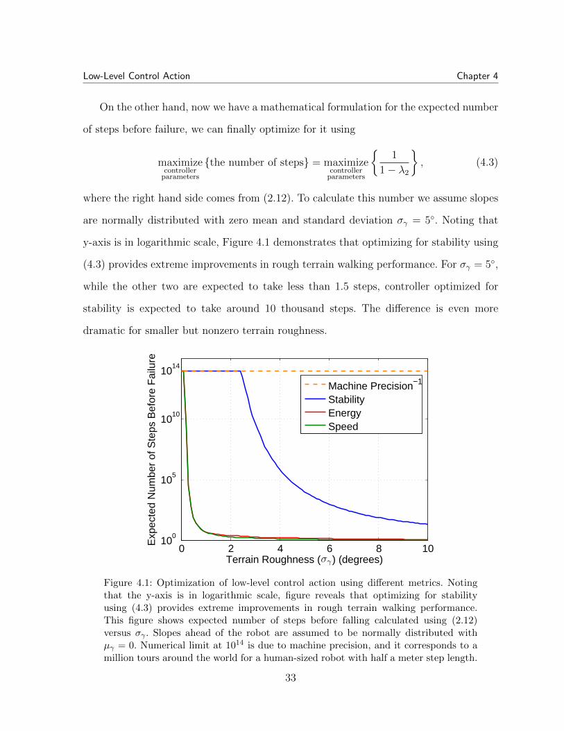
Low-Level Control Action Chapter 4
On the other hand, now we have a mathematical formulation for the expected number
of steps before failure, we can finally optimize for it using
maximizecontroller
parameters
the number of steps = maximizecontroller
parameters
1
1− λ2
, (4.3)
where the right hand side comes from (2.12). To calculate this number we assume slopes
are normally distributed with zero mean and standard deviation σγ = 5. Noting that
y-axis is in logarithmic scale, Figure 4.1 demonstrates that optimizing for stability using
(4.3) provides extreme improvements in rough terrain walking performance. For σγ = 5,
while the other two are expected to take less than 1.5 steps, controller optimized for
stability is expected to take around 10 thousand steps. The difference is even more
dramatic for smaller but nonzero terrain roughness.
0 2 4 6 8 1010
0
105
1010
1014
Terrain Roughness ( ) (degrees)
Exp
ecte
d N
umbe
r of
Ste
ps B
efor
e F
ailu
re
Machine Precision−1
StabilityEnergySpeed
σγ
Figure 4.1: Optimization of low-level control action using different metrics. Notingthat the y-axis is in logarithmic scale, figure reveals that optimizing for stabilityusing (4.3) provides extreme improvements in rough terrain walking performance.This figure shows expected number of steps before falling calculated using (2.12)versus σγ . Slopes ahead of the robot are assumed to be normally distributed withµγ = 0. Numerical limit at 1014 is due to machine precision, and it corresponds to amillion tours around the world for a human-sized robot with half a meter step length.
33

Low-Level Control Action Chapter 4
Note that the number of points in the final mesh, and the accuracy obtained from
(2.12) with this mesh, are inversely related to parameters dthr and dγ, where dthr is the
threshold distance in Algorithm 1 and dγ is the discretization length in (2.3). We claim
that, as dγ → 0 and dthr → 0, the mesh captures the true, hybrid dynamic system
dynamics, and as a result, the expected number of steps before failure for the controllers,
converges. To test the accuracy of our calculations, we evaluate the performance of the top
controller in Figure 4.1 using (dthr, dγ) ∈ (2, 2.5), (1, 1), (0.5, 0.5). The fine mesh, which
is obtained using (dthr, dγ) = (0.5, 0.5), has 77,329 states, and the coarse mesh, which is
a result of using (dthr, dγ) = (2, 2.5), consists of only 372 states. Figure 4.2 demonstrates
the convergence of performance quantification with indistinguishable curves.
0 2 4 6 8 1010
0
105
1010
1014
Terrain Roughness ( ) (degrees)
Exp
ecte
d N
umbe
r of
Ste
ps B
efor
e F
ailu
re
Machine Precision−1
Coarse (372 states)Medium (5,470 states)Fine (77,329 states)Monte Carlo Simulations
σγ
Figure 4.2: Verification of performance quantification. The fine mesh is obtained using(dthr, dγ) = (0.5, 0.5), and the coarse mesh is a result of using (dthr, dγ) = (2, 2.5).Closely matching curves and data points indicate our performance quantification isaccurate. This figure shows expected number of steps before falling calculated using(2.12) versus σγ . Slopes ahead of the robot are assumed to be normally distributedwith µγ = 0. Numerical limit at 1014 is due to machine precision, and it correspondsto a million tours around the world for a human-sized robot with half a meter steplength.
34

Low-Level Control Action Chapter 4
For further verification of our results, we also carry Monte Carlo simulations for σ ∈
7, 8, 9, 10. For each case we simulate 104 times until failure. The average number of
steps are also provided in Figure 4.2. Closely matching results validates our approach once
again. At this point we would like to clarify some clear advantages of our methodology
over Monte Carlo simulations. While obtaining a single point in Figure 4.2 required
“104×average number of steps” simulations for Monte Carlo method, all of the curve
associated with the coarse mesh was obtained by 372 simulations only! So, with far fewer
simulations we were able to create a whole curve instead of getting a single data point.
This is because once the system is discretized, addition of stochasticity and calculation
of λ2 are fast operations. Note that Monte Carlo simulations become quickly intractable
as the number of steps increases, whereas the numerical limit in our method is very high
and can be enlarged by increasing the machine precision when necessary. Furthermore,
calculating the curve is just one of the outcomes in our methodology. This complete tool,
for example, also provides invaluable information for high-level control design as we will
see in the next chapter.
[Benallegue and Laumond, 2013] presents a method based on Monte Carlo simulations
to compute the expected number of steps before failure when it is very high. The method
relies on the property that for a fixed controller dynamic walkers return very close to
their limit-cycle over and over again as they keep walking. In a future work, this method
will be used to verify the curves in Figure 4.2 also for low σγ values.
4.2 Benchmarking Controller Schemes
In addition to optimization capabilities, benchmarking is a powerful use of our math-
ematical tool, which we already employed to present Figure 4.1 and 4.2. In this section,
we look at how different controller schemes optimized for stability compare. The first one
35
Low-Level Control Action Chapter 4
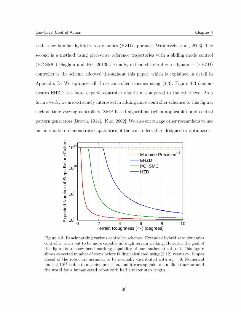
is the now-familiar hybrid zero dynamics (HZD) approach [Westervelt et al., 2003]. The
second is a method using piece-wise reference trajectories with a sliding mode control
(PC-SMC) [Saglam and Byl, 2013b]. Finally, extended hybrid zero dynamics (EHZD)
controller is the scheme adopted throughout this paper, which is explained in detail in
Appendix D. We optimize all three controller schemes using (4.3). Figure 4.3 demon-
strates EHZD is a more capable controller algorithm compared to the other two. As a
future work, we are extremely interested in adding more controller schemes to this figure,
such as time-varying controllers, ZMP-based algorithms (when applicable), and central
pattern generators [Brown, 1914], [Kuo, 2002]. We also encourage other researchers to use
our methods to demonstrate capabilities of the controllers they designed or optimized.
0 2 4 6 8 1010
0
105
1010
1014
Terrain Roughness ( ) (degrees)
Exp
ecte
d N
umbe
r of
Ste
ps B
efor
e F
ailu
re
Machine Precision−1
EHZDPC−SMCHZD
σγ
Figure 4.3: Benchmarking various controller schemes. Extended hybrid zero dynamicscontroller turns out to be more capable in rough terrain walking. However, the goal ofthis figure is to show benchmarking capability of our mathematical tool. This figureshows expected number of steps before falling calculated using (2.12) versus σγ . Slopesahead of the robot are assumed to be normally distributed with µγ = 0. Numericallimit at 1014 is due to machine precision, and it corresponds to a million tours aroundthe world for a human-sized robot with half a meter step length.
36

Low-Level Control Action Chapter 4
4.3 Comparison to Other Work
We finally compare our results with the state-of-the-art. Like this thesis, [Dai and
Tedrake, 2013] adopts the RABBIT robot model provided in Appendix B. However,
instead of using normal distributions as we have done so far, they uniformly distribute
the slopes ahead of the robot. Then, they optimize a time-varying control structure for
the L2 gain to minimize deviations due to ground variations. To test their resulting
controller, they assume the slopes ahead of the robot is normally distributed between
-2 and +2 degrees and simulate 40 times until failure. The robot takes 20.325 steps
on average as depicted in Figure 4.4, where our controller greatly outperforms in terms
of stability. Note that to obtain the curve for our controller, we did not discretize the
0 5 10 15 20 25 3010
0
105
1010
1014
Terrain Roughness ( ) (degrees)
Exp
ecte
d N
umbe
r of
Ste
ps B
efor
e F
ailu
re
Machine Precision−1
Saglam and Byl ’15Dai and Tedrake ’13
a
Figure 4.4: First comparison with the state-of-the-art. Our controller outperformsthe [Dai and Tedrake, 2013] and we were able to present our results with more datapoints using fewer simulations. This figure shows expected number of steps beforefalling calculated using (2.12) versus a. Slopes ahead of the robot are assumed to beuniformly distributed between ±a degrees. Numerical limit at 1014 is due to machineprecision, and it corresponds to a million tours around the world for a human-sizedrobot with half a meter step length.
37

Low-Level Control Action Chapter 4
dynamics again. We simply used our discretization from the previous section and added
a different form of stochasticity. The computation took only several seconds.
We would like to explain why there is a sudden fall in expected number of steps around
σγ = 14 in Figure 4.4 unlike the previous 2 figures, where we used normal distributions.
Say the slopes are normally distributed between ±a degrees. Imagine a robot which can
walk in a stable manner when a = 14 degrees. Assume the robot falls in two steps beyond
this limit. Now, if we look at a = 12.5, then we should expect to hit the numerical limit
in Figure 4.4. However, if a = 15, then there is around 1/152 ≈ 0.00444 chance the robot
will fail after the following two steps, which corresponds to only 225 steps on average.
On the other hand, when we employ normal distributions we consider a very wide range
of slopes possible with finite probabilities for all, which might be extremely small at the
tails. But this gives us smooth transitions and allows calculating any σγ value, whereas
calculations for a values outside slope set are not always trustable. That’s why Figure 4.4
only uses the data points shown to form the curve, while the previous two figures uses a
much denser standard deviation set, so each data point are not shown to avoid clutter.
In addition to Figure 4.4, we also followed the method in [Dai and Tedrake, 2013]
and simulated 40 times until failure independent from the discretization process. Instead
of limiting slopes between -2 and +2 degrees, where our robot seems unlikely to fall, we
used -17.5 and +17.5 degrees to take 77.525 steps on average as listed in Table 4.1.
Table 4.1: First comparison with the state-of-the-art. Slopes ahead of the robot arechanging uniformly. Simulations are carried 40 times until failure.
Terrain AverageRoughness Number of Steps
Hongkai Dai and Russ Tedrake, 2013 [−2, 2] 20.325
Cenk Oguz Saglam and Katie Byl, 2015 [−17.5, 17.5] 77.525
38

Low-Level Control Action Chapter 4
In another state-of-the-art work, [Griffin and Grizzle, 2015] again uses uniform dis-
tribution, but this time instead of slopes ahead of the robot, step heights change as
illustrated in Figure C.1b. They simulate 50 times until failure, but they limit each it-
eration to 104 steps to reduce computational cost. They report that their controller was
able finish 4 of the 50 trials when step heights are uniformly distributed between ±4 cm.
On average the robot takes 4,616 as shown in Figure 4.5. In comparison, although our
0 2 4 6 8 1010
0
105
1010
1014
Terrain Roughness ( ) (cm)
Exp
ecte
d N
umbe
r of
Ste
ps B
efor
e F
ailu
re
Machine Precision−1
Saglam and Byl ’15Griffin and Grizzle ’15
a
Figure 4.5: Second comparison with the state-of-the-art. Our controller also outper-forms the [Griffin and Grizzle, 2015] and we were able to present our results with moredata points using fewer simulations. This figure shows expected number of steps beforefalling calculated using (2.12) versus a. Step heights ahead of the robot are assumedto be uniformly distributed between ±a. Numerical limit at 1014 is due to machineprecision, and it corresponds to a million tours around the world for a human-sizedrobot with half a meter step length.
controller was optimized for a normally distributed sloped terrain, it outperforms on a
uniformly distributed step terrain as shown in Figure 4.5. Independently from this figure,
we also simulated 50 times when step heights are uniformly distributed between ±4 cm,
and our robot was able to complete all trials as listed in Table 4.2. We should also note
that while we and [Dai and Tedrake, 2013] are working on RABBIT shown in Figure 1.4c,
39

Low-Level Control Action Chapter 4
[Griffin and Grizzle, 2015] use a model for ATRIAS pictured in Figure 1.4e.
Table 4.2: Second comparison with the state-of-the-art. Step heights ahead of the robotare changing uniformly. Simulations are carried 50 times until failure or reaching thelimit at 104 steps.
Terrain FinishedRoughness Trials
Brent Griffin and Jessy Grizzle, 2015 [−4, 4] cm 4/50
Cenk Oguz Saglam and Katie Byl, 2015 [−4, 4] cm 50/50
4.4 Incorporating Secondary Metrics
Finally, once stability is quantified, it is straightforward to incorporate other met-
rics. To illustrate, the controller parameters obtained using (4.3) turns out to produce a
relatively slow walking motion as shown in Table 4.3. However, if we allow extra room
for the optimization to also consider other metrics, we obtain walking gaits that are
faster and more energy efficient as the table demonstrates. The cost function given by
2×COT−speed was empirically chosen and the potential trade-off can be easily adjusted
depending on the application.
The fact that optimal controller depends on what the objective (or cost) function is
motivates adopting the hierarchical control structure of the next chapter. In particular,
section 5.3 studies the advantages of switching between the two controllers listed in
Table 4.3.
40

Low-Level Control Action Chapter 4
Table 4.3: Incorporating secondary metrics on low-level control design. The secondcolumn gives the expected number of steps before failure when slopes are normallydistributed with zero mean and standard deviation equals 5 degrees.
Expected Number of Steps Speed COT
maximizecontroller
parameters
1
1− λ2
≈ 104 0.462 0.212
minimizecontroller
parameters
2× COT− speed≈ 102 0.7 0.185
subject to1
1− λ2
≥ 102
41

Chapter 5
High-Level Behavioral Policy
What is very intuitive but has lacked sufficient attention in the robotics community
is that humans do not walk the same way on every ground type. They modify their
walk depending on various conditions, such as whether the surface is pavement or clay,
whether the ground is triangular (slopes), or rectangular (stairs), whether it’s uphill
or downhill, and whether there are obstacles on the way, just to name some terrain
features. It is not possible or necessary to design a specific controller for each specific
case. However, if we have multiple controllers (potentially designed with different general
cases in mind) available, the robot may increase stability by appropriately switching
among controllers. While switching using only internal (proprioceptive) state information
(blind-walking) is advantageous [Park et al., 2012], [Saglam and Byl, 2014c], a dramatic
improvement is obtained with use of upcoming terrain information [Saglam and Byl,
2013b]. Instead, work to date has typically focused either on remaining robust when blind
to upcoming terrain [Raibert et al., 2008], [Park et al., 2013] or on achieving particular
footstep lengths [Hodgins and Raibert, 1991], without more generally addressing the issue
of planning on partly-known terrain. In this chapter we propose a systematic way to solve
this problem.
42

High-Level Behavioral Policy Chapter 5
Figure 5.1 displays the hierarchical control structure adopted in this thesis, which
features a high-level control picking one of the low-level controllers at each step. As
expressed in Chapter 2 when there are multiple low-level controllers available to the
robot, discretization yields a Markov decision process, which is solved to obtain a Markov
chain and to quantify reliability. In the general form, policies (high-level controllers)
are functions of the state estimation and noisy terrain information. Simpler policies are
special cases in this setting. The goal is to obtain robust, near-optimal control policies
for low-level controllers using dynamic programming tools [Bellman, 1957], [Saglam and
Byl, 2014c].
High-LevelController
State
Slope
Torque
ζ−10 ζ−5 ζ5ζ0 ζ10Low-LevelControllers
Figure 5.1: Hierarchical control structure. At each step, the high-level controller picksa low-level controller to use given state estimation and optional noisy terrain informa-tion. In this figure there are five low-level controllers available. ζi denotes the low-levelcontrol optimized for a normally distributed terrain with mean µγ = i degrees andstandard deviation σγ = 5 using Chapter 4’s method.
43

High-Level Behavioral Policy Chapter 5
Let ζi denote the low-level control optimized for a normally distributed terrain with
mean µγ = i degrees and standard deviation σγ = 5 using Chapter 4’s method. To begin
with, we use the controller set given by Z = ζ−10, ζ−5, ζ0, ζ5, ζ10 and discretize the
dynamics using Algorithm 1 with dthr = 1 and dγ = 1. The resulting mesh has 59,804
states.
5.1 Optimal Policies
In this section we look at the benefits of using environment and state information to
switch between low-level controllers. Initially we assume none of these are available to
the robot, so the policy is to use one of the fixed controllers. Then we investigate the
improvements gained by using slope or state information only. In these cases the robot
is said to do visual or blind walking respectively. On the other hand, in general a policy
is a function of both slope and state estimation, so the policy is given by
ζ[n] = π(x[n], γ[n]), (5.1)
as used in Chapter 2. We refer to this choice as sighted walking.
5.1.1 Fixed Controllers
The simplest policy is to use just one controller, i.e.,
ζ[n] = ζi (5.2)
for fixed i. In this case T is calculated as in (2.10) for a given µγ and σγ. We then derive
the expected number of steps before failure using (2.12). To evaluate the performance of
the individual controllers in Z depending on the long-term mean slope, we fix σγ to be
5 degrees. The results are demonstrated in Figure 5.2, where the x-axis is µγ, and the
y-axis shows the expected number of steps before failure.
44

High-Level Behavioral Policy Chapter 5
We note that the optimal choice for using one of the fixed controllers in Z depends
on the long term mean slope. If the mean slope is close to 0 degrees, the fixed controller
policy needs to be using ζ0 for optimality.
−30 −20 −10 0 10 20 3010
0
101
102
103
104
105
Mean Slope of the Terrain Ahead ( ) (degrees)
Exp
ecte
d N
umbe
r of
Ste
ps B
efor
e F
ailu
re
ζ−10
ζ−5
ζ0
ζ5
ζ10
µγ
Figure 5.2: Performance of individual low-level controllers. Let ζi denote the low-levelcontrol optimized for a normally distributed terrain with mean µγ = i degrees andstandard deviation σγ = 5 using Chapter 4’s method. The controllers shown in thispicture are ζ−10, ζ−5, ζ0, ζ5, and ζ10 from left to right. The expected numbers of stepsbefore falling are calculated using (2.12) versus µγ . Slopes ahead of the robot areassumed to be normally distributed with σγ = 5 deg.
45

High-Level Behavioral Policy Chapter 5
5.1.2 Visual Walking
After seeing that the performance of the individual controllers depends significantly
on the mean slope ahead, we consider policies using only one-step lookahead (γ[n]) in-
formation, which are in the form of
ζ[n] = π(γ[n]). (5.3)
A trivial idea is to look at the slope ahead and using the controller which was opti-
mized for the nearest slope. In other words, π(γ[n]) = ζi and i = c(γ, −10,−5, 0, 5, 10),
where function c is as defined in (3.2). To illustrate, we use controller ζ0 when −2.5 ≤
γ ≤ 2.5. We present the performance of this trivial policy in Figure 5.3. It is rather sur-
prising to see how bad this intuitive policy turns out to be. To improve the performance,
we used genetic algorithm to obtain the visual policy given by
π(γ[n]) =
ζ−10, γ ≤ −28.5
ζ−5, −28.5 < γ ≤ −17.5
ζ0, −17.5 < γ ≤ 24.5
ζ5, 24.5 < γ ≤ 29.5
ζ10, 29.5 < γ,
(5.4)
which performs better when µγ = 0.
Although the improvements gained by using slope estimation seem to be small in
this specific case, we later discover in the following sections that single-step lookahead to
terrain is very useful when used together with state information.
46

High-Level Behavioral Policy Chapter 5
−30 −20 −10 0 10 20 3010
0
101
102
103
104
105
Mean Slope of the Terrain Ahead ( ) (degrees)
Exp
ecte
d N
umbe
r of
Ste
ps B
efor
e F
ailu
re
Visual
Trivial
ζ−10
ζ−5
ζ0
ζ5
ζ10
µγ
Figure 5.3: Performance of a two visual policies. The trivial high-level controller usesπ(γ[n]) = ζi and i = c(γ, −10,−5, 0, 5, 10), where function c is as defined in (3.2).To illustrate, it picks ζ0 when −2.5 ≤ γ ≤ 2.5. Visual policy is defined in (5.4).See Figure 5.2 to distinguish five fixed controllers shown in this picture. The expectednumbers of steps before falling are calculated using (2.12) versus µγ . Slopes ahead ofthe robot are assumed to be normally distributed with σγ = 5 deg.
47
High-Level Behavioral Policy Chapter 5
5.1.3 Blind (to the terrain) Walking
In practice the robot knows its state and it is typical to assume policy to be a function
of the state in Markov Decision Processes, i.e.,
ζ[n] = π(x[n]). (5.5)
The optimal policy is commonly solved using value iteration [Bellman, 1957], which works
by recursively calculating
V (i) := maxζ
∑j
Pij(ζ) (R(j) + α V (j))
, (5.6)
where V is the value, Pij(ζ) is the probability of transitioning from xi to xj when ζ is
used, R(j) is the reward for transitioning to xj, and α ∈ [0, 1] is the discount factor,
which is chosen to be 0.9. This equation is iterated until convergence to get the optimal
policy.
Remember that the failure state is x1. The value of the failure state is initially set to
zero, i.e.,
V (1) = 0, (5.7)
and it always stays as zero, because the reward for taking a successful step is one, while
falling is zero, i.e.,
R(j) =
0, j = 1,
1, otherwise.
(5.8)
Note that the reward function we use does not depend on the controller, slope ahead,
or current state. Use of more sophisticated reward functions (e.g., considering energy,
speed, step width) is a topic of Section 5.3 and [Saglam and Byl, 2014b]. However, our
initial focus is only on stability in this chapter. Substituting (5.7) and (5.8) into (5.6)
yields
V (i) := maxζ
∑j 6=1
Pij(ζ) (1 + α V (j))
. (5.9)
48

High-Level Behavioral Policy Chapter 5
The probability of ‘transitioning from xi to xj when ζ is used’ is
Pij(ζ) =∑γ∈Γ
PΓ(γ) T dij(γ, ζ). (5.10)
So we can alternatively write the value iteration algorithm as
V (i) := maxζ
∑γ∈Γ
PΓ(γ)∑j 6=1
T dij(γ, ζ) (1 + α V (j))
. (5.11)
Optimization results for µγ = 0 and σγ = 5 deg are shown in Figure 5.4. In the light of
this figure, we conclude that even blindly switching between the controllers may provide
dramatic improvements on the overall performance. However, it is also important to note
that we have not studied discretization errors yet. So, Figure 5.4 may be overselling the
improvements obtained by blind-to-the-terrain switching.
−30 −20 −10 0 10 20 3010
0
101
102
103
104
105
Mean Slope of the Terrain Ahead ( ) (degrees)
Exp
ecte
d N
umbe
r of
Ste
ps B
efor
e F
ailu
re
Blind ζ−10
ζ−5
ζ0
ζ5
ζ10
µγ
Figure 5.4: Blind walking. The high-level controller knows the state but it is blindto the environment. Value iteration is used to get the optimal policy. See Figure 5.2to distinguish five fixed controllers shown in this picture. The expected numbers ofsteps before falling are calculated using (2.12) versus µγ . Slopes ahead of the robotare assumed to be normally distributed with σγ = 5 deg.
49
High-Level Behavioral Policy Chapter 5
5.1.4 Sighted Walking
In sighted walking the high-level controller uses both the state information and one-
step lookahead to terrain, i.e., the policy is given by (5.1). To use the one-step lookahead
in deriving policy, we modify the value iteration in (5.11) as
V (i) :=∑γ∈Γ
maxζ
PΓ(γ)
∑j 6=1
T dij(γ, ζ) (1 + α V (j))
. (5.12)
So, maximization operation is carried for each slope in Γ.
Instead of modifying the value iteration algorithm, we could define a new 11D state,
including the slope in addition to the 10D state of the robot. However, (5.12) makes
the analysis of the following parts easier, reduces computational cost, and requires less
memory. Note that PΓ(γ) gives the probability of ‘the slope ahead being γ’ and T dij(γ, ζ)
is the probability of ‘transitioning from xi to xj when ζ is used and the slope is γ’.
We optimize for µγ = 0 and σγ = 5 degrees to get the performance shown in Figure 5.5.
Noting the logarithmic y-axis, it is clear that sighted walking is significantly better than
visual and blind walking, as one would intuitively expect. The ability to quantify this
intuition is a driving goal of our work.
Although the optimal high-level control in Figure 5.5 is obtained by optimizing for
µγ = 0 and σγ = 5 degrees, the figure demonstrates that it also performs well for µγ 6= 0.
In the following sections we observe that the same argument follows for σγ 6= 5 degrees.
The dramatic improvement gained by using one-step terrain lookahead along with
state information motivates measuring how much a two-, three- and infinite-step looka-
head increases the stability, which is a topic of future work.
50

High-Level Behavioral Policy Chapter 5
−30 −20 −10 0 10 20 3010
0
101
102
103
104
105
106
Mean Slope of the Terrain Ahead ( ) (degrees)
Exp
ecte
d N
umbe
r of
Ste
ps B
efor
e F
ailu
re
Optimal ζ−10
ζ−5
ζ0
ζ5
ζ10
µγ
Figure 5.5: Sighted walking. The high-level controller uses both the state informationand one-step lookahead to terrain. See Figure 5.2 to distinguish five fixed controllersshown in this picture. The expected numbers of steps before falling are calculated using(2.12) versus µγ . Slopes ahead of the robot are assumed to be normally distributedwith σγ = 5 deg.
51

High-Level Behavioral Policy Chapter 5
5.2 Robustness of Switching
Although Figure 5.5 is impressive, for this methodology to be applicable to real-life
problems, policies must be robust to uncertainties. In particular, considering the noise
in the inputs of high-level controller is crucial. So, in this section we study and improve
robustness of sighted walking to terrain estimation and state information. The results
motivate experimenting the methods and controllers of this thesis on a real robot.
5.2.1 Noisy Terrain Estimation
We start our robustness study by considering the addition of noise to slope informa-
tion. The slope ahead is still defined by variable γ, but let’s say the controller thinks it
is (closest to) γ ∈ Γ, due to the noise l ∈ Γ. The relationship is given by
γ = max(min(Γ),min(max(Γ), γ + l)). (5.13)
Note that this equation simply says γ = γ+ l except at boundaries of the slope set. PL(l)
is defined by
PL(l) := Pr(l[n] = l), (5.14)
and normally distributed with zero mean and standard deviation σl, i.e.,
l[n] ∼ N (0, σ2l ). (5.15)
In the presence of noise, the policy is a function of γ, not γ. Thus, we have
ζ[n] = π(x[n], γ[n]). (5.16)
Then the stochastic state-transition matrix in (2.10) becomes
T =∑γ∈Γ
∑l∈Γ
PΓ(γ) PL(l) T d(γ, π(x, γ)). (5.17)
52
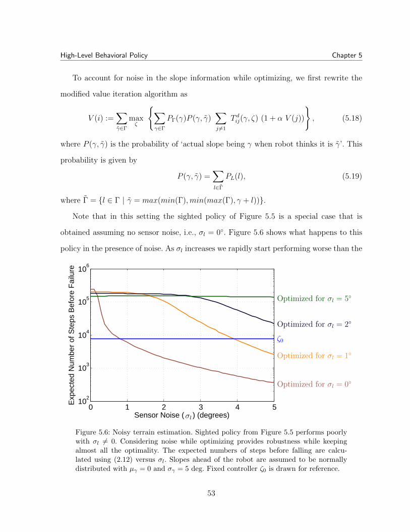
High-Level Behavioral Policy Chapter 5
To account for noise in the slope information while optimizing, we first rewrite the
modified value iteration algorithm as
V (i) :=∑γ∈Γ
maxζ
∑γ∈Γ
PΓ(γ)P (γ, γ)∑j 6=1
T dij(γ, ζ) (1 + α V (j))
, (5.18)
where P (γ, γ) is the probability of ‘actual slope being γ when robot thinks it is γ’. This
probability is given by
P (γ, γ) =∑l∈Γ
PL(l), (5.19)
where Γ = l ∈ Γ | γ = max(min(Γ),min(max(Γ), γ + l)).
Note that in this setting the sighted policy of Figure 5.5 is a special case that is
obtained assuming no sensor noise, i.e., σl = 0. Figure 5.6 shows what happens to this
policy in the presence of noise. As σl increases we rapidly start performing worse than the
0 1 2 3 4 510
2
103
104
105
106
Sensor Noise ( ) (degrees)
Exp
ecte
d N
umbe
r of
Ste
ps B
efor
e F
ailu
re
ζ0
Optimized for σl = 0
Optimized for σl = 1
Optimized for σl = 2
Optimized for σl = 5
σl
Figure 5.6: Noisy terrain estimation. Sighted policy from Figure 5.5 performs poorlywith σl 6= 0. Considering noise while optimizing provides robustness while keepingalmost all the optimality. The expected numbers of steps before falling are calcu-lated using (2.12) versus σl. Slopes ahead of the robot are assumed to be normallydistributed with µγ = 0 and σγ = 5 deg. Fixed controller ζ0 is drawn for reference.
53
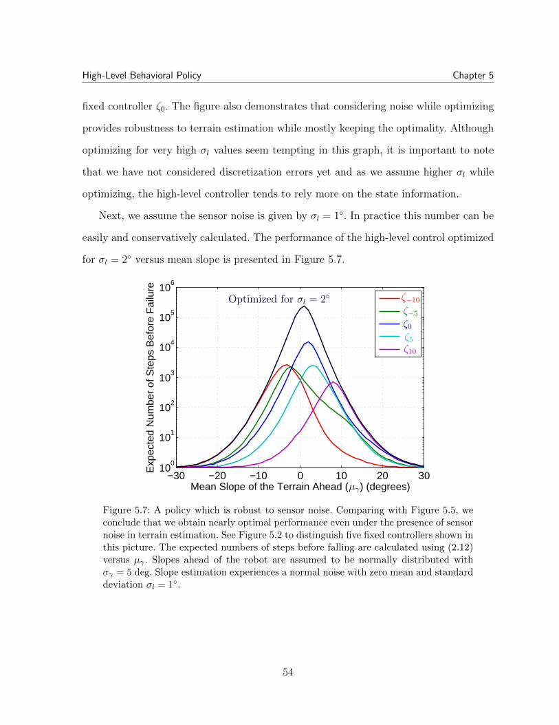
High-Level Behavioral Policy Chapter 5
fixed controller ζ0. The figure also demonstrates that considering noise while optimizing
provides robustness to terrain estimation while mostly keeping the optimality. Although
optimizing for very high σl values seem tempting in this graph, it is important to note
that we have not considered discretization errors yet and as we assume higher σl while
optimizing, the high-level controller tends to rely more on the state information.
Next, we assume the sensor noise is given by σl = 1. In practice this number can be
easily and conservatively calculated. The performance of the high-level control optimized
for σl = 2 versus mean slope is presented in Figure 5.7.
−30 −20 −10 0 10 20 3010
0
101
102
103
104
105
106
Mean Slope of the Terrain Ahead ( ) (degrees)
Exp
ecte
d N
umbe
r of
Ste
ps B
efor
e F
ailu
re
Optimized for σl = 2 ζ−10
ζ−5
ζ0
ζ5
ζ10
µγ
Figure 5.7: A policy which is robust to sensor noise. Comparing with Figure 5.5, weconclude that we obtain nearly optimal performance even under the presence of sensornoise in terrain estimation. See Figure 5.2 to distinguish five fixed controllers shown inthis picture. The expected numbers of steps before falling are calculated using (2.12)versus µγ . Slopes ahead of the robot are assumed to be normally distributed withσγ = 5 deg. Slope estimation experiences a normal noise with zero mean and standarddeviation σl = 1.
54

High-Level Behavioral Policy Chapter 5
5.2.2 Discretization Errors
Up until now, we optimized policies and evaluated resulting performance using the
same (dthr = 1) mesh. In this section, we keep optimizing on the coarse (dthr = 1) mesh,
but we estimate performance using a denser, more refined (dthr = 0.7) mesh, intended
to better approximate the true system dynamics. The high-resolution mesh, which has
199,358 states, is used to tune the real performance of high-level control and ensure its
robustness to discretization errors. First, we need to explain how the coarse-mesh policy
can be applied when the noisy slope ahead estimation γ[n] may not be in the slope set,
and/or state x[n] may not be in the mesh. In these cases, we apply the most basic idea
formulated by
ζ[n] = π(c(x[n], X), c(γ[n],Γ)), (5.20)
where function c is as defined in (3.2). In its general form, let us denote the dense mesh
by Xd, which is obtained from a slope set Γd. Using this mesh, we can approximate how
(5.20) would behave in practice by
ζ[n] = π(c(xd[n], X), c(γd[n],Γ)), (5.21)
where xd ∈ Xd and γd ∈ Γd. The definition and calculation of T remain the same,
but this time Xd and Γd is used in obtaining it. Figure 5.8 shows that the policy from
Figure 5.7 performs poorly when evaluated on the dense mesh. We must once again refine
our algorithm, this time to improve robustness to meshing discretization.
In our approach to fix this issue, we consider the following: While the actual state
is xi, the robot may think it is xk. To make this clear, we rewrite the value iteration
algorithm as
V (k) :=∑γ∈Γ
maxζ
∑γ∈Γ
PΓ(γ)P (γ, γ)∑i
P (i, k)∑j 6=1
T dij(γ, ζ) (1 + α V (j))
, (5.22)
where P (i, k) is the probability of ‘actual state being xi when robot thinks it is xk’.
55

High-Level Behavioral Policy Chapter 5
0 2 4 6 8 1010
0
103
106
109
1012
Terrain Roughness ( ) (degrees)
Exp
ecte
d N
umbe
r of
Ste
ps B
efor
e F
ailu
re
Machine Precision−1
Low−Level ControlHigh−Level ControlMonte Carlo Simulations
Policy from Figure 5.7
(ζ0)
σγ
Figure 5.8: Performance evaluation on the dense mesh. The policy from Figure 5.7performs poorly. However, discretization errors can be handled to obtain the robustpolicy shown in this graph. Compare to Figure 4.2, where the stability of low-levelcontroller was verified with Monte Carlo simulations. The expected numbers of stepsbefore falling are calculated using (2.12) versus σγ . Slopes ahead of the robot are as-sumed to be normally distributed with µγ = 0. Sensor noise is given by σl = 1. Fixedcontroller ζ0 is drawn for reference. Numerical limit at 1012 is due to machine preci-sion, and it corresponds to a 10 thousand tours around the world for a human-sizedrobot with half a meter step length.
Finding the best calculation for P (i, k) is an open question. However, it is intuitive
that for a given state k (the robot thinks the state is xk), P (i, k) should be smaller for
i for which d(xi, xk) is larger. Among many other methods, inverse distance weighting
as in [Shepard, 1968] did not provide desirable performance. In [Saglam and Byl, 2014c],
we illustrate that an exponential distribution works well. In this thesis, to show the
applicability of various distributions, we use power distribution given by
P (i, k) =λc∑c λ
c≈ λc(1− λ), (5.23)
where xi is the cth closest state to xk and 0 ≤ λ ≤ 1 is the distribution parameter1.
1Assume 00=1 when using (5.23).
56

High-Level Behavioral Policy Chapter 5
Note that this is just a power distribution scaled to have∑
k P (i, k) = 1. As we increase
λ, robustness increases but performance drops. λ = 0 would mean P (i, i) = 1 and
P (i, k) = 0 for i 6= k, i.e., what we had before this section. λ = 1 would try to consider
all points in the mesh2 with equal probability. Then the high-level controller would not
make use of state information, so it would be a visual policy.
To derive final high-level control policy, we again use σl = 2 for optimization and
quickly tune λ = 0.5 by trial and error using the dense mesh. The resulting performance
is demonstrated in Figure 5.8. The stability of the high-level controller turns out to
be more than 2 orders of magnitude depending on the terrain roughness. To illustrate,
for µγ = 0 and σγ = 3.5, while the most stable low-level controller (ζ0) is expected
to take 1.4×10⁷ steps, the high-level controller increases this number to 1.8×10⁹. As
in Figure 4.2, we conduct Monte Carlo simulations for higher σγ values as shown in
Figure 5.8 and Table 5.1. The close matches verify the performance of the final high-level
control policy. To compare it with all the low-level controllers available to the robot, we
present Figure 5.9, where we assumed µγ = 0 and σγ = 5 deg.
Table 5.1: Monte Carlo simulations for final high-level control policy. Slopes are nor-mally distributed with µγ = 0 and σγ = 5 deg. One step look ahead experiences anormal noise with zero mean and standard deviation σl = 1. 10 thousand iterationswere conducted until failure and the results are presented on the last row. Estimationusing (2.12) is carried on the dense mesh.
σγ = 7 σγ = 8 σγ = 9 σγ = 10
Estimation using1
1− λ2
637.4 167.9 66.45 33.99
Monte Carlo simulations 633.23 171.41 68.35 35.24
2Note that c is bounded between zero and number of states minus 1.
57

High-Level Behavioral Policy Chapter 5
−30 −20 −10 0 10 20 3010
0
101
102
103
104
105
106
Mean Slope of the Terrain Ahead ( ) (degrees)
Exp
ecte
d N
umbe
r of
Ste
ps B
efor
e F
ailu
re
High-Level Controlζ−10
ζ−5
ζ0
ζ5
ζ10
µγ
Figure 5.9: Stability of the final high-level policy. For this specific roughness the per-formance is an order of magnitude improvement compared to the most stable low-levelcontroller. See Figure 5.2 to distinguish five fixed controllers shown in this picture.The expected numbers of steps before falling are calculated using (2.12) versus µγ .Slopes ahead of the robot are assumed to be normally distributed with σγ = 5 deg.Slope estimation experiences a normal noise with zero mean and standard deviationσl = 1.
58

High-Level Behavioral Policy Chapter 5
5.3 Incorporating Secondary Metrics
In section 4.4 we showed how to incorporate metrics like speed and energy efficiency
into low-level controller optimization. Here we repeat the same process for high-level
control as in [Saglam and Byl, 2014b]. As case demonstration in this chapter, we employ
the two controllers in Table 4.3, one of which is more energy efficient but less stable.
Intuitively the high-level controller should prefer the efficient controller when the slope
ahead is mild and state is appropriate. For stability, it better pick the more stable low-
level controller otherwise.
For simplicity and proof of concept, in this section we neglect the sensor noises and
discretization errors. To incorporate energy efficiency into high-level control design, unlike
(5.6) and (5.12), we use
V (i) :=∑γ∈Γ
maxζ
PΓ(γ)
∑j
T dij(γ, ζ) (Rij(γ, ζ) + α V (j))
. (5.24)
The reward is given by
Rij(γ, ζ) =
0, j = 1,
1− β COT(xi, γ, ζ), otherwise,
(5.25)
where COT(xi, γ, ζ) is the cost of transport when the robot takes a step from state xi
using controller ζ and the slope ahead is γ. Figure 5.10 shows the performance of high-
level controller obtained using β = 1. It is as stable as the robust controller and almost
as energy efficient as the other controller. To derive the expected cost of transport, we
computed the expected energy expenditure and expected distance using the methodology
explained in Appendix A.3.
Comparing Figure 5.10 and Table 4.3, we note that the relatively energy efficient
low-level controller turned out to be a little off from what is calculated before, but the
results are fairly close.
59

High-Level Behavioral Policy Chapter 5
0.19 0.2 0.21 0.22 0.23 0.2410
1
102
103
104
105
Expected Cost of Transport
Exp
ecte
d N
umbe
r of
Ste
ps B
efor
e F
ailu
re
Relatively Stable Low−Level ControlRelatively Efficient Low−Level ControlHigh−Level Control
Figure 5.10: Incorporating secondary metrics on high-level control design. Thelow-level controllers are as listed in Table 4.3. The high-level controller is stable asthe robust low-level controller and almost as energy efficient as the other low-levelcontroller. To derive the expected cost of transport, we first needed to calculate ex-pected energy expenditure and expected distance using the methodology explained inSection A.3. The expected numbers of steps before falling are calculated using (2.12).Slopes ahead of the robot are assumed to be normally distributed with µγ = 0 andσγ = 5 deg.
Overall this chapter motivates the use of high-level controller for increased autonomy
and better performance, including stability, speed, and energy efficiency.
60

Chapter 6
Conclusions and Future Work
Toward capable robots operating reliably in real-world environments, this thesis quanti-
fied robustness to variations with an intuitive and meaningful metric, which is later used
to optimize and benchmark a given control scheme. Specifically, we introduced extended
hybrid zero dynamics framework which produced quantitatively good performance for
two-legged walking on rough terrain.
The proposed mathematical tool in this thesis is based on discretization of dynamics
to treat the system as a Markov chain representation which, in addition to reliability, was
used to calculate expected speed and energy consumption under variations such as rough
terrain. As importantly, the process of learning the discretized system provided extremely
valuable information about the dynamics which was later used to obtain high-level be-
havioral algorithms for autonomous walking. Overall, this thesis proposes a systematic
way of obtaining controllers that are autonomous and reliable in a quantifiable manner.
On top of obtaining a Markov chain representation in Chapter 2, Appendix A ex-
plained our approach with toy examples to motivate researchers to employ our method-
ology. These newly designed tools are highly applicable to a wide range of robotic systems
such as 3D bipeds, hopping, running, and experimental robots. Moreover, many interest-
61

Conclusions and Future Work Chapter 6
ing applications can be identified and addressed in various other dynamical systems that
are highly amenable to quantification of performance under stochasticity, which includes
physical and social graphs, epidemics, queues, and teleoperation.
One of two major future directions is to exploit this mentioned applicability. Sec-
ond, we would like to keep developing the tools of this thesis to advance the science of
highly-dynamic robots. In particular, for two-legged walking we are interested in more
realistic and higher dimensional biped and terrain models. The former can potentially be
a 3D walker with complex foot, while the latter can consider varying friction coefficient,
obstacles, and holes to be avoided. The framework is already capable of measuring the
advantages of additional control actions such as reflexes. We also would like to study the
benefits of more than one-step lookahead to the terrain. Very interestingly, our powerful
optimization technique allows directly mapping terrain estimation and state information
to torques, which is to be exploited in a future work. Incorporating more advanced ma-
chine learning techniques has potential to provide even better autonomy and robustness
to the system.
62

Appendix A
First Passage Value
Many interesting applications can be identified and addressed in various dynamical sys-
tems that are highly amenable to quantification of performance under stochasticity, in-
cluding robots, physical and social graphs, epidemics, and teleoperation. Often for such
systems, eigenalysis yields a meaningful and intuitive measure of overall stability, namely
system-wide mean first passage time, which we mainly refer to as expected number of
steps before failure in this thesis.
First passage time, aka first hitting time, gives survival duration until a specific event
or set of events, such as death or failure. In discrete-time models, the expected number
of discrete time steps of survival corresponds to mean first passage time (MFPT). While
different initial conditions (states) often result in different MFPTs, for many metastable1
systems a scalar called system-wide MFPT is an accurate estimate across a large set of
states, and it can potentially well represent the stability.
More recently, the tools for quantifying metastable systems has been applied to walk-
ing robots to predict how a robot performs over variable terrain for a given control policy
[Byl and Tedrake, 2009], [Saglam and Byl, 2014c]. For such analyses, the walking robot,
1See Chapter 2 for metastability.
63

First Passage Value Chapter A
the environment, the system noise, and the control actions can be modeled together as a
Markov chain as explained in Chapter 2. Assuming that the initial state of the robot lies
within “metastable region” of state space, the eigenvalues of the state transition matrix
of the Markov chain, specifically the largest eigenvalue not associated with the (absorb-
ing) failed system state, can be used to predict the number of steps the robot can take
before failing.
Using a Europe tour game, this chapter explains the robotic locomotion community
the dynamics of metastable walking. It also aims to encourage countless controls appli-
cations of MFPT calculation for metastable systems. Finally, a more generalized concept
of first passage time, namely first passage value, is presented to discuss both the mean
and variability of a value of interest for a metastable system.
A.1 Toy Example: Europe Tour
Consider a person traveling between some of the largest cities in Europe shown in
Figure A.1. After spending a day that person either stays in the same city, or moves
to one of the connected cities. The probability of action is directly proportional to the
population of the next city. For instance, when in Madrid,
Probability of staying in Madrid =Population of Madird
Population of Madird + Population of Paris.
(A.1)
For the Europe tour game, Istanbul represents failure2 for a robot. The number of days
before reaching Istanbul is analogous to the number of steps before failure for a walker.
Each of the remaining cities corresponds to a (discretized) state of the robot. For an
explanation of discretization, please see Chapter 2.
2Istanbul may also represent success depending on the application. See epidemics example of thisappendix. In general we are interested in expected number of steps before escape (failure or success).
64

First Passage Value Chapter A
Figure A.1: Populations of Europe’s most populated 8 cities excluding Russia. Citiesare ordered by their population as indicated in parenthesis. For instance, Athens (State3) is the third most crowded city in this map. Consider a person traveling betweenthese cities. After spending a day that person either stays in the same city, or movesto one of the connected cities. The probability of action is directly proportional to thepopulation of the next city. The resulting Markov Chain has similarities with walkingdynamics.The author would like to thank Beril Pisgin for drawing this picture.
Note that as time goes to infinity, the probability of visiting Istanbul becomes 1.
However, if the population of Paris was infinite, then being in Paris would be stable and
the tourist would spend infinitely many days without going to Istanbul. This behavior
is analogous to periodic walking on flat terrain. For an appropriate initial condition, the
robot would never leave the periodic orbit under deterministic conditions, which implies
walking infinitely many steps without failure. By taking a Poincare section intersecting
walking motion, this periodic orbit can be represented as a fixed point on the corre-
sponding Poincare map. So, Paris is analogous to the fixed point on the Poincare map
for the robot walking in terms of mapping back to itself at each step. Moreover, Madrid,
London, Rome, and Berlin are in the basin of attraction for stable walking. Starting from
65

First Passage Value Chapter A
any one of those cities means going to Paris. However, Athens is destined to be absorbed
rapidly, because it is only connected to Istanbul. Similar to a tripped walker, Kiev is a
risky state, because it may lead to Istanbul, which means failure. Otherwise going Berlin
results in stable walking at Paris.
For dynamic walking on rough terrain, metastability is present if the number of steps
before failure is very high but finite. In the tour example, we assume the population of
Paris is 1 billion to study metastability. Then, Istanbul is globally asymptotically stable,
but a tourist in Paris is expected to spend a large number of days before going to Istanbul.
Define reachable (controllable) subspace as the union of states that might transition from
(to) Paris. Then, Paris, Madrid, London, Rome, and Berlin are reachable and controllable
states, whereas Athens is not a controllable or a reachable state. In addition, imagine
having Barcelona in this map too, from which the tourist can go to Madrid, but not
vice versa. Then Barcelona would be a controllable but not reachable state. As following
sections justify, unreachable states do not affect the system-wide MFPT value. Thus,
only reachable state space needs to be meshed for a walking robot and the curse of
dimensionality can be avoided.
A.2 Absorbing Markov Chains
To calculate the expected number of steps before a specific ‘escape’ event, the corre-
sponding set needs to be modeled as an absorbing ‘halt’ state. For the Europe tour game,
this modeling is achieved by assuming it is impossible to leave Istanbul. Remember that
Istanbul is analogous to the set of failure modes for a walking robot, no matter how the
robot failed. Without loss of generality, let the halt state be State 1 (x1) and note that
absorption assumption does not change the dynamics until State 1.
For the Markov Chain under consideration, the state distribution vector at step n is
66

First Passage Value Chapter A
denoted by p[n] and defined by
pi[n] := Pr(X[n] = xi). (A.2)
So pi[n] corresponds to the probability of being at state xi at step n. Since probability
cannot be negative, p[n] is a non-negative vector, and because the system has to be at
a state at any step, p[n] sums to 1. The state transition matrix, aka the Markov matrix
or the stochastic matrix, is defined by
Tij := Pr(X[n+ 1] = xj | X[n] = xi). (A.3)
So, the entry of T on the ith row and jth column gives the probability of transitioning
from state xi to state xj. To illustrate, the Markov chain for the Europe tour game is
represented with
T =
1 0 0 0 0 0 0 0
0 0.0082 0 0.0035 0 0 0 0.9883
0.7905 0 0.2095 0 0 0 0 0
0.0138 0.0081 0 0.0034 0 0.0028 0 0.9720
0 0 0 0 0.0032 0 0 0.9968
0.6899 0 0 0.1714 0 0.1387 0 0
0.0139 0 0 0 0 0 0.0027 0.9833
0 0.0082 0 0.0035 0.0032 0 0.0027 0.9825
. (A.4)
Indices on Figure A.1 yield that T64 = 0.1714 is the probability of moving from Kiev to
Berlin. Just like p[n], T is non-negative. And because any state transitions (possibly to
the halt state or the starting state itself) after each step, each row sums to one. Let ` > 1
be the number of states. So, the state transition matrix is ` by `. The state transition
matrix gives the next state distribution, given the current one by
p[n+ 1] = T ′ p[n] = (T ′)n+1 p[0], (A.5)
67

First Passage Value Chapter A
where the prime (′) symbol denotes the transpose operation.
Let λ be an eigenvalue of T . Then, there exists a non-zero vector v such that
Tv = λv. (A.6)
As in [Matthews, 1995], let k be such that |vj| ≤ |vk| for all 1 ≤ j ≤ `. Equating the k-th
components in equation (A.6) gives∑j
Tkjvj = λvk. (A.7)
As a result,
|λvk| = |λ| |vk| =∣∣∣∣∑
j
Tkjvj
∣∣∣∣ ≤∑j
Tkj|vj| ≤∑j
Tkj|vk| = |vk|, (A.8)
where Tkj ≥ 0 and∑
j Tkj = 1 are used. |λ||vk| ≤ |vk| implies |λ| ≤ 1.
For the rest of this chapter, the transpose of T is used to make the following sections
easier to follow. Since T is square, T ′ has the same eigenvalues as T . Due to the nature
of transpose operation and the structure of T , each column of T ′ sums to one.
Remember that x1 is an absorbing state, which represents the end of game. Then, T ′
can be partitioned as
T ′ =
11×1 T1
0 T
`×`
. (A.9)
Note that λ = 1 and v = [1 0 ... 0]′ satisfies the equation
T ′v = λv. (A.10)
To distinguish (possibly non-distinct) eigenvalues, note them by λj, where 1 ≤ j ≤ `.
Without loss of generality, let λ1 = 1 and the associated basis vector be v1 = [1 0 ... 0]′.
Existence of Jordan normal form for any square matrix is fundamental to Linear
Algebra. Consider a Jordan normal form of T given by
T = V J V −1, (A.11)
68

First Passage Value Chapter A
Then, as will be verified, a Jordan normal form of T ′ is given by
T ′ = V JV −1, (A.12)
where J =
1 0
0 J
, (A.13)
and V =
1 −[1 ... 1]V
0 V
. (A.14)
Note that the sum of each column of V equals zero, except the first one. Furthermore,
these columns form a basis in R`. Equation (A.12) can be verified as follows. The inverse
of V is
V −1 =
1 [1 ... 1]
0 V −1
. (A.15)
Then, the right hand side of (A.12) can be calculated as1 [1 ... 1]− [1 ... 1]V J V −1
0 V J V −1
=
1 [1 ... 1](I− T )
0 T
. (A.16)
Equation (A.12) is thus verified because T1 + [1 ... 1]T = [1 ... 1] (columns of T ′ sum to
one).
The spectrum of T , denoted by σ(T ), is the set of distinct eigenvalues of T . The
spectral radius of T is given by
ρ(T ) = maxλ∈σ(T )
|λ|. (A.17)
Let the spectral radius be r = ρ(T ). As proven in [Meyer, 2000], because T is a non-
negative square matrix,
1. r ∈ σ(T ) (r is an eigenvalue of T ),
69
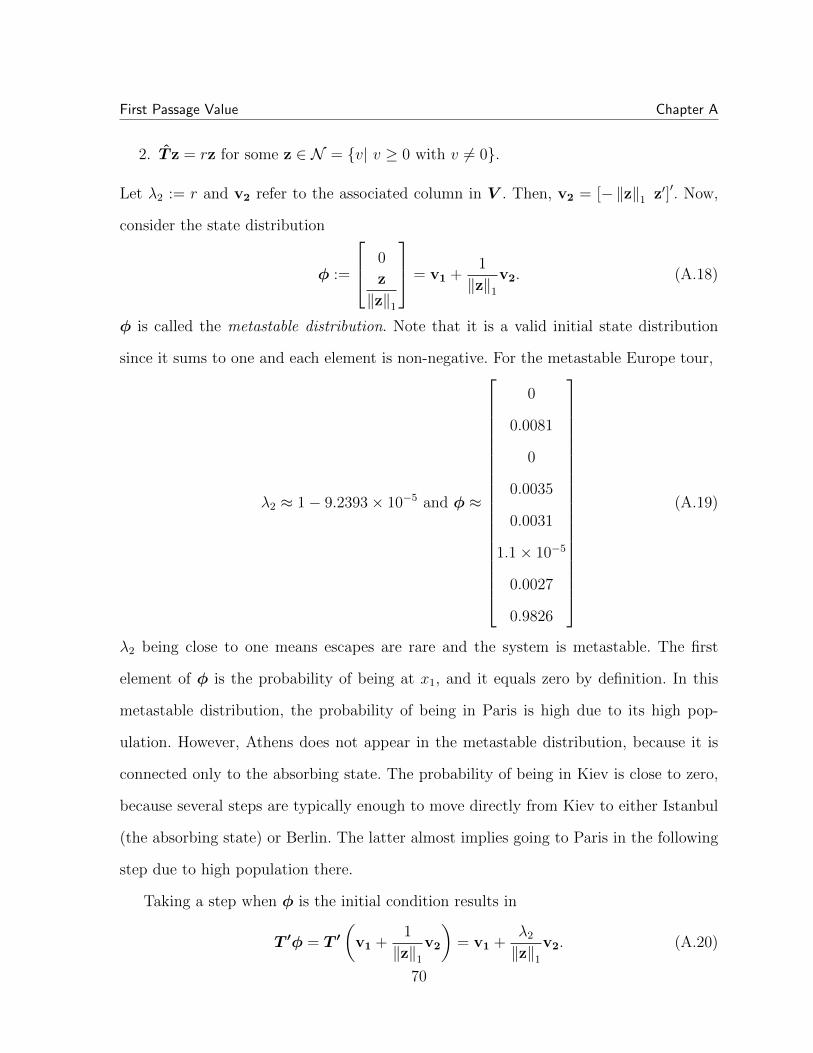
First Passage Value Chapter A
2. T z = rz for some z ∈ N = v| v ≥ 0 with v 6= 0.
Let λ2 := r and v2 refer to the associated column in V . Then, v2 = [−‖z‖1 z′]′. Now,
consider the state distribution
φ :=
0
z
‖z‖1
= v1 +1
‖z‖1
v2. (A.18)
φ is called the metastable distribution. Note that it is a valid initial state distribution
since it sums to one and each element is non-negative. For the metastable Europe tour,
λ2 ≈ 1− 9.2393× 10⁻⁵ and φ ≈
0
0.0081
0
0.0035
0.0031
1.1× 10⁻⁵
0.0027
0.9826
(A.19)
λ2 being close to one means escapes are rare and the system is metastable. The first
element of φ is the probability of being at x1, and it equals zero by definition. In this
metastable distribution, the probability of being in Paris is high due to its high pop-
ulation. However, Athens does not appear in the metastable distribution, because it is
connected only to the absorbing state. The probability of being in Kiev is close to zero,
because several steps are typically enough to move directly from Kiev to either Istanbul
(the absorbing state) or Berlin. The latter almost implies going to Paris in the following
step due to high population there.
Taking a step when φ is the initial condition results in
T ′φ = T ′(
v1 +1
‖z‖1
v2
)= v1 +
λ2
‖z‖1
v2. (A.20)
70

First Passage Value Chapter A
Naturally, the resulting distribution is also non-negative and sums to one. In addition,
the first component is
1 +λ2
‖z‖1
(−‖z‖1) = 1− λ2, (A.21)
which means the system escaped with probability 1− λ2. Furthermore, given the system
did not escape, φ is the final probability distribution for the states. This fact can be seen
by zeroing the first component of T ′φ and scaling to sum to one. So, when φ is the initial
state distribution, the probability of escaping is 1− λ2, the probability of staying in the
same distribution (φ) is λ2.
Now let the initial condition be φ, that is p[0] = φ. The expected number of steps
before escape corresponds to the term mean first passage time (MFPT) in [Byl and
Tedrake, 2009]. The higher MFPT is, the more stable a system is said to be. Two cases
are possible depending on the probability of taking a step: If λ2 = 1, then the probability
of escape is zero. In this case the system takes infinitely many steps without escaping to
the halt state. The other case (λ2 < 1) is relatively more complicated and interesting as
focused next.
A.2.1 System-wide First Passage Time
Given the probability of taking a step without escaping is λ2 < 1, the probability of
taking n steps only, equivalently escaping at the nth step is
Pr(X[n] = x1, X[n− 1] 6= x1) = λn−12 (1− λ2). (A.22)
Realize that as n → ∞, the right hand side goes to zero, which means the escape is
inevitable. The step ended up escaping also counts as a step, which can be verified
considering escaping at the first step (taking 1 step only). When n = 1 is substituted,
71

First Passage Value Chapter A
1− λ2 is obtained as expected. Then, the expected number of steps can be calculated as
MFPT = E[FPT]
=∞∑n=1
n Pr(X[n] = x1, X[n− 1] 6= x1)
=∞∑n=1
nλn−12 (1− λ2) =
1
1− λ2
,
(A.23)
where FPT stands for first passage time and the fact that λ2 < 1 is used. As a result,
MFPT can then be calculated using
M =
∞ λ2 = 1,
1
1− λ2
λ2 < 1.
(A.24)
The MFPT for the Europe tour is
M ≈ 10, 823. (A.25)
So, if p[0] = φ, then the system takes approximately 10,823 steps on average.
The standard deviation of FPT can be calculated by
E[FPT2] =∞∑n=1
n2 Pr(X[n] = x1, X[n− 1] 6= x1)
=∞∑n=1
n2λn−12 (1− λ2) =
1 + λ2
(1− λ2)2
=⇒√
E[FPT2]− (E[FPT])2 = M√λ2. (A.26)
Then for the Europe tour, the standard deviation of FPT is M√λ2 ≈ 10, 822. Note that
λ2 being close to one results in a standard deviation close to the mean.
The MFPT vector, m, gives the MFPT for each state and it is defined as
mi :=
0 i = 1,
1 +∑j
Tijmj otherwise.(A.27)
72

First Passage Value Chapter A
Equation (A.27) says it takes zero steps to go to the halt state if the system escaped
already. Otherwise, the number of steps until halt is 1 less after a step is taken. For the
Europe tour, the solution to (A.27) is
m ≈
0
10, 825
1
10, 652
10, 825
2, 121
10, 674
10, 824
. (A.28)
This vector says if the initial state is x2, then 10, 825 steps are expected before escape.
Note that London, Paris, Madrid, Berlin and Rome have MFPT close to the system-wide
MFPT M . Also the MFPT of Istanbul and Athens are very small. However, Kiev has a
MFPT that is not close to zero or the system-wide MFPT, because m1 = 0, m4 ≈ M ,
and
m6 = T61m1 + T64m4 + T66m6 (A.29)
implies
m6 ≈T64
1− T66
= 2, 153. (A.30)
For walking robots, the picture is the same. Metastable states are almost equally stable
(m2 ≈ m4 ≈ m5 ≈ m7 ≈ m8 ≈ M) and some states are doomed to fail (m3 = 1). Also
some states are risky and likely to fail in the next step, otherwise they are mapped to
the metastable region, just like Kiev. This structure is the case when memory constant,
which is to be defined shortly, is small.
73

First Passage Value Chapter A
By using (A.9), it is straightforward to obtain
m =
0
(I− T ′)−11
. (A.31)
(I − T ′) is invertible when λ2 < 1, which is the hidden assumption made while defining
the MFPT vector. The system-wide MFPT calculated in (A.23) can be also obtained by
M = m′φ =1
‖z‖1
[1 ... 1](I− T )−1z. (A.32)
This equivalence makes sense because each state has its own MFPT, and MFPT of the
metastable distribution is just a convex combination of each state’s MFPT weighted
according to φ. Indeed
M =1
‖z‖1
[1 ... 1](I− T )−1z
=1
‖z‖1
[1 ... 1](I− T )−1(I− T + T )z
=1
‖z‖1
[1 ... 1](I + (I− T )−1T )z
=1
‖z‖1
[1 ... 1]z +1
‖z‖1
[1 ... 1](I− T )−1T z
= 1 + λ21
‖z‖1
[1 ... 1](I− T )−1z
= 1 + λ2M =⇒ M = 1/(1− λ2) = M.
(A.33)
Note that M is upper bounded by the largest element in m. In fact, any initial state
distribution, p[0], has a MFPT that is a convex combination of the mi values.
MFPT of the metastable distribution is useful for various reasons. First of all, it is
a lower bound for average steps taken from at least one of the states, because it is a
convex combination of mis. So, there exists state(s) at least as stable. Secondly, it is a
meaningful and intuitive measure of overall stability. Often systems quickly converge to
their metastable distributions, where MFPT becomes the true value. Thirdly, system-
wide MFPT also has advantages over calculating the MFPT vector. In case T is large,
74
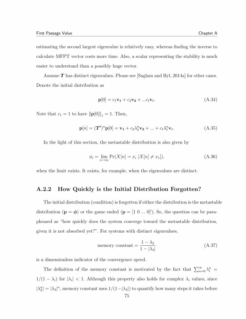
First Passage Value Chapter A
estimating the second largest eigenvalue is relatively easy, whereas finding the inverse to
calculate MFPT vector costs more time. Also, a scalar representing the stability is much
easier to understand than a possibly huge vector.
Assume T has distinct eigenvalues. Please see [Saglam and Byl, 2014a] for other cases.
Denote the initial distribution as
p[0] = c1v1 + c2v2 + ...c`v`. (A.34)
Note that c1 = 1 to have ‖p[0]‖1 = 1. Then,
p[n] = (T ′)np[0] = v1 + c2λn2v2 + ...+ c`λ
n` v`. (A.35)
In the light of this section, the metastable distribution is also given by
φi = limn→∞
Pr(X[n] = xi |X[n] 6= x1]), (A.36)
when the limit exists. It exists, for example, when the eigenvalues are distinct.
A.2.2 How Quickly is the Initial Distribution Forgotten?
The initial distribution (condition) is forgotten if either the distribution is the metastable
distribution (p = φ) or the game ended (p = [1 0 ... 0]′). So, the question can be para-
phrased as “how quickly does the system converge toward the metastable distribution,
given it is not absorbed yet?”. For systems with distinct eigenvalues,
memory constant =1− λ2
1− |λ3|(A.37)
is a dimensionless indicator of the convergence speed.
The definition of the memory constant is motivated by the fact that∑∞
n=0 λni =
1/(1 − λi) for |λi| < 1. Although this property also holds for complex λi values, since
|λn3 | = |λ3|n, memory constant uses 1/(1−|λ3|) to quantify how many steps it takes before
75

First Passage Value Chapter A
vanishing. Higher λ3 results in larger 1/(1 − |λ3|), which means the initial condition is
forgotten slower and more steps are required to forget the same amount of initial condition
information. λ3 gives the worst case scenario, so the memory constant is a conservative
value. (1/(1− |λ3|) is divided by M = 1/(1− λ2) for a relative memory constant, which
is upper bounded by 1.
Note that the memory constant being smaller than ε implies M > 1/ε. Thus, small
memory constants require metastability. If, on the other hand, the memory constant is
very close to one, then there is another mode almost as stable as the one associated with
λ2. In such cases it may be useful to use the next |λi| instead of |λ3|, until a small memory
constant is obtained. In particular, when the eigenvalues are not necessarily distinct, it
might be the case that λ2 = |λ3|.
For the Europe tour example, the memory constant is 1.1688 × 10⁻⁴. This small
memory constant indicates the structure mentioned earlier, where there are metastable
states, controllable unreachable states, doomed states, risky states, and halt state. Some
other motivating applications of MFPT calculation is presented later in this Chapter.
A.3 Mean First Passage Value
Calculating the discrete time to a state of interest has potential to be greatly useful,
but in some applications, metrics other than expected number of steps before absorption
are of interest. To illustrate, instead of how many decisions it took before reaching Istan-
bul, travel-time or distance to Istanbul might be needed. For this matter, MFPT can be
generalized as mean first passage value (MFPV), where “value” depends on the task, for
example, mean first passage distance. So, MFPT is a special case of MFPV, where value
is discrete time steps.
76

First Passage Value Chapter A
Redefining m from (A.27) as the MFPV vector gives the MFPV for each state as
mi :=
0 i = 1∑j
TijRij +∑j
Tijmj otherwise,(A.38)
where Rij is the reward (value) of transitioning from state xi to xj. Then, vector m can
be calculated as
m =
0
(I− T ′)−1
∑j
T2jR2j
.
.
.∑j
T`jR`j
. (A.39)
And the (system-wide) MFPV is
M = m′φ. (A.40)
For the metastable Europe tour example, consider the information provided in Ta-
ble A.1. Then, using (A.40) mean first passage distance can be calculated to be 325.68
thousand km. This calculation is achieved by setting, for example, R24 = 1, 098 km,
which corresponds to the distance between London, and Berlin.
77

First Passage Value Chapter A
Time (h:m) Distance (km)
London (2) - Paris (8) 5:06 454
London (2) - Berlin (4) 10:25 1,098
Madrid (5) - Paris (8) 11:10 1,270
Rome (7) - Paris (8) 12:46 1,419
Berlin (4) - Paris (8) 9:18 1,055
Berlin (4) - Kiev (6) 14:41 1,329
Berlin (4) - Istanbul (1) 21:39 2,210
Kiev (6) - Istanbul (1) 19:00 1,459
Rome (7) - Istanbul (1) 22:46 2,262
Athens (3) - Istanbul (1) 11:13 1,095
Table A.1: Travel times and distances for the roads of Europe map in Figure A.1.For the game explained in that figure’s caption, the values in this table are used tocalculate the expected distance and time before visiting Istanbul.
The travel-time only (excluding the days spent in a city) is calculated by setting
Rii = 0. Then, it takes 128 days on average before Istanbul. The MFPV vector for this
case is
m =
0
128.4756
0.4674
126.6098
128.7334
25.9478
127.0149
128.2681
days. (A.41)
78

First Passage Value Chapter A
Remember that a random decision is made after spending a day in the city. For the
MFPV calculation, to include those days spent in a city, the reward needs to be set such
that Rii = 1 day. This setting results in a MFPV of 29 years, which is much higher
than 128 days. One reason of this difference is because once in Paris, there is a 0.9825
probability to stay in Paris.
In addition, MFPV does not need to have a physical meaning. Multiple objectives
can be included in a single value function, for example for walking robots failure events,
such as falling down, can be penalized while also rewarding fast speed and low energy
use. The value, or the cost function, does not need to have a physical correspondence.
Number of steps minus 10−3 times energy consumption is a valid value definition. Please
see [Saglam and Byl, 2014b] for further details and usage of this example.
A.4 Confidence Levels on Value
In some applications, instead of the mean FPV, a conservative FPV bound for a
particular “confidence level” pr is needed. In other words, a value above lower first passage
time (LFPT) would be observed with probability pr, and a value below upper first passage
time (UFPT) would be observed with probability pr.
A.4.1 First Passage Time
The probability of taking more than LFPT steps is λLFPT2 . Then, the lower bound on
number of steps taken with probability pr can be calculated by
LFPT(pr) = logλ2pr. (A.42)
Note that LFPT(1)=0, so taking only a single step is guaranteed, which leads to the halt
state. The probability of taking less than UFPT steps is 1 − λUFPT−12 . Then, the upper
79

First Passage Value Chapter A
bound on number of steps taken with probability pr is
UFPT(pr) = logλ2(1− pr) + 1. (A.43)
Since limpr→1
UFPT(pr) = ∞, it may theoretically take infinitely many steps before con-
verging to the halt state. Then FPT can be limited for a given probability as
LFPT ≤ FPT ≤ UFPT. (A.44)
Having LFPT<UFPT requires pr > λ2/(1 + λ2), where right hand side equals 0.5 for
λ2 = 1. To illustrate the advantage of looking to FPT, consider the metastable Europe
tour example. The probability of the journey taking more than M = 10, 823 days is only
36.79 %. On the other hand,
1, 140 ≤ FPT(0.9) ≤ 24, 921,
108 ≤ FPT(0.99) ≤ 49, 842.
(A.45)
These numbers are not coincidence. As λ2 → 1, the probability of taking M steps is
limλ2→1
λ1/(1−λ2)2 =
1
e≈ 0.3679. (A.46)
In fact, 0.3679 is an upper limit for the probability of taking 1/(1− λ2) steps for any λ2.
In addition, when λ2 and pr are close to one,
LFPT(pr) =ln(pr)
ln(λ2)≈ 1− pr
1− λ2
= (1− pr)M, (A.47)
UFPT(pr) =ln(1− pr)ln(λ2)
+ 1 ≈ −ln(1− pr)M, (A.48)
where M denotes MFPT.
LFPT is of interest for walking systems, to give a conservative bound on steps to
failure, while UFPT would be helpful in modeling epidemics, to obtain a conservative
time when everyone is healthy, which means recurrence to an “all-healthy” system state.
80

First Passage Value Chapter A
A.4.2 First Passage Value
Using MFPT and MFPV value per step can be used to write
FPV =MFPV
MFPTFPT, (A.49)
where FPV denotes first passage value. When the value is the distance in the metastable
Europe tour example,
3.4× 10⁴ ≤ FPV(0.9) ≤ 7.5× 10⁵,
3.2× 10³ ≤ FPV(0.99) ≤ 1.5× 10⁶.
(A.50)
So, with probability 0.99, the journey takes more than 3.2 thousand or less than 1.5
million kilometers.
A.5 Controlling the Europe Tour
In order to control a system, a goal is needed. For instance, going to Istanbul as
quickly as possible could be a goal for the Europe tour. It is then useful to quantify the
performance toward achieving that goal. For example, number of days before reaching
Istanbul would be a meaningful metric to minimize. FPV analysis provides useful metrics
for many applications. To illustrate, the more steps a walking robot takes before failure,
the more stable it is said to be. Once the performance is quantified, the control can be
optimized.
Control action comes into play in two ways: Low-level and high-level. For the Europe
tour, say the probability for city change is directly proportional to population to the
power k, e.g.,
Probability of staying in Madrid =(Population of Madird)k
(Population of Madird)k + (Population of Paris)k,
(A.51)
81
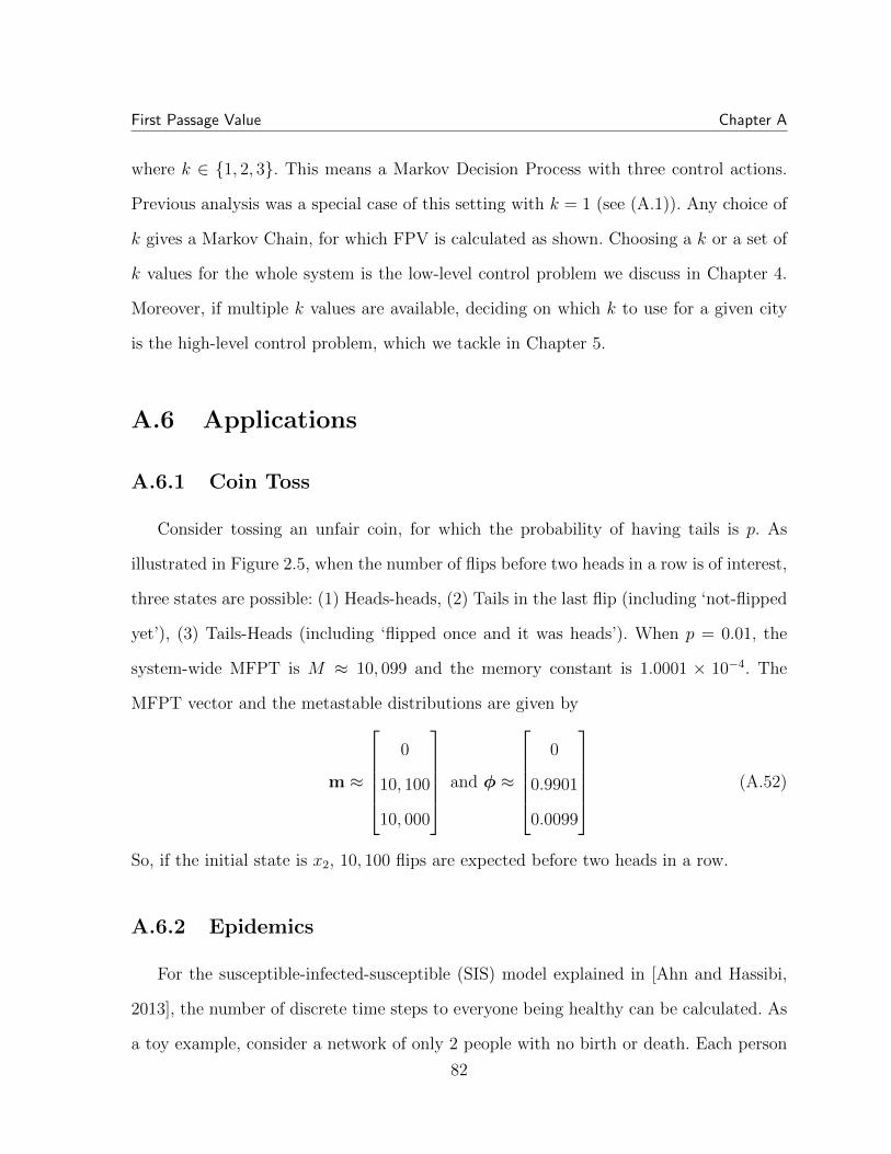
First Passage Value Chapter A
where k ∈ 1, 2, 3. This means a Markov Decision Process with three control actions.
Previous analysis was a special case of this setting with k = 1 (see (A.1)). Any choice of
k gives a Markov Chain, for which FPV is calculated as shown. Choosing a k or a set of
k values for the whole system is the low-level control problem we discuss in Chapter 4.
Moreover, if multiple k values are available, deciding on which k to use for a given city
is the high-level control problem, which we tackle in Chapter 5.
A.6 Applications
A.6.1 Coin Toss
Consider tossing an unfair coin, for which the probability of having tails is p. As
illustrated in Figure 2.5, when the number of flips before two heads in a row is of interest,
three states are possible: (1) Heads-heads, (2) Tails in the last flip (including ‘not-flipped
yet’), (3) Tails-Heads (including ‘flipped once and it was heads’). When p = 0.01, the
system-wide MFPT is M ≈ 10, 099 and the memory constant is 1.0001 × 10⁻⁴. The
MFPT vector and the metastable distributions are given by
m ≈
0
10, 100
10, 000
and φ ≈
0
0.9901
0.0099
(A.52)
So, if the initial state is x2, 10, 100 flips are expected before two heads in a row.
A.6.2 Epidemics
For the susceptible-infected-susceptible (SIS) model explained in [Ahn and Hassibi,
2013], the number of discrete time steps to everyone being healthy can be calculated. As
a toy example, consider a network of only 2 people with no birth or death. Each person
82

First Passage Value Chapter A
is either susceptible or infected, so four states are possible as listed in Table A.2. Note
that when both patients are susceptible (State 1), the state does not change, because
noone can become infected.
State 1 State 2 State 3 State 4
Patient 1 Susceptible Susceptible Infected Infected
Patient 2 Susceptible Infected Susceptible Infected
Table A.2: Possible states for SIS model of epidemics with 2 people
Let ‘the probability of recovery when a node is infected’ be δ = 0.01, and ‘the prob-
ability to be infected when the other node is infected’ be β = 0.8. Then, the stochastic
matrix is given by
T =
1 0 0 0
(1− β)δ (1− δ)(1− β) βδ β(1− δ)
(1− β)δ βδ (1− δ)(1− β) β(1− δ)
δδ δ(1− δ) δ(1− δ) (1− δ)(1− δ)
=
1 0 0 0
0.002 0.198 0.008 0.792
0.002 0.008 0.198 0.792
0.001 0.0099 0.0099 0.9801
.
(A.53)
λ2 is such that MFPT is M = 6.8383 × 10³. In addition, λ3 = 0.19, and the memory
83

First Passage Value Chapter A
constant is 1.8× 10⁻⁴. The MFPT vector and the metastable distribution are given by
m ≈
0
6822.7
6822.7
6838.7
and φ ≈
0
0.0122
0.0122
0.9757
. (A.54)
Small memory constant results in states having a MFPT close to either zero or M . It is
interesting to see that with a high probability (0.9757), both people are infected during
the epidemic while all healthy state is the stable one.
Estimating survival times of epidemic spreads can potentially be useful for public
health research to optimize actions while minimizing deaths and expenditures.
A.6.3 Driving a Car
Arguably, given enough time (millions of years if necessary), any driver will be in-
volved in an accident. The same is true for autonomous cars including the Google car.
The expected miles driven between accidents can be estimated to quantify and increase
the safety.
A.6.4 Queueing and Polling Systems - Traffic Intersection
Queueing theory deals with waiting lines and queues. One application of polling sys-
tems, which are extensions of queueing systems, is traffic intersections with multiple lines
as illustrated in [Miculescu and Karaman, 2014]. As a toy example, consider the intersec-
tion with two lines shown in Figure A.2. The goal of the traffic light of the intersection is
to avoid traffic jam, which is defined as having more than 4 cars in a lane. Assume that
each turn a single car may pass through the intersection and new cars come stochastically
to each line. Let the number of cars arriving at each lane have Poisson distribution with
84

First Passage Value Chapter A
parameter λ = 0.1. This intersection can be easily treated as a Markov Decision Process.
If the controller always allows the same line to proceed, the expected discrete-time to
traffic jam is around 10. The exhaustive policy allows a line to proceed until that line
is empty and then switches to the other lane. This policy results with 1.09 × 10⁶ turns
before traffic jam.
Figure A.2: An intersection with two lanes. Cars are either going from west to east orsouth to north. Blue cars are waiting to pass through the intersection. Cyan coloredcar recently moved to the north side of the intersection. The arrow shows which laneis allowed to proceed. In this toy example, traffic jam corresponds to 5 or more cars ina lane. The goal of the traffic lights is to minimize the traffic jam rates. Each turn asingle car may pass through the intersection and new cars come stochastically to eachline. The number of cars arriving at each lane has Poisson distribution with parameterλ = 0.1. This intersection can be easily treated as a Markov Decision Process.
85

First Passage Value Chapter A
A.7 Conclusion
This appendix studied first passage time, which is a survival metric. It presented
system-wide mean first passage time (MFPT), which is calculated using the second
largest eigenvalue of the stochastic transition matrix. The chapter also illustrated that
for metastable systems, system-wide MFPT is an accurate indicator across a large set
of states of those frequently visited. Then mean first passage value (MFPV) was intro-
duced, which gives a more general value of interest, such as energy expenditure, distance,
or time. Bounds on first passage value (FPV) was provided for a given confidence level.
The chapter also showed how these tools explained can be used to low-level and high-level
control hybrid systems.
86

Appendix B
Biped Model
The methods of this paper are appropriate and useful for various systems. To show
applicability to high degree of freedom (DOF) robots (compared to 2-link walker in [Byl
and Tedrake, 2009] and 3-link walker of [Chen and Byl, 2012]), the analysis in this thesis
is carried out with the 5-link biped shown in Figure B.1. The model is based on the
RABBIT robot shown in Figure 1.4c [Chevallereau et al., 2003].
RABBIT has point feet, 5 degrees-of-freedom (DOF) and four actuators located at
the internal joints. Since the robot cannot produce ankle torques, it is underactuated
by 1 DOF. While studying RABBIT, we restrict our attention to planar motion and
assume links are rigid. The angles shown in the figure form q := [q1 q2 q3 q4 q5]T , the
ten dimensional state of the robot is defined as x := [qT qT ]T , and sh denotes the height
of the swing foot. The model parameters are taken from RABBIT [Westervelt et al.,
2007] and listed in Table B.1.
Depending on the number of legs in contact with the ground, the robot is either in
the single or double support phase. Walking consists of these two phases in sequence. The
single support (swing) phase has continuous dynamics. Using a Lagrangian approach, the
87

Biped Model Chapter B
Table B.1: Model parameters for the five-link robot based on RABBIT [Westerveltet al., 2007]
Description Parameter Label Value
Torso Mass mT 12 kg
Femur Mass mf 6.8 kg
Tip Mass mt 3.2 kg
Torso Inertia IT 1.33 kg m2
Femur Inertia If 0.47 kg m2
Tip Inertia It 0.20 kg m2
Torso Length lT 0.63 m
Femur Length lf 0.4 m
Tip Length lt 0.4 m
Torso Mass Center pT 0.24 m
Femur Mass Center pf 0.11 m
Tip Mass Center pt 0.24 m
Gravitational Acceleration g0 9.81 m/s2
Gear Ratio ng 50
Ground Friction Coefficient µs 0.6
Saturation Limit usat 50 Nm
88

Biped Model Chapter B
q5
q1q2
−q3−q4
Torso
Swing Femur
Swing Tip
Swing Leg
Stance Leg
sh
lTpT
lfpf
lt pt
Figure B.1: Illustration of the five-link robot with identical legs that is used as ourbiped model in this thesis. This model is based on RABBIT shown in Figure 1.4c.
equations of motion can be derived in the canonical form of
D(q)q + C(q, q)q +G(q) = Bu, (B.1)
where u is the input. An important point is that q consists of the five angles depicted in
Fig. B.1 whereas u has only four elements. The system has this degree of underactuation
because of the passive joint at the stance tip. The swing dynamics can be equivalently
expressed as
x =
q
D−1(−Cq −G+Bu)
=: f(x) + g(x)u. (B.2)
During the swing phase of a successful step, the swing leg takes off from the ground,
passes the stance leg and lands on a further point on the ground. So, each single support
phase starts and ends with double support phases. As the robot has point feet, the double
support (stance) phase can be well captured as an instantaneous impact event. The robot
experiences this impact whenever the swing foot hits the ground (sh = 0) from above
89

Biped Model Chapter B
(sh < 0). Let us denote this impact surface, aka the jump set, by S. Then we have
x+ = ∆(x−) :=
∆q q−
∆q(q−) q−
x ∈ S, (B.3)
where x− = [(q−)T (q−)T ]T and x+ are the states just before and after the impact re-
spectively. Conservation of energy and the principle of virtual work gives the mapping
∆ [Westervelt et al., 2007], [Hurmuzlu and Marghitu, 1994]. Essentially, this model as-
sumes instantaneous, inelastic collisions between the swing leg tip and the ground, with
instantaneous changes in velocities to reflect the effects of impulsive forces exerted on
the robot.
Although the robot’s position and orientation do not actually change according to
the impact model, we relabel the legs every step, so the previous swing leg becomes the
new stance leg and vice versa. So, ∆q is such that we have ∆q[q1 q2 q3 q4 q5]T =
[q2 q1 q4 q3 q5]T . Without relabeling, a periodic walking gait would have two steps as
its period.
Since a step consists of a single support phase and an impact event, it has hybrid
dynamics as illustrated in Figure B.2. In our modeling, we assume the impact event
occurs first, but the order in the definition of a step is an arbitrary choice, so long as
one remains consistent after deciding. As seen in Figure B.2, for a step to be successful,
certain “validity conditions” must be satisfied, which we list next. After impact, the
former stance leg must lift from ground with no further interaction with the ground until
the next impact. Also, the swing foot must have progressed past the stance foot before
the impact of the next step occurs. Only the feet should contact the ground. Furthermore,
the force on the stance tip during the swing phase, and the force on the swing tip at the
impact should satisfy the friction constraint given by
Ffriction = Fnormal µs > |Ftransversal|. (B.4)
90

Biped Model Chapter B
If validity conditions are not met, the step is labeled as “unsuccessful” and the system
is modeled as transitioning to a failure state. This is a conservative model, because in
reality violating these conditions does not necessarily mean failure.
x = f(x) + g(x)u
x+ = ∆(x)
Swing tip touched the groundand validity conditions
are not violated
Validity conditionsare violated
Failure
Figure B.2: Hybrid model of a step and the failure state. Swing phase is governed bycontinuous dynamics or flows, which are interrupted by discontinuous impacts.Image inspired by [Westervelt et al., 2007].
91

Appendix C
Modeling Rough Terrain
To study rough terrain walking, the methodology in Chapter 2 assumes stochastically
changing terrain, which requires modeling ground with finitely many dimensions. Two
most elementary models, which are only one dimensional disturbances to the robot, are
presented in Figure C.1. This thesis mainly assumes sloped terrain model, but results
when heights are varying instead are also presented in Section 4.3.
slope
(a) Sloped Terrain
stepheight
(b) Step Terrain
Figure C.1: One dimensional terrain disturbances
92

Modeling Rough Terrain Chapter C
A natural concern is related to the validity of these terrain models. Consider the higher
dimensional terrain disturbance in Figure C.2. Red dashed line shows the trajectory of
the swing foot for a specific initial condition and the controller employed. Given this
trajectory, all three terrains shown on the right hand side of Figure C.2 are equivalent
to the original terrain. In particular, the terrain in the right bottom is generated with
double-sloped terrain model. In addition to the sloped terrain of Figure C.1a, this model
has an extra dimension which stores the slope experienced at impact. Adopting double-
sloped terrain is a topic of future work.
Equivalent Terrains
Figure C.2: Higher dimensional terrain disturbances
93

Appendix D
Extended Hybrid Zero Dynamics
Any one of the numerous control schemes proposed for bipedal locomotion can be opti-
mized and benchmarked using the methods presented in this thesis. As case demonstra-
tion, we illustrate our results mainly on the extended hybrid zero dynamics framework
explained in this Appendix.
In the literature of bipedal locomotion control, typically time trajectories are imposed
to achieve a desired walking motion. However, time-invariant controllers have critical
advantages over their time-varying counterparts. For example, imagine someone holding
the robot in the mid-step for a second. After released, instead of hurrying to catch up
the time trajectories for re-synchronization, the robot better continue the interrupted
motion. For this reason, defining an internal clock which defines how far the robot is
at a step is a meaningful approach, which has led to the hybrid zero dynamics (HZD)
framework [Westervelt et al., 2003]. The controller scheme introduced in this thesis is
a generalization of the now-famous HZD control in two-ways. First, we modify it for
non-flat terrain as in [Yadukumar et al., 2012] and [Saglam and Byl, 2015]. Secondly,
and much more importantly, HZD controllers assume deterministic terrain by design,
where the internal clock ticks from 0 to 1 at every step. In this thesis, we extend the
94
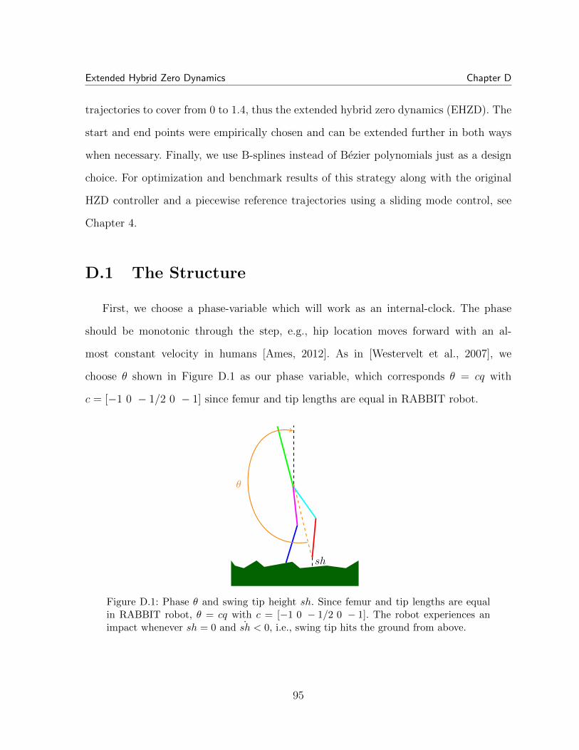
Extended Hybrid Zero Dynamics Chapter D
trajectories to cover from 0 to 1.4, thus the extended hybrid zero dynamics (EHZD). The
start and end points were empirically chosen and can be extended further in both ways
when necessary. Finally, we use B-splines instead of Bezier polynomials just as a design
choice. For optimization and benchmark results of this strategy along with the original
HZD controller and a piecewise reference trajectories using a sliding mode control, see
Chapter 4.
D.1 The Structure
First, we choose a phase-variable which will work as an internal-clock. The phase
should be monotonic through the step, e.g., hip location moves forward with an al-
most constant velocity in humans [Ames, 2012]. As in [Westervelt et al., 2007], we
choose θ shown in Figure D.1 as our phase variable, which corresponds θ = cq with
c = [−1 0 − 1/2 0 − 1] since femur and tip lengths are equal in RABBIT robot.
sh
θ
Figure D.1: Phase θ and swing tip height sh. Since femur and tip lengths are equalin RABBIT robot, θ = cq with c = [−1 0 − 1/2 0 − 1]. The robot experiences animpact whenever sh = 0 and sh < 0, i.e., swing tip hits the ground from above.
95

Extended Hybrid Zero Dynamics Chapter D
Second, we decide on four independent variables to control h0 because the robot has
four actuators only. It is intuitive to control the relative (internal) angles, i.e., h0 :=
[q1 q2 q2 q3 q4]T . Then h0 is in the form of h0 = H0 q, where H0 = [I4 0]. Changing h0
later is an easy step in this framework and it does not affect the performance to the
author’s experience.
Third, let hd(θ) be the references for h0. Then the tracking error is given by
h(q) := h0(q)− hd(θ) = H0q − hd(cq). (D.1)
Taking the first derivative with respect to time yields
h =∂h
∂xx =
∂h
∂xf(x) =: Lfh = 〈∇h, f〉 , (D.2)
where we used the fact that∂h
∂xg(x) = 0. For the clarity of later equations, we will use
the Lie derivative (L) notation. Then, we have
h = L2fh+ LgLfh u. (D.3)
Substituting the linearizing controller structure
u = (LgLfh)−1(−L2fh+ v) (D.4)
to (D.3) yields
h = v. (D.5)
There are various methods to design v in (D.4) to force h (and h) to zero [Ames et al.,
2012]. While even a PD controller could be sufficient, a sliding mode control (SMC) is
preferable, due to its finite time convergence [Sabanovic and Ohnishi, 2011], which we
summarize next.
96

Extended Hybrid Zero Dynamics Chapter D
D.2 Sliding Mode Control
Remember that h corresponds to tracking error. The generalized error is defined as
σi = hi + hi/τi, i = 1, 2, 3, 4, (D.6)
where τis are time constants for hi. Note that when the generalized error is driven to
zero, i.e. σi = 0, we have
0 = hi + hi/τi. (D.7)
The solution to this equation is given by
hi(t) = hi(t0) exp(−(t− t0)/τi), (D.8)
which drives hi to 0 exponentially fast. Finally, v in (D.4) is given by
vi = −ki|σi|2αi−1sign(σi), i = 1, 2, 3, 4, (D.9)
where ki > 0 and 0.5 < αi < 1 are called the convergence coefficient and convergence
exponent respectively. Note that if we had αi = 1, this would simply be a standard PD
controller. Then, ki/τi and ki are analogous to the proportional and derivative gains of
a PD controller. However, 0.5 < αi < 1 ensures finite time convergence. In this thesis we
used αi = 0.75, τi = 0.1, ki = 10 for all controllers, but hd was different for each low-level
controller.
What the controller does is driving the system to the “zero dynamics manifold”,
noted by Z, where h = 0 and h = 0. The following two sections consider the dynamics
on this manifold. The final goal is to design hd such that the desired walking motion is
generated.
97

Extended Hybrid Zero Dynamics Chapter D
D.3 Swing Phase Zero Dynamics
Let V be the potential energy of the robot, γ0(q) be the last row of D and define
γ := γ0q. Then, Lgγ = 0 and Lfγ = −∂V∂q5
∣∣∣∣Z
. For x ∈ Z we transform coordinates by
ξ1 = θ, ξ2 = γ, (D.10)
to equivalently express the system dynamics during the swing phase as
ξ1 = cq, ξ2 = Lfγ, (D.11)
where the right-hand sides are evaluated at
q = H−1
hdξ1
(because ξ1 = θ = cq and H0q = h0 = hd for x ∈ Z),
and q =
∂h∂qγ0
−1 0
ξ2
(because h = 0 for x ∈ Z and ξ2 = γ = γ0q).
(D.12)
To evaluate q, we can alternatively differentiate q from above to get
q = H−1
∂hd∂θ1
θ (D.13)
Using (D.12) we can write (D.11) as
ξ1 = κ1(ξ1)ξ2, ξ2 = κ2(ξ1). (D.14)
98

Extended Hybrid Zero Dynamics Chapter D
D.4 Hybrid Zero Dynamics Impact
As we will see, hd will be designed such that x− ∈ Z implies x+ ∈ Z. Now assume
the swing foot passed the stance foot and had an impact. Let q−0 denote the angles just
before the impact on hd. Then, q−0 is a solution toh(q)
sh
= 0, (D.15)
where sh is the swing tip height as drawn in Figure D.1. At the impact, the angles
are relabeled as in (B.3). So, after the impact we have q+0 = ∆qq
−0 . The phases at the
beginning and end of the step are simply θ+ := cq+0 and θ− := cq−0 respectively.
Similarly let q−0 and q+0 denote the velocities just before and after the impact respec-
tively. ξ−2 and ξ+2 are the corresponding ξ2 values. Then, using (D.12) we get
q−0 =
∂h∂q (q−0 )
γ0(q−0 )
−1 0
1
ξ−2 =: λq ξ−2 (D.16)
From (B.3), we obtain q+0 = ∆q(q
−0 ) q−0 and ξ+
2 = γ0(q+0 ) q+
0 . Defining
δzero := γ0(q+0 ) ∆q(q
−0 ) λq, (D.17)
the impact map on zero dynamics manifold is given by
ξ+1 = θ+, ξ+
2 = δzero ξ−2 . (D.18)
D.5 Poincare Analysis
We then define a Poincare section just before the impact. We already know the angles
are q−0 . To find the fixed point on this Poincre map (if it exists), we also need a fixed
99

Extended Hybrid Zero Dynamics Chapter D
ξ−2 . Define ξ2b := ξ22/2. ξ+
2b and ξ−2b denote its value at the beginning and end of the step
respectively. Then, we have
dξ2b
dξ1
=κ2(ξ1)
κ1(ξ1). (D.19)
Integration over a step gives
ξ−2b − ξ+2b =
∫ θ−
θ+
κ2(ξ1)
κ1(ξ1)dξ1. (D.20)
Since impact maps ξ2b to δ2zeroξ2b, the fixed point ξ∗2b is obtained by solving
ξ∗2b − δ2zeroξ
∗2b =
∫ θ−
θ+
κ2(ξ1)
κ1(ξ1)dξ1. (D.21)
Then, the fixed points for the zero dynamics are
ξ∗1 = θ−, ξ∗2 =
√−2
1− δ2zero
∫ θ−
θ+
κ2(ξ1)
κ1(ξ1)dξ1. (D.22)
D.6 Under deterministic conditions
[Westervelt et al., 2007] carries a Poincare analysis, where the stability is formulated
analytically and shown numerically. Using the fixed point as initial condition, they simu-
late the 2D dynamics described in (D.11) until θ = θ− and calculate the steady-state cost
of transport (COT) defined in (4.1). However, we demonstrate in Figure 4.1 that opti-
mizing for energy efficiency results in sensitivity to perturbations, thus poor performance
on rough terrain.
During optimization, [Westervelt et al., 2003] impose many constraints such as fric-
tion violations and torque saturation limits. On the other hand, our method deals with
stochastic conditions to maximize global stability and no constraints are necessary for
optimization because it considers the full dynamics where, for example, the controller
can hit the saturation limit.
100

Extended Hybrid Zero Dynamics Chapter D
D.7 Reference Design
While forming trajectories in phase instead of time, we first scale and shift θ to have
an internal clock which ticks from 0 to 1 on the limit cycle using
τ(q) :=θ(q)− θ+
θ− − θ+. (D.23)
Then, the reference trajectory is determined as
hd(θ) :=
b1(τ)
b2(τ)
b3(τ)
b4(τ)
. (D.24)
To form trajectories defined by bj(τ)s, we use B-splines as formulated in [Patrikalakis
and Maekawa, 2010]. Each of the four trajectories is then defined as a linear combination
of control points αji and B-spline basis functions Ni,k(τ) given by
bj(τ) =n∑i=0
αjiNi,k(τ), n ≥ k − 1, τ ∈ [τk−1, τn+1], (D.25)
where k is order of the curve and the number of control points equals n + 1. The basis
functions Ni,k(τ) are uniquely determined by the knot vector
T = (τ0, τ1, ..., τk−1, τk, τk+1, ..., τn−1, τn, τn+1, ..., τn+k), (D.26)
which consist of n+ k + 1 elements. We use 4th order curves on the knot vector
T = (0, 0, 0, 0, 0.2, 0.4, 0.6, 0.8, 1, 1.2, 1.4, 1.4, 1.4, 1.4). (D.27)
The resulting 10 basis functions and their derivatives are pictured in Figure D.2.
10 basis functions imply 10 control points for each of the 4 bj(τ)s. So, 10 × 4 = 40
αji parameters need to be optimized. However, we demand hybrid invariance, so x− ∈ Z101

Extended Hybrid Zero Dynamics Chapter D
0 0.2 0.4 0.6 0.8 1 1.2 1.40
0.2
0.4
0.6
0.8
1
B0,4
B1,4 B2,4
B3,4 B4,4 B5,4 B6,4B7,4 B8,4
B9,4
τ0 τ4 τ5 τ6 τ7 τ8 τ9 τ13
τ1
τ2
τ3
τ10
τ11
τ12
(a) Basis functions
0 0.2 0.4 0.6 0.8 1 1.2 1.4−15
−10
−5
0
5
10
15
B0,4
B1,4
B2,4 B3,4 B4,4 B5,4 B6,4 B7,4
B9,4
B8,4
(b) Derivatives of basis functions
Figure D.2: 10 basis functions of order 4 with uniform knot vector in (D.27) and theirderivatives. On the limit cycle, the internal clock ticks from τ = 0 to τ = 1. We extendthe knots until τ = 1.4 for impacts on uneven terrain.
102
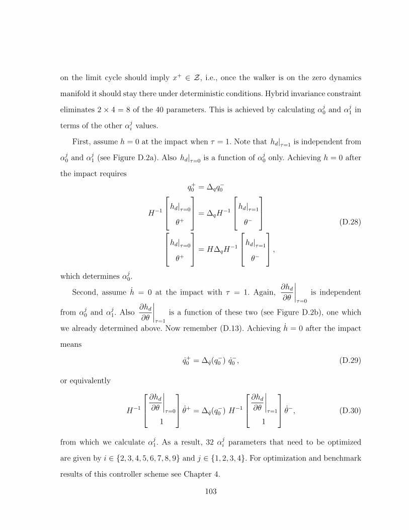
on the limit cycle should imply x+ ∈ Z, i.e., once the walker is on the zero dynamics
manifold it should stay there under deterministic conditions. Hybrid invariance constraint
eliminates 2 × 4 = 8 of the 40 parameters. This is achieved by calculating αj0 and αj1 in
terms of the other αji values.
First, assume h = 0 at the impact when τ = 1. Note that hd|τ=1 is independent from
αj0 and αj1 (see Figure D.2a). Also hd|τ=0 is a function of αj0 only. Achieving h = 0 after
the impact requires
q+0 = ∆qq
−0
H−1
hd|τ=0
θ+
= ∆qH−1
hd|τ=1
θ−
hd|τ=0
θ+
= H∆qH−1
hd|τ=1
θ−
,(D.28)
which determines αj0.
Second, assume h = 0 at the impact with τ = 1. Again,∂hd∂θ
∣∣∣∣τ=0
is independent
from αj0 and αj1. Also∂hd∂θ
∣∣∣∣τ=1
is a function of these two (see Figure D.2b), one which
we already determined above. Now remember (D.13). Achieving h = 0 after the impact
means
q+0 = ∆q(q
−0 ) q−0 , (D.29)
or equivalently
H−1
∂hd∂θ∣∣∣∣τ=0
1
θ+ = ∆q(q−0 ) H−1
∂hd∂θ∣∣∣∣τ=1
1
θ−, (D.30)
from which we calculate αj1. As a result, 32 αji parameters that need to be optimized
are given by i ∈ 2, 3, 4, 5, 6, 7, 8, 9 and j ∈ 1, 2, 3, 4. For optimization and benchmark
results of this controller scheme see Chapter 4.
103

Bibliography
[Abbel, 2012] Abbel, P. (2012). Discretization. In CS 287: Advanced Robotics LectureNotes. Accessed: 2015-05-06. Available from: http://www.cs.berkeley.edu/∼pabbeel/cs287-fa12/slides/discretization.pdf.
[Ahn and Hassibi, 2013] Ahn, H. J. and Hassibi, B. (2013). Global dynamics of epidemicspread over complex networks. In 2013 IEEE 52nd Annual Conference on Decisionand Control (CDC), pages 4579–4585.
[Ames et al., 2012] Ames, A., Galloway, K., and Grizzle, J. (2012). Control lyapunovfunctions and hybrid zero dynamics. In 2012 IEEE 51st Annual Conference on Decisionand Control (CDC), pages 6837–6842.
[Ames, 2012] Ames, A. D. (2012). First Steps toward Automatically Generating BipedalRobotic Walking from Human Data. In Robot Motion and Control 2011, number 422in Lecture Notes in Control and Information Sciences, pages 89–116. Springer London.Available from: http://link.springer.com/chapter/10.1007/978-1-4471-2343-9 8.
[Belle, 2008] Belle, G. v. (2008). Statistical Rules of Thumb. Wiley-Interscience, Hobo-ken, N.J, 2nd edition edition.
[Bellman, 1957] Bellman, R. (1957). A Markovian decision process. Indiana UniversityMathematics Journal, 6(4):679–684. Available from: http://www.iumj.indiana.edu/IUMJ/FULLTEXT/1957/6/56038.
[Benallegue and Laumond, 2013] Benallegue, M. and Laumond, J.-P. (2013). Metasta-bility for High-Dimensional Walking Systems on Stochastically Rough Terrain. InRobotics: Science and Systems.
[Bhounsule, 2014] Bhounsule, P. A. (2014). Numerical accuracy of two benchmark mod-els of walking: the rimless spoked wheel and the simplest walker. Dynamics of Contin-uous, Discrete and Impulsive Systems Series B: Applications and Algorithms, 21:137–148. Available from: http://engineering.utsa.edu/∼pab/pdw benchmark.pdf.
[Bhounsule et al., 2014] Bhounsule, P. A., Cortell, J., Grewal, A., Hendriksen, B.,Karssen, J. G. D., Paul, C., and Ruina, A. (2014). Low-bandwidth reflex-based
104
control for lower power walking: 65 km on a single battery charge. The Inter-national Journal of Robotics Research, page 0278364914527485. Available from:http://ijr.sagepub.com/content/early/2014/06/12/0278364914527485.
[Brown, 1914] Brown, T. G. (1914). On the nature of the fundamental activity of thenervous centres; together with an analysis of the conditioning of rhythmic activity inprogression, and a theory of the evolution of function in the nervous system. TheJournal of Physiology, 48(1):18–46. Available from: http://www.ncbi.nlm.nih.gov/pmc/articles/PMC1420503/.
[Byl, 2008] Byl, K. (2008). Metastable Legged-Robot Locomotion. PhD thesis, Mas-sachusetts Institute of Technology.
[Byl and Tedrake, 2009] Byl, K. and Tedrake, R. (2009). Metastable Walking Machines.The International Journal of Robotics Research, 28(8):1040–1064. Available from:http://ijr.sagepub.com/cgi/doi/10.1177/0278364909340446.
[Chen and Byl, 2012] Chen, M.-Y. and Byl, K. (2012). Analysis and control techniquesfor the compass gait with a torso walking on stochastically rough terrain. In AmericanControl Conference (ACC), 2012, pages 3451–3458. Available from: http://ieeexplore.ieee.org/xpls/abs all.jsp?arnumber=6315669.
[Chevallereau et al., 2003] Chevallereau, C., Abba, G., Aoustin, Y., Plestan, F., Wester-velt, E., Canudas-de Wit, C., and Grizzle, J. (2003). RABBIT: a testbed for advancedcontrol theory. IEEE Control Systems, 23(5):57–79.
[Collins and Ruina, 2005] Collins, S. and Ruina, A. (2005). A Bipedal Walking Robotwith Efficient and Human-Like Gait. In Proceedings of the 2005 IEEE InternationalConference on Robotics and Automation, 2005. ICRA 2005, pages 1983–1988.
[Collins et al., 2005] Collins, S., Ruina, A., Tedrake, R., and Wisse, M. (2005). EfficientBipedal Robots Based on Passive-Dynamic Walkers. Science, 307(5712):1082–1085.Available from: http://www.sciencemag.org/content/307/5712/1082.
[Collins et al., 2001] Collins, S. H., Wisse, M., and Ruina, A. (2001). A Three-Dimensional Passive-Dynamic Walking Robot with Two Legs and Knees. The In-ternational Journal of Robotics Research, 20(7):607–615. Available from: http://ijr.sagepub.com/content/20/7/607.
[Dai and Tedrake, 2013] Dai, H. and Tedrake, R. (2013). L2-gain optimization for robustbipedal walking on unknown terrain. In IEEE International Conference on Roboticsand Automation (ICRA), pages 3116–3123. Available from: http://ieeexplore.ieee.org/xpls/abs all.jsp?arnumber=6631010.
105
[Donald et al., 1993] Donald, B., Xavier, P., Canny, J., and Reif, J. (1993). KinodynamicMotion Planning. J. ACM, 40(5):1048–1066. Available from: http://doi.acm.org/10.1145/174147.174150.
[Fingelkurts and Fingelkurts, 2004] Fingelkurts, A. A. and Fingelkurts, A. A. (2004).Making complexity simpler: multivariability and metastability in the brain. The In-ternational Journal of Neuroscience, 114(7):843–862.
[Goebel et al., 2012] Goebel, R., Sanfelice, R. G., and Teel, A. R. (2012). Hybrid Dy-namical Systems: Modeling, Stability, and Robustness. Princeton University Press.
[Goswami and Kallem, 2004] Goswami, A. and Kallem, V. (2004). Rate of change ofangular momentum and balance maintenance of biped robots. In 2004 IEEE In-ternational Conference on Robotics and Automation, 2004. Proceedings. ICRA ’04,volume 4, pages 3785–3790 Vol.4.
[Griffin and Grizzle, 2015] Griffin, B. and Grizzle, J. (2015). Walking Gait Optimizationfor Accommodation of Unknown Terrain Height Variations. In American ControlConference. Submitted.
[Grizzle et al., 2009] Grizzle, J., Hurst, J., Morris, B., Park, H.-W., and Sreenath, K.(2009). MABEL, a new robotic bipedal walker and runner. In American ControlConference, pages 2030–2036.
[Hanggi et al., 1990] Hanggi, P., Talkner, P., and Borkovec, M. (1990). Reaction-ratetheory: fifty years after Kramers. Reviews of Modern Physics, 62(2):251–341. Availablefrom: http://link.aps.org/doi/10.1103/RevModPhys.62.251.
[Hobbelen and Wisse, 2007] Hobbelen, D. and Wisse, M. (2007). A Disturbance Rejec-tion Measure for Limit Cycle Walkers: The Gait Sensitivity Norm. IEEE Transactionson Robotics, 23(6):1213–1224.
[Hodgins and Raibert, 1991] Hodgins, J. and Raibert, M. (1991). Adjusting steplength for rough terrain locomotion. IEEE Transactions on Robotics and Automa-tion, 7(3):289–298. Available from: http://ieeexplore.ieee.org/stamp/stamp.jsp?tp=&arnumber=88138.
[Hurmuzlu and Basdogan, 1994] Hurmuzlu, Y. and Basdogan, C. (1994). On the Mea-surement of Dynamic Stability of Human Locomotion. Journal of Biomechanical En-gineering, 116(1):30–36. Available from: http://dx.doi.org/10.1115/1.2895701.
[Hurmuzlu and Marghitu, 1994] Hurmuzlu, Y. and Marghitu, D. (1994). Rigid BodyCollisions of Planar Kinematic Chains With Multiple Contact Points. The Interna-tional Journal of Robotics Research, 13(1):82–92. Available from: http://ijr.sagepub.com/cgi/doi/10.1177/027836499401300106.
106

[Hurst, 2015a] Hurst, J. (2015a). ATRIAS Biped Project Page. Accessed: 2015-05-06.Available from: http://mime.oregonstate.edu/research/drl/atrias/.
[Hurst, 2015b] Hurst, J. (2015b). ATRIAS Robot: Tackles an Obstacle Course. Accessed:2015-05-06. Available from: https://www.youtube.com/watch?v=1CfHbBAv6vo.
[Kajita et al., 2003] Kajita, S., Kanehiro, F., Kaneko, K., Fujiwara, K., Harada, K.,Yokoi, K., and Hirukawa, H. (2003). Resolved momentum control: humanoid motionplanning based on the linear and angular momentum. In 2003 IEEE/RSJ Interna-tional Conference on Intelligent Robots and Systems, 2003. (IROS 2003). Proceedings,volume 2, pages 1644–1650 vol.2.
[Kampen, 2011] Kampen, N. (2011). Stochastic Processes in Physics and Chemistry.Elsevier.
[Kuo, 2002] Kuo, A. D. (2002). The relative roles of feedforward and feedback in thecontrol of rhythmic movements. Motor Control, 6(2):129–145.
[Kuo, 2007] Kuo, A. D. (2007). Choosing your steps carefully. Robotics & AutomationMagazine, IEEE, 14(2):18–29. Available from: http://ieeexplore.ieee.org/xpls/abs all.jsp?arnumber=4264364.
[Lagarias et al., 1998] Lagarias, J. C., Reeds, J. A., Wright, M. H., and Wright, P. E.(1998). Convergence Properties of the Nelder-Mead Simplex Method in Low Dimen-sions. SIAM Journal of Optimization, 9:112–147.
[Larsen and Grier, 1997] Larsen, A. E. and Grier, D. G. (1997). Like-charge attractionsin metastable colloidal crystallites. Nature, 385(6613):230–233. Available from: http://www.nature.com/nature/journal/v385/n6613/abs/385230a0.html.
[Matthews, 1995] Matthews, K. (1995). Number Theory Web. Available from: http://www.numbertheory.org/courses/MP274/markov.pdf.
[McGeer, 1990] McGeer, T. (1990). Passive Dynamic Walking. The International Journalof Robotics Research, 9(2):62–82. Available from: http://ijr.sagepub.com/cgi/doi/10.1177/027836499000900206.
[Meyer, 2000] Meyer, C. D. (2000). Matrix Analysis and Applied Linear Algebra. SIAM.
[Miculescu and Karaman, 2014] Miculescu, D. and Karaman, S. (2014). Polling-systems-based control of high-performance provably-safe autonomous intersections. In 2014IEEE 53rd Annual Conference on Decision and Control (CDC), pages 1417–1423.
[Morimioto et al., 2003] Morimioto, J., Zeglin, G., and Atkeson, C. (2003). Minimaxdifferential dynamic programming: application to a biped walking robot. In SICE2003 Annual Conference, volume 3, pages 2310–2315 Vol.3.
107

[Muller et al., 1997] Muller, R., Talkner, P., and Reimann, P. (1997). Rates andmean first passage times. Physica A: Statistical Mechanics and its Applications,247(14):338–356. Available from: http://www.sciencedirect.com/science/article/pii/S0378437197003907.
[Oldenhuis, 2009] Oldenhuis, R. (2009). minimize - File Exchange - MATLABCentral. Available from: http://www.mathworks.com/matlabcentral/fileexchange/24298-minimize.
[Orin et al., 2013] Orin, D. E., Goswami, A., and Lee, S.-H. (2013). Centroidal dynamicsof a humanoid robot. Autonomous Robots, 35(2-3):161–176. Available from: http://link.springer.com/article/10.1007/s10514-013-9341-4.
[Park et al., 2013] Park, H.-W., Ramezani, A., and Grizzle, J. W. (2013). A finite-statemachine for accommodating unexpected large ground-height variations in bipedalrobot walking. IEEE Transactions on Robotics, 29(2):331–345. Available from:http://ieeexplore.ieee.org/xpls/abs all.jsp?arnumber=6399609.
[Park et al., 2012] Park, H.-W., Sreenath, K., Ramezani, A., and Grizzle, J. (2012).Switching control design for accommodating large step-down disturbances in bipedalrobot walking. In 2012 IEEE International Conference on Robotics and Automation(ICRA), pages 45–50.
[Patrikalakis and Maekawa, 2010] Patrikalakis, N. M. and Maekawa, T. (2010). ShapeInterrogation for Computer Aided Design and Manufacturing. Springer BerlinHeidelberg, Berlin, Heidelberg. Available from: http://link.springer.com/10.1007/978-3-642-04074-0.
[Pratt et al., 2001] Pratt, J., Chew, C.-M., Torres, A., Dilworth, P., and Pratt, G.(2001). Virtual Model Control: An Intuitive Approach for Bipedal Locomotion.The International Journal of Robotics Research, 20(2):129–143. Available from:http://ijr.sagepub.com/content/20/2/129.
[Raibert et al., 2008] Raibert, M., Blankespoor, K., Nelson, G., Playter, R., and the Big-Dog Team (2008). Bigdog, the rough-terrain quadruped robot. In Proceedings of theWorld Congress of the International Federation of Automatic Control, pages 10823–10825. Available from: http://web.unair.ac.id/admin/file/f 7773 bigdog.pdf.
[Sabanovic and Ohnishi, 2011] Sabanovic, A. and Ohnishi, K. (2011). Motion ControlSystems. John Wiley & Sons. Available from: http://onlinelibrary.wiley.com/doi/10.1002/9780470825754.fmatter/summary.
[Saglam and Byl, 2014a] Saglam, C. and Byl, K. (2014a). Metastable Markov chains. In2014 IEEE 53rd Annual Conference on Decision and Control (CDC), pages 2979–2985.Available from: http://ieeexplore.ieee.org/xpl/articleDetails.jsp?arnumber=7039847.
108

[Saglam and Byl, 2014b] Saglam, C. and Byl, K. (2014b). Quantifying the trade-offs between stability versus energy use for underactuated biped walking. In 2014IEEE/RSJ International Conference on Intelligent Robots and Systems (IROS 2014),pages 2550–2557. Available from: http://ieeexplore.ieee.org/xpl/articleDetails.jsp?arnumber=6942910.
[Saglam and Byl, 2013a] Saglam, C. O. and Byl, K. (2013a). Stability and gait transitionof the five-link biped on stochastically rough terrain using a discrete set of slidingmode controllers. In IEEE International Conference on Robotics and Automation(ICRA), pages 5675–5682. Available from: http://ieeexplore.ieee.org/stamp/stamp.jsp?tp=&arnumber=6631393.
[Saglam and Byl, 2013b] Saglam, C. O. and Byl, K. (2013b). Switching policies formetastable walking. In Proc. of IEEE Conference on Decision and Control (CDC),pages 977–983. Available from: http://ieeexplore.ieee.org/xpls/abs all.jsp?arnumber=6760009.
[Saglam and Byl, 2014c] Saglam, C. O. and Byl, K. (2014c). Robust Policies via Mesh-ing for Metastable Rough Terrain Walking. In Proceedings of Robotics: Science andSystems, Berkeley, USA. Available from: http://www.roboticsproceedings.org/rss10/p49.html.
[Saglam and Byl, 2015] Saglam, C. O. and Byl, K. (2015). Meshing Hybrid Zero Dy-namics for Rough Terrain Walking. In IEEE International Conference on Roboticsand Automation (ICRA).
[Saglam et al., 2014] Saglam, C. O., Teel, A., and Byl, K. (2014). Lyapunov-based ver-sus Poincare Map Analysis of the Rimless Wheel. In IEEE Conference on Decisionand Control (CDC). Available from: http://ieeexplore.ieee.org/xpl/articleDetails.jsp?arnumber=7039614.
[Santos et al., 2007] Santos, P. G. d., Garcia, E., and Estremera, J. (2007). QuadrupedalLocomotion: An Introduction to the Control of Four-legged Robots. Springer Science &Business Media.
[Shepard, 1968] Shepard, D. (1968). A Two-dimensional Interpolation Function forIrregularly-spaced Data. In Proceedings of the 1968 23rd ACM National Confer-ence, ACM ’68, pages 517–524, New York, NY, USA. ACM. Available from: http://doi.acm.org/10.1145/800186.810616.
[Smith, 2012] Smith, M. K. (2012). Common mistakes in using statistics: Spotting andavoiding them. Accessed: 2015-05-06. Available from: https://www.ma.utexas.edu/users/mks/statmistakes/terminologyrevariability.html.
109

[Sugihara, 2009] Sugihara, T. (2009). Standing stabilizability and stepping maneuverin planar bipedalism based on the best COM-ZMP regulator. In IEEE InternationalConference on Robotics and Automation, 2009. ICRA ’09, pages 1966–1971.
[Talkner et al., 1987] Talkner, P., Hanggi, P., Freidkin, E., and Trautmann, D. (1987).Discrete dynamics and metastability: Mean first passage times and escape rates. Jour-nal of Statistical Physics, 48(1-2):231–254. Available from: http://link.springer.com/article/10.1007/BF01010408.
[Tedrake, 2004] Tedrake, R. (2004). Applied Optimal Control for Dynamically StableLegged Locomotion. PhD thesis, Massachusetts Institute of Technology.
[Tucker, 1975] Tucker, V. A. (1975). The Energetic Cost of Moving About: Walkingand running are extremely inefficient forms of locomotion. Much greater efficiency isachieved by birds, fish and bicyclists. American Scientist, 63(4):pp. 413–419. Availablefrom: http://www.jstor.org/stable/27845576.
[Ugurlu and Kawamura, 2012] Ugurlu, B. and Kawamura, A. (2012). Bipedal TrajectoryGeneration Based on Combining Inertial Forces and Intrinsic Angular Momentum RateChanges: Eulerian ZMP Resolution. IEEE Transactions on Robotics, 28(6):1406–1415.
[Veendrick, 1980] Veendrick, H. J. (1980). The behaviour of flip-flops used as synchroniz-ers and prediction of their failure rate. IEEE Journal of Solid-State Circuits, 15(2):169–176.
[Vukobratovic and Borovac, 2004] Vukobratovic, M. and Borovac, B. (2004). Zero-moment point - thirty five years of its life. International Journal of HumanoidRobotics, 1(01):157–173. Available from: http://www.worldscientific.com/doi/abs/10.1142/S0219843604000083.
[Westervelt et al., 2007] Westervelt, E., Chevallereau, C., Morris, B., Grizzle, J., andHo Choi, J. (2007). Feedback Control of Dynamic Bipedal Robot Locomotion, volume 26of Automation and Control Engineering. CRC Press. Available from: http://www.crcnetbase.com/isbn/9781420053739.
[Westervelt et al., 2003] Westervelt, E., Grizzle, J. W., and Koditschek, D. (2003). Hy-brid zero dynamics of planar biped walkers. IEEE Transactions on Automatic Con-trol, 48(1):42–56. Available from: http://ieeexplore.ieee.org/stamp/stamp.jsp?tp=&arnumber=1166523.
[Yadukumar et al., 2012] Yadukumar, S., Pasupuleti, M., and Ames, A. (2012). Human-inspired underactuated bipedal robotic walking with AMBER on flat-ground, up-slopeand uneven terrain. In 2012 IEEE/RSJ International Conference on Intelligent Robotsand Systems (IROS), pages 2478–2483.
110