tracking in urban environments using sensor networks based ... · in urban environments utilizing...

Tracking in Urban Environments Using SensorNetworks Based on Audio-Video Fusion

Manish Kushwaha, Songhwai Oh, Isaac Amundson, Xenofon Koutsoukos, AkosLedeczi

1 Introduction

Heterogeneous sensor networks (HSNs) are gaining popularity in diverse fields,such as military surveillance, equipment monitoring, and target tracking [41]. Theyare natural steps in the evolution of wireless sensor networks (WSNs) driven byseveral factors. Increasingly, WSNs will need to support multiple, although not nec-essarily concurrent, applications. Different applications may require different re-sources. Some applications can make use of nodes with different capabilities. Asthe technology matures, new types of nodes will become available and existing de-ployments will be refreshed. Diverse nodes will need to coexist and support old andnew applications.

Furthermore, as WSNs are deployed for applications that observe more complexphenomena, multiple sensing modalities become necessary. Different sensors usu-ally have different resource requirements in terms of processing power, memorycapacity, or communication bandwidth. Instead of using a network of homogeneousdevices supporting resource intensive sensors, an HSN can have different nodes fordifferent sensing tasks [22, 34, 10]. For example, at one end of the spectrum lowdata-rate sensors measuring slowly changing physical parameters such as tempera-ture, humidity or light, require minimal resources; while on the other end even lowresolution video sensors require orders of magnitude more resources.

Manish KushwahaInstitute for Software Integrated Systems, Vanderbilt University, Nashville, TN, USA, e-mail: [email protected]

Songhwai OhElectrical Engineering and Computer Science, University of California at Merced, Merced, CA,USA e-mail: [email protected]

Isaac AmundsonInstitute for Software Integrated Systems, Vanderbilt University, Nashville, TN, USA, e-mail:[email protected]

1

2 Authors Suppressed Due to Excessive Length

Tracking is one such application that can benefit from multiple sensing modali-ties [9]. If the moving target emits sound signal then both audio and video sensorscan be utilized. These modalities can complement each other in the presence of highbackground noise that impairs the audio, or in the presence of visual clutter thathandicap the video. Additionally, tracking based on the fusion of audio-video datacan improve the performance of audio-only or video-only approaches. Audio-videotracking can also provide cues for the other modality for actuation. For example, vi-sual steering information from a video sensor may be used to steer the audio sensor(microphone array) toward a moving target. Similarly, information from the audiosensors can be used to steer a pan-tilt-zoom camera toward a speaker. Although,audio-visual tracking has been applied to smart videoconferencing applications [42],it does not use a wide-area distributed platform .

The main challenges in target tracking is to find tracks from noisy observation.This requires solutions to both data association and state estimation problems. Oursystem employs a Markov Chain Monte Carlo Data Association (MCMCDA) al-gorithm for tracking. The MCMCDA algorithm is a data-oriented, combinatorialoptimization approach to the data association problem that avoids the enumerationof tracks. The MCMCDA algorithm enables us to track an unknown number of tar-gets in noisy urban environment

In this chapter, we describe our ongoing research in multimodal target trackingin urban environments utilizing an HSN of mote class devices equipped with mi-crophone arrays as audio sensors and embedded PCs equipped with web cameras asvideo sensors. The targets to be tracked are moving vehicles emitting engine noise.Our system has many components including audio processing, video processing,WSN middleware services, multimodal sensor fusion, and target tracking based onsequential Bayesian estimation and MCMCDA. While none of these is necessarilynovel, their composition and implementation on an actual HSN requires addressinga number of significant challenges.

Specifically, we have implemented audio beamforming on audio sensors utiliz-ing an FPGA-based sensor board and evaluated its performance as well its energyconsumption. While we are using a standard motion detection algorithm on videosensors, we have implemented post-processing filters that represent the video data ina similar format as the audio data, which enables seamless audio-video data fusion.Furthermore, we have extended time synchronization techniques for HSNs consist-ing of mote and PC networks. Finally, the main challenge we address is systemintegration including making the system work on an actual platform in a realisticdeployment. The paper provides results gathered in an uncontrolled urban environ-ment and presents a thorough evaluation including a comparison of different fusionand tracking approaches.

The rest of the paper is organized as follows. Section 2 presents related work. InSection 3, we describe the overall system architecture. It is followed by the descrip-tion of the audio processing in Section 4 and then the video processing in Section5. In Section 6, we present our time synchronization approach for HSNs. Multi-modal target tracking is described in Section 7. Section 8 presents the experimentaldeployment and its evaluation. Finally, we conclude in Section 9.

Tracking in Urban Environments Using Sensor Networks Based on Audio-Video Fusion 3

2 Challenges and Related Work

In this section, we present the challenges for multimodal sensor fusion and tracking.We also present various existing approach for sensor fusion and tracking. In mul-timodal multisensor fusion, the data may be fused at a variety of levels includingthe raw data level, where the raw signals are fused, a feature-level, where repre-sentative characteristics of the data are extracted and fused, and a decision-levelfusion wherein target estimates from each sensor are fused [17]. At successive lev-els more information may be lost, but in collaborative applications, such as WSNapplications, the communication requirement of transmitting large amounts of datais reduced.

Another significant challenge is sensor conflict, when different sensors reportconflicting data. When sensor conflict is very high, fusion algorithms produce falseor meaningless results [18]. Reasons for sensor conflict may be sensor locality, dif-ferent sensor modalities, or sensor faults. If a sensor node is far from a target of in-terest then the data from that sensor will not be useful, and will have higher variance.Different sensor modalities observe different physical phenomena. For example, au-dio and video sensors observe sound sources and moving objects, respectively. If asound source is stationary or a moving target is silent, the two modalities might pro-duce conflicting data. Also, different modalities are affected by different types ofbackground noise. Finally, poor calibration and sudden change in local conditionscan also cause conflicting sensor data.

Another classical problem in multitarget tracking is to find a track of each targetfrom the noisy data. If the association of sequence of data-points with each target isknown, multitarget tracking reduces to a set of state estimation problems. The dataassociation problem is to find which data-points are generated by which targets, orin other words, associate each data-point with either a target or noise.

Rest of the section presents existing work in acoustic localization, video tracking,time synchronization and multimodal fusion.

Acoustic Localization

An overview of the theoretical aspects of Time Difference of Arrival (TDOA) basedacoustic source localization and beamforming is presented in [7]. Beamformingmethods have successfully been applied to detect single or even multiple sources innoisy and reverberant environments. A maximum likelihood (ML) method for sin-gle target and an approximate maximum likelihood (AML) method for direction ofarrival (DOA) based localization in reverberant environments are proposed in [7, 4].In [1], an empirical study of collaborative acoustic source localization based on animplementation of the AML algorithm is shown. An alternative technique calledaccumulated correlation combines the speed of time-delay estimation with the ac-curacy of beamforming [5]. Time of Arrival (TOA) and TDOA based methods areproposed for collaborative source localization for wireless sensor network applica-


tions [24]. A particle filtering based approach for acoustic source localization andtracking using beamforming is described in [39].

Video Tracking

A simple approach to motion detection from video data is via frame differencing,which requires a robust background model. There exist a number of challenges forthe estimation of robust background models [38], including gradual and sudden illu-mination changes, vacillating backgrounds, shadows, visual clutter, occlusion, etc.In practice, most of the simple motion detection algorithms have poor performancewhen faced with these challenges. Many adaptive background-modeling methodshave been proposed to deal with these challenges. The work in [13] models eachpixel in a camera frame by an adaptive parametric mixture model of three Gaus-sian distributions. A Kalman filter to track the changes in background illuminationfor every pixel is used in [21]. An adaptive nonparametric Gaussian mixture modelto address background modeling challenges is done in [36]. A kernel estimator foreach pixel is proposed in [11] with kernel exemplars from a moving window. Othertechniques using high-level processing to assist the background modeling have beenproposed; for instance, the Wallflower tracker [38] which circumvents some of theseproblems using high-level processing rather than tackling the inadequacies of thebackground model. The algorithm in [19] proposes an adaptive background model-ing method based on the framework in [36]. The main differences lie in the updateequations, initialization method and the introduction of a shadow detection algo-rithm.

Time Synchronization

Time synchronization in sensor networks has been studied extensively in the lit-erature and several protocols have been proposed. Reference Broadcast Synchro-nization (RBS) [12] is a protocol for synchronizing a set of receivers to the arrivalof a reference beacon. The Timing-sync Protocol for Sensor Networks (TPSN) [?]is a sender-receiver protocol that uses the round-trip latency of a message to esti-mate the time a message takes along the communication pathway from sender toreceiver. This time is then added to the sender timestamp and transmitted to the re-ceiver to determine the clock offset between the two nodes. Elapsed Time on Arrival(ETA) [23] provides a set of application programming interfaces for an abstract timesynchronization service. RITS [35] is an extension of ETA over multiple hops. It in-corporates a set of routing services to efficiently pass sensor data to a network sinknode for data fusion. In [15], mote-PC synchronization was achieved by connect-ing the GPIO ports of a mote and IPAQ PDA using the mote-NIC model. Althoughusing this technique can achieve microsecond-accurate synchronization, it was im-plemented as a hardware modification rather than in software.


Multimodal Tracking

A thorough introduction to multisensor data fusion, with focus on data fusion appli-cations, process models, and architectures is provided in [17]. The paper surveys anumber of related techniques, and reviews standardized terminology, mathematicaltechniques, and design principles for multisensor data fusion systems. A modulartracking architecture that combines several simple tracking algorithms is presentedin [31]. Several simple and rapid algorithms run on different CPUs, and the track-ing results from different modules are integrated using a Kalman filter. In [37], twodifferent fusion architectures based on decentralized recursive (extended) Kalmanfilters are described for fusing outputs from independent audio and video trackers.

Multimodal sensor fusion and tracking have been applied to smart videoconfer-encing and indoor tracking applications [44, 42, 3, 6]. In [44], data is obtained usingmultiple cameras and microphone arrays. The video data consist of pairs of imagecoordinates of features on each tracked object, and the audio data consist of TDOAfor each microphone pair in the array. A particle filter is implemented for track-ing. In [3], a graphical model based approach is taken using audiovisual data. Thegraphical model is designed for single target tracking using a single camera and amicrophone pair. The audio data consist of the signals received at the microphones,and the video data consist of monochromatic video frames. Generative models aredescribed for the audio-video data that explain the data in terms of the target state.An expectation-maximization (EM) algorithm is described for parameter learningand tracking, which also enables automatic calibration by learning the audio-videocalibration parameters during each EM step. In [6], a probabilistic framework is de-scribed for multitarget tracking using audio and video data. The video data consistof plan-view images of the foreground. Plan-view images are projections of the im-ages captured from different points-of-view to a 2D plane, usually the ground planewhere the targets are moving [8]. Acoustic beamforms for a fixed length signal aretaken as the audio data. A particle filter is implemented for tracking.

3 Architecture

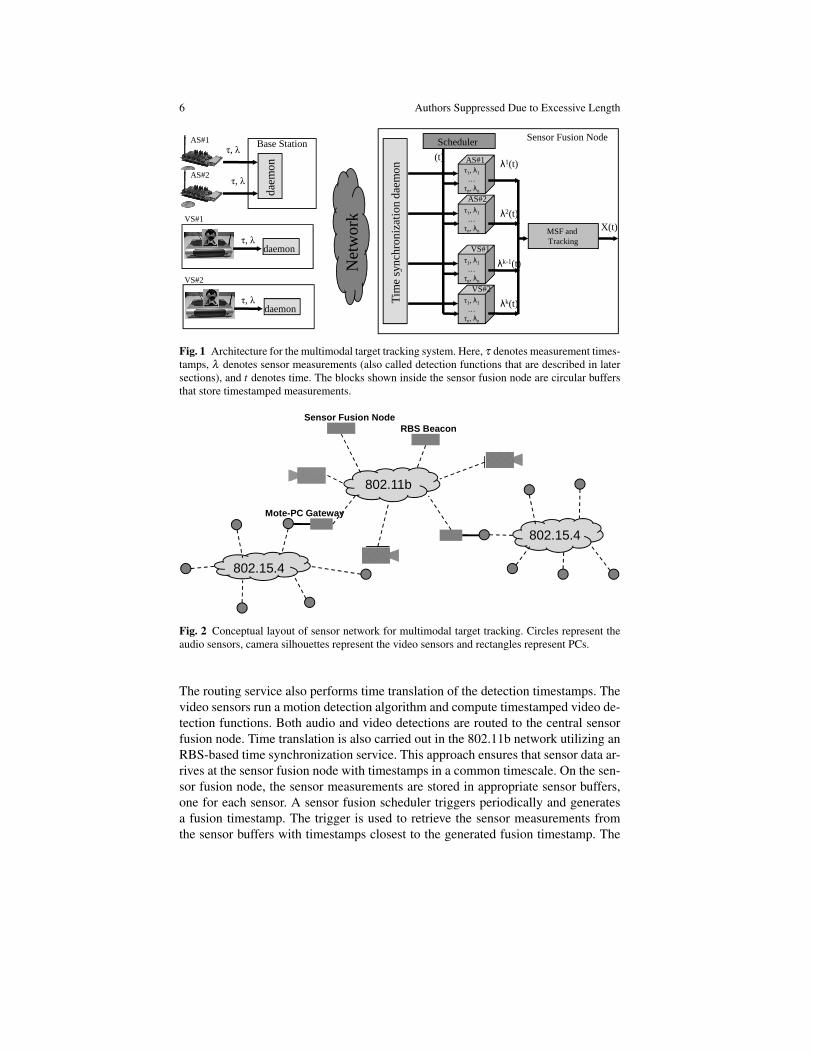
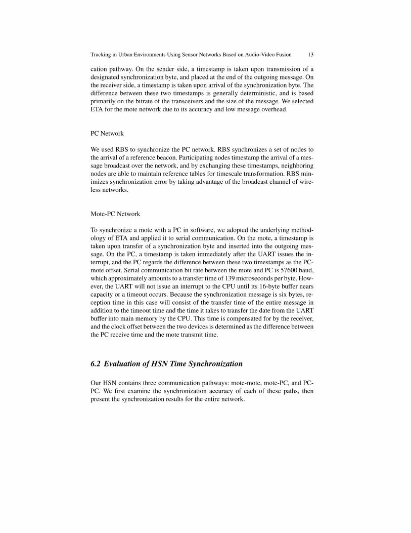
Figure 1 shows the system architecture. The audio sensors, consisting of MICAzmotes with acoustic sensor boards equipped with a microphone array, form an IEEE802.15.4 network. This network does not need to be connected; it can consist ofmultiple connected components as long as each of these component have a dedicatedmote-PC gateway. The video sensors are based on Logitech QuickCam Pro 4000cameras attached to OpenBrick-E Linux embedded PCs. These video sensors, alongwith the mote-PC gateways, the sensor fusion node and the reference broadcasterfor time synchronization (see Section 6) are all PCs forming a peer-to-peer 802.11bwireless network. Figure 2 shows the conceptual layout of the sensor network.

The audio sensors perform beamforming, and transmit the audio detections to thecorresponding mote-PC gateway utilizing a multi-hop message routing service [2].


τ1, λ1

…τn, λn

τ1, λ1

…τn, λn

τ1, λ1

…τn, λn

τ1, λ1

…τn, λn

Scheduler

MSF and Tracking

(t)λ1(t)

λ2(t)

λk-1(t)

λk(t)

X(t)

Tim

e sy

nch

ron

izat

ion

dae

mo

n

τ, λdaemon

τ, λ

τ, λ

Net

wo

rk

dae

mo

n

Base StationSensor Fusion NodeAS#1

AS#2

VS#1

VS#2

AS#1

AS#2

VS#1

VS#2

τ, λdaemon

Fig. 1 Architecture for the multimodal target tracking system. Here, τ denotes measurement times-tamps, λ denotes sensor measurements (also called detection functions that are described in latersections), and t denotes time. The blocks shown inside the sensor fusion node are circular buffersthat store timestamped measurements.

802.11b

802.15.4

802.15.4

Sensor Fusion Node

Mote-PC Gateway

RBS Beacon

802.15.4

Fig. 2 Conceptual layout of sensor network for multimodal target tracking. Circles represent theaudio sensors, camera silhouettes represent the video sensors and rectangles represent PCs.

The routing service also performs time translation of the detection timestamps. Thevideo sensors run a motion detection algorithm and compute timestamped video de-tection functions. Both audio and video detections are routed to the central sensorfusion node. Time translation is also carried out in the 802.11b network utilizing anRBS-based time synchronization service. This approach ensures that sensor data ar-rives at the sensor fusion node with timestamps in a common timescale. On the sen-sor fusion node, the sensor measurements are stored in appropriate sensor buffers,one for each sensor. A sensor fusion scheduler triggers periodically and generatesa fusion timestamp. The trigger is used to retrieve the sensor measurements fromthe sensor buffers with timestamps closest to the generated fusion timestamp. The


retrieved sensor measurements are then used for multimodal fusion and target track-ing. In this study, we developed and compared target tracking algorithms based onboth Sequential Bayesian Estimation (SBE) and MCMCDA. Note that the triggeringmechanism of the scheduler decouples the target tracking rate from the audio andvideo sensing rates, which allows us to control the rate of the tracking applicationindependently of the sensing rate.

4 Audio Beamforming

Beamforming is a signal processing algorithm for DOA estimation of a signalsource. In a typical beamforming array, each of the spatially separated microphonesreceive a time-delayed source signal. The amount of time delay at each microphonein the array depends on the microphone arrangement and the location of the source.A typical delay-and-sum single source beamformer discretizes the sensing regioninto directions, or beams, and computes a beam energy for each of them. The beamenergies are collectively called the beamform. The beam with maximum energy in-dicates the direction of the acoustic source.

Beamforming Algorithm

The data-flow diagram of our beamformer is shown in Fig. 3. The amplified micro-phone signal is sampled at a high frequency (100 KHz) to provide high resolutionfor the time delay, which is required for the closely placed microphones. The rawsignals are filtered to remove unwanted noise components. The signal is then fed toa tapped delay line (TDL), which has M different outputs to provide the requireddelays for each of the M beams. The delays are set by taking into consideration theexact relative positions of the microphones so that the resulting beams are steeredto the beam angles, θi = i 360

M degrees, for i = 0,1, ...M−1. The signal is downsam-

Fig. 3 Data-flow diagram of the real-time beamforming sensor.


pled and the M beams are formed by adding the four delayed signals together. Datablocks are formed from the data streams (with a typical block length of 5-20ms) andan FFT is computed for each block. The block power values, µ(θi), are smoothedby exponential averaging into the beam energy, λ (θi)

λt(θi) = αλ

t−1(θi)+(1−α)µ(θi) (1)

where α is an averaging factor.

Audio Hardware

In our application, the audio sensor is a MICAz mote with an onboard XilinxXC3S1000 FPGA chip that is used to implement the beamformer [40]. The onboardFlash (4MB) and PSRAM (8MB) modules allow storing raw samples of severalacoustic events. The board supports four independent analog channels, featuring anelectret microphone each, sampled at up to 1 MS/s (million samples per second). Asmall beamforming array of four microphones arranged in a 10cm×6cm rectangleis placed on the sensor node, as shown in Fig. 4(a). Since the distances betweenthe microphones are small compared to the possible distances of sources, the sen-sors perform far-field beamforming. The sources are assumed to be on the sametwo-dimensional plane as the microphone array, thus it is sufficient to perform pla-nar beamforming by dissecting the angular space into M equal angles, providing aresolution of 360/M degrees. In the experiments, the sensor boards are configuredto perform simple delay-and-sum-type beamforming in real time with M = 36, andan angular resolution of 10 degrees. Finer resolution increases the communicationrequirements.

Sensor Node

10 cm

6 cm

Fig. 4 (a) Sensor Node Showing the Microphones, (b) Beamform of acoustic source at a distanceof 50 feet and an angle of 120 degrees.


Evaluation

We test the beamformer node outdoors using recorded speech as the acoustic source.Measurements are taken by placing the source at distances of 3, 5, 10, 25, 50, 75,100, and 150 feet from the sensor, and at an angle from -180◦ to +180◦ in 5◦ incre-ments. Figure 4(b) shows the beamforming result for a single audio sensor when thesource was at a distance of 50 feet. Mean DOA measurement error for 1800 humanspeech experiments is shown in Figure 5. The smallest error was recorded when thesource was at a distance of 25 feet from the sensor. The error increases as the sourcemoves closer to the sensor. This is because the beamforming algorithm assumes aplanar wavefront, which holds for far-field sources but breaks down when the sourceis close to the sensor. However, as the distance between the source and sensor grows,error begins accumulating again as the signal-to-noise ratio decreases.

0 10 20 30 40 50 60 70 800

5

10

15

20

25

30

35

40

45

50

Range (feet)

Ang

le (

degr

ees)

Fig. 5 Human speech DOA error for distances of 3, 5, 10, 25, 50, 75 feet between acoustic sourceand beamformer node.

Messages containing the audio detection functions require 83 bytes, and includenode ID, sequence number, timestamps, and 72 bytes for 36 beam energies. Thesedata are transmitted through the network in a single message. The default TinyOSmessage size of 36 bytes was changed to 96 bytes to accommodate the entire audiomessage. The current implementation uses less than half of the total resources (logiccells, RAM blocks) of the selected mid-range FPGA device. The application runs at20 MHz, which is relatively slow in this domain—the inherent parallel processingtopology allows this slow speed. Nonetheless, the FPGA approach has a significantimpact on the power budget, the sensor draws 130mA current (at 3.3 V) which isnearly a magnitude higher then typical wireless sensor node power currents. Flash-based FPGAs and smart duty cycling techniques are promising new directions inour research project for reducing the power requirements.


5 Video Tracking

Video tracking systems seek to automatically detect moving targets and track theirmovement in a complex environment. Due to the inherent richness of the visualmedium, video based tracking typically requires a pre-processing step that focusesattention of the system on regions of interest in order to reduce the complexity ofdata processing. This step is similar to the visual attention mechanism in human ob-servers. Since the region of interest is primarily characterized by regions containingmoving targets (in the context of target tracking), robust motion detection is the firststep in video tracking. A simple approach to motion detection from video data isvia frame differencing. It compares each incoming frame with a background modeland classifies the pixels of significant variation into the foreground. The foregroundpixels are then processed for identification and tracking. The success of frame differ-encing depends on the robust extraction and maintenance of the background model.Performance of such techniques tends to degrade when there is significant cameramotion, or when the scene has significant amount of change.

Algorithm

The dataflow in Figure 6 shows the motion detection algorithm and its componentsused in our tracking application. The first component is background-foreground seg-

Bt

Gaussian bg/fgsegmentation

Median FilterDetection Function

It FtPost-

processing Filters

Dt

Fig. 6 Data-flow diagram of real-time motion detection algorithm

mentation of the currently captured frame (It ) from the camera. We use the algorithmdescribed in [19]. This algorithm uses an adaptive background mixture model forreal-time background and foreground estimation. The mixture method models eachbackground pixel as a mixture of K Gaussian distributions. The algorithm providesmultiple tunable parameters for desired performance. In order to reduce specklenoise and smooth the estimated foreground (Ft ), the foreground is passed through amedian filter. In our experiments, we use a median filter of size 3×3.

Since our sensor fusion algorithm (Section 7) utilizes only the angle of movingtargets, it is desirable and sufficient to represent the foreground in a simpler detec-tion function. Similar to the beam angle concept in audio beamforming (Section 4),the field-of-view of the camera is divided into M equally-spaced angles

θi = θmin +(i−1)θmax−θmin

M: i = 1,2, ...,M (2)


where θmin and θmax are the minimum and maximum field-of-view angles for thecamera. The detection function value for each angle is simply the number of fore-ground pixels in that direction. Formally, the detection function for the video sensorscan be defined as

λ (θi) =W

∑j∈θi

H

∑k=1

F( j,k) : i = 1,2, ...,M (3)

where F is the binary foreground image, H and W are the vertical and horizontalresolutions in pixels, respectively and j ∈ θi indicates columns in the frame that fallwithin angle θi. Figure 7 shows a snapshot of motion detection.

H

W

Fig. 7 Video detection. The frame on the left shows the input image, the frame in the middle showsthe foreground and the frame on the right shows the video detection function.

Video Post-processing

In our experiments, we gathered video data of vehicles from multiple sensors froman urban street setting. The data contained a number of real-life artifacts such asvacillating backgrounds, shadows, sunlight reflections and glint. The algorithm de-scribed above is not able to filter out such artifacts from the detections. We im-plemented two post-processing filters to improve the detection performance. Thefirst filter removes any undesirable persistent background. For this purpose we keepa background of moving averages which was removed from each detection. Thebackground update and filter equations are

bt(θ) = αbt−1(θ)+(1−α)λ t(θ) (4)λ

t(θ) = λt(θ)−bt−1(θ) (5)

where bt(θ) is the moving average background, and λ t(θ) is the detection functionat time t. The second filter removes any sharp spikes (typically caused by sunlightreflections and glint). For this we convolved the detection function with a smalllinear kernel to add a blurring effect. This essentially reduces the effect of any sharpspikes in detection function due to glints. The equation for this filter is

λt(θ) = λ

t(θ)∗ k (6)


where k is a 7×1 vector of equal weights, and ∗ denotes convolution.We implemented the motion detection algorithm using OpenCV (open source

computer vision) library. We use Linux PCs equipped with the QuickCam Pro 4000as video sensors. The OpenBrick-E has 533 MHz CPU, 128 MB RAM, and a802.11b wireless adapter. The QuickCam Pro supports up to 640× 480 pixel res-olution and up to 30 frames-per-second frame rate. Our motion detection algorithmimplementation runs at 4 frames-per-second and 320× 240 pixel resolution. Thenumber of angles in Equation (2) is M = 160.

6 Time Synchronization

In order to seamlessly fuse time-dependent audio and video sensor data for trackingmoving objects, participating nodes must have a common notion of time. Althoughseveral microsecond-accurate synchronization protocols have emerged for wirelesssensor networks (e.g. [12, 14, 27, 35]), achieving accurate synchronization in a het-erogeneous sensor network is not a trivial task.

6.1 Synchronization Methodology

Attempting to synchronize the entire network using a single protocol will intro-duce a large amount of error. For example, TPSN [14], FTSP [27], and RITS [35]were all designed to run on the Berkeley Motes, and assume the operating sys-tem is tightly integrated with the radio stack. Attempting to use such protocols onan 802.11 PC network will result in poor synchronization accuracy because thenecessary low-level hardware control is difficult to achieve. Reference BroadcastSynchronization (RBS) [12], although flexible when it comes to operating systemand computing platform, is accurate only when all nodes have access to a commonnetwork medium. A combined network of motes and PCs will be difficult to syn-chronize using RBS because each platform uses different communication protocolsand wireless frequencies. Instead, we adopted a hybrid approach [2], which pairs aspecific network with the synchronization protocol that provides the most accuracywith the least amount of overhead. To synchronize the entire network, it is neces-sary for gateway nodes (i.e., nodes connecting multiple networks,) to handle severalsynchronization mechanisms.

Mote Network

We used Elapsed Time on Arrival (ETA) [23] to synchronize the mote network.ETA timestamps synchronization messages at transmit and receive time, thus re-moving the largest amount of nondeterministic message delay from the communi-


cation pathway. On the sender side, a timestamp is taken upon transmission of adesignated synchronization byte, and placed at the end of the outgoing message. Onthe receiver side, a timestamp is taken upon arrival of the synchronization byte. Thedifference between these two timestamps is generally deterministic, and is basedprimarily on the bitrate of the transceivers and the size of the message. We selectedETA for the mote network due to its accuracy and low message overhead.

PC Network

We used RBS to synchronize the PC network. RBS synchronizes a set of nodes tothe arrival of a reference beacon. Participating nodes timestamp the arrival of a mes-sage broadcast over the network, and by exchanging these timestamps, neighboringnodes are able to maintain reference tables for timescale transformation. RBS min-imizes synchronization error by taking advantage of the broadcast channel of wire-less networks.

Mote-PC Network

To synchronize a mote with a PC in software, we adopted the underlying method-ology of ETA and applied it to serial communication. On the mote, a timestamp istaken upon transfer of a synchronization byte and inserted into the outgoing mes-sage. On the PC, a timestamp is taken immediately after the UART issues the in-terrupt, and the PC regards the difference between these two timestamps as the PC-mote offset. Serial communication bit rate between the mote and PC is 57600 baud,which approximately amounts to a transfer time of 139 microseconds per byte. How-ever, the UART will not issue an interrupt to the CPU until its 16-byte buffer nearscapacity or a timeout occurs. Because the synchronization message is six bytes, re-ception time in this case will consist of the transfer time of the entire message inaddition to the timeout time and the time it takes to transfer the date from the UARTbuffer into main memory by the CPU. This time is compensated for by the receiver,and the clock offset between the two devices is determined as the difference betweenthe PC receive time and the mote transmit time.

6.2 Evaluation of HSN Time Synchronization

Our HSN contains three communication pathways: mote-mote, mote-PC, and PC-PC. We first examine the synchronization accuracy of each of these paths, thenpresent the synchronization results for the entire network.


Mote Network

We evaluated synchronization accuracy in the mote network with the pairwise dif-ference method. Two nodes simultaneously timestamp the arrival of an event bea-con, then forward the timestamps to a sink node two hops away. At each hop, thetimestamps are converted to the local timescale. The synchronization error is thedifference between the timestamps at the sink node. For 100 synchronizations, theaverage error is 5.04µs, with a maximum of 9µs.

PC Network

We used a separate RBS transmitter to broadcast a reference beacon every ten sec-onds over 100 iterations. Synchronization error, determined using the pairwise dif-ference method, was as low as 17.51µs on average, and 2050.16µs maximum. Theworst-case error is significantly higher than reported in [12] because the OpenBrick-E wireless network interface controllers in our experimental setup are connected viaUSB, which has a default polling frequency of 1 kHz. For our tracking application,this is acceptable because we use a sampling rate of 4 Hz. Note that the reason forselecting such a low sampling rate is due to bandwidth constraints and interferenceand not because of synchronization error.

Mote-PC Connection

GPIO pins on the mote and PC were connected to an oscilloscope, and set highupon timestamping. The resulting output signals were captured and measured. Thetest was performed over 100 synchronizations, and the resulting error was 7.32µson average, and did not exceed 10µs. The majority of the error is due to jitter, bothin the UART and the CPU. A technique to compensate for such jitter on the motesis presented in [27], however, we did not attempt it on the PCs.

HSN

We evaluated synchronization accuracy across the entire network using the pair-wise difference method. Two motes timestamped the arrival of an event beacon,and forwarded the timestamp to the network sink, via one mote and two PCs. RBSbeacons were broadcast at four-second intervals, and therefore clock skew compen-sation was unnecessary, because synchronization error due to clock skew would beinsignificant compared with offset error. The average error over the 3-hop networkwas 101.52µs, with a maximum of 1709µs. The majority of this error is due to thepolling delay from the USB wireless network controller. However, synchronizationaccuracy is still sufficient for audio and video sensor fusion at 4Hz.


6.3 Synchronization Service

The implementation used in these experiments was bundled into a time synchro-nization and routing service for sensor fusion applications. Figure 8 illustrates theinteraction of each component within the service. The service interacts with sensingapplications that run on the local PC, as well as other service instances running onremote PCs. The service accepts timestamped event messages on a specific port,converts the embedded timestamp to the local timescale, and forwards the messagetoward the sensor-fusion node. The service uses reference broadcasts to maintainsynchronization with the rest of the PC network. In addition, the service acceptsmote-based event messages, and converts the embedded timestamps using the ETA-based serial timestamp synchronization method outlined above. Kernel modifica-tions in the serial and wireless drivers were required in order to take accurate times-tamps. Upon receipt of a designated synchronization byte, the time is recorded andpassed up to the synchronization service in the user space. The modifications areunobtrusive to other applications using the drivers, and the modules are easy to loadinto the kernel. The mote implementation uses the TimeStamping interface, pro-vided with the TinyOS distribution [25]. A modification was made to the UARTinterface to insert a transmission timestamp into the event message as it is beingtransmitted between the mote and PC. The timestamp is taken immediately beforea synchronization byte is transmitted, then inserted at the end of the message.

Fig. 8 PC-based time synchronization service.


7 Multimodal Target Tracking

This section describes the tracking algorithm and the approach for fusing the audioand video data based on sequential Bayesian estimation. We use following notation:Superscript t denotes discrete time (t ∈ Z+), subscript k ∈ {1, ...,K} denotes thesensor index, where K is the total number of sensors in the network, the target stateat time t is denoted as x(t), and the sensor data at time t is denoted as z(t).

7.1 Sequential Bayesian Estimation

We use sequential Bayesian estimation to estimate the target state x(t) at time t,similar to the approach presented in [26]. In sequential Bayesian estimation, the tar-get state is estimated by computing the posterior probability density p(x(t+1)|z(t+1))using a Bayesian filter described by

p(x(t+1)|z(t+1)) ∝ p(z(t+1)|x(t+1))∫

p(x(t+1)|x(t))p(x(t)|z(t))dx(t) (7)

where p(x(t)|z(t)) is the prior density from the previous step, p(z(t+1)|x(t+1)) is thelikelihood given the target state, and p(x(t+1)|x(t)) is the prediction for the targetstate x(t+1) given the current state x(t) according to a target motion model. Sincewe are tracking moving vehicles it is reasonable to use a directional motion modelbased on the target velocity. The directional motion model is described by

x(t+1) = x(t) + v+U [−δ ,+δ ] (8)

where x(t) is the target state time t, x(t+1) is the predicted state, v is the target velocity,and U [−δ ,+δ ] is a uniform random variable.

Because the sensor models (described later in Subsection 7.2) are nonlinear, theprobability densities cannot be represented in a closed form. It is, therefore, reason-able to use a nonparametric representation for the probability densities. The non-parametric densities are represented as discrete grids in 2D space, similar to [26].For nonparametric representation, the integration term in Equation (7) becomes aconvolution operation between the motion kernel and the prior distribution. Theresolution of the grid representation is a trade-off between tracking resolution andcomputational capacity.

Centralized Bayesian Estimation

Since we use resource constrained mote class sensors, centralized Bayesian esti-mation is a reasonable approach because of its modest computational requirements.The likelihood function in Equation (7) can be calculated either as a product or


weighted summation of the individual likelihood functions. We describe the twomethods next.

Product of Likelihood functions

Let pk(z(t)|x(t)) denote the likelihood function from sensor k. If the sensor observa-tions are mutually independent conditioned on the target state, the likelihood func-tions from multiple sensors are combined as

p(z(t)|x(t)) = ∏k=1,...,K

pk(z(t)|x(t)) (9)

Weighted-Sum of Likelihood functions

An alternative approach to combine the likelihood functions is to compute theirweighted-sum. This approach allows us to give different weights to different sen-sor data. These weights can be used to incorporate sensor reliability and quality ofsensor data. We define a quality index q(t)

k for each sensor k as

q(t)k = rk max

θ

(λ (t)k (θ))

where rk is a measure of sensor reliability and λ(t)k (θ) is the sensor detection func-

tion. The combined likelihood function is given by

p(z(t)|x(t)) =∑k=1,...,K q(t)

k pk(z(t)|x(t))

∑k=1,...,K q(t)k

(10)

We experimented with both methods in our evaluation. The product method pro-duces more accurate results with low uncertainty in target state. The weighted-summethod performs better in cases with high sensor conflict, though it suffers fromhigh uncertainty. The results are presented in Section 8.

Hybrid Bayesian Estimation

In sensor fusion a big challenge is to account for conflicting sensor data. Whensensor conflict is very high, sensor fusion algorithms produce false or meaninglessfusion results [18]. Reasons for sensor conflict are sensor locality, different sensormodalities, and sensor faults. Selecting and clustering the sensors in different groupsbased on locality or modality can mitigate poor performance due to sensor conflict.For example, clustering the sensors close to the target and fusing the data from onlythe sensors in the cluster would remove the conflict caused by distant sensors.


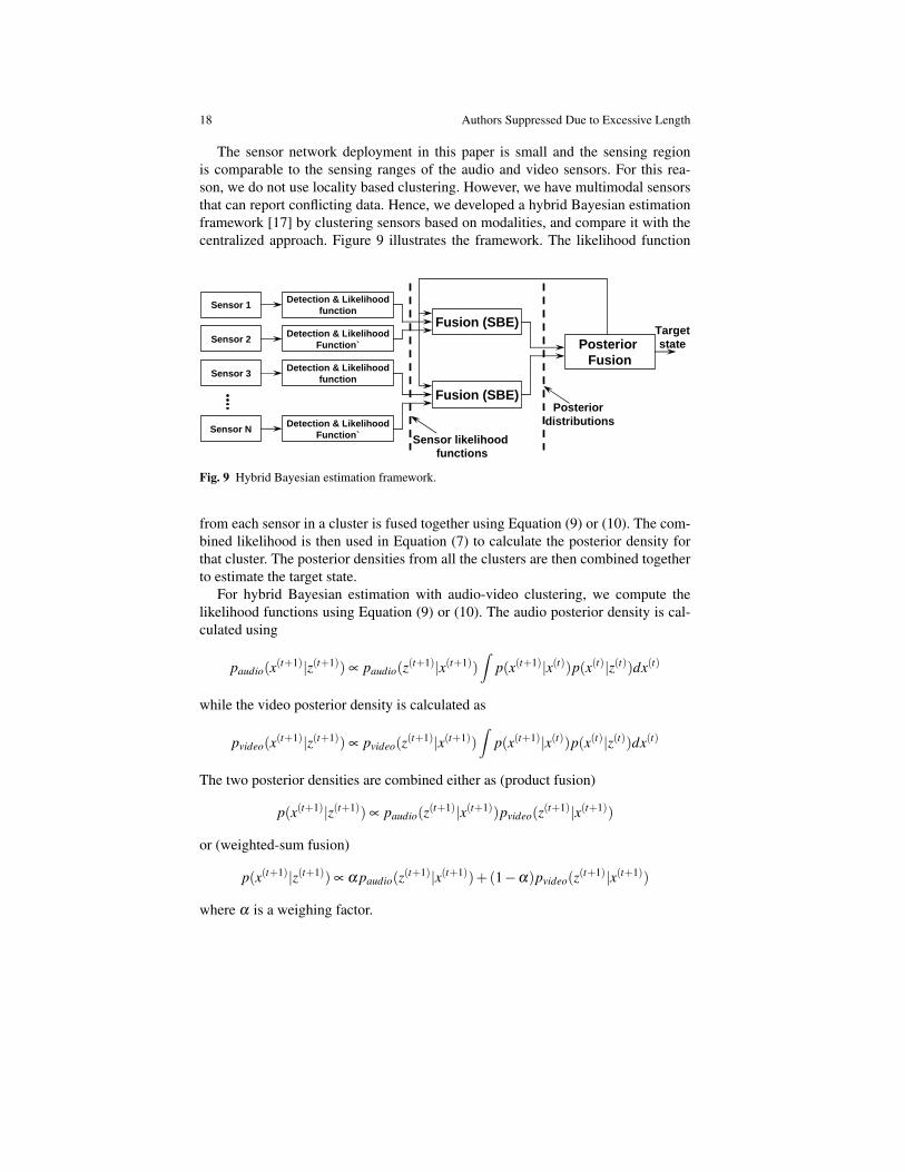
The sensor network deployment in this paper is small and the sensing regionis comparable to the sensing ranges of the audio and video sensors. For this rea-son, we do not use locality based clustering. However, we have multimodal sensorsthat can report conflicting data. Hence, we developed a hybrid Bayesian estimationframework [17] by clustering sensors based on modalities, and compare it with thecentralized approach. Figure 9 illustrates the framework. The likelihood function

Sensor 1

Sensor 2

Sensor 3

Sensor N

Detection & Likelihoodfunction

Fusion (SBE)

Fusion (SBE)

Posterior Fusion

Detection & LikelihoodFunction`

Detection & Likelihoodfunction

Detection & LikelihoodFunction` Sensor likelihood

functions

Posterior distributions

Target state

Fig. 9 Hybrid Bayesian estimation framework.

from each sensor in a cluster is fused together using Equation (9) or (10). The com-bined likelihood is then used in Equation (7) to calculate the posterior density forthat cluster. The posterior densities from all the clusters are then combined togetherto estimate the target state.

For hybrid Bayesian estimation with audio-video clustering, we compute thelikelihood functions using Equation (9) or (10). The audio posterior density is cal-culated using

paudio(x(t+1)|z(t+1)) ∝ paudio(z(t+1)|x(t+1))∫

p(x(t+1)|x(t))p(x(t)|z(t))dx(t)

while the video posterior density is calculated as

pvideo(x(t+1)|z(t+1)) ∝ pvideo(z(t+1)|x(t+1))∫

p(x(t+1)|x(t))p(x(t)|z(t))dx(t)

The two posterior densities are combined either as (product fusion)

p(x(t+1)|z(t+1)) ∝ paudio(z(t+1)|x(t+1))pvideo(z(t+1)|x(t+1))

or (weighted-sum fusion)

p(x(t+1)|z(t+1)) ∝ α paudio(z(t+1)|x(t+1))+(1−α)pvideo(z(t+1)|x(t+1))

where α is a weighing factor.


7.2 Sensor Models

We use a nonparametric model for the audio sensors, while a parametric mixture-of-Gaussian model for the video sensors is used to mitigate the effect of sensor conflictin object detection.

Audio Sensor Model

The nonparametric DOA sensor model for a single audio sensor is the piecewiselinear interpolation of the audio detection function

λ (θ) = wλ (θi−1)+(1−w)λ (θi), if θ ∈ [θi−1,θi]

where w = (θi−θ)/(θi−θi−1).

Video Sensor Model

The video detection algorithm captures the angle of one or more moving objects.The detection function from Equation (3) can be parametrized as a mixture-of-Gaussian

λ (θ) =n

∑i=1

ai fi(θ)

where n is the number of components, fi(θ) is the probability density, and ai is themixing proportion for component i. Each component is a Gaussian density given byfi(θ) = N (θ |µi,σ

2i ), where the component parameters µi, σ2

i and ai are calculatedfrom the detection function.

Likelihood Function

The 2D search space is divided into N rectangular cells with center points at (xi,yi),for i = 1,2, ...,N as illustrated in Figure 10. The likelihood function value for kth

sensor at ith cell is the average value of the detection function in that cell, given by

pk(z|x) = pk(xi,yi) =1

(ϕ(k,i)B −ϕ

(k,i)A )

∑ϕ

(k,i)A ≤θ≤ϕ

(k,i)B

λk(θ)


0

0.2

0.4

0.6

0.8

1

P0(xi,yi)P1P2

P4P3

Qk (xk,yk)Rk

φA

φB

φ0

Fig. 10 Computation of the likelihood value for kth sensor at ith cell, (xi,yi). The cell is centeredat P0 with vertices at P1, P2, P3, and P4. The angular interval subtended at the sensor due to the ith

cell is θ ∈ [ϕ(k,i)A ,ϕ

(k,i)B ], or θ ∈ [0,2π] if the sensor is inside the cell.

7.3 Multiple-Target Tracking

The essence of the multi-target tracking problem is to find a track of each objectfrom noisy measurements. If the sequence of measurements associated with eachobject is known, multi-target tracking reduces to a set of state estimation problemsfor which many efficient algorithms are available. Unfortunately, the associationbetween measurements and objects is unknown. The data association problem is towork out which measurements were generated by which objects; more precisely, werequire a partition of measurements such that each element of a partition is a collec-tion of measurements generated by a single object or noise. Due to this data asso-ciation problem, the complexity of the posterior distribution of the states of objectsgrows exponentially as time progresses. It is well-known that the data associationproblem is NP-hard [32], so we do not expect to find efficient, exact algorithms forsolving this problem.

In order to handle highly nonlinear and non-Gaussian dynamics and observa-tions, a number of methods based on particle filters has recently been developed totrack multiple objects in video [30, 20]. Although particle filters are highly effec-tive in single-target tracking, it is reported that they provide poor performance inmulti-target tracking [20]. This is because a fixed number of particles is insufficientto represent the posterior distribution with the exponentially increasing complexity(due to the data association problem). As shown in [20, 43], an efficient alternative isto use Markov chain Monte Carlo (MCMC) to handle the data association problemin multi-target tracking.

For our problem, there is an additional complexity. We do not assume the num-ber of objects is known. A single-scan approach, which updates the posterior basedonly on the current scan of measurements, can be used to track an unknown number


of targets with the help of trans-dimensional MCMC [43, 20] or a detection algo-rithm [30]. But a single-scan approach cannot maintain tracks over long periodsbecause it cannot revisit previous, possibly incorrect, association decisions in thelight of new evidence. This issue can be addressed by using a multi-scan approach,which updates the posterior based on both current and past scans of measurements.The well-known multiple hypothesis tracking (MHT) [33] is a multi-scan tracker,however, it is not widely used due to its high computational complexity.

A newly developed algorithm, called Markov chain Monte Carlo data associa-tion (MCMCDA), provides a computationally desirable alternative to MHT [29].The simulation study in [29] showed that MCMCDA was computationally efficientcompared to MHT with heuristics (i.e., pruning, gating, clustering, N-scan-backlogic and k-best hypotheses). In this chapter, we use the online version of MCM-CDA to track multiple objects in a 2-D plane. Due to the page limitation, we omitthe description of the algorithm in this paper and refer interested readers to [29].

8 Evaluation

In this section, we evaluate target tracking algorithms based on the sequentialBayesian estimation and MCMCDA.

8.1 Sequential Bayesian Estimation

Video node 3

Video node 1

Video node 2

1 2 3

4 5 6

Audio SensorsVideo Sensors

Sensor Fusion Center

36.5 ft

15 ft

92 ft

76 ft

Fig. 11 Experimental setup

The deployment of our multimodal target tracking system is shown in Figure11. We employ 6 audio sensors and 3 video sensors deployed on either side of aroad. The complex urban street environment presents many challenges includinggradual change of illumination, sunlight reflections from windows, glints due tocars, high visual clutter due to swaying trees, high background acoustic noise due


to construction and acoustic multipath effects due to tall buildings. The objective ofthe system is to detect and track vehicles using both audio and video under theseconditions.

Sensor localization and calibration for both audio and video sensors are required.In our experimental setup, the sensor nodes are manually placed at marked locationsand orientations. The audio sensors are placed on 1 meter high tripods to minimizeaudio clutter near the ground. An accurate self-calibration technique, e.g. [16, 28], isdesirable for a target tracking system. Our experimental setup consists of two wire-less networks as described in Section 3. The mote network is operating on channel26 (2.480 GHz) while the 802.11b network is operating on channel 6 (2.437 GHz).Both the channels are non-overlapping and different from the infrastructure wire-less network, which operates on channel 11 (2.462 GHz). We choose these non-overlapping channels to minimize interference and are able to achieve less than 2%packet loss.

We gather audio and video detection data for a total duration of 43 minutes. Ta-ble 1 presents the parameter values that we use in our tracking system. We run our

Number of beams in audio beamforming, Maudio 36Number of angles in video detection Mvideo 160Sensing region (meters) 35×20Cell size (meters) 0.5×0.5

Table 1 Parameters used in experimental setup

sensor fusion and tracking system online using centralized sequential Bayesian es-timation based on the product of likelihood functions. We also collect all the audioand video detection data for offline evaluation. This way we are able to experimentwith different fusion approaches on the same data set. For offline evaluations, weshortlist 10 vehicle tracks where there is only a single target in the sensing region.The average duration of tracks is 4.25 sec with 3.0 sec minimum and 5.5 sec maxi-mum. The tracked vehicles are part of an uncontrolled experiment. The vehicles aretraveling on road at a speed of 20-30 mph speed.

Sequential Bayesian estimation requires a prior density of the target state. Weinitialize the prior density using a simple detection algorithm based on audio data.If the maximum of the audio detection functions exceeds a threshold, we initializethe prior density based on the audio detection.

In our simulations, we experiment with eight different approaches. We use audio-only, video-only and audio-video sensor data for sensor fusion. For each of thesedata sets, the likelihood is computed either as the weighted-sum or product of thelikelihood function for the individual sensors. For the audio-video data, we usecentralized and hybrid fusion. Following is the list of different target tracking ap-proaches.

1. audio-only, weighted-sum (AS)2. video-only, weighted-sum (VS)


3. audio-video, centralized, weighted-sum (AVCS)4. audio-video, hybrid, weighted-sum (AVHS)5. audio-only, likelihood product (AP)6. video-only, likelihood product (VP)7. audio-video, centralized, likelihood product (AVCP)8. audio-video, hybrid, likelihood product (AVHP)

The ground truth is estimated post-facto based on the video recording by a sep-arate camera. The standalone ground truth camera is not part of any network, andhave the sole responsibility of recording ground truth video. For evaluation of track-ing accuracy, the center of mass of the vehicle is considered to be the true location.

Figure 12 shows the tracking error for a representative vehicle track. The tracking

Fig. 12 Tracking error (a) weighted sum, (b) product

error when audio data is used is consistently lower than the case when the video datais used. When we use both audio and video data, the tracking error is lower thaneither of those considered alone. Figure 13 shows the determinant of the covarianceof the target state for the same vehicle track. The covariance, which is an indicator of

Fig. 13 Tracking variance (a) weighted sum, (b) product

uncertainty in the target state is significantly lower for product fusion than weighted-sum fusion. In general, covariance for audio-only tracking is higher than video-onlytracking, while using both modalities lowers the uncertainty.

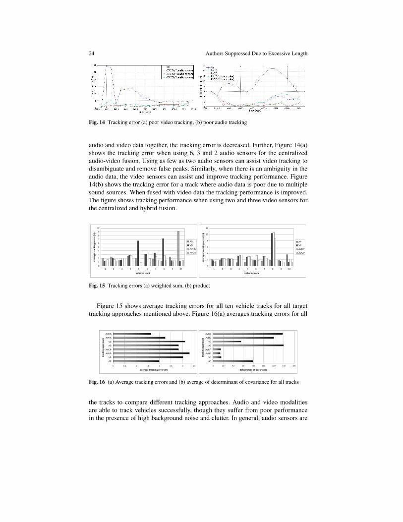
Figure 14(a) shows the tracking error in the case of fusion based on weighted-sum. The tracking error when using only video data shows a large value at timet = 1067 second. In this case, the video data has false peaks not corresponding tothe target. The audio fusion works fine for this track. As expected, when we use both


Fig. 14 Tracking error (a) poor video tracking, (b) poor audio tracking

audio and video data together, the tracking error is decreased. Further, Figure 14(a)shows the tracking error when using 6, 3 and 2 audio sensors for the centralizedaudio-video fusion. Using as few as two audio sensors can assist video tracking todisambiguate and remove false peaks. Similarly, when there is an ambiguity in theaudio data, the video sensors can assist and improve tracking performance. Figure14(b) shows the tracking error for a track where audio data is poor due to multiplesound sources. When fused with video data the tracking performance is improved.The figure shows tracking performance when using two and three video sensors forthe centralized and hybrid fusion.

0

1

2

3

4

5

6

7

8

9

10

1 2 3 4 5 6 7 8 9 10

vehicle track

aver

age

trac

kin

g e

rro

r (m

)

AS

VS

AVHS

AVCS

0

2

4

6

8

10

12

1 2 3 4 5 6 7 8 9 10

vehicle track

aver

age

trac

kin

g e

rro

r (m

)

AP

VP

AVHP

AVCP

Fig. 15 Tracking errors (a) weighted sum, (b) product

Figure 15 shows average tracking errors for all ten vehicle tracks for all targettracking approaches mentioned above. Figure 16(a) averages tracking errors for all

0 0.5 1 1.5 2 2.5 3 3.5

AP

VP

AVHP

AVCP

AS

VS

AVHS

AVCS

trac

kin

g a

pp

roac

h

average tracking error (m)

0 20 40 60 80 100 120 140 160

AP

VP

AVHP

AVCP

AS

VS

AVHS

AVCS

trac

kin

g a

pp

roac

h

determinant of covariance

Fig. 16 (a) Average tracking errors and (b) average of determinant of covariance for all tracks

the tracks to compare different tracking approaches. Audio and video modalitiesare able to track vehicles successfully, though they suffer from poor performancein the presence of high background noise and clutter. In general, audio sensors are


able to track vehicles with good accuracy, but they suffer from high uncertainty andpoor sensing range. Video tracking is not very robust in the presence of multipletargets and noise. As expected, fusing the two modalities consistently gives betterperformance. There are some cases where audio tracking performance is better thanfusion. This is due to poor performance of video tracking.

Fusion based on the product of likelihood functions gives better performancebut it is more vulnerable to sensor conflict and errors in sensor calibration. Theweighted-sum approach is more robust to conflicts and sensor errors, but it suffersfrom high uncertainty. The centralized estimation framework consistently performsbetter than the hybrid framework.

Figure 17 shows the determinant of the covariance for all tracks and all ap-proaches. Figure 16(b) presents averages of covariance measure for all tracks to

0

20

40

60

80

100

120

140

160

180

1 2 3 4 5 6 7 8 9 10

vehicle track

det

erm

inan

t o

f co

vari

ance

AS

VS

AVHS

AVCS

0

20

40

60

80

100

120

140

1 2 3 4 5 6 7 8 9 10

vehicle track

det

erm

inan

t o

f co

vari

ance

AP

VP

AVHP

AVCP

Fig. 17 Determinant of covariance (a) weighted sum, (b) product

compare the performance of tracking approaches. Among modalities, video sensorshave lower uncertainty than audio sensors. Among the fusion techniques, productfusion produces lower uncertainty, as expected. There was no definite comparisonbetween the centralized and hybrid approach, though the latter seems to producelower uncertainty in the case of weighted-sum fusion.

The average tracking error of 2 meters is reasonable considering the fact that avehicle is not a point source, and the cell size used in fusion is 0.5 meters.

8.2 MCMCDA

The audio and video data gathered for target tracking based on sequential Bayesianestimation is reused to evaluate target tracking based on MCMCDA. For MCMCDAevaluation, we experiment with six different approaches. We use audio-only (A),video-only (V) and audio-video (AV) sensor data for sensor fusion. For each ofthese data sets, the likelihood is computed either as the weighted-sum or product ofthe likelihood functions for individual sensors.


8.2.1 Single Target

We shortlist 9 vehicle tracks with a single target in the sensing region. The averageduration of tracks is 3.75 sec with 2.75 sec minimum and 4.5 sec maximum. Figure18 shows the target tracking result for two different representative vehicle tracks.The figure also shows the raw observations obtained from the multimodal sensorfusion and peak detection algorithms. Figure 19 shows average tracking errors for

Fig. 18 Target Tracking (a) no missed detection (b) with missed detections

0

1

2

3

4

5

1 2 3 4 5 6 7 8 9

vehicle track

aver

age

trac

kin

g

erro

r (m

)

audio video audio-video

0

0.5

1

1.5

2

2.5

3

3.5

1 2 3 4 5 6 7 8 9

vehicle track

aver

age

trac

king

err

or (m

)

audio

video

audio-video

Fig. 19 Tracking errors (a) weighted sum fusion, and (b) product fusion

all vehicle tracks for the weighted-sum fusion and product fusion approaches. Themissing bars indicate that the data association algorithm is not able to successfullyestimate a track for the target. Figure 20 averages tracking errors for all the tracksto compare different tracking approaches. The figure also shows the comparison ofthe performance of tracking based on sequential Bayesian estimation to MCMCDAbased tracking. The performance of MCMCDA is consistently better than sequentialBayesian estimation. Table 2 compares average tracking errors and tracking successacross likelihood fusion and sensor modality. Tracking success is defined as thepercentage of correct tracks that the algorithm is successfully able to estimate. Ta-ble 3 shows the reduction in tracking error for audio-video fusion over audio-onlyand video-only approaches. For summation fusion, the audio-video fusion is able to


video

av

audio

video

av

trac

kin

g a

pp

roac

hmcmcda

sbe

Summ

Prod

0 0.5 1 1.5 2 2.5 3 3.5

audio

video

average tracking error (m)

Prod

Fig. 20 Average tracking errors for all estimated tracks. A comparison with sequential Bayesianestimation based tracking is also shown.

Average error (m) Tracking success

Fusion Summ 1.93 74%Prod 1.58 59%

ModalityAudio 1.49 89%Video 2.44 50%AV 1.34 61%

Table 2 Average tracking error and tracking success

reduce tracking error by an average of 0.26 m and 1.04 m for audio and video ap-proaches, respectively. The audio-video fusion improves accuracy for 57% and 75%of the tracks for audio and video approaches, respectively. For the rest of the tracks,the tracking error either increased or remained same. Similar results are presentedfor product fusion in Table 3. In general, audio-video fusion improves over eitheraudio or video or both approaches. Video cameras were placed at an angle along the

Summ ProdAverageerror re-duction(m)

Tracksim-proved

Averageerror re-duction(m)

Tracksim-proved

Audio 0.26 57% 0.14 100%Video 1.04 75% 0.90 67%

Table 3 Average reduction in tracking error for AV over audio and video-only for all estimatedtracks


road to maximize coverage of the road. This makes video tracking very sensitive tocamera calibration errors and camera placement. Also, an occasional obstruction infront of a camera confused the tracking algorithm which took a while to recover. Anaccurate self-calibration technique, e.g. [16, 28], is desirable for better performanceof a target tracking system.

8.2.2 Multiple Targets

Many tracks with multiple moving vehicles in the sensing region were recordedduring the experiment. Most of them have vehicles moving in the same direction.Only a few tracks include multiple vehicles crossing each other. Figure 21 shows

Fig. 21 Multiple Target Tracking (a) XY plot (b) X-Coordinate with time

the multiple target tracking result for three vehicles where two of them are crossingeach other. Figure 21(a) shows the three tracks with the ground truth, while Figure21(b) shows the x-coordinate of the tracks with time. The average tracking errorsfor the three tracks are 1.29m, 1.60m and 2.20m. Fig. 21 shows the result when onlyvideo data from the three video sensors is used. Multiple target tracking with audiodata could not distinguish between targets when they cross each other. This is dueto the fact that beamforming is done assuming acoustic signals are generated from


a single source. Acoustic beamforming methods exist for detecting and estimatingmultiple targets [7].

9 Conclusions

We have developed a multimodal tracking system for an HSN consisting of audioand video sensors. We presented various approaches for multimodal sensor fusionand two approaches for target tracking, which are based on sequential Bayesian esti-mation and MCMCDA algorithm. We have evaluated the performance of the track-ing system using an HSN of six mote-based audio sensors and three PC webcamera-based video sensors. We evaluated and compared the performance for both thetracking approaches. Time synchronization across the HSN allows the fusion of thesensor data. We have deployed the HSN and evaluated the performance by track-ing moving vehicles in an uncontrolled urban environment. We have shown that,in general, fusion of audio and video data can improve the tracking performance.Currently, our system is not robust to multiple acoustic sources or multiple movingtargets. An accurate self-calibration technique and robust audio and video sensingalgorithms for multiple targets are required for better performance. A related chal-lenge is sensor conflict that can degrade the performance of any fusion method andneeds to be carefully considered. As in all sensor network applications, scalabilityis an important aspect that has to be considered as well.

References

1. A. M. Ali, K. Yao, T. C. Collier, C. E. Taylor, D. T. Blumstein, and L. Girod. An empiri-cal study of collaborative acoustic source localization. In IPSN ’07: Proceedings of the 6thinternational conference on Information processing in sensor networks, pages 41–50, 2007.

2. I. Amundson, B. Kusy, P. Volgyesi, X. Koutsoukos, and A. Ledeczi. Time synchronizationin heterogeneous sensor networks. In International Conference on Distributed Computing inSensor Networks (DCOSS 2008), 2008.

3. M. J. Beal, N. Jojic, and H. Attias. A graphical model for audiovisual object tracking. vol-ume 25, pages 828–836, 2003.

4. P. Bergamo, S. Asgari, H. Wang, D. Maniezzo, L. Yip, R. E. Hudson, K. Yao, and D. Estrin.Collaborative sensor networking towards real-time acoustical beamforming in free-space andlimited reverberence. In IEEE Transactions On Mobile Computing, volume 3, pages 211–224,2004.

5. S. T. Birchfield. A unifying framework for acoustic localization. In Proceedings of the 12thEuropean Signal Processing Conference (EUSIPCO), Vienna, Austria, September 2004.

6. N. Checka, K. Wilson, V. Rangarajan, and T. Darrell. A probabilistic framework for multi-modal multi-person tracking. In IEEE Workshop on Multi-Object Tracking, 2003.

7. J. C. Chen, K. Yao, and R. E. Hudson. Acoustic source localization and beamforming: theoryand practice. In EURASIP Journal on Applied Signal Processing, pages 359–370, April 2003.

8. T. Darrell, D. Demirdjian, N. Checka, and P. Felzenszwalb. Plan-view trajectory estimationwith dense stereo background models. In Proceedings. Eighth IEEE International Conferenceon Computer Vision (ICCV 2001), 2001.


9. M. Ding, A. Terzis, I.-J. Wang, and D. Lucarelli. Multi-modal calibration of surveillancesensor networks. In Military Communications Conference, MILCOM 2006, 2006.

10. E. Duarte-Melo and M. Liu. Analysis of energy consumption and lifetime of heterogeneouswireless sensor networks. In IEEE Globecom, 2002.

11. A. Elgammal, D. Harwood, and L. Davis. Non-parametric model for background subtraction.In IEEE ICCV’99 Frame-Rate workshop, 1999.

12. J. Elson, L. Girod, and D. Estrin. Fine-grained network time synchronization using referencebroadcasts. In Operating Systems Design and Implementation (OSDI), 2002.

13. N. Friedman and S. Russell. Image segmentation in video sequences: A probabilistic ap-proach. In Conference on Uncertainty in Artificial Intelligence, 1997.

14. S. Ganeriwal, R. Kumar, and M. B. Srivastava. Timing-sync protocol for sensor networks. InACM SenSys, 2003.

15. L. Girod, V. Bychkovsky, J. Elson, and D. Estrin. Locating tiny sensors in time and space: Acase study. In ICCD, 2002.

16. L. Girod, M. Lukac, V. Trifa, and D. Estrin. The design and implementation of a self-calibrating distributed acoustic sensing platform. In SenSys ’06, 2006.

17. D. Hall and J. Llinas. An introduction to multisensor data fusion. In Proceedings of the IEEE,volume 85, pages 6–23, 1997.

18. H. Y. Hau and R. L. Kashyap. On the robustness of Dempster’s rule of combination. In IEEEInternational Workshop on Tools for Artificial Intelligence, 1989.

19. P. KaewTraKulPong and R. B. Jeremy. An improved adaptive background mixture model forrealtime tracking with shadow detection. In Workshop on Advanced Video Based SurveillanceSystems (AVBS), 2001.

20. Z. Khan, T. Balch, and F. Dellaert. MCMC-based particle filtering for tracking a variable num-ber of interacting targets. IEEE Transactions on Pattern Analysis and Machine Intelligence,27(11):1805–1918, Nov. 2005.

21. D. Koller, J. Weber, T. Huang, J. Malik, G. Ogasawara, B. Rao, and S. Russell. Towards robustautomatic traffic scene analysis in realtime. In IEEE Conference on Decision and Control,1994.

22. R. Kumar, V. Tsiatsis, and M. B. Srivastava. Computation hierarchy for in-network processing.2003.

23. B. Kusy, P. Dutta, P. Levis, M. Maroti, A. Ledeczi, and D. Culler. Elapsed time on arrival: Asimple and versatile primitive for time synchronization services. International Journal of Adhoc and Ubiquitous Computing, 2(1), January 2006.

24. A. Ledeczi, A. Nadas, P. Volgyesi, G. Balogh, B. Kusy, J. Sallai, G. Pap, S. Dora, K. Molnar,M. Maroti, and G. Simon. Countersniper system for urban warfare. ACM Trans. SensorNetworks, 1(2), 2005.

25. P. Levis, S. Madden, D. Gay, J. Polastre, R. Szewczyk, A. Woo, E. Brewer, and D. Culler. Theemergence of networking abstractions and techniques in TinyOS. In NSDI, 2004.

26. J. Liu, J. Reich, and F. Zhao. Collaborative in-network processing for target tracking. InEURASIP, Journal on Applied Signal Processing, 2002.

27. M. Maroti, B. Kusy, G. Simon, and A. Ledeczi. The flooding time synchronization protocol.In ACM SenSys, 2004.

28. M. Meingast, M. Kushwaha, S. Oh, X. Koutsoukos, and S. S. Akos Ledeczi. Heterogeneouscamera network localization using data fusion. In In ACM/IEEE International Conference onDistributed Smart Cameras (ICDSC-08), 2008.

29. S. Oh, S. Russell, and S. Sastry. Markov chain Monte Carlo data association for generalmultiple-target tracking problems. In Proc. of the IEEE Conference on Decision and Control,Paradise Island, Bahamas, Dec. 2004.

30. K. Okuma, A. Taleghani, N. de Freitas, J. Little, and D. Lowe. A boosted particle filter:Multitarget detection and tracking. In European Conference on Computer Vision, 2004.

31. J. Piater and J. Crowley. Multi-modal tracking of interacting targets using Gaussian approxi-mations. In IEEE International Workshop on Performance Evaluation of Tracking and Surveil-lance, 2001.


32. A. Poore. Multidimensional assignment and multitarget tracking. In I. J. Cox, P. Hansen, andB. Julesz, editors, Partitioning Data Sets, pages 169–196. American Mathematical Society,1995.

33. D. Reid. An algorithm for tracking multiple targets. IEEE Trans. Automatic Control,24(6):843–854, December 1979.

34. S. Rhee, D. Seetharam, and S. Liu. Techniques for minimizing power consumption in lowdata-rate wireless sensor networks. 2004.

35. J. Sallai, B. Kusy, A. Ledeczi, and P. Dutta. On the scalability of routing integrated timesynchronization. In Workshop on Wireless Sensor Networks (EWSN), 2006.

36. C. Stauffer and W. Grimson. Learning patterns of activity using real-time tracking. In IEEETransactions on Pattern Analysis and Machine Intelligence, 2000.

37. N. Strobel, S. Spors, and R. Rabenstein. Joint audio video object localization and tracking. InIEEE Signal Processing Magazine, 2001.

38. K. Toyama, J. Krumm, B. Brumitt, and B. Meyers. Wallflower: Principles and practice ofbackground maintenance. In IEEE International Conference on Computer Vision, 1999.

39. J. Valin, F. Michaud, and J. Rouat. Robust localization and tracking of simultaneous movingsound sources using beamforming and particle filtering. In Robot. Auton. Syst., volume 55,pages 216–228, March 2007.

40. P. Volgyesi, G. Balogh, A. Nadas, C. Nash, and A. Ledeczi. Shooter localization and weaponclassification with soldier-wearable networked sensors. In Mobisys, 2007.

41. M. Yarvis, N. Kushalnagar, H. Singh, A. Rangarajan, Y. Liu, and S. Singh. Exploiting hetero-geneity in sensor networks. In IEEE INFOCOM, 2005.

42. B. H. Yoshimi and G. S. Pingali. A multimodal speaker detection and tracking system forteleconferencing. In ACM Multimedia ’02, 2002.

43. T. Zhao and R. Nevatia. Tracking multiple humans in crowded environment. In IEEE Confer-ence on Computer Vision and Pattern Recognition, 2004.

44. D. Zotkin, R. Duraiswami, H. Nanda, and L. S. Davis. Multimodal tracking for smart video-conferencing. In In Proc. 2nd Int. Conference on Multimedia and Expo (ICME’01), 2001.

tracking in urban environments using sensor networks based ... · in urban environments utilizing...

Documents