tra c-aware channel assignment for multi-transceiver

Traffic-Aware Channel Assignment for Multi-Transceiver Wireless

Networks

Ryan E. Irwin

Dissertation submitted to the faculty of the

Virginia Polytechnic Institute and State University

in partial fulfillment of the requirements for the degree of

Doctor of Philosophy

in

Electrical and Computer Engineering

Luiz A. DaSilva, Co-Chair

Allen B. MacKenzie, Co-Chair

Denis Gracanin

Yiwei T. Hou

Jeffrey H. Reed

March 25, 2012

Blacksburg, Virginia

Keywords: Channel assignment, Traffic-aware, Topology Control, Multi-channel Networks

Copyright 2012, Ryan E. Irwin

Traffic-Aware Channel Assignment for Multi-transceiver Wireless Networks

Ryan E. Irwin

(ABSTRACT)

This dissertation addresses the problem of channel assignment in multi-hop, multi-transceiver

wireless networks. We investigate (1) how channels can be assigned throughout the network

to ensure that the network is connected and (2) how the channel assignment can be adapted to

suit the current traffic demands. We analyze a traffic-aware method for channel assignment

that addresses both maintaining network connectivity and adapting the topology based on

dynamic traffic demands.

The traffic-aware approach has one component that assigns channels independently of traffic

conditions and a second component that assigns channels in response to traffic conditions.

The traffic-independent (TI) component is designed to allocate as few transceivers or radios as

possible in order to maintain network connectivity, while limiting the aggregate interference

induced by the topology. The traffic-driven (TD) component is then designed to maximize

end-to-end flow rate using the resources remaining after the TI assignment is complete. By

minimizing resources in the TI component, the TD component has more resources to adapt

the topology to suit the traffic demands and support higher end-to-end flow rate.

We investigate the fundamental tradeoff between how many resources are allocated to main-

taining network connectivity versus how many resources are allocated to maximize flow rate.

We show that the traffic-aware approach achieves an appropriately balanced resource alloca-

tion, maintaining a baseline network connectivity and adapting to achieve near the maximum

theoretical flow rate in the scenarios evaluated.

We develop a set of greedy, heuristic algorithms that address the problem of resource-

minimized TI assignment, the first component of the traffic-aware assignment. We develop

centralized and distributed schemes for nodes to assign channels to their transceivers. These

schemes perform well as compared to the optimal approach in the evaluation. We show that

both of these schemes perform within 2% of the optimum in terms of the maximum achievable

flow rate.

We develop a set of techniques for adapting the network’s channel assignment based on traffic

demands, the second component of the traffic-aware assignment. In our approach, nodes sense

traffic conditions and adapt their own channel assignment independently to support a high

flow rate and adapt when network demand changes. We demonstrate how our distributed

TI and TD approaches complement each other in an event-driven simulation.

This research was supported by a Bradley Fellowship from Virginia Tech’s Bradley Depart-

ment of Electrical and Computer Engineering and made possible by an endowment from the

Harry Lynde Bradley Foundation.

iii

Acknowledgments

I would like to take a moment to express my gratitude to the many people that have aided

me along the way directly or indirectly with the production of this dissertation. First, I must

thank the ECE department for selecting me to the most generous department fellowship, and

I must thank the Harry Lynde Bradley Foundation for multiple years of support.

I am also eternally grateful for the ECE faculty at Virginia Tech for providing outstanding

education and support. I was fortunate enough to have classes instructed by all of my in-

department committee members. Out of the department, I also must thank T.M. Murali

of the CS department, Ezra (Bud) Brown of the math department, and Barbara Fraticelli

of the ISE department. Although most of my coursework is reflected in this dissertation, I

must point out how key the courses of Network Simulation and Advanced Foundations of

Networking (taught by Thomas Hou) were to this work, and I hope that these courses make

their way it into the curriculum of more communications/networking graduate students at

VT.

Every summer, I was fortunate enough to have an internship at BBN Technologies working on

DARPA’s WNaN program. The group of people there were instrumental in my academic and

technical development. I particularly enjoyed the MAC design group meetings with Jason

Redi, Ram Ramanathan, Dan Coffin, Gentian Jakllari, Will Tetteh, and John Burgess.

I must also express my gratitude towards my advisors Luiz DaSilva and Allen MacKenzie

for their outstanding contributions to this work and my successes as a graduate student. I

iv

am grateful for all of their advisement and the time they spent guiding my research and

my writing. I am also very appreciative of them being flexible with my work schedule, and

despite the inconvenience to them, their dedication to my research remained unfaultered.

My time in Blacksburg is one I will never forget in part due to all of my friends within the

Wireless @ Virginia Tech research group. I am appreciative for all of the trips to BWW,

Chipotle, and my favorite, the Cellar. I am especially grateful for getting the opportunity

to work with and become friends with Juan Deaton. My collaborations with him were

challenging, rewarding, and fun.

Lastly, I am grateful for the support of my family throughout all of my years in college (there

were many years and the number will be omitted). I am also grateful for my fiance, Sofya

Tenenbaum, for listening to all of my theories on resource allocation strategies and for her

unwavering dedication to me throughout the challenges of completing a PhD.

v

Contents

1 Introduction 1

1.1 The Potential of Multi-hop, Multi-channel Networks . . . . . . . . . . . . . . 2

1.2 The Multi-channel Topology of a CRN . . . . . . . . . . . . . . . . . . . . . 3

1.3 CRN Motivational Examples . . . . . . . . . . . . . . . . . . . . . . . . . . . 5

1.4 Problem Definition . . . . . . . . . . . . . . . . . . . . . . . . . . . . . . . . 8

1.5 Research Contributions . . . . . . . . . . . . . . . . . . . . . . . . . . . . . . 9

1.5.1 Balance of TI and TD Resource Allocation . . . . . . . . . . . . . . . 11

1.5.2 Resource-Minimized TI Channel Assignment . . . . . . . . . . . . . . 12

1.5.3 Traffic-driven Channel Assignment . . . . . . . . . . . . . . . . . . . 13

1.6 Organization . . . . . . . . . . . . . . . . . . . . . . . . . . . . . . . . . . . 14

vi

2 Literature Review 15

2.1 Traffic-independent Resource Allocation . . . . . . . . . . . . . . . . . . . . 15

2.1.1 Maximize Connectivity . . . . . . . . . . . . . . . . . . . . . . . . . . 16

2.1.2 Minimize Interference . . . . . . . . . . . . . . . . . . . . . . . . . . . 18

2.1.3 TI Dual Problem Relationship . . . . . . . . . . . . . . . . . . . . . . 21

2.2 Traffic-driven Resource Allocation . . . . . . . . . . . . . . . . . . . . . . . . 21

2.2.1 Link-Channel Assignment Scheduling . . . . . . . . . . . . . . . . . . 22

2.2.2 Channel Assignment, Scheduling, and Routing . . . . . . . . . . . . . 24

2.3 Traffic-aware Resource Allocation . . . . . . . . . . . . . . . . . . . . . . . . 26

2.3.1 Multi-channel Rendezvous . . . . . . . . . . . . . . . . . . . . . . . . 27

2.3.2 Multi-hop, Mildly Traffic-aware Assignment . . . . . . . . . . . . . . 29

2.4 Summary . . . . . . . . . . . . . . . . . . . . . . . . . . . . . . . . . . . . . 30

3 Balance of Traffic-independent and Traffic-driven Allocations 32

3.1 Problem Formulation . . . . . . . . . . . . . . . . . . . . . . . . . . . . . . . 34

3.1.1 Two-stage, Traffic-Aware (TA) MILP . . . . . . . . . . . . . . . . . . 35

3.1.2 Parameterized Formulation . . . . . . . . . . . . . . . . . . . . . . . . 39

3.2 Numerical Investigation . . . . . . . . . . . . . . . . . . . . . . . . . . . . . 43

3.2.1 Example Two-stage Allocations . . . . . . . . . . . . . . . . . . . . . 43

3.2.2 Results for TA, TD (α = 0), and TI (α = 1) . . . . . . . . . . . . . . 44

3.2.3 Effects of Variable α . . . . . . . . . . . . . . . . . . . . . . . . . . . 49

3.3 Conclusion . . . . . . . . . . . . . . . . . . . . . . . . . . . . . . . . . . . . . 52

vii

4 Traffic-independent Channel Assignment 54

4.1 Problem Formulation . . . . . . . . . . . . . . . . . . . . . . . . . . . . . . . 55

4.2 Centralized RMCA . . . . . . . . . . . . . . . . . . . . . . . . . . . . . . . . 58

4.2.1 The Centralized RMCA Algorithm . . . . . . . . . . . . . . . . . . . 58

4.2.2 Centralized RMCA Running Time . . . . . . . . . . . . . . . . . . . 60

4.3 Distributed RMCA . . . . . . . . . . . . . . . . . . . . . . . . . . . . . . . . 62

4.3.1 Assumptions . . . . . . . . . . . . . . . . . . . . . . . . . . . . . . . . 62

4.3.2 The Distributed RMCA Algorithm . . . . . . . . . . . . . . . . . . . 63

4.4 Performance Evaluation . . . . . . . . . . . . . . . . . . . . . . . . . . . . . 63

4.4.1 Algorithms . . . . . . . . . . . . . . . . . . . . . . . . . . . . . . . . 65

4.4.2 Numerical Results . . . . . . . . . . . . . . . . . . . . . . . . . . . . 66

4.5 Conclusion . . . . . . . . . . . . . . . . . . . . . . . . . . . . . . . . . . . . . 75

5 Traffic-driven Channel Assignment 77

5.1 Centralized TD assignment . . . . . . . . . . . . . . . . . . . . . . . . . . . . 79

5.2 Distributed TD Assignment . . . . . . . . . . . . . . . . . . . . . . . . . . . 82

5.2.1 Distributed TD Assumptions . . . . . . . . . . . . . . . . . . . . . . 83

5.2.2 IDTD Algorithm . . . . . . . . . . . . . . . . . . . . . . . . . . . . . 84

viii

5.2.3 IDTD Running Time . . . . . . . . . . . . . . . . . . . . . . . . . . . 86

5.3 Event-driven Simulation . . . . . . . . . . . . . . . . . . . . . . . . . . . . . 87

5.3.1 Independent Routing Layer . . . . . . . . . . . . . . . . . . . . . . . 89

5.3.2 TI and TD Simulation Configuration . . . . . . . . . . . . . . . . . . 91

5.3.3 Results . . . . . . . . . . . . . . . . . . . . . . . . . . . . . . . . . . . 92

5.4 Conclusion . . . . . . . . . . . . . . . . . . . . . . . . . . . . . . . . . . . . . 97

6 Conclusion 99

6.1 Research Contributions . . . . . . . . . . . . . . . . . . . . . . . . . . . . . . 99

6.1.1 Balance of TI and TD Resource Allocation . . . . . . . . . . . . . . . 100

6.1.2 Resource-Minimized TI Channel Assignment . . . . . . . . . . . . . . 101

6.1.3 Traffic-driven Channel Assignment . . . . . . . . . . . . . . . . . . . 102

6.2 Future Work . . . . . . . . . . . . . . . . . . . . . . . . . . . . . . . . . . . . 103

6.2.1 Enhancements to the RMCA and IDTD Approaches . . . . . . . . . 103

6.2.2 Expansion of Work . . . . . . . . . . . . . . . . . . . . . . . . . . . . 104

Bibliography 105

ix

List of Figures

1.1 Single- vs. Multi-channel Linear Networks Serving Traffic . . . . . . . . . . . 3

1.2 Cross Topology and a Simple Adaptation to Traffic Demands . . . . . . . . . 6

1.3 Part of a Topology Adapting to Imbalanced Traffic Demands . . . . . . . . . 7

1.4 Two-stage Approach to Traffic-aware Channel Assignment: In stage 1, the

CRN performs TI channel assignment to maintain network connectivity over

multiple channels (colors represent channels, solid lines represent links result-

ing from TI assignment). In stage 2, the CRN performs TD channel assignment

where the CRN senses the traffic conditions as well as transceiver and chan-

nel usage and assigns additional channels enabling additional links to better

support traffic flows (dashed lines represent links resulting from the TD as-

signment). When traffic conditions change, stage 2 is repeated, with the TI

topology and the new set of flows as inputs. . . . . . . . . . . . . . . . . . . 10

3.1 Two-Stage MILP Approach: colors represent channels, solid and dashed lines

represent TI and TD links, respectively. . . . . . . . . . . . . . . . . . . . . . 34

3.2 Assignments for a Single Set of Flows for each Approach (rcomm = 0.8) . . . 44

3.3 Flow rate for Traffic-independent, Traffic-aware, and Traffic-driven Approaches 46

x

3.4 Schemes are numbered on the x-axis in each plot in order: (1) TI, (2) TA,

and (3) TD. Term ‘Static’ refers to transceivers assigned traffic-independently.

The term ‘Remain in-use’ refers to transceivers that remain on any channel

when flow sources and destinations change. The terms ‘Newly-enabled’ and

‘Newly-disabled’ refer to transceivers turned on and off, respectively, when

flow sources and destinations change. . . . . . . . . . . . . . . . . . . . . . . 47

3.5 Relationships among α, k′, and r with rcomm = 0.5 . . . . . . . . . . . . . . . 49



4.1 Proportion of Network Transceivers Assigned (T = 2) . . . . . . . . . . . . . 68



4.4 k′-connectivity (T = 2) . . . . . . . . . . . . . . . . . . . . . . . . . . . . . . 70

4.5 k′-connectivity (T = 3) . . . . . . . . . . . . . . . . . . . . . . . . . . . . . . 70

4.6 k′-connectivity (T = 4) . . . . . . . . . . . . . . . . . . . . . . . . . . . . . . 71

4.7 Average Conflict Degree per Node (T = 2) . . . . . . . . . . . . . . . . . . . 71



4.10 Flow Rate (2 Transceivers per Node) . . . . . . . . . . . . . . . . . . . . . . 74

xi



5.1 Pareto, Heavy-tailed Distribution of Traffic Flows: (1) the cumulative proba-

bility of each flow’s size and (2) the cumulative probability weighted by each

flow’s contribution with respect to the total demand of all flows. . . . . . . . 78

5.2 Flow Diagram of Event-driven Simulation . . . . . . . . . . . . . . . . . . . 88

5.3 Comparison of Schemes with MMR Routing . . . . . . . . . . . . . . . . . 94

5.4 Comparison of Schemes with LMMR Routing . . . . . . . . . . . . . . . . 96

xii

List of Tables

2.1 Summary of Node Channel Assignment Algorithms (V: Set of nodes, E : Set of

edges based on communication range, T : Number of transceivers per node, C: Set

of channels) . . . . . . . . . . . . . . . . . . . . . . . . . . . . . . . . . . . . . 17

2.2 Summary of Link Channel Assignment Algorithms (L: Set of links with traffic,

C: Set of channels) . . . . . . . . . . . . . . . . . . . . . . . . . . . . . . . . . 23

2.3 Summary of Multi-channel MAC protocols . . . . . . . . . . . . . . . . . . . 27

3.1 Summary of Traffic-aware, Two-stage MILP Notation . . . . . . . . . . . . . 40

5.1 Summary of approaches for the event-driven simulation: Traffic-independent

assignment occurs and is followed by TD assignment of those resources not

traffic-independently assigned. The TD assignment adapts based on the traffic

demands, but the TI assignment remains constant. . . . . . . . . . . . . . . 92

xiii

Chapter 1

Introduction

Cognitive radio (CR) technologies have enabled increased flexibility in modern communi-

cation systems, allowing intelligent reconfiguration of many communication components in

software [1]. Cognitive radios have the ability to adjust many radio parameters such as fre-

quency of operation, transmit power, and channel bandwidth, as well as the ability to sense

various frequency channels for other radio frequency (RF) activity. These abilities enable

the possibility of dynamic spectrum access (DSA) networks where frequency-agility may be

necessary to opportunistically use channels and avoid licensed spectrum users.

The advances in CRs also introduce a new set of possibilities in the realm of wireless network-

ing. In [2], it is proposed that nodes make a coordinated effort for adapting the network’s

elements (possibly including node-radio level parameters) according to end-to-end goals in-

stead of addressing only link-level goals. We promote the idea of cognitive radio networks

(CRNs) pursuing coordinated, end-to-end networking goals while we recognize the practical

needs of the network to maintain stable, underlying network connectivity.

Supporting multi-hop communications in CRNs requires a resource allocation that supports

suitable routes over multiple hops, potentially overcoming issues such as intra-flow contention.

1

2

Since multi-hop networks do not have a natural centralized controller, resource allocation

decisions (e.g. a node’s channel assignment) are handled in a decentralized fashion. Without

a centralized controller, nodes in a CRN must make their own decisions about how to allocate

resources locally for the good of the entire network, similarly to the idea of distributed

topology control.

In addition to the problems associated with multi-hop communications, there are issues

associated with single-hop communications, like the issue of inter-flow contention as well as

the classic hidden-terminal problem. The focus of this research is on channel assignment for

CRNs, taking into account such issues in multi-hop wireless networks.

1.1 The Potential of Multi-hop, Multi-channel Networks

In this section and the next, we illustrate some basic concepts of the general problem of

channel assignment in CRNs. Figure 1.1 shows the advantages of using multiple channels.

In Figure 1.1 there are four linear topologies. Subfigures 1.1a and 1.1c show single-channel

topologies, whereas Subfigures 1.1b and 1.1d show multi-channel topologies, with the colors

representing different channels and the rectangular blocks representing node transceivers.

The arrows represent the flow of traffic, and the gray circles represent a node’s communication

and interference range.

Consider the scenario where the traffic is flowing from left to right as in Subfigures 1.1a

and 1.1b. The nodes in the single-channel network in Subfigure 1.1a must time-multiplex

all transmissions, meaning that only one of the three nodes can transmit at a time, so the

maximum flow rate is one-third the maximum transmission rate. However, the multi-channel

network in Subfigure 1.1b does not have to time-multiplex any of its transmissions, so the

maximum flow rate is equal to the maximum transmission rate.

3

(a) Time-multiplexing Necessary (b) Non-contending Links

(c) Hidden-terminal Problem (d) No Hidden-terminals

Figure 1.1: Single- vs. Multi-channel Linear Networks Serving Traffic

Consider another scenario where two flows flow into the central node. If the leftmost and

rightmost nodes transmit simultaneously on the single-channel network in Subfigure 1.1c, a

collision results at the central node. Typically, carrier sensing can be used to avoid collisions,

but in this case the nodes causing the collision are invisible or hidden to each other. This

is called the hidden-terminal problem. In the multi-channel network in Subfigure 1.1d, the

hidden-terminal problem is preemptively avoided since orthogonal channels are used to reach

the central node.

1.2 The Multi-channel Topology of a CRN

The examples in Figure 1.1 show an ideal setting for a linear CRN; however, its difficult

to design a protocol out of the simple examples that generalizes for a larger, multi-channel

network. It is not feasible for every node to have a transceiver assigned an orthogonal channel

dedicated to each of its neighbors.

4

To understand why such an assignment is infeasible, consider a cluster of n nodes, all within

communication range of one another. For each node to have a transceiver on an orthogonal

channel for each neighbor there must be(n2

)or n(n−1)

2different channels available and n− 1

transceivers per node, so a completely orthogonal channel assignment network-wide is not

practical in multi-channel networks larger than a few nodes. On the other hand, it is not

practical for all links to share the same channel. We should reach for some solution in between,

but there are many possibilities. If there are n nodes, c channels, and k transceivers per node,

with c > k, there are(ck

)nor(

c!k!(c−k)!

)npotential channel assignments for the network.

To find a suitable channel assignment, we must first recognize the characteristics of the

topology that are desirable. A network’s topology must have enough connectivity for nodes

to be able to communicate with each other, but not so much connectivity that all nodes

contend with all surrounding nodes, since time-multiplexing the channel reduces flow rate.

There is a clear tradeoff between connectivity and contention resulting from the broadcast

nature of wireless networks. Also, there is a non-negligible cost in energy associated with

enabling, assigning, and operating a transceiver, so using fewer transceivers if possible saves

energy. However, using fewer transceivers may result in lower connectivity.

The CRN’s multi-channel network topology should also be designed to suit the flow of traffic

that is requested. It would be ideal to have links supporting a given flow have an assignment

similar to that shown in Subfigure 1.1b whenever possible, but often the traffic characteristics

are not known prior to channel assignment. Furthermore, the traffic flows are often changing

over time so the topology should also change to suit the traffic demands.

To address such a complex issue, we adopt a cognitive networking approach, as outlined in

[2], in which a CRN is able to perceive its current environment and adapt autonomously to

meet network objectives. Ideally, adaptations at each node are driven by conditions with an

end-to-end scope, a viewpoint spanning from source to destination nodes. Also, a cognitive

process learns from past decisions and outcomes to aid future decision making.

5

Applying cognitive networking to handle channel assignment suggests that nodes would first

sense the presence of surrounding nodes and traffic demands. Then, they would decide which

channels to (re-)assign to their transceivers, altering the the topology. Finally, a cognitive

process analyzes the success of past decisions, incorporating that information into future

decisions. Upon changes in the traffic conditions, the network is cognizant of changes and

adapts its channel assignment if necessary.

Although adoption of truly cognitive networks depends on the definition of the term cognitive,

there has been some initial success in this area. The goal of the Wireless Network after Next

(WNaN) program was to deploy a military mobile ad hoc network (MANET) in which each

node has multiple transceivers. In [3], it is stated that the key concept enabling the success

of the WNaN program was reliance on adaptation. In this dissertation, we adopt a similar

problem, where nodes have multiple transceivers and the focus is on developing a strategy

for adapting the topology based on traffic demands.

1.3 CRN Motivational Examples

The ideals of cognitive networking align well with the primary goal of networking: to deliver

data traffic. Much research literature in communications and networking, as will be high-

lighted in subsequent chapters, lacks the key component of traffic-awareness. Specifically,

we believe that a CRN’s resource allocation should be strongly influenced by the traffic it is

serving. We focus on resource allocation in terms of channel assignment to node transceivers.

Depending on the network’s uses, its traffic can be changing over time and is often not

known a priori. Given the dynamic nature of traffic, being traffic-aware also requires a

dynamic component of the topology to respond to changing conditions. While recognizing

the need for dynamic channel assignment, we also recognize the need for a stable component

6

(a) (b) (c)

Figure 1.2: Cross Topology and a Simple Adaptation to Traffic Demands

of the network topology, which provides consistent network connectivity to support network

control traffic.

Figure 1.2 shows a 2-channel network with the stable component of the topology providing

network connectivity shown in Subfigure 1.2a. In Subfigure 1.2b, there is a traffic demand

from left to right shown by the small stack of rectangles, and the left node adapts its channel

assignment by enabling its second transceiver. By doing so, the flow is delivered on orthogonal

channels, so the incoming and outgoing links of the central node do not contend with each

other. This avoids the need to time-multiplex the links, and the flow capacity from the left

to right node is effectively doubled. A similar scenario is shown in Subfigure 1.2c.

The point of Figure 1.2 is that the CRN adapts the topology based on the traffic conditions.

In this example, we assume that the CRN does not know the future traffic flow patterns and,

in turn, which links to put on orthogonal channels. In this example, the network capacity

doubles in both flow scenarios in Subfigures 1.2b and 1.2c as compared to the original topology

in 1.2a by dynamically enabling and assigning a single additional transceiver to a channel.

The traffic demands in Subfigure 1.2b and Subfigure 1.2c were assumed to be equivalent

and occurring at separate times. However, measurements of actual network traffic loads

indicate that demand can vary in size by several orders of magnitude and follow a heavy-tailed

7

(a) (b) (c)

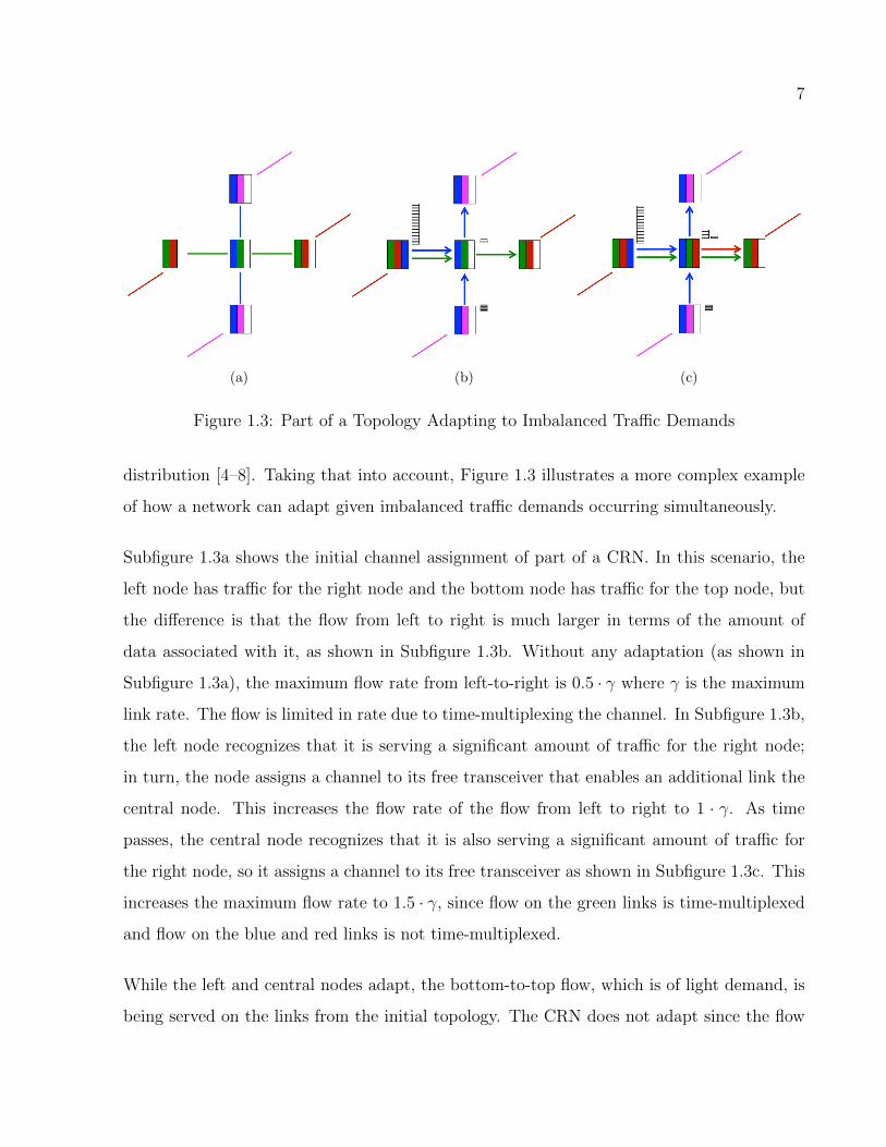
Figure 1.3: Part of a Topology Adapting to Imbalanced Traffic Demands

distribution [4–8]. Taking that into account, Figure 1.3 illustrates a more complex example

of how a network can adapt given imbalanced traffic demands occurring simultaneously.

Subfigure 1.3a shows the initial channel assignment of part of a CRN. In this scenario, the

left node has traffic for the right node and the bottom node has traffic for the top node, but

the difference is that the flow from left to right is much larger in terms of the amount of

data associated with it, as shown in Subfigure 1.3b. Without any adaptation (as shown in

Subfigure 1.3a), the maximum flow rate from left-to-right is 0.5 · γ where γ is the maximum

link rate. The flow is limited in rate due to time-multiplexing the channel. In Subfigure 1.3b,

the left node recognizes that it is serving a significant amount of traffic for the right node;

in turn, the node assigns a channel to its free transceiver that enables an additional link the

central node. This increases the flow rate of the flow from left to right to 1 · γ. As time

passes, the central node recognizes that it is also serving a significant amount of traffic for

the right node, so it assigns a channel to its free transceiver as shown in Subfigure 1.3c. This

increases the maximum flow rate to 1.5 · γ, since flow on the green links is time-multiplexed

and flow on the blue and red links is not time-multiplexed.

While the left and central nodes adapt, the bottom-to-top flow, which is of light demand, is

being served on the links from the initial topology. The CRN does not adapt since the flow

8

demand is light. The point is that CRN intelligently deciphers the traffic characteristics and

channel conditions and adapts the channel assignment to support the high demand flows.

1.4 Problem Definition

We focus on the assignment of channels to each node’s transceivers across the CRN. The

channel assignment induces a multi-channel topology on which network traffic can flow.

Depending on the CRN’s channel assignment, the topology has a certain level of connectivity

and supports a certain capacity.

The primary objective of this work is to design channel assignment strategies to maintain the

multi-channel topology that best suits the network’s traffic flows, which are dynamic, while

maintaining network connectivity. We assume that each node is equipped with multiple

transceivers, each of which can be dynamically tuned to operate on a different channel.

Although node transceivers are able to change channels, they are not able to switch channels

in packet-time, so receiving and forwarding on different channels with a single-transceiver is

not possible. The channel assignment strategies we focus on address capacity maximization

of the current, substantial network flows.

We focus on the scenario where each node has multiple transceivers, with each transceiver

capable of transmitting or receiving on any single channel at a time. The CRN’s channel

assignment must maintain a connected, multi-channel network. Although using a greater

number of transceivers can yield higher network connectivity, there is a cost in terms of

energy consumption for operating each transceiver.

Also, while recognizing the need for assigning transceivers to maintain network connectivity,

the CRN should also be adaptive to the dynamic traffic conditions. To handle heavy traffic

demands and alleviate network congestion, the CRN can enable additional links through

9

channel assignment of the transceivers that are not dedicated to maintaining network con-

nectivity on an as-needed basis, but the benefit for improving flow utility should outweigh

the cost of the additional transceiver allocations.

1.5 Research Contributions

The primary research contribution is proposing a new method of channel assignment that

incorporates two complementary approaches of channel assignment: traffic-independent (TI)

and traffic-driven (TD) assignment. We propose that some transceivers be enabled and

assigned to a channel independently of traffic conditions and some transceivers be enabled

in response to traffic conditions. The TI assignment is designed to maintain stable, baseline

network connectivity. In contrast, the TD is intended to adapt the network’s topology

(through enabling additional links) to better facilitate the end-to-end flow of traffic. Figure

1.4 illustrates this proposal.

We propose that a minimum number of transceivers be assigned independently of traffic

conditions in order for the network to be more flexible in its adaptation to traffic demands.

By conserving resources initially with the TI assignment, the network has more resources for

any TD assignment, and more resources allocated in the TD assignment possibly translates

into higher end-to-end flow rate.

We show the fundamental tradeoffs in the proportion of resources allocated independently of

traffic conditions and in response to traffic conditions. We develop centralized and distributed

heuristic approaches for TI assignment. Also, we develop a distributed TD assignment scheme

where nodes organically adapt the topology to best suit the current traffic conditions. Finally,

we show how this assignment method can be applied with a realistic traffic model, based on

network measurements, that varies flow demand, following a heavy-tailed distribution.

10

Figure 1.4: Two-stage Approach to Traffic-aware Channel Assignment: In stage 1, the CRN

performs TI channel assignment to maintain network connectivity over multiple channels

(colors represent channels, solid lines represent links resulting from TI assignment). In stage

2, the CRN performs TD channel assignment where the CRN senses the traffic conditions as

well as transceiver and channel usage and assigns additional channels enabling additional links

to better support traffic flows (dashed lines represent links resulting from the TD assignment).

When traffic conditions change, stage 2 is repeated, with the TI topology and the new set of

flows as inputs.

11

1.5.1 Balance of TI and TD Resource Allocation

In our first contribution, we examine the fundamental tradeoff in the proportion of resources

allocated independently of traffic conditions and those resources allocated in response to

traffic conditions. As more resources are allocated independently of traffic conditions, the

network can achieve higher connectivity, but as more resources are allocated in response

to traffic demands, the network can support higher end-to-end flow rate. The goal is to

investigate what resource allocation best balances both the desire for maximizing flow rate

and the need for the network to be adequately connected.

Following from Figure 1.4, we formulate the problem as a two-stage, mixed-integer linear

program (MILP), with the first stage being a TI assignment and the second stage being a

TD assignment. In the first (TI) stage, connectivity is maximized using a proportion of the

network’s transceivers. The connectivity-maximization problem is denoted CM(α) where α

is the proportion of the network’s transceivers allocated traffic-independently. In the second

(TD) stage, channels are assigned using the 1−α proportion of the network’s transceivers to

maximize end-to-end flow rate for a given set of flows. The TD flow-maximization problem

is denoted as problem FM.

We find that connectivity increases monotonically as a function of α, but beyond a cer-

tain point there are diminishing returns in terms of additional network connectivity gained

through the allocation of additional transceivers for connectivity. Also, we see that the max-

imum achievable end-to-end flow rate decreases monotonically as a function of α, but beyond

a point the flow rate diminishes more quickly. We find that, at the values of α for which

the network graph is connected, there is little, if any, decrease in flow rate as compared to

the theoretical maximum flow rate when α = 0. These results support our central idea of

a resource-minimized TI assignment followed by a TD allocation. This contribution follows

from our work in [9] and is described in Chapter 3.

12

1.5.2 Resource-Minimized TI Channel Assignment

In our second contribution, we examine the problem of TI channel assignment and develop

a set of approaches that follow our proposal of a resource-minimized TI assignment. Our

approach is in contrast to much of the research literature, which focuses on a strategy of

assigning channels to all available transceivers with the typical objective of either maximiz-

ing connectivity or minimizing interference. However, we compare our approach to other ap-

proaches in the research literature that minimize the resources allocated traffic-independently

to some degree.

The motivation for a resource-minimized TI approach is two-fold. The first motivation is

that energy is conserved, since there is a non-negligible cost in energy for each transceiver

that is activated and tuned to a channel. The second motivation, as outlined previously, is

that, by initially conserving resources, there can be a stronger dynamic response to changing

traffic stimuli through subsequent enabling of and channel assignment to transceivers.

We formulate an optimal approach to resource-minimized TI assignment, with problem RM,

which follows an MILP. We then develop two heuristic algorithms. One is centralized, while

the other is distributed. We find that our proposed approaches perform much closer to

optimal than other proposed approaches in the research literature in terms of the number of

channel assignments necessary to maintain network connectivity.

To fairly compare each TI scheme’s impact on flow rate, problem FM is solved to assign

any transceivers not assigned traffic-independently to maximize flow rate. We find that our

proposed approaches are able to achieve a higher maximum flow rate than other approaches

due to using fewer transceivers for TI channel assignment. Furthermore, our proposed ap-

proaches achieve a flow rate within a small percentage of the optimal (the solutions of both

RM and FM), averaged across all evaluated scenarios. This contribution is an extension

from our work in [10] is described in Chapter 4.

13

1.5.3 Traffic-driven Channel Assignment

In our third contribution, we examine the problem of TD channel assignment. Closely aligned

with the ideals of cognitive networking, we propose an approach that senses traffic condi-

tions as well as channel and transceiver usage and intelligently adapts the channel assignment

locally to better support the end-to-end flow of traffic. The goal is for nodes to act inde-

pendently and organically adapt the topology over time in a way that maintains network

connectivity but optimizes the topology based on the flow demand.

We develop an approach in which nodes each run a background process that aggregates traffic

statistics over a sliding window of time, giving each node the ability to sense which flows are

most substantial. Then, the process senses if any of the substantial flows are bottlenecked

and assigns channels locally to alleviate any bottlenecks if possible. The motivation for not

optimizing based on all flows is that there is a non-negligible cost in terms of energy to

enabling a transceiver and tuning it to a channel, so the benefit of making an adaption to a

flow of light demand (e.g., a one-packet flow) is not worth the cost of enabling and assigning

a transceiver. We argue that light flow demands can be easily served using the resources

dedicated for maintaining network connectivity assigned traffic-independently.

We develop an event-driven simulation to showcase how the resource-minimized TI allocation

scheme, complemented with the distributed, iterative TD allocation scheme, performs in an

event-driven scenario. We show that the distributed TD approach performs close to the

optimal approach in the majority of the evaluated scenarios in terms of flow rate and flow

completion time. Also, the distributed, resource-minimized TI approach complemented with

the iterative, distributed TD approach greatly outperforms the common approach of assigning

all channels independently of traffic conditions. Lastly, we find that our combined distributed

TI-TD approaches enables and disables fewer transceivers while adapting the topology than

the optimal approach by an order of magnitude. This contribution is described in Chapter 5

and follows from our first attempt at a similar problem in [11].

14

1.6 Organization

The remainder of this dissertation is organized as follows. Chapter 2 presents an overview of

the related work in this area. Chapter 3 provides the problem formulation of our proposed

approach for traffic-aware channel assignment and examines the fundamental tradeoff in the

balance of resources allocated traffic-independently and resources allocated in response to

traffic demands. Chapter 4 outlines various traffic-independent (TI) channel assignment ap-

proaches while introducing our proposed resource-minimized approach. Chapter 5 provides

our approach to traffic-driven (TD) channel assignment and presents the performance eval-

uation of the overall proposed scheme. Chapter 6 discusses our main conclusions and areas

for future work.

Chapter 2

Literature Review

In this chapter, we broadly classify related works into three categories: (1) traffic-independent,

(2) traffic-driven, and (3) traffic-aware resource allocation for multi-channel, multi-transceiver

operation in wireless networks. The TI resource allocation schemes allocate all of their re-

sources independently of traffic conditions. Typically, such schemes aim to maximize connec-

tivity or minimize interference. Proposals of TD resource allocation only allocate resources in

response to traffic demands, without dedicating any resources to maintaining basic network

connectivity. Traffic-aware schemes allocate some resources to maintain network connectivity

and some resources in response to traffic demands.

The main contribution of our work, as will be shown in subsequent chapters, is proposing

a traffic-aware approach. Some of the research literature adopts this approach as well, but

these works typically focus on link-level rendezvous and lack a real end-to-end, networking

solution.

2.1 Traffic-independent Resource Allocation

In this section, we discuss related work that allocates resources independently of traffic

conditions. Typically, these approaches focus on the channel assignment of node transceivers

15

16

or network interfaces to form a connected topology. We focus our literature review on TI

assignment schemes that require both ends of a communication link to have a transceiver or

radio dedicated to a common channel.

We categorize approaches as either focusing on maximizing connectivity or minimizing inter-

ference. Table 2.1 presents a summary of the noteworthy TI approaches from the research

literature. We review these approaches in this section, and in Chapter 4 we propose another

approach in Chapter 4 and evaluate it against a subset of the approaches from this section.

2.1.1 Maximize Connectivity

A common approach to the problem of channel assignment in the research literature is to

maximize the network’s connectivity. The main constraint with this approach is to limit

interference, otherwise every node would simply assign all of its transceivers to same set

of channels. By maximizing the network’s TI connectivity, the network may be robust to

network transients such as node or channel outages.

An approach to channel assignment that maximizes connectivity, known as CogMesh [13],

proposes a channel assignment that creates a network consisting of 2-hop frequency clusters.

Each 2-hop frequency cluster is composed of a single clusterhead and nodes that are neighbors

of the clusterhead which tune one transceiver to a common channel. This algorithm starts

with no initial channel assignment, but during channel selection a node selects the lowest

indexed channel that it can use to join a cluster or become a clusterhead. In order to join

a cluster, a node must be within communication range of a clusterhead. In order to become

a clusterhead on a particular channel, a node must not be within interference range of a

clusterhead.

In [12], we propose a related approach through the formation of maximal cliques or frequency

clusters. The benefit of a topology of cliques is increased medium access control (MAC)

17

Table 2.1: Summary of Node Channel Assignment Algorithms

(V: Set of nodes, E : Set of edges based on communication range, T : Number of transceivers per

node, C: Set of channels)

Assignment Schemes Basic Idea Connectivity Guarantee Running Time

Maximal Clique [12] Maximize number of 1-hop Not guaranteed, typically |V| · T

neighbors on a channel connected

CogMesh [13] Lowest indexed c ∈ C reaching a Yes |V| · T

clusterhead or becoming one

Skeleton Assisted Random assignment of T − 1 Yes (likely on control 2 · |V|

Partition Free (SAFE) transceivers, last transceiver channel)

[14] reaches remaining neighbors

Centralized Tabu- Use a Tabu-search to find Yes O(r · |E|4)

based Algorithm [15] the minimum aggregate (branching parameter r)

interference with connectivity

constraint

Distributed Greedy Iteratively reduce number of Yes O(|E|2 · |C|)

Algorithm (DGA) [15] local interferers with local

connectivity constraint

Distributed Channel Iteratively reduce number of Yes (control channel) O(|V|2 · |C|)

Assignment (DCA) [16] local interferers

Cognitive Spectrum Assign each link to least Not guaranteed, typically O(|V| · |E|)

Assignment Protocol interfering channel connected

(CoSAP) [17]

Interference-aware Find minimal subgraph, assign Yes O(k · |V|3 · log |E|+ |E|2)

Topology control least interfering channel to (k is the k-connectivity

(IA-TC) [18] links in order of lowest conflict of the subgraph)

degree

Connected Low Assign each link to least Yes Complexity is not

Interference Channel interfering channel recursively provided, proven to

Assignment (CLICA) [19] prioritizing links based on num- be NP-complete

ber of unassigned transceivers

Breadth-First Search Assign links of minimum Yes O(|E|2 · T 2 · |C|)

Channel Assignment interference emanating

(BFS-CA) [20] from the mesh gateways

18

efficiency by eliminating hidden terminals. In this approach, nodes start with no initial

channel assignment and sequentially select channels. During channel selection, a node will

choose to join the largest clique possible without becoming an interferer to any node.

Another channel assignment protocol, titled skeleton assisted partition free (SAFE), is pro-

posed in [14]. In SAFE, all nodes seek to reach all neighbors in communication range. As one

contribution, the authors of [14] apply the pigeonhole property to conclude that if 2 ·T > |C|

(where T is the number of transceivers and C is the set of channels), then any channel

assignment with T channels assigned per node results in a network of fully-connected neigh-

borhoods (all nodes in communication range of each other share a common channel). As

another contribution, in [14] the SAFE algorithm is proposed. It uses a (uniformly) random

assignment of all transceivers if 2 · T > |C|. Otherwise, all but one transceiver are assigned

randomly at first. Subsequently, the last transceiver is assigned a channel reaching all un-

reached neighbors. If no channel reaches all unreached neighbors the last transceiver tunes to

a pre-determined, network-wide default channel. The biggest disadvantage of this approach

is that it is highly dependent on the ratio of channels to transceivers. As the ratio grows, the

number of nodes on the default channel is expected to also grow, causing the default channel

to become congested.

In these approaches, achieving connectivity to each node in the network is equally weighted,

without regard to which nodes have higher traffic demands. Although these approaches

achieve an evenly distributed high connectivity among all nodes, they do not allocate any

resources based on serving the traffic demands. For example, it may be better for the network

for some nodes to have higher connectivity than others if they have to serve high traffic

demands.

2.1.2 Minimize Interference

Another common approach to TI channel assignment is to minimize the network’s aggregate

interference. The main constraint with this approach is maintaining a prescribed level of

19

network connectivity by either enforcing that a connected network graph results or enforcing

that every pair of nodes within communication range of each another is tuned to a common

channel.

A set of approaches that minimize interference are provided in [15]. In [15], a Tabu-search

method is proposed for finding the minimum sum of aggregate interference as seen by all

nodes, with the constraint that all nodes have fully-connected neighborhoods (all nodes

in communication range of one another share a common channel). The first stage of the

approach uses a Tabu-search with branching parameter r for exploring potential neighboring

solutions. It finds a channel assignment that minimizes the degree of the multi-channel

conflict graph (minimizes aggregate interference). The assignment from the first stage ignores

the constraint of the number of transceivers per node, meaning some nodes may have more

than T channels assigned, but in the second stage, a merging operation merges nodes and

edges that violate this constraint. The merging operation chooses merges that minimally

increase the aggregate network interference.

Also, in [15] the authors propose a distributed approach entitled distributed greedy algorithm

(DGA). The channel selection process starts with an initial assignment of only the lowest

indexed channel. DGA prescribes continuously choosing the channel (re-)allocation at each

node that results in the maximum decrease in the number of interferers, while maintaining

fully connected neighborhoods at all times. Another similar approach is proposed in [16],

with the difference that fully connected neighborhoods are not required, which makes this

algorithm sensitive to the number of channels because there is no constraint (or objective)

that assures (or strives for) network connectivity.

In another approach, entitled cognitive spectrum assignment protocol (CoSAP) [17], each

node continually selects neighboring nodes without a channel in common to form links with.

Once the node initiating the link formation has selected a node to form a link with, a channel

is selected by the two nodes forming the link. If both endpoints have a free transceiver, they

pick any channel so as to minimize the aggregate number of interferers as seen by both nodes.

20

If one endpoint does not have a free transceiver, the other endpoint picks a channel already

selected by the first endpoint with the minimum number of interferers.

In [18], an approach called Interference-Aware Topology Control (IA-TC) is proposed. In the

first step of IA-TC, the authors propose a topology control scheme called Minimal Interference

Survivable Topology Control (INSTC) that selects a threshold of minimal conflict weight

where the set of edges below the threshold connect the graph and will subsequently be

assigned channels. In decreasing order of conflict weight, the edges are greedily assigned the

least used channels in interference range. Depending on the problem parameters, some nodes

may have unassigned transceivers. In [18], these unassigned transceivers are assigned the

least used channel in the node’s interference range in the last step.

In [19], a channel assignment algorithm titled Connected Low Interference Channel Assign-

ment (CLICA) is proposed. The algorithm takes as input a graph (with edges assigned

channels). Similar to IA-TC the edges are assigned channels that are in minimal use within

interference range; however, the order in which edges are assigned adapts based on how many

transceivers remain at each node. The nodes with only a single unassigned transceiver are

given the highest priority to be assigned next. The resulting channel assignment assigns

channels to all edges.

In [20], the authors adopt a mesh networking scenario in which interference is also minimized,

but in this scenario links are assigned channels according to a breadth-first search approach

emanating from the mesh gateways1. The channel for each link is chosen based on minimizing

interference.

1Gateways in a mesh networking scenario are defined as a member of the network for non-gateway nodes

to get their traffic serviced through reaching a broader network (i.e., the internet). Gateways use a different

set of resources to reach the broader network.

21

2.1.3 TI Dual Problem Relationship

These two approaches to TI channel assignment are related in that both formulate the

problem with considerations of network connectivity and interference. In the connectivity-

maximization approach, connectivity is maximized with the constraint of having limited

interference. This is in contrast to the interference-minimized approach, where aggregate

interference is minimized subject to achieving a certain level of connectivity.

Depending on the functions for determining connectivity and interference on the network

graph and the problem’s parameters (i.e., number of nodes, transceivers, channels, etc.), both

approaches could yield identical optimal solutions to channel assignment, and the relationship

of such problems is often categorized as a dual problem relationship. Depending on the

adopted definition of dual problem relationship, dual problems can represent various ideas.

We categorize two problems as duals when the criteria of the objective function and one of

the problem’s constraints are interchanged, as well as the polarity of the objective function.

This definition is similar to the definition of dual problems in a pair of linear programs (LPs).

This dual problem characteristic of these approaches is noteworthy because it suggests that

the TI approaches that either maximize connectivity or minimize interference in the research

literature are more similar in nature than at first glance, since an optimal approach of each

could yield the same solution.

2.2 Traffic-driven Resource Allocation

In contrast to TI allocation schemes, there is a set of research literature focussed on TD

allocation which allocates resources in response to traffic stimuli. Works of this nature

tend to assume underlying network connectivity and, in many cases, global knowledge and

centralized control.

22

We categorize two sets of research literature on TD allocation. One set of these approaches

focuses on the link-channel assignment problem. Specifically, they propose assigning channels

to links (each with traffic demands) with the objective of maximizing the number of simul-

taneous link transmissions among multiple channels. Another set of approaches proposes

optimal channel assignment, scheduling, and routing to maximize end-to-end flow rate in a

multi-hop scenario.

2.2.1 Link-Channel Assignment Scheduling

In this problem setting, the goal is to schedule the maximum number of transmissions across

multiple channels. Channels are assigned to the set of links (with each link assumed to have

traffic to serve). The objective function in this problem setting is maximizing the number of

successful transmissions while secondarily minimizing aggregate transmit power. Table 2.2

presents a summary some common approaches from the research literature.

In [21], it is proposed that links be sequentially assigned to the channel with lowest interfer-

ence if it is sensed to be below a predetermined interference threshold. Also, the proposal in

[21], proposes setting the transmit power of the link to a predetermined power level above

the target signal-to-interference-noise ratio (SINR) to prevent other subsequently admitted

co-channel links from interfering excessively and lowering the SINR below the target. This

approach is sensitive to the predetermined interference threshold and the predetermined

power level above the target SINR.

In [22], another scheme is proposed where channels are selected at random from the set of

channels that are unused within a predetermined distance. The power control in [22] is an

improvement upon the power control phase as compared to [21] by introducing an iterative,

distributed power control phase that allows links to increase their transmit power as necessary

to avoid falling below the SINR threshold. Furthermore, in [26] it is demonstrated that the

transmit power adaptations of the links converge.

23

Table 2.2: Summary of Link Channel Assignment Algorithms

(L: Set of links with traffic, C: Set of channels)

Assignment Schemes Basic Idea Running Time

Least Interfering Channel and Sequentially assign links to channels with the lowest O(|L| · |C|)

Power Assignment [21] interference, set the power according to the minimum

acceptable SINR

Spatial Channel Separation and Sequentially assign links to channels that are unused within O(|L|2)

Iterative Power Assignment [22] a predetermined distance, iteratively adjust transmit power

to maintain a given target SINR

Least Interfering Channel and Sequentially assign links to channels with lowest interference, O(|L|2)

Iterative Power Assignment [23] iteratively adjust transmit power to maintain a given target

SINR

Minimum Power Increase Sequentially assign the link to the channel that requires the O(|L|4 · |C|)

Assignment [24] minimum aggregate increase in network transmit power (to

maintain acceptable SINR levels) on the assigned channel

Conflict Graph Assignment [25] Sequentially assign the set of links of maximum cardinality to O(|L|2 · |C|2)

a single channel such that all links can meet SINR require-

ments on the channel after an iterative power assignment

24

In [23], we propose combining the channel selection of [21] and the iterative power control

approach of [22]. As compared to the approaches of [21] and [22], this improves the number

of links that can be scheduled in the network and in some cases uses a lower average transmit

power per link.

In [24], a centralized algorithm is proposed where global knowledge of cross-link power gains

is used to assign channels. The basic idea is to assign a link to the channel that causes the

minimum increase in aggregate transmit power of the other co-channel links. Other links

increase their transmit power to maintain a target SINR. In [23], we find that although

this approach is more computationally complex, it yields the highest number of scheduled

transmissions and uses the lowest average transmission power as compared to all of the

aforementioned approaches.

Another approach proposed in [25] uses a weighted conflict graph which is based on cross-link

power gains to perform a greedy assignment. The approach finds the maximum number of

unassigned links that can be supported on each channel. The channel that can support the

most links is used for those links. The process iterates on all channels. In [23] this approach

did not perform as well as the approach of [24] in terms of number of transmissions or average

power per link, but it did outperform the other aforementioned approaches in [21–23].

In this problem setting, all resources are allocated to the set of network links (all of which are

assumed to have traffic). There is no allocation of resources providing network connectivity.

Also, the channel assignment is not correlated from one time slot to the next. This leads to

high frequency of channel switching of nodes’ transceivers.

2.2.2 Channel Assignment, Scheduling, and Routing

Another type of resource allocation examined in many popular works proposes traffic-driven

(TD) assignment strategies for maximizing end-to-end flow rate through channel assignment,

25

scheduling, and routing. However, like the link-based assignment schemes, these schemes

typically assume a zero-cost control plane enabling underlying network connectivity and

lack consideration of practical CR limitations that may impact network connectivity. These

constraints include a limited number of transceivers per node, non-negligible costs associated

with enabling and tuning a transceiver to a channel, and non-negligible channel-settling

times. Works of this nature also typically assume a time-slotted setting with transceivers

that can change channels in each slot.

In [27], an approach typically referred to as back-pressure is proposed. This approach makes

forwarding decisions based on the queue-length differential, where packets are forwarded to

nodes with less traffic in their queue. This approach is shown to be flow-rate optimal. In [28],

a variant of back-pressure is proposed where forwarding decisions are based on minimizing the

transmission distance (to minimize transmit power). In [28], they show that this approach

has the tradeoff of increased delay for savings in transmit power. Back-pressure is extended

to the mesh networking scenario in [29]. In [29], each node maintains a collision queue and

is granted higher probability of transmitting to the mesh gateway if it experiences multiple

collisions. This provides guarantees for user fairness and network stability.

Maximizing flow rate with back-pressure schemes can lead to high delay due to the utilization

of long paths [30]. In [30], a variant of back-pressure is proposed where there is a favorable

tradeoff between maximum flow rate and delay. In [30] flow rate is traded for significantly

reduced delay by not selecting excessively long routes to the destination as traditional back-

pressure tends to do.

In [31], another approach is proposed where flow rate is maximized by solving the problem of

joint channel assignment, routing, and link scheduling without the assumption of transceivers

that can change channels on a per-packet basis. In [31], a centralized algorithm is provided

that achieves within a constant factor of the optimum. A related approach is proposed in

[32] where the focus is on the scheduling as many links as possible to serve traffic flows over

multiple channels. Similar to back-pressure techniques, in [32], they make use of queue-length

26

differentials to set up new end-to-end routes. Also, in [32] an adaptive distributed algorithm

is presented that is proven to perform within a fraction of the optimal. In contrast to [31],

in [32] it is assumed that each node has a receiver dedicated to every channel, so nodes can

receive on all channels simultaneously.

In [33], a similar problem is solved with the addition of transmit power considerations. In [33],

a new a metric is developed that is called bandwidth-footprint product (BFP) which refers

to the area affected (its footprint) by a transmitter. By minimizing transmit power with

a fixed channel bandwidth, the BFP is minimized along with interference to neighboring

communications sessions, which is shown in [33] to increase flow rate. In contrast to the

approaches proposed in [31] and [32], the approach in [33] allows channel switching on per-

packet basis. Also in [33], a distributed approach is shown to perform within a small fraction

of the optimum in the majority of simulation trials.

All these approaches allocate resources in a TD manner, and each is shown to perform

comparably to their respective optimal problem formulations. However, these schemes do

not address the practical issue of network connectivity. In [32], it is recognized that an area

for future work includes issues for real implementation where they must address many issues

related to the exchange of information (e.g. queue-length differentials, channel schedules,

etc.). In a wireless networking scenario, this is a cause of major concern since the flow of

control traffic must utilize the same resources that are used for user traffic. This is the main

motivation for our primary contribution in the examination of optimizing the topology while

maintaining basic network connectivity.

2.3 Traffic-aware Resource Allocation

In this section, we discuss related works on traffic-aware resource allocation. These ap-

proaches provide network connectivity and allocate some resources with considerations of

traffic conditions.

27

Table 2.3: Summary of Multi-channel MAC protocols

Protocol Neighbor Discovery Data Exchange Setup Synch Ch Sets

Multi-Channel MAC [34] Assumed Hop to receiver & RTS/CTS Mild Static

Cognitive MAC [35] On control channel Schedule NAV High Dynamic

Dedicated Ctrl Channel [36, 37] On control channel RTS/CTS on ctrl channel None Static

Common Hopping [18, 38, 39] Assumed RTS/CTS on current hop Mild Static

Sequence-based Rendezvous [40] Blind discovery Not protocol specific Mild Static

Slotted Seeded Channel Hopping [41] Assumed Wait for hop Mild Static

Split Phase [42] On control channel Schedule NAV Mild Static

On-Demand Channel Switching [43] Mildly Assumed Multi-channel RTS/CTS None Static

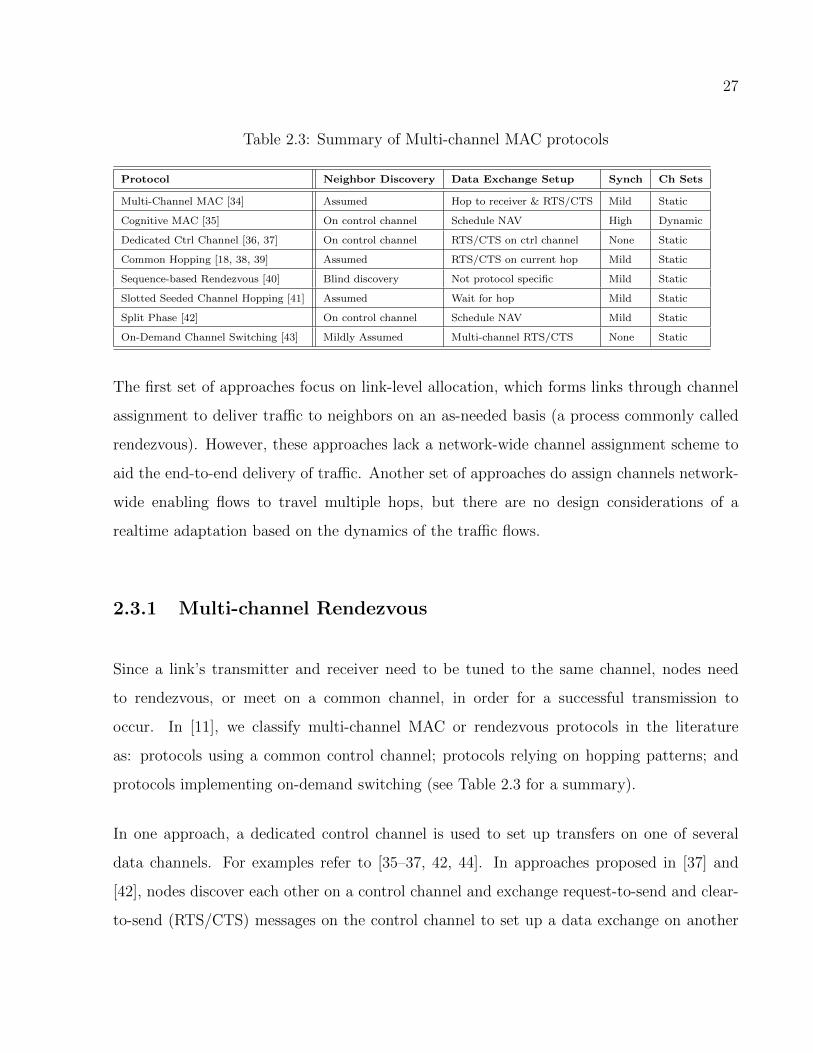
The first set of approaches focus on link-level allocation, which forms links through channel

assignment to deliver traffic to neighbors on an as-needed basis (a process commonly called

rendezvous). However, these approaches lack a network-wide channel assignment scheme to

aid the end-to-end delivery of traffic. Another set of approaches do assign channels network-

wide enabling flows to travel multiple hops, but there are no design considerations of a

realtime adaptation based on the dynamics of the traffic flows.

2.3.1 Multi-channel Rendezvous

Since a link’s transmitter and receiver need to be tuned to the same channel, nodes need

to rendezvous, or meet on a common channel, in order for a successful transmission to

occur. In [11], we classify multi-channel MAC or rendezvous protocols in the literature

as: protocols using a common control channel; protocols relying on hopping patterns; and

protocols implementing on-demand switching (see Table 2.3 for a summary).

In one approach, a dedicated control channel is used to set up transfers on one of several

data channels. For examples refer to [35–37, 42, 44]. In approaches proposed in [37] and

[42], nodes discover each other on a control channel and exchange request-to-send and clear-

to-send (RTS/CTS) messages on the control channel to set up a data exchange on another

28

channel. Approaches proposed in [36] and [35] make use of a network allocation vector (NAV)

that notifies other nodes of the length of the transmission. The use of a common control

channel simplifies rendezvous. In [44], an end-to-end routing scheme is developed using the

metric of estimated transmissions time (ETT) which takes into account switching times of

802.11 systems. A major drawback is that the control channel can become congested or

unavailable due to a primary user and possibly lead to underutilization of the data channels.

Another drawback is that a transceiver is dedicated for control purposes for at least a portion

of a duty cycle.

Common hopping protocols rely on devices hopping on various channels along with one

another in a common hopping pattern. In this approach nodes are assumed to know each

other’s hopping pattern. Nodes exchange RTS/CTS messaging on a channel they are tuned

to and remain on the channel until the transfer is complete. Examples include [18, 38, 39]. A

common hopping pattern precludes the need for a common control channel. A disadvantage

is that synchronization is necessary. Achieving synchronization is not trivial, yet assumed in

many MAC protocol designs. Also, frequently switching channels may be inherently costly

in terms of energy consumption and radio settling time, possibly decreasing the effectiveness

of this approach.

Instead of having a community hopping pattern, devices can have their own hopping sequence.

Examples include [34] and [41]. The improvement over having a common hopping pattern is

that multiple rendezvous can happen simultaneously on orthogonal channels [45], but devices

must obtain neighboring hopping patterns. In [34], So proposes that the transmitting node

change channels to meet the receiver on its hopping sequence. In [41], Bahl proposes nodes

wait to transmit until their hopping sequences overlap and nodes stay on the channel until the

transmission has completed. In [40], each node employs a hopping sequence that minimizes

the expected number of hops to rendezvous with other nodes. The advantage of such an

approach is that nodes are not required to exchange hopping sequences.

29

In [45] Mo finds that if the channel switching penalty is below some threshold, using inde-

pendent hopping sequences improves throughput. Since switching channels costs a device

time and power, the on-demand channel switching (ODC) protocol [43] provides a way to

utilize multiple channels without synchronization. The basic approach is for the transmitter

to search for the receiver and attempt to set up a transmission by sending RTS messages

on multiple channels. This approach may reduce channel switching as compared to using a

hopping sequence, but it may make rendezvous more difficult as the list of available channels

grows.

In these approaches some resources are dedicated to maintaining network connectivity and

other resources are allocated on an as-needed basis to serve traffic demands. These approaches

focus on a link-level allocation lacking a natural end-to-end extension.

2.3.2 Multi-hop, Mildly Traffic-aware Assignment

Another set of approaches allocate resources taking into account channel assignment consid-

erations from source to destination over multiple hops. In contrast to the TD allocations

schemes presented in Section 2.2, these schemes do allocate resources providing network con-

nectivity. However, the schemes presented in this subsection are not as well-equipped to

react to changing traffic demands as are the purely TD schemes.

The approach presented in [46] is designed for a mesh networking scenario where traffic flows

to mesh gateway nodes. The basic idea for the approach is to rank the nodes in terms of their

expected amount of traffic and their distance (in terms of hop count) away from the nearest

gateway, and links are assigned channels of minimal interference in order of their rank, which

makes this approach similar to [20], since the ranking is influenced by the hop-count away

from the gateway node.

A similar approach in [47] calls for interference minimization, with links of higher measured

(or estimated) load having higher priority to being assigned channels of lower interference.

30

Also, the proposal in [47] accounts for changing link loads based on adjusting the channel

assignment (e.g. some routes may become more attractive than others in terms of interference

and, in turn, are given more load). The proposed approach attempts to converge to a stable

channel assignment (and thus link loading) over time.

Although both approaches proposed in [46] and [47] allocate resources based on traffic con-

ditions, they do not adopt a dynamic model as do the TD schemes discussed in 2.2. In [46],

the authors show that their channel assignment converges when given a single traffic profile

after 40 seconds in a simulation environment. In [47], the scheme is designed to adapt the

network’s channel assignment to changing conditions on the order of hours or days. Clearly,

these approaches are not designed to handle bursts of traffic. We focus our adaptation scheme

to be on a much shorter time scale.

2.4 Summary

In this chapter, we outlined related research literature on traffic-independent, traffic-driven,

and traffic-aware resource allocation. Traffic-independent resource allocation schemes focus

on allocating all resources to establish a desirable topology, in terms of connectivity and

interference. These schemes do not incorporate any allocation that is responsive to traffic

demands.

Research literature on TD resource allocation focuses on adapting the channel assignment

to meet the traffic conditions; however, there are not any resources dedicated to establishing

basic connectivity. This leads to a topology without any stable components, causing it to

react on any traffic demands, even light traffic demands.

We recognize the importance of both ideas, and highlight some research literature that incor-

porates dedication of resources in both a TI and TD manner. However, such approaches lack

31

an end-to-end scope or lack the ability to adapt to dynamic traffic conditions such as burst

traffic demands. The contribution of this document is in a proposal of a fully distributed

traffic-aware resource allocation that takes into account network-wide impacts and can allo-

cate resources to handle burst traffic demands while maintaining network connectivity.

Chapter 3

Balance of Traffic-independent and

Traffic-driven Allocations

In Chapter 2, we categorized three themes to resource allocation in multi-channel networking:

completely traffic-independent (TI) in Section 2.1, completely traffic-driven (TD) in Section

2.2, and traffic-aware (TA) resource allocation in Section 2.3. In this chapter, we outline an

end-to-end, dynamic TA resource allocation, which has a resource-minimized, TI assignment

component complemented with a TD resource allocation of the remaining resources. The

TD allocation is dynamic and based on the current, active traffic demands.

The TA allocation scheme is the main focus of this dissertation. The TA channel assignment

scheme addresses both goals of (1) supporting baseline network connectivity and (2) allowing

the network to adapt, pursuing end-to-end goals of flow rate maximization. We argue that

these two design goals of a channel assignment scheme must be addressed together, since

they both access the same pool of resources. An assignment scheme of one type of allocation

limits the actions and effectiveness of the other. The objective is to balance the need for a

stable baseline topology and the desire to maximize flow rate by dynamically adapting the

topology to current network conditions.

32

33

Our proposed TA allocation scheme offers a more balanced allocation of resources as com-

pared to much of the research literature, since our scheme dedicates resources to maintain-

ing network connectivity while allocating other resources in response to changing network

demands. The completely TI allocation schemes from the research literature dedicate all re-

sources to maintaining network connectivity and are not responsive to traffic demands. This

is in contrast to the TD schemes from the research literature, which allocate resources only

in response to traffic demands and lack an allocation of resources dedicated to maintaining

network connectivity.

In this chapter, we highlight the favorable tradeoffs for adopting the TA allocation scheme

as opposed to a completely TI or completely TD approach. Also, we explore the fundamen-

tal tradeoffs in the amount of resources allocated traffic-independently and the amount of

resources allocated in response to traffic demands. The goal is to find a resource allocation

that meets the need of a stable baseline topology and the desire to maximize flow rate. This

type of allocation follows the ideas of cognitive networking [2] where the network continu-

ously senses its operating conditions and traffic demands and adapts its resource allocation

appropriately.

The evaluation in this chapter presents a broad comparison of the TA approach against TI

and TD approaches. We formulate a two-stage, mixed-integer linear program (MILP) of the

TA assignment scheme, as well as a two-stage MILP representing TI and TD assignment

schemes. We use these formulations to evaluate the soundness of the TA approach compared

to approaches that are purely TI or TD and to explore the fundamental tradeoffs involved.

The contributions of this chapter are as follows. In section 3.1, we formulate the fundamental

problem we address throughout the dissertation of a TA assignment that both maintains net-

work connectivity and adapts to traffic demands. In section 3.2, we describe our numerical

analysis and provide our results. We show that the TA scheme can achieve the desired charac-

teristics of both TI and TD allocation schemes without any major shortcomings. Specifically,

the TA approach supports significantly higher flow rate than a TI approach while using fewer

34

Figure 3.1: Two-Stage MILP Approach: colors represent channels, solid and dashed lines

represent TI and TD links, respectively.

transceivers in aggregate across the network. Also, the TA approach is able to support com-

parable flow rates as those of a TD scheme, while maintaining network connectivity in the

majority of the scenarios that we evaluate. In subsequent chapters, we propose a set of al-

gorithms and methods outlining how our TA approach could work in a decentralized fashion

without relying on an optimal, centralized controller.

3.1 Problem Formulation

We formulate the problem as a two-stage MILP of channel assignment and flow routing.

Figure 3.1, which is identical to Figure 1.4 of Chapter 1, shows the basic idea of the two-stage

MILP. The first stage is the TI stage where channels are assigned, inducing a topology that

does not change based on traffic conditions. The second stage is the TD stage where channels

are assigned to any unused transceivers from the TI stage, based on traffic conditions, with

the goal of maximizing throughput by modifying the topology to be more suited to the current

traffic demand. Under changing traffic conditions, the topology can be re-optimized to meet

35

the current traffic demands. In this section, we define the two-stage MILP that models the

TA approach. Subsequently, we define another two-stage MILP that is used for comparison

in our evaluation against other types of resource allocation schemes.

3.1.1 Two-stage, Traffic-Aware (TA) MILP

As our main contribution, we promote a TA approach that allocates minimal resources in the

first (TI) stage, with the goal of using as few transceivers as possible to create a connected

topology, leaving as many unassigned transceivers as possible to optimize the topology based

on traffic characteristics in the second (TD) stage. In the following subsections, we provide

the details of the two-stage formulation.

3.1.1.1 Resource-minimized, TI Stage: Problem RM

Starting with physical layer constraints, we assume the available spectrum is divided into

orthogonal channels contained in set C, and each transceiver occupies a single channel at

any given time. Although radios can occupy any channel, we assume the cost of channel

switching is too high to incur on a per-packet basis, so nodes cannot receive on one channel

and transmit on another with the same transceiver. Nodes are contained in set V . Problem

RM’s objective function is

min∑i∈V

|Ci|, (3.1)

where Ci is the set of channels tuned to by node i with its transceivers. Each node is equipped

with T transceivers, so each node can occupy up to T channels. That is,

|Ci| ≤ T (∀i ∈ V). (3.2)

Also, we define Cij = Ci ∩ Cj as the set of channels nodes i and j have in common.

36

The communication and interference model we adopt for this problem is the double-disk

model similar to [10, 13, 15, 18, 19]. There are two disks centered at each node. The inner

disk, the communication range disk, has a radius of rcomm and the outer disk, the interference

disk, has a radius of rint (rcomm < rint). A node i can communicate with any node j within

its communication range if Cij 6= ∅. If node j is within node i’s interference disk and Cij 6= ∅,

nodes i and j interfere with one another. By definition if two nodes can communicate with

each other, they can interfere with each other as well.

We represent the double-disk relationships with sets CRi and IRi as the set of nodes within

communication range and interference range respectively. We also define binary matrices

as follows. The interference range matrix is IR, where IR[i][j] = 1 if node i ∈ IRj and 0

otherwise. Similarly, we define the communication range matrix CR[i][j] = 1 if node i ∈ CRj

and j are in communication range and 0 otherwise. If CR[i][j] = 1, then IR[i][j] = 1 by

definition.

We define communication graph G(V , E) where E is the edge set. An edge eij exists in E if

Cij 6= ∅ and CR[i][j] = 1. We define set Pij as the set of all paths between node i and j,

where a path pij is a list i, eik, k, ekl, l, ... , m, emj, j of nodes and edges where no node

or edge repeats. Since we are trying to achieve basic network connectivity using minimal

resources, we stop allocating resources once there is a path between all node pairs in the

graph. That is,

|Pij| ≥ 1 (∀i ∈ V ,∀j ∈ V). (3.3)

For the first (TI) stage of the MILP, we seek a channel assignment that results in a limited

number of interferers (β) for each node. That is,∑j∈V,j 6=i

(IR[i][j]− CR[i][j]) · |Cij| ≤ β (∀i ∈ V). (3.4)

Note that under certain conditions (e.g. a low value of β, a particularly awkward node

placement, few transceivers, and/or few channels) this constraint can cause the problem to

37

be infeasible. We set β = 0 in our numerical analysis throughout the dissertation, and we

evaluate scenarios where |C| ≥ 8 and T ≥ 2. This reduces the probability of an infeasible

problem, but if this constraint drives the problem to be infeasible, this constraint could be

relaxed to allow some interferers by setting β > 0. In the scenarios we evaluated, setting

β = 0 did not make the problem infeasible. In Chapter 4, we discuss how β can be relaxed.

The complete RM problem formulation is as follows.

min∑i∈V

|Ci|

subject to

|Ci| ≤ T (∀i ∈ V)

|Pij| ≥ 1 (∀i ∈ V , ∀j ∈ V)∑j∈V,j 6=i

(IR[i][j]− CR[i][j]) · |Cij| ≤ β (∀i ∈ V)

3.1.1.2 Flow-maximized, TD Stage: Problem FM

After the TI stage completes, there is a traffic-independent, resource-minimized, multi-

channel connected topology. Then, in the TD stage, channels are assigned to any radios

not assigned in the TI stage, adapting the topology to maximize flow rate r. We denote the

set of flows as F . Each flow f has a weighting factor of wf , which is used to scale the rate

of each flow with respect to r. The objective function reads

max∑f∈F

wf · r. (3.5)

As in the first stage, we allow each node to occupy up to T (the number of radios per node)

channels. We define lij(c) as the physical layer transmission rate from node i to node j on

38

channel c. We assume each radio has a maximum rate γ for the sum total of transmission

and reception rate per channel. This constraint implies nodes can receive and transmit traffic

on each channel/radio through some sort of time multiplexing. We also limit the aggregate

physical layer link transmission rate on each channel within every interference disk to be

γ. This implies that channel sharing (through time multiplexing) is possible among nodes

co-located in an interference disk. These constraints read as follows.∑j∈V,j 6=i

lij(c) +∑

j∈V,j 6=i

lji(c) ≤ γ (∀i ∈ V ,∀c ∈ Ci) (3.6)

∑j∈V

∑k∈V,k 6=j

ljk(c) · IR[i][j] ≤ γ (∀i ∈ V , ∀c ∈ Ci) (3.7)

Each interference disk region is centered at node i, so the aggregate rate of all transmitters, j,

within range of i is constrained. Note that these constraints do not enforce a strict scheduling;

doing so would make the problem much more difficult to solve.

We constrain the aggregate communication rate of flows between nodes as:∑f∈F

tij(f) ≤∑c∈Cij

lij(c) · CR[i][j] (∀i ∈ V ,∀j ∈ V , j 6= i),

where tij(f) is the data transfer rate for flow f from node i to node j, irrespective of the

set of channels involved. The source and destination nodes for flow f ∈ F are denoted as

s(f) and d(f) respectively. Flow conservation at each intermediate node i ∈ V\{s(f), d(f)},

f ∈ F is stated as,∑j∈V,j 6=i

tij(f) =∑

k∈V,k 6=i

tki(f) (∀f ∈ F ,∀i ∈ V , i 6= s(f), d(f)).

Flow conservation out of each source node i is stated as,∑j∈V,j 6=i

tij(f) = r (∀f ∈ F , i = s(f)). (3.8)

Since there is flow conservation at source and intermediate nodes, there is flow conservation

at the destination node. Lastly, we have non-negativity constraints for flow and link rates,

tij(f) ≥ 0 (∀i ∈ V ,∀j ∈ V ,∀f ∈ F), (3.9)

lij(c) ≥ 0 (∀i ∈ V , ∀j ∈ V ,∀c ∈ C). (3.10)

39

The complete problem formulation for problem FM is as follows.

max∑f∈F

wf · r

subject to

|Ci| ≤ T (∀i ∈ V)∑j∈V,j 6=i

lij(c) +∑

j∈V,j 6=i

lji(c) ≤ γ (∀i ∈ V ,∀c ∈ Ci)

∑j∈V

∑k∈V,k 6=j

ljk(c) · IR[j][i] ≤ γ (∀i ∈ V ,∀c ∈ Ci)

∑f∈F


lij(c) · CR[i][j] (∀i ∈ V ,∀j ∈ V , j 6= i)

∑j∈V,j 6=i

tij(f) =∑

k∈N ,k 6=i

tki(f) (∀f ∈ F ,∀i ∈ V , i 6= s(f), d(f))

∑j∈V,j 6=i

tij(f) = r (∀f ∈ F , i = s(f))

tij(f) ≥ 0 (∀i ∈ V , ∀j ∈ V ,∀f ∈ F)

lij(c) ≥ 0 (∀i ∈ V ,∀j ∈ V ,∀c ∈ C)

Table 3.1.1.2 provides a summary of the notation used in the TA, two-stage MILP defined

in this subsection.

3.1.2 Parameterized Formulation

In this subsection, we provide a similar formulation following the workflow outlined in Figure

3.1. The motivation for this formulation is to evaluate the fundamental tradeoff between the

TI connectivity and flow rate. In this formulation, we exchange the TI stage (RM) for a

40

Symbol Definition

V Set of nodes

E Set of edges

C Set of channels

Ci Set of channels assigned to node i

Cij Set of channels assigned to i and j (Ci ∩ Cj)

T Number of radios per node

γ Maximum capacity of radios, links, and

interference disks

IR[i][j] Binary interference range matrix, 1 if i and j

are in interference range of each other

CR[i][j] Binary communication range matrix, 1 if i and

j are in communication range of each other

eij Edge in edge set E if Cij 6= ∅ and

CR[i][j] = 1

Pij Set of all paths from i to j

lij(c) Transmission rate on link i to j on channel c

F Set of all network flows

s(f), d(f) Source and destination nodes of flow f ∈ F

tij(f) Node-to-node transfer rate of flow f from i to j

r Base rate for all flows

wf Weight of flow f ∈ F

Table 3.1: Summary of Traffic-aware, Two-stage MILP Notation

41

connectivity-maximized TI approach, which we denote as problem CM(α), where α is the

proportion of network transceivers allowed to be assigned traffic-independently (0 ≤ α ≤ 1).

As compared to RM, CM(α) maximizes network connectivity using a specified proportion

of the radios in the network, α, and is the dual problem to RM.1 The second (TD) stage is

unchanged from subsection 3.1.1.2. In this subsection, we define CM(α) and discuss how to

vary α to effectively encompass the existing research literature.

3.1.2.1 Connectivity-maximized (CM), TI Stage

The motivation for this formulation is to evaluate the fundamental tradeoff between the

TI network connectivity and maximum flow rate. The objective is to maximize network

connectivity using no more than α · |V| · T radios.

The usual graph-theoretic metric for graph connectivity is k-node-connectivity, where k is

the minimum number of node-disjoint paths over all node pairs. We denote the number

of node-disjoint paths between nodes i and j as PNDij , which equals the cardinality of the

maximum-sized subset of Pij whose elements, which are paths, have no nodes in common

other than nodes i and j. The drawback of the k-node-connectivity metric is that it is

dominated by the worst node-pairing. We suggest a more granular metric k′, where k′ is k

plus the proportion of all node pairs {(i, j) : i, j ∈ V , i 6= j} with more than k node-disjoint

paths PNDij > k. This is written as:

k′ =1

|V| · (|V| − 1)·∑i∈V

∑j∈V,j 6=i

min(PNDij , k + 1). (3.11)

Note that expression min(PNDij , k + 1) ∈ {k, k + 1} so k′ is in the interval [k, k + 1).

1The objective switches from minimizing the sum of |Ci| terms in RM to maximizing k′ in CM(α). The

constraints of connectivity from RM appear in the objective of CM(α), and the terms from the objective

function in RM (Ci terms) appear in the constraints of CM(α).

42

The objective in CM(α) is maximizing k′. Constraints from Equations (2) and (4) from RM

are included in CM(α). As before, we constrain that each node can occupy up to T channels,

but the proportion of all radios’ assigned channels must not exceed α. That is,∑i∈V

|Ci| ≤ α · |V| · T. (3.12)

The complete formulation of problem CM(α) is as follows.

max1

|V| · (|V| − 1)·∑i∈V

∑j∈V,j 6=i

min(PNDij , k + 1)

subject to

|Ci| ≤ T (∀i ∈ V)∑i∈V

|Ci| ≤ α · |V| · T (∀i ∈ V)

∑j∈V,j 6=i

(IR[i][j]− CR[i][j]) · |Cij| ≤ β (∀i ∈ V)

3.1.2.2 Implications of α

As we vary α, the proportion of resources assigned independently of traffic conditions, be-

tween 0 and 1, we note the particular significance of α = 0 and α = 1. When α = 1 all

resources are allocated in a strictly TI manner. Many such schemes are outlined in Section

2.1. The TI stage maximizes TI connectivity, but the second (TD) stage reduces to a linear

program (LP) of flow routing since no transceiver variables remain free to be assigned in

response to traffic conditions.

On the other extreme, when α = 0 resource allocation is completely TD and the TI stage

is bypassed. Many approaches that follow a similar approach are outlined in Section 2.2.

43

The flow rate with α = 0 represents the optimal flow rate, since all resources are allocated

in response to traffic conditions, so this extreme bounds all other solutions with α > 0,

including our TA scheme. This approach establishes network connectivity purely in reaction

to the current traffic load and does not guarantee a connected network that can be used to

support control traffic that is independent of current flows.

3.2 Numerical Investigation

We have used MATLAB and CPLEX to execute both stages of the two-stage MILP. As

outlined in Figure 3.1, the output of the first (TI) stage of the MILP is input into the second

(TD) stage. The second stage is repeated upon changes in the traffic demand.

First, we present an example network, showing the channel assignment response to a set of

flows. This illustrates how the types of allocation differ from one another. Second, using

multiple simulations, we show that the flow rate of the TA scheme tends to be significantly

higher than of the completely TI scheme and approaches the optimal throughput (as provided

by the completely TD scheme) in 3- and 4-radio scenarios. Third, we illustrate the tradeoff by

sweeping α in the interval (0, 1) and show that the TA approach achieves an appropriately

balanced allocation, providing enough connectivity while achieving sufficient flow rate as

compared to the upper-bound.

3.2.1 Example Two-stage Allocations

This example involves a uniformly random placement of 20 nodes with 3 transceivers per

node. Range rcomm is set to 0.8 in a rectangular area of size 2 by 12, and rate parameter

γ = 1. Four source-destination node pairs are chosen at random according to a uniform

distribution. Each flow has weight wf = 1,∀f ∈ F .

44

0 0.2 0.4 0.6 0.8 1 1.2 1.4 1.6 1.8 20

0.1

0.2

0.3

0.4

0.5

(a) TI (α = 1), r = 0.67

0 0.2 0.4 0.6 0.8 1 1.2 1.4 1.6 1.8 20

0.1

0.2

0.3

0.4

0.5

(b) TD (α = 0), r = 1.60

0 0.2 0.4 0.6 0.8 1 1.2 1.4 1.6 1.8 20

0.1

0.2

0.3

0.4

0.5

(c) TA (37/60 radios enabled), r = 1.60

Figure 3.2: Assignments for a Single Set of Flows for each Approach (rcomm = 0.8)

Figure 3.2 shows the channel assignment of the three approaches. Each subfigure represents

one of the approaches. Each colored line segment represents a communication link between

two nodes, with each color representing a different channel. Flows are indicated by black

circles with colored centers, and each pair of circles of the same color represents a source-

destination pair. Links enabled through TI channel assignment are solid, and links that are

enabled through TD channel assignment are dashed, and each node that assigns channels in

response to traffic conditions is highlighted with a black triangle.

In the example illustrated in Figure 3.2, the TA scheme supports more than twice the flow

rate of the TI scheme, despite having lower initial network connectivity. Also, the TA scheme

achieves the same flow rate as the TD scheme, which is flow-rate optimal, while supporting

a connected topology, which the TD approach does not.

3.2.2 Results for TA, TD (α = 0), and TI (α = 1)

We run multiple simulations to characterize the flow rates using each approach. We use a

rectangular area with edges of length 2 and 0.5, and we vary rcomm, effectively varying node

45

density, to be 0.5, 0.8, and 1.1 with rint = 1.75 ·rcomm. The variation in communication range

causes the network diameter to vary from 2 to 6 hops. Using a rectangle, as opposed to a

square, allows us to see 6-hop network diameters without increasing the number of nodes too

much.

We vary the number of transceivers per node (T ) to be 2, 3, and 4. We use multiple lay-downs

of nodes at each value of rcomm and T , with multiple flow configurations for each lay-down

and 4 flows per configuration. We select source-destination node pairs randomly according

to a uniform distribution. By varying the source-destination node pairings, we encompass

many traffic scenarios. To avoid flow starvation and to enforce fairness, the weights of all

flows are equal. Unbalanced flow weighting is left as future work. Flow rates are measured

with respect to the radio capacity parameter γ = 1.

Figure 3.3 shows the flow rates while Figure 3.4 shows the transceiver allocation patterns.

When T = 3 or T = 4, the flow rate supported by the TA scheme is almost identical to the

flow rate of the TD scheme. In the 2-transceiver scenarios, the TA scheme achieves within

35% of the flow rate of the TD approach. This occurs because solving RM 1.2 transceivers

per node are used on average to establish basic connectivity, leaving few transceivers available

for a traffic-driven assignment.

The TA scheme achieves an average flow rate of 105%, 86%, and 85% more than that of the

TI scheme in 2-, 3-, and 4- transceiver scenarios respectively. This significant gain shows

how a TA assignment can outperform a TI scheme, supporting our assertion that a channel

assignment should be dynamic, influenced by the traffic conditions. In the 2-radio scenario,

fewer radios are conserved for a TD allocation (0.8 per node on average), but there is still a

105% increase in flow rate, suggesting that even modest TD resource allocation is beneficial.

While comparing the flow rate across all scenarios with different values of rcomm with all

approaches, the flow rates generally increase when rcomm increases. As compared to the

scenario with rcomm = 0.8, when rcomm = 0.5, the network supports 25% lower flow rate and

46

2 3 40

0.2

0.4

0.6

0.8

1

1.2

Number of Transceivers

Maxim

um

Flo

w R

ate

Flow Rate

Traffic−Independent (TI)

Traffic−aware (TA)

Traffic−driven (TD)

(a) Flow Rate (rcomm = 0.5)

2 3 40

0.5

1

1.5

Number of Radios

Maxim

um

Flo

w R

ate

Flow Rate

Traffic−Independent

Traffic−aware

Traffic−driven

(b) Flow Rate (rcomm = 0.8)

2 3 40

0.2

0.4

0.6

0.8

1

1.2

1.4

1.6

1.8

2

Number of Transceivers

Ma

xim

um

Flo

w R

ate

Flow Rate

Traffic−Independent (TI)

Traffic−aware (TA)

Traffic−driven (TD)

(c) Flow Rate (rcomm = 1.1)

Figure 3.3: Flow rate for Traffic-independent, Traffic-aware, and Traffic-driven Approaches

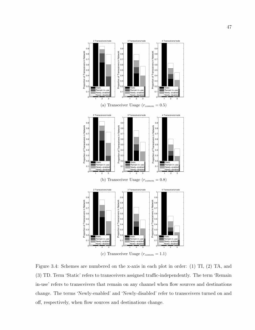
47

1 2 30

0.1

0.2

0.3

0.4

0.5

0.6

0.7

0.8

0.9

12 Transceivers/node

Pro

po

rtio

n o

f T

ran

sce

ive

rs in

Ne

two

rk

Static

Remain in−use

Newly−enabled

Newly−disabled

1 2 30

0.1

0.2

0.3

0.4

0.5

0.6

0.7

0.8

0.9


Pro

po

rtio

n o

f T

ran

sce

ive

rs in

Ne

two

rk

Static

Remain in−use

Newly−enabled

Newly−disabled

1 2 30

0.1

0.2

0.3

0.4

0.5

0.6

0.7

0.8

0.9


Pro

po

rtio

n o

f T

ran

sce

ive

rs in

Ne

two

rk

Static

Remain in−use

Newly−enabled

Newly−disabled

(a) Transceiver Usage (rcomm = 0.5)

1 2 30

0.1

0.2

0.3

0.4

0.5

0.6

0.7

0.8

0.9


Pro

po

rtio

n o

f T

ran

sce

ive

rs in

Ne

two

rk

Static

Remain in−use

Newly−enabled

Newly−disabled

1 2 30

0.1

0.2

0.3

0.4

0.5

0.6

0.7

0.8

0.9


Pro

po

rtio

n o

f T

ran

sce

ive

rs in

Ne

two

rk

Static

Remain in−use

Newly−enabled

Newly−disabled

1 2 30

0.1

0.2

0.3

0.4

0.5

0.6

0.7

0.8

0.9


Pro

po

rtio

n o

f T

ran

sce

ive

rs in

Ne

two

rk

Static

Remain in−use

Newly−enabled

Newly−disabled

(b) Transceiver Usage (rcomm = 0.8)

1 2 30

0.1

0.2

0.3

0.4

0.5

0.6

0.7

0.8

0.9


Pro

port

ion o

f T

ransceiv

ers

in N

etw

ork

Static

Remain in−use

Newly−enabled

Newly−disabled

1 2 30

0.1

0.2

0.3

0.4

0.5

0.6

0.7

0.8

0.9


Pro

port

ion o

f T

ransceiv

ers

in N

etw

ork

Static

Remain in−use

Newly−enabled

Newly−disabled

1 2 30

0.1

0.2

0.3

0.4

0.5

0.6

0.7

0.8

0.9


Pro

port

ion o

f T

ransceiv

ers

in N

etw

ork

Static

Remain in−use

Newly−enabled

Newly−disabled

(c) Transceiver Usage (rcomm = 1.1)

Figure 3.4: Schemes are numbered on the x-axis in each plot in order: (1) TI, (2) TA, and

(3) TD. Term ‘Static’ refers to transceivers assigned traffic-independently. The term ‘Remain

in-use’ refers to transceivers that remain on any channel when flow sources and destinations

change. The terms ‘Newly-enabled’ and ‘Newly-disabled’ refer to transceivers turned on and

off, respectively, when flow sources and destinations change.

48

when rcomm = 1.1, the network supports 18% higher flow rate. This is due to needing more

resources on average to serve traffic over more hops.

In addition to achieving a higher flow rate, the TA scheme uses fewer transceivers, an energy-

saving bonus. As compared to the TI scheme, it enables 13%, 36%, and 50% fewer transceivers

when nodes are equipped with 2, 3, and 4 transceivers, respectively, on average across all

scenarios. We track how the TA scheme and the TD scheme adapt their assignments to

achieve their respective maximum flow rates.

There are 36%, 42%, and 43% fewer transceivers used in the TD scheme than in the TA

scheme in the 2-, 3-, and 4-transceiver scenarios, respectively, when averaged across all values

of rcomm. This is due to the connectivity requirements we place on the TA scheme.

However, the TD scheme has 154%, 46%, and 36% more transceivers that are newly-enabled

in the 2-, 3-, and 4- transceiver scenarios, respectively, averaged across all values of rcomm, and

the TD scheme has 156%, 57%, and 50% more newly-disabled transceivers on average. This

represents more fluctuations in the topology. In practice, such fluctuations induce control

traffic at multiple layers, which takes away from network goodput and leaves the network

vulnerable to control traffic storms.

When evaluating the resource allocation patterns with different values of rcomm, the propor-

tion of transceivers used in the TA and TD schemes decreases as rcomm increases. This is

because fewer resources are necessary to service each flow on average when hop count for

each, which is an effect of increasing rcomm. When focusing on the TA scheme’s transceiver

allocation patterns in isolation, the TA scheme allocates slightly fewer transceivers indepen-

dently of traffic conditions as rcomm increases. This is because each node can reach more of

its neighbors when rcomm is higher, requiring fewer multi-hop paths and fewer transceiver-

channel assignments to preserve the aggregate interference constraint.

49

0 0.1 0.2 0.3 0.4 0.5 0.6 0.7 0.8 0.9 10

0.5

1

1.5

2

2.5

3

α vs. k’−connectivity

Proportion of Transceivers Allocated Independently of Traffic Conditions (α)

k’−

connectivity

2 Transceivers/node

3 Transceivers/node

4 Transceivers/node

(a) α versus k′-connectivity

0 0.1 0.2 0.3 0.4 0.5 0.6 0.7 0.8 0.9 10

0.2

0.4

0.6

0.8

1

1.2

α vs. Flow Rate


Ma

xim

um

Flo

w R

ate

2 Transceivers/node

3 Transceivers/node

4 Transceivers/node

(b) α versus Flow Rate

Figure 3.5: Relationships among α, k′, and r with rcomm = 0.5

3.2.3 Effects of Variable α

We have shown the benefits of the the TA allocation as compared to a completely TI approach

(α = 1) and a completely TD approach (α = 0), but there is a tradeoff space where the

proportion of resources allocated traffic-independently, α, can fall between 0 and 1. Note

that 1 − α is the proportion of resources available to be allocated in response to traffic

demand. As α grows, fewer resources are available to adapt the network to changing traffic

demand. At the other end of the spectrum, if α is too low, the network may not have

sufficient baseline connectivity.

In this scenario, the parameters are the same as in the previous subsection. Figures 3.5a,

3.6a, 3.7a show the relationship between the proportion of resources allocated independently

of traffic conditions (α) and the average k′-connectivity. We expect a monotonic increase in

k′-connectivity as α increases, but we note the importance of how k′ increases from α = 0

to α = 1. For each scenario, there is a slow growth rate in k′ initially with respect to α.

Then, the slope of k′ increases for values of α that correspond to a k′-connectivity in the

50

0 0.1 0.2 0.3 0.4 0.5 0.6 0.7 0.8 0.9 10

1

2

3

4

5

6



k’−

connectivity

2 Transceivers/node

3 Transceivers/node

4 Transceivers/node


0 0.1 0.2 0.3 0.4 0.5 0.6 0.7 0.8 0.9 10

0.2

0.4

0.6

0.8

1

1.2

1.4

1.6

α vs. Flow Rate


Maxim

um

Flo

w R

ate

2 Transceivers/node

3 Transceivers/node

4 Transceivers/node



0 0.1 0.2 0.3 0.4 0.5 0.6 0.7 0.8 0.9 10

1

2

3

4

5

6

7

8

9



k’−

connectivity

2 Transceivers/node

3 Transceivers/node

4 Transceivers/node


0 0.1 0.2 0.3 0.4 0.5 0.6 0.7 0.8 0.9 10

0.5

1

1.5

2

α vs. Flow Rate


Ma

xim

um

Flo

w R

ate

2 Transceivers/node

3 Transceivers/node

4 Transceivers/node



51

range of k′ = (0.5, 2.0), indicating that there is a larger payoff in terms of connectivity for

the resources allocated in this region. For larger values of α (k′ > 2, k′ > 3, k′ > 7 for

scenarios of rcomm = 0.5, rcomm = 0.8, and rcomm = 1.1 respectively), the curve flattens,

indicating that additional TI allocation of resources brings about diminishing payoff in terms

of k′-connectivity. Although the point of diminishing return, in terms of maximizing k′, is

higher in the scenario with rcomm = 1.1, there are practical considerations to stop allocating

additional resources when the topology has achieved sufficiently high connectivity (i.e. Is it

necessary to allocate more resources to reach a k-connectivity of 7 if the topology is already

6-connected?).

Figures 3.5b, 3.6b, and 3.7b shows the proportion of TI resources allocated, α, versus flow

rate. We expect to see a monotonic decrease in flow rate as α increases because as α increases,

the flexibility of the network’s channel assignment decreases, meaning its dynamic response

to traffic demand will have more limited effectiveness.

For low levels of α the flow rate does not decrease any as α grows, and all scenarios (at a

common value of rcomm) are roughly equivalent with respect to flow rate. The flow rate in the

scenario with 2 transceivers per node drops off more quickly than in the scenarios with 3 and

4 transceivers per node. In each scenario, the rate of decrease in flow rate accelerates as α

increases. The results show a flow-rate plateau (especially for 3 and 4 transceivers per node),

and to the right of the plateau the descent is steepest in scenarios with more transceivers per

node. As α approaches 1, the gap between all flow rates narrows. This was found to also be

true at α = 0, indicating that there is less flow-rate benefit associated with increasing the

number of radios at α = 0 or α = 1 as compared to other values of α. This further weakens

the justifications for using a strictly TI or TD scheme in networks.

52

3.3 Conclusion

In this chapter, we introduce a new approach to channel assignment in the context of multi-

hop, multi-channel, multi-radio wireless networks and, more broadly, cognitive networks and

dynamic spectrum access networks. We outline a traffic-aware (TA) approach to channel

assignment. The TA approach has two stages of channel assignment in which the first stage

is a resource-minimized traffic-independent (TI) assignment and the second stage is a traffic-

driven (TD) assignment. The TI assignment provides basic network connectivity with limited

interference, enabling light traffic demands and basic network maintenance functions (e.g.

serving control traffic). By allocating a minimum number of transceivers or radios for the

TI component, resources are conserved as much as possible for the TD component, which is

influenced by traffic demand. The conserved radios are dynamically assigned in response to

traffic stimuli to maximize flow rate. As traffic conditions change, the TD assignments are

re-optimized for current traffic conditions while the TI component remains unchanged.

Overall, results indicate that our TA scheme:

1. supports higher flow rate than a strictly TI scheme while using fewer radios,

2. approaches the flow rate of a strictly TD scheme in the 3- and 4-transceiver scenarios

explored, and

3. has fewer fluctuations in channel allocations than a strictly TD allocation.

By finely varying the proportion of resources allocated independently of traffic conditions

(α), we saw that k′-connectivity (a metric we define which is closely related to traditional

k-connectivity) monotonically increases as a function α. Beyond a certain point, there are

diminishing returns in terms of additional network connectivity gained through the allocation

of additional radios for connectivity. Also, we see that flow rate r decreases as a function of

53

α, and beyond a certain point the average flow rate diminishes more quickly. Both of these

observations suggest adopting a resource-minimized, traffic-independent channel assignment

in order to keep α as low as possible while still maintaining network connectivity.

In Chapter 4, we present a set of heuristic algorithms that address the resource-minimization

problem, RM, and effectively approximate RM. We analyze how effective the algorithms

are at minimizing resources in the TI allocation with respect to the optimal approach (RM)

and other related approaches in the research literature. In Chapter 5, we focus on how

to allocate resources in response to traffic conditions in a distributed fashion taking into

consideration additional dynamics of traffic conditions, namely imbalanced flow demands.

Chapter 4

Traffic-independent Channel

Assignment

In Chapter 3, we outlined the benefits of a traffic-aware (TA) approach as compared to

traffic-independent (TI) and traffic-driven (TD) approaches. The TA approach is a two-stage

approach that assigns some transceivers (to channels) independently of traffic conditions in

the first stage and some transceivers in response to traffic conditions in the second stage.

In Chapter 3, we evaluated the soundness of the TA approach with a set of mixed-integer

linear programs (MILPs), and we found that the TA approach exhibits the benefits of both

completely TI and TD approaches without any major drawbacks.

In this chapter, we focus on the first stage of the TA approach: the resource-minimized TI

stage. The goal of the resource-minimized TI stage is to assign as few transceivers as possible

to achieve a baseline network connectivity. The motivation for a resource-minimized, TI

allocation is to save energy by enabling as few transceivers as possible. Also, by conserving

resources in the TI stage, the network has a higher maximum achievable flow rate because

there is greater flexibility in the network’s channel assignment in the TD stage, as was shown

in Chapter 3.

54

55

In this chapter, we review the TA, two-stage MILP from Chapter 3. We present centralized

and distributed greedy heuristic schemes that minimize resource allocation in the TI stage.

We compare these schemes to the optimum and to other schemes from the research literature.

We compare several statistics on the resulting traffic-independent topology, including the

number of transceiver assignments, network graph connectivity, and conflict degree. We also

compare all schemes in terms of the maximum achievable flow rate. Since our focus is on the

TI assignment, we fix the second (TD) stage assignment to follow an optimal TD MILP1.

The contributions of this chapter include comparing an optimal resource-minimized TI scheme,

which is formulated in Section 4.1 (which is the identical to the formulation from Subsec-

tion 3.1.1), to two greedy heuristic approaches. The centralized approach, called centralized

resource-minimized channel assignment (RMCA), is presented in Section 4.2, while the dis-

tributed approach, called distributed RMCA, is presented in Section 4.3. We present the

numerical procedure and results in Section 4.4.

4.1 Problem Formulation

In this section, we provide the two-stage MILP formulation of TA channel assignment that

was first provided in Chapter 3. Figure 3.1 from Chapter 3 shows the basic idea of the ap-

proach. The first (TI) stage assigns channels, inducing a topology that does not change based

on traffic conditions. The second (TD) stage assigns channels to any unused transceivers from

the first stage, based on traffic conditions, with the goal of maximizing throughput by mod-

ifying the topology to be more suited to the current traffic demand. Under changing traffic

conditions, the topology can be re-optimized to meet the current traffic demands.

The first (TI) stage assigns channels independently of traffic conditions to establish connec-

tivity. The objective is to assign as few transceivers (to channels) as possible throughout the

1Traffic-driven assignment is the subject of Chapter 5.

56

network such that a connected, multi-channel topology is established with limited interfer-

ence. We denote this as problem RM.

The first stage of the TA problem formulation is problem RM. See Subsection 3.1.1 for the

details of the formulation. Problem RM reads as follows.

min∑i∈V

|Ci|

subject to

|Ci| ≤ T (∀i ∈ V)

|Pij| ≥ 1 (∀i ∈ V ,∀j ∈ V)∑j∈V,j 6=i

(IR[i][j]− CR[i][j]) · |Cij| = 0 (∀i ∈ V)

The second stage of the TA problem formulation is problem FM. This problem assigns any

unused transceivers from problem RM to maximize end-to-end flow rate. Problem FM

reads as follows.

57

max∑f∈F

wf · r

subject to

|Ci| ≤ T (∀i ∈ V)∑j∈V,j 6=i

lij(c) +∑

j∈V,j 6=i

lji(c) ≤ γ (∀i ∈ V , c ∈ Ci)

∑j∈V

∑k∈V,k 6=j

ljk(c) · IR[j][i] ≤ γ (∀i ∈ V ,∀c ∈ Ci)

∑f∈F


lij(c) · CR[i][j] (∀i ∈ V ,∀j ∈ V , j 6= i)

∑j∈V,j 6=i

tij(f) =∑

k∈N ,k 6=i

tki(f) (∀f ∈ F ,∀i ∈ V ,

i 6= s(f), d(f))

∑j∈V,j 6=i

tij(f) = r (∀f ∈ F , i = s(f))

tij(f) ≥ 0 (∀i ∈ V ,∀j ∈ V ,

∀f ∈ F)

lij(c) ≥ 0 (∀i ∈ V ,∀j ∈ V ,

∀c ∈ C)

58

4.2 Centralized RMCA

The running time necessary to solve problem RM (the optimal TI channel assignment)

grows exponentially with the dimension of the problem’s parameters (|V|, T , and |C|). In

this section, we present a centralized heuristic approach, in which the running time grows in

polynomial time with the problem’s parameters. The goal of this approach, which we denote

as centralized RMCA, is the same in that it addresses the problem of resource-minimized,

traffic-independent channel assignment with the objective of assigning as few transceivers in

the network as possible such that the network is connected and has limited interference.

4.2.1 The Centralized RMCA Algorithm

We outline the algorithm in this subsection and provide pseudocode in Algorithm 1. We

utilize the higher granularity of the k′-connectivity metric (as compared to traditional k-

node-connectivity) to guide the channel assignment to reach a graph connectivity of k ≥ 1

using as few channels as possible. See Subsection 3.1.2 for the definition of this metric.

Starting with an empty channel assignment at all nodes, the basic idea of this approach is

to iteratively assign channels to node transceivers, with each assignment yielding the highest

possible increase in the graph’s k′-connectivity (∆k′). Essentially, we greedily maximize k′

with each assignment, and there is an intelligent process for handling the situation where

no increase in k′ is possible. Since the objective is to connect the network using as few

transceivers as possible, the algorithm terminates once k ≥ 1 (or an equivalent stop condition

is k′ ≥ 1). Although we focus on reaching k ≥ 1, the algorithm can be easily extended to

target greater values of k or k′.

First, we score the potential assignment of each channel at each node, with the score being the

change in the graph’s k′-connectivity (∆k′) due to the assignment if the channel is eligible. At

59

node i ∈ V , the channel eligibility set Cei is defined as C\{Ci∪⋃j∈IRi\CRi

Cj}. This results in

a |V| x |C| matrix of scores. A negative score, indicating an ineligible assignment, is given to

all channels at a node if the node has no free transceivers, and a negative score is given for any

channel at nodes which introduce any interference, which enforces the interference constraint.

Also, if the node is already assigned a particular channel a negative score is given, preventing

subsequent assignment of the same channel. Second, if the maximum node-channel score is

greater than zero, the channel assignment corresponding to the entry is performed with any

ties broken by selecting the lowest indexed node and channel. The process repeats starting

with another scoring of the channels.

Oftentimes, the maximum score will equal zero (e.g. the first assignment in the network),

so we provide the following procedure for assigning a channel when this is the case. First,

two conditions are tested sequentially. If both conditions are false, there is a default assign-

ment. Note that if all scores are negative, no channel assignment occurs and the algorithm

terminates (since no channel assignment is eligible).

Condition 1: There exists a node i ∈ V that has a degree equal to 0 and |Cei | > 0. If the

condition is true the lowest-indexed eligible channel is assigned at the node of degree 0. If

multiple nodes have a degree of 0, select the lowest-indexed node. The point is that we are

trying to go from a k-connectivity of 0 to 1. Since k is bounded by the minimum node degree

in the network graph, denoted δ(G), we must ensure that every node has degree of at least 1

before we can achieve a connectivity of 1.

Condition 2: There exists a source-destination node-pairing (i, j) such that PNDij is equal

to 0 and |Cei | + |Cej | > 0 (either i or j has an eligible channel). If the condition is true, we

assign an eligible channel to either node i or j. If both have an eligible channel, we select the

node with the lower node degree: argmin(|Ei|, |Ej|), where Ei is the set of edges at node i. If

nodes i and j have equal node degree and at least one eligible channel, we select the node

with the lower index. The motivation is that in order for the network to reach a connectivity

60

of 1 all node pairings (i, j) must have PNDij ≥ 1, so we attempt to increase any PND

ij that is

equal to 0.

Default: If conditions (1) and (2) are false, we select the node with the least number of

channels assigned and an eligible channel to assign and assign that node an eligible channel.

As before, all ties are broken by choosing the lowest indexed channel or node index.

4.2.2 Centralized RMCA Running Time

To analyze the running time of the centralized RMCA algorithm, we recognize that the overall

running time is heavily dependent on the implementation of line number 6, which computes

the graph’s change in k′-connectivity. First, we discuss the running time of computing this

metric, and then we show how it affects the overall running time of the algorithm.

In order to compute the graph’s k′-connectivity, we need to find the number of node-disjoint

paths |PNDij | for all i, j ∈ V node-pairings. For a single node-pairing, we solve the traditional

max-flow problem from one node to the other using a built-in MATLAB function called

‘graphmaxflow’ [48]. Since the function solves the problem on the set of edges in the network

graph, we use an expander-graph transformation2. The function ‘graphmaxflow’ uses the

Goldberg algorithm [48] which has complexity O(|V|2 ·√|E|) [49]. Note that the graph

transformation only affects the running time by a constant factor. Since we solve the max-flow

problem for all node-pairings, the running time of computing k′-connectivity is O(|V|4 ·√|E|).

The loops surrounding line 6 further increase the running time of the centralized RMCA

algorithm. The algorithm’s outer loop is a ’while’ loop that will run at most V ·T times. The

loops on line 3 and 4 iterate through each node-channel combination. Overall, the running

time of the centralized RMCA algorithm is O(T · |C| · |V|6 ·√|E|).

2In the adopted expander-graph transformation, undirected edges are transformed into two directed edges

and each node represents two nodes in the transformed graph. The first node is an endpoint for all incoming

edges of the original node and has a single directed edge to the second node. The second node is an endpoint

of all outgoing edges.

61

Algorithm 1 Centralized RMCA Algorithm

1: Ci ← ∅,∀i ∈ V

2: while k < 1 do

3: for all i ∈ V do

4: for all c ∈ C do

5: if Ci∪{c} is eligible then

6: score[i][c] ← ∆k′ of G with Ci∪{c}

7: else

8: score[i][c] ← −1

9: end if

10: end for

11: end for

12: (i∗, c∗)← argmaxi∈V,c∈C(score[i][c])

13: if score[i∗][c∗] > 0 then

14: Ci∗ ← Ci∗∪{c∗}

15: else if score[i∗][c∗] = 0 then

16: if Condition 1 is true then

17: i∗ ← argminı∈V(δ(G)) : |Cei∗| > 0

18: c∗ ← argmaxc∈C(score[i∗][c])

19: else if Condition 2 is true then

20: (i∗, j∗)← argmini∈V,j∈V\i(PNDij ))

21: if (|Ej∗| < |Ei∗| and |Cej∗| > 0) or (Cei∗ = ∅) then

22: i∗ ← j∗

23: end if


25: else

26: i∗ ← argmini∈V(|Ci|) : |Cei∗| > 0


62

28: end if

29: Ci∗ ← Ci∗∪{c∗}

30: else

31: Terminate, no channel assignment is eligible

32: end if

33: end while

4.3 Distributed RMCA

In this section, we present a distributed scheme to the problem of resource-minimized, traffic-

independent channel assignment, which is adapted from our prior work in [10]. A distributed

channel assignment algorithm may be necessary when centralized control is not possible (e.g.

in ad hoc networks).

4.3.1 Assumptions

Each node uses local information to assign channels. We assume that through some local

neighbor discovery process nodes are aware of all other nodes within reliable communication

range, which at node i is denoted as set CRi. Also, through some channel sensing mechanism,

we assume that nodes can sense interference on a channel, which is defined as the presence

of another node on a channel where the other node is outside of communication range but

within interference range.

Any two nodes that are within communication range of each other and have at least one

channel in common are neighbors. The set of neighbors at node i is defined as Ni ={j ∈ CRi

| Cij 6= ∅}. We assume that neighboring nodes can become aware of each other’s 1-hop

neighbors, making nodes aware of all 2-hop neighbors. This is possible through standard

control messages (e.g. HELLO messages). The set of all nodes in the 2-hop neighborhood of

node i is defined as N 2i ={k ∈ Nj | j ∈ Ni, k 6= i}.

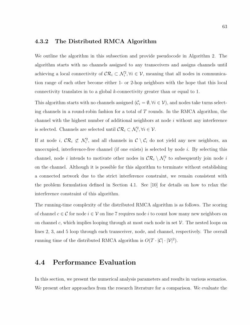
63

4.3.2 The Distributed RMCA Algorithm

We outline the algorithm in this subsection and provide pseudocode in Algorithm 2. The

algorithm starts with no channels assigned to any transceivers and assigns channels until

achieving a local connectivity of CRi ⊂ N 2i ,∀i ∈ V , meaning that all nodes in communica-

tion range of each other become either 1- or 2-hop neighbors with the hope that this local

connectivity translates in to a global k-connectivity greater than or equal to 1.

This algorithm starts with no channels assigned (Ci = ∅,∀i ∈ V), and nodes take turns select-

ing channels in a round-robin fashion for a total of T rounds. In the RMCA algorithm, the

channel with the highest number of additional neighbors at node i without any interference

is selected. Channels are selected until CRi ⊂ N 2i ,∀i ∈ V .

If at node i, CRi 6⊂ N 2i , and all channels in C \ Ci do not yield any new neighbors, an

unoccupied, interference-free channel (if one exists) is selected by node i. By selecting this

channel, node i intends to motivate other nodes in CRi \ N 2i to subsequently join node i

on the channel. Although it is possible for this algorithm to terminate without establishing

a connected network due to the strict interference constraint, we remain consistent with

the problem formulation defined in Section 4.1. See [10] for details on how to relax the

interference constraint of this algorithm.

The running-time complexity of the distributed RMCA algorithm is as follows. The scoring

of channel c ∈ C for node i ∈ V on line 7 requires node i to count how many new neighbors on

on channel c, which implies looping through at most each node in set V . The nested loops on

lines 2, 3, and 5 loop through each transceiver, node, and channel, respectively. The overall

running time of the distributed RMCA algorithm is O(T · |C| · |V|2).

4.4 Performance Evaluation

In this section, we present the numerical analysis parameters and results in various scenarios.

We present other approaches from the research literature for a comparison. We evaluate the

64

Algorithm 2 Distributed RMCA Algorithm

1: Ci ← ∅,∀i ∈ V

2: for t = 1 to T do

3: for i ∈ V do

4: if CRi 6⊂ N 2i then

5: for c ∈ C do

6: if no interference sensed on channel c then

7: score[c] ← |{j ∈ CRi \ N 2i | c ∈ Cj}|

8: else

9: score[c] ← −1

10: end if

11: end for

12: c∗ ← argmaxc∈C(score[c])

13: if score[c∗] ≥ 0 then

14: Ci ← Ci∪{c∗}

15: end if

16: end if

17: end for

18: end for

65

characteristics of the traffic-independent topology generated. Subsequently, we show how the

traffic-independent topology affects the network’s ability to dynamically respond to changing

traffic conditions.

4.4.1 Algorithms

Prior to discussing the numerical procedure, we outline the most relevant approaches from

the research literature and how they are used in our evaluation. In [18], an approach called

Interference-Aware Topology Control (IA-TC) is proposed. In the first step of IA-TC, the

authors propose a topology control scheme called Minimal Interference Survivable Topology

Control (INSTC) that selects a threshold of minimal conflict weight where the set of edges

below the threshold connect the graph and will subsequently be assigned channels. In de-

creasing order of conflict weight, the edges are greedily assigned the least used channels in

interference range. Depending on the problem parameters, some nodes may have unassigned

transceivers. In [18], these unassigned transceivers are assigned the least used channel in the

node’s interference range in the last step; however, we adapt this last step by assigning any

unassigned transceivers in response to traffic conditions to more fairly compare the work in

[18] to our work.

In [19], a channel assignment algorithm titled Connected Low Interference Channel Assign-

ment (CLICA) is proposed. The algorithm takes as input a graph (with edges assigned

channels). Similar to IA-TC the edges are assigned channels that are in minimal use within

interference range; however, the order in which edges are assigned adapts based on how many

transceivers remain at each node. The nodes with only a single unassigned transceiver are

given the highest priority to be assigned next. The resulting channel assignment assigns

channels to all edges and may leave nodes with unassigned transceivers. In our performance

analysis, we denote two algorithms following the approach of CLICA with different input

graphs. The first approach, denoted CLICA, takes as input the colorless communication

66

graph with edges existing between nodes that are within communication range of each other.

The second approach, denoted INSTC-CLICA, takes as input the subgraph of the colorless

communication graph following the INSTC procedure. Refer to [18] for details on IA-TC

and INSTC and to [19] for details on CLICA.

In [12], the authors propose the formation of maximal cliques or frequency clusters where

nodes within communication range of one another congregate on a common channel. The

benefit of a topology of cliques is increased medium access control (MAC) efficiency from

eliminating hidden terminals. In this approach, nodes start with no initial channel assignment

and sequentially select channels. During channel selection, a node will choose to join the

largest clique possible. To join the clique, a node must be within communication range of all

other nodes within the clique. If there are no available cliques, then a node selects an unused

channel (unused within its interference range disk) in order to attract other surrounding

nodes to join the node on that channel to form a clique. In this process, all transceivers are

assigned if there is a sufficient number of channels. In this approach, there are no transceivers

assigned in response to traffic conditions, and it will be shown that this lack of traffic-driven

assignment yields lower flow throughput.

Another related approach for addressing TI connectivity is to dedicate a transceiver to a

network-wide control channel. This approach is analyzed in different scenarios in [35–37, 42,

44]. To evaluate the control channel approach against the TA scheme, we assign a single

transceiver of every node to the lowest-indexed channel in the TI stage. Although this

approach represents the absolute minimum number of transceivers allocated, there are many

pitfalls with such an approach (e.g. control channel congestion or the possibility of hidden

terminals). We quantify this in our numerical results.

4.4.2 Numerical Results

The numerical procedure follows the approach presented in Figure 3.1, where the TI assign-

ment forms a connected topology in the first stage, and in the second stage the topology

67

adapts to maximize flow rate. We vary the approaches to channel assignment in the first

stage, and the second stage is the solution of problem FM, as presented in Section 4.1, using

any unassigned transceivers from the first stage.

We run multiple simulations to characterize the flow rates using each approach. We set the

number of nodes, |V|, to 20. Nodes are placed in a rectangular area with edges of length

2 and 0.5, and we vary rcomm, effectively varying node density, to be 0.5, 0.8, and 1.1 with

rint = 1.75·rcomm. The variation in communication range causes the network diameter to vary

from 2 to 6 hops. Using a rectangle, as opposed to a square, allows us to see 6-hop network

diameters without increasing the number of nodes too much. We also vary the number of

transceivers per node from 2 to 4.

In Figures 4.1 - 4.3, we count the number of transceivers assigned independently of traffic

conditions. We see that the centralized RMCA algorithm performs near identically to the

optimal approach (the solution to problem RM) in the scenarios evaluated. The distributed

RMCA algorithm assigns slightly more transceivers than does the optimal approach, but it

assigns as little as one third fewer transceivers than the other approaches. Also, as rcomm

increases, the distributed RMCA algorithm performs close to optimal. Averaging all the

scenarios together, the distributed RMCA algorithm performed within 9% of the optimal

approach. As the number of transceivers per node increases, the gap between the other ap-

proaches and the optimal grows. However, this is not true for the centralized and distributed

RMCA algorithms. Reducing the number of transceivers allocated independently of traffic

conditions reduces the energy consumption since there is a non-negligible cost in enabling

and operating a transceiver.

Figures 4.4 - 4.6 show the k′-connectivity of each TI allocation scheme. We see that the TA

approach successfully achieves at least a 1-connected network in all scenarios 3 Moreover, the

3Although each scenario has a uniformly random placement of nodes in a rectangular area, we filter out

the random placements where nodes are located such that the communication range is not large enough to

produce a connected network (i.e., the smallest gap between a node and all the other nodes is greater than

distance rcomm).

68

0.5 0.8 1.10

0.1

0.2

0.3

0.4

0.5

0.6

0.7

0.8

0.9

1Assignment (T = 2)

rcomm

Pro

port

ion o

f T

ranscie

vers

enable

d (

TI)

Optimal RMCA

Central. RMCA

Distr. RMCA

CLICA

IA−TC

CLICA−INSTC

Maximum Clique

Control Channel

Figure 4.1: Proportion of Network Transceivers Assigned (T = 2)

0.5 0.8 1.10

0.1

0.2

0.3

0.4

0.5

0.6

0.7

0.8

0.9

1Assignment (T = 3)

rcomm

Pro

po

rtio

n o

f T

ran

scie

ve

rs e

na

ble

d (

TI)

Optimal RMCA

Central. RMCA

Distr. RMCA

CLICA

IA−TC

CLICA−INSTC

Maximum Clique

Control Channel


69

0.5 0.8 1.10

0.1

0.2

0.3

0.4

0.5

0.6

0.7

0.8

0.9

1Assignment (T = 4)

rcomm

Pro

po

rtio

n o

f T

ran

scie

ve

rs e

na

ble

d (

TI)

Optimal RMCA

Central. RMCA

Distr. RMCA

CLICA

IA−TC

CLICA−INSTC

Maximum Clique

Control Channel


other schemes tend to approach much higher levels of k′-connectivity, which we argue may

be unnecessary for a TI allocation scheme.

Having high graph connectivity typically implies that nodes must time-multiplex the channels

they are on more in order to avoid collisions. To quantify this, we define the conflict degree

at node i, δi, as the number of nodes within distance rcomm of node i tuned to a common

channel of i: δCi = |j ∈ IRi : Cij 6= ∅|.

Figures 4.7 - 4.9 show the average conflict degree of each approach. The importance of the

conflict degree of the TI topology is that the TI allocation is dedicated to supporting light

demands of network control traffic. Assuming each node broadcasts4 control traffic to all

other nodes on their common channels, the maximum amount of control traffic supported

is inversely proportional to the conflict degree. The lower the conflict degree the less time-

sharing of the channel is necessary to avoid collisions of control traffic.

In addition to saving energy and exhibiting a lower conflict degree, in Figures 4.10 - 4.12, the

RMCA algorithms greatly outperform the approaches from the research literature in terms of

4Here broadcast refers to a MAC layer broadcast message like a HELLO message.

70

0.5 0.8 1.10

2

4

6

8

10

12k’−connectivity (T = 2)

rcomm

k’−

connectivity

Optimal RMCA

Central. RMCA

Distr. RMCA

CLICA

IA−TC

CLICA−INSTC

Maximum Clique

Control Channel

Figure 4.4: k′-connectivity (T = 2)

0.5 0.8 1.10

2

4

6

8

10


rcomm

k’−

connectivity

Optimal RMCA

Central. RMCA

Distr. RMCA

CLICA

IA−TC

CLICA−INSTC

Maximum Clique

Control Channel


71

0.5 0.8 1.10

2

4

6

8

10


rcomm

k’−

connectivity

Optimal RMCA

Central. RMCA

Distr. RMCA

CLICA

IA−TC

CLICA−INSTC

Maximum Clique

Control Channel


0.5 0.8 1.10

2

4

6

8

10

12

14

16

18

20Average Conflict Degree (T = 2)

rcomm

Co

nflic

t D

eg

ree

Optimal RMCA

Central. RMCA

Distr. RMCA

CLICA

IA−TC

CLICA−INSTC

Maximum Clique

Control Channel

Figure 4.7: Average Conflict Degree per Node (T = 2)

72

0.5 0.8 1.10

2

4

6

8

10

12

14

16

18


rcomm

Conflic

t D

egre

e

Optimal RMCA

Central. RMCA

Distr. RMCA

CLICA

IA−TC

CLICA−INSTC

Maximum Clique

Control Channel


0.5 0.8 1.10

2

4

6

8

10

12

14

16

18


rcomm

Co

nflic

t D

eg

ree

Optimal RMCA

Central. RMCA

Distr. RMCA

CLICA

IA−TC

CLICA−INSTC

Maximum Clique

Control Channel


73

flow rate in almost all of the scenarios evaluated. Given that the centralized RMCA algorithm

nearly matches the optimal approach in the number of transceivers assigned, we expect the

flow rate to also nearly match the optimal since the centralized RMCA approach because it

conserves about as much resources for TD adaptation as does the optimal approach.

Although the distributed RMCA algorithm achieves within 9% of the optimum in terms of the

number of transceivers assigned independently of traffic conditions, it achieves within 3.5% of

the optimum in terms of maximum achievable flow rate averaged over all evaluated scenarios.

The slight sub-optimality of the distributed RMCA algorithm in terms of the number of

traffic-independently assigned transceivers only slightly hinders the maximum achievable flow

rate because there are enough transceivers conserved to address traffic demands.

In the scenarios with rcomm = 0.5, the difference between the optimal flow rate and the other

approaches is smaller, especially in the scenario with four transceivers per node. When rcomm

is low, nodes are effectively more spread out and the number of possible communication links

is less than when rcomm is higher, so there are fewer possible adaptations, leading to less

improvement with a TD channel assignment. In the scenario with four transceivers per node,

the TI assignment of the other schemes assigns channels to many of the possible communi-

cation links over multiple channels, leaving less possibility for adaptation to maximize flow

rate with a TD assignment.

Although the maximum achievable flow rates are similar in the scenario with rcomm = 0.5

and four transceivers per node, the cost is shown in Figure 4.3 where other schemes allocate

almost three times the number of transceivers in the TI stage of channel assignment. The

higher the number of TI transceivers, the higher the cost is in terms of energy consumption

and, potentially, network lifetime.

74

0.5 0.8 1.10

0.2

0.4

0.6

0.8

1

1.2

1.4Flow Rate (T = 2)

rcomm

Flo

w R

ate

Optimal RMCA

Central. RMCA

Distr. RMCA

CLICA

IA−TC

CLICA−INSTC

Maximum Clique

Control Channel

Figure 4.10: Flow Rate (2 Transceivers per Node)

0.5 0.8 1.10

0.5

1

1.5

2


rcomm

Flo

w R

ate

Optimal RMCA

Central. RMCA

Distr. RMCA

CLICA

IA−TC

CLICA−INSTC

Maximum Clique

Control Channel


75

0.5 0.8 1.10

0.5

1

1.5

2


rcomm

Flo

w R

ate

Optimal RMCA

Central. RMCA

Distr. RMCA

CLICA

IA−TC

CLICA−INSTC

Maximum Clique

Control Channel


4.5 Conclusion

The central motivation for this dissertation is to find an effective strategy for channel as-

signment in a cognitive radio network in which nodes have multiple transceivers. Such a

channel assignment scheme should achieve connectivity, exhibit minimal interference, and

be adaptive to the network’s dynamic traffic demands. We show a two-stage traffic-aware

approach to channel assignment that has these characteristics.

In this chapter, we focus on the first stage of the TA approach: the traffic-independent stage.

We formulate an optimal approach with problem RM, which follows an MILP and finds the

minimum number of transceiver assignments in the network such that the network is con-

nected and has limited interference. We develop two heuristic algorithms called centralized

RMCA and distributed RMCA. We find that our proposed approaches perform much closer

to optimal than other proposed approaches in the research literature in terms of the number

of transceiver-channel assignments necessary to maintain network connectivity. Also, the

resource-minimized approaches achieve a more appropriate level of connectivity than other

approaches, resulting in a lower conflict degree.

76

In order to evaluate the impact of the TI assignment on the maximum achievable flow rate,

we formulate flow maximization problem FM, which follows an MILP of channel assignment

(of transceivers not dedicated traffic-independently to maintaining network connectivity) and

flow routing. To fairly compare each TI scheme’s impact on flow rate, problem FM is solved

to assign any transceivers not assigned traffic-independently to maximize flow rate. We find

that the resource-minimized approaches are able to achieve a higher maximum flow rate than

other approaches due to using fewer transceivers for TI channel assignment. Furthermore,

our approaches achieve within 3.5% of the optimal (the solutions of both RM and FM)

flow rate averaged across all evaluated scenarios.

This chapter advances the main idea of the dissertation, a traffic-aware approach to channel

assignment, and provides a set of approaches for traffic-independent channel assignment.

In Chapter 5, we focus on the second stage of the TA approach of traffic-driven channel

assignment, and we illustrate how the TA approach performs in an event-driven simulation

with a more realistic traffic model.

Chapter 5

Traffic-driven Channel Assignment

In Chapter 3, we outlined the basic idea of a traffic-aware (TA) approach to channel assign-

ment for cognitive radio networks (CRNs). The TA approach assigns a minimum number

of a network’s transceivers to channels to establish network connectivity independently of

traffic conditions. By conserving resources in the traffic-independent (TI) allocation, the

network saves energy by operating a minimal number of transceivers and has more resources

in reserve for a traffic-driven (TD) allocation of the remaining resources.

The problem formulation and high-level analysis was presented in Chapter 3, and a set

of resource-minimized, TI algorithms were presented and analyzed in Chapter 4. In this

chapter we present a set of TD approaches. The goal is to use the resources not allocated

independently of traffic conditions to enable additional paths in the topology that allow an

increase in end-to-end flow rate.

In this chapter, we adopt a more complex and realistic traffic model as compared to the

traffic model used for a baseline analysis in Chapters 3 and 4. In this chapter, each flow is

defined as a source-destination pair with a specific data in bytes. Many measurements have

shown that network traffic is generally heavy-tailed, meaning that most of the traffic flows

77

78

1 kB 10 kB 100 kB 1 MB 10 MB 100 MB0

0.1

0.2

0.3

0.4

0.5

0.6

0.7

0.8

0.9

1CDF of Flow Size

Size of Flow (Bytes)

Cu

mu

lative

Pro

ba

bili

ty

CDF

Weighted CDF

Figure 5.1: Pareto, Heavy-tailed Distribution of Traffic Flows: (1) the cumulative probability

of each flow’s size and (2) the cumulative probability weighted by each flow’s contribution

with respect to the total demand of all flows.

consists of light demand (i.e., only a few packets or less) but a small proportion of the traffic

is of more substantial demand (i.e., dozens of packets or more) [4–8].

Figure 5.1 shows two cumulative distribution functions (CDFs) of a single heavy-tailed Pareto

distribution, providing the size of each traffic flow in bytes with parameters similar to those

in [4–7]. The first CDF shows the cumulative probability of a flow being a particular size

in bytes. In the weighted CDF, the cumulative probability of each flow is weighted by its

total contribution to sum of all flows. For example, the vertical dotted-line, shows that

roughly 80% of all traffic flows are less than 25-40 kB in length and those flows represent

only 1% of the total flow demand. Since a minority of flows (those larger than 25-40 kB

in length) represent 99% of the total network demand and there are non-negligible costs in

energy associated with enabling a transceiver and tuning it to a particular frequency, it may

be wiser for the network to adapt to those flows larger than 25-40 kB.

In this chapter, we discuss how the network should sense and characterize traffic demands and

79

adapt the network accordingly. We argue that the network should adapt to flows larger than

a threshold since adapting to light demands (e.g. flows consisting of a few packets), may not

outweigh the costs of the adaptation. Also, adapting based on all flows would translate into

many adaptations of the network’s topology, which may trigger control traffic on multiple

layers, leaving the network more vulnerable to broadcast control traffic storms.

We present a centralized TD approach that provides a network-wide, end-to-end adaptation

scheme, which is privy to the knowledge of each flow’s size, in bytes. The goal of the

scheme is to enable additional end-to-end paths to maximize flow rate. Subsequently, we

present a distributed TD approach with the same goal as the centralized TD approach, but

in this approach there is no centralized controller making network-wide adaptations. In the

distributed approach, nodes sense their environment, including the channel conditions and

traffic demands, and adapt their local channel assignment to organically modify the topology

to support higher end-to-end flow rate. The approach takes into consideration issues such as

stability and convergence.

The remainder of this chapter is outlined as follows. In Section 5.1, the optimal centralized

TD approach is presented, and in Section 5.2 the distributed approach is presented. In

Section 5.3, we present the event-driven simulation used to evaluate the effectiveness of the

TD schemes and analyze the results. Section 5.4 concludes the chapter and outlines future

work in this area.

5.1 Centralized TD assignment

In this section, we outline a centralized approach to TD channel assignment, which we denote

as CT D. The goal of the CT D is to adapt the topology through channel assignment to allow

for higher end-to-end flow rate. We advocate adapting the topology to flows of significant

80

demand and not adapting the topology on flows consisting of a few packets or less. We

categorize flows as significant if the flow has more than η kB.

The centralized approach is identical to solving problem FM as outlined in Subsection

3.1.1, with the exception that we optimize based only on the significant flows. Specifically,

the weighting factor terms (wf ’s) are not all equal to one for all flows. In the centralized

TD approach, wf = 1 if flow f is above η kB and equal to 0 otherwise where f ∈ F , so the

optimal flow rate found by solving problem CT D is the maximum flow rate that the topology

can support considering only the significant flows.

The centralized TD assignment problem is as follows and reads the same as FM, which is

first defined in Chapter 3 (See Table 3.1.1.2 for a summary of the notation.). The following

program is executed on every significant flow arrival or departure. If there are no significant

flows, the channel assignment reverts back to the resource-minimized, TI assignment.

81

max∑f∈F

wf · r

subject to

|Ci| ≤ T (∀i ∈ V)∑j∈V,j 6=i

lij(c) +∑

j∈V,j 6=i

lji(c) ≤ γ (∀i ∈ V , c ∈ Ci)

∑j∈V

∑k∈V,k 6=j

ljk(c) · IR[j][i] ≤ γ (∀i ∈ V ,∀c ∈ Ci)

∑f∈F


lij(c) · CR[i][j] (∀i ∈ V ,∀j ∈ V , j 6= i)

∑j∈V,j 6=i

tij(f) =∑

k∈N ,k 6=i

tki(f) (∀f ∈ F ,∀i ∈ V ,

i 6= s(f), d(f))

∑j∈V,j 6=i

tij(f) = r (∀f ∈ F , i = s(f))

tij(f) ≥ 0 (∀i ∈ V ,∀j ∈ V ,

∀f ∈ F)

lij(c) ≥ 0 (∀i ∈ V ,∀j ∈ V ,

∀c ∈ C)

Although we use CPLEX to solve problem CT D, we can derive a worst-case running time

by first acknowledging that in the absence of integer, channel assignment variables, the

problem reduces to a linear program (LP) of routing the significant flows. Linear programs

are known to have a running-time complexity that grows polynomially with the problem’s

82

parameters [50], which is highly desirable; however, since the sole purpose of CT D is to select

the optimal traffic-driven channel assignment, the problem branches into an MILP with each

branch representing a single combination of channel assignment integer variables. Although

each branch’s maximum flow rate can be found in polynomial time, the number of possible

channel assignment branches grows exponentially with the number of nodes, channels, and

transceivers per node as stated in Section 1.2. This causes CT D to have an exponential

growth in running-time complexity.

Fortunately, the number of branches required to solve CT D is significantly reduced, since

the TD adaptation is restricted to only using the transceivers not assigned independently

of traffic conditions. At a minimum, each node is required to have at least one transceiver

assigned independently of traffic conditions for the network graph to be connected.

5.2 Distributed TD Assignment

In this section, we describe an algorithm for distributed TD assignment, which we denote

as the iterative distributed traffic-driven (IDTD) algorithm. Its goals are the same as the

centralized TD assignment, in that the aggregate end-to-end flow rate is maximized for all

flows that are of size larger than η kB. Since this approach is distributed, nodes must act

independently of one another. Although node actions are independent, ideally, one node’s

traffic-driven adaptation triggers another node’s adaptation, and overall, the end-to-end flow

rate is significantly increased as a result. In other words, we seek to organically optimize the

topology to maximize end-to-end flow rate for the significant flows.

As compared to the centralized approach, there are additional issues of stability that must be

addressed. For example, it is necessary to avoid a chain of circular adaptations. However, as

noted above, it is only desirable for one adaptation to trigger a set of subsequent adaptations

as long as the end-to-end flow rate increases as a result.

83

5.2.1 Distributed TD Assumptions

The distributed scheme follows the same assumptions that are outlined in Section 4.3 (e.g.

nodes can become aware of their 2-hop neighborhood through some distributed neighbor

discovery process). In addition to those assumptions, nodes are able to sense how many bits

of each flow they have served or forwarded in the last flowwindow seconds. Once the amount

of a flow serviced exceeds η kB in the window, the flow is categorized as significant. Also,

once a flow is categorized as significant, all 1-hop neighbors of the node recognizing the flow

as significant are notified that the flow is significant.

The distributed TD scheme we outline is a process that each node executes periodically1

without any assumptions of network-wide synchronization. In terms of coordination, we

assume that if a node finds it beneficial that a neighboring node enable any of its disabled

transceivers, the neighboring node will cooperate and enable the transceivers. However, for

purposes of stability, the neighboring node will not change the channel assignment of any of

its enabled transceivers.

Lastly, the parameter for determining if a flow is significant is different than in the centralized

approach. We use a smaller value for the distributed TD assignment as compared to the

centralized TD assignment. In the case of centralized TD, the centralized controller has global

information, including each flow’s length. In the case of the distributed TD assignment, an

intermediate node serving a flow may not necessarily see all of the flow that it is serving since

the routing layer may utilize multiple paths. We use a lower threshold for the distributed

TD in hope of minimizing the probability of missed detection of significant flows.

1Each node executes the distributed TD scheme periodically with an offset following a uniformly random

distribution about the period.

84

5.2.2 IDTD Algorithm

The algorithm has two parts. The first part disables any transceivers that were assigned

in response to traffic conditions that have not been used for any flows in the last txtimeout

seconds. The motivation for disabling under-utilized TD transceivers is to save energy and

to allow for a stronger traffic-driven response where transceivers are enabled and assigned to

increase flow rate on an as-needed basis.

The second part of the IDTD algorithm assigns transceivers. Since there is no network-wide

coordinated channel assignment to directly maximize end-to-end flow rate in a single step,

the nodes must iteratively attempt to increase flow rate. We adopt an approach where the

node executing the algorithm attempts to solve an MILP, denoted as problemMIR(ρ), that

seeks the minimum increase in the number of local assignments2 that improves the flow rate

by percentage ρ. If MIR(ρ) is feasible, the flow rate is increased by ρ. If it is infeasible,

there is no local assignment that can increase the flow rate. With each infeasibleMIR(ρ), ρ

halves, and with each feasibleMIR(ρ), a successful adaptation has occurred and ρ doubles.

The algorithm starts with ρ equal to ρmax, the maximum rate increase in flow rate that is

attempted. The algorithm terminates when ρ decreases below the minimum threshold, ρmin.

The IDTD algorithm and a formulation of problem MIR(ρ) appear below.

Problem MIR(ρ) shares many of the same constraints as the centralized TD approach.

Instead of maximizing flow rate r,MIR(ρ) minimizes the number of additional assignments

2The node executing the process can adapt the assignment of its transceivers that are not already allocated

to its TI assignment. Additionally, the node can prompt any neighboring node to enable and assign any of its

transceivers that are currently disabled, but the node executing the process cannot prompt any neighboring

node to change any of its currently assigned channels.

85

Algorithm 3 Iterative Distributed Traffic-driven (IDTD) Algorithm

1: ρ← ρmax

2: rcurrent ← the current maximum flow rate of the flows designated as significant

3: for t = 1 to T do

4: if transceiver t has not been used within the last txtimeout seconds and is not part of

the TI assignment then

5: Ci ← Ci\{channel of transceiver t}

6: end if

7: end for

8: while ρ > ρmin do

9: if Problem MIR(ρ) has a solution then

10: Adopt the new channel assignment

11: rcurrent ← rcurrent · (1 + ρ)

12: if ρ < ρmax then

13: ρ← ρ · 2

14: end if

15: else

16: ρ← ρ · 12

17: end if

18: end while

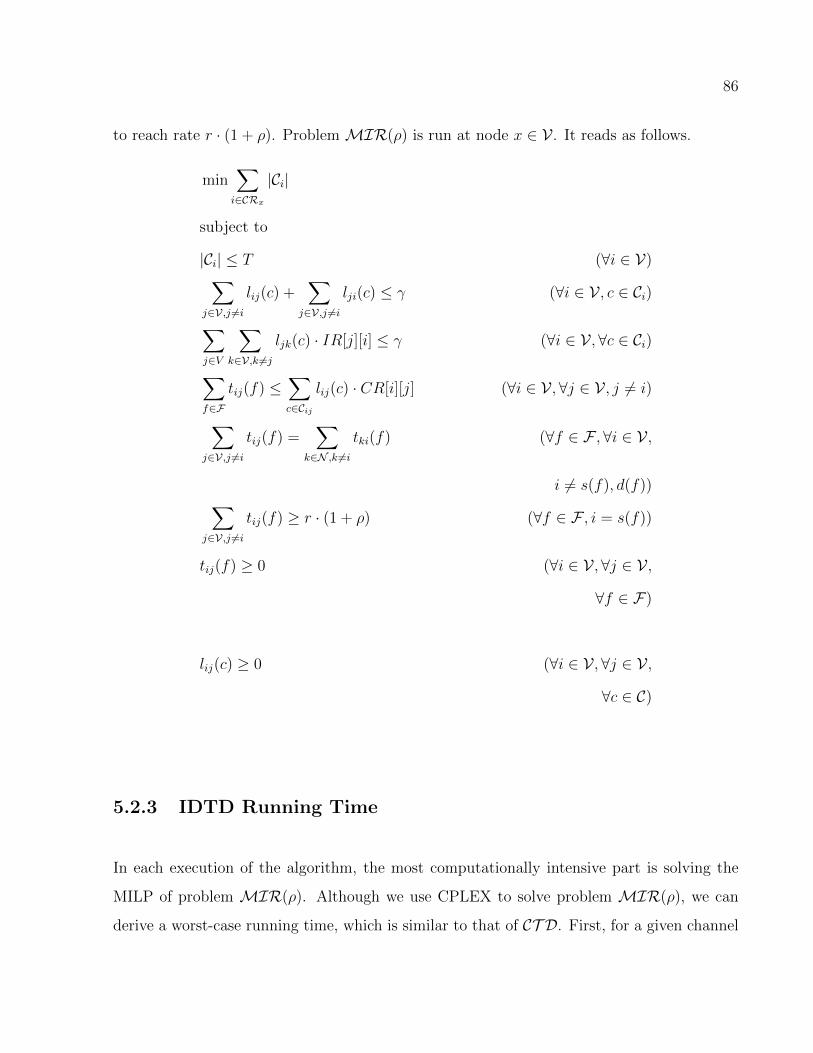
86

to reach rate r · (1 + ρ). Problem MIR(ρ) is run at node x ∈ V . It reads as follows.

min∑i∈CRx

|Ci|

subject to

|Ci| ≤ T (∀i ∈ V)∑j∈V,j 6=i

lij(c) +∑

j∈V,j 6=i

lji(c) ≤ γ (∀i ∈ V , c ∈ Ci)

∑j∈V

∑k∈V,k 6=j

ljk(c) · IR[j][i] ≤ γ (∀i ∈ V ,∀c ∈ Ci)

∑f∈F


lij(c) · CR[i][j] (∀i ∈ V ,∀j ∈ V , j 6= i)

∑j∈V,j 6=i

tij(f) =∑

k∈N ,k 6=i

tki(f) (∀f ∈ F ,∀i ∈ V ,

i 6= s(f), d(f))∑j∈V,j 6=i

tij(f) ≥ r · (1 + ρ) (∀f ∈ F , i = s(f))

tij(f) ≥ 0 (∀i ∈ V ,∀j ∈ V ,

∀f ∈ F)

lij(c) ≥ 0 (∀i ∈ V ,∀j ∈ V ,

∀c ∈ C)

5.2.3 IDTD Running Time

In each execution of the algorithm, the most computationally intensive part is solving the

MILP of problem MIR(ρ). Although we use CPLEX to solve problem MIR(ρ), we can

derive a worst-case running time, which is similar to that of CT D. First, for a given channel

87

assignment, we recognize that the dual problem ofMIR(ρ) is the max-flow problem, which

can be solved in polynomial time with an LP [50]. However, like problem CT D, the number

of possible channel assignments for MIR(ρ) to consider also grows exponentially with the

number of nodes, channels, and transceivers per node, causing the running-time complexity

of MIR to also grow exponentially.

Similar to CT D, the number of LPs required to solve MIR(ρ) is greatly reduced since the

TD adaptation is restricted to only using the transceivers not assigned independently of

traffic conditions. Additionally, problem MIR is solved with respect to a particular node,

and no node is allowed to change the assigned transceivers at any other node, which further

reduces the possible branches for MIR(ρ) to explore.

Unlike CT D, MIR(ρ) will be solved multiple times. The number of times is dependent on

the feasibility of MIR. If no improvement to the flow rate is infeasible, ρ is halved, and

the problem is tried again. If no improvement to the flow rate is feasible for any ρ ≥ ρmin,

problem MIR(ρ) is solved log2ρmax

ρmin= log2 ρmax − log2 ρmin times.

If improvement in flow rate is possible, the number of possible improvements must be incor-

porated into the running-time complexity analysis. Since the flow rate is strictly increasing

with each successful rate improvement (feasible solution) ofMIR(ρ), the algorithm will ter-

minate due to a finite amount of resources. The number of iterations required to terminate

the algorithm is dependent on ρmin. There is a tradeoff in the choice of ρmin: the lower it

is, the more likely the network will continue seeking adaptations and achieving a higher flow

rate, but this comes at the cost of increased running time.

5.3 Event-driven Simulation

In this section, we provide the details of the event-driven simulation used to evaluate how the

traffic-aware approach adapts the topology in an event-based scenario. Figure 5.2 outlines

the basic elements of the event-driven simulation.

88

Figure 5.2: Flow Diagram of Event-driven Simulation

The event-driven simulation is initialized with a TI assignment, which remains constant

throughout the simulation. Flow arrivals follow a Poisson process, where arrivals are indepen-

dently and identically (exponentially) distributed. The size of the flow follows a heavy-tailed

Pareto distribution similar to those adopted in [4–8].

Flow departure times are calculated from the end-to-end flow rate that the topology supports.

We analyze the performance of the TA approach using routing schemes that maximize the rate

of all flows without knowledge of each flow’s size. The point of the simulation is to evaluate

how an intelligent, TA channel assignment scheme can adapt the topology in an event-driven

scenario as compared to the numerical analysis of Chapter 3 and Chapter 4. The results of

the event-driven simulation show how flow service/completion times are affected by the TD

assignment.

The outline of the remainder of this section is as follows. First, we discuss the routing layer

used for calculating flow rate. Second, we define the set of TI and TD schemes we evaluate,

89

which includes a set of related approaches from the research literature used for comparison.

Lastly, we present and analyze the results of the simulation.

5.3.1 Independent Routing Layer

The focus of this dissertation is on TA channel assignment with the goal of adapting the

topology to support higher end-to-end flow rates. The TA assignment does not directly solve

the problem of routing or transmission scheduling, which are traditionally network layer or

medium access control (MAC) layer functions; however, to show how the TA assignment

affects the maximum flow rate, we use an MILP which routes flows over the multi-channel

topology created by the network’s channel assignment. We show that the TA assignment’s

effectiveness using two different routing schemes, both of which maximize flow rate fairly

among all flows, independently of each flow’s size. The following two schemes are used for

calculating the flow rate and the next departure time in the last step of the main simulation

loop. The motivation of using the two routing schemes is to show that our TA approach is

not tied to a specific routing approach.

5.3.1.1 Max-min Routing, MMR

The first routing scheme, which we denote as problem MMR, is a simple maximization of

the minimum flow rate. ProblemMMR is nearly identical to problem FM, but inMMR,

there is no TD channel assignment, causingMMR to reduce to a linear program (LP). This

means that the Ci terms are constants instead of channel assignment integer decision variables

as they are in FM. Problem MMR reads the same as FM with the noted exception of

the Ci terms becoming constants. (See Subsection 3.1.1 for details on the notation.)

90

max∑f∈F

wf · r

subject to

|Ci| ≤ T (∀i ∈ V)∑j∈V,j 6=i

lij(c) +∑

j∈V,j 6=i

lji(c) ≤ γ (∀i ∈ V , c ∈ C)

∑j∈V

∑k∈V,k 6=j

ljk(c) · IR[j][i] ≤ γ (∀i ∈ V ,∀c ∈ C)

∑f∈F


lij(c) · CR[i][j] (∀i ∈ V ,∀j ∈ V , j 6= i)

∑j∈V,j 6=i

tij(f) =∑

k∈N ,k 6=i

tki(f) (∀f ∈ F ,∀i ∈ V , i 6= s(f), d(f))

∑j∈V,j 6=i

tij(f) = r (∀f ∈ F , i = s(f))

tij(f) ≥ 0 (∀i ∈ V ,∀j ∈ V ,∀f ∈ F)

lij(c) ≥ 0 (∀i ∈ V ,∀j ∈ V ,∀c ∈ C)

5.3.1.2 Lexicographic Max-min Routing, LMMR

The second routing scheme, which we denote as problem LMMR, is a lexicographic max-min

routing approach similar to that adopted in [51] and [52]. The motivation for this approach

is that solving LMMR allows for flow rates on some of the flows to exceed the maximum

minimum, bottleneck flow rate if possible. In a distributed network of independent routers,

all flow rates may not be rate-limited by a single bottlenecked flow.

First, the lexicographic max-min routing approach finds the max-min flow rate, denoted as

r1, which is the same as in problem MMR, and due to the problem definition, there is a

91

flow that cannot exceed rate r1. The next step of LMMR is to set the rate of a single

flow that cannot exceed rate r1 to r1 for the remainder of the problem and to maximize the

minimum rate of the other flows, finding rate r2. Then, the flows corresponding to rates r1

and r2 are fixed, and the maximum minimum rate is found on the remaining flows, finding r3.

The lexicographic max-min routing approach continues this process and iteratively finds flow

rates r1, r2, r3, ..., r|F| where r1 ≤ r2 ≤ r3 ≤ ... ≤ r|F|. Overall, problem LMMR consists

of solving problem MMR |F| times, and at each iteration of solving a problem similar to

MMR, the resulting flow rate monotonically increases, giving a lexicographic ordering of

the flow rates supported by the topology.

Algorithm 4 Lexicographic Max-min

1: Ffixed ← ∅

2: r1 ← r solution of MMR using flow set F

3: f ← flow bottlenecked at rate r1

4: for i = 2 to |F| do

5: ri ← r solution of MMR using flow set F \ Ffixed with rates r1, ... , ri−1 fixed

6: f ← flow bottlednecked at rate ri

7: Ffixed ← Ffixed ∪ {f}

8: end for

5.3.2 TI and TD Simulation Configuration

We evaluate four configurations in our performance evaluation varying in the approaches

for TI and TD assignment. In approach (1), we adopt an optimal resource-minimized TI

assignment from Section 4.1 (also presented in Subsection 3.1.1) and the centralized TD

assignment presented in Section 5.1. We denote approach (1) as RM, CT D. Approach (2)

adopts the same approach for TI assignment as approach (1) but uses the IDTD algorithm for

TD assignment. Approach (3) adopts the distributed resource-minimized channel assignment

(RMCA), which is presented in Section 4.3, for TI assignment and the IDTD algorithm

92

Table 5.1: Summary of approaches for the event-driven simulation: Traffic-independent as-

signment occurs and is followed by TD assignment of those resources not traffic-independently

assigned. The TD assignment adapts based on the traffic demands, but the TI assignment

remains constant.

Approach Configuration TI Assignment TD Assignment

(1): RM, CT D Optimal resource-minimized Centralized TD

(2): RM, IDTD Optimal resource-minimized Distributed TD

(3): RMCA, IDTD Distributed resource-minimized Distributed TD

(4): CM(α = 1) Connectivity-maximized None

for TD assignment. Approaches (2) and (3) are denoted RM, IDTD and RMCA, IDTD,

respectively. Approach (4), which is denoted CM(α = 1), adopts a connectivity-maximized

TI connectivity using all of the network’s transceivers with no TD approach since there are

no resources conserved for TD assignment. Approach (4) is formulated in Subsection 3.1.2

with parameter α = 1. We evaluate each approach with both MMR and LMMR routing

approaches. Table 5.1 summarizes the approaches used in the event-driven performance

evaluation.

5.3.3 Results

The event-driven simulation follows the procedure outlined in Figure 5.2. The number of

nodes, |V|, is 25. Node placement is (uniformly) random in a rectangular area of dimensions

2 by 12. The communication range, rcomm, is 0.8. The parameters for the set of nodes

V , the rectangular area, and rcomm provide a scenario in which the network diameter is

typically spanning 5 to 6 hops. We vary the number transceivers per node, T , from 2 to 4.

Rate parameter γ = 10 megabits per second (Mbps). Traffic-demand size follows a Pareto

93

distribution3 with k = 1 kB and σ = 0.43. The CDF is shown in Figure 5.1.

For the centralized TD, η = 25 kB, and in the distributed TD scheme, η = 16 kB. The

parameter ρ is initially set to 20% in each run of the distributed TD algorithm. Parameter

ρmax = 20% and ρmin = 1%. The txtimeout = 2.5 seconds, and parameter flowwindow = 2.5

seconds of time. The IDTD algorithm executes every 2 seconds.

Figure 5.3 shows the performance of the set of schemes usingMMR routing. Subfigure 5.3a

shows the mean flow rate for all flows for each scheme in our evaluation, and Subfigure 5.3b

shows the number of transceivers enabled and disabled during TD adaptations. We see that

the performance of approaches (1)-(3) are similar to one another in scenarios with T = 3 and

T = 4. This shows that the IDTD algorithm is providing a set appropriate of adaptations

to reach a similar flow rate to that of CT D, the centralized approach. Furthermore, algo-

rithm IDTD has an order of magnitude fewer adaptations of enabling and disabling fewer

transceivers while achieving near the rate of CT D. Approaches (1) - (3) greatly outperform

scenario (4), the strictly TI assignment.

For scheme (3) with T = 2, the mean flow rate is higher than scheme (2) and significantly

higher than scheme (1). The difference from scheme (2) to (3) is from the suboptimal

resource conservation in scheme (3) occurring in the TI stage of assignment. These results

are consistent with those presented in Chapter 4 for scenarios where RMCA assigned 1.6

transceivers on average per node using RMCA as compared to 1.4 transceivers per node

using RM. The difference is enough to cause a significantly lower flow rate because there

are only on average 0.4 transceivers per node conserved for TD allocation.

However, for scenarios with T = 3 and T = 4, the slight increase in the number of transceivers

assigned traffic-independently leads scheme (3) to achieve a slightly higher rate than scheme

(2). As shown in Chapter 4, using RMCA with T = 3 and T = 4, there are on average

3The CDF of the Pareto distribution is F (x) = P [X ≤ x] = 1−(kx

)σwhere k is the minimum value of X

and σ is the shaping parameter.

94

2 3 40

1

2

3

4

5

6

7

Mean Flow Rate (MMR Routing)

Number of Transceivers per Node

Me

ga

bits p

er

se

co

nd

(M

bp

s)

RM, CTD

RM, IDTD

RMCA, IDTD

CM(α = 1)

(a) Mean Flow Rate

1 2 3 40

100

200

300

400

500

600

700

800

900

1000

1100

Co

un

t o

f T

ran

sce

ive

r A

ctio

ns

T=2

Trx Enabled

Trx Disabled

1 2 3 40

200

400

600

800

1000

1200

1400

1600

1800

T=3

Trx Enabled

Trx Disabled

1 2 3 40

500

1000

1500

2000

2500

T=4

Trx Enabled

Trx Disabled

(b) Transceivers Enabled and Disabled,

Schemes Labeled According to Table 5.1

10−4

10−3

10−2

10−1

100

101

102

0

0.1

0.2

0.3

0.4

0.5

0.6

0.7

0.8

0.9

1

CDF of Flow Completion Time (T = 2, MMR Routing)

Seconds

Cum

ula

tive P

robabili

ty

RM, CTD

RM, IDTD

RMCA, IDTD

CM(α = 1)

(c) CDF of Flow Completion Time with T = 2

10−4

10−3

10−2

10−1

100

101

102

0

0.1

0.2

0.3

0.4

0.5

0.6

0.7

0.8

0.9

1


Seconds

Cum

ula

tive P

robabili

ty

RM, CTD

RM, IDTD

RMCA, IDTD

CM(α = 1)

(d) CDF of Flow Completion Time with T = 3

10−4

10−3

10−2

10−1

100

101

102

0

0.1

0.2

0.3

0.4

0.5

0.6

0.7

0.8

0.9

1


Seconds

Cum

ula

tive P

robabili

ty

RM, CTD

RM, IDTD

RMCA, IDTD

CM(α = 1)

(e) CDF of Flow Completion Time with T = 4

2 3 40

0.2

0.4

0.6

0.8

1

1.2

1.4

1.6

1.8Mean Flow Completion Time (MMR Routing)


Se

co

nd

s

RM, CTD

RM, IDTD

RMCA, IDTD

CM(α = 1)

(f) Mean Completion Time

Figure 5.3: Comparison of Schemes with MMR Routing

95

1.4 and 2.4 transceivers per node conserved for TD allocation, respectively, and this amount

of transceiver conservation is shown to be sufficient to allow within a few percent of the

optimum flow rate. Given that IDTD is conservative in its traffic-driven adaptations, as

shown in Subfigure 5.3b, the slightly higher amount of transceivers allocated independently

of traffic conditions in scheme (3) (by using RMCA as opposed to RM helps scheme (3)

outperform (2) with T = 3 and T = 4.

While analyzing Subfigures 5.3a and 5.3b, we see that the slight increase in flow rate while

using CT D over IDTD comes at the cost of an order of magnitude larger number of transceiver

actions (enabling or disabling transceivers) throughout the event-driven simulation. Schemes

(2) and (3), which use the IDTD algorithm, can achieve similar performance in terms of flow

completion time as compared to scheme (1). This suggests that the additional adaptations

from CT D have limited benefit since there is insignificant benefit in terms of increasing mean

rate or decreasing flow completion time.

Subfigures 5.3c, 5.3d, and 5.3e show the CDF of flow completion time for scenarios with

T = 2 , T = 3, and T = 4, respectively, and Subfigure 5.3f shows the mean flow completion

time for all scenarios. For the most part, the results of Subfigures 5.3c - 5.3f are consistent

with the mean flow rate of Subfigure 5.3a. Scheme (3) has a higher proportion of flows

requiring 80 ms or less to complete than schemes (1) and (2) with T = 3 and T = 4. This

is due to RMCA allocating slightly more transceivers independently of traffic-conditions, as

noted previously. Also, since the IDTD algorithm allows transceivers allocated in response

to flows consisting of more than η kB to remain enabled if they are used for any flow, the

traffic-driven adaptations of IDTD can benefit flows consisting of less than η kB.

Figure 5.4 shows the performance of the set of schemes using LMMR routing. For the most

part, the results are consistent with that of Figure 5.3 andMMR routing. Overall, the mean

flow rate is increased for all schemes, and this translates into lower flow completion times for

all schemes. This is expected since given the same set of parameters (i.e., channel assignment

and traffic flows), LMMR routing finds flow rates that are lexicographically greater than or

96

2 3 40

1

2

3

4

5

6

7

8

Mean Flow Rate (LMMR Routing)


Me

ga

bits p

er

se

co

nd

(M

bp

s)

RM, CTD

RM, IDTD

RMCA, IDTD

CM(α = 1)

(a) Mean Flow Rate

1 2 3 40

100

200

300

400

500

600

700

800

900

1000

1100

Co

un

t o

f T

ran

sce

ive

r A

ctio

ns

T=2

Trx Enabled

Trx Disabled

1 2 3 40

200

400

600

800

1000

1200

1400

1600

1800

T=3

Trx Enabled

Trx Disabled

1 2 3 40

500

1000

1500

2000

2500

T=4

Trx Enabled

Trx Disabled

(b) Transceivers Enabled and Disabled,

Schemes Labeled According to Table 5.1

10−4

10−3

10−2

10−1

100

101

102

0

0.1

0.2

0.3

0.4

0.5

0.6

0.7

0.8

0.9

1

CDF of Flow Completion Time (T = 2, LMMR Routing)

Seconds

Cum

ula

tive P

robabili

ty

RM, CTD

RM, IDTD

RMCA, IDTD

CM(α = 1)

(c) CDF of Flow Completion Time with T = 2

10−4

10−3

10−2

10−1

100

101

102

0

0.1

0.2

0.3

0.4

0.5

0.6

0.7

0.8

0.9

1


Seconds

Cum

ula

tive P

robabili

ty

RM, CTD

RM, IDTD

RMCA, IDTD

CM(α = 1)

(d) CDF of Flow Completion Time with T = 3

10−4

10−3

10−2

10−1

100

101

102

0

0.1

0.2

0.3

0.4

0.5

0.6

0.7

0.8

0.9

1


Seconds

Cum

ula

tive P

robabili

ty

RM, CTD

RM, IDTD

RMCA, IDTD

CM(α = 1)

(e) CDF of Flow Completion Time with T = 4

2 3 40

0.2

0.4

0.6

0.8

1

1.2

1.4

1.6

Mean Flow Completion Time (LMMR Routing)


Se

co

nd

s

RM, CTD

RM, IDTD

RMCA, IDTD

CM(α = 1)

(f) Mean Completion Time

Figure 5.4: Comparison of Schemes with LMMR Routing

97

equal to flow rates found by MMR. The most notable difference between Figures 5.3 and

5.4 is with scheme (4), which seems to benefit the most from LMMR routing. In Subfigures

5.4c - 5.4e, scheme (4) has the highest proportion of flows requiring 1 ms or less to complete.

These flows most-likely consist of only a few packets or less. This is expected since scheme

(4) has all its resources allocated traffic-independently, and the bottleneck rate, r1, will not

prevent scheme (4) from achieving higher flow rates with other flows with LMMR routing

as it does when using MMR routing.

5.4 Conclusion

In this chapter, we focus on the second stage of the TA approach: the traffic-driven stage. We

formulate a centralized approach with problem CT D, which follows an MILP and maximizes

end-to-end flow rate on the flows that are of the highest and most significant demand. We

develop the iterative, distributed TD (IDTD) approach with a similar goal. In the distributed

approach, nodes adapt their local channel assignment to organically morph the topology

and augment the topology with additional paths that increase end-to-end flow rate. In this

approach, nodes sense their environment and adapt locally to achieve a higher network utility,

following the ideals of cognitive networking [2].

We define various combinations traffic-independent schemes from Chapter 4 and traffic-driven

schemes, presented in this chapter, as well as a few popular approaches from the research

literature, and we evaluate these schemes using an event-driven simulation. We find that

employing the IDTD approach yields similar flow completion time as compared to employing

the CT D approach while having an order of magnitude fewer adaptations.

Although the results from this chapter are promising, the CT D and IDTD algorithms rely on

using an MILP solver. Developing an algorithm for selecting specific flow-rate augmenting

paths is left as future work. Developing such an algorithm would make this approach more

98

viable for implementation on systems with limited computing power and battery life (i.e.,

mobile systems).

Chapter 6

Conclusion

In this chapter, we conclude the dissertation. In Section 6.1, we summarize the contributions

of this dissertation, providing some of the main conclusions of each chapter. In Section 6.2,

we outline potential future work in this area.

6.1 Research Contributions

The primary research contribution of this dissertation is proposing a new method of channel

assignment for cognitive radio networks (CRNs) that incorporates two complementary ap-

proaches of channel assignment: traffic-independent (TI) and traffic-driven (TD) assignment.

We propose that some transceivers be enabled and assigned to a channel independently of

traffic conditions and some transceivers be enabled in response to traffic conditions. The TI

assignment is designed to maintain stable, baseline network connectivity. In contrast, the

TD assignment is intended to adapt the network’s topology (through enabling additional

links) to better support the end-to-end flow of traffic. We propose that a minimum number

of transceivers be assigned independently of traffic conditions in order for the network to be

more flexible in its adaptation to traffic demands. By conserving resources initially with the

99

100

TI assignment, the network has more resources for any TD assignment, and more resources

allocated in the TD assignment translates to higher end-to-end flow rate. This proposal was

illustrated in Figure 1.4.

6.1.1 Balance of TI and TD Resource Allocation

In our first contribution, we examined the fundamental tradeoff in the proportion of resources

allocated independently of traffic conditions and those resources allocated in response to

traffic conditions. As more resources are allocated independently of traffic conditions, the

network can achieve higher connectivity, but as more resources are allocated in response

to traffic demands, the network can support higher end-to-end flow rate. The goal is to

investigate what resource allocation best balances both the desire for maximizing flow rate

and the need for the network to be adequately connected.

We formulated the problem as a two-stage, mixed-integer linear program (MILP), with the

first stage being a TI assignment and the second stage being a TD assignment. In the first

(TI) stage, connectivity is maximized using a proportion, α, of the network’s transceivers,

using an MILP denoted CM(α). In the second (TD) stage, channels are assigned using the

remaining 1 − α proportion of the network’s transceivers to maximize end-to-end flow rate,

using an MILP denoted problem FM.

We find that connectivity increases monotonically as a function of α, but beyond a cer-

tain point there are diminishing returns in terms of additional network connectivity gained

through the allocation of additional transceivers for connectivity. Also, we see that the max-

imum achievable end-to-end flow rate decreases monotonically as a function of α, but beyond

a point the flow rate diminishes more quickly. We find that, at the values of α for which

the network graph has a baseline connectivity, there is little, if any, decrease in flow rate as

compared to the theoretical maximum flow rate (when α = 0), supporting our central idea of

a resource-minimized TI assignment followed by a TD allocation. This contribution follows

from our work in [9] and was described in Chapter 3.

101

6.1.2 Resource-Minimized TI Channel Assignment

In our second contribution, we examined the problem of TI channel assignment and devel-

oped a set of approaches that follow our proposal of a resource-minimized TI assignment.

Our approach is in contrast to much of the research literature, which focuses on strategies of

assigning channels to all available transceivers with the typical objective of either maximiz-

ing connectivity or minimizing interference. However, we compared our approach to other

approaches in the research literature that do minimize the amount of resources allocated

traffic-independently to a degree.

The motivation for a resource-minimized TI approach is two-fold. The first motivation is that

energy is conserved, since there is a non-negligible cost in energy for each transceiver that

is activated and tuned to a channel. The second motivation, as outlined previously, is that,

by initially conserving resources, there can be a stronger dynamic TD response to changing

traffic stimuli through subsequent enabling of and channel assignment to transceivers.

We formulated an optimal approach to resource-minimized TI assignment, with problem

RM, which follows an MILP. Also, we develop two heuristic algorithms. One is called

centralized resource-minimized channel assignment (RMCA), while the other is called dis-

tributed RMCA. We found that our approaches perform much closer to optimal than other

proposed approaches in the research literature in terms of the number of channel assignments

necessary to maintain network connectivity. We also found that our proposed approaches

exhibit a lower conflict degree as compared to other approaches.

To fairly compare each TI approach’s impact on achievable flow rate, problem FM is solved

to assign any transceivers not assigned traffic-independently to maximize flow rate. We found

that our approaches are able to achieve a higher maximum flow rate than other approaches

due to using fewer transceivers for TI channel assignment. Furthermore, our approaches

achieved within a small percentage of the optimal (the solutions of both RM and FM) flow

rate averaged across all evaluated scenarios. This contribution is an extension from our work

in [10] and was described in Chapter 4.

102

6.1.3 Traffic-driven Channel Assignment

In our third contribution, we examined the problem of TD channel assignment. Closely

aligned with the ideals of cognitive networking, we proposed an approach that senses traffic

conditions as well as channel and transceiver usage and intelligently adapts the channel

assignment locally to better support the end-to-end flow of traffic. The goal is for nodes

to act independently and organically adapt the topology over time in a way that maintains

network connectivity but optimizes the topology based on the flow demand.

We developed an optimal centralized approach to TD assignment in CT D. Also, we developed

the iterative, distributed TD (IDTD) approach, in which each node runs a background process

that periodically executes, aggregating traffic statistics over a sliding window of time, which

gives nodes the ability to sense which flows are of more substantial demand. Then, the nodes

sense if any of the substantial flows are bottlenecked and assigns channels locally to alleviate

any bottlenecks if possible. The motivation for not optimizing based on all flows is that

there is a non-negligible cost in terms of energy associated with enabling a transceiver and

tuning it to a channel, so the benefit of making an adaptation to a flow of light demand (e.g.

a one-packet flow) is not worth the cost of enabling and assigning a transceiver. We argue

that light flow demands can be served using the resources dedicated for maintaining network

connectivity assigned traffic-independently.

We developed an event-driven simulation to showcase the how the traffic-aware approach

performs in an event-driven scenario. We showed that the approaches using IDTD assignment

perform close to the optimal CT D approach in the majority of the evaluated scenarios in

terms of flow rate and flow completion time. Also, these approaches greatly outperform the

common approach of assigning all channels independently of traffic conditions. Lastly, we

found that the IDTD approach enabled and disabled fewer transceivers while adapting the

topology than does the optimal approach by an order of magnitude. This contribution was

described in Chapter 5 and follows from our first attempt at a similar problem in [11].

103

6.2 Future Work

Although this dissertation provides an evaluation of a promising two-stage approach to chan-

nel assignment in CRNs, there are a few areas to extend the contributions of this body of

work. First, we focus on the limitations of our approach shown in the performance evalua-

tions presented in this dissertation, and second, we focus on broader issues of expanding this

work.

6.2.1 Enhancements to the RMCA and IDTD Approaches

In Chapter 5, there was a subtle drop-off in flow-rate performance when comparing the

optimal TI-TD (RM-CT D) approach with the (distributed) RMCA-IDTD approach. The

drop-off was acute in only the scenarios with two transceivers per node. Since RMCA allo-

cates on average 1.6 transceivers per node to traffic-independent connectivity (as opposed to

1.2 using the optimal approach of RM), we attribute the decrease in flow rate to the lack

of transceivers conserved for TD assignment. These results are also consistent with those in

Chapter 4 where the gap between the maximum flow rate with distributed RMCA and the

RM (Optimal RMCA) was largest in scenarios with T = 2. It may be possible to improve

the distributed RMCA approach by reducing the number of transceivers dedicated for main-

taining network connectivity in hope of improving the TD response and maximum flow rate.

It may be possible to have a subsequent phase that eliminates transceiver assignments that

are deemed unnecessary to maintain network connectivity.

Another area of possible improvement is with the IDTD algorithm. The IDTD algorithm re-

lies on an MILP solver. Using a solver may require a significant amount of resources that may

inhibit the adoption of the IDTD algorithm in some resource-limited systems (e.g. mobile

systems). In [11], we developed the channel assignment based on routing decisions (CARD)

104

algorithm for a similar problem; however, the CARD algorithm searches for assigning chan-

nels to enable additional node-disjoint paths, whereas the IDTD algorithm seeks any kind of

additional link or path that could increase the current flow rate. Overall, the approach devel-

oped in [11] and the contributions of Chapter 5 indicate progress in developing a distributed

algorithm without using a solver for enabling additional, flow-rate augmenting paths.

6.2.2 Expansion of Work

A major premise of this dissertation is that actions of enabling, tuning, and operating

transceivers have non-negligible costs in terms of time and energy consumed, and that, in

general, fewer transceiver actions is better. In practice, it may be necessary to do a more

rigorous cost-benefit analysis in order to more accurately judge the tradeoffs involved. The

major factor limiting our research in this area is the lack of a standard multi-transceiver

or multi-radio platform. Specifically, the costs are impacted by designs that have not been

standardized. Design considerations include frequency filtering stages (i.e., the number and

location(s) of filters) and power amplifier location(s). Also, the multi-transceiver device may

have frequency-dependent performance issues such as non-uniform channel tuning times, un-

equal energy consumption per band, and non-uniform power output across frequency bands.

Defining a radio platform and characterizing its performance would allow us to more accu-

rately assess the costs and benefits associated with any of the transceiver actions.

Another more broad topic for expanding this research involves addressing dynamics other

than traffic-related dynamics. The focus of the resource allocation strategy presented in

this dissertation was geared toward handling the dynamics of changing traffic conditions.

Additional dynamics that could be addressed involve node mobility or node failure as well as

dynamically available channels as in a dynamic spectrum access (DSA) environment. These

additional dynamics could prompt adaptations in the traffic-independent allocation in order

to maintain connectivity through various traffic-independent dynamics, a topic not addressed

in this dissertation.

Bibliography

[1] J. Reed, Software radio: a modern approach to radio engineering. Prentice Hall Profes-

sional, 2002.

[2] R. Thomas, D. Friend, L. DaSilva, and A. MacKenzie, “Cognitive Networks: Adaptation

and Learning to Achieve End-to-end Performance Objectives,” IEEE Communications

Magazine, vol. 44, no. 12, pp. 51–57, 2007.

[3] M. Lawler, “Wireless to the Nth Degree,” AFCEA SIGNAL Online Magazine, 2006.

[4] B. Mah, “An Empirical Model of HTTP Network Traffic,” in Proceedings of IEEE Inter-

national Conference on Computer Communications (INFOCOM), vol. 2, pp. 592–600,

IEEE, 1997.

[5] R. Pang, M. Allman, M. Bennett, J. Lee, V. Paxson, and B. Tierney, “A First Look at

Modern Enterprise Traffic,” in Proceedings of ACM SIGCOMM Conference on Internet

Measurement, pp. 1–14, ACM, 2005.

[6] C. Mueller, “Analysis of Interactions between Internet Data Traffic Characteristics and

Coordinated Multipoint Transmission Schemes,” in Proceedings of IEEE Wireless Com-

munications and Networking Conference (WCNC), pp. 263–268, IEEE, 2011.

[7] L. Shuai, G. Xie, and J. Yang, “Characterization of HTTP Behavior on Access Networks

in Web 2.0,” in Proceedings of IEEE International Conference on Telecommunications

(ICT), pp. 1–6, IEEE, 2008.

105

106

[8] “Let’s Make the Web Faster.” http://code.google.com/speed/articles/web-metrics.html,

2012.

[9] R. Irwin, A. B. MacKenzie, and L. DaSilva, “Traffic-Aware Channel Assignment for

Multi-radio Wireless Networks,” in Proceedings of IFIP International Conference on

Networking, 2012.

[10] R. Irwin, A. B. MacKenzie, and L. DaSilva, “Resource-Minimized Channel Assignment

for Multi-transceiver Wireless Networks,” in Proceedings of IEEE Global Communica-

tions Conference (GLOBECOM), 2011.

[11] R. Irwin and L. DaSilva, “Channel Assignment Based on Routing Decisions (CARD):

Traffic-Dependent Topology Control for Multi-Channel Networks,” in Proceedings of

IEEE International Conference on Communications (ICC) CogNet Workshop, 2009.

[12] G. Jakllari, S. Ramanathan, J. Redi, D. Coffin, W. Tetteh, J. Burgess, and R. Irwin,

“Distributed Assignment of Frequency Channels to Transceivers over Dynamic Spec-

trum,” Sept. 16 2010. US Patent App. 20,100/232,372.

[13] T. Chen, H. Zhang, G. Maggio, and I. Chlamtac, “CogMesh: A Cluster-based Cog-

nitive Radio Network,” in Proceedings of IEEE Dynamic Spectrum Access Networks

(DySPAN), pp. 168–178, 2007.

[14] M. Shin, S. Lee, and Y. ah Kim, “Distributed Channel Assignment for Multi-radio

Wireless Networks,” in Proceedings of IEEE Mobile Adhoc and Sensor Systems (MASS),

pp. 417–426, 2006.

[15] A. P. Subramanian, H. Gupta, S. R. Das, and J. Cao, “Minimum Interference Chan-

nel Assignment in Multiradio Wireless Mesh Networks,” IEEE Transactions on Mobile

Computing, vol. 7, no. 12, pp. 1459–1473, 2008.

[16] B. Ko, V. Misra, J. Padhye, and D. Rubenstein, “Distributed Channel Assignment in

107

Multi-radio 802.11 Mesh Networks,” in Proceedings of IEEE Wireless Communications

and Networking Conference (WCNC), pp. 3978–3983, IEEE, 2007.

[17] A. Plummer Jr, T. Wu, and S. Biswas, “A Localized and Distributed Channel Assign-

ment Framework for Cognitive Radio Networks,” in First International Workshop on

Cognitive Wireless Networks, ACM, 2007.

[18] J. Tang, G. Xue, and W. Zhang, “Interference-aware Topology Control and QoS Routing

in Multi-channel Wireless Mesh Networks,” in Proceedings of ACM International Sym-

posium of Mobile Ad Hoc Networking and Computing (MOBIHOC), pp. 68–77, ACM,

2005.

[19] M. Marina, S. Das, and A. Subramanian, “A Topology Control Approach for Utilizing

Multiple Channels in Multi-radio Wireless Mesh Networks,” Computer Networks, 2010.

[20] K. Ramachandran, E. Belding, K. Almeroth, and M. Buddhikot, “Interference-aware

Channel Assignment in Multi-radio Wireless Mesh Networks,” in Proceedings of IEEE

International Conference on Computer Communications (INFOCOM), vol. 6, pp. 1–12,

IEEE, 2006.

[21] D. Grace, T. Tozer, and A. Burr, “Reducing Call Dropping in Distributed Dynamic

Channel Assignment Algorithms by Incorporating Power Control in Wireless Ad Hoc

Networks,” IEEE Journal on Selected Areas in Communications, vol. 18, no. 11,

pp. 2417–2428, 2000.

[22] T. ElBatt and A. Ephremides, “Joint Scheduling and Power Control for Wireless Ad Hoc

Networks,” IEEE Transactions on Wireless Communications, vol. 3, no. 1, pp. 74–85,

2004.

[23] J. Deaton, S. Ahmad, U. Shukla, R. Irwin, L. DaSilva, and A. MacKenzie, “Evaluation

of Dynamic Channel and Power Assignment for Cognitive Networks,” Wireless Personal

Communications, vol. 57, pp. 5–18, 2011.

108

[24] G. Kulkarni and M. Srivastava, “A Channel Assignment Scheme for FDMA Based Wire-

less Ad Hoc Networks in Rayleigh Fading Environments,” in Proceedings of IEEE Con-

ference on Vehicular Technology Conference (VTC), vol. 2, pp. 1082–1085, IEEE, 2002.

[25] C. Chin, M. Sim, and S. Olafsson, “A Dynamic Channel Assignment Sstrategy via Power

Control for Ad-hoc Network Systems,” in Proceedings of IEEE Conference on Vehicular

Technology Conference (VTC), pp. 3006–3010, IEEE, 2007.

[26] G. Foschini and Z. Miljanic, “A Simple Distributed Autonomous Power Control Algo-

rithm and its Convergence,” IEEE Transactions on Vehicular Technology, vol. 42, no. 4,

pp. 641–646, 1993.

[27] L. Tassiulas and A. Ephremides, “Dynamic Server Allocation to Parallel Queues with

Randomly Varying Connectivity,” IEEE Transactions on Information Theory, vol. 39,

no. 2, pp. 466–478, 1993.

[28] M. Neely and R. Urgaonkar, “Optimal backpressure routing for wireless networks with

multi-receiver diversity,” Ad Hoc Networks, vol. 7, no. 5, pp. 862–881, 2009.

[29] R. Urgaonkar and M. Neely, “Opportunistic Scheduling with Reliability Guarantees in

Cognitive Radio Networks,” IEEE Transactions on Mobile Computing, vol. 8, no. 6,

pp. 766–777, 2009.

[30] U. Shukla, “Backpressure Policies for Wireless Ad Hoc Networks,” M.S. Thesis, 2010.

[31] M. Alicherry, R. Bhatia, and L. Li, “Joint Channel Assignment and Routing for Through-

put Optimization in Multi-Radio Wireless Mesh Networks,” in Proceedings of ACM

International Conference on Mobile Computing and Networking (MOBICOM), p. 72,

ACM, 2005.

[32] X. Lin and S. Rasool, “A Distributed Joint Channel-Assignment, Scheduling and Rout-

ing Algorithm for Multi-channel Ad-hoc Wireless Networks,” in Proceedings of IEEE

109

International Conference on Computer Communications (INFOCOM), pp. 1118–1126,

IEEE, 2007.

[33] Y. Shi and Y. Hou, “A Distributed Optimization Algorithm for Multi-hop Cognitive

Radio Networks,” in Proceedings of IEEE International Conference on Computer Com-

munications (INFOCOM), pp. 1292–1300, IEEE, 2008.

[34] W. So, J. Walrand, and J. Mo, “McMAC: A Parallel Rendezvous Multi-channel MAC

Protocol,” in Proceedings of IEEE Wireless Communications and Networking Conference

(WCNC), pp. 334–339, IEEE, 2007.

[35] C. Cordeiro and K. Challapali, “C-MAC: A Cognitive MAC Protocol for Multi-channel

Wireless Networks,” in Proceedings of IEEE International Conference on Dynamic Spec-

trum Access Networks (DySPAN), pp. 147–157, IEEE, 2007.

[36] S. Wu, C. Lin, Y. Tseng, and J. Sheu, “A New Multi-channel MAC Protocol with On-

demand Channel Assignment for Multi-hop Mobile Ad Hoc Networks,” in Proceeding

of IEEE International Symposium on Parallel Architectures, Algorithms and Networks

(I-SPAN), pp. 232–237, IEEE, 2002.

[37] C. Xu, G. Li, W. Cheng, and Z. Yang, “Multi-transceiver Multiple Access (MTMA) for

Mobile Wireless Ad Hoc Networks,” in Proceedings of IEEE International Conference

on Communications (ICC), vol. 5, pp. 2932–2936, IEEE, 2005.

[38] A. Tzamaloukas, “Channel-hopping Multiple Access,” in Proceeding of IEEE Interna-

tional Conference Communications (ICC), vol. 1, pp. 415–419, IEEE, 2002.

[39] A. Tzamaloukas, “A Receiver-initiated Collision-avoidance Protocol for Multi-channel

Networks,” in Proceedings of IEEE International Conference on Computer Communi-

cations (INFOCOM), vol. 1, pp. 189–198, IEEE, 2002.

[40] N. Theis, R. Thomas, and L. DaSilva, “Rendezvous for Cognitive Radios,” IEEE Trans-

actions on Mobile Computing, vol. 10, no. 2, pp. 216–227, 2011.

110

[41] P. Bahl, R. Chandra, and J. Dunagan, “SSCH: Slotted Seeded Channel Hopping for

Capacity Improvement in IEEE 802.11 Ad-hoc Wireless Networks,” in Proceedings of

IEEE International Conference on Mobile Computing and Networking (MOBICOM),

pp. 216–230, ACM, 2004.

[42] J. Chen, S. Sheu, and C. Yang, “A New Multichannel Access Protocol for IEEE 802.11

Ad Hoc Wireless LANs,” in Proceedings of IEEE Conference on Personal, Indoor and

Mobile Radio Communications (PIMRC), vol. 3, pp. 2291–2296, IEEE, 2004.

[43] P. Porwal and M. Papadopouli, “On-demand Channel Switching for Multi-channel Wire-

less MAC Protocols,” in 12th European Wireless Conference, Technical Report TR04-

024, University of North Carolina at Chapel Hill, 2004.

[44] P. Kyasanur and N. Vaidya, “Capacity of Multi-channel Wireless Networks: Impact of

Number of Channels and Interfaces,” in Proceedings of the 11th annual international

conference on Mobile computing and networking, pp. 43–57, ACM, 2005.

[45] J. Mo, H. So, and J. Walrand, “Comparison of Multichannel MAC Protocols,” IEEE

Transactions on Mobile Computing, vol. 7, no. 1, pp. 50–65, 2007.

[46] H. Skalli, S. Das, L. Lenzini, and M. Conti, “Traffic and Interference Aware Channel

Assignment for Multi-radio Wireless Mesh Networks,” in Proceedings of ACM Inter-

national Conference on Mobile Computing and Networking (MOBICOM), pp. 15–26,

ACM, 2007.

[47] A. Raniwala, K. Gopalan, and T. Chiueh, “Centralized Channel Assignment and Rout-

ing Algorithms for Multi-channel Wireless Mesh Networks,” in Proceedings of ACM

International Conference on Mobile Computing and Communications Review (MCR),

vol. 8, (New York, NY, USA), pp. 50–65, ACM, 2004.

[48] “Calculate Maximum Flow in Directed Graph - MATLAB.”

http://www.mathworks.com/help/toolbox/bioinfo/ref/graphmaxflow.html, 2012.

111

[49] A. Goldberg and R. Tarjan, “A New Approach to the Maximum-flow Problem,” Journal

of the ACM (JACM), vol. 35, no. 4, pp. 921–940, 1988.

[50] M. Bazaraa, J. Jarvis, and H. Sherali, Linear Programming and Network Flows. Wiley-

Interscience, 2011.

[51] Y. Hou, Y. Shi, and H. Sherali, “On Lexicographic Max-min Node Lifetime for Wireless

Sensor Networks,” in Proceedings of IEEE International Conference on Communications

(ICC), vol. 7, pp. 3790–3796, IEEE, 2004.

[52] X. Wang, K. Kar, and J. Pang, “Lexicographic Max-min Fair Rate Allocation in Random

Access Wireless Networks,” in Proceedings of IEEE Conference on Decision and Control,

pp. 1294–1300, IEEE, 2006.

tra c-aware channel assignment for multi-transceiver

Documents