Toxic Release Inventoriesand Green Consumerism:

Empirical Evidence from Canada

WERNER ANTWEILER

University of British ColumbiaFaculty of Commerce and Business Administration

KATHRYN HARRISON

University of British ColumbiaDepartment of Political Science

January 2001

Abstract

We investigate the empirical relevance of green consumerism as a reaction to the dissemina-tion of information through toxic relase inventories. Assuming that consumers cannot attributepollution to individual products from a multi-product firm, we identify the effect from greenconsumerism through intra-firm inter-plant spillover effects in pollution abatement when con-sumers reduce demand equally across all product lines of the multi-product firm. We subject thepredictions from a simple theoretical model to empirical tests using 1993-98 panel data fromCanada’s National Pollutant Release Inventory (NPRI) in conjunction with related census data.We adjust our analysis for the toxicity of pollutants. The empirical results establish that greenconsumerism “works”: the dissemination of information through toxic release inventories pos-itively affects pollution abatement activities of firms.

JEL Codes: Q2,R3

Proposed Running Title: Green Consumerism in Canada

Corresponding author is Antweiler, University of British Columbia, Faculty of Commerce and Business Adminis-tration, 2053 Main Mall, Vancouver, BC, V6T 1Z2, Canada. Phone: 604-822-8484. Fax: 604-822-8477. E-mail:werner@economics.ca. Antweiler gratefully acknowledges financial support from Canada’s Social Sciences and Hu-manities Research Council and UBC’s W. Maurice Young Entrepreneurship and Venture Capital Research Centre. Har-rison: University of British Columbia, Department of Political Science, 1866 Main Mall, Vancouver, BC, V6T 1Z1,Canada. Email: khar@interchange.ubc.ca. Harrison gratefully acknowledges the support of the Social Sciences andHumanities Research Council of Canada, the Canada-US Fulbright program, and Resources for the Future.

1 Introduction

In recent years, governments throughout the world have increasingly relied on dissemination of

environmental information as an instrument of environmental policy. With information-based ap-

proaches to environmental protection, such as pollutant release inventories and ecolabels, the state

may encourage or require dissemination of information about discharges and environmental prac-

tices, but does not require changes in those practices per se. Rather, informational strategies for

environmental protection are predicated on the assumption that firms will respond to “stakeholder

pressure” from consumers, workers, investors, and community groups armed with more complete

information about firms’ environmental practices. The significant reduction of toxic releases re-

ported during the first few years of the U.S. Toxic Release Inventory (TRI) has prompted some

observers—e.g., Organisation for Economic Co-operation and Development (1996) and Gunning-

ham and Grabosky (1998)—to speculate that this combination of information dissemination and

stakeholder pressures might even be more effective than traditional regulation of environmental

discharges via taxation or quantity restrictions.

In this paper we investigate the question of whether the release of information through toxic re-

lease inventories can indeed be linked empirically to responses from consumers. Data for our em-

pirical analysis were obtained from Canada’s National Pollutant Release Inventory (NPRI), which

currently contains data for the 1993-98 time period.1 To direct our empirical analysis, we employ

a theoretical framework which allows for the identification of a particular transmission mechanism

of green consumerism. We assume that consumers react to increases in pollution by reducing their

consumption of products from the polluting firms. Since we do not observe consumer behaviour di-

rectly, our empirical strategy for identifying consumer responses is indirect. Our theoretical model

establishes that firms operating in two different industrial sectors will be subject to an intra-firm

externality if consumers can attribute pollution only to firms, but not to the firms’ individual prod-

ucts (and thus in most cases individual plants). Such firms will tend to over-abate pollution in the

product line with the low pollution intensity compared to an otherwise identical single product line

firm.

1The NPRI is on the web at www.ec.gc.ca/pdb/npri/. The NPRI database can be searched on-line for informationabout particular facilities at www.npri-inrp.com/queryform.cfm

1

Our approach to green consumerism relies on two possible motivations. First, consumers liv-

ing in the immediate vicinity of a polluting facility may adjust their purchasing behaviour out of

self-interest. In that sense, the consumer response predicted by our model can be interpreted as

a function of the geographic concentration of people and pollution in the vicinity of a production

facility. However, not all local consumers will have enough at stake to outweigh the temptation to

free-ride on their neighbours’ green consumerism. An alternative interpretation of our model is that

it predicts the extent of altruistic pressure both from public-spirited local consumers who react to

environmental information despite opportunities to free-ride, as well as from those living at more

distant locations who act out of concern for the impact on others. However, firms can neither dis-

tinguish between motivations of green consumerism, nor is this distinction necessary for making

pollution abatement decisions.

The raison d’etre of the NPRI is to enable stakeholders in society to exact pressure on firms to re-

duce pollution voluntarily. One can identify several reasons why information dissemination might

be superior to conventional regulation. First, local residents and consumers may be more adept at

judging both the impact of pollution and local preferences than governments. Second, governments

may not set the “optimal” level of pollution abatement for reasons such as lack of resources for

implementing, monitoring and enforcing regulation, or regional and sectoral policy biases. Third,

jurisdictional boundaries may limit regulatory effectiveness, while consumers can exert pressure

regardless of jurisdictional boundaries. Finally, self-regulation supported by dissemination of in-

formation to stakeholders may be desirable if, in light of limited government resources, the practical

alternative is no regulation at all.

Self-regulation by means of stakeholder pressure carries its own limits of efficacy, however.

Consumers incur information costs that may or may not be lower than the enforcement costs of tra-

ditional regulation. An even greater concern is free-ridership as a barrier to stakeholders accessing

information and acting on it. Given the common pool nature of most environmental resources, the

odds are heavily stacked against effective stakeholder pressure. It is noteworthy, however, that both

approaches—regulation and self-regulation—have in common that they rely on information about

the level of pollution. Thus the rationale for a pollutant release inventory is clear and unambiguous,

regardless of the direct influence of stakeholders on firm behaviour.

It is noteworthy that much of the literature on toxic release inventories emphasizes the role of

2

“community pressure.” However, to the extent that the general public becomes concerned about

environmental risks as a result of information disclosure, we would expect this to affect firm be-

haviour through a variety of market-based transmission mechanisms, including green consumerism

and pressure from employees or shareholders. Lynn and Kartez (1994) have noted that community

activists play a role in accessing and interpreting environmental information for consumers, work-

ers, and shareholders. Their actions may amplify or distort the effects of information provision,

yielding greater pressure on some firms or facilities in some communities than others.

It is also worth noting that individuals in one community may have greater or less capacity and

inclination to respond to environmental information than another. Pollution levels have been linked

to community characteristics such as income in cross-sectional studies. For example, Brooks and

Sethi (1997) and Ringquist (1997) find an environmental Kuznet-curve relationship between pol-

lution levels and per-capita income. Similarly, Grant (1997), and Brooks and Sethi (1997) find ev-

idence that reductions in pollution after release of the US TRI information may be linked to educa-

tional and income characteristics of communities that lead to systematic differences in the ability

of stakeholders to make efficient use of the available information. Moreover, even though emis-

sion data may become more available through toxic release inventories, economic agents’ responses

ought to be based on immission2 data as a superior method of evaluating environmental risk, which

may be further exacerbate difference between wealthy and poor communities. In our empirical anal-

ysis we control for these types of community-specific differences.

An important conceptual problem remains. How exactly does the dissemination of environ-

mental information lead to a change in pollution abatement activity? If individuals make the best

use of all available information, their estimate of the ambient immission level before the release

of TRI information will be a high-variance prior in Bayesian terms, but it need not be systemati-

cally biased. Introducing new information will lead to a lower-variance posterior, but it need not

change the overall level of pollution abatement. For information disclosure to increase pollution

abatement across the board, it would be necessary for individuals to have a perception bias: in the

absence of reliable information they underestimate the true impact of pollution. This would seem

to be a reasonable assumption with respect to the information conveyed in toxic release invento-

2We use the term immission to describe the impact of pollution exposure. Immissions are typically measured aspollution concentrations. Moreover, the emission/immission dichotomy parallels the producer/consumer dichotomy.

3

ries, since prior to creation of the inventories stakeholders typically had no information about the

kinds or quantities of substances being released, and thus in many cases had no basis for concern.

In the empirical section of this paper we separately consider the impact of various demographic and

company-specific variables on annual releases of toxic substances and changes in annual releases.

However, empirical analysis of the effect of information disclosure is complicated by the fact that

we cannot observe firms’ pollution activities before the introduction of the NPRI.

2 Model

We use a novel approach to identify consumer reaction which is based on a type of informa-

tion asymmetry between firms and consumers. Because we cannot directly observe (or measure)

changes in demand due to green consumerism, we allow for the possibility that firms may suffer

from a green-consumerism spillover effect if they produce a portfolio of goods, some that incur

pollution and others that do not. Concretely, we assume that (1) consumers only observe emissions

from individual plants, but (2) at least some consumers cannot attribute a firm’s products to individ-

ual production plants. Thus consumers may not be able to distinguish which goods are associated

with pollution, and consequently may reduce consumption of all goods rather than the ones that

cause pollution.

The location of a plant determines the area affected by pollution emissions, while the location

of consumers relative to the plant determines their immission levels. To delimit zero and non-zero

immission zones, we assume that a centrally located facility (plant) is surrounded by a near environ-

ment (inner zone) in which consumers and employees are directly affected by its pollution, while

consumers who are not directly affected by the firm’s pollution are placed in the far environment

(the outer zone). The total number of consumers � is divided into the number of consumers ��� in the

near environment and ��� in the far environment, where��� � ��� � ��� ���� is the share of consumers

in the near environment. Their response intensities to environmental information are indicated by� � and� � , respectively. Further let

��� � ����� � � � � � � ��� � � � ����� � ������ � � � denote the

population weighted average consumer response intensity. The larger the population share�

of the

local area (or the greater the degree of consumer altruism), the larger the consumer reaction.

The boundary between the near and far environment can be interpreted in several ways. First,

4

it can be thought of as a geographic boundary determined by the physical reach of the pollution

emissions (the zero-immission boundary). Beyond a strictly geographic interpretation, the bound-

ary can also be thought of as reflecting consumers’ belief about immission levels in the absence

of exact measurements.3 And third, the boundary can be thought of as a psychological threshold,

reflecting consumers’ willingness to take into account a firm’s environmental record, regardless of

their own experience with that firm’s pollution. In this interpretation,� � and

� � are measures of the

strength of consumer altruism.

While the amount of plant emissions is known from the toxic release inventory, immissions may

not be known because of two types of informational constraints: knowledge about the toxicity of

the pollutants and knowledge about one’s relative location to the plant (ie, where the boundary is

between “near” and “far”). These informational constraints are closely linked to consumers’ infor-

mation costs; their affordability is in turn linked to socio-demographic characteristics.4

The representative firm produces quantities � and � of two goods � and � , respectively. In the

process of producing good � , the firm generates pollution of which it abates a fraction � �"!$# � .Good � is “clean” and does not generate pollution. Consumers react to the presence of pollution

by reducing the amount of goods they buy from the firm. Due to a lack of knowledge, consumers

cannot observe which good ( � or � ) is in fact causing the pollution.5 Consumers perceive environ-

mental pollution in a subjective manner, which can be characterized by a function % '& of the total

emission & . For modeling purposes we assume that immissions are proportional to emissions. Con-

sumers’ reaction is driven by an aggregation of all available environmental information, including

personal illnesses, casual observations (sight and smell), as well as data from the pollutant release

inventory.

Consumers react to pollution by reducing the quantity purchased from the firm. Let ( !�)�� �� &* !+)�� -, � denote consumers’ reaction to information about emissions. Parameter�

measures

the comsumers’ reaction intensity. Effective demand for good � is given by the inverse demand

3Naturally, there can be two types of errors about their beliefs: exposed consumers who falsely believe they are notexposed, and unexposed consumers who falsely believe they are exposed.

4Ideally, survey data that would compare people’s perception of immission with immission reality in relation togeographic location and socio-demographic characteristics would allow us to discern this. Unfortunately, such dataare not available.

5Even if the firm were to tell them, they would not necessarily believe it as the firm would have an interest to attributethe pollution to the good where consumer retaliation reduces revenue by less.

5

function . �0/ � ���1� ( scaled down by consumer reaction. Reaction to good � depends on

the magnitude 243657�8) �:9 of the spillover effect, the “spillover intensity”. Effective inverse demand

is ; �=< � ���>� 2?( . We further require that the marginal consumer reaction to an increase in

abatement effort is larger than the marginal cost of increasing abatement effort at ! � � . Otherwise

the firm is stuck in a corner solution where abatement does not pay. In reality this may be a serious

obstacle for firms to respond to environmental consumer or worker pressure.

The firm possesses the ability to abate pollution—at a cost. We choose an explicit functional

form for unit-abatement costs @ ! � A !�1� ! ) (1)

where ACB � is a cost parameter. This particular functional form has two desirable realistic prop-

erties: (a) it exhibits diminishing returns to pollution abatement, and DFEHG4IKJ�L @ ! �NMreflects

the rapid increase in unit abatement costs when approaching complete pollution abatement; and (b)

it allows for an abatement effort threshold determined by the cost parameter A . Total abatement

cost is

@ ! �O � , where O is the pollution intensity of production (i.e., kilograms of pollutant per unit

of output) and � is the output of the good � linked to the polluting production process. The first

derivate is

@ I � @>P ! � A �K�Q� ! �R B � , with

@>P � � A . The second derivative is

@SP P ! B � ,reflecting diminishing returns to abatement. The abatement elasticity is T�UI � @ IV! � @ � �W���X� ! .Further let &Y !�)�� � ��1� ! ZO � (2)

denote total pollution releases and let [ � @ O � . denote the per-unit pollution abatement cost rel-

ative to the price of the polluting good � . Pollution intensity is &4� � � K�\� ! ZO . Parameter O , the

unabated pollution intensity, provides a source of industry fixed effects in our empirical analysis.

Using (1), a Pigouvian environmental tax ] can be derived from the first-order condition of the

firm’s profit function that has been augmented with abatement cost

@ ! ZO � and tax ] K�S� ! ZO � . It

follows directly that

@ I � ] , or !_^ � �1�a` A � ] (3)

Equation (3) provides a useful benchmark for our later discussions. We note that producers will

engage in pollution abatement ( ! ^ B � ) only when the tax rate is sufficiently high ( ] B�A ); when

they do, abatement cost is equal to

@ ! ^ �cb A ] � A .6

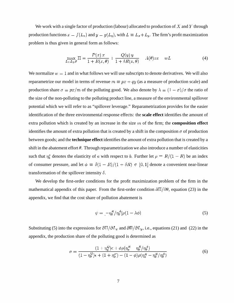
We work with a single factor of production (labour) allocated to production of � and � through

production functions � �ed 'fhg and � �"i 'fhj , with f � fXgk�lfhj . The firm’s profit maximization

problem is thus given in general form as follows:

Gnmpoq_r:s q?t�s I�u � / � ��v� ( �w)x! � < � ��y� 2?( �w)x! � @ ! ZO � �{zQf (4)

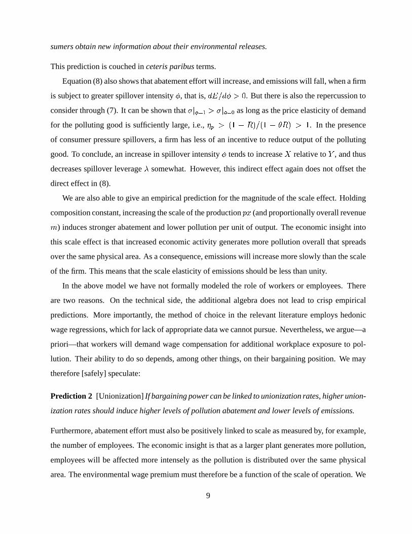
We normalize z � � and in what follows we will use subscripts to denote derivatives. We will also

reparametrize our model in terms of revenue | � .8� � ;p� (as a measure of production scale) and

production share } � .� � | of the polluting good. We also denote by ~ � ���� } � } the ratio of

the size of the non-polluting to the polluting product line, a measure of the environmental spillover

potential which we will refer to as “spillover leverage.” Reparametrization provides for the easier

identification of the three environmental response effects: the scale effect identifies the amount of

extra pollution which is created by an increase in the size | of the firm; the composition effect

identifies the amount of extra pollution that is created by a shift in the composition } of production

between goods; and the technique effect identifies the amount of extra pollution that is created by a

shift in the abatement effort ! . Through reparametrization we also introduce a number of elasticities

such that T+�� denotes the elasticity of A with respect to � . Further let � � ( �8��>� ( be an index

of consumer pressure, and let � � 2 ���� ( �K�Q� 2p( 3�5��8) ��9 denote a convenient near-linear

transformation of the spillover intensity 2 .We develop the first-order conditions for the profit maximization problem of the firm in the

mathematical appendix of this paper. From the first-order condition � u � �k! , equation (23) in the

appendix, we find that the cost share of pollution abatement is

[ � 5 � T+�I � T UI 9 � ��v� ~�� (5)

Substituting (5) into the expressions for � u � � fXg and � u � � fhj , i.e., equations (21) and (22) in the

appendix, the production share of the polluting good is determined as

} � ��v� T8�j �� � ��� T �g � T �I � T UI K�v� T �j Z� �eK�y� T+�g ����1� � � T �g � T �I � T UI (6)

7

Further making use of the explicit functional forms for

@and ( , we obtain

~ � K�v� T �g ����v� ! �K�y� T �j �� �e��v� ! ��� (7)

For (5) we obtain [ � !?� K�h� ~�� , and if we assume that �$��( ��� K�X� ! �O .� for small values

of ( , we can obtain an explicit solution for the optimal abatement level ! similar to (3):

! � �1�a� A� K��� ~�� .8� (8)

Equations (7) and (8) illustrate the interaction between the technique effect (linked to ! ) and the

composition effect (linked to ~ ). From equation (8) it is apparent that an increase in consumer

pressure spillover potential ~ increases abatement effort ! . But there is also a repercussion effect.

Equation (7) implies that an increase in ! lowers ~ (or equivalently, increases } ). This means that

the firm is able to shift shift some production back from the non-polluting to the polluting sector.

This indirect effect partially offsets the direct effect. Which effect will prevail?

We are interested in the overall effect on emissions & � K��� ! �O � which depends on all three

effects: scale, composition, and technique. Since we cannot solve equation system (7)-(8) explicitly

due to the non-linear nature of the expressions, we employ implicit function calculus to determine

the sign of the effect from the Jacobi matrix of the first-order conditions. The resulting expression

is too complex to sign unambiguously, but we obtain convincing results from calculating numeric

solutions for a wide range of typical parametrizations. We find that overall emissions decrease with

(a) a decrease in the abatement cost parameter A ; (b) a decrease in the pollution intensity parameterO ; (c) an increase in the consumer pressure intensity�; (d) a decrease in the demand elasticity of

the polluting good; and (e) an increase in the demand elasticity of the non-polluting good. Finally,

we find that the direct effect in (8) dominates: holding scale constant, greater spillover leverage ~triggers stronger pollution abatement and in turn lower emissions ( � &4� ��~�#�� ). We restate this

important result in an empirical prediction:

Prediction 1 [Spillover Leverage] Given two firms of equal size of polluting production line � ,

the firm subject to larger spillover leverage ~ will have lower emissions & . More generally, a more

diversified firm will increase pollution abatement relative to another less diversified firm when con-

8

sumers obtain new information about their environmental releases.

This prediction is couched in ceteris paribus terms.

Equation (8) also shows that abatement effort will increase, and emissions will fall, when a firm

is subject to greater spillover intensity � , that is, � &4� ��� B � . But there is also the repercussion to

consider through (7). It can be shown that }y� ����L B }y� ���� as long as the price elasticity of demand

for the polluting good is sufficiently large, i.e., T�� B ��-� ( �K�$� !_( B � . In the presence

of consumer pressure spillovers, a firm has less of an incentive to reduce output of the polluting

good. To conclude, an increase in spillover intensity � tends to increase � relative to � , and thus

decreases spillover leverage ~ somewhat. However, this indirect effect again does not offset the

direct effect in (8).

We are also able to give an empirical prediction for the magnitude of the scale effect. Holding

composition constant, increasing the scale of the production .� (and proportionally overall revenue| ) induces stronger abatement and lower pollution per unit of output. The economic insight into

this scale effect is that increased economic activity generates more pollution overall that spreads

over the same physical area. As a consequence, emissions will increase more slowly than the scale

of the firm. This means that the scale elasticity of emissions should be less than unity.

In the above model we have not formally modeled the role of workers or employees. There

are two reasons. On the technical side, the additional algebra does not lead to crisp empirical

predictions. More importantly, the method of choice in the relevant literature employs hedonic

wage regressions, which for lack of appropriate data we cannot pursue. Nevertheless, we argue—a

priori—that workers will demand wage compensation for additional workplace exposure to pol-

lution. Their ability to do so depends, among other things, on their bargaining position. We may

therefore [safely] speculate:

Prediction 2 [Unionization] If bargaining power can be linked to unionization rates, higher union-

ization rates should induce higher levels of pollution abatement and lower levels of emissions.

Furthermore, abatement effort must also be positively linked to scale as measured by, for example,

the number of employees. The economic insight is that as a larger plant generates more pollution,

employees will be affected more intensely as the pollution is distributed over the same physical

area. The environmental wage premium must therefore be a function of the scale of operation. We

9

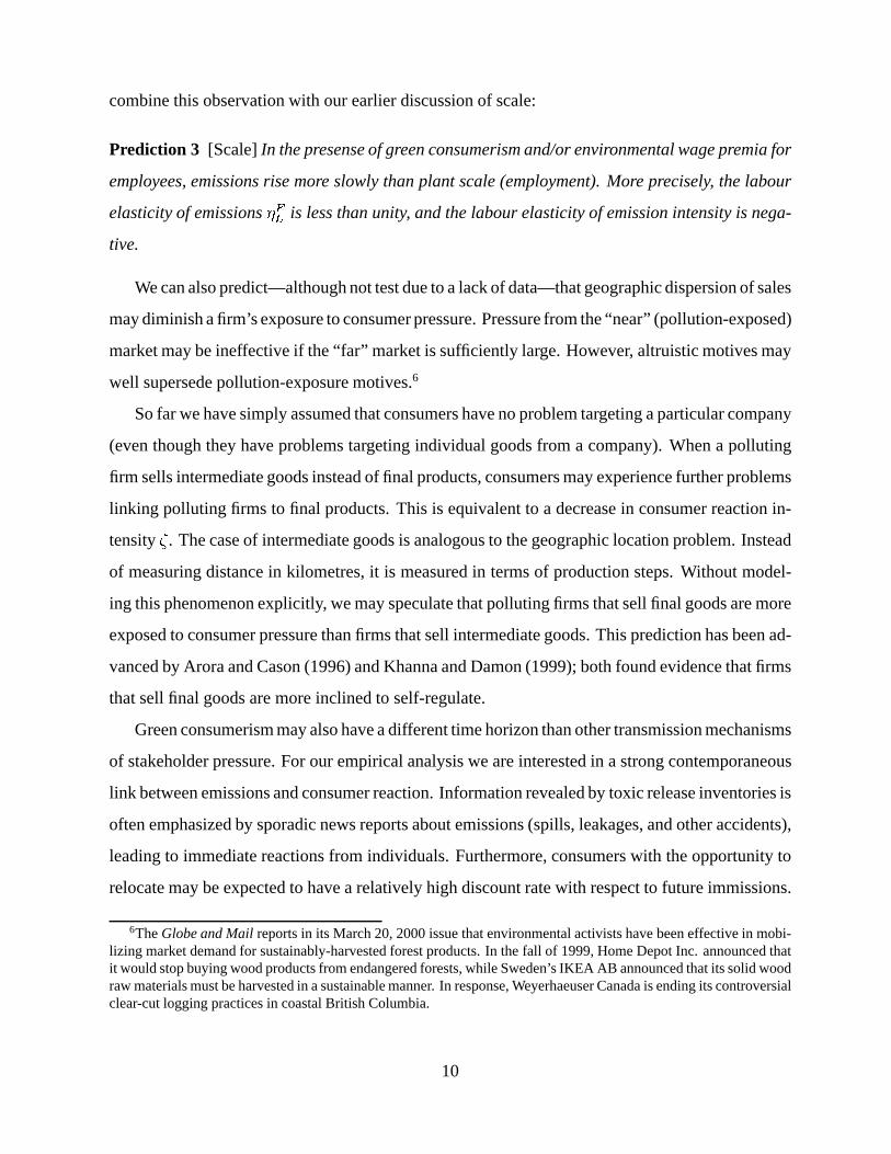
combine this observation with our earlier discussion of scale:

Prediction 3 [Scale] In the presense of green consumerism and/or environmental wage premia for

employees, emissions rise more slowly than plant scale (employment). More precisely, the labour

elasticity of emissions T��q is less than unity, and the labour elasticity of emission intensity is nega-

tive.

We can also predict—although not test due to a lack of data—that geographic dispersion of sales

may diminish a firm’s exposure to consumer pressure. Pressure from the “near” (pollution-exposed)

market may be ineffective if the “far” market is sufficiently large. However, altruistic motives may

well supersede pollution-exposure motives.6

So far we have simply assumed that consumers have no problem targeting a particular company

(even though they have problems targeting individual goods from a company). When a polluting

firm sells intermediate goods instead of final products, consumers may experience further problems

linking polluting firms to final products. This is equivalent to a decrease in consumer reaction in-

tensity�. The case of intermediate goods is analogous to the geographic location problem. Instead

of measuring distance in kilometres, it is measured in terms of production steps. Without model-

ing this phenomenon explicitly, we may speculate that polluting firms that sell final goods are more

exposed to consumer pressure than firms that sell intermediate goods. This prediction has been ad-

vanced by Arora and Cason (1996) and Khanna and Damon (1999); both found evidence that firms

that sell final goods are more inclined to self-regulate.

Green consumerism may also have a different time horizon than other transmission mechanisms

of stakeholder pressure. For our empirical analysis we are interested in a strong contemporaneous

link between emissions and consumer reaction. Information revealed by toxic release inventories is

often emphasized by sporadic news reports about emissions (spills, leakages, and other accidents),

leading to immediate reactions from individuals. Furthermore, consumers with the opportunity to

relocate may be expected to have a relatively high discount rate with respect to future immissions.

6The Globe and Mail reports in its March 20, 2000 issue that environmental activists have been effective in mobi-lizing market demand for sustainably-harvested forest products. In the fall of 1999, Home Depot Inc. announced thatit would stop buying wood products from endangered forests, while Sweden’s IKEA AB announced that its solid woodraw materials must be harvested in a sustainable manner. In response, Weyerhaeuser Canada is ending its controversialclear-cut logging practices in coastal British Columbia.

10

3 Toxicity of Pollutants

As the toxicity of chemicals varies greatly, health or environmental risks may not be proportional

to the weight of total discharges reported in toxic release inventories. If consumers were to base

their reaction merely on the weight of total discharges without adjusting for the toxicity of different

substances,there is a chance that risks could actually increase over time if firms substitute low vol-

ume, high toxicity substances for high volume, low toxicity ones. Our empirical analysis rests on

the assumption that consumers are able to make decisions based on information about the toxicity

of pollutants. Because of this additional step of processing information, our empirical analysis also

amounts to a stricter test for the presence of green consumerism compared to an analysis based on

emission aggregates unadjusted for toxicity. In technical terms, our parameter�

reflects an aggre-

gation of (actual or perceived) immissions, and thus reflects consumers’ opinions about the relative

importance of the pollutants.

Following the example of Hettige et al. (1992) and Horvath et al. (1995), and more recently

Shapiro (1999), we have tried to take into account the varying toxicity of NPRI substances. Like

Shapiro (1999), we are using the EPA Chronic Human Health Indicator (CHHI) for the purpose of

aggregating pollutants. The CHHI provides risk-related comparisons of chemical releases to var-

ious environmental media.7 An important advantage of the CHHI data is that EPA has developed

separate toxicity scores depending on whether exposure occurs via oral intake or inhalation. We

have employed inhalation scores for releases to air, and oral toxicity scores for all other releases.8

CHHI scores are based only on chronic effects and do not consider acute effects of exposure. How-

ever, this is arguably more appropriate in light of the low level exposures resulting from most en-

vironmental releases. CHHI indicators do not address multiple effects, effects of concurrent ex-

posures to multiple substances, nor environmental impacts other than human health.9 Our empir-

7For details about the CHHI please see the EPA’s web site at http://www.epa.gov/opptintr/env ind/chgtox.htm. Theearlier studies by Hettige et al. (1992) and Horvath et al. (1995) rely on threshold limit values (TLVs) adopted by theAmerican Conference of Governmental Industrial Hygienists, but this approach has several limitations. TLVs are de-signed to reflect the toxicity of airborne substances only, and the same toxicity rankings may not apply to other formsof exposure. Another drawback is that TLVs are developed for occupational settings, where exposures to toxic sub-stances tend to be high relative to ambient environmental exposures. The same toxicity rankings may not hold at lowerexposure levels.

8This assumes that the ultimate source of human exposure from land-based disposal techniques, including landfills,land-farming, and underground injection will be via surface or ground water contamination.

9Coverage of toxins by the TLV (see previous footnote) and CHHI measures is incomplete, but we can account for

11

ical analysis is based primarily on the CHHIs, but, following Hettige et al. (1992) and Horvath et

al. (1995), we have also used TLVs to check for robustness of our results. Due to space limitation,

we do not report the detailed results using TLVs, but make them available upon request. To interpret

our numbers, note that the CHHI adjustment expresses pollution in “methanol units.”

Environmental risk has (at least) two dimensions. We address toxicity, but exposure (which

is related to factors such as longevity of the pollutant, efficacy of treatment in the case of off-site

transfers, and degree of containment in storage) is not covered by our adjustment factors. This is a

serious caveat that we acknowledge but—for lack of data—cannot improve upon.

4 Data Preview

Canada’s NPRI now contains six years of data for the period 1993-98, covering roughly 2,400 facil-

ities. Facilities below a certain size (i.e., those with fewer than 10 employees that do not produce or

use NPRI substances in quantities greater than 10 tons, and those in certain exempt categories, such

as educational institutions) are not required to report. According to Olewiler and Dawson (1998),

of the roughly 32,000 manufacturing establishments identified by Statistics Canada, only about 4%

(now: 7%) report to NPRI.

Although facilities are required to report discharges on 176 substances, to date reports have been

received for only about 135 substances, with an average between 3 and 4 substance reports per fa-

cility each year. NPRI focuses on “toxic” substances, and thus does not include many traditional

pollutants, such as greenhouse gases, particulates released to air, or suspended solid to water. These

excluded substances undoubtedly present significant risks to health and the environment, and one

thus cannot conclude that trends in NPRI discharges tell the full story. Moreover, because the focus

of NPRI is “toxic” substances released in significant quantities, the inventory excludes both high

volume, low toxicity pollutants (such as the traditional pollutants noted above), as well as highly

toxic substances, such as dioxins, released in small quantities (referred to by Environment Canada

as ”micropollutants”). However, since the focus of this paper is on the impact of information dis-

semination as a policy instrument, and inventories of criteria and micro-pollutants are not readily

over 90% of the raw weight of pollutants by either method. One potential bias is with respect to nitrate; the CHHI doesnot provide both oral and inhalation scores.

12

available to the public, the focus on NPRI data alone is justified.

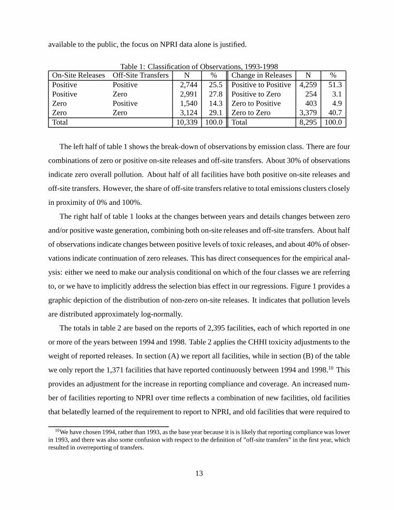
Table 1: Classification of Observations, 1993-1998On-Site Releases Off-Site Transfers N % Change in Releases N %Positive Positive 2,744 25.5 Positive to Positive 4,259 51.3Positive Zero 2,991 27.8 Positive to Zero 254 3.1Zero Positive 1,540 14.3 Zero to Positive 403 4.9Zero Zero 3,124 29.1 Zero to Zero 3,379 40.7Total 10,339 100.0 Total 8,295 100.0

The left half of table 1 shows the break-down of observations by emission class. There are four

combinations of zero or positive on-site releases and off-site transfers. About 30% of observations

indicate zero overall pollution. About half of all facilities have both positive on-site releases and

off-site transfers. However, the share of off-site transfers relative to total emissions clusters closely

in proximity of 0% and 100%.

The right half of table 1 looks at the changes between years and details changes between zero

and/or positive waste generation, combining both on-site releases and off-site transfers. About half

of observations indicate changes between positive levels of toxic releases, and about 40% of obser-

vations indicate continuation of zero releases. This has direct consequences for the empirical anal-

ysis: either we need to make our analysis conditional on which of the four classes we are referring

to, or we have to implicitly address the selection bias effect in our regressions. Figure 1 provides a

graphic depiction of the distribution of non-zero on-site releases. It indicates that pollution levels

are distributed approximately log-normally.

The totals in table 2 are based on the reports of 2,395 facilities, each of which reported in one

or more of the years between 1994 and 1998. Table 2 applies the CHHI toxicity adjustments to the

weight of reported releases. In section (A) we report all facilities, while in section (B) of the table

we only report the 1,371 facilities that have reported continuously between 1994 and 1998.10 This

provides an adjustment for the increase in reporting compliance and coverage. An increased num-

ber of facilities reporting to NPRI over time reflects a combination of new facilities, old facilities

that belatedly learned of the requirement to report to NPRI, and old facilities that were required to

10We have chosen 1994, rather than 1993, as the base year because it is is likely that reporting compliance was lowerin 1993, and there was also some confusion with respect to the definition of ”off-site transfers” in the first year, whichresulted in overreporting of transfers.

13

Figure 1: Distribution of Total On-Site Emissions

Log10 of Toxicity-Equivalent Total On-Site Emissions

Num

ber

of N

on-Z

ero

Obs

erva

tions

-6<-5

-5<-4

-4<-3

-3<-2

-2<-1

-1<0

0<1

1<2

2<3

3<4

4<5

5<6

0

100

200

300

400

500

600

700

800

900

1000

1100

1200

1300

1400

1500

report only after a change in NPRI reporting requirements in 1995. Inclusion of these older facili-

ties in Section (A) will tend to overstate increases in releases (and understate decreases). In Section

(B) we thus adjust for this coverage bias by only focusing on continuous reporters. However, it is

noteworthy that Section B excludes both increases in releases from facilities that began operations

during this period as well as decreases as a result of closure of older facilities.

The fact that reductions in on-site releases from 1994 to 1998 by all facilities reporting to NPRI

(-23%) exceed those by continuous reporters (-17%) suggests that reductions have been achieved

primarily through closure of facilities rather than reductions at continuing facilities. It is notewor-

thy that, during 1994-98, offsite transfers increased by more than 90% for continuing firms, and by

over 150% overall. As a result, total releases increased by about 36%. The release categories that

have seen large decreases are water and underground injection. The decrease in water pollution is

largely accounted for by the pulp and paper industry (CSIC 27), which was the the only industry that

faced new discharge regulations at the national level during this period, and which was also subject

to extensive reform of regulations and permits at the provincial level in the early 1990s (Harrison,

1996), as well as a single facility in Quebec, Kronos, that dramatically reduced its releases in re-

sponse to regulatory enforcement action by both the federal government and the province.

14

Table 2: Summary of Trends in On-Site Releases and Off-Site Transfers(A) All Facilities Reporting

%-Chg.Release Method 1994 1995 1996 1997 1998 1994-98Air 152,256 98,522 106,752 104,999 97,821 -35.8Water 16,587 8,498 6,318 3,751 2,970 -82.1Land 87,091 83,895 90,201 88,534 99,164 13.9Underground Injection 11,744 11,033 8,856 5,705 5,501 -53.2Total On-Site Release 267,678 201,948 212,127 202,990 205,457 -23.2Offsite Transfers 132,089 212,474 250,768 414,245 338,830 156.5Total Release 399,767 414,423 462,895 617,235 544,286 36.2

(B) Subset of continuous reporters 1994 through 1998%-Chg.

Release Method 1994 1995 1996 1997 1998 1994-98Air 98,212 96,357 103,611 101,156 92,077 -6.2Water 16,260 8,174 6,221 3,698 2,925 -82.0Land 87,023 83,822 84,868 83,201 75,784 -12.9Underground Injection 11,742 11,031 8,856 5,704 5,500 -53.2Total On-Site Release 213,236 199,385 203,555 193,760 176,286 -17.3Offsite Transfers 123,336 194,557 221,816 313,127 234,431 90.1Total Release 336,573 393,942 425,371 506,887 410,717 22.0

Note: Figures report tons of discharges adjusted for toxicity with the EPA Chronic HumanHealth Indicators

5 Empirical Results

Empirically testing the propositions derived in the theory section is a challenging task due to data

limitations as well as identification problems. We begin by defining our dependent variables.

Let facilities (plants) be denoted by indexd�� � )��H��)x�¡  for company ¢ � � )£���H)x¤ . Index ¥ denotes

time. Pollutants are indexed by . � � )��H��) / with toxicity ¦§�x¨ for release method © � � )£�H��)x( . Raw

emissions are denoted by &>ª  «��¨­¬ . In our regression, our dependent variables are calculated as

� ª  ®¬ � DH¯±° L²��³´ �µ�¶��L �µ¨K��L &Sª  «�x¨·¬²¦§��¨Z¸¹ (9)º � ª  ®¬ � � ª   s ¬ � � ª   s ¬¼»+½ �±¾ (10)¿ ª  ®¬ � � ª  ®¬ � DH¯±° L²� ²f�ª  ®¬ (11)

where ¾ is the year distance to the latest available prior observation. The log levels � ª  ®¬ are depicted

in figure 1, indicating that the distribution is approximately log-normal.¿ ª  ®¬ is the log of pollution

15

intensity with respect to the number of employees at a given facility.11 Our dependent variables

seek to proxy abatement behaviour by focusing on the level and change in pollution as well as the

intensity of pollution.

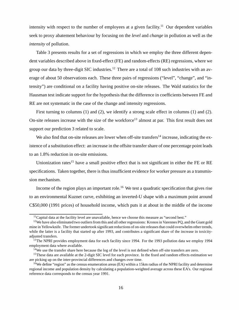
Table 3 presents results for a set of regressions in which we employ the three different depen-

dent variables described above in fixed-effect (FE) and random-effects (RE) regressions, where we

group our data by three-digit SIC industries.12 There are a total of 108 such industries with an av-

erage of about 50 observations each. These three pairs of regressions (“level”, “change”, and “in-

tensity”) are conditional on a facility having positive on-site releases. The Wald statistics for the

Hausman test indicate support for the hypothesis that the difference in coefficients between FE and

RE are not systematic in the case of the change and intensity regressions.

First turning to columns (1) and (2), we identify a strong scale effect in columns (1) and (2).

On-site releases increase with the size of the workforce13 almost at par. This first result does not

support our prediction 3 related to scale.

We also find that on-site releases are lower when off-site transfers14 increase, indicating the ex-

istence of a substitution effect: an increase in the offsite transfer share of one percentage point leads

to an 1.8% reduction in on-site emissions.

Unionization rates15 have a small positive effect that is not significant in either the FE or RE

specifications. Taken together, there is thus insufficient evidence for worker pressure as a transmis-

sion mechanism.

Income of the region plays an important role.16 We test a quadratic specification that gives rise

to an environmental Kuznet curve, exhibiting an inverted-U shape with a maximum point around

C$50,000 (1991 prices) of household income, which puts it at about in the middle of the income

11Capital data at the facility level are unavailable, hence we choose this measure as “second best.”12We have also eliminated two outliers from this and all other regressions: Kronos in Varennes PQ, and the Giant gold

mine in Yellowknife. The former undertook significant reductions of on-site releases that could overwhelm other trends,while the latter is a facility that started up after 1993, and contributes a significant share of the increase in toxicity-adjusted transfers.

13The NPRI provides employment data for each facility since 1994. For the 1993 pollution data we employ 1994employment data where available.

14We use the transfer share here because the log of the level is not defined when off-site transfers are zero.15These data are available at the 2-digit SIC level for each province. In the fixed and random effects estimation we

are picking up on the inter-provincial differences and changes over time.16We define “region” as the census enumeration areas (EA) within a 15km radius of the NPRI facility and determine

regional income and population density by calculating a population-weighted average across these EA’s. Our regionalreference data corresponds to the census year 1991.

16

Table 3: Basic On-Site Releases RegressionsDependent Variable À_ÁVÂFà Ä�À±ÁVÂFà ÅkÁVÂFÃEstimation Method F.E. R.E. F.E. R.E. F.E. R.E.Variable / Column (1) (2) (3) (4) (5) (6)

Intercept ÆwÇpÈÊÉ�Ë¶Ë Â ÆwÇpÈ Ì£ÉxÌ Â ÆXÍ:È Ç:Ì:Î¶Ï ÆXÍ:È Ç�Ð¶Ð¶Ï ÆXÍ¶È ÇÑÍ:Í�Ï ÆXͶÈÊÎ�Ë:Ò:Ï( ÓÑÈ Ë�É ) ( ÉWÈÔÍ�Ì ) ( ÇpÈ Ò�Î ) ( ÎÑÈ Ì£É ) ( ÎÑÈ ËpÍ ) ( ÎÑÈÊÉ:É )

Log Õ×Ö of employees at facility ÒpÈ Ì:ÌÑÍ Â ÒÑÈ Ì�ɶР ÆwÒpÈ Ò:Ë�Ø�Ù ÆwÒpÈ Ò:˶Ó:Ù ÆwÒÑÈÚÍZÒ¶Ø�Ï ÆwÒÑÈÚÍZÒ�жÏ( Î:ÎWÈ Ë¶Ë ) ( ζÇÑÈ Ò:Ð ) ( ÎÑÈ Î¶Ì ) ( ÎÑÈ Ø�Ó ) ( ÎÑÈ Ë:Ç ) ( ÎÑÈ Ì:Ë )

Change in Employment (log-diff) ÒÑÈ Ó�أΠ ÒÑÈ ÓÑÍ�Ò Â( Ø?È Î�Ø ) ( Ø?È Ò:Ç )

% of Off-site Transfers ÆwÒpÈ Ò:Ò¶Ì Â ÆwÒpÈ Ò:Ò¶Ì Â ÆwÒpÈ Ò:Ò:Ð Â ÆwÒpÈ Ò:Ò:Ð Â ÆwÒÑÈ Ò¶Ò�Ð Â ÆwÒÑÈ Ò¶Ò�Ð Â( Í�ÇÑÈ ÌÑÍ ) ( Í�ÇÑÈ Ì¶Ç ) ( ÌpÈ Î¶Ó ) ( ÌpÈ Ø�Ò ) ( ÌpÈ ØWÉ ) ( ÌpÈ Ó:Ò )

Lagged pollution intensity ÅkÁVÂ'Û Ã¼Ü Õ ÆwÒpÈ Ð¶Ç¶Ì Â ÆwÒpÈ Ð¶ÇÑÍ Â ÒÑÈ Ø�ÐÑÍ Â ÒÑÈ Ø�Ð¶Ì Â( Ó�ÐWÈ Ø�Î ) ( Ó:ÐÑÈÔÍ�Ò ) ( ÐxØ?ÈÔÍ�Ì ) ( жÐÑÈ Ó�Ð )

Unionization Rate in Ind./Prov. ÆwÒpÈ Ò:ÒÑÍ ÆwÒpÈ Ò:ÒÑÍ ÒÑÈ Ò¶ÒpÍ ÒÑÈ Ò¶Ò:Ò ÒÑÈ Ò¶ÒpÍ ÒÑÈ Ò¶Ò:Ò( ÒÑÈ Ç¶Ó ) ( ÒpÈ Ø£Ð ) ( ÒpÈ Ø£Î ) ( ÒpÈÔÍ�Ò ) ( ÒpÈ Ð¶Ç ) ( ÒpÈ Î¶Ó )

Income of Region ($10k) ÒpÈ Ó:ǶÌ:Ï ÒÑÈ Ó¶Ó¶Ø�Ï ÒÑÈÊζÎ:Ð ÒÑÈÊζÎ�Ø ÒÑÈÚÍZÌ:Ì ÒÑÈÚÍZÌ:Ë( ÎWÈ Ì¶Ó ) ( ÇpÈÔÍ�Ò ) ( Í:È Î¶Ó ) ( Í:È Î¶Ó ) ( Í:ÈÔÍ�Ò ) ( Í:ÈÔÍ�Ò )

Income squared ÆwÒpÈ Ò:Ó�Ø�Ï ÆwÒpÈ Ò:Ó¶Ó Â ÆwÒpÈ Ò�ÎxØ ÆwÒpÈ Ò�Î�Ç ÆwÒÑÈ Ò:ÎÑÍ ÆwÒÑÈ Ò:ÎÑÍ( ÇÑÈ Ò�É ) ( ÇpÈÔÍ�Ì ) ( Í:È Ç:Ó ) ( Í:È Ç£É ) ( Í:ÈÔÍ�Ë ) ( Í:ÈÔÍ�Ì )

Log Õ×Ö Population Density ÆwÒpÈÔÍ�Ç:Î Â ÆwÒpÈÔÍ�ÇÑÍ Â ÆwÒpÈ Ò¶Ø£É ÆwÒpÈ Ò�Ð�Ç:Ù ÆwÒÑÈ Ò:Ð:ж٠ÆwÒÑÈ Ò¶ÓpÍ�Ù( ØpÈ Ç¶Ò ) ( Ø?È Ç:Ó ) ( Í:È Ë¶Ø ) ( ÎÑÈÔÍVÎ ) ( ÎÑÈÔÍVÐ ) ( ÎÑÈ Ø£Î )

Time Trend ÆwÒpÈ ÒpÍZÒ ÆwÒpÈ Ò:Ò¶Ì ÆwÒpÈ Ò:Ó:Î Â ÆwÒpÈ Ò�Ð�Ë Â ÆwÒÑÈ Ò:Ð�É Â ÆwÒÑÈ Ò:Ð¶Ç Â( ÒÑÈ Ë:Î ) ( ÒpÈÊÉ�Ç ) ( ÐÑÈ Ç:Ò ) ( Ø?È Ì¶Ø ) ( Ø?È Ë¶Ø ) ( Ø?È Ø�Ë )

Observations 5180 5180 4252 4252 4254 4254Groups 108 108 106 106 106 106Adj./Pseudo ÝhÞ 0.2046 0.2047 0.4372 0.4373 0.5096 0.5094Hausman Test / Wald ß8Þ (df) 7.41 52.3 54.49

Note: Dependent variables are on-site releases ( À ¼à�à ), changes in on-site releases( ÄvÀ ¼àÔà ) and pollution intensity( Š¼àÔà ), all adjusted for toxicity using CHHI measures. Estimation methods are fixed effects (F.E.) and randomeffects (R.E.) based on 3-digit Canadian-SIC industry groups. Observations where on-site releases are zerowere excluded from this set of regressions. T-statistics (without sign) are given in parentheses. Significance atthe 95%, 99%, and 99.9% levels are indicated with the superscripts a, b and c.

range of our data. Population density also has a negative effect on emission levels. Polluting facil-

ities apparently avoid high-density urban areas. A doubling of population density leads to a 12%

reduction in on-site releases. In the case of resource-based industries such as mining and pulp man-

ufactured, location choice is strongly influenced by geographic proximity to the resource. The pre-

dominance of polluting facilities in rural Canada may thus reflect geographic as well as economic

motives.

In columns (3) and (4) we turn to an analysis ofº � ª  ®¬ , the change in on-site releases from period

to period. In this regression we introduce the pollution intensity (lagged by one period) as a new

regressor, as well as the change in employment (likeº � ª  ®¬ this is expressed as the difference of

17

logs). It turns out that pollution intensity is the single most important predictor of changes in on-

site releases. Pollution-intensive firms have reduced their emissions by more than those that are

less pollution-intensive. At the same time, large facilities also make greater progress in reducing

on-site releases than smaller facilities, and pollution changes slower than employment (scale).

The findings relating to the size of the plant are consistent with stakeholder pressure, since one

would expect consumers and workers to put the most pressure on the most pollution-intensive and

more recognizable facilities. However, they could also reflect a similar or anticipated response by

regulators. Similar to the approach for the levels regression, we estimate a Kuznet curve and a

population density effect. Neither turns out to be of significance for the rate of change in emissions.

This suggests that, although pollution was correlated with income and population density when the

NPRI was launched, and continues to be since NPRI, the dissemination of additional information

via NPRI does not appear to have had a greater or lesser effect in communities that vary along these

dimensions. The unionization rate is again insignificant as an explanatory variable.

The last two columns in table 3 report results for our pollution intensity regressions where again

we include lagged pollution intensity as a regressor. The interpretation of the results in columns (5)

and (6) is somewhat similar to columns (3) and (4). We again find that larger firms reduce pollu-

tion intensity more. We take this as further evidence of prediction 3.17 Unionization rates have no

discernible effect on emissions. Regressions (5) and (6) identify the environmental Kuznet curve

effect only weakly, in part due to the fact that our income variable does not have time variation.

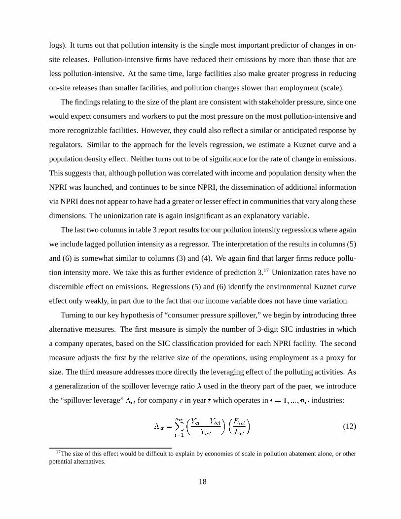
Turning to our key hypothesis of “consumer pressure spillover,” we begin by introducing three

alternative measures. The first measure is simply the number of 3-digit SIC industries in which

a company operates, based on the SIC classification provided for each NPRI facility. The second

measure adjusts the first by the relative size of the operations, using employment as a proxy for

size. The third measure addresses more directly the leveraging effect of the polluting activities. As

a generalization of the spillover leverage ratio ~ used in the theory part of the paer, we introduce

the “spillover leverage” áy ®¬ for company ¢ in year ¥ which operates in â � � )£���H��) �  ®¬ industries:

áv ®¬ �äã�å¼æµç ��Léè �k ®¬ � �ç  ®¬� ç  ®¬ ê è &

ç  ®¬&  ®¬+ê (12)

17The size of this effect would be difficult to explain by economies of scale in pollution abatement alone, or otherpotential alternatives.

18

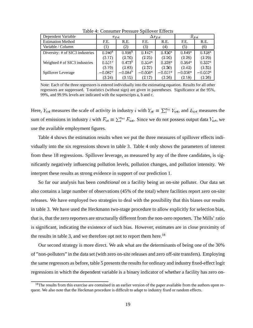
Table 4: Consumer Pressure Spillover EffectsDependent Variable À_ÁVÂFÃ ÄvÀ_ÁVÂFÃ ÅkÁVÂFÃEstimation Method F.E. R.E. F.E. R.E. F.E. R.E.Variable / Column (1) (2) (3) (4) (5) (6)

Diversity: # of SIC3 industries ÆwÒpÈ Î�Ø:Ò�Ï ÆwÒpÈÔÍ�̶Ë�Ï ÆwÒpÈÔÍZØ£É�Ù ÆwÒpÈÔÍ�ǶÓ:Ù ÆwÒpÈÔÍZØ:Ì:Ù ÆwÒpÈÔÍ�ǶË:Ù( ÇÑÈÚÍVÉ ) ( ÎWÈ7ÉxÓ ) ( ÎWÈÊζР) ( ÎWÈÊÎ�Ó ) ( ÎÑÈ Î¶Ë ) ( ÎÑÈ Î¶Ì )

Weighted # of SIC3 industries ÆwÒpÈ Ð:ÐWÍ Â ÆwÒpÈ ØWÉxÇ�Ï ÆwÒpÈ Ç�ÐxØ�Ù ÆwÒpÈ Ç�Î�Ë:Ù ÆwÒpÈ Ç:Ó�Ø�Ù ÆwÒpÈ Ç:Ç�É�Ù( ÇÑÈÚÍZÌ ) ( ÎWÈ Ë¶Ç ) ( ÎWÈ Ç�É ) ( ÎWÈ Ç¶Ò ) ( ÎÑÈ Ø£Î ) ( ÎÑÈ Ç�Ð )

Spillover Leverage ÆwÒpÈ Ò:Ë�É Â ÆwÒpÈ Ò:Ë�Ø£Ï ÆwÒpÈ Ò�Ð�Ò:Ù ÆwÒpÈ Ò�ÐWÍ�Ù ÆwÒpÈ Ò�Ð�Ò:Ù ÆwÒpÈ Ò�жζÙ( ÇÑÈÊÎxØ ) ( ÇÑÈÚÍ�Ð ) ( ÎWÈÚÍVÉ ) ( ÎWÈÊÎ�Ó ) ( ÎÑÈÔÍ�Ë ) ( ÎÑÈ Î¶Ó )

Note: Each of the three regressors is entered individually into the estimating equation. Results for all otherregressors are suppressed. T-statistics (without sign) are given in parentheses. Significance at the 95%,99%, and 99.9% levels are indicated with the superscripts a, b and c.

Here, � ç  ×¬ measures the scale of activity in industry â with �� ®¬ �0ë ã:å¼æç � ç  ®¬ , and & ç  ®¬ measures the

sum of emissions in industry â with &  ×¬ � ë ã�å¼æç & ç  ×¬ . Since we do not possess output data � ç  ×¬ , we

use the available employment figures.

Table 4 shows the estimation results when we put the three measures of spillover effects indi-

vidually into the six regressions shown in table 3. Table 4 only shows the parameters of interest

from these 18 regressions. Spillover leverage, as measured by any of the three candidates, is sig-

nificantly negatively influencing pollution levels, pollution changes, and pollution intensity. We

interpret these results as strong evidence in support of our prediction 1.

So far our analysis has been conditional on a facility being an on-site polluter. Our data set

also contains a large number of observations (45% of the total) where facilities report zero on-site

releases. We have employed two strategies to deal with the possibility that this biases our results

in table 3. We have used the Heckmann two-stage procedure to allow explicitly for selection bias,

that is, that the zero reporters are structurally different from the non-zero reporters. The Mills’ ratio

is significant, indicating the existence of such bias. However, estimates are in close proximity of

the results in table 3, and we therefore opt not to report them here.18

Our second strategy is more direct. We ask what are the determinants of being one of the 30%

of ”non-polluters” in the data set (with zero on-site releases and zero off-site transfers). Employing

the same regressors as before, table 5 presents the results for ordinary and industry fixed-effect logit

regressions in which the dependent variable is a binary indicator of whether a facility has zero on-

18The results from this exercise are contained in an earlier version of the paper available from the authors upon re-quest. We also note that the Heckman procedure is difficult to adapt to industry fixed or random effects.

19

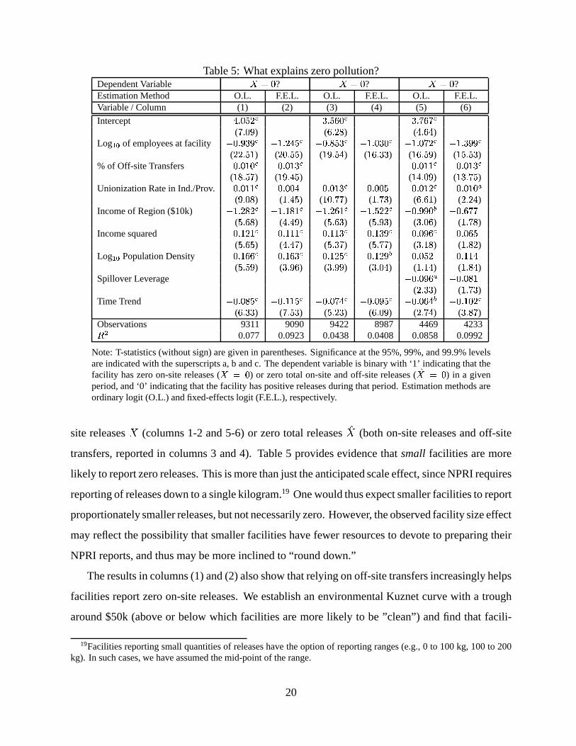
Table 5: What explains zero pollution?Dependent Variable ì"ílÒ ? îì"ílÒ ? ì�í§Ò ?Estimation Method O.L. F.E.L. O.L. F.E.L. O.L. F.E.L.Variable / Column (1) (2) (3) (4) (5) (6)

Intercept ØpÈ Ò:жΠ ÇpÈ Ð¶Ó¶Ò Â ÇpÈÊÉ�Ó�É Â( É£È Ò¶Ì ) ( ÓÑÈÊÎ�Ë ) ( ØpÈ Ó�Ø )

Log Õ®Ö of employees at facility ÆwÒÑÈ Ì¶Ç¶Ì Â ÆXͶÈÊÎxØ�Ð Â ÆwÒÑÈ Ë:Ð�Ç Â ÆXÍ¶È Ò¶Ç¶Ò Â ÆXÍ:È Ò£É�Î Â ÆXÍ:È Ç:Ì¶Ì Â( ζÎWÈÊÐWÍ ) ( Î�ÒÑÈÊжР) ( ÍZÌÑÈÊÐxØ ) ( ÍZÓÑÈ Ç¶Ç ) ( Í�ÓÑÈÊÐ�Ì ) ( ÍVÐWÈÊÐ�Ç )

% of Off-site Transfers ÒÑÈ ÒÑÍZÒ Â ÒÑÈ ÒÑÍZÇ Â ÒpÈ ÒpÍ¶Í Â ÒpÈ ÒpÍZÇ Â( ÍZËÑÈÊÐ:É ) ( ÍZÌÑÈ Ø�Ð ) ( ÍZØpÈ Ò¶Ì ) ( Í�ÇÑÈ7É�Ð )

Unionization Rate in Ind./Prov. ÒÑÈ ÒÑÍ¶Í Â ÒÑÈ Ò¶Ò�Ø ÒpÈ ÒpÍZÇ Â ÒpÈ Ò:Ò:Ð ÒpÈ ÒpÍ�Î Â ÒpÈ ÒpÍZÒ�Ù( ÌÑÈ Ò¶Ë ) ( Í¶È Ø�Ð ) ( ÍZÒÑÈ7É¶É ) ( ͶÈ7ÉxÇ ) ( ÓÑÈ ÓÑÍ ) ( ÎWÈÊÎxØ )

Income of Region ($10k) ÆXͶÈÊÎ�Ë:Î Â ÆXͶÈÚÍZËÑÍ Â ÆXͶÈÊÎ�ÓÑÍ Â ÆXͶÈÊжζΠ ÆwÒpÈ Ì:̶Ò�Ï ÆwÒpÈ Ó£É¶É( ÐWÈ Ó¶Ë ) ( ØpÈ Ø:Ì ) ( ÐWÈ Ó¶Ç ) ( ÐWÈ Ì¶Ç ) ( ÇÑÈ Ò¶Ó ) ( ͶÈ7ÉxË )

Income squared ÒÑÈÚÍ�ÎWÍ Â ÒÑÈÚÍ¶Í¶Í Â ÒpÈÔÍ:ÍZÇ Â ÒpÈÔÍ�Ç¶Ì Â ÒpÈ Ò:Ì¶Ó Â ÒpÈ Ò:Ó:Ð( ÐWÈ Ó:Ð ) ( ØpÈ Ø£É ) ( ÐWÈ Ç�É ) ( ÐWÈ7É¶É ) ( ÇÑÈÚÍZË ) ( Í¶È Ë:Î )

Log Õ®Ö Population Density ÒÑÈÚÍZÓ¶Ó Â ÒÑÈÚÍZÓ¶Ç Â ÒpÈÔÍVζР ÒpÈÔÍVÎ�Ì�Ï ÒpÈ Ò�жΠÒpÈÔÍ:Í�Ø( ÐWÈÊÐ�Ì ) ( ÇÑÈ Ì¶Ó ) ( ÇÑÈ Ì¶Ì ) ( ÇÑÈ Ò�Ø ) ( ͶÈÚÍ�Ø ) ( Í¶È Ë�Ø )

Spillover Leverage ÆwÒpÈ Ò:̶Ó�Ù ÆwÒpÈ Ò:ËÑÍ( ÎWÈ Ç¶Ç ) ( ͶÈ7ÉxÇ )

Time Trend ÆwÒÑÈ Ò¶Ë:Ð Â ÆwÒÑÈÚͶÍ�Ð Â ÆwÒÑÈ Ò�ÉVØ Â ÆwÒÑÈ Ò¶Ì:Ð Â ÆwÒpÈ Ò:Ó�Ø£Ï ÆwÒpÈÔÍ�Ò:Î Â( ÓÑÈ Ç¶Ç ) ( É£ÈÊÐ�Ç ) ( ÐWÈÊÎ�Ç ) ( ÓÑÈ Ò¶Ì ) ( ÎWÈ7ÉVØ ) ( ÇÑÈ Ë�É )

Observations 9311 9090 9422 8987 4469 4233Ý Þ 0.077 0.0923 0.0438 0.0408 0.0858 0.0992

Note: T-statistics (without sign) are given in parentheses. Significance at the 95%, 99%, and 99.9% levelsare indicated with the superscripts a, b and c. The dependent variable is binary with ‘1’ indicating that thefacility has zero on-site releases ( ìïícÒ ) or zero total on-site and off-site releases ( îìðí�Ò ) in a givenperiod, and ‘0’ indicating that the facility has positive releases during that period. Estimation methods areordinary logit (O.L.) and fixed-effects logit (F.E.L.), respectively.

site releases � (columns 1-2 and 5-6) or zero total releases ñ� (both on-site releases and off-site

transfers, reported in columns 3 and 4). Table 5 provides evidence that small facilities are more

likely to report zero releases. This is more than just the anticipated scale effect, since NPRI requires

reporting of releases down to a single kilogram.19 One would thus expect smaller facilities to report

proportionately smaller releases, but not necessarily zero. However, the observed facility size effect

may reflect the possibility that smaller facilities have fewer resources to devote to preparing their

NPRI reports, and thus may be more inclined to “round down.”

The results in columns (1) and (2) also show that relying on off-site transfers increasingly helps

facilities report zero on-site releases. We establish an environmental Kuznet curve with a trough

around $50k (above or below which facilities are more likely to be ”clean”) and find that facili-

19Facilities reporting small quantities of releases have the option of reporting ranges (e.g., 0 to 100 kg, 100 to 200kg). In such cases, we have assumed the mid-point of the range.

20

ties are more likely to report zero releases in densely populated areas. Noteworthy is that we also

find a consistent negative time trend that indicates facilities are becoming less likely to report zero

releases. This may perhaps be interpreted as a spurious result from increasing NPRI reporting com-

pliance. Finally, we observe in columns (5) and (6) that spillover leverage is associated with a de-

creased likelihood of reporting zero releases, but this result is only weakly statistically significant; it

may indeed be a result of the correlation between spillover leverage (company diversification) and

facility size (diversified firms tending to have larger facility sizes on average). The results in col-

umn (3) and (4) for total on-site and off-site indicate a smaller scale effect compared to columns (1)

and (2). This result is consistent with the presence of a substitution effect between on-site releases

and off-site transfers.

6 Caveats

In this paper we have focused our attention on green consumerism as a key mechanism for transmis-

sion of stakeholder pressure. We have ignored pressures from regulators, shareholders, and com-

petitors, and we have not addressed consumers’ and firms’ location choice explicitly. In particular,

residential relocation will significantly diminish the scope for green consumerism if (a) pollution

is locally concentrated, (b) transaction costs associated with mobility are low, and (c) commuting

costs are low.

A shortcoming in our econometric work is related to the lack of data on the degree to which com-

panies produce final or intermediate goods. Such data would allow us to construct a suitable dis-

tance metric for testing the hypothesis that companies closer to the final-goods market are more ex-

posed to consumer pressure than companies that produce intermediate goods. Available data from

Canada’s input-output matrix would in principle provide such a metric, but unfortunately it would

be absorbed by our industry-specific fixed effects.

Finally, we ignore the potential endogeneity of our key regressor: high emission levels may

be a reason that prevents companies from diversifying into other areas exactly because they fear

consumer pressure spillover effects. Even though this effect is a hypothetic possibility, it is likely

to be very small. A related practical problem is the choice of suitable instrumental variables at the

facility level, the search for which is limited by the NPRI data set.

21

7 Conclusions

In this paper we have set out to test the empirical relevance of “green consumerism” through a sim-

ple economic model that yields plausible predictions which we test empirically using 1993-98 panel

data from Canada’s National Pollutant Release Inventory. Our key findings are summarized below.ò We find evidence of green consumerism when we allow for the possibility that consumers tar-

get companies rather than products. Firms with polluting and non-polluting product lines may

thus be subject to an intra-firm inter-plant externality which magnifies the impact of green

consumerism. The size of the effect—as captured through three alternative measures—is sta-

tistically significant and practically relevant.ò Local characteristics such as income and population density have a significant impact on pol-

luting behaviour of facilities. Pollution is lower where the population is more dense, and firms

also appear to have responded to disclosure of their toxic releases by more aggressively re-

ducing their releases when they are located in more densely populated areas. We identify an

environmental Kuznet curve but do not find that facilities’ response to information disclosure

via NPRI is significantly correlated with community income.ò We establish the existence of a scale effect which is indicative of pressure from consumers

and/or workers, but we acknowledge the possibility of alternative explanations for this effect

such as greater regulatory pressure on larger firms or economies of scale in pollution abate-

ment.ò There is little support for the hypothesis that worker pressure is facilitated through collective

bargaining power as measured by rates of unionization.ò Smaller firms are more likely to report zero releases and are more likely to switch from report-

ing positive releases to reporting zero releases. However, we cannot rule out that our results

are biased due to reporting thresholds in the NPRI data.

Overall, we find that there is an encouraging positive trend in the on-site releases reported to

the Canadian National Pollutant Release Inventory when toxicity adjustments are applied. How-

ever, offsite transfers have dramatically increased even when taking into account reporting bias

from higher compliance and new facilities.

22

A Mathematical Appendix

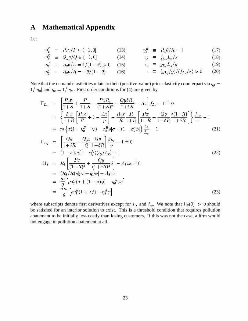
Let T �g � / g � � / 3 ��-� )x� 9 (13)T �j � < j � � < 3 K��� )V� 9 (14)T UI � @ Ix! � @ � ��8��1� ! B � (15)T+�I � (�Ix! � ( � � ! �8��1� ! (16)

T �g � ( g ! � ( � � (17)� g � d q r fhg?� � (18)� j � i q t fXj�� � (19)� � i q t � � �8 d q r � � B � (20)

Note that the demand elasticities relate to their (positive-value) price elasticity counterpart via T�� ��Ñ� � T g � and T_ó � �Ñ� � T j � . First order conditions for (4) are given by

u q_r � ô / g ���� ( � /��� ( � / ��( g���� ( R � < �82p( g��� 2p( � @ OWõ d q_r �ö�e÷� �� ø / ���� ( ô / g �/ ���1� @ O. õ � ( g �( (��� ( ô / ���� ( � < ���� 2p( 2 ���� ( ��� 2p( õúù d q_r� �a�� |üû�} ��v� T �g � [ � T �g ��57} �eK�1� } � 9þý � gfhg �ö� (21)

u q t � ô < ���� 2?( � < j �< < ���� 2p( õ i q t� �ö�e÷� �� ��1� } | ��v� T �j � j£�_fhj �ÿ� (22)u I � (�I ô / �K��� ( R � < ����� 2p( R 2 õ�� @ I O � ÷� �� (SI � ( ��5 .� � ;p�� 9� @ I O �� | !�� ��T8�I } �eK�1� } � � T UI [�}��� }�|! � ��T �I ��v� ~�� � T UI [ � (23)

where subscripts denote first derivatives except for fhg and fhj . We note that u I � B � shouldbe satisfied for an interior solution to exist. This is a threshold condition that requires pollutionabatement to be initially less costly than losing customers. If this was not the case, a firm wouldnot engage in pollution abatement at all.

23

ReferencesArora, S. and T. N. Cason (1996) “Why do firms volunteer to exceed environmental regulations? Under-

standing participation in EPA’s 33/50 Program,” Land Economics, 74 (4), 413–432.

Brooks, Nancy and Rajiv Sethi (1997) “The Distribution of Pollution: Community Characteristics and Ex-posure to Air Toxics,” Journal of Environmental Economics and Management, 32, 233–250.

Grant, Don Sherman II (1997) “Allowing Citizen Participation in Environmental Regulation: An EmpiricalAnalysis of the Effects of Right-to-Sue and Right-to-Know Provisions on Industry’s Toxic Emissions,”Social Science Quarterly, 78 (4), 859–873.

Gunningham, Neil and Peter Grabosky (1998) Smart Regulation: Designing Environmental Policy, NewYork: Oxford.

Harrison, Kathryn (1996) “The Regulator’s Dilemma: Regulation of Pulp Mill Effluents in the CanadianFederal State,” Canadian Journal of Political Science, 29, 469–496.

Hettige, H. R., E. B. Lucas, and D. Wheeler (1992) “The Toxic Intensity of Industrial Production: GlobalPatterns, Trends and Trade Policy,” American Economics Review, 82 (2), 478–481.

Horvath, Arpad, Chris T. Hendrickson, Lester B. Lave, Francis C. McMichael, and Tse-Sung Wu(1995) “Toxic Emissions Indices for Green Design and Inventory,” Environmental Science and Tech-nology, 29, 86A–90A.

Khanna, Madhu and Lisa A. Damon (1999) “EPA’s Voluntary 33/50 Program: Impact on Toxic Releasesand Economic Performance of Firms,” Journal of Environmental Economics and Management, 37, 1–25.

Lynn, Frances M. and Jack D. Kartez (1994) “Environmental Democracy in Action: The Toxics ReleaseInventory,” Environmental Management, 18, 511–21.

Olewiler, Nancy and Kelli Dawson (1998) “Analysis of National Pollutant Release Inventory Data on ToxicEmissions by Industry.” Dept. of Finance, Canada, Working Paper 97-16.

Organisation for Economic Co-operation and Development (1996) “Pollutant Release and Transfer Reg-isters (PRTRS): A Tool for Environmental Policy and Sustainable Development. Guidance Manual forGovernments.” OCDE/GD(96)32.

Ringquist, Evan (1997) “Equity and the Distribution of Environmental Risk: The Case of TRI Facilities,”Social Science Quarterly, 78, 811–829.

Shapiro, Marc D. (1999) “Toxic Exposure and Environmental Equity: Results from the EPA’s New Expo-sure Estimation Model.” University of Rochester working paper.

24