towards resilient supply chain networks
TRANSCRIPT
TOWARDS RESILIENT SUPPLY CHAIN NETWORKS
A Thesis Submitted to the College of Graduate Studies and Research
In partial fulfillment of the requirements
For the Degree of Master of Science
In the Department of Mechanical Engineering
University of Saskatchewan
Saskatoon
By
Raja Ram Mohan Roy Muddada
August 2010
Copyright Raja Ram Mohan Roy Muddada, August, 2010. All rights reserved.

i
Permission to Use
In presenting this thesis in partial fulfilment of the requirements for a Postgraduate degree from
the University of Saskatchewan, I agree that the Libraries of this University may make it freely
available for inspection. I further agree that permission for copying of this thesis in any manner,
in whole or in part, for scholarly purposes may be granted by the professor or professors who
supervised my thesis work or, in their absence, by the Head of the Department or the Dean of the
College in which my thesis work was done. It is understood that any copying or publication or
use of this thesis or parts thereof for financial gain shall not be allowed without my written
permission. It is also understood that due recognition shall be given to me and to the University
of Saskatchewan in any scholarly use which may be made of any material in my thesis.
Requests for permission to copy or to make other use of material in this thesis in whole or part
should be addressed to:
Head of the Department of Mechanical Engineering
University of Saskatchewan
Saskatoon, Saskatchewan (S7N 5A9)

ii
ABSTRACT
In the past decade, events like 9/11 terror attacks, the recent financial crisis and other major crisis
has proved that there is strong interaction and interdependency of a supply chain network with its
external environments in various channels and thus a need to focus on building resiliency (in
short, the ability of the system to recover from damage or disruption) of the entire network
system. Although literature has discussed some way of improving resiliency of an individual
firm which is a member of the network system, it lacked to capture a holistic view of the supply
chain network. Pertaining to this observation, this work proposes to improve resiliency of a
supply chain network from a system‟s perspective rather concentrate on an individual firm. For
this purpose, this thesis proposes a conceptual framework to promote early identification and
timely information of the disruptions arising in a supply chain network and timely sharing of this
information among all the members of the network. The key principle emphasized in this thesis
is that recovery from an inevitable disruption has a better possibility if a member of the supply
chain network has an early indication or knowledge of the upcoming disruption. A discrete event
dynamic system simulation tool called Petri nets is utilized to realize the proposed conceptual
framework. Furthermore, the practical benefits and implications of the proposed model and tool
are demonstrated with help of two case studies.
This thesis has several contributions to the field of operation management and supply chain.
First, a new paradigm for supply chain management to avoid large scale failures such as financial
crisis is available to the field, which may be applied by governments or regulatory bodies.

iii
Second, a new framework which allows for a quantitative analysis of failures of an entire supply
chain network is available to the field, which is easy to be used. Third, a novel application of
Petri nets to this new problem in supply chain management is available.

iv
ACKNOWLEDGEMENTS
I would like to express my heart-felt thanks to Professor W.J. (Chris) Zhang for his esteemed
guidance and endless support during this thesis work. I am also grateful to him for the financial
support during the master program and the given opportunities to experience several
international conferences.
I would also like to express my gratitude to my committee members, Prof. Richard Burton and
Prof. FangXiang Wu for their valuable suggestion during my committee meeting.
I thank Forrest Zhang and Shrey Modi for the various brainstorming sessions that helped me
solve various issues relating to my thesis. I extend my thanks to all the members of Advance
Engineering Design Laboratory group for their priceless suggestions during various seminars. I
am also thankful to my roommates and very special friends, Prathamesh Sahay, Hema Sudhakar,
Arun Shivakumar, Sougat Mishra, Udhaya Khannan, Kun Zhang, Cam Janzen, Gerry, Shirley
and Vinay Kumar for their support and entertainment during my hectic academic work
schedules. My special thanks Lily Zhou for lending her computer to run the CPN software and
obtain the simulation results.
Last but not the least; I am grateful to my family members for their support and constant belief in
me.

v
DEDICATED TO ERIC CARTMAN
vi
Table of Contents
ABSTRACT .................................................................................................................................... ii
ACKNOWLEDGEMENTS ........................................................................................................... iv
Table of Contents ........................................................................................................................... vi
List of Tables ................................................................................................................................. ix
List of Figures ................................................................................................................................. x
Chapter 1 Introduction................................................................................................................. 1
1.1 Motivation ............................................................................................................................. 1
1.2 Objectives ............................................................................................................................. 2
1.3 Research Methodology ......................................................................................................... 2
1.4 Organization of the Thesis .................................................................................................... 3
Chapter 2 Background and Literature Review ......................................................................... 5
2.1 Introduction ........................................................................................................................... 5
2.1.1 Supply Chain Management ............................................................................................ 5
2.1.2 Resilience ....................................................................................................................... 8
2.2 Supply Chain Network ........................................................................................................ 13
2.2.1 Selection of research article data bases ........................................................................ 14
2.2.2 Keywords and Search Strategy .................................................................................... 14
2.2.3 Selection criteria and data collection ........................................................................... 16
vii
2.2.4 Analysis........................................................................................................................ 16
2.2.5 Summary and Discussion of the Review ..................................................................... 22
2.3 Supply Chain and Resilience .............................................................................................. 22
Chapter 3 Conceptual Framework for Supply Chain Networks............................................ 26
3.1 Introduction ......................................................................................................................... 26
3.2 Conceptual Model ............................................................................................................... 28
3.2.1 Notions for representation............................................................................................ 30
3.3 Application .......................................................................................................................... 35
3.3.1 Detection of disruption and its spread ......................................................................... 35
3.3.2 Recovery module ......................................................................................................... 39
3.4 Summary ............................................................................................................................. 40
Chapter 4 Application of Petri Nets to Supply Chain Networks ............................................ 42
4.1 Introduction ......................................................................................................................... 42
4.2 Background and Literature review ...................................................................................... 44
4.2.1 Classical Petri nets ....................................................................................................... 44
4.2.2 Extensions of Petri net ................................................................................................. 48
4.3 Petri nets for a Supply Chain Network ............................................................................... 52
4.4 Summary ............................................................................................................................. 61
Chapter 5 Case Studies and Applications ................................................................................. 63
5.1 Introduction ......................................................................................................................... 63
viii
5.2 Case Study: „Big Three‟ Automobile Manufacturers in the United States. ........................ 64
5.4 Conclusion .......................................................................................................................... 80
Chapter 6 Conclusion and Recommendations ......................................................................... 81
6.1 Overview ............................................................................................................................. 81
6.2 Conclusion .......................................................................................................................... 82
6.3 Contribution ........................................................................................................................ 84
6.4 Limitations and Future work ............................................................................................... 85
References ..................................................................................................................................... 87
Appendix A: Details of the Petri net tool.................................................................................... 102
ix
List of Tables
Table 2.1: Summary of Engineering Resilience vs. Ecological Resilience (Holling, 1996) ........ 10
Table 2.2: Basic disciplines for network resiliency (summarized from the work of Sterbenz et al.
(2010))........................................................................................................................................... 11
Table 2.3: Ambiguous usage of term „Supply Chain Network‟ ................................................... 21
Table 2.4 Classification of the Resilient Supply Chain ................................................................ 24
Table 5.1 Data selected for the automobile supply chain network shown in Figure 5.1. ............. 68
Table 5.2 Evaluation criteria for key Supply Chain Performance Measures. ............................... 71
Table 5.3 Criteria for determining the health status (Color Zone) of the supply chain network
members. ....................................................................................................................................... 73
Table 5.4 Pages of the Petri net model of an automobile supply chain network. ......................... 75
Table 5.5 Statuses of the firms in a supply chain network during the simulation. ....................... 77
Table 5.6 Evaluation of the supply chain performance measures ................................................ 79

x
List of Figures
Figure 2.1: Typical supply chain. ................................................................................................... 6
Figure 2.2: Possible human responses after a traumatic event. ...................................................... 9
Figure 2.3: Distribution of articles (in ScienceDirect database) using the term “Supply chain
Network”. ...................................................................................................................................... 15
Figure 2.4: Distribution of articles (in SCOPUS database) using the term “Supply chain
Network”. ...................................................................................................................................... 16
Figure 2.5: Firm-Centered Supply Chain Networks. .................................................................... 18
Figure 2.6: Industry Centered Supply Chain Networks. ............................................................... 19
Figure 2.7: Inter-industrial Supply Chain Network ...................................................................... 20
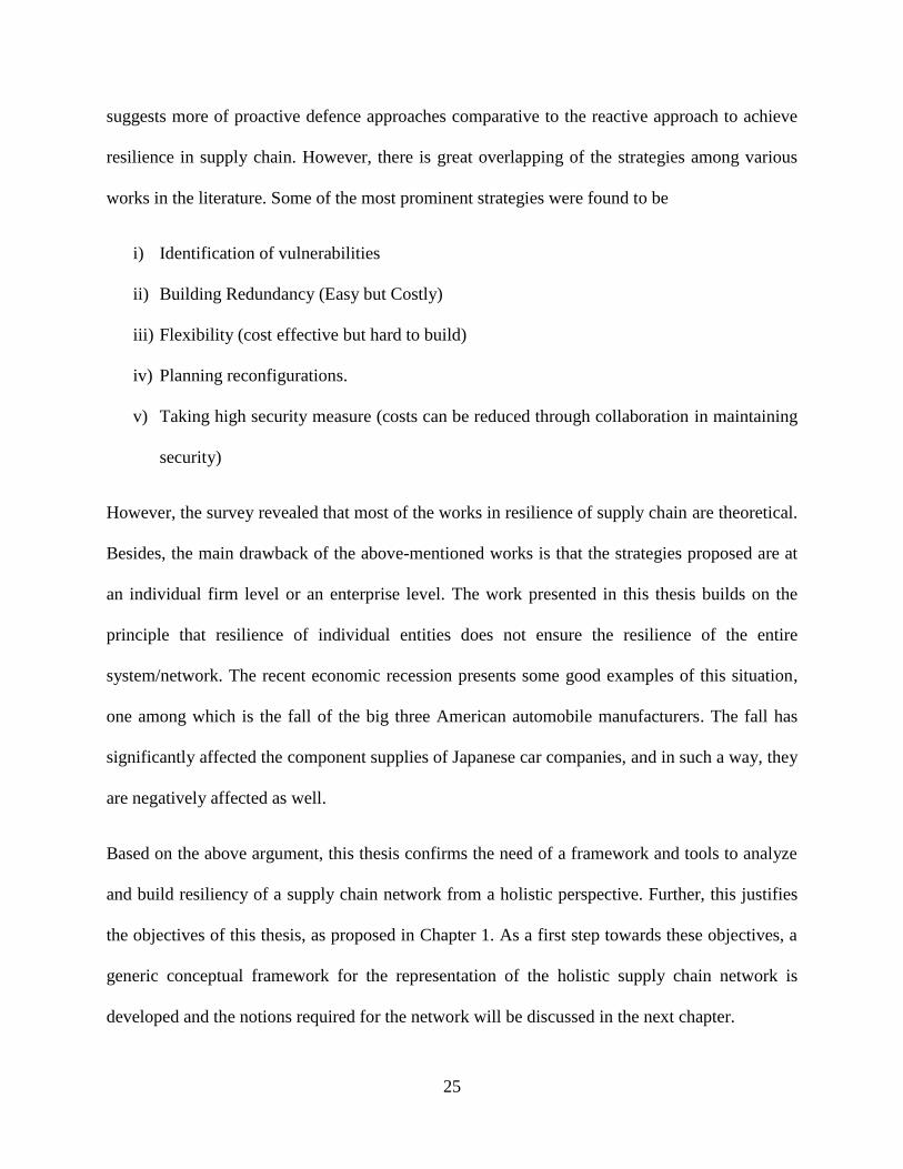
Figure 3.1 Hierarchies of the Supply Chain Networks. ................................................................ 27
Figure 3.2: Components for survival of a firm. ............................................................................ 30
Figure 3.3: Graphical illustration of break-even point.................................................................. 31
Figure 3.4 Health states of a firm for members of a Supply Chain Network. .............................. 33
Figure 3.5: Sample of the proposed Supply Chain Network Representation. .............................. 34
Figure 3.6 Sample disruption sequence in a supply chain network. ............................................. 37
Figure 3.7: Recovery module for sharing of redundant resources. ............................................... 40
Figure 4.1: Elements of a Petri net................................................................................................ 45
Figure 4.2: Demonstration of enabled transitions. ........................................................................ 46

xi
Figure 4.3: Differentiating tokens using Coloured Petri Nets ...................................................... 49
Figure 4.4 Use of Timed Petri net to model periodic events. ....................................................... 50
Figure 4.5: (Alternative 1) Hierarchical Petri nets for representing a supply chain network. ...... 53
Figure 4.6: (Alternative 2) Hierarchical Petri nets for representing a supply chain network. ...... 54
Figure 4.7: General flow of processes of an individual firm in a supply chain. ........................... 56
Figure 4.8: Basic features and notions of CPN tools. ................................................................... 57
Figure 4.9: Petri net for the member in a supply chain network. .................................................. 60
Figure 5.1 Conceptual representation of an automobile supply chain network example. ............ 67
Figure 5.2: Petri net model of a sample run of an automotive industry example. ........................ 74

1
Chapter 1 Introduction
1.1 Motivation
Over the past few decades, manufacturing strategies have evolved continuously to satisfy the
four major attributes of the consumer products namely their (1) Cost, (2) Quality, (3) Usability
and (4) Availability (or delivery time). The supply chain management has played a vital role in
delivering the complimentary support to achieve the aforementioned attributes. During the
1980‟s and 1990‟s, supply chain management was merely treated as a problem of intra-
organizational logistical management. Most of the models were solved for the optimal lot size
(Adler and Nanda, 1974; Afentakis and Gavish, 1986; Zipkin, 1991; Shinn, 1997), order quantity
(Emmett and Lodree, 2007) and architectural decisions to reduce the total channel costs.
However, the 9/11 terror attacks, the recent financial crisis and other major crisis have proved
that there is interaction and interdependency of the supply chains and a need to focus on building
resiliency (in general, the ability of the system to recover from damage or disruption) of the
system. On the other hand, factors such as core competency, globalization, improved
transportation structure & services, and ever growing information and communication
technologies have gradually reframed the supply chains to form strong interacting inter
organizational supply chain networks (Lu and Wang, 2008). Amidst these conditions, most
organizations are still focused on the vertical integration of various levels of their own supply
chain and there was very little consciousness on the interception of different supply chains.
Although literature has discussed some ways of improving resiliency of an individual firm it

2
lacked to capture a holistic view of the supply chain network. Pertaining to this condition, this
work proposes to improve resiliency of a supply chain network from a system‟s perspective
rather concentrating on an individual firm. In order to pursue this goal, the following research
objectives have been laid out in the next section of this chapter.
1.2 Objectives
1: Establish an effective definition for the supply chain network and explore the scope of
resiliency in the supply chain network.
2: Develop a framework to have a generic representation that could capture both structural and
behavioural elements of a supply chain network.
3: Identify the possible loopholes that compromise resiliency of a supply chain network and their
possible solution strategies.
4: Test the feasibility and adapt the aforementioned framework into an operational tool to
provide the scope for simulation and prediction of real life scenarios in supply chain network.
1.3 Research Methodology
A research methodology called the systematic review technique is used for the comprehensive
coverage and analysis of the related literature. According to (Biolchini et al., 2007), the term
„systematic review‟ is used to refer to a specific methodology of research, developed in order to
gather and evaluate the available evidence pertaining to a focused topic. It represents a secondary
study that depends on primary study results to be accomplished. In particular, this methodology
will be applied to identify the definition of resiliency with respect to supply chain network and to
classify the existing strategies of resiliency in the field of supply chain management. The

3
remaining work will be based on the simulation and demonstration of the conceptual framework
built to represent the supply chain network. For this purpose, Petri nets, a discrete event based
graphical simulation and formulization tool, is selected as one of the most suitable forms to
capture the dynamic behaviour of a supply chain network. To add further validity to the model
developed, case-based tests are performed to demonstrate the feasibility and possible benefits of
the model proposed in this work.
1.4 Organization of the Thesis
The remainder of this thesis is laid out into five chapters as follows:
Chapter 2: This chapter introduces the basic knowledge about supply chain management,
followed by a comprehensive understanding of the term resilience in a general sense. Then, it
proceeds to details through the literature review by applying the systematic review technique as
mentioned in the section 1.3. This chapter finally converges to the existing research issues in the
present supply chain network scenario with respect to resiliency, thus providing necessary
directions for further research work. It is to be noted that the literature review regarding the Petri
nets and its software are not included in this chapter. They will be discussed along with the
application of them in later chapters.
Chapter 3: This chapter builds upon the concepts and principles gathered from the literature
review of Chapter 2. A generic conceptual framework for the representation of the supply chain
network is developed and the notions required for the same are discussed. The framework
centers on the sharing of “economy health status” of each of the member firms with other
member firms in a supply chain network. Further, the need and utility of such a framework for
resiliency of the supply chain is argued by comparing the supply chain view from an individual

4
firm perspective (which is the contemporary view) with a network (holistic) perspective (which
is advocated in this thesis).
Chapter 4: In this chapter, the possible simulation tools for the realization of the framework
proposed in Chapter 3 are contemplated and choice of Petri nets is justified. Later, a brief
background of Petri nets and its extensions in literature are discussed. The mechanisms needed
for the application of the concepts of Petri nets to the proposed framework is illustrated. Further,
the Petri net models are realized through a software program (for modeling and simulating Petri
nets) called the CPN tools. An introductory section to explain the basic elements and functions of
the CPN tools software is also included in this chapter.
Chapter 5: This chapter validates the use of Petri net models proposed in Chapter 4 through
their application on two selected case studies.
Chapter 6: The final chapter discusses the contributions, limitations and future work.
Appendix A: This section contains the details of the Petri net simulation tool.

5
Chapter 2 Background and Literature Review
2.1 Introduction
This chapter introduces the basic knowledge about supply chain management in section 2.2,
followed by a comprehensive understanding of the term “resilience” in a general sense. A
comprehensive definition of the resilient system in the engineering context is also proposed at
the end of this section. Then, the chapter proceeds to two systematic reviews detailed in Section
2.3 and Section 2.4, respectively. The first review (Section 2.3) is regarding the analysis of the
term “Supply Chain Network” as referred to in the supply chain literature. The second covers the
works focused on resilient supply chains. This chapter finally converges to the existing research
issues in the present supply chain network scenario with respect to resiliency, thus providing
necessary directions for further research work, a part of which have been defined as the research
objectives of the thesis.
2.1.1 Supply Chain Management
In general, a supply chain is group of entities that are involved in a chain of processes concerning
the procurement of raw materials or components, their conversion or assembly into a product and
delivery of the final product to a customer. Lamming (2000) referred the origins of “supply chain
management (SCM)” to the early 1980‟s when it only represented the management of materials
across functional boundaries within an organization (Oliver and Webber, 1992; Houlihan, 1984)
but it was later extended to include “upstream” production chains and “downstream” distribution

6
channels (Womack et al., 1990; Womack and Jones, 1996; Harland and Clark, 1990;
Christopher, 1992). The typical definition of the term supply chain management by Bowersox
and Closs (1996) is as follows:
“The supply chain refers to all those activities associated with the transformation and
flow of goods and services, including their attendant information flows, from the sources of
materials to end users. Management refers to integration of all these activities, both internal and
external”.
The activities and components of a traditional supply chain are shown in Figure 2.1.
Figure 2.1: Typical supply chain (obtained from website of Weber State University; accessed:
June 2010 - http://organizations.weber.edu/sascm/supply_chain.bmp).

7
Several costs exists in a supply chain such as cost for raw materials, ordering cost, inventory
holding cost, transportation costs and production/assemble costs (including the operating costs).
Traditionally, supply chain management aims to reduce the sum of these costs by coordinating
various activities in the supply chain. At the same time, it also tries to achieve customer
satisfaction by improving the delivery time, product quality and availability. For this purpose
several strategies have evolved over the history to facilitate these objectives.
1) Mass customization: the capability of companies to offer individually tailored products
or services on a large scale i.e. combining customization with mass production (Zipkin,
2001).
2) Lean practices: Reduction of wastes that are anything without adding value to the
supply chain. Several further notions are related to this lean philosophy, such as just in
time (JIT), total quality management (TQM), total preventive maintenance (TPM), and
human resource management (HRM). (Shah and Ward, 2003). For example, inventory is
considered to be one of the non-value adding entities and the appropriate practice of “Just
in Time” is adopted. It is noted that “Just in Time” approach aims to reduce the inventory
or work in process to zero.
3) E-commerce and Virtual Organizations: Some of the modern supply chains enhanced
with the power of the Internet and other communication systems embark these new
strategies to satisfy the demand of their customers. For more details on E-commerce and
Virtual Organizations, the reader is referred to the works of Pego-Guerra (2005), Meyer
and Taylor (2000) and Walker (2005).
Supply chain management is a vast topic and involves many other concepts. The above concepts
give only the basic ideas that are required for understanding this thesis work.

8
2.1.2 Resilience
In this section, definitions of resilience as defined in various fields of study are presented.
Thereafter, some key characteristics of resilience from these definitions are selected, which will
be later used for the systematic review of resiliency in supply chain literature.
(i) Resiliency in Material Science:
Resilience in material science is usually referred to the ability of the material to return to its
original shape after temporary deflection. The degree of recovery is measured on the speed of
recovery (Nagdi, 1993). The degree of resilience is also measured on the ratio of the energy
returned to energy applied to produce the deformation. Higher the ratio, higher is the resilience
of the material (Nagdi, 1993). This ratio can be viewed as proportional to the percentage of
rebound.
(ii) Human resilience:
A critical review by Luthar et al. (2000) referred resilience as to a dynamic process
encompassing positive adaptation within the context of significant adversity. They considered
the individuals exposure to significant threat or adversity and positive adaptation despite
disruption to the development process.
An interesting distinction between recovery and resilience patterns was made based on the
impact of a traumatic event on the normal functioning of the human as shown in Figure 2.2.
Figure 2.2 shows that a resilient individual does have major disruptions in normal function
during a traumatic event but the effect is mild. Medium level disruptions are absorbed for the
recovery pattern which tends to increase first and then reach normal levels ultimately. The other
two plots, delayed and chronic are considered to be patterns of non-resilient individuals.

9
Figure 2.2: Possible human responses after a traumatic event. (Adopted from Bonanno and
Mancini (2008)).
(iii) Ecological and Engineering Resilience:
Holling (1996) defines and distinguishes engineering resilience and ecosystem resilience as two
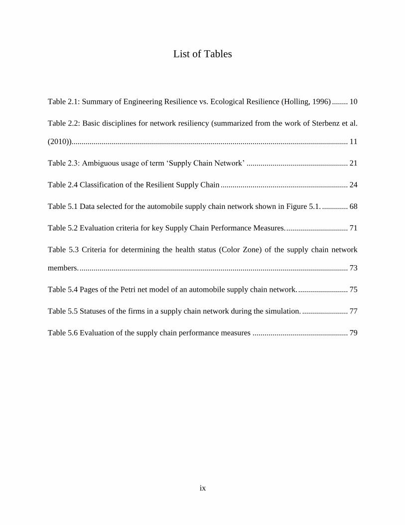
different and alternating paradigms. His ideas on these systems are shown in Table 2.1.
10
Table 2.1: Summary of Engineering Resilience vs. Ecological Resilience (Holling, 1996)
Engineering Resilience Ecological Resilience
Definition (focus on) Maintaining the function. Existence of the function
Attributes (Desired for fail-
proof design)
Efficiency,
Constancy and
Predictability
Persistence,
Change,
and Unpredictability
Stability Global optimum or one
equilibrium Steady State
exists
More than one equilibrium
states and systems flips states
in case of instabilities.
Measure of Resilience Resistance to Disturbance, and
Speed of Return to
equilibrium
The magnitude of disturbance
the system can absorb before
the system changes its
structure and attain a
controlled behavior.
In addition to the above work, Gao (2010) proposes a definition for engineering resilience based
on the concepts of system function and damage and further distinguishes it from the concepts
similar to resilience such as reliability, robustness, repairing, etc.
(iv) Information and communication Resilience:
Laprie (2008) identifies resilience in complex information and computer systems to have the
similar notion of ecological resilience as described by Holling (1973). For such system he
11
provides the following definition of resilience as “The persistence of the avoidance of failures
that are unacceptably frequent or severe, when facing changes.”
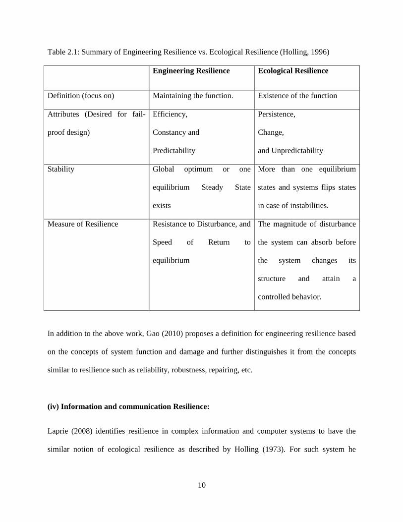
Sterbenz et al. (2010) describes the following two disciplines that serve as basis of network
resilience:
a) Challenge tolerance disciplines that deal with the design and engineering of systems that
continue to provide service in the face of challenges.
b) Trustworthiness disciplines that describe measurable properties of resilient systems.
The divisions of these disciplines are tabulated in table 2.2.
Table 2.2: Basic disciplines for network resiliency (summarized from the work of Sterbenz et al.
(2010))
Challenge tolerance Fault Tolerance (compensated through Redundancy)
Survivability (requires diversity)
Disruption tolerance
Traffic tolerance (accommodate sudden load)
Trustworthiness Dependability (availability and reliability)
Security (reduce unauthorized access)
Perform-ability
(v) Business resilience:
Hamel and Valikangas (2003) referred business resilience as a superior capacity to reinvent a
business model before circumstances forces to change. They further proposed the following
strategies for business resilience:

12
1. Anticipation of unexpected failures through close attention to the business environment.
2. Investment in diversity (products or services).
3. Constant exploration of new opportunities.
4. Maintaining the balance between optimization (a pursuit for efficiency) and exploration
of new opportunities.
(vi) Generic definition of the resilient system:
The definitions of resilience gathered from various fields are utilized to prescribe the
characteristics of a resilient system and build a comprehensive definition for the same. The
definition is also translated to a supply chain perspective.
a) Objective: The objective of resilient system should be to survive and maintain function
(at least partially) in the course of disruption. In the case of supply chain, survival can be
viewed as an equivalent to making profit, while the function of a supply chain is
described as to meet the demand with enough supply. Here, survival and function are
separated to capture a case where the supply chain meets the demand but the demand is
not sufficient to make enough profit for its survival.
b) Anticipation: A resilient system should have continuous anticipation for all kinds of
disruptions by paying close attention to the constant changes in its environment and at the
same time utilize the knowledge learned from the past disruptive events.
c) Estimation: Have the strong intent to estimate and prioritize the damages that could occur
from the anticipated disruptions.
d) Preparation: A resilient system should adopt a suitable resilient strategy or combination
of strategies as a preparation for defence from the possible disruptions. Some of the

13
resilient strategies as identified from the above study of resilience in various fields are
building diversity, flexibility, redundancy, security and safety measures, collaboration
and sharing of resources etc. The strategy selection is system, context and situation
dependent. As an extension of the distinction made by Holling (1996) between
engineering resilience versus ecological resilience, this article believes that the supply
chain systems occupy the intersection of these two paradigms (see Table 2.1) as it not
only deals with the social component in the form of interactions with suppliers and
customers but also concerns with the engineering values during the production and
manufacturing phase.
Combining the above characteristics, a generic definition of resilient system (also applicable to
supply chain systems) is derived as follows:
A resilient system is a system with an objective to survive and maintain function even
during the course of a disruption, provided with a capability to predict and assess the damage of
the possible disruptions, enhanced by strong awareness of its ever changing environment and
knowledge of the past events and thereby utilizing resilient strategies for defence against the
disruptions.
The proposed definition can be seen as a combination of the definitions of Zhang and Lin (2010)
and Hollnagel et al. (2006).
2.2 Supply Chain Network
In this section, the origin of the term “Supply Chain Network” is investigated and its usage in
literature is studied. Further, we contemplate the ambiguity in the usage of the term “Supply
Chain Network” existing in the literature. This is because the elements of a supply chain are

14
significantly clear; however it is not very vivid how the elements of the supply chain are
connected to form a supply chain network. To find answers to the above mentioned issues,
systematic review technique is adopted. The steps of the systematic review performed are
detailed from subsequent Subsections 2.2.1 to 2.2.5.
2.2.1 Selection of research article data bases
The following two online citation databases have been selected for the study.
1. Science Direct: www.sciencedirect.com.
2. SCOPUS: www.scopus.com
These two data sources comprehensively cover all the major journals and magazines in the fields
of supply chain, manufacturing, production, industrial engineering and operations research
including journals (e.g., European Journal of Operational Research, International Journal of
Production Research, Omega, IEEE, Management Science etc).
2.2.2 Keywords and Search Strategy
The three keywords supply, chain and network are used with the following combinations:
„supply network‟, „supply chain‟ and „network‟. The search is directed to all contents including
the title of the article, abstract and the keywords in all the relevant journals and magazines. There
was no restriction imposed on years of publication. This is done to find out the first use of term
“supply chain network”.
The search yielded a huge number of articles and after applying filters in the respective websites
Science direct data source search yielded 1027 articles and the distribution of the articles over
the years is shown in the following figure. Figure 2.3 shows the number of articles using the term

15
“supply chain network” on the vertical axis and the corresponding year of publication on the
horizontal axis.
Figure 2.3: Distribution of articles (in ScienceDirect database) using the term “Supply chain
Network”.
A similar search on the database of SCOPUS showed that 694 articles have used the term
„Supply Chain Network‟ and distribution of these articles is shown in Figure 2.4.
0
50
100
150
200
250
1986 1988 1990 1992 1994 1996 1998 2000 2002 2004 2006 2008 2010
Science Direct Search Results for "Supply Chain Network"
Number of citations
Year

16
Figure 2.4: Distribution of articles (in SCOPUS database) using the term “Supply chain
Network”.
The analysis of these graphs is presented in section 2.2.4 later.
2.2.3 Selection criteria and data collection
Since the number of articles found is enormous, only 48 articles were chosen for the analysis
based on their relevance to supply chain network and popularity (number of citations received).
The articles selection was also uniformly distribution over the years of publications proportional
to the number of articles for the respective years.
2.2.4 Analysis
A preliminary analysis was performed on the search results with the help of the plots shown in
Figure 2.3 and Figure 2.4, respectively. These plots indicate that the use of term „supply chain
0
20
40
60
80
100
120
140
160
1986 1988 1990 1992 1994 1996 1998 2000 2002 2004 2006 2008 2010
Scopus Search Results for "Supply Chain Network"
Number of citations
Year

17
network‟ became widely popular in the supply chain literature at the beginning of the years of
1998-1999. Moreover, its usage kept increasing over the years as seen in Figure 2.3 and Figure
2.4, respectively. It is to be noted that the drop in the curves in the last section of the plots is
because articles published only till the middle of the year 2010 were considered.
A further analysis was performed through the careful study of the selected 48 articles (listed in
Table 2.3). As for the origin of the term „supply chain network‟ the first among the authors to use
this term based on the search above were Billington and Davis (1992), Padillo and Brown
(1995), Huchzermeier and Cohen (1996). Correa and Miranda (1998), Chandra (1997), Lin et.al.
(1998), Ross et al. (1998), Fu-Renlin and Shaw (1998) Srinvasan and Moon (1999). However,
the first comprehensive definition and analysis of supply chain network was not recorded until
Fu-Renlin and Shaw (1998). According to them, “A supply chain network (SCN) is a network of
autonomous or semi-autonomous business entities involved, through upstream and downstream
links, in the different processes and activities that produce goods or services to customers.”
Further, they classified supply chain network into three types based on seven attributes.
However, such classification has not included the structural information of the network which
differentiates different supply chain systems. This is especially important because the increasing
usage of the term „supply chain network‟ combined with no clear definition or classification on
its structure might cause some trouble for future researchers to identify relevant literatures. To
address this concern, this thesis identified three possible network structures that might have been
referred as to supply chain networks by the earlier researchers in this field. These three structures
are illustrated as follows:
The first kind of structure contains a tree like structures. In this structure various branches evolve
from a single node reaching various parts of the network. This structure is usually seen when the
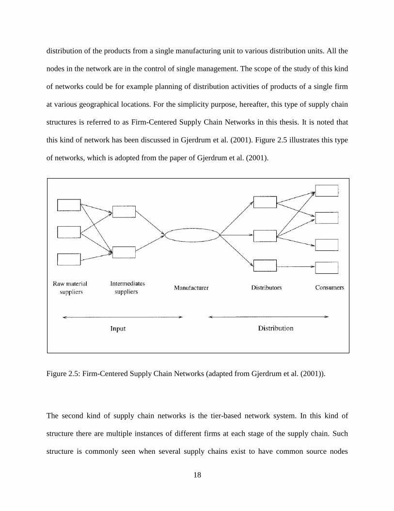
18
distribution of the products from a single manufacturing unit to various distribution units. All the
nodes in the network are in the control of single management. The scope of the study of this kind
of networks could be for example planning of distribution activities of products of a single firm
at various geographical locations. For the simplicity purpose, hereafter, this type of supply chain
structures is referred to as Firm-Centered Supply Chain Networks in this thesis. It is noted that
this kind of network has been discussed in Gjerdrum et al. (2001). Figure 2.5 illustrates this type
of networks, which is adopted from the paper of Gjerdrum et al. (2001).
Figure 2.5: Firm-Centered Supply Chain Networks (adapted from Gjerdrum et al. (2001)).
The second kind of supply chain networks is the tier-based network system. In this kind of
structure there are multiple instances of different firms at each stage of the supply chain. Such
structure is commonly seen when several supply chains exist to have common source nodes

19
(suppliers) and destination (customers) nodes. The nodes in this kind of network are usually
independent and not all under the control of a single enterprise. The scope of the study of such
networks is usually towards the competition among the members of the same tier level and
partner selection strategies. This kind of structure was referred to in the work of Tsiakis et al.
(2001), as shown in Figure 2.6.
Figure 2.6: Industry Centered Supply Chain Networks (adapted from Tsiakis et al. (2001)).
This kind of networks is centered on a particular industrial sector of products (for example
automotive sector). The networks of this kind do not extend their reach beyond their industrial
sector.
The last type of structure of supply chain networks this thesis is interested to study is referred to
as Inter-industrial Supply Chain Network Structure. Their structure considers a broader range of
supply chain networks where the network is not confined just to a single industrial sector; rather
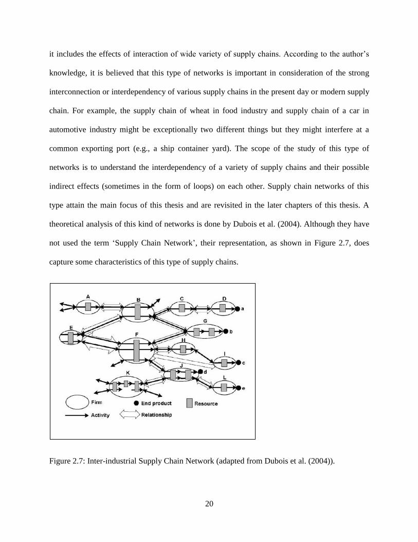
20
it includes the effects of interaction of wide variety of supply chains. According to the author‟s
knowledge, it is believed that this type of networks is important in consideration of the strong
interconnection or interdependency of various supply chains in the present day or modern supply
chain. For example, the supply chain of wheat in food industry and supply chain of a car in
automotive industry might be exceptionally two different things but they might interfere at a
common exporting port (e.g., a ship container yard). The scope of the study of this type of
networks is to understand the interdependency of a variety of supply chains and their possible
indirect effects (sometimes in the form of loops) on each other. Supply chain networks of this
type attain the main focus of this thesis and are revisited in the later chapters of this thesis. A
theoretical analysis of this kind of networks is done by Dubois et al. (2004). Although they have
not used the term „Supply Chain Network‟, their representation, as shown in Figure 2.7, does
capture some characteristics of this type of supply chains.
Figure 2.7: Inter-industrial Supply Chain Network (adapted from Dubois et al. (2004)).

21
The three categories of supply chain networks discussed above are used to classify the 47
selected literatures and are tabulated in Table 2.3.
Table 2.3: Ambiguous usage of term „Supply Chain Network‟
Firm-Centered Supply Chain Networks
Huchzermeier and Cohen (1996), Zhou et al. (1998), Ross et al. (1998), Dogan and Goetschalckx
(1999), Min and Melachrinoudis (1999), Mirhassani et al. (2000), Gjerdrum et.al (2001), Dong
and Chen (2001), Raghavan and Viswanadham (2001), Zhou et al. (2002), Dong et al.(2004),
Eskigun et al. (2005), Melo et al. (2006), Choi et al. (2006), Liu and Zhou (2007), Dong and
Peng (2007), Chiou (2007), Romeijn et al. (2007), Melo et al. (2009),Che et al. (2009).
Industry Centered Supply Chain Networks
Min and Melachrinoudis (1999), Rupp and Ristic (2000), Tsiakis et al. (2001), Nagurney et al.
(2002), Cakravastia et al. (2002), Lancioni et al. (2003), Chen et al. (2003), Wathne and Heide
(2004), Chen (2004), Dong et al. (2004), Chan and Chan (2004), Jain et.al (2004), Santoso et al.
(2005), Altiparmak et al. (2006), Jiao et al. (2006), Patnayakuni et al. (2006), Sha and Che
(2006), Ding et al. (2006).
Inter-industrial Supply Chain Networks
Lin and Shaw (1998), Lin et al. (1999), Mirhassani et al. (2000), Cox (2004), Fandel and
Stammen (2004), Ranganathan et al. (2004), Beamon and Fernandes (2004), Surana et al.
(2005), Sanders (2005), Wuming et al. (2009).
Table 2.3 includes those that use the term „supply chain network‟ in the literature but use it in an
ambiguous manner.
22
2.2.5 Summary and Discussion of the Review
In summary, the term „supply chain network‟ has been widely used in the literature. Its usage is
ever-growing and so is its ambiguity. Although some classifications of supply chain networks are
available in the literature (Lin and Shaw, 1998; Wuming et al., 2009), no clear terminology is
available to distinguish the supply chain network structures and their respective scope of
purpose. This review suggests three types of supply chain networks based on their structure and
scope of purposes; further these are identified with strong informative terminology namely, Firm
Centered Supply Chain Networks, Industry Centered Supply Chain Networks and Inter-industrial
Supply Chain Network. Some of the prominent works in the field of Supply chain Network are
also grouped into the three categories of Supply Chain Networks proposed in Section 2.2.4. It is
believed that this classification provides a platform for future researchers to identify and present
their works in most relevant sections of the supply chain literature.
2.3 Supply Chain and Resilience
In this section a review of the works relating to the application of resilience in the field of supply
chain management is presented. A similar systematic review used in Section 2.2 was adopted for
this review. The databases and search methodology remained the same. While the keywords used
are shifted to the various combinations of the words Supply chain, Supply chain network,
Resilience, Resilient, Resiliency. For the selection criteria, only the works that address resilience
and its related issues in supply chains are selected. Besides relevance, the number of citations
was also taken into account. As a result, forty three articles are selected for the analysis and the
classification is done into four categories. These categories are developed based on the
characteristics proposed in the definition of resilient system in Section 2.2. The categories are as
follows:
23
1) Awareness and anticipation: Articles that stress on the identification and awareness
practices of existing vulnerabilities and upcoming disasters in a supply chain are placed
in this category.
2) Estimation and decision: The articles that are focused on computation regarding the
effect of a disruption or effect of adopting alternative mitigation strategies.
3) Proactive Defence: Proactive strategies are ones that are in action even before a
disruption takes places.
4) Reactive Defence: Reactive strategies are ones that are designed to perform defensive
action after a damage or disruption to the system.
Using the above four categories, forty three articles relating to the literature of resilient supply
chain are selected and grouped as shown in Table 2.4. If an article is placed in more than one
group, it has impact on all the categories in which it is placed.
24
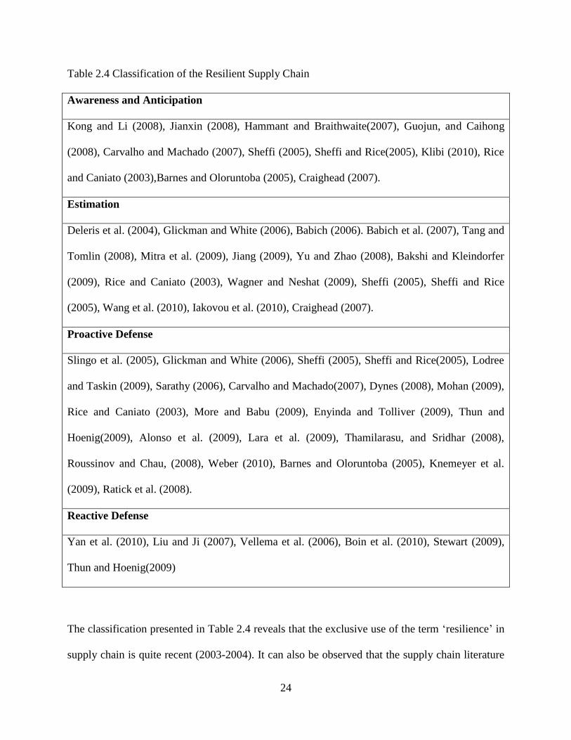
Table 2.4 Classification of the Resilient Supply Chain
Awareness and Anticipation
Kong and Li (2008), Jianxin (2008), Hammant and Braithwaite(2007), Guojun, and Caihong
(2008), Carvalho and Machado (2007), Sheffi (2005), Sheffi and Rice(2005), Klibi (2010), Rice
and Caniato (2003),Barnes and Oloruntoba (2005), Craighead (2007).
Estimation
Deleris et al. (2004), Glickman and White (2006), Babich (2006). Babich et al. (2007), Tang and
Tomlin (2008), Mitra et al. (2009), Jiang (2009), Yu and Zhao (2008), Bakshi and Kleindorfer
(2009), Rice and Caniato (2003), Wagner and Neshat (2009), Sheffi (2005), Sheffi and Rice
(2005), Wang et al. (2010), Iakovou et al. (2010), Craighead (2007).
Proactive Defense
Slingo et al. (2005), Glickman and White (2006), Sheffi (2005), Sheffi and Rice(2005), Lodree
and Taskin (2009), Sarathy (2006), Carvalho and Machado(2007), Dynes (2008), Mohan (2009),
Rice and Caniato (2003), More and Babu (2009), Enyinda and Tolliver (2009), Thun and
Hoenig(2009), Alonso et al. (2009), Lara et al. (2009), Thamilarasu, and Sridhar (2008),
Roussinov and Chau, (2008), Weber (2010), Barnes and Oloruntoba (2005), Knemeyer et al.
(2009), Ratick et al. (2008).
Reactive Defense
Yan et al. (2010), Liu and Ji (2007), Vellema et al. (2006), Boin et al. (2010), Stewart (2009),
Thun and Hoenig(2009)
The classification presented in Table 2.4 reveals that the exclusive use of the term „resilience‟ in
supply chain is quite recent (2003-2004). It can also be observed that the supply chain literature
25
suggests more of proactive defence approaches comparative to the reactive approach to achieve
resilience in supply chain. However, there is great overlapping of the strategies among various
works in the literature. Some of the most prominent strategies were found to be
i) Identification of vulnerabilities
ii) Building Redundancy (Easy but Costly)
iii) Flexibility (cost effective but hard to build)
iv) Planning reconfigurations.
v) Taking high security measure (costs can be reduced through collaboration in maintaining
security)
However, the survey revealed that most of the works in resilience of supply chain are theoretical.
Besides, the main drawback of the above-mentioned works is that the strategies proposed are at
an individual firm level or an enterprise level. The work presented in this thesis builds on the
principle that resilience of individual entities does not ensure the resilience of the entire
system/network. The recent economic recession presents some good examples of this situation,
one among which is the fall of the big three American automobile manufacturers. The fall has
significantly affected the component supplies of Japanese car companies, and in such a way, they
are negatively affected as well.
Based on the above argument, this thesis confirms the need of a framework and tools to analyze
and build resiliency of a supply chain network from a holistic perspective. Further, this justifies
the objectives of this thesis, as proposed in Chapter 1. As a first step towards these objectives, a
generic conceptual framework for the representation of the holistic supply chain network is
developed and the notions required for the network will be discussed in the next chapter.

26
Chapter 3 Conceptual Framework for Supply Chain Networks
3.1 Introduction
This chapter focuses on definition of a conceptual framework with its emphasis on a holistic
view of resilience in a supply chain network. The key argument for the need of such a framework
has already been discussed in chapter 2 and in particular is the principle that the resilience of
individual entities does not ensure the resilience of an entire system/network. In this thesis,
communication (information sharing) among members of a supply chain network is taken as a
fundamental concept to promote resiliency in a supply chain network, which is also seen a
significant departure of this thesis from many others in literature. Specifically, this thesis focuses
on the extraction of information regarding the origin of disruptions and possible propagation of
their effects in an entire supply chain network to a certain depth and breadth. The first step
towards such a framework is to have a generic representation of a supply chain network which
can capture interactions at a level of Inter-industrial Supply Chain Networks (see chapter 2). The
choice of this level of description is apparent in the context of a holistic vision as it positions at a
higher hierarchical level than the other two types of supply chain networks (i.e., Firm level
Supply Chain Networks and Industry centered Supply Chain Networks discussed in chapter 2).
Figure 3.1 illustrates that the firm level and industry centered supply chain networks are merely
subsets of the Inter-Industrial supply chain networks.
27
Figure 3.1 Hierarchies of the Supply Chain Networks.
However, the integration of a wide variety (in terms of type of products, services and resources
involved) of supply chains into a single framework demands a common attribute (language) to
facilitate the detection and communication of effects among supply chains. For this purpose, this
thesis work proposes “economic health” of a member in the supply chain network as a common
means to detect and measure disruptions, further it is an aggregative attribute of all possible
disruptions such as damage to transportation infrastructure (transportation delays), excess
inventory, availability of human or machine resources (manufacturing delays), low demand for
products, and so on. For simplicity, hereafter, this thesis uses the term “health” to refer to
“economic health”.
In what follows, Section 3.2 describes the proposed conceptual framework and several relevant
notions, including the health of a supply chain network. In Section 3.3, hypothetical examples
28
are employed to illustrate possible applications of the proposed framework to improve resiliency
in a supply chain network.
3.2 Conceptual Model
In this section, a conceptual framework is proposed to capture the structure and the behaviour of
a supply chain network. At first, the components and flows in a supply chain are identified. A
supply chain usually starts with procurement of raw materials through a manufacturing phase
and distribution of the materials and it ends with consumption and disposal of a product or
service. Various firms (e.g., mining firms, manufacturing firms, transportation service providers,
retailers, etc.) are involved to carry out these supply chain functions, and these firms are
components of a supply chain. Members of the supply chain can have two types of relationships
with other members of the supply chain. One relationship is that a firm is a supplier to other
members in the supply chain, and the other relationship is that a firm is a customer to other firms.
Here, the supplier firm is used in a general sense, meaning that the thing to be supplied could be
material, human or machine resource, knowledge, a service or combinations of any of them (Liu
et al., 2006). An existing relationship between any two firms in a supply chain network may have
any of the following flows:
1) Physical flows: Flows from the supplier to the consumer firm.
2) Monetary flow: From the consumer firm to the supplier firm.
3) Information flow: Information flow in the form of communications in both directions.
The three flows are supported by various infrastructures. In this thesis, infrastructure is a
common front or a supporting interface that is utilized by various firms to enable the
aforementioned flows in the network. For example, an infrastructure for the material flow is the

29
transportation system (e.g., roads, rails, seaports, airports, etc) (Wang et al., 2010a; Wang et al.,
2010b). A satellite or the internet, telephone lines could be infrastructures for the information
flows. Financial institutions such as banks could be kinds of infrastructures that facilitate the
money flow in a supply chain network. The infrastructure in a supply chain network cannot be
ignored, because many supply chains share the infrastructure for its services and its failure could
mean a simultaneous disruption to many supply chains. In the proposed framework, the
organization for managing the infrastructure will be regarded as a member in the entire network.
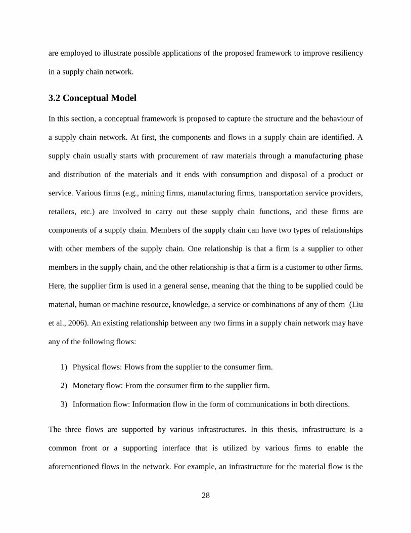
It is proposed that Darwin‟s theory of survival (Darwin, 1872; Headley, 1909) accounts for the
behaviour of each member in a supply chain network. In particular, survival of a firm is linked
with its profit gained while it performs its specific supply chain function. Further, the profit is
strongly coupled with the primary factors (i.e., supply and demand), generated by its
neighbouring suppliers and customers, respectively. In addition to these two factors, availability
and efficiency of its internal resources required for conversion of inputs to outputs are also
related to the profit. Consequently, failure of a firm in a supply chain network is caused by
damage to any of these three (i.e., supply, demand and internal resource) aspects; see also the
illustration in figure 3.2. Gunasekaran (2001) has related these three aspects to improving
competitiveness and the prospects of survival in an increasing volatile and global business
environment, but in his idea, the three are not explicitly related to the profit.
30
Figure 3.2: Components for survival of a firm.
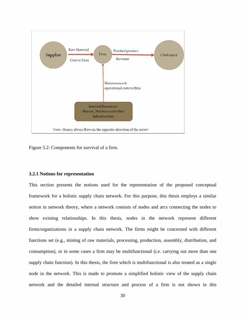
3.2.1 Notions for representation
This section presents the notions used for the representation of the proposed conceptual
framework for a holistic supply chain network. For this purpose, this thesis employs a similar
notion in network theory, where a network consists of nodes and arcs connecting the nodes to
show existing relationships. In this thesis, nodes in the network represent different
firms/organizations in a supply chain network. The firms might be concerned with different
functions set (e.g., mining of raw materials, processing, production, assembly, distribution, and
consumption), or in some cases a firm may be multifunctional (i.e. carrying out more than one
supply chain function). In this thesis, the firm which is multifunctional is also treated as a single
node in the network. This is made to promote a simplified holistic view of the supply chain
network and the detailed internal structure and process of a firm is not shown in this
31
representation; in other words, a firm in a supply chain network or a node in a network is treated
as a black box. However, the health of each firm or node is explicitly represented, and in fact the
health information will be supposed to be shared by all the member firms in the network. It is to
be noted that the proposed representation takes a graphical form where a node represents a firm,
and different states of the health of the firm is represented by different colors.
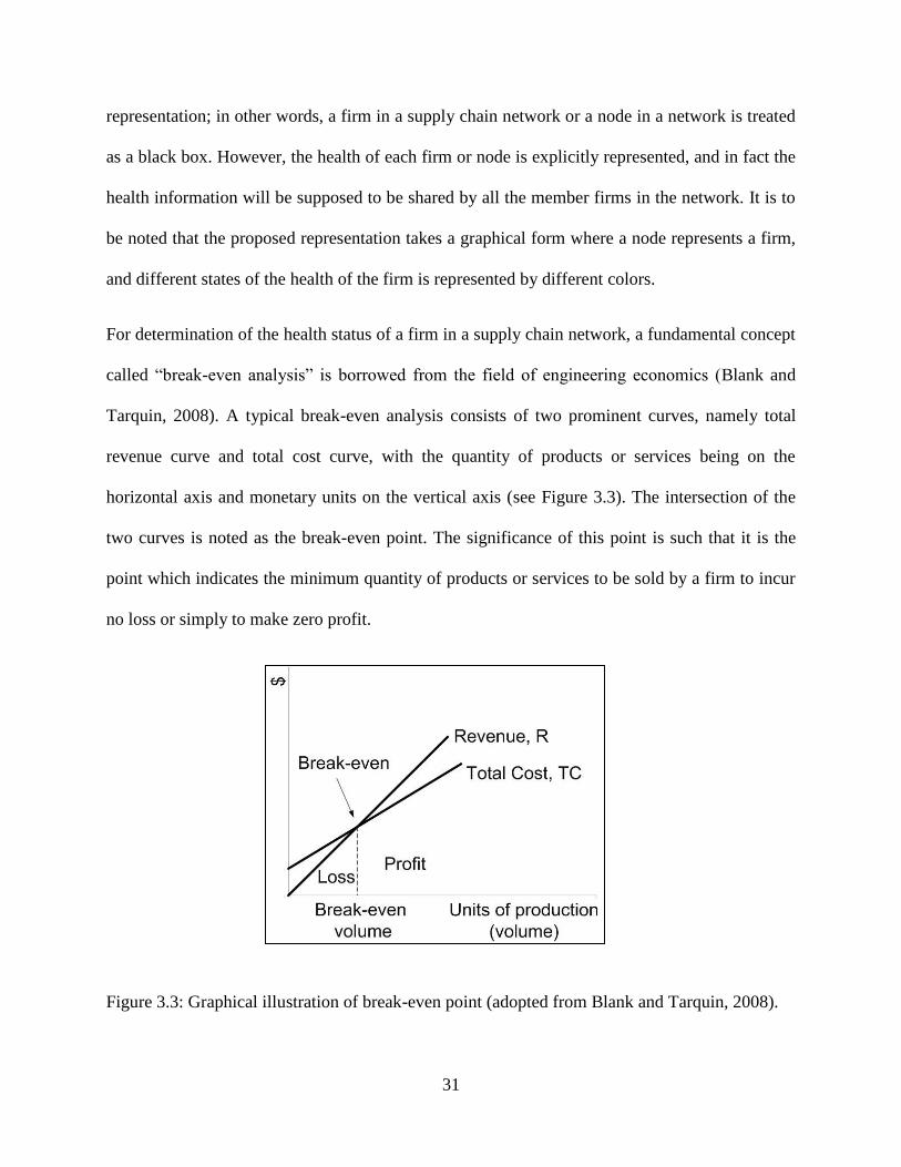
For determination of the health status of a firm in a supply chain network, a fundamental concept
called “break-even analysis” is borrowed from the field of engineering economics (Blank and
Tarquin, 2008). A typical break-even analysis consists of two prominent curves, namely total
revenue curve and total cost curve, with the quantity of products or services being on the
horizontal axis and monetary units on the vertical axis (see Figure 3.3). The intersection of the
two curves is noted as the break-even point. The significance of this point is such that it is the
point which indicates the minimum quantity of products or services to be sold by a firm to incur
no loss or simply to make zero profit.
Figure 3.3: Graphical illustration of break-even point (adopted from Blank and Tarquin, 2008).
32
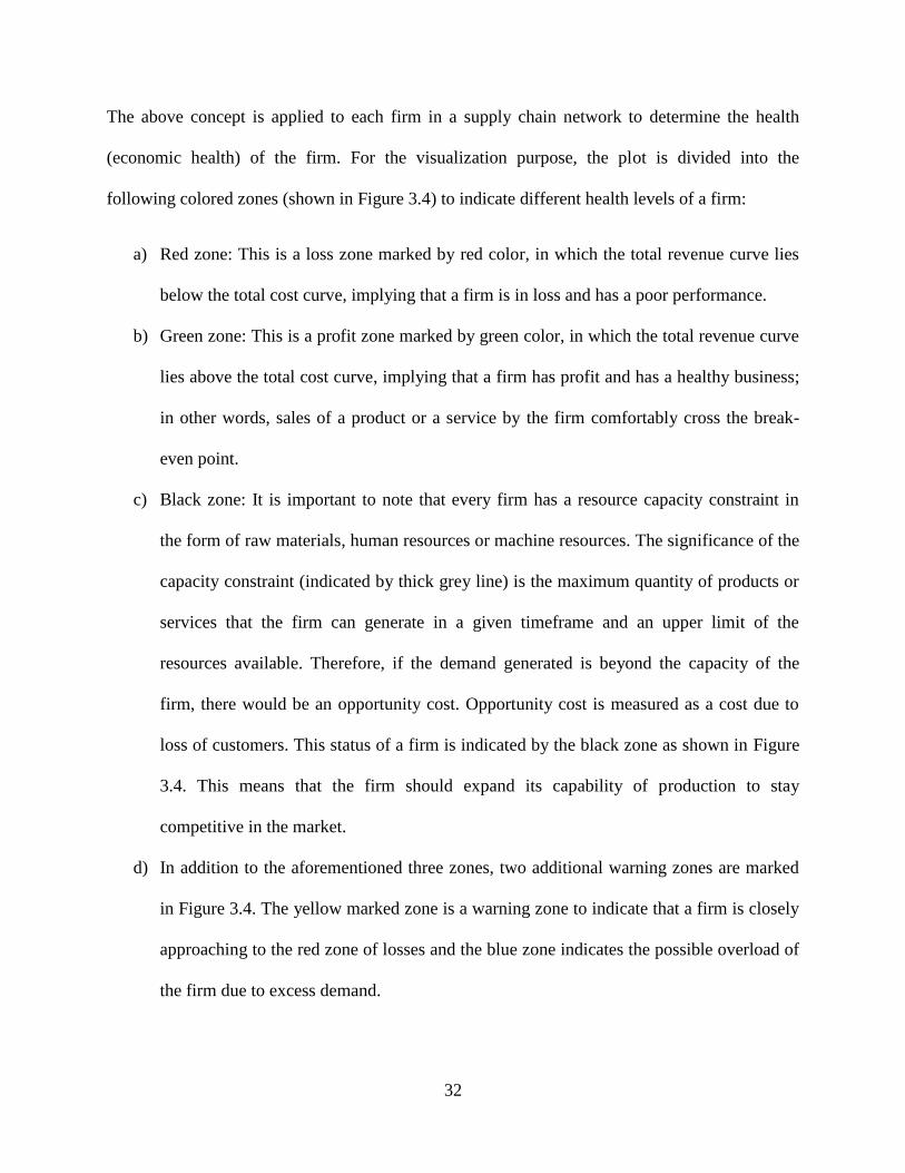
The above concept is applied to each firm in a supply chain network to determine the health
(economic health) of the firm. For the visualization purpose, the plot is divided into the
following colored zones (shown in Figure 3.4) to indicate different health levels of a firm:
a) Red zone: This is a loss zone marked by red color, in which the total revenue curve lies
below the total cost curve, implying that a firm is in loss and has a poor performance.
b) Green zone: This is a profit zone marked by green color, in which the total revenue curve
lies above the total cost curve, implying that a firm has profit and has a healthy business;
in other words, sales of a product or a service by the firm comfortably cross the break-
even point.
c) Black zone: It is important to note that every firm has a resource capacity constraint in
the form of raw materials, human resources or machine resources. The significance of the
capacity constraint (indicated by thick grey line) is the maximum quantity of products or
services that the firm can generate in a given timeframe and an upper limit of the
resources available. Therefore, if the demand generated is beyond the capacity of the
firm, there would be an opportunity cost. Opportunity cost is measured as a cost due to
loss of customers. This status of a firm is indicated by the black zone as shown in Figure
3.4. This means that the firm should expand its capability of production to stay
competitive in the market.
d) In addition to the aforementioned three zones, two additional warning zones are marked
in Figure 3.4. The yellow marked zone is a warning zone to indicate that a firm is closely
approaching to the red zone of losses and the blue zone indicates the possible overload of
the firm due to excess demand.

33
Figure 3.4 Health states of a firm for members of a Supply Chain Network.
Using the notions discussed above, a sample supply chain network is explained using Figure 3.5.
The firms are represented by circular nodes connected by arrows with the state of health
indicated by a color dot at the center of each node (initially all the firms are show to be in green
zone indicating a healthy supply chain network).

34
Figure 3.5: Sample of the proposed Supply Chain Network Representation.
Figure 3.5 shows various supply chain network members/firms (e.g., suppliers, production firms,
distribution centers, transportation firms, etc) responsible for the flow of four different products.
The four products are named after the raw materials (A, B, and C) used for their production. For
example, the product made with raw materials B and C is denoted by P (B, C). Also, it is to be
noted that products of one firm may become inputs for the product of another firms. For
example, the product P (A) from the Producer 2 is used as an input to produce the product P` (A)
(i.e. P`(A)=P(P(A)) by Producer 3. Other members in the supply chain network such as
transportation firm and distribution center just pass on products to the next stage without any
modification to the products. For such firms, inputs and outputs are the same. All the
members/nodes in a supply chain network are assumed to be independent in ownership and as

35
mentioned early, the arrow moving away from the node is a source of revenue and the arrow
coming towards a node are sources of costs to the firm. For example, considering Producer 1 in
Figure 3.5, the incoming arrows indicate the flow of materials A, B, C from the suppliers and are
a form of expenditures to the production firm (Producer 1). The arrows indicating the flow of
products P(B,C), P(A,B,C) and P(C) originating from the Producer 1 node are sources of its
revenue. Further, it may be stated that a disruption in the incoming arrows means a disruption in
the supply of materials to the firm (i.e., a probable opportunity cost) and disruption in the
outgoing arrows implies disruption at the demand side, hence loss of revenue.
3.3 Application
The above proposed framework can have the following applications:
3.3.1 Detection of disruption and its spread
The early awareness/information regarding the origin and propagation of effects of a disruption
contributes to better resiliency of the system. These characteristics give the system or component
of a system more time to respond; hence less could be the damage (or further damage) and easier
is the recovery of the system. This application is further illustrated through a comparison of the
awareness at the firm level (meaning awareness only after the disruption reaches the neighboring
nodes) to the global awareness of disruptions over an entire supply chain network. Consider the
following hypothetical disruption at the supplier 1 node in the supply chain network shown in
Figure 3.5. A series of network diagrams (see Figure 3.6 (a) to (f)) are used to show a possible
propagation of this disruption in the supply chain network starting at supplier 1 shown in Figure
3.5. In Figure 3.6(a), the health status of Supplier 1 is indicated by red (i.e. services/products
below the breakeven point). The failure of Supplier 1 affects the supply of material “A” to the
Producer 1 and Producer 2, respectively, and disables them to produce products P(A,B,C) and

36
P(A), respectively. These failures are updated in Figure 3.6 (b) where the statuses of Producer 2
and customer firm 3 are changed to red. However, Producer 1 is shown to have a healthy status
(green), given the diversity in its product line (i.e. it has the other products P (B, C) and P(C) to
generate revenue and do not require material “A”). Figures 3.6(c) and 3.6(d) show the failure of
the nodes (Producer 3 and transportation firm) following the disruption in the supply of material
A. The failure of Producer 3 follows the failure of Producer 2 since its only product P` (A) uses P
(A) as input. As for the transportation firm, its survival is dependent on transportation services
provided for both the products P` (A) and P (B, C). However, if a major portion of the revenue is
from the transportation service provided to product P` (A), then there exists the possibility of
failure of this node due to the failure of Producer 3. The failure of the transportation firm further
causes disruption to the distribution center activities and ultimately effect the Producer 1 (see
Figure 3.6 (e) and 3.6(f)).
Observing the disruption pattern of the supply chain network in Figure 3.6, the first impact on
Producer1 is felt as soon as the Supplier 1 node fails. However, the loss of only one of its
product P (A, B, C) does not affect its health status during this event (see Figure 3.6 (b)). Further
down the time scale, the disruption propagates through the supply chain of another product P`
(A) and effects the distribution center of the product P (B, C) and ultimately effects the health
status of the node Producer 1(see Figure 3.6 (b)). Therefore, the failure or the disruption of the
Supplier 1 has two effects on Producer 1. The first one is a direct effect and immediate in the
form of supply shortage of material “A”. The second effect takes some time to propagate through
the supply chain of product P` (A) before reaching the neighboring node (the distribution center)
of Producer 1. The early prediction of this indirect effect is possible if and only if Producer 1 has
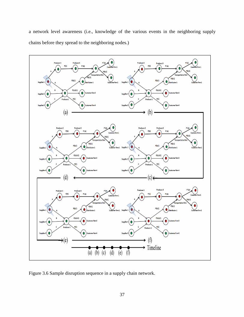
37
a network level awareness (i.e., knowledge of the various events in the neighboring supply
chains before they spread to the neighboring nodes.)
Figure 3.6 Sample disruption sequence in a supply chain network.
38
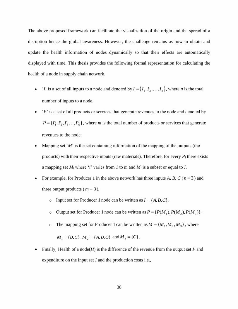
The above proposed framework can facilitate the visualization of the origin and the spread of a
disruption hence the global awareness. However, the challenge remains as how to obtain and
update the health information of nodes dynamically so that their effects are automatically
displayed with time. This thesis provides the following formal representation for calculating the
health of a node in supply chain network.
„I‟ is a set of all inputs to a node and denoted by nIIII ,,, 21 , where n is the total
number of inputs to a node.
„P‟ is a set of all products or services that generate revenues to the node and denoted by
},,,{ 321 mPPPPP , where m is the total number of products or services that generate
revenues to the node.
Mapping set „M‟ is the set containing information of the mapping of the outputs (the
products) with their respective inputs (raw materials). Therefore, for every Pi there exists
a mapping set Mi where „i‟ varies from 1 to m and Mi is a subset or equal to I.
For example, for Producer 1 in the above network has three inputs A, B, C ( 3n ) and
three output products ( 3m ).
o Input set for Producer 1 node can be written as },,{ CBAI .
o Output set for Producer 1 node can be written as )}(),(),({ 321 MPMPMPP .
o The mapping set for Producer 1 can be written as },,{ 321 MMMM , where
},{1 CBM , },,{2 CBAM and }{3 CM .
Finally, Health of a node(H) is the difference of the revenue from the output set P and
expenditure on the input set I and the production costs i.e.,

39
n
j
j
m
i
i IMPvenueH11
costs production ))((Re (3.1)
Hence, the health of a firm is determined by the condition of the active inputs and outputs.
Failure of any of the neighbouring nodes can change the health state of the node. The mapping
set defined above implicitly quantifies the supply and demand disruptions. That is, when the
product is not sold, the revenue generated by the product will be zero. Similarly, when there is a
disruption to at the supply side, the revenue from the corresponding products are updated
accordingly.
3.3.2 Recovery module
The additional application of the proposed framework is to facilitate (through information
sharing) the possible flow of redundant resources from a resource rich member in the network to
a needy member with resource deficit caused by a disruption. This collaboration by sharing
redundant resources promotes mutual benefits to all the members involved in a network, besides
fixing a disruption before it transmits to other parts of a network. It is known that redundancy
can improve resilience but it causes inefficiency in the system. This inefficiency can be reduced
through collaboration of various components in the system through sharing of redundant
resources. This thesis proposes the need of a module to promote such a sharing of resources of
the firms in the modern supply chain network. In addition, the above proposed conceptual
framework for the representation of supply chain network, along with the health status of the
nodes, lays down the foundation for the formation of such a module (i.e. the global awareness
through publishing of the information of redundant resources of healthy firms can mitigate the

40
identified disruptions arising in the network). The sample of a recovery module for resiliency in
a network is shown in Figure 3.7. Figure 3.7 shows two firms A and B of a supply chain
network, where status of firm A to be red and status of Firm B to have the healthy green status.
The recovery module collects information of the required resources of firm A and matches with
the information of the redundant resources available from firm B and initiates a negotiation for
possible collaboration of the two firms for their mutual benefits. Although the proposed module
is based on a simple principle, the realization of such a module has practical difficulties, which
will be discussed in the last chapter of this thesis.
Figure 3.7: Recovery module for sharing of redundant resources.
3.4 Summary
This chapter described a new conceptual framework for a holistic view of the supply chain
network with its application to improve resiliency of the (entire) supply chain network. The

41
primary objective of the framework was on the development of a tool for prediction of
disruptions and their propagation in over an entire supply chain network. This objective has been
shown achievable. The application of the break-even theory in engineering economics works
very well to implement the concept of economic health of a firm and sharing of the firm‟s health
information over the entire supply chain network. The concept of redundant resources among
firms in a supply chain network is promising.
There is a need to have a computational system to analyze the behavior of a supply chain
network based on the proposed framework. This will be discussed in the next chapter.

42
Chapter 4 Application of Petri Nets to Supply Chain Networks
4.1 Introduction
This chapter presents a proposed means or tool to realize the formal representation and
simulation of the operation of a supply chain network in accordance with the proposed
framework presented in Chapter 3. For this propose, this thesis looks at some of the widely used
simulation programs in the supply chain literature. Kleijnen and Smits (2003) distinguished four
types of simulation, and they are summarized as follows:
1) Spreadsheet Simulation: Used for the implementation of manufacturing resource
planning (MRP). However, such simulations remain to be too simple and unrealistic
according to (Powell,1997; Plane, 1997; Kleijnen and Smits, 2003). The spread sheet
simulations also lack the graphical view of the system.
2) System Dynamics: It uses the concepts of flows and stocks to capture behaviours of the
systems. Developed by Forrester (1961), System Dynamics is used to demonstrate the
bullwhip effect in the supply chain by considering the gaps between the actual and the
target inventories. The drawback of System dynamics is that it still only gives qualitative
insights and does not provide exact quantitative forecasts (Kleijnen and Smits, 2003).
3) Discrete-event dynamic system simulation: These simulations are more detailed and can
provide details of individual events, hence quantification. Further, these simulations can
capture uncertainties prevalent in the supply chain management (Law and Kelton, 2000;
43
Kleijnen and Smits, 2003). Discrete-event dynamic system simulation is widely used in
computer based supply chain management systems such as Enterprise resource planning
(ERP) / Material requirements planning (MRP) (Vollmann et al., 2003; Kleijnen and
Smits, 2003).
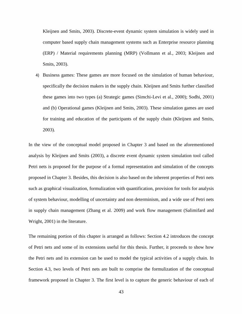
4) Business games: These games are more focused on the simulation of human behaviour,
specifically the decision makers in the supply chain. Kleijnen and Smits further classified
these games into two types (a) Strategic games (Simchi-Levi et al., 2000); Sodhi, 2001)
and (b) Operational games (Kleijnen and Smits, 2003). These simulation games are used
for training and education of the participants of the supply chain (Kleijnen and Smits,
2003).
In the view of the conceptual model proposed in Chapter 3 and based on the aforementioned
analysis by Kleijnen and Smits (2003), a discrete event dynamic system simulation tool called
Petri nets is proposed for the purpose of a formal representation and simulation of the concepts
proposed in Chapter 3. Besides, this decision is also based on the inherent properties of Petri nets
such as graphical visualization, formulization with quantification, provision for tools for analysis
of system behaviour, modelling of uncertainty and non determinism, and a wide use of Petri nets
in supply chain management (Zhang et al. 2009) and work flow management (Salimifard and
Wright, 2001) in the literature.
The remaining portion of this chapter is arranged as follows: Section 4.2 introduces the concept
of Petri nets and some of its extensions useful for this thesis. Further, it proceeds to show how
the Petri nets and its extension can be used to model the typical activities of a supply chain. In
Section 4.3, two levels of Petri nets are built to comprise the formulization of the conceptual
framework proposed in Chapter 3. The first level is to capture the generic behaviour of each of

44
the members in a supply chain network and the second level is at a higher level to capture the
interactions among the members in a supply chain network. The second level aggregates the
Petri nets built in the first level. Section 4.4 concludes the chapter.
4.2 Background and Literature review
4.2.1 Classical Petri nets
Classical Petri nets also sometimes referred to as basic Petri nets were first introduced by Carl
Adam Petri through his PhD dissertation. There are four major elements in classical Petri net
modelling namely places, transition, arc and tokens (Murata, 1989).
1) Places (p): These are type of nodes in the Petri net. Places in the Petri net are denoted by
circles. Places represent events, conditions or resources in modelling.
2) Transitions (t): These are the second type of nodes in the Petri net. These are drawn by
rectangular boxes or bars. Transitions are used to represent events, transformation
processes, etc.
3) Tokens: A token is represented as a dot. Tokens are used to show the presence of
physical objects or informational object and can also act as indicators of state or a
condition of place. The number of tokens at a place is used to find the state of Petri net.
The state of Petri net also called as marking is represented by the distribution of tokens
over places. The marking of a Petri net is vector, and length of the vector is equal to the
number of places in the Petri net.
4) Arcs: Arcs are directed arrows connecting two different types of nodes in the Petri net
(i.e. places and transitions). Arcs cannot be used to connect any two places or two
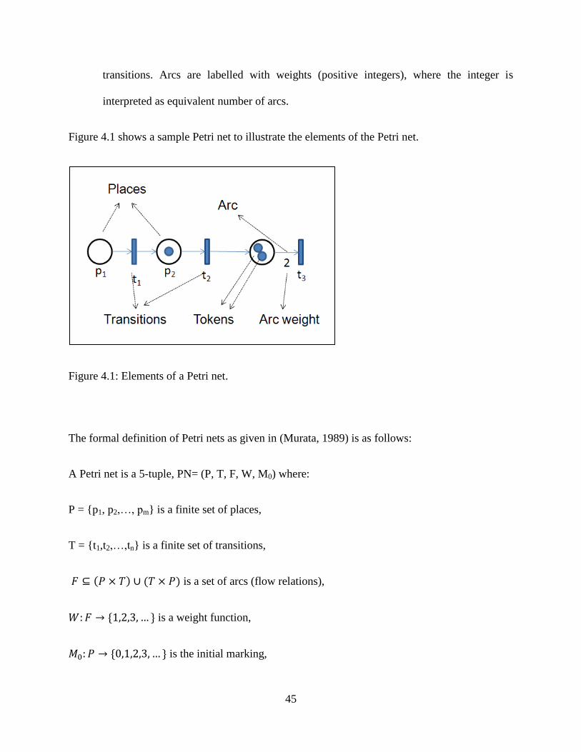
45
transitions. Arcs are labelled with weights (positive integers), where the integer is
interpreted as equivalent number of arcs.
Figure 4.1 shows a sample Petri net to illustrate the elements of the Petri net.
Figure 4.1: Elements of a Petri net.
The formal definition of Petri nets as given in (Murata, 1989) is as follows:
A Petri net is a 5-tuple, PN= (P, T, F, W, M0) where:
P = {p1, p2,…, pm} is a finite set of places,
T = {t1,t2,…,tn} is a finite set of transitions,
is a set of arcs (flow relations),
is a weight function,
is the initial marking,
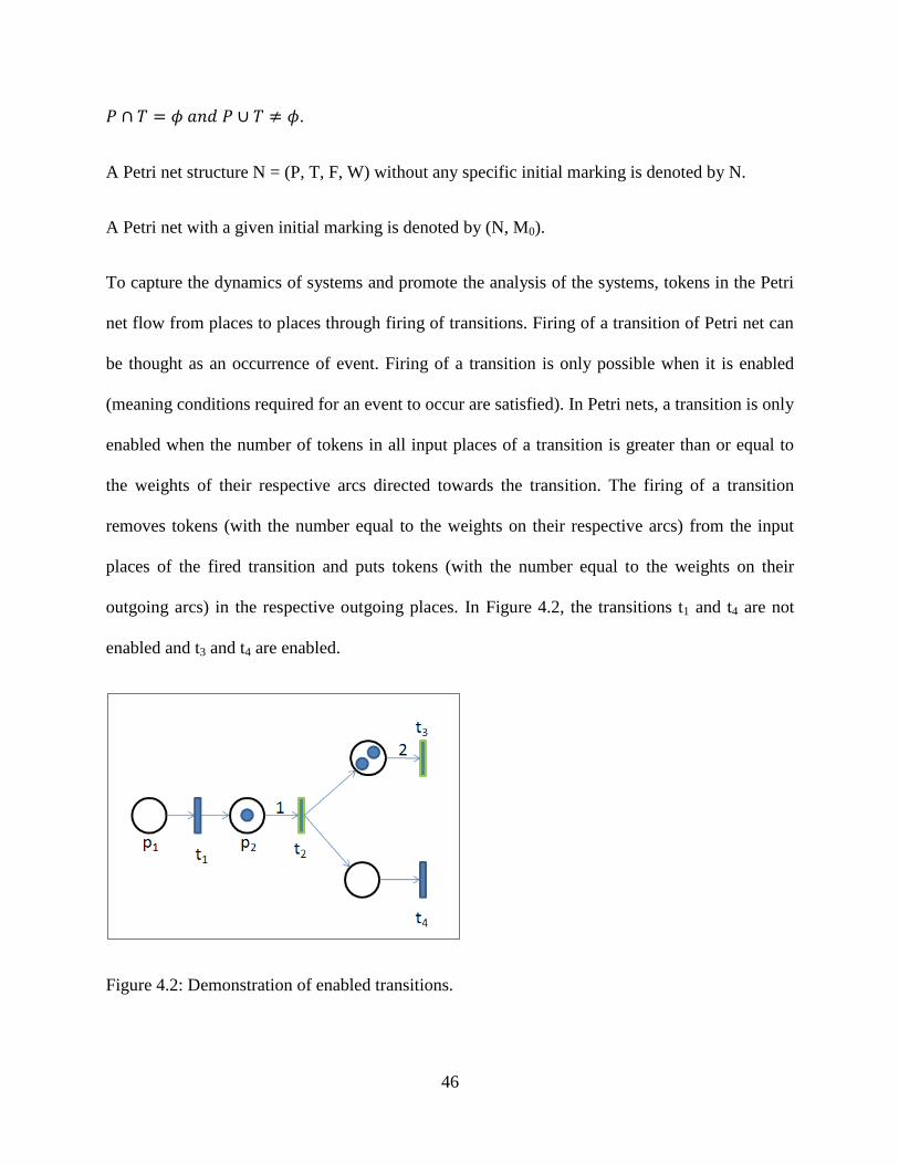
46
.
A Petri net structure N = (P, T, F, W) without any specific initial marking is denoted by N.
A Petri net with a given initial marking is denoted by (N, M0).
To capture the dynamics of systems and promote the analysis of the systems, tokens in the Petri
net flow from places to places through firing of transitions. Firing of a transition of Petri net can
be thought as an occurrence of event. Firing of a transition is only possible when it is enabled
(meaning conditions required for an event to occur are satisfied). In Petri nets, a transition is only
enabled when the number of tokens in all input places of a transition is greater than or equal to
the weights of their respective arcs directed towards the transition. The firing of a transition
removes tokens (with the number equal to the weights on their respective arcs) from the input
places of the fired transition and puts tokens (with the number equal to the weights on their
outgoing arcs) in the respective outgoing places. In Figure 4.2, the transitions t1 and t4 are not
enabled and t3 and t4 are enabled.
Figure 4.2: Demonstration of enabled transitions.
47
Although basic Petri nets, classified as low level Petri nets (Vasilis et.al , 1998), they have been
successfully implemented in many applications such as performance evaluation and
communication protocols (the reader is directed to Murata(1989) for a complete list of
applications), some drawbacks of the basic Petri Nets have been addressed in the literature, and
many extensions have been proposed to improve the basic Petri nets, resulting in various
extensions. Common drawbacks of the low level Petri nets or basic Petri nets are listed as
follows:
1) Inability to distinguish the tokens, hence lacking simultaneous representation of various
objects and their attributes.
2) Complex structures and lack of compactness.
3) Lack of control over firing of the transition and do not capture time aspect.
Following these backlogs many extensions have been made to Petri nets. The evolution of these
Petri nets is well described by (He and Murata, 2005), and they classified the evolution of Petri
Nets into the following four generations:
1) Low Level Petri nets (First generation): for modeling system control (Reisig, 1985):
2) High Level Petri nets (Second Generation): for describing both system data and control
(Jensen and Rozenberg, 1991).
3) Hierarchical Petri nets (Third-generation): for abstracting system structures (He and Lee,
1991; He, 1996; Jensen, 1992).
4) Object-oriented Petri nets (Fourth-generation): for supporting modern system
development approaches (Agha, 2001).

48
There are some other developments aiming to reduce the complexity of Petri nets, e.g., Zhang et
al. (2000), He (2008), etc. In work of Zhang et al. (2000), a generic or template Petri nets is
proposed, which is related to individual applications. In He (2008), the function-behaviour-
structure concept (Lin and Zhang, 2004; Zhang et al., 2005) is applied to Petri Nets, leading to
three related Petri nets: the principle Petri net, structure Petri net, behaviour Petri net.
The comparison of some of these extensions is well described by Vasilis et al. (1998) based on
various criteria. For the purpose of the current work, this thesis only discuss three extensions of
Petri net, which are considered to be sufficient for developing a tool to implement the proposed
framework of Chapter 3.
4.2.2 Extensions of Petri net
Coloured Petri nets (Jensen, 1981, 1990, 1995):
The major contribution of this extension is that it allows distinguishing the tokens (using colours)
in a place and allows asserting attributes to the objects. Hence, they carry a more descriptive
power than the classical Petri nets. Having one place to carry different types of tokens drastically
reduces the number of places in the Petri net and thus the structural complexity of the net. The
use of coloured Petri nets in this work is demonstrated through a sample Petri net shown in
Figure 4.3, which consists of two places named “Products ordered” and “Orders accepted”. The
former place carries two tokens of different colours representing two orders of different products
(namely Product A and Product B). Besides, attributes such as order number can be asserted to
the tokens as shown in Figure 4.3. There are two variables in the Petri namely „x‟ and „i'. „x‟
carries the information of the product name and ‟i' is an integer that carries information about the
order number. An order for a product received is denoted by a coloured token in place named

49
“Product orders” and these order are accepted (event taking place) the tokens are moved to the
place named “Accepted orders”. Hence, from Figure 4.3, it can be observed that coloured Petri
nets has the provision to distinguish the tokens and additional information can be carried by the
tokens through the net.
Figure 4.3: Differentiating tokens using Coloured Petri Nets.
Apart from this coloured Petri nets are embedded with the capability to express selection of
firing of transitions based on pre-specified conditions and further controlling the removal of the
number and type of tokens from the input places and putting the resultant tokens in output
places. Jensen (1983 and 1986) proposes arc expressions and guards that could be used for this
purpose. These capabilities of the coloured Petri nets are later demonstrated in the later sections
of this chapter.
Timed Petri nets:
“In timed Petri nets, each transition takes a 'real time' to fire; i.e., there is a 'firing time'
associated with each transition of a net which determines the duration of transition's firings”
(Zuberek and Kubiak, 1999). Time Petri nets facilitate to have the information of time in the
Petri net models. This enhances the capability to obtain performance measures related to time

50
such as waiting times, delays, throughput times and other efficiencies (Jensen, 2007). To
incorporate time in the Petri nets, Jensen (2007) introduced the concept of time stamp through
the software called Coloured Petri net tools. The time stamp tells us the time at which the token
is ready to be used; i.e., the time at which it can be removed from the place by an occurring
transition (Jensen, 2007). Besides, it gives the user the power to model transitions that take place
periodically. For example, suppose the employees of a manufacturing company are paid monthly
salaries and the flow of money occurs once in a month (i.e. the event of payment). This can be
modelled using the timed Petri net, as shown in Figure 4.4.
Figure 4.4 Use of Timed Petri net to model periodic events.
Hierarchical Petri nets:
Hierarchical Petri nets are introduced to solve the complexity problem in the Petri nets. The two
different mechanisms (Wang and Wei, 2009) proposed in literature for the building of hierarchy
in the Petri nets are:
1. Transition refinement and
2. Subnet abstraction

51
The technique of transition refinement is used for the top-down system development processes,
where a transition is substituted with a subnet containing the detailed tasks of the transition in the
Petri net (Wang and Wei, 2009). In contrast to this, subnet abstraction is used for bottom-up
system development process, where a set of tasks are removed in the form of subnet and replaced
by a single transition (Wang and Wei, 2009). Humber et al. (1991) demonstrated how coloured
Petri nets can be extended to exhibit the property of hierarchy. The hierarchy in Coloured Petri
nets can be achieved in by one of the following methods:
a) Substitution Transitions: The details of the substitution transition are stored in a separate
page called the subpage, to offer a simple view of the primary Petri net. The substitution
transition called the super node and the page containing this transition is called the super
page with respects their subpage.
b) Substitution Places: This method is similar to the substitution of transition except that
places are used for substitution instead of transitions.
c) Invocation transitions: In this method, the transitions are not substitutions. Hence, they
can concurrently operate with other page instances in the model.
d) Place fusion: Conceptually folding of set of places in the Petri net into a single place.
e) Transition fusion: Conceptually folding of set of transitions in the Petri net into a single
transition.
The use of hierarchical Petri nets and their role in the representation of a supply chain network is
illustrated in the next section.

52
4.3 Petri nets for a Supply Chain Network
In this section, the concepts of Petri nets introduced in Section 4.2 will be used to realize the
conceptual framework of a supply chain network proposed in Chapter 3. It is noted that the
proposed conceptual framework has two levels. The first level is an overall view to display the
health statuses of all firms in a supply chain network. To capture and represent information and
knowledge at this level, a Petri net called primary Petri net is constructed. The second level is the
health of each of the members in the supply chain network, represented by a dot on the node of a
supply chain network. To capture this semantics, a notion called “subnet” in Petri net is proposed
herein. A subnet of a firm is a Petri net used to evaluate the status of the firm and to feed the
primary Petri net with the information of each of the members in a supply chain network. This
idea can be implemented with hierarchical Petri nets discussed in the previous section.
Furthermore, with the hierarchical Petri nets, the primary Petri net can be constructed in one of
the following alternatives:
Alternative 1:
Places in the primary Petri net are used to represent firms, and their status is identified by the
tokens present in these places. The tokens are fed by the subnets, associated with each of the
firms. Figure 4.5 shows four firms A, B, C, D, represented by places (circular nodes), and each
of them is connected with their respective subnets to update their status. This alternative is best
when the number of firms (equivalent to the number of places in Petri net) in a supply chain
network is not too large. Although the Petri net works for a large number of places, the trade-off
would be taken in terms of visual clarity (i.e., the more number of nodes, the less is the visual
clarity of the Petri net).
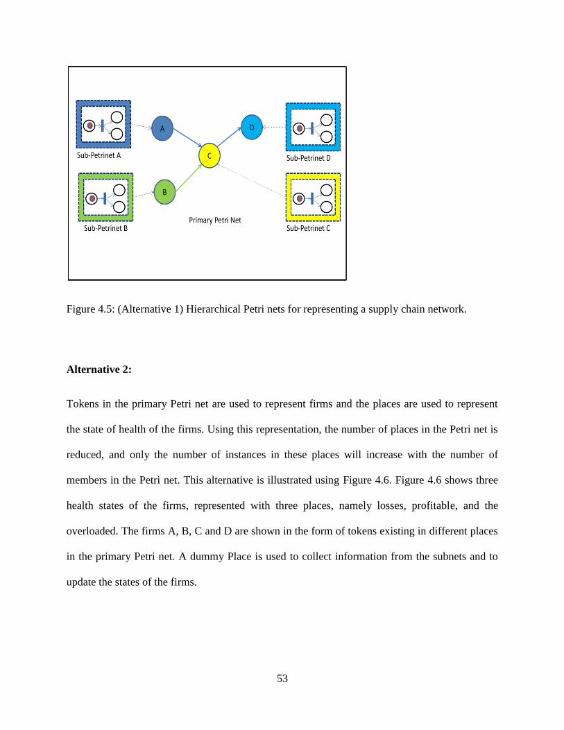
53
Figure 4.5: (Alternative 1) Hierarchical Petri nets for representing a supply chain network.
Alternative 2:
Tokens in the primary Petri net are used to represent firms and the places are used to represent
the state of health of the firms. Using this representation, the number of places in the Petri net is
reduced, and only the number of instances in these places will increase with the number of
members in the Petri net. This alternative is illustrated using Figure 4.6. Figure 4.6 shows three
health states of the firms, represented with three places, namely losses, profitable, and the
overloaded. The firms A, B, C and D are shown in the form of tokens existing in different places
in the primary Petri net. A dummy Place is used to collect information from the subnets and to
update the states of the firms.

54
Figure 4.6: (Alternative 2) Hierarchical Petri nets for representing a supply chain network.
Following the construction of the primary Petri net, the reminder of this section will focus on the
construction of the subnets for members in a supply chain network. For this purpose, the typical
operations of members in a supply chain network are identified. A classification is made among
the participating firms of the supply chain network based on their types of operations. The first
type is the manufacturing (i.e., gathering components for a product and assembling them), and
the other is the service firm (which either transfers the input to the consecutive member in the
supply chain or offers support such as transportation arrangement, legal documentation, and so
on). Although the operations performed are different in nature, a general work flow might be
assumed for all the firms. The general work flow for a supply chain network member defined in
this thesis is as follows:
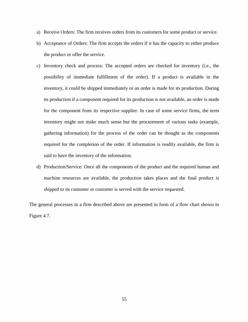
55
a) Receive Orders: The firm receives orders from its customers for some product or service.
b) Acceptance of Orders: The firm accepts the orders if it has the capacity to either produce
the product or offer the service.
c) Inventory check and process: The accepted orders are checked for inventory (i.e., the
possibility of immediate fulfillment of the order). If a product is available in the
inventory, it could be shipped immediately or an order is made for its production. During
its production if a component required for its production is not available, an order is made
for the component from its respective supplier. In case of some service firms, the term
inventory might not make much sense but the procurement of various tasks (example,
gathering information) for the process of the order can be thought as the components
required for the completion of the order. If information is readily available, the firm is
said to have the inventory of the information.
d) Production/Service: Once all the components of the product and the required human and
machine resources are available, the production takes places and the final product is
shipped to its customer or customer is served with the service requested.
The general processes in a firm described above are presented in form of a flow chart shown in
Figure 4.7.
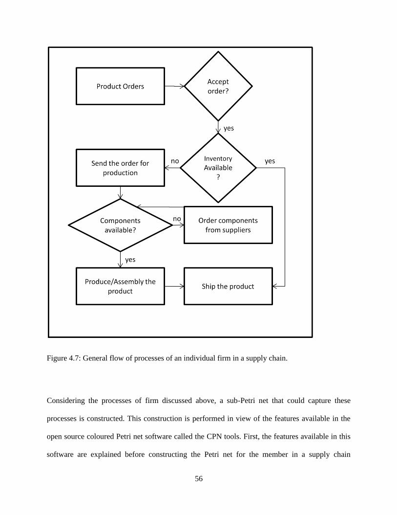
56
Figure 4.7: General flow of processes of an individual firm in a supply chain.
Considering the processes of firm discussed above, a sub-Petri net that could capture these
processes is constructed. This construction is performed in view of the features available in the
open source coloured Petri net software called the CPN tools. First, the features available in this
software are explained before constructing the Petri net for the member in a supply chain
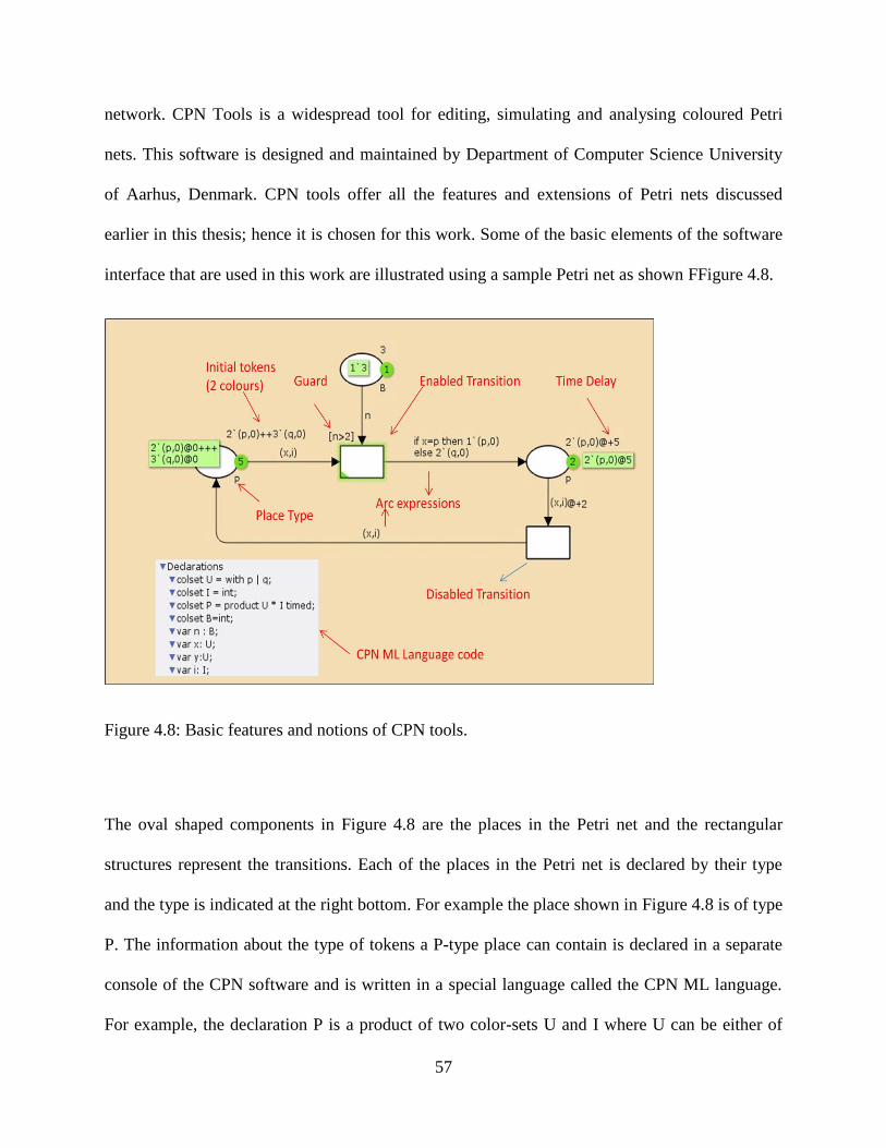
57
network. CPN Tools is a widespread tool for editing, simulating and analysing coloured Petri
nets. This software is designed and maintained by Department of Computer Science University
of Aarhus, Denmark. CPN tools offer all the features and extensions of Petri nets discussed
earlier in this thesis; hence it is chosen for this work. Some of the basic elements of the software
interface that are used in this work are illustrated using a sample Petri net as shown FFigure 4.8.
Figure 4.8: Basic features and notions of CPN tools.
The oval shaped components in Figure 4.8 are the places in the Petri net and the rectangular
structures represent the transitions. Each of the places in the Petri net is declared by their type
and the type is indicated at the right bottom. For example the place shown in Figure 4.8 is of type
P. The information about the type of tokens a P-type place can contain is declared in a separate
console of the CPN software and is written in a special language called the CPN ML language.
For example, the declaration P is a product of two color-sets U and I where U can be either of

58
color „p‟ or color „q‟ and I is an integer. The declaration contains the description of variables
such that „x‟ represents either of the colors „p‟ or „q‟ of the colour set U. An initial number of
tokens in a place can be specified on its top right hand corner of the place. For example in Figure
4.8, the left most place of type P is initiated with two (p, 0) coloured tokens and three (q, 0) type
coloured tokens and the number 5 in the green bubble indicates the total number of tokens in the
place.
Arc expressions are used to specify the type and number of tokens to be removed from the place
and the type and number of tokens to be placed in output place. Further, control statements can
be used as arc expressions to control the flow of token numbers. For example, the control
statement in Figure 4.8 shows that if the input to the transition is a p coloured token i.e. x=p),
one token of the similar colour is placed in the output place or else two tokens of q coloured are
placed in the output place of the transition. In addition, to the control provided by the arc
expressions, CPN tools provide an extra feature called the guard that could place additional
constraints on the firing of transition. If the guard evaluates to be true only, a transition is
enabled given all other arc conditions satisfied. In the above example, the guard is true if the
value of n is greater than 2, since the value of n is 3, the transition is enabled. The enabled
transitions are highlighted by green glowing shade while disabled transitions remain without any
shade. Time is added to Petri net by declaring the place type with the command timed in the
declaration console. Time delays can be added using “@ + time delay expression” to the tokens
at the places. In Figure 4.8, a time delay of 5 is added to the tokens in the rightmost corner place.
This means that these tokens will only be available for the transition at 5 time units from the start
of the simulation because of this the transition following this place is not enabled as shown in
Figure 4.8. It is to be noted that the snapshot is taken at start of simulation, hence time=0 units.
59
In addition to the initial time delays stamps of the tokens, time delay expressions can also be
added to the arc expression. For example, a time delay of 2 units is added to the input arc of right
bottom transition in Figure 4.8. This means that every token flow through this arc incurs an
additional time delay of two units.
The features available in the CPN tools are used to form a generic Petri net for the processes of a
supply chain firm. Without loss of generality, a Petri net for a firm to produce two different
products (extendable to any number of products) is constructed. The Petri net also considers that
two products (say Product X and Product Y) utilize two different components Component A and
Component B supplied by external suppliers. Further, the number of components used in making
of a product is varied; i.e. Product X requires two quantities of component A and one quantity of
component B, while Product Y requires three quantities of component A and two quantities of
component B.

60
Figure 4.9: Petri net for the member in a supply chain network.
Demand for product X or product Y is generated in the place named “Demand” as shown in
Figure 4.9. The initial tokens present in this place show the demand is for one of product X and 2
products of Y. The transition “Orders accepted” is enabled as there exist tokens in the place
“Capacity” representing the capacity(say production capacity) of the firm to accept orders. Once
the order is accepted orders move to “Order in process” state and a token is also removed from
the capacity of the firm. Here if the inventory is available the product is shipped (transition ship
is fired) or else the component is moved for the production process. Depending on the product
ordered, the required numbers of tokens (components of a product) are placed in places ComA
representing the quantity of Component A required and ComB denoting for Component B. If the

61
components are available in their respective inventories places InvA and InvB then they are
moved for the assembly or the production of product else orders are placed for the components.
The inventories are refilled as the components are supplied from the supplier places SupA and
SupB. When all the components required for the production of the product are in position, the
assembly takes place moved to inventory which is further moved to shipment. After each
shipment is made the capacity of the firm is increased by one token thus maintaining the orders
that can be accepted. The expenditures made through the procurement of components A and B
are stored in places ExpA and ExpB, respectively. The production cost and the revenue made by
the firm directed towards assessment transition and the status of the company are determined.
This status information is sent to the primary Petri net as explained at the beginning of this
section.
4.4 Summary
This chapter presented a tool to implement the conceptual framework of the supply chain
network proposed in Chapter 3. This tool is based on Petri nets. The primary Petri net tailored in
this chapter facilitates to view the supply chain network at a holistic level and can be used to
monitor the change of states of the firms in a supply chain network. The subnets of the individual
firms maintain the statistics of the firm‟s material supply, capacity of production, inventory
levels, throughput time, production costs and product revenues and perform the dynamic
updating of the firm‟s health in the network. Embedding these Petri nets with time and
simulating a disruption at one firm, propagation of the disruption can be observed in the primary
network. This simulation will help a firm to release the possible effect of the disruption in the
supply chain network and the time for the effect to propagate to it. The next chapter of this thesis

62
takes up to demonstrate similar simulations with several case studies related to the supply chain
network.
63
Chapter 5 Case Studies and Applications
5.1 Introduction
It is evident that supply chain networks play a major role in society. They act as a backbone in
supporting the economics of various communities throughout their span. A supply chain network
not only supports the supply of commodities and services but also provides the economic
sustainability to society in the form of jobs. Given this strong connection of it with well being of
a community, the collapse of a supply chain network (or even a portion of it) could be a
devastating effect on the lives of the people who depend on it for living. Hence, it should be of
government‟s interest to regulate the structure and behaviour of the supply chain network to
avoid such failure. Although government intervention has been noticed in the recent past in lieu
of financial crisis at the first instance, such intervention is only after the considerable damage
taking place in the supply chain system. The bail-out package from the US government during
the 2008 financial crisis has clearly indicated that government‟s intervention can be categorized
as being mostly reactive (taking a necessary action after considerable damage has occurred) as
opposed to being proactive (taking a necessary action before considerable damage is predicted).
The framework proposed in this thesis aims to serve as a supporting tool for governments or
other public interest organizations responsible for well being of a supply chain network. In the
remainder of this thesis, the term „Regulatory Body‟ is used to refer to such an organization
(either appointed by a government or chosen by members of a supply chain network) which acts

64
as a vigilante of the supply chain network. The main responsibility of such regulatory body is to
collect the information of the statuses of members of a supply chain network, analyze possible
and occurring disruptions, and provide early indication of possible spreads of disruptions to
relevant members of the supply chain network. This would help members of the network, who
would be affected due to disruptions in the network, to prepare ahead of time. In other words,
regulatory body is the committee that monitors and maintains the framework proposed in this
thesis.
This thesis work also assumes that members in a supply chain network share their health status
and information of disruptions with a regulatory body. This chapter will demonstrate how the
proposed framework (predictive in nature) could be implemented to foresee the danger of
collapse of an entire supply chain network with help of a sample case study. The first case study
relates to the supply chain network centered around the American automobile manufacturing
industry, specific to the recent bankruptcy of the American big three companies and its effects on
society. It is to be noted that the case study is built from reading newspaper articles and blogs
which are placed separately in the reference section at the end of this thesis.
5.2 Case Study: ‘Big Three’ Automobile Manufacturers in the United States.
In the year 2008, the three major American automobile manufacturers (General Motors, Ford and
Chrysler) =had to request $50 billion dollars from the US government as part of the bailout
package. The three companies gradually recovered with this support from the government and
market forces further arising due to the recent call-backs of vehicles by their Japanese
competitor, Toyota.
65
The roots of the crisis did not take place overnight. Some of the causes of the crisis of the Big-
Three companies are: production of fuel inefficient vehicles; shift of focus on the pick truck
business in anticipation of larger profit margins regardless of the fuel price sensitivity and
climate changes. In contrast, the Japanese car manufacturers, who focused on producing fuel
efficient cars, captured most car markets during this time.
In the supply chain literature, only a few studies have considered the interdependency of the
Japanese car companies and the American car companies through their common supplier base.
Only during the big three crisis did this interdependency come to picture. Honda, the Japanese
automobile giant, had requested the United States government to support the American „big
three‟ to avoid the spreading of the disruptions to the healthy manufactures of the automobile
industry. The problems of the „big three‟ were only viewed as some competitive advantage
during the period 2000-2007, and the common supplier base interdependency was overlooked.
The interdependency between the competitors is the common supplier to these companies. Both
the American and Japanese labels have the same supplier base. If the supplier base gets affected
due to the troubles of the American automobile companies, the suppliers in the common supplier
base would not be able to supply materials to the Japanese companies and thus this would result
in a problem for the Japanese companies while initially the problem only occurred to the
American “Big Three”. A major impact was felt on the community as well. Hundreds of
thousands of jobs were lost due to the direct and indirect effect of the collapse of the American
„Big Three‟ companies. This further had a catastrophic impact on the economic activities in other
businesses (e.g., retail, etc).
66
The solution principle to such a problem is to find a way to predict these effects in the
automobile supply chain and to prepare for it, which has been presented in Chapter 3. In Chapter
4, such a solution principle was further described in detail, which has led to a tool for regulatory
body to take proactive actions in time. In the following, the use of this tool for the “Big Three”
problem will be presented. To demonstrate the use of the tool, a supply chain network is to be
constructed. Recreating the automobile supply chain network is out of the scope of this thesis as
such a network is extremely widespread, involves a huge number of members and demands a
considerable amount of effort on data collection and processing. So, a hypothetical case is
constructed in this study. An additional assumption is made that each member of the network
will keep regulatory body informed of their statuses.
With the hypothetical case, this thesis will show how the information generated by the Petri net
model proposed in this thesis can be used to predict and avoid collapses that occurred in the
aforementioned case of the „Big Three‟. The case assumes a supply chain network structure with
two leading automobile manufacturers (Company A and Company B) participating in the
proposed framework who depend on common suppliers (Supplier 1 for component 1 and
Supplier 2 for component 2). The representation of the network is shown in Figure 5.1.
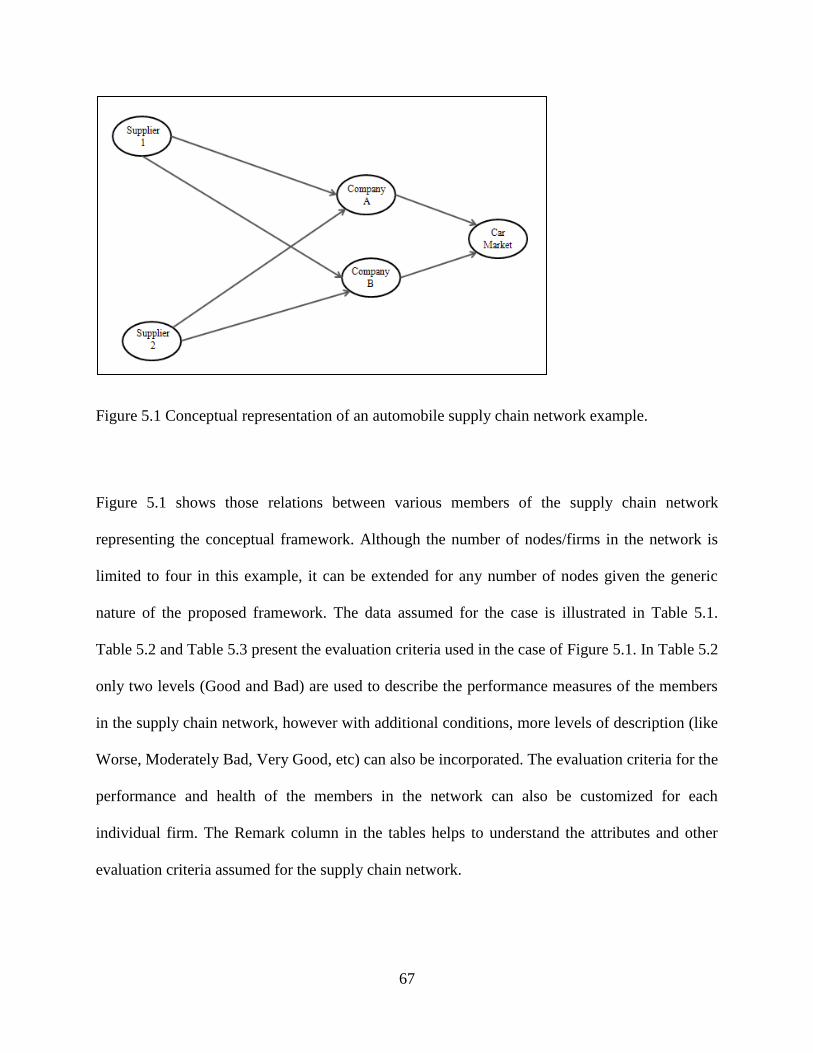
67
Figure 5.1 Conceptual representation of an automobile supply chain network example.
Figure 5.1 shows those relations between various members of the supply chain network
representing the conceptual framework. Although the number of nodes/firms in the network is
limited to four in this example, it can be extended for any number of nodes given the generic
nature of the proposed framework. The data assumed for the case is illustrated in Table 5.1.
Table 5.2 and Table 5.3 present the evaluation criteria used in the case of Figure 5.1. In Table 5.2
only two levels (Good and Bad) are used to describe the performance measures of the members
in the supply chain network, however with additional conditions, more levels of description (like
Worse, Moderately Bad, Very Good, etc) can also be incorporated. The evaluation criteria for the
performance and health of the members in the network can also be customized for each
individual firm. The Remark column in the tables helps to understand the attributes and other
evaluation criteria assumed for the supply chain network.
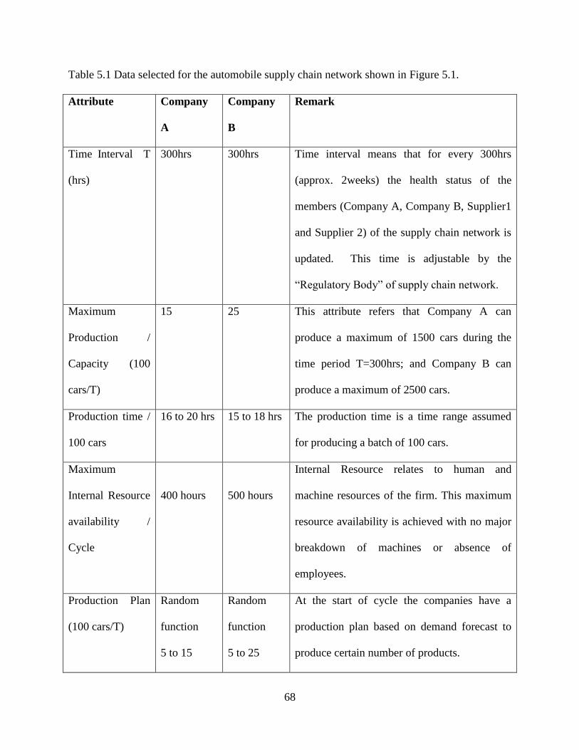
68
Table 5.1 Data selected for the automobile supply chain network shown in Figure 5.1.
Attribute Company
A
Company
B
Remark
Time Interval T
(hrs)
300hrs 300hrs Time interval means that for every 300hrs
(approx. 2weeks) the health status of the
members (Company A, Company B, Supplier1
and Supplier 2) of the supply chain network is
updated. This time is adjustable by the
“Regulatory Body” of supply chain network.
Maximum
Production /
Capacity (100
cars/T)
15 25 This attribute refers that Company A can
produce a maximum of 1500 cars during the
time period T=300hrs; and Company B can
produce a maximum of 2500 cars.
Production time /
100 cars
16 to 20 hrs 15 to 18 hrs The production time is a time range assumed
for producing a batch of 100 cars.
Maximum
Internal Resource
availability /
Cycle
400 hours
500 hours
Internal Resource relates to human and
machine resources of the firm. This maximum
resource availability is achieved with no major
breakdown of machines or absence of
employees.
Production Plan
(100 cars/T)
Random
function
5 to 15
Random
function
5 to 25
At the start of cycle the companies have a
production plan based on demand forecast to
produce certain number of products.
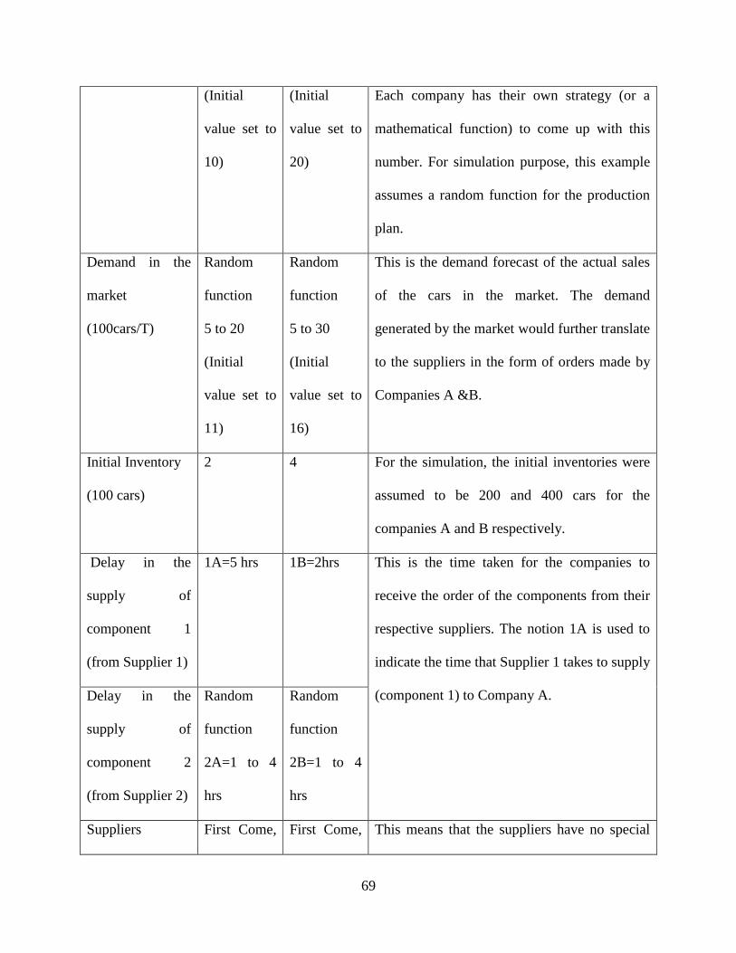
69
(Initial
value set to
10)
(Initial
value set to
20)
Each company has their own strategy (or a
mathematical function) to come up with this
number. For simulation purpose, this example
assumes a random function for the production
plan.
Demand in the
market
(100cars/T)
Random
function
5 to 20
(Initial
value set to
11)
Random
function
5 to 30
(Initial
value set to
16)
This is the demand forecast of the actual sales
of the cars in the market. The demand
generated by the market would further translate
to the suppliers in the form of orders made by
Companies A &B.
Initial Inventory
(100 cars)
2 4 For the simulation, the initial inventories were
assumed to be 200 and 400 cars for the
companies A and B respectively.
Delay in the
supply of
component 1
(from Supplier 1)
1A=5 hrs
1B=2hrs
This is the time taken for the companies to
receive the order of the components from their
respective suppliers. The notion 1A is used to
indicate the time that Supplier 1 takes to supply
(component 1) to Company A. Delay in the
supply of
component 2
(from Supplier 2)
Random
function
2A=1 to 4
hrs
Random
function
2B=1 to 4
hrs
Suppliers First Come, First Come, This means that the suppliers have no special

70
Preference first serve. first serves. preferences for their customers (Company A
and B) and the orders are served based on first-
come–first-served basis.

71
Table 5.2 Evaluation criteria for key Supply Chain Performance Measures.
Performance
Measure
Evaluation criteria of the
performance measure
Remark
Company A Company B
Utilization (of
production capacity)
(j1) (100 cars)
Good if j1 <4
else Bad
Good if j1 <8
else Bad
It is the difference between the
maximum production capacity and
the actual production in a given
time period. E.g. If a car
manufacturing company makes
only 300 cars when it has the
capability of making 500 cars then
j1= (500-300)/100=2.
Unsatisfied demand
(j2) (100 cars)
Good if j2 < 2
or else Bad
Good if j2 < 3
or else Bad
This figure denotes the lost sales
irrespective of the cause.
Inventory level (j3)
(100 cars)
Good if j3 < 3
or else Bad
Good if j3 < 4
or else Bad
Inventory level at the end of each
cycle (T=300hrs).
Products sold (j4) (100
cars)
Good if j4 > 10
or else Bad
Good if j4 > 16
or else Bad
Products sold during the time
interval (T)
Relationship with
Good if j5 > 7
or else Bad
Good if j5 > 10
or else Bad
This measures the relationship
between the supplier and
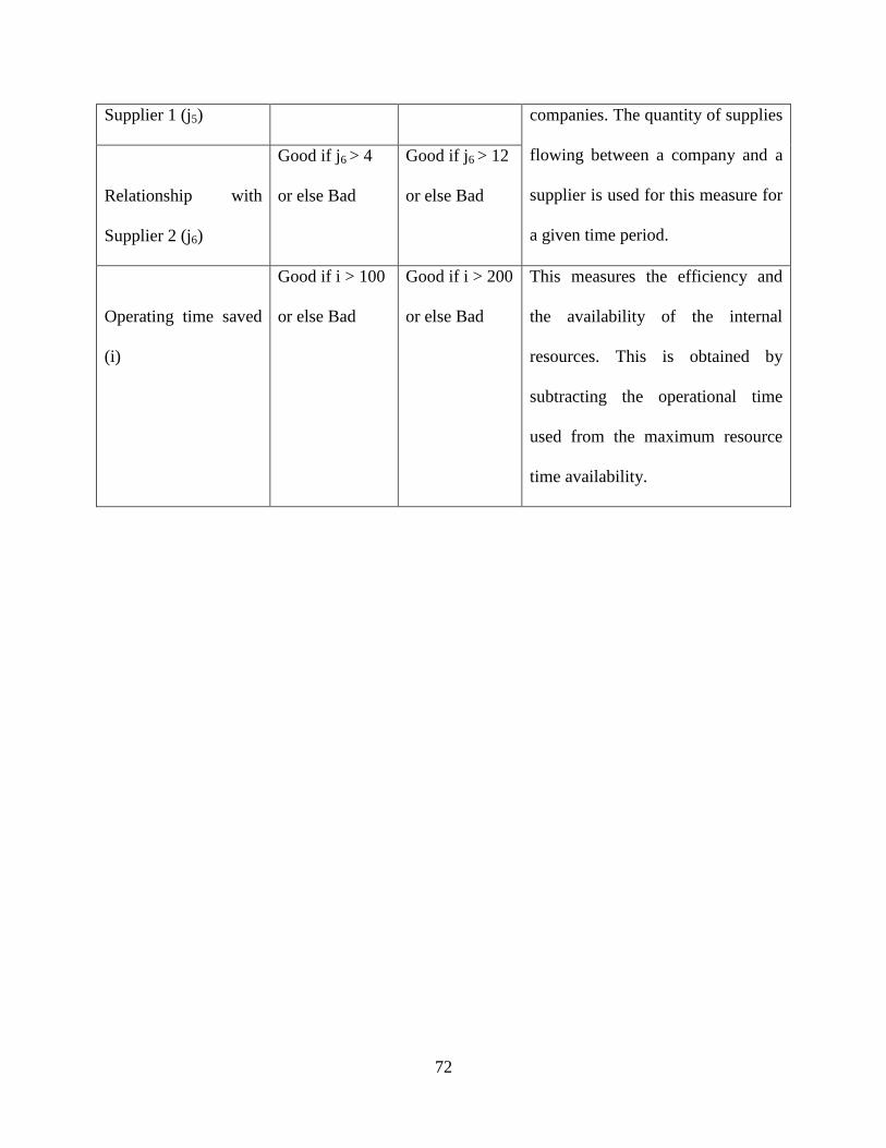
72
Supplier 1 (j5) companies. The quantity of supplies
flowing between a company and a
supplier is used for this measure for
a given time period.
Relationship with
Supplier 2 (j6)
Good if j6 > 4
or else Bad
Good if j6 > 12
or else Bad
Operating time saved
(i)
Good if i > 100
or else Bad
Good if i > 200
or else Bad
This measures the efficiency and
the availability of the internal
resources. This is obtained by
subtracting the operational time
used from the maximum resource
time availability.
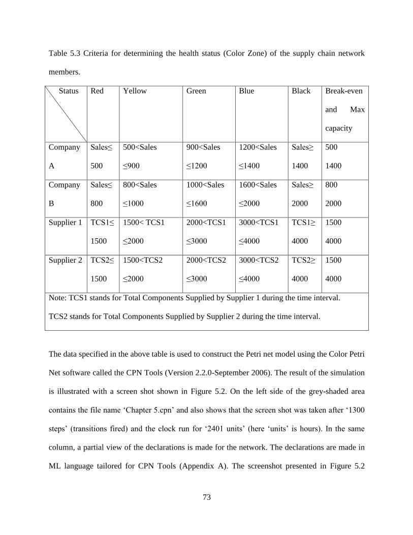
73
Table 5.3 Criteria for determining the health status (Color Zone) of the supply chain network
members.
Status Red Yellow Green Blue Black Break-even
and Max
capacity
Company
A
Sales≤
500
500<Sales
≤900
900<Sales
≤1200
1200<Sales
≤1400
Sales≥
1400
500
1400
Company
B
Sales≤
800
800<Sales
≤1000
1000<Sales
≤1600
1600<Sales
≤2000
Sales≥
2000
800
2000
Supplier 1 TCS1≤
1500
1500< TCS1
≤2000
2000<TCS1
≤3000
3000<TCS1
≤4000
TCS1≥
4000
1500
4000
Supplier 2 TCS2≤
1500
1500<TCS2
≤2000
2000<TCS2
≤3000
3000<TCS2
≤4000
TCS2≥
4000
1500
4000
Note: TCS1 stands for Total Components Supplied by Supplier 1 during the time interval.
TCS2 stands for Total Components Supplied by Supplier 2 during the time interval.
The data specified in the above table is used to construct the Petri net model using the Color Petri
Net software called the CPN Tools (Version 2.2.0-September 2006). The result of the simulation
is illustrated with a screen shot shown in Figure 5.2. On the left side of the grey-shaded area
contains the file name „Chapter 5.cpn‟ and also shows that the screen shot was taken after „1300
steps‟ (transitions fired) and the clock run for „2401 units‟ (here „units‟ is hours). In the same
column, a partial view of the declarations is made for the network. The declarations are made in
ML language tailored for CPN Tools (Appendix A). The screenshot presented in Figure 5.2

74
contains Binder 0 with various pages/tabs. These tabs contain Petri nets that capture different
aspects of the supply chain network. The purpose of each tab and their respective Petri nets are
presented in Table 5.4. The screen shots of all the Petri net tabs are presented in Appendix A for
completeness and a file (in .cpn format) of this model is included in the CD attached with this
thesis.
Figure 5.2: Petri net model of a sample run of an automotive industry example.

75
Table 5.4 Pages of the Petri net model of an automobile supply chain network.
Tab/ Page Name Purpose Pages with
immediate
Hierarchy.
Company A Contains the Petri net to capture the supply chain
activity of Company A.
Supply 1A, Supply
2A, Status A.
Company B Contains the Petri net to capture the supply chain
activity of Company B.
Supply 1B, Supply
2B, Status B.
Supply 1A Contains the Petri net to capture all the supply
from Supplier 1 to Company A.
Company A,
Suppliers Evaluation.
Supply 2A Contains the Petri net to capture all the supply
from Supplier 2 to Company A.
Company A,
Suppliers Evaluation.
Supply 1B Contains the Petri net to capture all the supply
from Supplier 1 to Company B.
Company B,
Suppliers Evaluation.
Supply 2B Contains the Petri net to capture all the supply
from Supplier 2 to Company B.
Company B,
Suppliers Evaluation.
Status A Contains a Petri net that gathers all the
performance measures data (see table 5.2) of a
Company at the end of every time cycle(T) and
sends the same data to Detail Status page for the
evaluation of the performance measures and the
assignment of Health Status(Color zone). This
Petri net also updates the Company Petri net
Company A, Detail
Status A.
Status B Company B, Detail
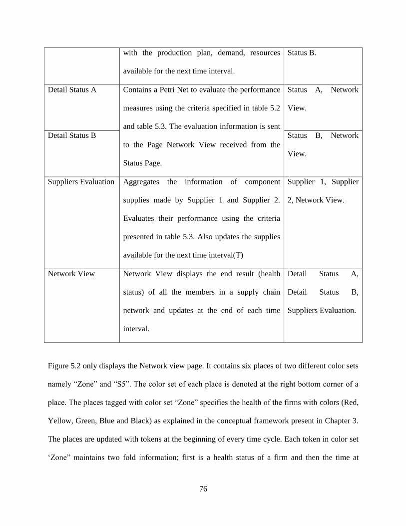
76
with the production plan, demand, resources
available for the next time interval.
Status B.
Detail Status A Contains a Petri Net to evaluate the performance
measures using the criteria specified in table 5.2
and table 5.3. The evaluation information is sent
to the Page Network View received from the
Status Page.
Status A, Network
View.
Detail Status B Status B, Network
View.
Suppliers Evaluation Aggregates the information of component
supplies made by Supplier 1 and Supplier 2.
Evaluates their performance using the criteria
presented in table 5.3. Also updates the supplies
available for the next time interval(T)
Supplier 1, Supplier
2, Network View.
Network View Network View displays the end result (health
status) of all the members in a supply chain
network and updates at the end of each time
interval.
Detail Status A,
Detail Status B,
Suppliers Evaluation.
Figure 5.2 only displays the Network view page. It contains six places of two different color sets
namely “Zone” and “S5”. The color set of each place is denoted at the right bottom corner of a
place. The places tagged with color set “Zone” specifies the health of the firms with colors (Red,
Yellow, Green, Blue and Black) as explained in the conceptual framework present in Chapter 3.
The places are updated with tokens at the beginning of every time cycle. Each token in color set
„Zone” maintains two fold information; first is a health status of a firm and then the time at

77
which the update was performed. Since the cycle time for updating status is assumed to be 300
hours, the status updates occur at 301, 601, 901, and so on. For example, all the members in the
network contain a Green token with time stamp 0, indicating that at the start of the simulation; all
the members of the supply chain network are in good health. The results of a sample simulation
as seen from the screen shot of Figure 5.2 are summarized in Table 5.5.
Table 5.5 Statuses of the firms in a supply chain network during the simulation.
Time Supplier 1 Supplier 2 Company A Company B
0 hours Green Green Green Green
301hours Green Green Green Green
601 hours Green Green Yellow Yellow
901 hours Blue Blue Red Green
1201 hours Black Red Yellow Green
1501 hours Black Green Red Red
1801 hours Red Red Black Red
2101 hrs Red Red Yellow Red
2401 hrs Red Red Red Red
The simulation results presented in Table 5.5 demonstrate that the framework not only predicts
the failure of the firms (i.e. entering Yellow and Red zones) but also determines in what time
period they might fail. Company A witnesses first trouble going close to yellow. The change in
the health status of the firms is noticed due to the disruptions in the automobile supply chain
network. The disruptions are embedded in the model with random functions (see Table 5.1) for
the demand of cars in the market, production plan of a company, and component availability

78
determined at periodic time intervals. For example, in Table 5.1 the demand for the cars
produced by company A in the simulation is a random number between 5 to 30 hundreds of cars.
Therefore if the demand generated during a time period is close to the random number 5 then the
Company A is facing a low demand for its cars in a particular time interval, i.e. disruption at the
demand side. However, mere information of the health status and the time of failure of a firm
might not be enough for other members in a supply chain network to plan alternative strategies to
avoid failure. The nature of disruption is also needed. For this purpose, additional two nodes
tagged with the color set named S5 are also displayed in the Network view page. These places
contain the details of each of the performance measure recorded at the end of every time cycle
for each of the companies. For the demonstration purpose, these details are shown only for
company A and company B. The tokens at these places give the information about the
performance measure (e.g. Inventory Level), followed by the classification of the performance
measure into Good or Bad at the end of each time interval. The sample results obtained for the
automobile supply chain network are presented in Table 5.6. Using this table, it is possible to get
an idea of what kind of disruption is taking place in a particular member of a supply chain
network. For example, for the time interval 901 to 1201 the failure of Company A might be its
lost sales (i.e., due to poor demand forecast).

79
Table 5.6 Evaluation of the supply chain performance measures
Attributes 301
hrs
601
hrs
901
hrs
1201
hrs
1501
hrs
1801
hrs
2101
hrs
2401
hrs
A Utilization (of
production capacity)
(j1)
Bad Bad Good Bad Bad Good Bad Bad
B Good Good Good Bad Bad Good Good Bad
A Unsatisfied demand
(j2)
Good Bad Bad Good Bad Bad Bad Bad
B Good Good Good Bad Bad Bad Bad Bad
A Inventory level (j3) Bad Good Good Bad Bad Bad Good Good
B Bad Bad Bad Good Good Good Good Good
A Products sold (j4) Good Bad Bad Bad Bad Good Bad Bad
B Good Bad Good Good Bad Bad Bad Bad
A Relationship with
Supply 1 (j5)
Good Bad Good Good Good Bad Bad Bad
B Good Good Good Good Bad Bad Bad Bad
A Relationship with
Supply 2 (j6)
Good Good Good Bad Good Bad Good Good
B Good Good Good Bad Bad Bad Bad Bad
A Operating time
saved (i)
Good Good Good Good Good Good Good Good
B Bad Bad Good Good Good Good Good Good
In short, with the proposed tool, it is possible to detect a threat as early as possible and inform
members of the supply chain network to make alternative strategies.
80
5.4 Conclusion
This chapter presented a case study to showcase the application of the proposed framework to
real life scenarios. The Petri nets built for the case study of an automotive supply chain network
can be easily modified to suit to any type of supply chain network. The central idea is only to
demonstrate how Petri nets can be helpful to achieve the philosophy of resilience proposed in
this thesis work i.e. timely sharing of information regarding disruptions among the firms in a
supply chain network could imply resilience.

81
Chapter 6 Conclusion and Recommendations
6.1 Overview
This thesis aims to build resilience in a supply chain network by creating awareness of upcoming
disruptions in a network. Since the effect of disruptions in a supply chain network could have a
devastating effect on the community that depends on it for living, this study is motivated to
prevent such catastrophes. For this purpose, a conceptual framework is developed to promote
early identification and timely sharing of information of the disruptions arising in a supply chain
network. The key principle emphasized in this thesis is that recovery from an inevitable
disruption has a better possibility if a member of supply chain network has an early indication or
knowledge of the upcoming disruption. This principle is derived by considering the
comprehensive definition of resilience proposed in this thesis. The definition is developed by
combining some of selected characteristics of resilience definitions from various fields such as
material science, human resilience, engineering resilience, ecological resilience etc. Further, the
construction of the conceptual framework and representation of a supply chain network demands
a clear definition of supply chain network, as use of the term “Supply Chain Network” has
mostly been ambiguous in literature. To address this issue, a classification based on supply chain
structural configuration was proposed for various supply chain networks.
A (generic) conceptual framework was proposed to represent supply chain networks. The
framework included assignment and monitoring of health levels to each of the members of a

82
supply chain network. The health levels are denoted by five colour zones. These color zones are
derived on break-even analysis, a concept borrowed from engineering economy. A disruption to
a firm, either from its supplier side, demand side or internally, alters the color zones of a firm.
This happens because the color zones are strongly connected with the output of a firm, which is
one of the key variables in break-event analysis. Hence, the color zones act as indicators of the
disruptions and the spreading of a disruption can be derived over time. The utility of such a
framework was demonstrated through its application for early detection of disruptions in a
network and building of a „recovery module‟ to promote the recovery of a network from a
disruption. The recovery module is centered on the principle of sharing redundant resources by
members of supply network, in particular from resources rich members to resource deficient
firms for the holistic benefit of the entire supply chain network.
To release the conceptual framework a discrete event dynamic system simulation tool called
Petri nets was selected. This selection was based on the inherent properties of Petri nets such as
graphical visualization, formulization with quantification, provision for standard analysis of
system behaviour, modeling of uncertainty and non determinism, and a wide use of Petri nets in
supply chain management and work flow management. The usefulness of the extensions of
traditional Petri nets was discussed in the context of this thesis. Open source software called the
CPN tools was selected for the construction of the Petri net model. Finally, the applicability of
the proposed framework and tool to real life scenarios was demonstrated through two case
studies.
6.2 Conclusion
The major conclusions obtained throughout this thesis are presented as follows:
83
1) 9/11 terror attack, the recent financial crisis and other major crisis have proved that there
are interactions and interdependencies of supply chains. Due to the strong
interconnectivity, a disruption in one supply chain can easily spread to another causing a
complete collapse of a supply chain network. This calls for the monitoring of failures
and disruptions in a supply chain network. Although disruptions in a supply chain cannot
be avoided completely, early detection and prior knowledge of a disruption and its
possible spreading could help members of a supply chain to prepare to reduce or even
avoid damage. The conceptual framework proposed in this thesis is able to demonstrate
its ability to provide such a support to a supply chain network.
2) Translation of disruptions to economic terms provides an effective way to analyze the
spreading of disruptions over diverse supply chains. Break-even analysis has proved to
act as a generic concept to achieve this translation.
3) Recovery module, an extended application of the conceptual module, can help to improve
the efficiency of redundancy resources. This could be achieved by sharing redundant
resources among members of a supply chain network. However, feasibility of such a
recovery module might trigger a debate over the prosperity of free market dogma against
government regulation dogma. (This is further discussed in Section 6.4).
4) Petri net is an effective tool to capture both the structure and behaviour of a supply chain
network. Given the generic nature of the Petri net model developed in this thesis, it can
be easily adopted for representation of a supply chain network regardless of the diversity
(in terms of products, processes, etc) of supply chains involved in a network. Further, the
application of the proposed framework to some case studies clearly showcased the need
of a regulatory body to monitor the disruptions in a supply chain network. This point is

84
strongly consistent with the current practice in the financial business sector in the
developed nation worldwide.
6.3 Contribution
The following contributions were made in this thesis:
1) A systematic literature review is presented to mitigate the problem of the usage of the
term “supply chain network” with no clear definition or classification on its structure.
The review has suggested three classifications of Supply Chain Networks based on their
structure and scope of purposes; further these are identified with strong informative
terminology namely, Firm Centered Supply Chain Networks, Industry Centered Supply
Chain Networks and Inter-industrial Supply Chain Network. It is believed that this
classification provides a platform for future researchers to identify and present their
works in most relevant sections of the supply chain literature.
2) The information-based conceptual framework proposed in this thesis is unique in the
supply chain literature for its holistic perspective. It enables to monitor the performance
and well being of all members in a supply chain network. Further, it supports the
recovery module which mitigates the disruptions in the supply chain network by sharing
redundant resources in a network.
3) This thesis also provides a generic Petri net model with illustration of obtaining and
sharing information regarding the disruptions arising in a supply chain network. The
predictive capability of Petri net model enhances the ability of regulatory body to foresee
upcoming disruptions and proactively inform the member of a supply chain network to
take necessary actions. This reduces the damage that might be caused by the upcoming
disasters.

85
6.4 Limitations and Future work
There are several limitations with the present thesis, which suggest some further study. They are
discussed in the following.
1) Legal Issues and Cooperate Rights: The framework proposed in this thesis is centered on
the assumption that firms involved in the supply chain network share information of their
statuses and relationships with other members in a network. However, this might not be
the case in real situation. Privacy issues may arise that compromise the security and a
competitive advantage of some cooperates. This demands a further research to ensure that
sensitive information are held only with the regulatory body and only used for the
purpose of maintaining health of the overall network structure.
2) False information: The participation of the firms is the key to successful implementation
of the purposed framework. The proposed framework is based on an assumption that
corporations responsibly share truthful information of all disruptions and their activities.
This makes the present model vulnerable to incorporate fraud and unfair manipulation to
manoeuvre the dynamics of a supply chain network to its own benefits. Enron scandal
(Petrick and Scherer, 2003) and Satyam Computer Services (Heather and Bettina, 2009)
scandals provide perfect examples for such possibilities. Given the scope of this thesis, it
is not possible to address these issues. The recovery module proposed in this thesis
suggests the possible sharing of redundant resources among members of a supply chain to
reduce the spreading of damage due to a disruption to other parts of a network. A firm
with excess of resources might protest against the sharing of its resources with a resource
deficient firm. This will trigger the traditional debate on the extent of regulation on a free

86
market business world. The Petri net model developed in this thesis is not popular in the
corporate culture. Hence, an interface built upon the Petri net model is warranted, which
will facilitate the management of the supply chain network. The Petri net based supply
chain network model proposed in this thesis is only capable of predicting the upcoming
disruptions and the spreading of their effects in a supply chain network. It only acts as a
warning mechanism to offer the firms the time and information regarding the disruption
to design an alternative strategy, but it doesn‟t advise on what could be the best optimal
strategy. However, a simulation based design can derive the best alternative by testing
each of the available alternatives. This would only be practical if the number of
alternative strategies is small.
Future studies might also take the direction to combine cause and loop diagrams of System
Dynamics to capture more complex attributes such as culture and human behaviour into the
supply chain network. This kind of study would have two levels: A system dynamics model at
one level abstracting complex attributes such as culture and human reactions and communicating
its results with the more quantitative Petri net model at the second level.
87
References
Adler, G. & Nanda, R. (1974). The Effects of Learning on Optimal Lot Size Determination -
Multiple Product Case. AIIE Transactions, 6(1), 21-27.
Afentakis, P. & Gavish, B. (1986). Optimal lot sizing algorithms for complex product structures,
Operations Research, 34, 237-244.
Altiparmak, F., Gen, M., Lin, L., & Paksoy, T. (2006). A genetic algorithm approach for multi-
objective optimization of supply chain networks. Computers and Industrial Engineering,
51(1), 196-215.
Beamon, B. M., & Fernandes, C. (2004). Supply-chain network configuration for product
recovery. Production Planning and Control, 15(3), 270-281.
Billington, C. A., & Davis, T. C. (1992). Manufacturing strategy analysis: Models and practice.
Omega, 20(5-6), 587-595.
Blank, L. T., and Tarquin, A.J. (2008). Engineering Economy, 5th
Edition, McGraw-Hill, USA.
Bonanno, G. A., & Mancini, A. D. (2008). The human capacity to thrive in the face of potential
trauma. Pediatrics, 121(2), 369-375.
Bowersox, D. J., & D. J. Closs. (1996). Logistical Management, the Integrated Supply Chain
Process McGraw-Hill, New York.
Cakravastia, A., Toha, I. S., & Nakamura, N. (2002). A two-stage model for the design of supply
chain networks. International Journal of Production Economics, 80(3), 231-248.

88
Chan, F. T. S., & Chan, H. K. (2004). A new model for manufacturing supply chain networks: A
multiagent approach. Proceedings of the Institution of Mechanical Engineers, Part B:
Journal of Engineering Manufacture, 218(4), 443-454.
Chandra, C. (1997). Enterprise architectural framework for supply-chain integration. Industrial
Engineering Research, Conference Proceedings, 873-878.
Che, Z., Che, Z. H., & Hsu, T. A. (2009). Cooperator selection and industry assignment in
supply chain network with line balancing technology. Expert Systems with Applications,
36(7), 10381-10387.
Chen, C., & Lee, W. -. (2004). Multi-objective optimization of multi-echelon supply chain
networks with uncertain product demands and prices. Computers and Chemical
Engineering, 28(6-7), 1131-1144.
Chen, C., Wang, B. -., & Lee, W. -. (2003). Multiobjective optimization for a multienterprise
supply chain network. Industrial and Engineering Chemistry Research, 42(9), 1879-1889.
Chiou, S.(2007). A combinatorial approximation algorithm for supply chain network flow
problem. Applied Mathematics and Computation, 186(2), 1526-1536.
Choi, J., Lee, H., Heo, S.,& Lee, J. (2006). A mathematical programming for supply chain
network design. International Joint Conference , 170-174.
Christopher M.G. (1992) Logistics and Supply Chain Management, Pitman, London.
89
Corrêa, H. L., & De Miranda, N. G. M. (1998). Supply network management in the brazilian
automotive industry. Integrated Manufacturing Systems, 9(5), 261-271.
Cox, A. (2004). The art of the possible: Relationship management in power regimes and supply
chains. Supply Chain Management, 9(5), 346-356.
Darwin, C. (1872), The origin of species. London: John Murray.
de Almeida Biolchini, J. C., Mian, P. G., Natali, A. C. C., Conte, T. U., & Travassos, G. H.
(2007). Scientific research ontology to support systematic review in software engineering.
Advanced Engineering Informatics, 21(2), 133-151.
Ding, H., Benyoucef, L., & Xie, X. (2006), A simulation-based multi-objective genetic algorithm
approach for networked enterprises optimization, Engineering Applications of Artificial
Intelligence, 19(6), 609-623.
Dong, M., & Chen, F. F. (2001), Process modeling and analysis of manufacturing supply chain
networks using object-oriented petri nets, Robotics and Computer-Integrated
Manufacturing, 17(1-2), 121-129.
Dong, M., & Peng, Y. (2007), The robustness metrics for supply chain network design, Shanghai
Jiaotong Daxue Xuebao/Journal of Shanghai Jiaotong University, 41(7), 1092-1096.
Dong, J., Zhang, D., & Nagurney, A. (2004), A supply chain network equilibrium model with
random demands, European Journal of Operational Research, 156(1), 194-212.
90
Dogan, K., & Goetschalckx, M. (1999), A primal decomposition method for the integrated
design of multi-period production-distribution systems, IIE Transactions (Institute of
Industrial Engineers), 31(11), 1027-1036.
Dubois, A., Hulthén, K., & Pedersen, A. -. (2004), Supply chains and interdependence: A
theoretical analysis, Journal of Purchasing and Supply Management, 10(1 SPEC ISS.), 3-9.
Eskigun, E., Uzsoy, R., Preckel, P. V., Beaujon, G., Krishnan, S., & Tew, J. D. (2005), Outbound
supply chain network design with mode selection, lead times and capacitated vehicle
distribution centers. European Journal of Operational Research, 165(1), 182-206.
Fandel, G., & Stammen, M. (2004), A general model for extended strategic supply chain
management with emphasis on product life cycles including development and recycling,
International Journal of Production Economics, 89(3), 293-308.
Gao, F. (2010). The Proposed Resilience Analysis Methodology and Its Application to the
Saskwater Pumping Station. University of Saskatchewan, Saskatoon, SK.
Gjerdrum, J., Shah, N., & Papageorgiou, L. G. (2001), A combined optimization and agent-based
approach to supply chain modelling and performance assessment, Production Planning and
Control, 12(1), 81-88.
Gunasekharan, A. (Ed.), (2001), Agile Manufacturing: The 21st Century Competitive Strategy.
Elsevier, Amsterdam.
Hadley, A. T. (1909), The influence of Charles Darwin upon historical and political thought,
Psychological Review, 16(3), 143-151.

91
Hamel, G., & Valikangas, L. (2003), The quest for resilience, Harvard Business Review,
September, 52-63.
Harland C.M., & Clark J. (1990), Effectiveness framework for supply chain management,
Computer Integrated Manufacturing Systems, 3(4) 196-207.
He, Y. (2008). A systematic approach to emergency management for telecommunication
systems. M. Sc. Thesis, Department of Mechanical Engineering, University of
Saskatchewan.
Heather, T., & Bettina, W., (2009), Satyam Chief Admits Huge Fraud, The New York Times
Business world (online), Available: http://www.ifp.uiuc.edu/nsfhcs/final_report/toc.html
[Accessed July 2010].
Hollnagel, E., Woods, D.D., & Leveson, N. (2006), Resilience engineering: concepts and
precepts. Aldershot, UK: Ashgate.
Holling, C. S. (1973), Resilence and stability of ecological systems, Annual Review of Ecology
and Systematics, 4, 1-23.
Holling, C. S. (1996), Engineering resilience vs. ecological resilience, In Engineering within
Ecological Constraints, ed. PC Schulze, pp. 31–43. Washington, DC: Natl.
Houlihan J.B. (1984), Supply chain management, Proceedings of the 19th International
Technical Conference, BPICS, pp.101-10.

92
Huchzermeier, A., & Cohen, M. A. (1996), Valuing operational flexibility under exchange rate
risk, Operations Research, 44(1), 100-113.
Jain, V., Tiwari, M. K., & Chan, F. T. S. (2004), Evaluation of the supplier performance using an
evolutionary fuzzy-based approach, Journal of Manufacturing Technology Management,
15(8), 735-744.
Jiao, J., You, X., & Kumar, A. (2006), An agent-based framework for collaborative negotiation
in the global manufacturing supply chain network, Robotics and Computer-Integrated
Manufacturing, 22(3), 239-255.
Lamming R., Johnsen T., Zheng J., and Harland C. (2000), An initial classification of supply
networks, International Journal of Operations & Production Management, 20(6), 675– 691.
Lancioni, R. A., Smith, M. F., & Schau, H. J. (2003), Strategic internet application trends in
supply chain management, Industrial Marketing Management, 32(3), 211-217.
Laprie, J.C. (2008), From dependability to resilience. In: International Conference on
Dependable Systems and Networks (DSN 2008), Anchorage, AK, USA, pp. G8–G9.
Lin, F., & Shaw, M. J. (1998), Reengineering the order fulfillment process in supply chain
networks, International Journal of Flexible Manufacturing Systems, 10(3), 197-229.
Lin, F., Tan, G. W., & Shaw, M. J. (1998), Modeling supply-chain networks by a multi-agent
system, Proceedings of the Hawaii International Conference on System Sciences, 5, 105-
114.

93
Lin, F., Tan, G. W., & Shaw, M. J. (1999), Multiagent enterprise modeling, Journal of
Organizational Computing and Electronic Commerce, 9(1), 7-32.
Lin, Y., & Zhang, W. J. (2004). Towards a novel interface design framework: Function-
behavior-state paradigm. International Journal of Human Computer Studies, 61(3), 259-
297.
Liu, X., Tu, Y., Zhang, W., Deters, R., & Chai, C.,(2006), A Generic Architecture of the
Networked Critical Infrastructure System: Third Conference on Critical Infrastructure,
September 24-27, Old Town Alexandria, USA.
Liu, N., & Zhou, J. (2007), Supply chain network equilibrium model with capacity constraints,
Journal of Southeast University (English Edition), 23(SUPPL.), 83-88.
Lodree Jr. E. J. (2006), EOQ revisited: The case of unequal and integral order quantities,
International Journal of Production Economics, 105(2), Scheduling in batch-processing
industries and supply chains, 580-590.
Lu, L., & Wang G. (2008), A study on multi-agent supply chain framework based on network
economy, Computers & Industrial Engineering, 54(2), 288-300.
Luthar, S., Cicchetti, D., & Becker, B. (2000). The construct of resilience: A critical evaluation
and guidelines for future work. Child Development, 71(3), 543-562.
Melo, M. T., Nickel, S., & Saldanha Da Gama, F. S. (2006). Dynamic multi-commodity
capacitated facility location: A mathematical modeling framework for strategic supply chain
planning. Computers and Operations Research, 33(1), 181-208.
94
Melo, M. T., Nickel, S., & Saldanha-da-Gama, F. (2009). Facility location and supply chain
management - A review. European Journal of Operational Research, 196(2), 401-412.
Meyer, A., & Taylor, P. (2000). E-commerce - an introduction. Computing and Control
Engineering Journal, 11(3), 107-108.
Min, H., & Melachrinoudis, E. (1999). The relocation of a hybrid manufacturing/distribution
facility from supply chain perspectives: A case study. Omega, 27(1), 75-85.
Mirhassani, S. A., Lucas, C., Mitra, G., Messina, E., & Poojari, C. A. (2000). Computational
solution of capacity planning models under uncertainty. Parallel Computing, 26(5), 511-
538.
Nagdi K. (1993) Rubber As Engineering Material: Guideline For Users, Hanser Publisher,
Munich.
Nagurney, A., Dong, J., & Zhang, D. (2002). A supply chain network equilibrium model.
Transportation Research Part E: Logistics and Transportation Review, 38(5), 281-303.
Oliver R.K., & Webber M.D. (1992) Supply chain management: logistics catches up with
strategy. In Christopher, M.G (Editor), Logistics: The Strategic Issues, Chapman & Hall,
London, 63-75.
Padillo, J., Ingalls, R., & Brown, S. (1995), A strategic decision support system for supply
network design and management in the semiconductor industry, Computers and Industrial
Engineering, 29(1-4), 443-447.

95
Patnayakuni, R., Rai, A., & Seth, N. (2006), Relational antecedents of information flow
integration for supply chain coordination, Journal of Management Information Systems,
23(1), 13-49.
Pego-Guerra M. A. (2005), Analysis and design of virtual enterprises, Ph.D dissertation,
University of Saskatchewan.
Petrick, J. A., Scherer, R. F. (2003), The Enron Scandal and the Neglect of Management
Integrity Capacity, Mid-American Journal of Business, 18, 37-50.
Raghavan, N. R. S., & Viswanadham, N. (2001), Generalized queueing network analysis of
integrated supply chains, International Journal of Production Research, 39(2), 205-224.
Ranganathan, C., Dhaliwal, J. S., & Teo, T. S. H. (2004), Assimilation and diffusion of web
technologies in supply-chain management: An examination of key drivers and performance
impacts, International Journal of Electronic Commerce, 9(1), 127-161.
Romeijn, H. E., Shu, J., & Teo, C. -. (2007), Designing two-echelon supply networks, European
Journal of Operational Research, 178(2), 449-462.
Ross, A., Venkataramanan, M. A., & Ernstberger, K. W. (1998), Reconfiguring the supply
network using current performance data, Decision Sciences, 29(3), 707-724.
Rupp, T. M., & Ristic, M. (2000), Fine planning for supply chains in semiconductor
manufacture, Journal of Materials Processing Technology, 107(1-3), 390-397.

96
Salimifard, K., & Wright, M. (2001). Petri net-based modelling of workflow systems: An
overview. European Journal of Operational Research, 134(3), 664-676.
Sanders, N. R. (2005), IT alignment in supply chain relationships: A study of supplier benefits,
Journal of Supply Chain Management, 41(2), 4-13.
Santoso, T., Ahmed, S., Goetschalckx, M., & Shapiro, A. (2005), A stochastic programming
approach for supply chain network design under uncertainty, European Journal of
Operational Research, 167(1), 96-115.
Sha, D. Y., & Che, Z. H. (2006), Supply chain network design: Partner selection and
production/distribution planning using a systematic model, Journal of the Operational
Research Society, 57(1), 52-62.
Shah, R., & Ward, P. T. (2003), Lean manufacturing: Context, practice bundles, and
performance, Journal of Operations Management, 21(2), 129-149.
Shinn S. W. (1997), Determining optimal retail price and lot size under day-terms supplier credit,
Computers & Industrial Engineering, 33(3-4), Selected Papers from the Proceedings of
1996 ICC, 717-720.
Srinivasan M., & Moon Y. B. (1999), A comprehensive clustering algorithm for strategic
analysis of supply chain networks, Computers & Industrial Engineering, 36(3), 615-633.
Sterbenz, J. P. G., Hutchison, D., Çetinkaya, E. K., Jabbar, A., Rohrer, J. P., Schöller, M., et al.
(2010), Resilience and survivability in communication networks: Strategies, principles, and
survey of disciplines, Computer Networks, 54(8), 1245-1265.

97
Surana, A., Kumara, S., Greaves, M., & Raghavan, U. N. (2005), Supply-chain networks: A
complex adaptive systems perspective, International Journal of Production Research,
43(20), 4235-4265.
Tsiakis, P., Shah, N., & Pantelides, C. C. (2001), Design of multi-echelon supply chain networks
under demand uncertainty, Industrial and Engineering Chemistry Research, 40(16), 3585-
3604.
Walker, H. (2005), The virtual organisation: A new organisational form? International Journal
of Networking and Virtual Organisations, 3(1), 25-41.
Wang, Z., & Wei, D., (2009). Subnet abstract and transition refinement in Petri nets model. 2nd
International Workshop on Computer Science and Engineering-WCSE2009, 2, 418-421.
Wang, J.W., Zhang, W.J., Ip, W.H., (2010). An integrated road construction and resource
planning approach to the evacuation of victims from single source to multiple destinations.
IEEE Intelligent Transportation Systems, 11(2): 277-289.
Wang, J.W., Zhang, W.J., Ip, W.H., (2010), A New Conceptual Model of Service Oriented
System. Enterprise Information Systems, Submitted.
Wathne, K. H., & Heide, J. B. (2004), Relationship governance in a supply chain network,
Journal of Marketing, 68(1), 73-89.
Womack J.P., & Jones D.T. (1996), Lean Thinking: Banish Waste and Create Wealth in your
Corporation, Simon & Schuster, New York.

98
Womack J.P., Jones D.T., & Roos D. (1990), The machine that changed the world, Macmillan,
London.
Wuming, L., Pingyang, H., & Fei, G. (2009), Study on system modeling and analyzing of supply
chain network, Paper presented at the IEEE International Conference on Automation and
Logistics, ICAL 2009, art. no. 5262715, pp. 1598-1602
Zipkin PH (1991), Computing optimal lot sizes in the economic lot scheduling problem,
Operations Research, 39(1), 56-63.
Zipkin, P. (2001), The limits of mass customization, MIT Sloan Management Review, 42(3), 81-
87.
Zhang, W. J., Li, Q., Bi, Z. M., & Zha, X. F. (2000). A generic petri net model for flexible
manufacturing systems and its use for FMS control software testing. International Journal
of Production Research, 38(5), 1109-1131.
Zhang, W.J., & Lin Y. (2010), Principles of Design of Resilient Systems and its Application to
Enterprise Information Systems. Enterprise Information Systems, 4(2), 99-110.
Zhang, W.J., Lin, Y., and Sinha, Niraj, 2005. On the Function-Behavior-Structure Model for
Design. The 2nd
CDEN Conference, Alberta, Canada, July 18-20. CD ROM, 8 pages.
Zhang, X., Lu, Q., & Wu, T. (2009). Petri-net based application for supply chain management:
An overview. IEEE International Conference on Industrial Engineering and Engineering
Management-IEEM2009, 1406-1410.
99
Zhou, G., Min, H., & Gen, M. (2002), The balanced allocation of customers to multiple
distribution centers in the supply chain network: A genetic algorithm approach, Computers
and Industrial Engineering, 43(1-2), 251-261.
Zhou, G., Min, H., & Gen, M. (2003), A genetic algorithm approach to the bi-criteria allocation
of customers to warehouses, International Journal of Production Economics, 86(1), 35-45.
References for case study:
-, Wiki: Effects of the 2008-2010 automotive industry crisis on the United States, Wapedia
[online]. Available from: http://wapedia.mobi/en/Effects_of_the_2008-
2010_automotive_industry_crisis_on_the_United_States
-, American Axle and Manufacturing Holdings (AXL), wikiinvest [online]. Available from:
http://www.wikinvest.com/wiki/American_Axle_%26_Manufacturing_Holdings_(AXL)
Green J. (2009), Big Three hit the brakes, Panjiva [online]. Available from:
http://panjiva.com/blog/2009/03/20/big-three-hit-the-brakes
Matt (2008), Trickle down effects of letting U.S automakers go bankrupt, Business Pundit
[online]. Available from: http://www.businesspundit.com/trickle-down-effects-of-letting-us-
automakers-go-bankrupt/
Neff J. (2006), So long, friend: Ford producing the last Taurus next week, Autoblog [online].
Available from: http://www.autoblog.com/2006/10/19/so-long-friend-ford-producing-the-
last-taurus-next-week/
100
Ortolani A. (2009), GM suppliers face new cash threat as bankruptcy looms (Update 1),
Bloomberg [online]. Available from:
http://www.bloomberg.com/apps/news?pid=newsarchive&sid=ax1pfe7GMX6Y
Pope B. (2009), Visteon faces uncertain future as Chrysler, GM falter, WardsAuto.com [online].
Available from: http://wardsauto.com/ar/Visteon_uncertain_future_090521/
Priddle A. (2008a), Chevrolet Volt and Aveo, Pontiac G3 among small cars that need big profits
- car news, Car and Driver [online]. Available from:
http://www.caranddriver.com/news/car/08q2/chevrolet_volt_and_aveo_pontiac_g3_among_
small_cars_that_need_big_profits-car_news
Priddle A. (2008b), Chrysler ties Toyota for top productivity says 2008 Harbour report - car
news, Car and Driver [online]. Available from:
http://www.caranddriver.com/news/car/08q2/chrysler_ties_toyota_for_top_productivity_say
s_2008_harbour_report-car_news
Ricciuti A. (2008), Japanese brands building cars in the US fear a collapse of one of the big 3
could serious harm their operations, World Car Fans [online]. Available from:
http://www.worldcarfans.com/108121615616/japanese-brands-in-us-fear-a-big-3-failure
Wailgum T. (2009), Why U.S taxpayers will bail out foreign automotive suppliers, CIO [online].
Available from:
http://www.cio.com/article/486380/Why_U.S._Taxpayers_Will_Bail_Out_Foreign_Automo
tive_Suppliers_

101
Woodyard C. (2009), The other 'Big 3': Japanese car giants caught in sales skid, too, USA Today
[online], Available from: http://www.usatoday.com/money/autos/2009-04-02-toyota-honda-
nissan_N.htm

102
Appendix A: Details of the Petri net tool
CPN Tools is maintained by the CPN Group at the University of Aarhus, Denmark
(http://wiki.daimi.au.dk/cpntools/cpntools.wiki). To use this tool, a licence is needed for
installation. Licences are free for academic use.
ML Code for the Petri Net:
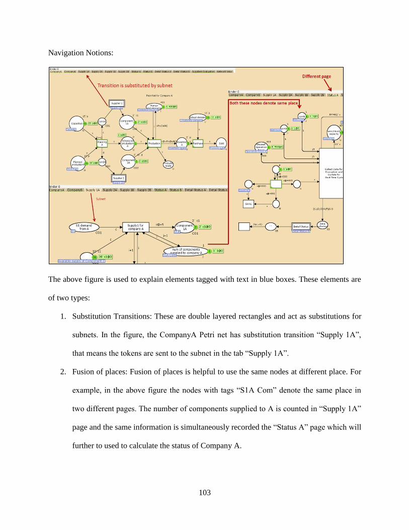
103
Navigation Notions:
The above figure is used to explain elements tagged with text in blue boxes. These elements are
of two types:
1. Substitution Transitions: These are double layered rectangles and act as substitutions for
subnets. In the figure, the CompanyA Petri net has substitution transition “Supply 1A”,
that means the tokens are sent to the subnet in the tab “Supply 1A”.
2. Fusion of places: Fusion of places is helpful to use the same nodes at different place. For
example, in the above figure the nodes with tags “S1A Com” denote the same place in
two different pages. The number of components supplied to A is counted in “Supply 1A”
page and the same information is simultaneously recorded the “Status A” page which will
further to used to calculate the status of Company A.

104
Petri net for events within Company A:
The user of the software could adjust the following in Petri net for Company A
Production Capacity: CapacityA is the production capacity of Company A. In the above net it
is set to 15 (1500 cars) for time period 300. This Capacity can be easily adjusted to desired value.
For this, the user has to click on 15`p and enter a new value in place of 15.
Other Initial values: Similarly the initial values of the places Component 1A, Component 2A,
Inventory A, Actual Demand and Human m/c resources can be adjusted to desired initial values.
Production time of a car: Outgoing arcs of transition “Production” contains the function
ProDelA() denoting the time taken to produce 100 cars (1token). In the ML code, ProDelA()=
PTA.ran() and colset PTA= int with 16..20, meaning that time to produce 100 cars is between 16
to 20 hours. The user can write its own function or change the values of 16 and 20. Similar
modifications can be done for any other functions specified in the ML code.
Similar Changes can be performed for Company B.

105
Petri net for transactions between Supplier 1 to Company A (similar to Supply 2A, 1B and 2B):
Petri net to collect data and update nodes at end of each time period for Company A:

106
Note: The data is collected in integer format with help of counter transitions. These are act as
accessory elements in the Petri net for counting of tokens and have no relation with supply chain
terminology.
Petri net (Detail Status A) to determine the status and the color zone of Company A (similar is
used for Company B):

107
Petri net to determine color zones of Supplier 1 and Supplier 2: