towards reliable modelling with stochastic process algebras
TRANSCRIPT
Towards Reliable Modelling with
Stochastic Process Algebras
Jeremy Thomas Bradley
Department of Computer Science
University of Bristol
October, 1999
A dissertation submitted to the University of Bristol in accordance with the
requirements for the degree of Doctor of Philosophy in the Faculty of Engineering.
Abstract
In this thesis, we investigate reliable modelling within a stochastic process
algebra framework. Primarily, we consider issues of variance in stochastic
process algebras as a measure of model reliability. This is in contrast to pre-
vious research in the �eld which has tended to centre around mean behaviour
and steady-state solutions.
We present a method of stochastic aggregation for analysing generally-distrib-
uted processes. This allows us more descriptive power in representing stochas-
tic systems and thus gives us the ability to create more accurate models.
We improve upon two well-developed Markovian process algebras and show
how their simpler paradigm can be brought to bear on more realistic syn-
chronisation models. Now, reliable performance �gures can be obtained for
systems, where previously only approximations of unknown accuracy were
possible.
Finally, we describe reliability de�nitions and variance metrics in stochastic
models and demonstrate how systems can be made more reliable through
careful combination under stochastic process algebra operators.
ii

Acknowledgements
My three years in the department in Bristol have been a lot of fun and the
person I have most to thank for this is my friend and mentor, Neil Davies.
I should also acknowledge the funding from NATS for my project and espe-
cially the help of Suresh Tewari (NATS) and Gordon Hughes (SSRC).
On the research side, I have to thank Judy Holyer, Peter Thompson, Ian
Holyer, Dave Tweed, Adel Jomah and Pauline Francis-Cobley, here in Bristol,
as well as Graham Clark, Stephen Gilmore, Jane Hillston, Nigel Thomas, Rob
Pooley and Helen Wilson whose comments, suggestions and encouragement
have all contributed enormously.
Personally, I would like to express my gratitude to Paul Dias, Chris Vowden,
Simon Sleight, Anders and Anne-Mette Spilling and my brother Tim, all of
whom saw both sides of the PhD and helped me survive.
To my parents, I owe a huge debt of thanks for supporting and encouraging
me tirelessly throughout my education, not to mention putting up with me
for the last three weeks of thesis-writing.
Finally, for Helen, who was always willing to listen, kept me going when it
all seemed fruitless and displayed incredible patience and strength from 7000
miles away|thank you for everything!
iii

To Helen
Declaration
I declare that the work in this dissertation was carried out in accordance
with the Regulations of the University of Bristol. The work is original except
where indicated by special reference in the text and no part of the dissertation
has been submitted for any other degree.
Any views expressed in the dissertation are those of the author and in no
way represent those of the University of Bristol.
The dissertation has not been presented to any other University for exami-
nation either in the United Kingdom or overseas.
Signed: Date:
v
Contents
Abstract ii
Acknowledgements iii
Declaration v
Contents vi
List of Figures xii
List of Tables xvii
1 Introduction 1
1.1 Modelling Communicating Systems . . . . . . . . . . . . . . . 1
1.2 Black-Box Modelling . . . . . . . . . . . . . . . . . . . . . . . 1
1.3 Fault-Tolerance and Timely Behaviour . . . . . . . . . . . . . 3
1.4 Our Research Goal . . . . . . . . . . . . . . . . . . . . . . . . 4
1.5 How this Document is Structured . . . . . . . . . . . . . . . . 4
vi
CONTENTS vii
1.6 Notation . . . . . . . . . . . . . . . . . . . . . . . . . . . . . . 5
2 Stochastic Process Algebras 7
2.1 Introduction . . . . . . . . . . . . . . . . . . . . . . . . . . . . 7
2.2 Process Algebras . . . . . . . . . . . . . . . . . . . . . . . . . 8
2.2.1 CCS|A Calculus of Communicating Systems . . . . . 9
2.3 Timed Process Algebras . . . . . . . . . . . . . . . . . . . . . 10
2.3.1 Temporal CCS . . . . . . . . . . . . . . . . . . . . . . 10
2.3.2 Timed CCS . . . . . . . . . . . . . . . . . . . . . . . . 11
2.4 Stochastic Process Algebras . . . . . . . . . . . . . . . . . . . 12
2.4.1 Introduction . . . . . . . . . . . . . . . . . . . . . . . . 12
2.4.2 Time and Action . . . . . . . . . . . . . . . . . . . . . 12
2.4.3 Markovian Process Algebras . . . . . . . . . . . . . . . 13
2.4.4 Generalised SPAs . . . . . . . . . . . . . . . . . . . . . 20
2.4.5 Generally-Distributed SPAs . . . . . . . . . . . . . . . 21
2.5 Other Stochastic Process Descriptions . . . . . . . . . . . . . . 22
2.5.1 Queueing Processes . . . . . . . . . . . . . . . . . . . . 22
2.5.2 Stochastic Extensions to Petri Nets . . . . . . . . . . . 23
2.6 Conclusion . . . . . . . . . . . . . . . . . . . . . . . . . . . . . 24
3 Analysing Stochastic Systems 26
3.1 Introduction . . . . . . . . . . . . . . . . . . . . . . . . . . . . 26
3.1.1 Stochastic Aggregation . . . . . . . . . . . . . . . . . . 27
3.2 Stochastic Transition Systems . . . . . . . . . . . . . . . . . . 29
CONTENTS viii
3.2.1 Introduction . . . . . . . . . . . . . . . . . . . . . . . . 29
3.2.2 Motivation . . . . . . . . . . . . . . . . . . . . . . . . . 30
3.2.3 De�nition . . . . . . . . . . . . . . . . . . . . . . . . . 31
3.2.4 Stochastic Aggregation . . . . . . . . . . . . . . . . . . 33
3.2.5 Equilibrium Distributions . . . . . . . . . . . . . . . . 35
3.2.6 Cox-Miller Normal Form . . . . . . . . . . . . . . . . . 36
3.2.7 Stochastic Normal Forms . . . . . . . . . . . . . . . . . 38
3.2.8 Worked Example . . . . . . . . . . . . . . . . . . . . . 44
3.3 Applications . . . . . . . . . . . . . . . . . . . . . . . . . . . . 48
3.3.1 Generally-Distributed Stochastic Process Algebras . . . 48
3.3.2 Queueing Systems . . . . . . . . . . . . . . . . . . . . 52
3.3.3 Markovian Process Algebras . . . . . . . . . . . . . . . 59
3.3.4 Component Analysis of a Stochastic Process Algebra
Model . . . . . . . . . . . . . . . . . . . . . . . . . . . 64
3.4 Conclusion . . . . . . . . . . . . . . . . . . . . . . . . . . . . . 68
3.A Probabilistic Operational Semantics of Stochastic Process Al-
gebras . . . . . . . . . . . . . . . . . . . . . . . . . . . . . . . 70
3.A.1 PEPA Operational Semantics . . . . . . . . . . . . . . 70
3.A.2 MTIPP Operational Semantics . . . . . . . . . . . . . 71
3.A.3 Operational Semantics of a GDSPA . . . . . . . . . . . 71
4 Synchronisation in SPAs 76
4.1 Introduction . . . . . . . . . . . . . . . . . . . . . . . . . . . . 76
4.2 Synchronisation in MPAs . . . . . . . . . . . . . . . . . . . . . 77
CONTENTS ix
4.3 Real-world Synchronisation Models . . . . . . . . . . . . . . . 78
4.3.1 Client-Server . . . . . . . . . . . . . . . . . . . . . . . 79
4.3.2 First-to-Finish . . . . . . . . . . . . . . . . . . . . . . . 79
4.3.3 Last-to-Finish . . . . . . . . . . . . . . . . . . . . . . . 81
4.3.4 N-to-Finish . . . . . . . . . . . . . . . . . . . . . . . . 83
4.3.5 Other Models . . . . . . . . . . . . . . . . . . . . . . . 84
4.4 Comparison with MPA Synchronisations . . . . . . . . . . . . 85
4.4.1 PEPA . . . . . . . . . . . . . . . . . . . . . . . . . . . 85
4.4.2 MTIPP . . . . . . . . . . . . . . . . . . . . . . . . . . 86
4.4.3 Comparing MTIPP and PEPA Synchronisations . . . . 88
4.5 Alternative Synchronisation Strategies . . . . . . . . . . . . . 90
4.5.1 Mean-preserving Synchronisation . . . . . . . . . . . . 90
4.5.2 Using PEPA to Bound the LTF Synchronisation . . . . 91
4.5.3 Restricted MTIPP Synchronisation . . . . . . . . . . . 92
4.6 A Worked Example . . . . . . . . . . . . . . . . . . . . . . . . 94
4.6.1 Markovian Model . . . . . . . . . . . . . . . . . . . . . 94
4.6.2 General Model . . . . . . . . . . . . . . . . . . . . . . 95
4.6.3 Comparative Solutions . . . . . . . . . . . . . . . . . . 96
4.6.4 Markovian Solution . . . . . . . . . . . . . . . . . . . . 97
4.6.5 Analytic Solution . . . . . . . . . . . . . . . . . . . . . 99
4.6.6 Model Comparisons . . . . . . . . . . . . . . . . . . . . 101
4.7 Conclusion . . . . . . . . . . . . . . . . . . . . . . . . . . . . . 106
4.7.1 Summary . . . . . . . . . . . . . . . . . . . . . . . . . 108
CONTENTS x
4.7.2 General Remarks . . . . . . . . . . . . . . . . . . . . . 112
4.A Comparative Stochastic Properties . . . . . . . . . . . . . . . 114
4.A.1 PEPA vs First-to-Finish . . . . . . . . . . . . . . . . . 114
4.A.2 MTIPP vs First-to-Finish . . . . . . . . . . . . . . . . 115
4.A.3 PEPA vs Last-to-Finish . . . . . . . . . . . . . . . . . 116
4.A.4 MTIPP vs Last-to-Finish . . . . . . . . . . . . . . . . . 116
4.A.5 MTIPP vs PEPA . . . . . . . . . . . . . . . . . . . . . 118
5 Reliability of Models in SPAs 119
5.1 Introduction . . . . . . . . . . . . . . . . . . . . . . . . . . . . 119
5.2 De�nitions of Reliability . . . . . . . . . . . . . . . . . . . . . 120
5.2.1 Real-Time Systems . . . . . . . . . . . . . . . . . . . . 121
5.2.2 Variance in Stochastic Transition Systems . . . . . . . 123
5.3 A General Stochastic Process Algebra . . . . . . . . . . . . . . 124
5.3.1 De�nition . . . . . . . . . . . . . . . . . . . . . . . . . 124
5.3.2 Variance Metric under SPA Combination . . . . . . . . 125
5.4 Speci�c Distributions under SPA Combination . . . . . . . . . 131
5.4.1 Competitive Choice and First-to-Finish Synchronisation133
5.4.2 Last-to-Finish Synchronisation . . . . . . . . . . . . . . 140
5.5 Worked Examples . . . . . . . . . . . . . . . . . . . . . . . . . 148
5.5.1 Search Algorithm . . . . . . . . . . . . . . . . . . . . . 148
5.5.2 Morse Code via Telephone . . . . . . . . . . . . . . . . 157
5.6 Conclusion . . . . . . . . . . . . . . . . . . . . . . . . . . . . . 163
5.6.1 Equivalences for Model Checking . . . . . . . . . . . . 163
CONTENTS xi
5.A General Variance Results . . . . . . . . . . . . . . . . . . . . . 166
5.A.1 Competitive Choice and First-to-Finish Synchronisation166
5.A.2 Last-to-Finish Synchronisation . . . . . . . . . . . . . . 168
5.B Minimum and Maximum Distributions of Random Variables . 169
5.B.1 Maximum Distribution . . . . . . . . . . . . . . . . . . 170
5.B.2 Minimum Distribution . . . . . . . . . . . . . . . . . . 170
6 Conclusions 172
6.1 Overview . . . . . . . . . . . . . . . . . . . . . . . . . . . . . . 172
6.2 Summary . . . . . . . . . . . . . . . . . . . . . . . . . . . . . 172
6.2.1 Introduction and Motivation . . . . . . . . . . . . . . . 172
6.2.2 Synchronisation . . . . . . . . . . . . . . . . . . . . . . 173
6.2.3 Reliability Modelling . . . . . . . . . . . . . . . . . . . 174
6.3 Speci�c Results . . . . . . . . . . . . . . . . . . . . . . . . . . 175
6.3.1 Stochastic Aggregation and Probabilistic Semantics . . 175
6.3.2 Synchronisation Classi�cation and Reliable Markovian
Modelling . . . . . . . . . . . . . . . . . . . . . . . . . 176
6.3.3 Classi�cation of Variance Reducing Operators and Dis-
tributions . . . . . . . . . . . . . . . . . . . . . . . . . 176
6.4 Further Investigation . . . . . . . . . . . . . . . . . . . . . . . 177
6.4.1 Component Aggregation . . . . . . . . . . . . . . . . . 177
6.4.2 Reliability through Feature Modelling . . . . . . . . . . 178
Bibliography 179
Index 190
List of Figures
2.1 A Petri net representation of the Dining Philosophers' problem. 24
3.1 A stochastic transition system with random variable transi-
tions and probabilistic branching. . . . . . . . . . . . . . . . . 29
3.2 The Cox-Miller Normal Form. . . . . . . . . . . . . . . . . . . 36
3.3 The set of normal forms for a state with �nite branching degree. 39
3.4 The digraph reduction rules. . . . . . . . . . . . . . . . . . . . 40
3.5 Rewriting the circuit c to have no vertices with multiple par-
ents except x. . . . . . . . . . . . . . . . . . . . . . . . . . . . 43
3.6 Rewriting the circuit c to have no vertices with multiple chil-
dren except x. . . . . . . . . . . . . . . . . . . . . . . . . . . . 43
3.7 A generally-distributed stochastic transition system. . . . . . . 45
3.8 Aggregating states 0 and 2 to give a Cox-Miller Normal Form
for state 1. . . . . . . . . . . . . . . . . . . . . . . . . . . . . . 45
3.9 Aggregating states 0 and 1 to give a Cox-Miller Normal Form
for state 2. . . . . . . . . . . . . . . . . . . . . . . . . . . . . . 46
3.10 Aggregating around state 0 to get a more complicated normal
form. . . . . . . . . . . . . . . . . . . . . . . . . . . . . . . . . 47
xii
LIST OF FIGURES xiii
3.11 Aggregating around state R, achieving a CMNF structure. . . 47
3.12 Aggregating around state S, achieving a CMNF structure. . . 47
3.13 The state diagram for a bu�er of a G/G/1/2 queue. . . . . . . 52
3.14 The stochastic transition system for a G/G/1/2 queue. . . . . 53
3.15 Aggregating the states 1 and 2 to produce a new state A and
an aggregated transition 1. . . . . . . . . . . . . . . . . . . . 55
3.16 Aggregating the states 0 and 1 to produce a new state B and
an aggregated transition 2. . . . . . . . . . . . . . . . . . . . 55
3.17 The process interleaving for a G/G/1/3 queue, taking into
account how many evolutions of the opposing process have
occurred. . . . . . . . . . . . . . . . . . . . . . . . . . . . . . . 58
3.18 A resource usage model in PEPA. . . . . . . . . . . . . . . . . 62
3.19 The state space of the resource usage model. . . . . . . . . . . 62
3.20 Using stochastic aggregation on a PEPA model with cooperation. 62
3.21 A simple PEPA example for component aggregation . . . . . . 65
3.22 Altering a component to re ect the stochastic e�ect of syn-
chronisations. . . . . . . . . . . . . . . . . . . . . . . . . . . . 65
3.23 The interleaved state space used to generate the Markov chain
in PEPA. . . . . . . . . . . . . . . . . . . . . . . . . . . . . . 67
3.24 Functional operational semantics for PEPA. . . . . . . . . . . 72
3.25 Probabilistic operational semantics for PEPA. . . . . . . . . . 73
3.26 Probabilistic operational semantics for MTIPP. . . . . . . . . 74
3.27 Probabilistic operational semantics for a generally-distributed
stochastic process algebra with pre-emptive restart. . . . . . . 75
LIST OF FIGURES xiv
4.1 The distribution of a First-to-Finish synchronisation of two
exponential transitions. . . . . . . . . . . . . . . . . . . . . . . 81
4.2 The distribution of a Last-to-Finish synchronisation of two
exponential transitions. . . . . . . . . . . . . . . . . . . . . . . 83
4.3 The distribution of a Last-to-Finish synchronisation and the
PEPA approximating cooperation. . . . . . . . . . . . . . . . . 86
4.4 The distribution of a Last-to-Finish synchronisation and the
MTIPP approximating synchronisation. . . . . . . . . . . . . . 88
4.5 The transition diagram for the Markovian process algebra sys-
tem of equations (4.37{4.41). The transition rate of the syn-
chronisation is expressed as �� to represent a generic MPA
synchronisation rate. . . . . . . . . . . . . . . . . . . . . . . . 95
4.6 Transition diagram for the generally distributed synchroni-
sation, X � exp( ) and Y � (A;B) where A � exp(�),
B � exp(�). p = IP(X < Y ). . . . . . . . . . . . . . . . . . . . 95
4.7 Time ratio: PEPA and PEPA* bound the analytic solution
with the mean-preserving model lying in between. . . . . . . . 105
4.8 Time ratio: all consistent MPAs overestimate the analytic so-
lution for these low value parameters, but the absolute error
is still small. . . . . . . . . . . . . . . . . . . . . . . . . . . . . 106
4.9 Time ratio: MTIPP can overestimate the analytic solution
considerably in some circumstances. . . . . . . . . . . . . . . . 107
4.10 Time ratio: if the parameter values are restricted to the ranges
in equation (4.32), then MTIPP can simulate LTF synchroni-
sation with reasonable accuracy. . . . . . . . . . . . . . . . . . 108
4.11 Number-of-transitions ratio: PEPA and PEPA* bound the an-
alytic solution with the mean-preserving model lying in between.109
LIST OF FIGURES xv
4.12 Number-of-transitions ratio: all consistent MPAs overestimate
the analytic solution for these low value parameters, but the
absolute error is still small. . . . . . . . . . . . . . . . . . . . . 110
4.13 Number-of-transitions ratio: MTIPP can overestimate the an-
alytic solution considerably in some circumstances. . . . . . . 111
4.14 Number-of-transitions ratio: if the parameter values are re-
stricted to the ranges in equation (4.32), then MTIPP can
simulate LTF synchronisation with reasonable accuracy. . . . . 112
5.1 The Laplacian path function de�nition, L1, for sequential and
choice combinators. . . . . . . . . . . . . . . . . . . . . . . . . 126
5.2 The Laplacian path function de�nition, L1, for synchronisa-
tion combinators. . . . . . . . . . . . . . . . . . . . . . . . . . 127
5.3 The variance reduction of a First-to-Finish synchronisation for
deterministic vs exponential. . . . . . . . . . . . . . . . . . . . 135
5.4 The variance reduction of a First-to-Finish synchronisation for
exponential vs exponential. . . . . . . . . . . . . . . . . . . . . 136
5.5 The variance reduction of a First-to-Finish synchronisation for
uniform vs deterministic. . . . . . . . . . . . . . . . . . . . . . 138
5.6 The variance reduction of a First-to-Finish synchronisation for
exponential vs uniform. . . . . . . . . . . . . . . . . . . . . . . 139
5.7 The variance reduction of a First-to-Finish synchronisation for
uniform vs exponential. . . . . . . . . . . . . . . . . . . . . . . 140
5.8 The variance reduction of a Last-to-Finish synchronisation for
deterministic vs exponential. . . . . . . . . . . . . . . . . . . . 142
5.9 The variance reduction of a Last-to-Finish synchronisation for
exponential vs exponential. . . . . . . . . . . . . . . . . . . . . 144
LIST OF FIGURES xvi
5.10 The variance reduction of a Last-to-Finish synchronisation for
uniform vs deterministic. . . . . . . . . . . . . . . . . . . . . . 146
5.11 The variance reduction of a Last-to-Finish synchronisation for
exponential vs uniform. . . . . . . . . . . . . . . . . . . . . . . 148
5.12 The variance reduction of a Last-to-Finish synchronisation for
uniform vs exponential. . . . . . . . . . . . . . . . . . . . . . . 149
5.13 Process algebra descriptions of the search algorithms. . . . . . 150
5.14 Stochastic transition system for random search algorithm. . . 150
5.15 �V1 against IE(T0) for �xed size array, N = 5: the introduc-
tion of the linear search produces a large variance reduction. . 152
5.16 �V2 against IE(T ) for �xed size array, N = 5: the introduction
of the random search produces a small variance reduction. . . 153
5.17 rV1 against IE(T0) for variable size array: relative to the orig-
inal random search, the linear search reduces the variance by
up to 93% for large N . . . . . . . . . . . . . . . . . . . . . . . 154
5.18 rV2 against IE(T ) for variable size array: relative to the origi-
nal linear search, the random search still reduces the variance
by up to 12% for large N . . . . . . . . . . . . . . . . . . . . . 155
5.19 rE1 against N : the mean reduces by up to 62% when the
linear search is combined with the random search, for large N . 156
5.20 rE2 against N : the mean reduces by 27% when the random
search is combined with the linear search, for large N . . . . . . 157
5.21 A process algebra description of Morse code over a ringing
phone. . . . . . . . . . . . . . . . . . . . . . . . . . . . . . . . 159
5.22 Stochastic transition system for the Morse code protocol. . . . 159
5.23 The bandwidth of dots and dashes in bits per minute, and the
equivalent probabilities of reception, for decreasing k. . . . . . 162
List of Tables
3.1 The stochastic equivalence of the two paths under reduction
rule R4. . . . . . . . . . . . . . . . . . . . . . . . . . . . . . . 41
3.2 The stochastic equivalence of the two paths under reduction
rule R5. . . . . . . . . . . . . . . . . . . . . . . . . . . . . . . 41
3.3 The distributions of successive transitions along the 2a, 1b cycle. 59
4.1 Some example values of tRESTART
and tSfor various Markovian
models. . . . . . . . . . . . . . . . . . . . . . . . . . . . . . . 104
4.2 Some example values of tRESUME
and tSfor various Markovian
models. . . . . . . . . . . . . . . . . . . . . . . . . . . . . . . 104
4.3 Some example values of nRESTART
and nSfor various Markovian
models. . . . . . . . . . . . . . . . . . . . . . . . . . . . . . . 105
xvii
Chapter 1
Introduction
1.1 Modelling Communicating Systems
Communicating systems are traditionally modelled using a black-box philos-
ophy that uses the mantra that observation is everything. This means that
a system is e�ectively de�ned by its outputs and its inputs and nothing else.
Any system which produces the same output in response to identical inputs
is considered an identical system. It may well be that the system achieves
its output using completely di�erent algorithms or hardware, but as long as
the external observable behaviour is preserved, that is all that matters. This
is encapsulated in the observational bisimilarity concept presented by Milner
in CCS [76, 77, 78].
1.2 Black-Box Modelling
This observationalist philosophy is not restricted to computer science or com-
puter systems|as might be expected, it has roots in experimental sciences
1
CHAPTER 1. INTRODUCTION 2
too. If a collection of atoms is excited and the resulting emitted light is
analysed spectrally, the various peaks in the wavelength spectrum betray the
constituent elements of the original atoms. In this case the input is the energy
that is expended on the atoms and the output constitutes the photons that
result. The implicit assumption is that the same entity is generating each
peak each time the experiment is performed. This con�dence is gained from
repeated experimentation on elements which also have behaved the same un-
der the same inputs. This is the key; all experimentation can be considered
to be an input to a system and the resulting behaviour, whether physical or
chemical, the output.
On a more grand scale, physicists' attempts to construct theories of the
universe fall into the same category. The models which they come up with
can only ever be at best observationally equivalent (bisimilar in CCS terms)
to reality. It can never be actually determined whether the correct internal
mechanisms have also been replicated. In the event that an experiment could
be devised which would betray a mechanism, then it would no longer be an
internal mechanism and would now constitute observable behaviour that any
correct theory or model would have to replicate or predict.
In arti�cial intelligence, observational bisimilarity is the basis for one of the
more famous thought experiments. Alan Turing proposed that if a system
could behave in a way indistinguishable from a human, then it would have
achieved intelligence. What makes this hard to verify in practice is that there
is no obvious formal de�nition of \indistinguishable" and similarly no formal
de�nition of what intelligent behaviour is or how much it can vary and still
be called intelligent.
This is where the formal de�nitions of bisimilarities of CCS and other calculi
come in to play. They allow relations to be de�ned which relate similarly be-
having systems, so in e�ect giving a rigorous meaning to the phrase \similarly
behaving".
CHAPTER 1. INTRODUCTION 3
1.3 Fault-Tolerance and Timely Behaviour
So how does this relate to the reliability requirements that an organisation
like the CAA1 requires of its systems and software?
There are two classes of reliability. There is the traditional functional cor-
rectness of a formally veri�ed system, where a logic tool such as Z or indeed
CCS is used to guarantee that correct operation will occur. Then there is
the timely behaviour of a system or temporal reliability, which reasons about
how long a system is likely to take to perform a task. It is the study of this
temporal reliability which is the subject of this project.
For the CAA both types of reliability are an issue. Both temporal and func-
tional reliability should make up their avour of observational bisimilarity.
Using such a avour, two systems might be identical if they both produce
the same outputs given the same inputs within a speci�c amount of time and
with a given probability.
A system may, with complete surety, �nd a minimum length solution to
the Travelling Salesman Problem, but if it takes many years to do so for a
required network, then this may only be of limited value. The point is that
the timing, or relative timing, of a result or output from a system (physical
or computational) is as much part of the observable behaviour as the actual
result itself.
This can be seen by going back to an example from the physical world. If a
system contains atoms of Carbon-14, then it is known that it is an element
of Carbon-14 because the half-life of the radioactive decay can be measured,
that is, the relative timings of the decays identify the element, not the type
of decay (in this case beta decay)|which is the same for many other isotopes
of other elements.
This extra timing expressiveness is absent from functional process algebras
such as CCS and adding it in has been the subject of a great deal of research
1The Civil Aviation Authority|NATS, a division of the CAA, sponsors this project.
CHAPTER 1. INTRODUCTION 4
in recent years. This thesis is particularly concerned with having the correct
type of timing model to allow us to talk about temporal reliability in as
general a way as possible.
To achieve this, we investigate timed stochastic extensions to CCS and the
like. These are known as stochastic process algebras and, in their most
general form, represent a completely general modelling environment for rep-
resenting real-world phenomena with either precision or uncertainty, as re-
quired.
1.4 Our Research Goal
Our research goal is �rst to investigate a su�ciently expressive modelling
paradigm, stochastic process algebras, that will allow us to express measures
of reliability. Reliability and performance inevitably go hand in hand, of-
ten involving a trade-o� of one for the other. Therefore, in this research,
we investigate both the accuracy of current performance modelling stochas-
tic process algebras, and methods for expressing and extracting reliability
measures from systems.
1.5 How this Document is Structured
Chapter 1 gives a high level perspective on some of the broader scienti�c and
philosophical issues which motivate this work.
Chapter 2 formally introduces some of the modelling techniques mentioned in
the introduction. It sets out general techniques for modelling communicating
systems and then gives an overview of other methodologies which make use
of timing and stochastic information. This chapter provides the necessary
background in which we set our work on reliability modelling in the rest of
the thesis.
CHAPTER 1. INTRODUCTION 5
Chapter 3 describes an analysis technique known as stochastic aggregation
that we use to compare some of the stochastic process algebra modelling tech-
niques from chapter 2. It provides interesting insights into some of the added
problems encountered when working with stochastically de�ned systems. We
go on to use this method continually in chapters 4 and 5.
Chapter 4 compares two Markovian process algebras, PEPA and MTIPP,
introduced in chapter 2, to measure their reliability in performance analysis.
It applies the stochastic aggregation techniques of chapter 3 to analyse the
accuracy of the two systems. This is one aspect of reliability|the ability
of a paradigm to reproduce accurately the correct results, or if making an
approximation to have an idea about how close the answer is to reality.
Chapter 5 speci�cally considers model reliability from a stochastic process
algebra perspective using the techniques of chapter 3. De�nitions and ways of
measuring reliability are suggested and some example systems are analysed.
In particular it is seen how the variance of a system plays a crucial role in
the reliability and predictability of a system.
Finally, chapter 6 summarises what we have covered and discusses how well
we have been able to achieve our reliability modelling goal. Future lines of
investigation are discussed.
1.6 Notation
Throughout this thesis, we use standard mathematical notation to represent
probabilistic concepts, in a style similar to that of Trivedi [97] and many
others. In particular:
Random variables are de�ned by X � exp(�), for instance, which means,
the random variable X samples from the exponential distribution with
parameter �. Other types of distribution used include: Gamma, �(n; �);
Uniform, U[a; b]; Deterministic, �(�); Hyperexponential, Hyper(�i;�i).
CHAPTER 1. INTRODUCTION 6
Distribution Functions are represented by f , F and L. The probability
distribution function of the random variable X would be fX(t); the cu-
mulative distribution function of X would be FX(t); and the Laplacian
of X would be LX(!). Occasionally we use FX(t) to mean the comple-
ment of the cumulative distribution function, so FX(t) = 1� FX(t).
Chapter 2
Stochastic Process Algebras
2.1 Introduction
In this chapter, we introduce traditional process algebras as a technique for
modelling communicating systems. We then discuss how process algebras
were augmented to include timing information. This serves as an introduction
to the main issue of the chapter: stochastic process algebras.
We will show why stochastic process algebras are more expressive than either
standard or timed process algebras. We will examine the current state of the
art in stochastic process algebras, concentrating on the analysis techniques
used. This is so that, in the �nal section, we can discuss the physical inter-
pretation of these analytical results and show why they are not su�cient on
their own to model reliability.
Having looked at system modelling from a process algebra perspective, we
will give a summary of two other stochastic techniques, stochastic Petri nets
and queueing networks. This completes our picture of stochastic modelling
since we then have a basis on which to compare stochastic process algebras
with other techniques.
7
CHAPTER 2. STOCHASTIC PROCESS ALGEBRAS 8
2.2 Process Algebras
Why use process algebras? There are many formalisms for representing com-
puter systems or communicating systems, so we need to justify selecting
process algebras. Milner [76] identi�es two key areas which he regarded as
central ideas behind his development of CCS: observation and synchronised
communication.
As discussed in chapter 1, modelling observable interaction is a very natural
way of de�ning the operation of an object, much more so because it lends itself
so easily to abstraction. Higher level modelling becomes simply a matter of
drawing larger black boxes around your components and hiding more internal
working.
The concept of synchronised communication that Milner talks about em-
bodies the whole mechanism of component-based modelling and concurrent
composition. Models can be succinctly de�ned in terms of simple components
which interact with each other to de�ne the operation of the whole.
This issue of parsimony (in this context, succinctness of expression) is also
important, both parsimony of the model and of the algebra. The �rst allows
for an easy conceptual construction and subsequent understanding of a model
while the second encourages further use of the paradigm. These are clearly
both essential qualities if a formalism is to be successful.
Then there are the reasons that any formalism is used at all|the very fact
that it provides a formal de�nition of a system means that ambiguities in
design have to be sorted out and errors removed. The understanding of a
system is always considerably improved by the use of a formal process and
this is bound to make for more reliable and consistent projects. Also as
a result of the formal expression process, a system can be formally and in
many cases automatically reasoned about. Properties such as livelock and
deadlock can be checked for; if a system invariant is speci�ed it can sometimes
be possible to verify formally the complete operation of the system against
that invariant (although this is usually restricted by practical computation
time and space limits).
CHAPTER 2. STOCHASTIC PROCESS ALGEBRAS 9
By no means least there is the �sthetic elegance of the language itself: the
fact that such a few language expressions can, when combined, de�ne a
complex communicating system|at least functionally. Examples of these
functional process algebras include CCS (Calculus of Communicating Sys-
tems) [76], CSP (Communicating Sequential Processes) [60, 61] and ACP
(Algebra for Communicating Processes) [7]; we use CCS below as an intro-
duction to the notation.
2.2.1 CCS|A Calculus of Communicating Systems
Milner de�nes CCS [76, 78] as follows:
P ::= 0 a:P P + P P jP PnL P [f ] A (2.1)
Pre�x a:P represents the evolution of either an input or output action where
a is an input event and a is an output. a:Pa�!P means a:P emits an
action a and proceeds to P .
Choice P + Q is a choice operator and means that if Pa�! P 0 then
P +Qa�! P 0 or if Q
b�! Q0 then P +Qb�! Q0.
Synchronisation P jQ denotes concurrent composition. If Pa�! P 0 and
Qa�! Q0 then P jQ ��! P 0jQ0 where � is a silent internal action. If the
actions do not form an input/output pair then the components evolve
una�ected by one another.
Restriction PnL. Speci�cally useful for abstraction and operation hiding:
actions in the set L are not observable outside the system P , i.e. they
do not evolve.
Relabelling P [f ] is a process P with its actions relabelled by a function f .
Useful for modularisation and component reuse.
Constant Adef= P is used to specify labels for parts (or agents) of a compo-
nent or system.
CHAPTER 2. STOCHASTIC PROCESS ALGEBRAS 10
In some extensions there is also an explicit recursion operator, �x(X = P ),
which behaves as P with occurrences of the variable X replaced by �x(X =
P ).
2.3 Timed Process Algebras
2.3.1 Temporal CCS
The development of Temporal CCS [95, 96] is an interesting one since it
encapsulates a subtle change in semantics to re ect a di�erent model of
timing.
In the �rst version of Temporal CCS [95], a system is presented as follows:
P ::= 0 X �[t]:P P + P P jP PnL P [S] �xXP (2.2)
where the pre�x �[t]:P represents a process which takes at least time t to
emit an action � and enter state P . The other combinators are similar to
traditional CCS.
A year later, the second version [96] had the following di�erences in de�nition:
P ::= 0 X �:P (t):P �:P P + P P jP : : : (2.3)
Here now, the timing aspect of the system is removed from the pre�x op-
eration. There is now an independent form (t):P which represents a delay
of exactly time t. The �:P describes a passive component which can wait
for an arbitrary amount of time before proceeding into state P . This is a
necessary addition for synchronising components, where one component gets
to a synchronising action �rst and has to wait for the other process to catch
up.
The major philosophical change was this devolution of action and time. This
was motivated by a result from quantum mechanics, as described in [96]:
CHAPTER 2. STOCHASTIC PROCESS ALGEBRAS 11
Computation involves energy change, and there is a result of
quantum mechanics which states that energy changes and time
cannot be measured simultaneously. Thus it seems reasonable
when producing an observation-based model of time and compu-
tation not to permit simultaneous observation of these two activ-
ities.
This obviously has implications for the type of timed process algebra we will
select for use in reliability modelling so we will discuss this issue later with
respect to stochastic process algebras (section 2.4.2).
A �nal form of Temporal CCS [79] used a similar system de�nition to that
of [96]:
P ::= 0 X �:P (t):P �:P P + P P jP : : : (2.4)
The pre�x operation is represented by �:P , the (t):P and �:P are as before
from [96]. The summation operator P + P is, for the �rst time, de�ned in
temporal context and called strong choice. A + B will behave as A if A
evolves �rst and B if B evolves before A.
2.3.2 Timed CCS
Whereas Temporal CCS expresses actions in terms of precise evolutions of
time, Timed CCS [21] models actions with intervals of time. This is an
important di�erence, since we can now deal with uncertainty in the modelling
process.
P ::= 0 X a(t)jpq:P P + P P jP PnL P [S] �xXP (2.5)
Here, the pre�x operation, written a(t)jpq:P , represents an action a which canoccur within an interval p < t < q after a has been initialised.
With the uncertainty in action execution, the model starts to describe almost
stochastic properties. This leads us nicely on to stochastic process algebras
which precisely represent this uncertainty, as we will see.
CHAPTER 2. STOCHASTIC PROCESS ALGEBRAS 12
2.4 Stochastic Process Algebras
2.4.1 Introduction
Stochastic process algebras di�er from standard process algebras or timed
process algebras by being able to represent spatial uncertainty explicitly|
which event happens next|and temporal uncertainty|when an event hap-
pens [50]. They do this by assigning a random variable amount of time to
the events of a system and having a method of probabilistic selection when
a choice of action is available.
Most stochastic process algebras sample the random variables for the action
times from exponential distributions with di�erent rates. These are called
Markovian process algebras and examples include PEPA [52], MTIPP [47],
EMPA [9] and MPA [20]. More recently there have been developments in
process algebras which allow for more generally-distributed action times; for
instance, originally, TIPP [37] and ET-LOTOS [2] then later, a Stochas-
tic Causality-Based Process Algebra [19], Stochastic �-Calculus [83] and
GSMPA [18].
2.4.2 Time and Action
In most stochastic process algebras, time and action have been recombined
in the pre�x operation. This might be seen as being contrary to the quantum
mechanical argument invoked by Tofts [96]|outlined in section 2.3.1.
The issue centres around whether time and action should be simultaneously
observable given that energy change and time are not, in a quantum me-
chanical system. The �rst thing to note is that this argument only applies at
the quantum level of interaction since Planck's constant is so small. Thus,
for all modelling tasks on a non-quantum scale, combining time and action
is a perfectly good approximation of reality. Indeed, the model itself is more
likely to be a far greater source of error. Also the combination of action and
CHAPTER 2. STOCHASTIC PROCESS ALGEBRAS 13
time is a natural abstraction to make from the modeller's point of view|a
calculation takes a particular amount of time.
If models do need to be constructed at a quantum scale, then how better
to express the uncertainty principle [28] than by using a stochastic process
algebra. If there is inherent uncertainty over the timing of an action, then
this can be represented using an appropriate probability density function.
For all these reasons most SPAs (stochastic process algebras) maintain a
direct link between action and timing1.
2.4.3 Markovian Process Algebras
A very good introduction to performance modelling with Markovian process
algebras is presented in Hermanns et al 1996 [44]. Markovian process algebras
can be generally represented using the syntax:
P ::= (a; �):P P + P P jjS P P=L A (2.6)
Pre�x (a; �):P is the pre�x operation and describes an action a taking a
random amount of time to occur. The random amount of time is sam-
pled from an exponential distribution of rate � and can therefore be in
the range 0 < t <1. This Markovian property also has the advantage
that, if after a time t0 the event has not occurred, then the remaining
conditional distribution is identical to the original exponential distri-
bution (see page 15 for details of the memoryless property).
Choice P + P represents a competitive choice between two processes. The
�rst process to evolve interrupts the other and the slower process is
discarded from the system. This is known as a race condition.
Synchronisation P jjS P is a synchronisation between two processes in-
volving only the actions in the set S. The exact nature of the synchro-
nisation di�ers from algebra to algebra, but it is usually intended that
1Hermanns' Interactive Markov Chains [43] is one of the few exceptions to this.
CHAPTER 2. STOCHASTIC PROCESS ALGEBRAS 14
the rate of the overall synchronised event will in some way re ect the
rate of the slower component.
A discussion of synchronisation strategies in the di�erent Markovian
process algebras can be found in Hillston 1994 [53]. One of the slightly
contentious issues surrounding Markovian process algebras is the fact
that the distribution describing the longer of two exponential distribu-
tions is itself not exponential. This means that technically MPAs do
not form a closed model2, however this is worked around in Marko-
vian process algebras by approximating the synchronisation event with
an exponential distribution. This issue and the consequences of the
approximation are the subject of chapter 4.
Hiding P=L hides the actions of P that occur in the set L. This is an
important modelling tool which allows internal events to be abstracted
away from other components. A hidden action becomes a � in the same
way as it does in CCS, however successive � 's can only be merged into
a single � (as in observational bisimulation in CCS) under conditions
of insensitivity (see section 3.1.1, which describes insensitivity).
Constant A := P is the constant agent. It allows labels to be assigned to
agents. By de�ning self-referential agents, recursion can be modelled.
The Performance Model
A performance model is obtained by establishing a translation from the al-
gebra to a continuous time Markov chain (CTMC). First the set of reachable
states Xi is constructed by eliminating component synchronisation using an
expansion law (discussed in the Markovian case below). The elements of the
in�nitesimal generator matrix (for further details of Markov chain solution,
2Stochastic process algebras which minimally incorporate immediate transitions as well
as exponential transitions such as EMPA [9, 8] and IMC [43, 45] can represent the maxi-
mum of two exponential distributions precisely.
CHAPTER 2. STOCHASTIC PROCESS ALGEBRAS 15
see for example [68, 63]) are assigned from the rates of the state transition
system:
Gij = r(Xi; Xj) : i 6= j (2.7)
where r(Xi; Xj) represents the total rate of transition from state Xi to Xj:
r(Xi; Xj) =Xk
XXi
(ak;�l)
���!Xj
�l (2.8)
Finally the diagonal elements are just:
Gii = �Xj
r(Xi; Xj) (2.9)
The steady-state probabilities � can be recovered from the equation:
�G = 0 (2.10)
subject toP
i �i = 1. These combined equations can be solved using Gaus-
sian elimination to obtain �. Now applying an appropriate reward structure
to the steady-state probabilities will theoretically extract the required quan-
titative performance �gures. A reward structure is just a weighting of the
states to re ect how important a particular state is for a particular property.
To construct a performance �gure p, we would use a reward structure rp:
p = rp � � =Xi
rpi�i (2.11)
The Memoryless Property
In stochastic terms, if X � exp(�) and t0 has elapsed then we are now
interested in the random variable Y = X � t0, given that X > t0, thus the
CHAPTER 2. STOCHASTIC PROCESS ALGEBRAS 16
distribution Y jX > t0:
FY jX>t0(t) = IP(Y � tjX > t0)
=IP(t0 < X � t+ t0)
IP(X > t0)
=1
FX(t0)
Z t+t0
t0fX(x) dx
= e�t0
(FX(t+ t0)� FX(t0))= e�t
0
(�e��(t+t0) + e��t0
)
= 1� e��t (2.12)
So Y jX > t0 � exp(�) as required. This is the memoryless property of the
exponential distribution and it is the only distribution to have this prop-
erty. It is important to the process algebra paradigm because it allows for a
relatively easy integration of stochastic processes into a CCS-like framework.
The expansion law of CCS rewrites a concurrent composition of components
in terms of a single component with a choice of evolution according to which
component evolves �rst.
C1j � � � jCn = a1:(C01j � � � jCn) + � � �+ an:(C1j � � � jC 0
n) (2.13)
for C1a1�! C 0
1; : : : ; Cnan�! C 0
n.
This rewriting is called an interleaving semantics and is only made possible
in Markovian process algebras because of the memoryless property of the
action durations.
If the memoryless property did not exist then a concurrent composition of
stochastic processes could not be rewritten in such a way. If one compo-
nent evolved before another enabled component then the description of the
residual distribution of the beaten component would have to take into ac-
count the distribution which beat it. This means that a memory of all the
evolved processes would have to be incorporated in any component which
was concurrently enabled.
CHAPTER 2. STOCHASTIC PROCESS ALGEBRAS 17
As it is, with exponential processes, a pre-empted process still behaves like
an exponential process and thus the same expansion law can be applied,
without any need to incorporate traces of previous evolution.
PEPA
PEPA (Performance Enhanced Process Algebra) was presented primarily
in [52, 55] and also [51, 50, 54]. PEPA has the following syntax:
P ::= (a; �):P P + P P ��SP P=L A (2.14)
The operators are identical to the description of a general Markovian pro-
cess algebra of section 2.4.3 except that the synchronisation operator is now
precisely de�ned. Cooperation, P ��SQ, is PEPA's method of specifying
component synchronisation. Operationally, if P(a;�)���! P 0, Q
(a;�)���! Q0 and
a 2 S then P ��SQ
(a;min(�;�))�������! P 0 ��SQ0, so the synchronised agent takes the
rate of the slower component.
The synchronisation is slightly complicated by the existence of many possible
a evolutions from the P and Q states. For this case, the apparent rate, ra(P ),
of a component is de�ned:
ra(P ) =X
P(a;�i)
���!
�i (2.15)
The reason for the name, apparent rate, is that when many identically la-
belled actions, a, are enabled simultaneously in a competitive choice, the
evolution is indistinguishable from a single action a being enabled with rate
ra(P ). However, if this situation occurs in a cooperation of components then
a particular a evolution has to be selected to participate in the cooperation.
So for any given evolution P(a;�i)���! the probability that it is the �rst one to
occur and thus participate in a cooperation is:
IP(Xi < min(Xj : j 6= i)) =�iPr �r
=�i
ra(P )(2.16)
CHAPTER 2. STOCHASTIC PROCESS ALGEBRAS 18
where Xr � exp(�r) and min(Xj : j 6= i) � exp(P
r 6=i �r).
So in the general case, if P(a;�)���!, Q
(a;�)���! and a 2 S then P ��SQ
(a;�)���!,
where:
� =�
ra(P )
�
ra(Q)min(ra(P ); ra(Q)) (2.17)
The term:
�
ra(P )
�
ra(Q)(2.18)
is a normalisation factor. The observable rate of the a-cooperation is in
fact just min(ra(P ); ra(Q)), however (for m a-evolutions from P and n a-
evolutions from Q) this is in turn made up of a choice between mn evolutions
where P �! Pi and Q �! Qj for speci�c i, j such that:
Xi;j
�ira(P )
�jra(Q)
min(ra(P ); ra(Q)) = min(ra(P ); ra(Q)) (2.19)
which is the overall apparent rate of the cooperation mentioned earlier.
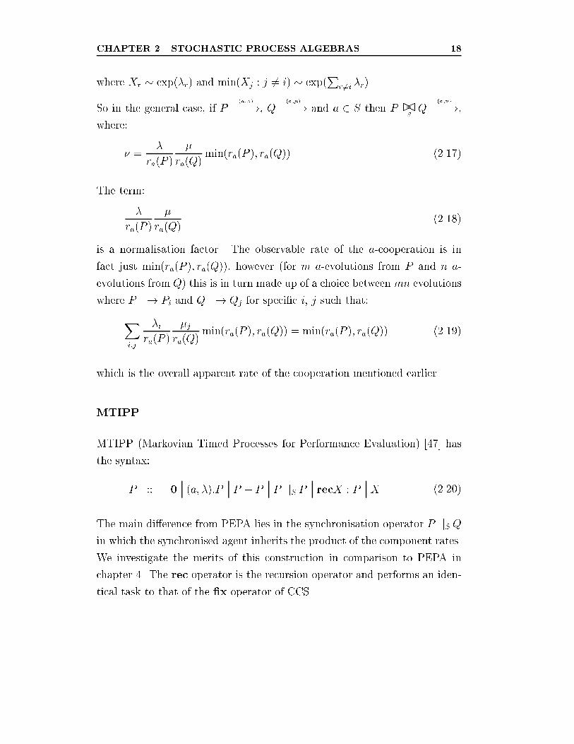
MTIPP
MTIPP (Markovian Timed Processes for Performance Evaluation) [47] has
the syntax:
P ::= 0 (a; �):P P + P P jjS P recX : P X (2.20)
The main di�erence from PEPA lies in the synchronisation operator P jjS Qin which the synchronised agent inherits the product of the component rates.
We investigate the merits of this construction in comparison to PEPA in
chapter 4. The rec operator is the recursion operator and performs an iden-
tical task to that of the �x operator of CCS.
CHAPTER 2. STOCHASTIC PROCESS ALGEBRAS 19
Markovian Process Algebras as a Modelling Paradigm
The trouble with Markovian process algebras is that it is di�cult either to
specify high level models accurately or to handle larger low level models
tractably.
In common with other formal modelling paradigms, initially it is useful to
be able to model at a high level of abstraction and rarely is it necessary to
model the very lowest level events. So, at a higher level, the atomic actions
will be a representation of a combination of more primitive actions (in some
aggregated form). These primitive actions may be exponential in character
but most combinations of them will not.
In summary, since the paradigm can only describe exponential and often
therefore low-level actions, it generates huge state-spaces and model descrip-
tions. These are, by de�nition, di�cult to handle both computationally and
conceptually. Further, it is not in general possible to abstract away from
the low-level description to make the model simpler or smaller, because the
modelling paradigm does not support the expressiveness to be able to do so.
So Markovian process algebras have their problems|we will see how other
stochastic process algebras overcome some of these problems in further sec-
tions. However, they are by far the easiest to solve for steady-state distribu-
tions via direct translation to a CTMC and tools exist to do just that [33, 46].
Also, there is considerable research being carried out in the use of approxima-
tion and simpli�cation techniques to reduce the model complexity problem
(product-form solutions [91, 58] through techniques such as stochastic re-
versibility [67, 59], quasi-reversibility [40] and quasi-separability [94, 93]).
Ultimately there may be considerable future in these product-form solutions
as bounding models which are considerably easier to manipulate than the
more complicated generally-distributed stochastic process algebras.
CHAPTER 2. STOCHASTIC PROCESS ALGEBRAS 20
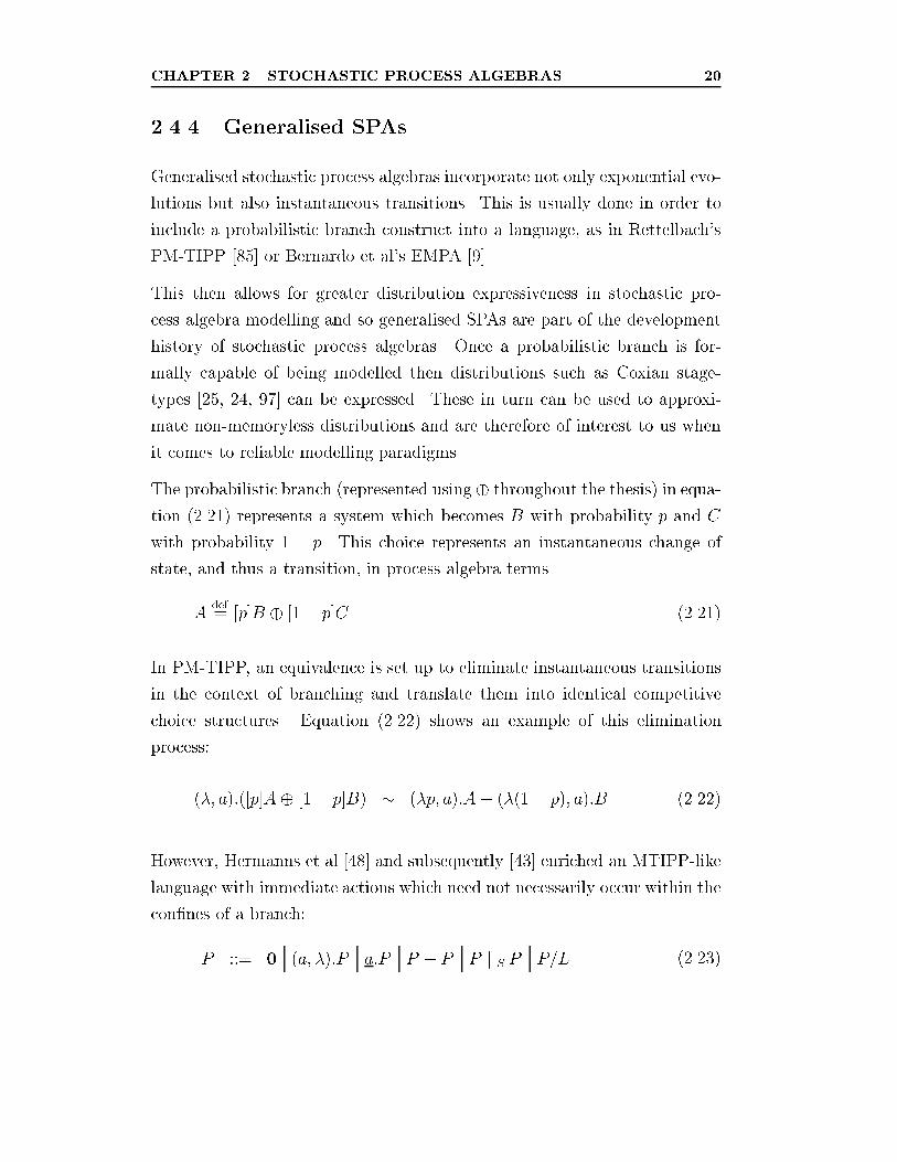
2.4.4 Generalised SPAs
Generalised stochastic process algebras incorporate not only exponential evo-
lutions but also instantaneous transitions. This is usually done in order to
include a probabilistic branch construct into a language, as in Rettelbach's
PM-TIPP [85] or Bernardo et al's EMPA [9].
This then allows for greater distribution expressiveness in stochastic pro-
cess algebra modelling and so generalised SPAs are part of the development
history of stochastic process algebras. Once a probabilistic branch is for-
mally capable of being modelled then distributions such as Coxian stage-
types [25, 24, 97] can be expressed. These in turn can be used to approxi-
mate non-memoryless distributions and are therefore of interest to us when
it comes to reliable modelling paradigms.
The probabilistic branch (represented using� throughout the thesis) in equa-
tion (2.21) represents a system which becomes B with probability p and C
with probability 1 � p. This choice represents an instantaneous change of
state, and thus a transition, in process algebra terms.
Adef= [p]B � [1� p]C (2.21)
In PM-TIPP, an equivalence is set up to eliminate instantaneous transitions
in the context of branching and translate them into identical competitive
choice structures. Equation (2.22) shows an example of this elimination
process:
(�; a):([p]A� [1� p]B) � (�p; a):A+ (�(1� p); a):B (2.22)
However, Hermanns et al [48] and subsequently [43] enriched an MTIPP-like
language with immediate actions which need not necessarily occur within the
con�nes of a branch:
P ::= 0 (a; �):P a:P P + P P jjS P P=L (2.23)
CHAPTER 2. STOCHASTIC PROCESS ALGEBRAS 21
where a:P represents the immediate occurrence of an a action. This then
has the advantage of allowing a precise representation of a slower-action or
Last-to-Finish (in the language of chapter 4) synchronisation.
It might be thought that immediate transitions might be easily approximated
by using exponential distributions with very high rates. This leads to sti�ness
problems when translated into the underlying Markov process. Numerical
solutions of such a system can become overrun by the much larger rate �gures
from the instantaneous transitions and the detail of the solution from the
slower, smaller rates can be lost.
In using such an algebra to model with Coxian stage-type distributions, how-
ever, we run the risk of generating huge underlying Markov chains for even
very simple models. A better solution still is to use a process algebra which
can work with general distributions directly.
2.4.5 Generally-Distributed SPAs
Generally-distributed stochastic process algebras are clearly of greatest inter-
est to us since they are far more expressive than Markovian process algebras
and are therefore more likely to be able to model a system accurately. An
accurate underlying stochastic model is going to be essential for meaningful
reliability analysis.
Although there are a few generally-distributed stochastic process algebras
that have de�ned the semantics necessary to deal with non-memoryless distri-
butions (TIPP [37], GSMPA [17, 18], Stochastic �-Calculus [83] and stochas-
tic bundle event structures [19]), few also provide a framework for generating
stochastic �gures, such as steady-state probabilities, and none consider issues
of reliability modelling.
In chapter 3, we will investigate a framework for describing and analysing
the generally-distributed stochastic processes in stochastic process algebras.
We will then apply this to judge the accuracy of Markovian process algebra
performance �gures in chapter 4 and then go on to develop reliability metrics
in chapter 5.
CHAPTER 2. STOCHASTIC PROCESS ALGEBRAS 22
2.5 Other Stochastic Process Descriptions
2.5.1 Queueing Processes
Queues are a set of stochastic processes, known as Birth-Death processes,
which have been analysed extensively [23, 70, 71, 5, 38] since Kendall's 1951
article outlining problems in the �eld [69].
Although they are considered too restrictive a model for general system mod-
elling, the wealth of stochastic results in the area will be useful to us when
trying to verify generally-distributed process algebra results in chapter 3.
A queue consists of an arrival process, a bu�er and one or more service
processes. A customer arrives according to some speci�ed distribution, is
queued in a (possibly in�nite) bu�er and is eventually serviced and removed
from the system.
Kendall laid down the foundations for describing a general queueing pro-
cess [69]. This has become known as Kendall notation. Using this form, a
queue is represented by the string: A/S/N[/K[/n]], where the last one or two
identi�ers may be omitted.
A describes the distribution of the arrival process. Some common values are
M for Markovian, GI or G for general independent, D for deterministic.
S describes the distribution of the service process.
N denotes the number of servers servicing the bu�er.
K represents the size of the bu�er. If omitted it is 1 by default.
n represents the number of customers. If omitted it is 1 by default.
If the bu�er is empty at any stage then the service process has to idle until
a customer arrives. Even then a full service time has to expire before that
customer is serviced. If the bu�er is full, then arriving customers may be
discarded or blocked.
CHAPTER 2. STOCHASTIC PROCESS ALGEBRAS 23
2.5.2 Stochastic Extensions to Petri Nets
Petri nets were �rst conceived by Carl Petri [81]. They predate traditional
process algebras at being able to model concurrent systems. However they
di�er from process algebras since they are speci�cally tailored to model pro-
cess causality rather than state transitions. They concentrate on resource and
process dependency and are largely orthogonal to process algebras, where the
emphasis is on composable inter-communicating components.
Petri nets are directed bipartite graphs. The nodes are split into two cate-
gories, places and transitions, with directed edges between the two categories.
Tokens ow through the graph, waiting in the places until all the places inci-
dent on a transition contain a token. At this stage the transition �res and at
least one of the tokens from each of the incident places moves to the places
immediately downstream of the �ring transition.
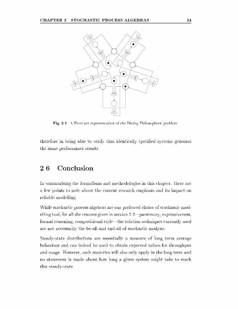
Each arrangement of tokens is called a marking and each marking is equiv-
alent to a state of a process. The collection of all reachable markings is
identical to the reachable states of a process. An example of a Petri net
is shown in �gure 2.1; the circles are the places and the rectangular bars
represent the transitions.
Stochastic �rings were �rst introduced into Petri nets by Molloy [80]. These
SPNs allowed transitions to �re with exponential delay and, similar to Marko-
vian process algebras, an underlying Markov chain model could be extracted
and solved for a steady-state distribution.
GSPNs (Generalised Stochastic Petri Nets) [4, 1] had both immediate and
exponential transitions present in the same net and still allowed the steady-
state probabilities to be derived. These were later extended to DSPNs (De-
terministic Stochastic Petri Nets) [3] which could incorporate Markovian and
deterministic transitions [74].
Although the disciplines of stochastic process algebras and stochastic Petri
nets are very di�erent in nature, they should still be capable of similar an-
alytical tasks. In a stochastic process algebra context SPNs are very useful
CHAPTER 2. STOCHASTIC PROCESS ALGEBRAS 24
Fig. 2.1. A Petri net representation of the Dining Philosophers' problem.
therefore in being able to verify that identically speci�ed systems generate
the same performance results.
2.6 Conclusion
In summarising the formalisms and methodologies in this chapter, there are
a few points to note about the current research emphasis and its impact on
reliable modelling.
While stochastic process algebras are our preferred choice of stochastic mod-
elling tool, for all the reasons given in section 2.2|parsimony, expressiveness,
formal reasoning, compositional style|the solution techniques currently used
are not necessarily the be-all and end-all of stochastic analysis.
Steady-state distributions are essentially a measure of long term average
behaviour and can indeed be used to obtain expected values for throughput
and usage. However, such statistics will also only apply in the long term and
no statement is made about how long a given system might take to reach
this steady-state.
CHAPTER 2. STOCHASTIC PROCESS ALGEBRAS 25
Ironically, as the Ehrenfest Paradox [67] indicates, a system in steady-state
equilibrium is also at its point of maximum entropy. This means that we
actually know least about it in this state, compared to when we started the
system o� or any other time in the systems history.
While long term statistics are de�nitely part of the picture when understand-
ing stochastic systems, there is a need to augment this information with some
idea of how much the system can vary while running. Measures of average
behaviour, by de�nition, remove any variant, extreme or tail-end behaviour.
This variation from the mean is exactly the type of behaviour that reliability
analysis is especially concerned with.
In chapter 5, we look at speci�cally this issue: how we can augment steady-
state information with concepts of extreme behaviour.
In the meantime, chapter 3 investigates steady-state solution techniques more
thoroughly and devises a method of stochastic analysis, called stochastic
aggregation, which we can apply to generally-distributed systems.
We are also interested in ensuring that accurate performance information
can be obtained from current tools. To this end, chapter 4 uses the stochas-
tic aggregation of chapter 3 to investigate the e�ects of the approximate
synchronisation models of Markovian process algebras, MTIPP and PEPA.
Chapter 3
Analysing Stochastic Systems
3.1 Introduction
In this chapter, we present a method of stochastic aggregation which e�ec-
tively reduces the structural complexity of a generally-distributed stochastic
system by embedding it into a probability distribution function within the
system. By reducing the structure to a simple normal form, we can tractably
undertake both performance and reliability analysis.
As discussed in chapter 2, if we are to have any success in modelling reliabil-
ity in systems, we need to be able to describe those systems accurately. Thus
we require the ability to model non-Markovian durations. Several process al-
gebras exist which semantically describe systems with generally-distributed
transitions [37, 2, 19, 83, 18]. However, the problem of analysing these sys-
tems in as general a way as possible is a mathematically hard one and many
of these systems cannot provide any solution techniques to produce, for in-
stance, performance statistics.
We introduce stochastic transitions systems as an underlying model for de-
26
CHAPTER 3. ANALYSING STOCHASTIC SYSTEMS 27
scribing an arbitrary stochastic process. We then consider how we might pro-
duce steady-state probabilities for this paradigm using a method of stochastic
aggregation (section 3.1.1, originally presented in [12]). By doing this, we
immediately give ourselves the ability to compare our results with steady-
state solutions from other paradigms, such as Markovian process algebras
and generally-distributed queues (sections 3.3.3 and 3.3.2). This gives us a
level of con�dence in our stochastic transitions system technique.
In the latter part of the chapter, we provide an alternative progressive solu-
tion method for Markovian process algebras which does not involve contin-
uous-time Markov chains. Also, with the aid of a queueing system, we demon-
strate why not having an interleaving semantics for generally-distributed con-
current processes becomes such a computational problem.
We show that we can obtain the complete steady-state distribution at the
component level of a generally-distributed stochastic process algebra (sec-
tion 3.2.7). There still remains the problem of how to analyse the synchro-
nising components that make up a fully-functioning system. To this end, we
round o� the chapter by demonstrating a component aggregation technique
(section 3.3.4): how it might be possible to analyse a generally-distributed
process algebra at a component level of the model. This would be similar
to a product form solution since it does not require the complete interleaved
state space generation that hampers other process algebras. Instead, com-
ponents can be analysed one at a time and the collective results from each
component would together form a steady-state distribution.
3.1.1 Stochastic Aggregation
Stochastic aggregation is a process of combining stochastic processes and
structures into a single process. It is a well-known result from Trivedi [97]
that program structures, such as if-then-else statements, while-loops and for-
loops, can be represented stochastically and then aggregated into a single
equivalent process. This allows us to aggregate sequences and combinations
of such structures into single processes.
CHAPTER 3. ANALYSING STOCHASTIC SYSTEMS 28
What we are able to do is show that for cyclic systems expressed in our
stochastic transition system, for each state, we can aggregate the system into
a normal form. These normal forms are special precisely because they can
be analytically solved to give stationary distributions. They also represent
a way of maintaining the complete stochastic nature of a system, but in a
reduced structural form.
The key to this aggregation technique is not to lose sight of the original
system totally. By carefully aggregating around a selected state, the normal
form is generated still containing a replica of that state, relative to the rest
of the system. Solving this normal form for the stationary distribution now
yields the correct stationary probability for the original state. This is then
repeated for the remaining states, to obtain the entire stationary distribution
for the whole system.
The method presented di�ers from a technique such as insensitivity anal-
ysis [75, 41, 87] in its general goal, since it speci�cally seeks not to change
the model under consideration. Insensitivity when applied to GSMPs (gener-
alised semi-Markov processes) [75] looks for structures of generally-distributed
processes which, when replaced with exponential processes with the same
mean, will still have the same steady-state distribution. Insensitivity has
been applied with signi�cant result to models of both generalised stochastic
Petri nets by Henderson [42] and stochastic process algebras by Clark [22].
However, given that ultimately we seek to obtain more than just steady-state
information (speci�cally in chapter 5), we require a framework which specif-
ically does not alter the model being analysed. By design, then, stochastic
aggregation preserves the stochastic nature of a system.
CHAPTER 3. ANALYSING STOCHASTIC SYSTEMS 29
3.2 Stochastic Transition Systems
3.2.1 Introduction
In this section, we present a solution technique for a generally-distributed
stochastic transition system. The method was inspired by an example origi-
nally presented in Cox and Miller [26]; it has been extended to use general-
distributions and, through aggregation, provides a solution technique for
more than the original two state system.
A transition system is de�ned to describe individual evolutions from state
to state. Time is represented along each transition by a continuous random
variable and it is these random variables which can take any distribution
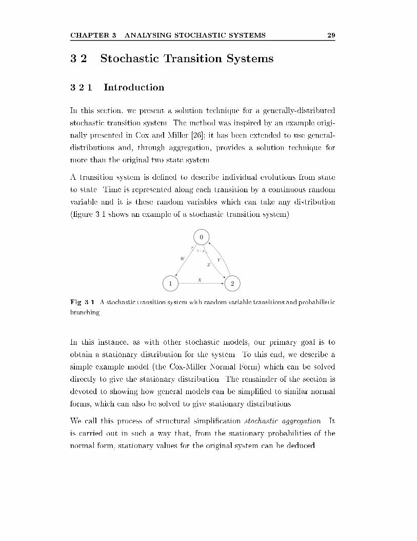
(�gure 3.1 shows an example of a stochastic transition system).
Fig. 3.1. A stochastic transition system with random variable transitions and probabilistic
branching.
In this instance, as with other stochastic models, our primary goal is to
obtain a stationary distribution for the system. To this end, we describe a
simple example model (the Cox-Miller Normal Form) which can be solved
directly to give the stationary distribution. The remainder of the section is
devoted to showing how general models can be simpli�ed to similar normal
forms, which can also be solved to give stationary distributions.
We call this process of structural simpli�cation stochastic aggregation. It
is carried out in such a way that, from the stationary probabilities of the
normal form, stationary values for the original system can be deduced.
CHAPTER 3. ANALYSING STOCHASTIC SYSTEMS 30
3.2.2 Motivation
In designing a stochastic transition system, we are keen to avoid many of
the complexities that make other generally-distributed systems (queueing
systems, for instance) very di�cult to solve. In particular, by steering clear
of any notion of concurrent evolution, it is seen that the memoryless issue
can be avoided at this stage. Although it is clear that we are reducing the
expressiveness of our language by doing so, a solution technique for some
class of generally-distributed system is still of interest to us. We will see
later that we are still able to model even generally-distributed concurrent
processes with careful mapping.
While studying some results and methods from single-server �nite queues,
the question kept on arising: `What is the actual distribution between this
state and the next one?'. It became apparent that saying that a queue had
a generally-distributed service time was attributing a high level description
to the queue, much as a process algebra might do. Precisely as a result of
complexities like memory, the actual inter-state distributions were distinct,
complex and certainly not obvious from the stated general distribution (see
discussion on queueing systems in section 3.3.2, especially).
From section 2.4.3, we know that Markovian queues or systems do not have
to cope with this complication of distribution memory since they are memo-
ryless. In saying that a queue is Markovian, the transitions of its stochastic
transition system are immediately attributed exponential distributions. It
turns out there are many such simpli�cations and �nesses that can be per-
formed by using Markovian processes, which, of course, is why they are so
useful and so heavily studied. However they do have the drawback of hid-
ing a lot of the underlying stochastic complexity; complexity which has a
direct bearing on reliable modelling, when we analyse generally-distributed
systems.
From observing that some kind of underlying state transition system was
behind the operation of such generally-distributed systems, it is a natural step
CHAPTER 3. ANALYSING STOCHASTIC SYSTEMS 31
to want to describe and solve such a model. In this way the use of techniques
such as embedded Markov chains might be avoided. This is desirable because,
though a clever application, the embedded Markov chain in queues is very
reliant on the simple Birth-Death structure of the queue. Such nice structural
properties cannot be assumed for general process graphs, which are typically
described by process algebras.
With this in mind, it seemed necessary to abstract concepts like action labels,
competitive choice and parallel composition up to a process algebra level.
It will be seen in later sections how such higher level functionality can be
reintroduced.
3.2.3 De�nition
We de�ne a stochastic transition system to be a directed labelled graph.
For the purposes of stationary distribution analysis let the digraph be bi-
connected, by which we mean that any vertex (state) is reachable from any
other vertex, via a directed path. This latter condition is the equivalent of
the structural ergodic condition for PEPA [52] and ensures that a stationary
distribution exists.
In operation, a process will start in a designated state and proceed to follow
one and only one path round the graph. At no stage, therefore, does memory
become an issue since the process is only executing one transition at a time,
in sequence.
In algebraic terms we de�ne a state, S to be:
S ::= fXg:S [p]S � [1� p]S A (3.1)
where X represents a continuous positive random variable and p, 0 < p < 1
is a probability and A is a constant label.
The �rst operator is analogous to the pre�x operator in CCS [78] and repre-
sents a sequential process, which pauses for a duration X before proceeding
to the next transition.
CHAPTER 3. ANALYSING STOCHASTIC SYSTEMS 32
The second operator, �, represents branching. As can be seen from the
de�nition, we have adopted probabilistic branching, mainly for reasons of
simplicity given above. The selection of a path is instantaneous and samples
from a Bernoulli trial (parameter, p) to decide which branch to take.
For the algebraic model to match the graph description, it remains to be
demonstrated how n-way branching in the digraph is treated. For this, we
simply need a structural associativity law to enable us to treat the n-way
branch in a pairwise fashion.
Let:
Sdef= [p]T � [1� p]fZg:S3 (3.2)
Tdef= [q]fXg:S1 � [1� q]fY g:S2 (3.3)
We require that:
Sdef= [m]fXg:S1 � [1�m]U (3.4)
Udef= [n1]fY g:S2 � [n2]fZg:S3 (3.5)
such that n1 + n2 = 1.
Now:
IP(S1 is reached from S) = pq (3.6)
IP(S2 is reached from S) = p(1� q) (3.7)
IP(S3 is reached from S) = 1� p (3.8)
given that the branch probabilities are independent Bernoulli trials. Now we
can see that, for the second model to be consistent with the �rst:
CHAPTER 3. ANALYSING STOCHASTIC SYSTEMS 33
1. For state S1:
m = pq (3.9)
2. For states S2, S3:
n1(1� pq) = p(1� q) (3.10)
n2(1� pq) = 1� p (3.11)
Now:
n1 + n2 =p� pq1� pq +
1� p1� pq = 1 (3.12)
as required.
From this result, a general n-way probabilistic branch,Ln
i=1[pi]Si wherePni=1 pi = 1, can be de�ned recursively, for n � 2:
nMi=1
[pi]Sidef= [pn � 1]
n�1Mi=1
�pi
pn � 1
�Si
!� [pn]Sn (3.13)
2Mi=1
[pi]Sidef= [p1]S1 � [p2]S2 (3.14)
3.2.4 Stochastic Aggregation
Here, we describe a technique called stochastic aggregation, which forms
the basis of our solution technique for stochastic transition systems. The
rules presented come from Trivedi 1982 [97] where they described program
execution; they have been rewritten below to describe a stochastic transition
system.
The associativity of probabilistic branching (section 3.2.3) means that it is
su�cient to consider two-way branching in equations (3.17) and (3.19).
CHAPTER 3. ANALYSING STOCHASTIC SYSTEMS 34
Stochastic aggregation was born out of a need to try and reduce system
complexity by combining (or aggregating) the edges and states of the tran-
sition graph. In doing so, it replaces a structure of the graph with a smaller
equivalent structure, which takes the same amount of time to execute as the
original.
Throughout, stochastic aggregation is de�ned in terms of Laplace transforms.
Convolution
Two sequential processes are aggregated into one:
Adef= fX1g:fX2g:B ���! A
def= fY g:B (3.15)
From the standard convolution result of Laplace transforms [98], we get:
LY (!) = LX1+X2(!) = LX1(!)LX2(!) (3.16)
Branching
A branch point where both branches eventually recombine, can be aggregated
into a single process:
Adef= [p]fX1g:B � [1� p]fX2g:B ���! A
def= fY g:B (3.17)
where:
LY (!) = pLX1(!) + (1� p)LX2(!) (3.18)
Terminating Loop
A process that loops with probability (1 � p), or takes an alternative path
with probability p, can be aggregated into a single process:
CHAPTER 3. ANALYSING STOCHASTIC SYSTEMS 35
Adef= [p]fX1g:B � [1� p]fX2g:A ���! A
def= fY g:B (3.19)
It can be derived from [97] that:
LY (!) =pLX1(!)
1� (1� p)LX2(!)(3.20)
3.2.5 Equilibrium Distributions
Before we launch into our �rst instance of solving a system for its equilibrium
distribution, we must �rst discuss some properties of equilibrium distribu-
tions themselves. These are taken from Cox and Miller 1965 [26].
Given a state transition system:
1. For all initial conditions the probability pi(t) that state i is occupied
at time t tends to a distribution f�j : 1 � j � ng as t �!1.
2. If the initial state has the probability distribution f�j : 1 � j � ngthen pi(t) = �i for all t.
3. After a long time t0, the proportion of time spent in any state i con-
verges to �i as t0 �!1.
4. The equilibrium probabilities, �i, if they exist, satisfy a system of or-
dinary simultaneous linear equations.
These properties lead to the following empirical interpretations of stationary
distributions:
1. Given a large number of independent realisations (traces) of a system:
at a large time t0, the proportion of systems in state i tends to �i.
2. Given a single long realisation, the proportion of time spent in state i
tends to �i.
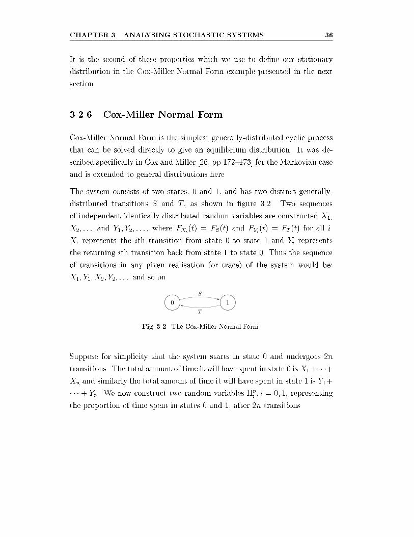
CHAPTER 3. ANALYSING STOCHASTIC SYSTEMS 36
It is the second of these properties which we use to de�ne our stationary
distribution in the Cox-Miller Normal Form example presented in the next
section.
3.2.6 Cox-Miller Normal Form
Cox-Miller Normal Form is the simplest generally-distributed cyclic process
that can be solved directly to give an equilibrium distribution. It was de-
scribed speci�cally in Cox and Miller [26, pp.172{173] for the Markovian case
and is extended to general distributions here.
The system consists of two states, 0 and 1, and has two distinct generally-
distributed transitions S and T , as shown in �gure 3.2. Two sequences
of independent identically distributed random variables are constructed X1,
X2; : : : and Y1; Y2; : : : , where FXi(t) = FS(t) and FYi(t) = FT (t) for all i.
Xi represents the ith transition from state 0 to state 1 and Yi represents
the returning ith transition back from state 1 to state 0. Thus the sequence
of transitions in any given realisation (or trace) of the system would be:
X1; Y1; X2; Y2; : : : and so on.
Fig. 3.2. The Cox-Miller Normal Form.
Suppose for simplicity that the system starts in state 0 and undergoes 2n
transitions. The total amount of time it will have spent in state 0 isX1+� � �+Xn and similarly the total amount of time it will have spent in state 1 is Y1+
� � �+ Yn. We now construct two random variables �ni ; i = 0; 1, representing
the proportion of time spent in states 0 and 1, after 2n transitions.
CHAPTER 3. ANALYSING STOCHASTIC SYSTEMS 37
�n0 =
X1 + � � �+Xn
X1 + Y1 +X2 + Y2 + � � �+Xn + Yn
=1n
Pni=1Xi
1n
Pni=1Xi +
1n
Pni=1 Yi
=X
X + Y(3.21)
Similarly:
�n1 =
Y
X + Y(3.22)
where X and Y are sample means of the n independent random variables.
We now utilise the Strong Law of Large Numbers [30, p.243] to relate the
sample means of Xi and Yi to the distribution means of S and T .
Thm. 1 (The Strong Law of Large Numbers). Let Xk be a sequence
of mutually independent random variables with a common distribution. If
the expectation � = IE(Xk) exists, then for every " > 0 as n �!1:
IP
�����X1 + � � �+Xn
n� �
���� < "
��! 1 (3.23)
Now applying this to our sample means X and Y , for all " > 0:
limn�!1
IP(jX � IE(S)j < ") = 1
) IP�limn�!1
X = IE(S)�= 1 (3.24)
Similarly:
IP�lim
n�!1Y = IE(T )
�= 1 (3.25)
So when the limit is applied to �ni , we get:
IP
�lim
n�!1�n0 =
IE(S)
IE(S) + IE(T )
�= 1 (3.26)
CHAPTER 3. ANALYSING STOCHASTIC SYSTEMS 38
IP
�lim
n�!1�n1 =
IE(T )
IE(S) + IE(T )
�= 1 (3.27)
From our de�nition of an equilibrium distribution:
limn�!1
�ni = �i (3.28)
So we can now obtain �0 and �1:
�0 =IE(S)
IE(S) + IE(T )(3.29)
�1 =IE(T )
IE(S) + IE(T )(3.30)
With hindsight, we can see that since the steady-state distribution of Cox-
Miller Normal Form is a function solely of the means of the constituent
distributions, then it is insensitive to the type of the general distributions,
S and T . This means that we could also have obtained the solution by
substituting the general distributions with exponential distributions of the
same mean and solving the resulting Markovian process to get the same
answer as presented in equations (3.29) and (3.30).
While the steady-state distribution is certainly a useful comparative metric,
this insensitivity is a good demonstration of quite how much distribution
information is lost in the �nal result. The steady-state is very much a mea-
sure of average behaviour and this bears out our summary of it, given in
section 2.6.
3.2.7 Stochastic Normal Forms
Motivation
In this section, we show that general systems can be reduced to a normal
form, using stochastic aggregation. The simplest of these normal forms is
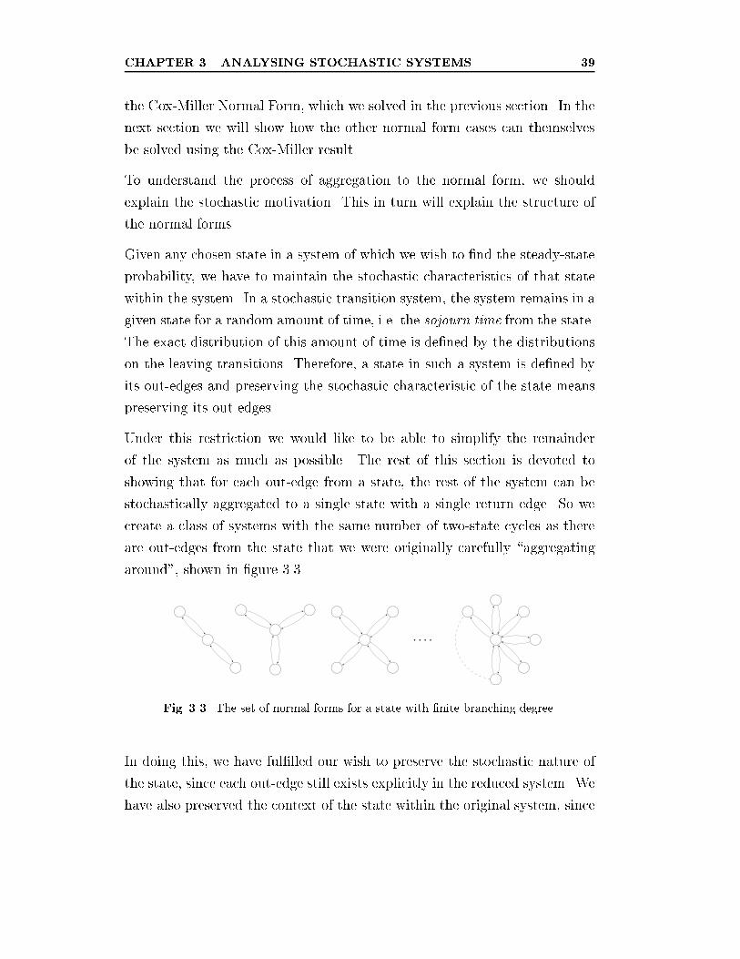
CHAPTER 3. ANALYSING STOCHASTIC SYSTEMS 39
the Cox-Miller Normal Form, which we solved in the previous section. In the
next section we will show how the other normal form cases can themselves
be solved using the Cox-Miller result.
To understand the process of aggregation to the normal form, we should
explain the stochastic motivation. This in turn will explain the structure of
the normal forms.
Given any chosen state in a system of which we wish to �nd the steady-state
probability, we have to maintain the stochastic characteristics of that state
within the system. In a stochastic transition system, the system remains in a
given state for a random amount of time, i.e. the sojourn time from the state.
The exact distribution of this amount of time is de�ned by the distributions
on the leaving transitions. Therefore, a state in such a system is de�ned by
its out-edges and preserving the stochastic characteristic of the state means
preserving its out-edges.
Under this restriction we would like to be able to simplify the remainder
of the system as much as possible. The rest of this section is devoted to
showing that for each out-edge from a state, the rest of the system can be
stochastically aggregated to a single state with a single return edge. So we
create a class of systems with the same number of two-state cycles as there
are out-edges from the state that we were originally carefully \aggregating
around", shown in �gure 3.3.
Fig. 3.3. The set of normal forms for a state with �nite branching degree.
In doing this, we have ful�lled our wish to preserve the stochastic nature of
the state, since each out-edge still exists explicitly in the reduced system. We
have also preserved the context of the state within the original system, since
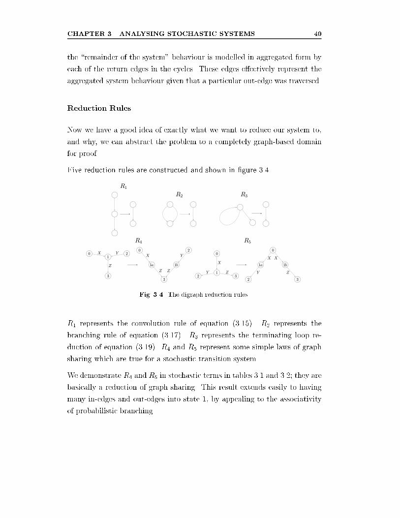
CHAPTER 3. ANALYSING STOCHASTIC SYSTEMS 40
the \remainder of the system" behaviour is modelled in aggregated form by
each of the return edges in the cycles. These edges e�ectively represent the
aggregated system behaviour given that a particular out-edge was traversed.
Reduction Rules
Now we have a good idea of exactly what we want to reduce our system to,
and why, we can abstract the problem to a completely graph-based domain
for proof.
Five reduction rules are constructed and shown in �gure 3.4.
Fig. 3.4. The digraph reduction rules.
R1 represents the convolution rule of equation (3.15). R2 represents the
branching rule of equation (3.17). R3 represents the terminating loop re-
duction of equation (3.19). R4 and R5 represent some simple laws of graph
sharing which are true for a stochastic transition system.
We demonstrate R4 and R5 in stochastic terms in tables 3.1 and 3.2; they are
basically a reduction of graph sharing. This result extends easily to having
many in-edges and out-edges into state 1, by appealing to the associativity
of probabilistic branching.
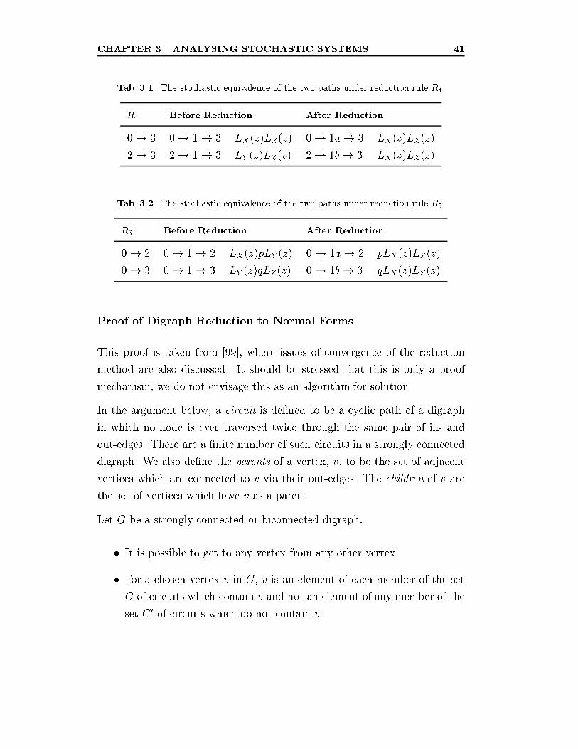
CHAPTER 3. ANALYSING STOCHASTIC SYSTEMS 41
Tab. 3.1. The stochastic equivalence of the two paths under reduction rule R4.
R4 Before Reduction After Reduction
0! 3 0! 1! 3 LX(z)LZ(z) 0! 1a! 3 LX(z)LZ(z)
2! 3 2! 1! 3 LY (z)LZ(z) 2! 1b! 3 LX(z)LZ(z)
Tab. 3.2. The stochastic equivalence of the two paths under reduction rule R5.
R5 Before Reduction After Reduction
0! 2 0! 1! 2 LX(z)pLY (z) 0! 1a! 2 pLX(z)LZ(z)
0! 3 0! 1! 3 LY (z)qLZ(z) 0! 1b! 3 qLX(z)LZ(z)
Proof of Digraph Reduction to Normal Forms
This proof is taken from [99], where issues of convergence of the reduction
method are also discussed. It should be stressed that this is only a proof
mechanism, we do not envisage this as an algorithm for solution.
In the argument below, a circuit is de�ned to be a cyclic path of a digraph
in which no node is ever traversed twice through the same pair of in- and
out-edges. There are a �nite number of such circuits in a strongly connected
digraph. We also de�ne the parents of a vertex, v, to be the set of adjacent
vertices which are connected to v via their out-edges. The children of v are
the set of vertices which have v as a parent.
Let G be a strongly connected or biconnected digraph:
� It is possible to get to any vertex from any other vertex.
� For a chosen vertex v in G, v is an element of each member of the set
C of circuits which contain v and not an element of any member of the
set C 0 of circuits which do not contain v.
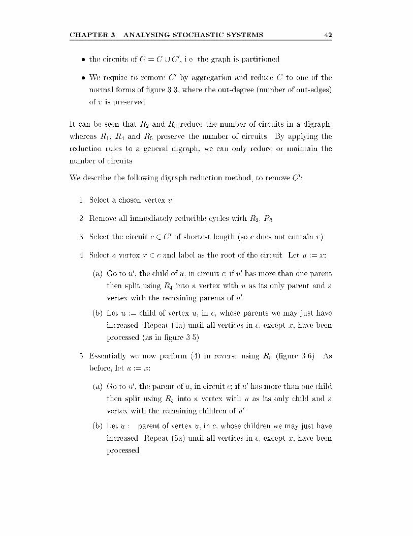
CHAPTER 3. ANALYSING STOCHASTIC SYSTEMS 42
� the circuits of G = C [ C 0, i.e. the graph is partitioned.
� We require to remove C 0 by aggregation and reduce C to one of the
normal forms of �gure 3.3, where the out-degree (number of out-edges)
of v is preserved.
It can be seen that R2 and R3 reduce the number of circuits in a digraph,
whereas R1, R4 and R5 preserve the number of circuits. By applying the
reduction rules to a general digraph, we can only reduce or maintain the
number of circuits.
We describe the following digraph reduction method, to remove C 0:
1. Select a chosen vertex v.
2. Remove all immediately reducible cycles with R2, R3.
3. Select the circuit c 2 C 0 of shortest length (so c does not contain v).
4. Select a vertex x 2 c and label as the root of the circuit. Let u := x:
(a) Go to u0, the child of u, in circuit c; if u0 has more than one parent
then split using R4 into a vertex with u as its only parent and a
vertex with the remaining parents of u0.
(b) Let u := child of vertex u, in c, whose parents we may just have
increased. Repeat (4a) until all vertices in c, except x, have been
processed (as in �gure 3.5).
5. Essentially we now perform (4) in reverse using R5 (�gure 3.6). As
before, let u := x:
(a) Go to u0, the parent of u, in circuit c; if u0 has more than one child
then split using R5 into a vertex with u as its only child and a
vertex with the remaining children of u0.
(b) Let u := parent of vertex u, in c, whose children we may just have
increased. Repeat (5a) until all vertices in c, except x, have been
processed.
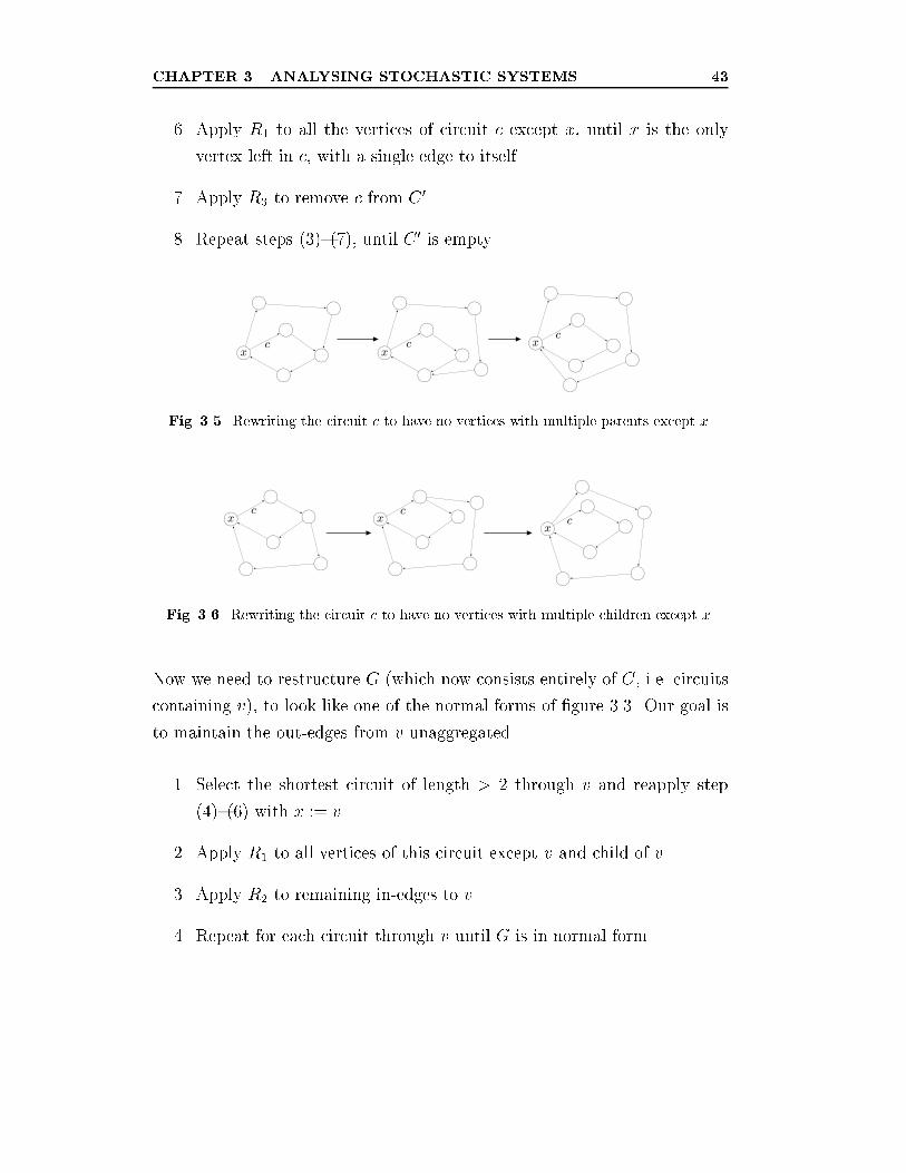
CHAPTER 3. ANALYSING STOCHASTIC SYSTEMS 43
6. Apply R1 to all the vertices of circuit c except x, until x is the only
vertex left in c, with a single edge to itself.
7. Apply R3 to remove c from C 0.
8. Repeat steps (3){(7), until C 0 is empty.
Fig. 3.5. Rewriting the circuit c to have no vertices with multiple parents except x.
Fig. 3.6. Rewriting the circuit c to have no vertices with multiple children except x.
Now we need to restructure G (which now consists entirely of C, i.e. circuits
containing v), to look like one of the normal forms of �gure 3.3. Our goal is
to maintain the out-edges from v unaggregated.
1. Select the shortest circuit of length > 2 through v and reapply step
(4){(6) with x := v.
2. Apply R1 to all vertices of this circuit except v and child of v.
3. Apply R2 to remaining in-edges to v.
4. Repeat for each circuit through v until G is in normal form.
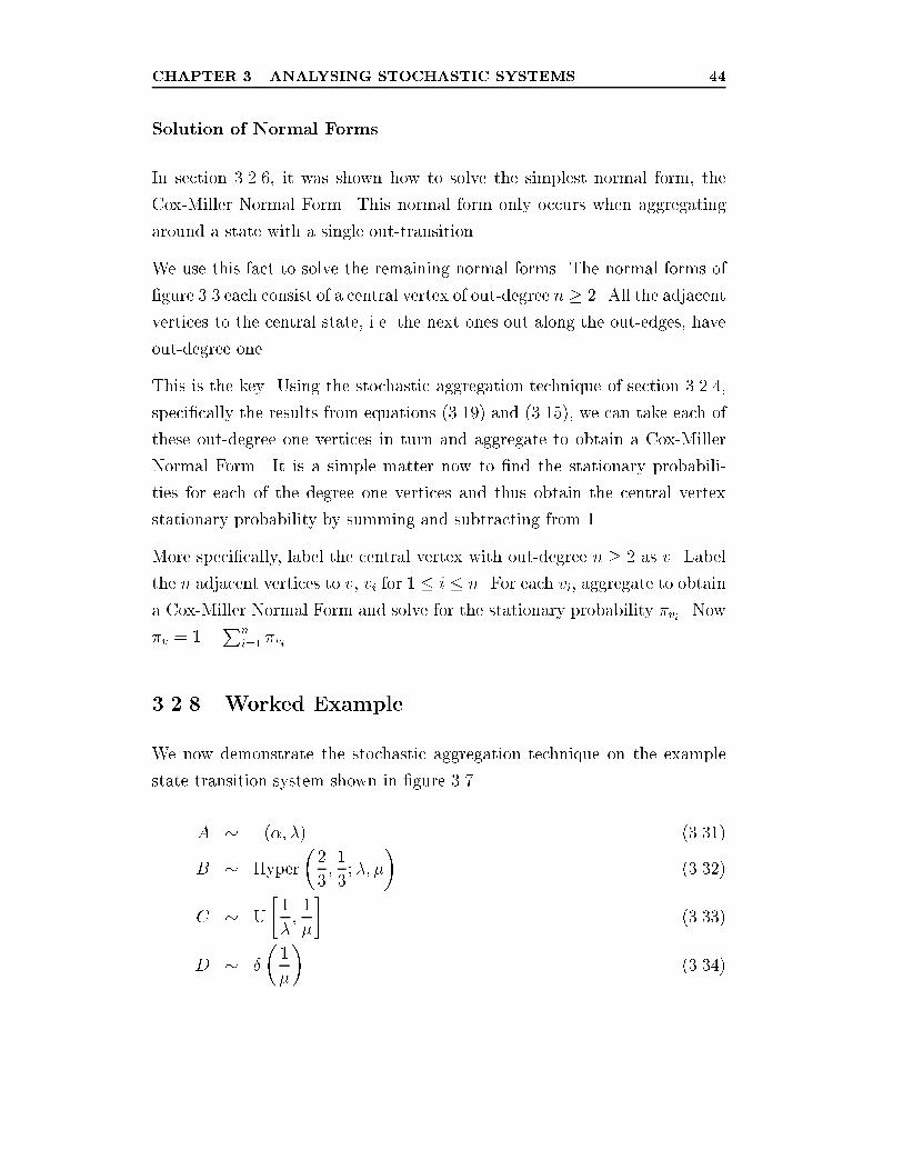
CHAPTER 3. ANALYSING STOCHASTIC SYSTEMS 44
Solution of Normal Forms
In section 3.2.6, it was shown how to solve the simplest normal form, the
Cox-Miller Normal Form. This normal form only occurs when aggregating
around a state with a single out-transition.
We use this fact to solve the remaining normal forms. The normal forms of
�gure 3.3 each consist of a central vertex of out-degree n � 2. All the adjacent
vertices to the central state, i.e. the next ones out along the out-edges, have
out-degree one.
This is the key. Using the stochastic aggregation technique of section 3.2.4,
speci�cally the results from equations (3.19) and (3.15), we can take each of
these out-degree one vertices in turn and aggregate to obtain a Cox-Miller
Normal Form. It is a simple matter now to �nd the stationary probabili-
ties for each of the degree one vertices and thus obtain the central vertex
stationary probability by summing and subtracting from 1.
More speci�cally, label the central vertex with out-degree n � 2 as v. Label
the n adjacent vertices to v, vi for 1 � i � n. For each vi, aggregate to obtain
a Cox-Miller Normal Form and solve for the stationary probability �vi . Now
�v = 1�Pni=1 �vi .
3.2.8 Worked Example
We now demonstrate the stochastic aggregation technique on the example
state transition system shown in �gure 3.7.
A � �(�; �) (3.31)
B � Hyper
�2
3;1
3;�; �
�(3.32)
C � U
�1
�;1
�
�(3.33)
D � �
�1
�
�(3.34)
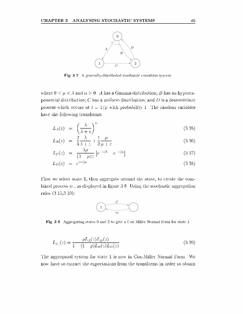
CHAPTER 3. ANALYSING STOCHASTIC SYSTEMS 45
Fig. 3.7. A generally-distributed stochastic transition system.
where 0 < � < � and � > 0. A has a Gamma distribution; B has an hyperex-
ponential distribution; C has a uniform distribution; and D is a deterministic
process which occurs at t = 1=� with probability 1. The random variables
have the following transforms:
LA(z) =
��
� + z
��(3.35)
LB(z) =2
3
�
�+ z+1
3
�
�+ z(3.36)
LC(z) =��
(�� �)z�e�z=� � e�z=�� (3.37)
LD(z) = e�z=� (3.38)
First we select state 1, then aggregate around the state, to create the com-
bined process 1, as displayed in �gure 3.8. Using the stochastic aggregation
rules (3.15,3.19):
Fig. 3.8. Aggregating states 0 and 2 to give a Cox-Miller Normal Form for state 1.
L 1(z) =pLA(z)LD(z)
1� (1� p)LB(z)LD(z) (3.39)
The aggregated system for state 1 is now in Cox-Miller Normal Form. We
now have to extract the expectations from the transforms in order to obtain
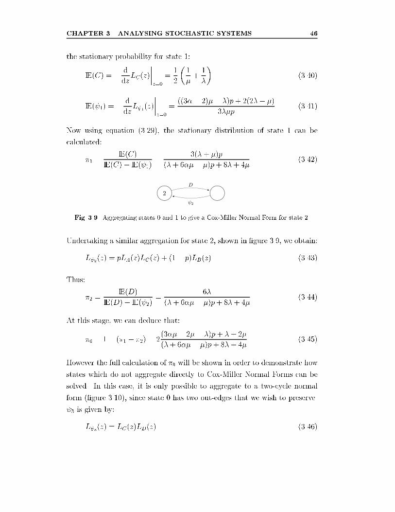
CHAPTER 3. ANALYSING STOCHASTIC SYSTEMS 46
the stationary probability for state 1:
IE(C) = � d
dzLC(z)
����z=0
=1
2
�1
�+
1
�
�(3.40)
IE( 1) = � d
dzL 1(z)
����z=0
=((3�� 2)�� �)p+ 2(2�+ �)
3��p(3.41)
Now using equation (3.29), the stationary distribution of state 1 can be
calculated:
�1 =IE(C)
IE(C) + IE( 1)=
3(�+ �)p
(�+ 6��� �)p+ 8�+ 4�(3.42)
Fig. 3.9. Aggregating states 0 and 1 to give a Cox-Miller Normal Form for state 2.
Undertaking a similar aggregation for state 2, shown in �gure 3.9, we obtain:
L 2(z) = pLA(z)LC(z) + (1� p)LB(z) (3.43)
Thus:
�2 =IE(D)
IE(D) + IE( 2)=
6�
(�+ 6��� �)p+ 8�+ 4�(3.44)
At this stage, we can deduce that:
�0 = 1� (�1 + �2) = 2(3��� 2�� �)p+ �+ 2�
(�+ 6��� �)p+ 8�+ 4�(3.45)
However the full calculation of �0 will be shown in order to demonstrate how
states which do not aggregate directly to Cox-Miller Normal Forms can be
solved. In this case, it is only possible to aggregate to a two-cycle normal
form (�gure 3.10), since state 0 has two out-edges that we wish to preserve.
3 is given by:
L 3(z) = LC(z)LD(z) (3.46)
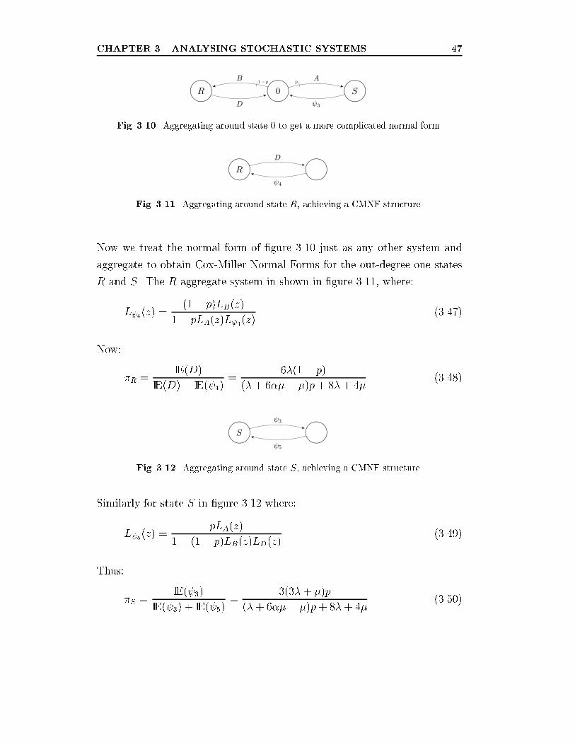
CHAPTER 3. ANALYSING STOCHASTIC SYSTEMS 47
Fig. 3.10. Aggregating around state 0 to get a more complicated normal form.
Fig. 3.11. Aggregating around state R, achieving a CMNF structure.
Now we treat the normal form of �gure 3.10 just as any other system and
aggregate to obtain Cox-Miller Normal Forms for the out-degree one states
R and S. The R aggregate system in shown in �gure 3.11, where:
L 4(z) =(1� p)LB(z)
1� pLA(z)L 3(z)(3.47)
Now:
�R =IE(D)
IE(D) + IE( 4)=
6�(1� p)(�+ 6��� �)p+ 8�+ 4�
(3.48)
Fig. 3.12. Aggregating around state S, achieving a CMNF structure.
Similarly for state S in �gure 3.12 where:
L 5(z) =pLA(z)
1� (1� p)LB(z)LD(z) (3.49)
Thus:
�S =IE( 3)
IE( 3) + IE( 5)=
3(3�+ �)p
(�+ 6��� �)p+ 8�+ 4�(3.50)
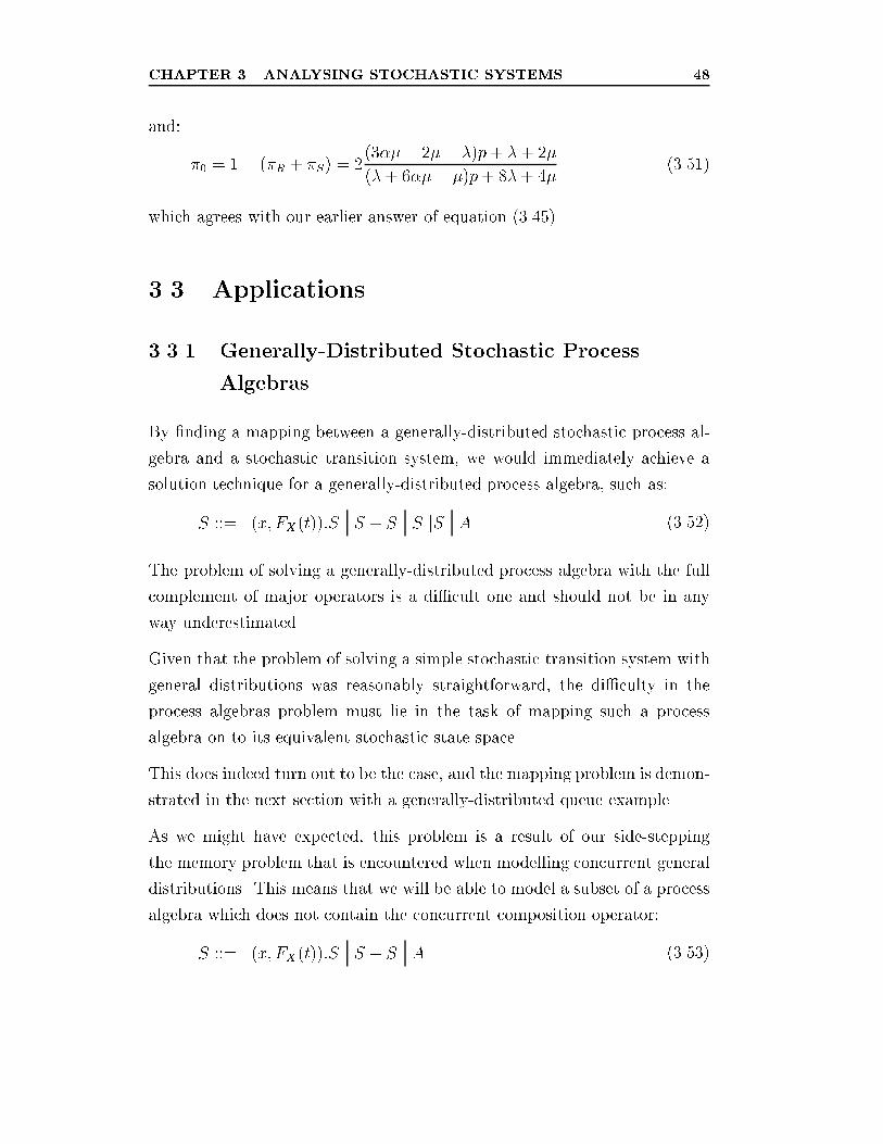
CHAPTER 3. ANALYSING STOCHASTIC SYSTEMS 48
and:
�0 = 1� (�R + �S) = 2(3��� 2�� �)p+ �+ 2�
(�+ 6��� �)p+ 8�+ 4�(3.51)
which agrees with our earlier answer of equation (3.45).
3.3 Applications
3.3.1 Generally-Distributed Stochastic Process
Algebras
By �nding a mapping between a generally-distributed stochastic process al-
gebra and a stochastic transition system, we would immediately achieve a
solution technique for a generally-distributed process algebra, such as:
S ::= (x; FX(t)):S S + S SjjS A (3.52)
The problem of solving a generally-distributed process algebra with the full
complement of major operators is a di�cult one and should not be in any
way underestimated.
Given that the problem of solving a simple stochastic transition system with
general distributions was reasonably straightforward, the di�culty in the
process algebras problem must lie in the task of mapping such a process
algebra on to its equivalent stochastic state space.
This does indeed turn out to be the case, and the mapping problem is demon-
strated in the next section with a generally-distributed queue example.
As we might have expected, this problem is a result of our side-stepping
the memory problem that is encountered when modelling concurrent general
distributions. This means that we will be able to model a subset of a process
algebra which does not contain the concurrent composition operator:
S ::= (x; FX(t)):S S + S A (3.53)
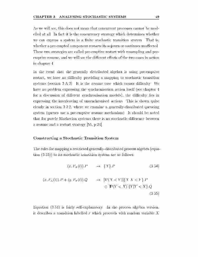
CHAPTER 3. ANALYSING STOCHASTIC SYSTEMS 49
As we will see, this does not mean that concurrent processes cannot be mod-
elled at all. In fact it is the concurrency strategy which determines whether
we can express a system in a �nite stochastic transition system. That is,
whether a pre-empted component restarts its sojourn or continues una�ected.
These two strategies are called pre-emptive restart with resampling and pre-
emptive resume, and we will see the di�erent e�ects of the two cases in action
in chapter 4.
In the event that the generally distributed algebra is using pre-emptive
restart, we have no di�culty providing a mapping to stochastic transition
systems (section 3.A.3). It is the resume case which causes di�culty. We
have no problem expressing the synchronisation action itself (see chapter 4
for a discussion of di�erent synchronisation models), the di�culty lies in
expressing the interleaving of unsynchronised actions. This is shown quite
clearly in section 3.3.2, where we examine a generally-distributed queueing
system (queues use a pre-emptive resume mechanism). It should be noted
that for purely Markovian systems there is no stochastic di�erence between
a resume and a restart strategy [55, p.24].
Constructing a Stochastic Transition System
The rules for mapping a restricted generally-distributed process algebra (equa-
tion (3.53)) to its stochastic transition system are as follows:
(x; FX(t)):P ���! fXg:P (3.54)
(x; FX(t)):P + (y; FY (t)):Q ���! [IP(X < Y )]fXjX < Y g:P� [IP(Y < X)]fY jY < Xg:Q
(3.55)
Equation (3.54) is fairly self-explanatory. In the process algebra version,
it describes a transition labelled x which proceeds with random variable X
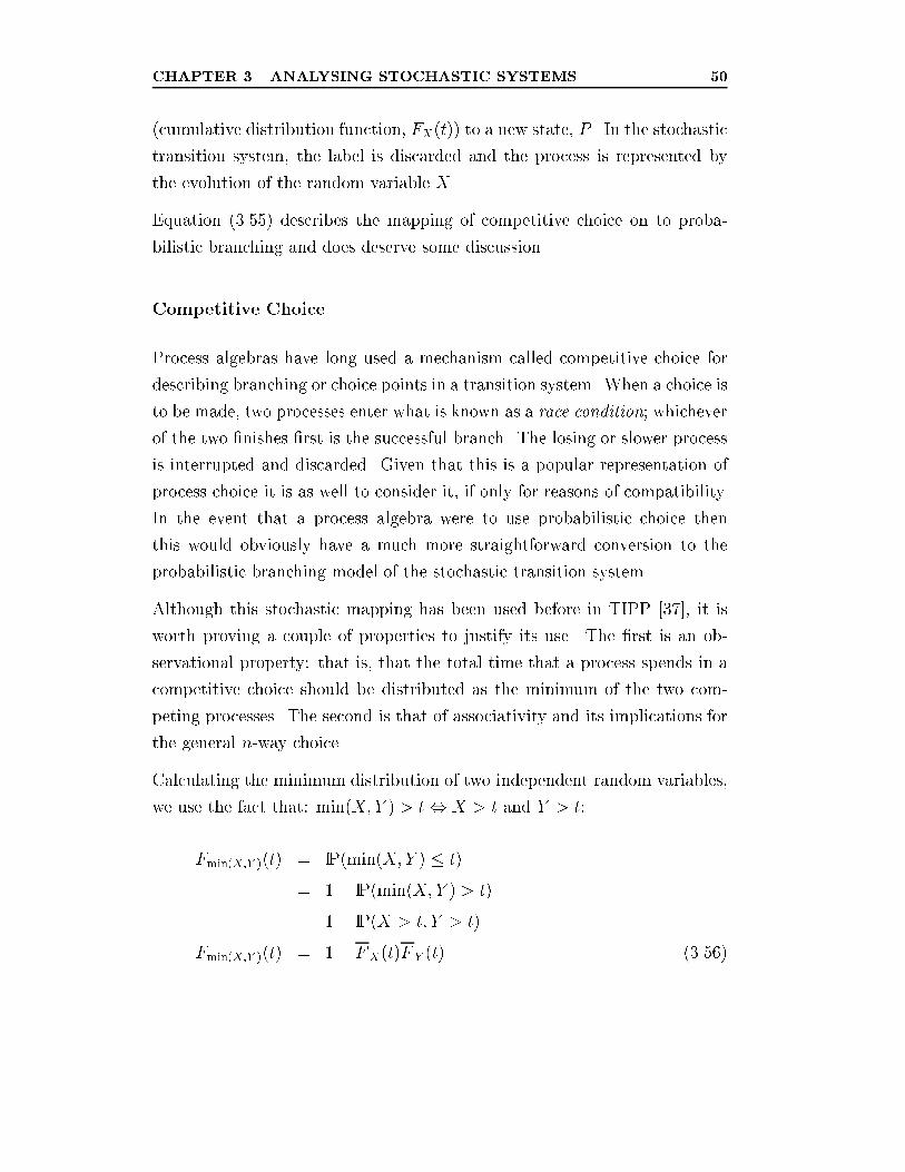
CHAPTER 3. ANALYSING STOCHASTIC SYSTEMS 50
(cumulative distribution function, FX(t)) to a new state, P . In the stochastic
transition system, the label is discarded and the process is represented by
the evolution of the random variable X.
Equation (3.55) describes the mapping of competitive choice on to proba-
bilistic branching and does deserve some discussion.
Competitive Choice
Process algebras have long used a mechanism called competitive choice for
describing branching or choice points in a transition system. When a choice is
to be made, two processes enter what is known as a race condition; whichever
of the two �nishes �rst is the successful branch. The losing or slower process
is interrupted and discarded. Given that this is a popular representation of
process choice it is as well to consider it, if only for reasons of compatibility.
In the event that a process algebra were to use probabilistic choice then
this would obviously have a much more straightforward conversion to the
probabilistic branching model of the stochastic transition system.
Although this stochastic mapping has been used before in TIPP [37], it is
worth proving a couple of properties to justify its use. The �rst is an ob-
servational property: that is, that the total time that a process spends in a
competitive choice should be distributed as the minimum of the two com-
peting processes. The second is that of associativity and its implications for
the general n-way choice.
Calculating the minimum distribution of two independent random variables,
we use the fact that: min(X; Y ) > t, X > t and Y > t:
Fmin(X;Y )(t) = IP(min(X; Y ) � t)
= 1� IP(min(X; Y ) > t)
= 1� IP(X > t; Y > t)
Fmin(X;Y )(t) = 1� FX(t)F Y (t) (3.56)
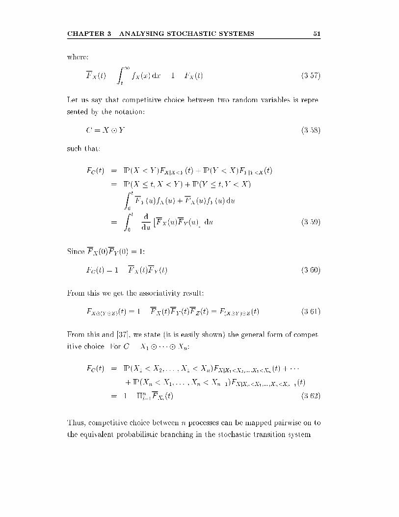
CHAPTER 3. ANALYSING STOCHASTIC SYSTEMS 51
where:
FX(t) =
Z 1
t
fX(x) dx = 1� FX(t) (3.57)
Let us say that competitive choice between two random variables is repre-
sented by the notation:
C = X � Y (3.58)
such that:
FC(t) = IP(X < Y )FXjX<Y (t) + IP(Y < X)FY jY <X(t)
= IP(X � t; X < Y ) + IP(Y � t; Y < X)
=
Z t
0
F Y (u)fX(u) + FX(u)fY (u) du
=
Z t
0
� d
du
�FX(u)F Y (u)
�du (3.59)
Since FX(0)F Y (0) = 1:
FC(t) = 1� FX(t)F Y (t) (3.60)
From this we get the associativity result:
FX�(Y �Z)(t) = 1� FX(t)F Y (t)FZ(t) = F(X�Y )�Z(t) (3.61)
From this and [37], we state (it is easily shown) the general form of compet-
itive choice. For C = X1 � � � � �Xn:
FC(t) = IP(X1 < X2; : : : ; X1 < Xn)FXjX1<X2;::: ;X1<Xn(t) + � � �
+ IP(Xn < X1; : : : ; Xn < Xn�1)FXjXn<X1;::: ;Xn<Xn�1(t)
= 1� �ni=1FXi
(t) (3.62)
Thus, competitive choice between n processes can be mapped pairwise on to
the equivalent probabilistic branching in the stochastic transition system.
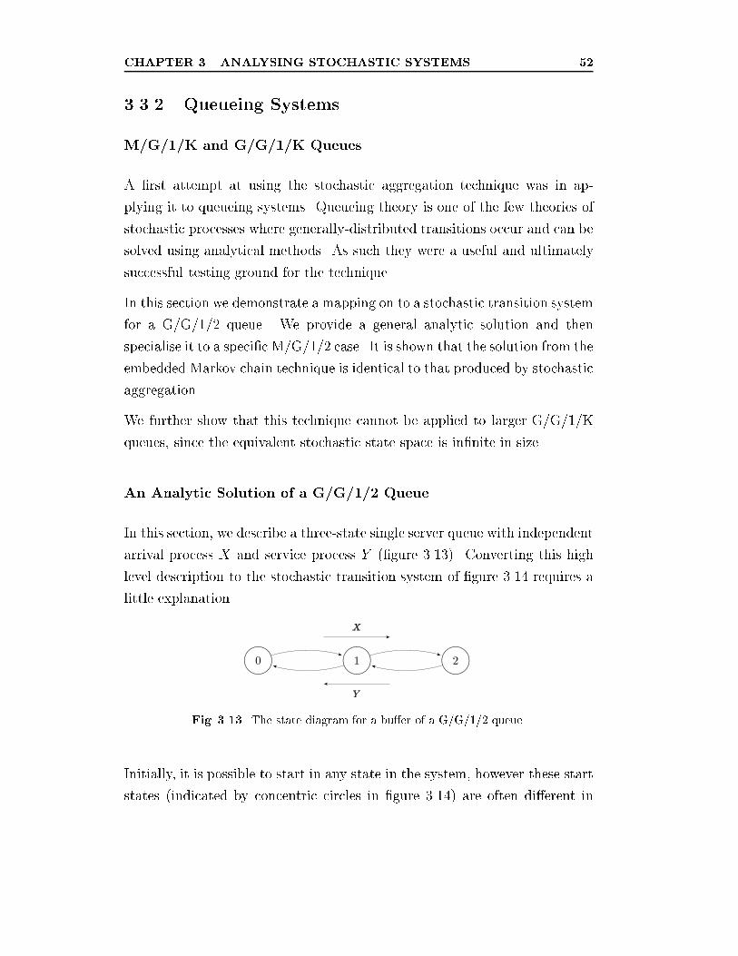
CHAPTER 3. ANALYSING STOCHASTIC SYSTEMS 52
3.3.2 Queueing Systems
M/G/1/K and G/G/1/K Queues
A �rst attempt at using the stochastic aggregation technique was in ap-
plying it to queueing systems. Queueing theory is one of the few theories of
stochastic processes where generally-distributed transitions occur and can be
solved using analytical methods. As such they were a useful and ultimately
successful testing ground for the technique.
In this section we demonstrate a mapping on to a stochastic transition system
for a G/G/1/2 queue. We provide a general analytic solution and then
specialise it to a speci�c M/G/1/2 case. It is shown that the solution from the
embedded Markov chain technique is identical to that produced by stochastic
aggregation.
We further show that this technique cannot be applied to larger G/G/1/K
queues, since the equivalent stochastic state space is in�nite in size.
An Analytic Solution of a G/G/1/2 Queue
In this section, we describe a three-state single server queue with independent
arrival process X and service process Y (�gure 3.13). Converting this high
level description to the stochastic transition system of �gure 3.14 requires a
little explanation.
Fig. 3.13. The state diagram for a bu�er of a G/G/1/2 queue.
Initially, it is possible to start in any state in the system, however these start
states (indicated by concentric circles in �gure 3.14) are often di�erent in
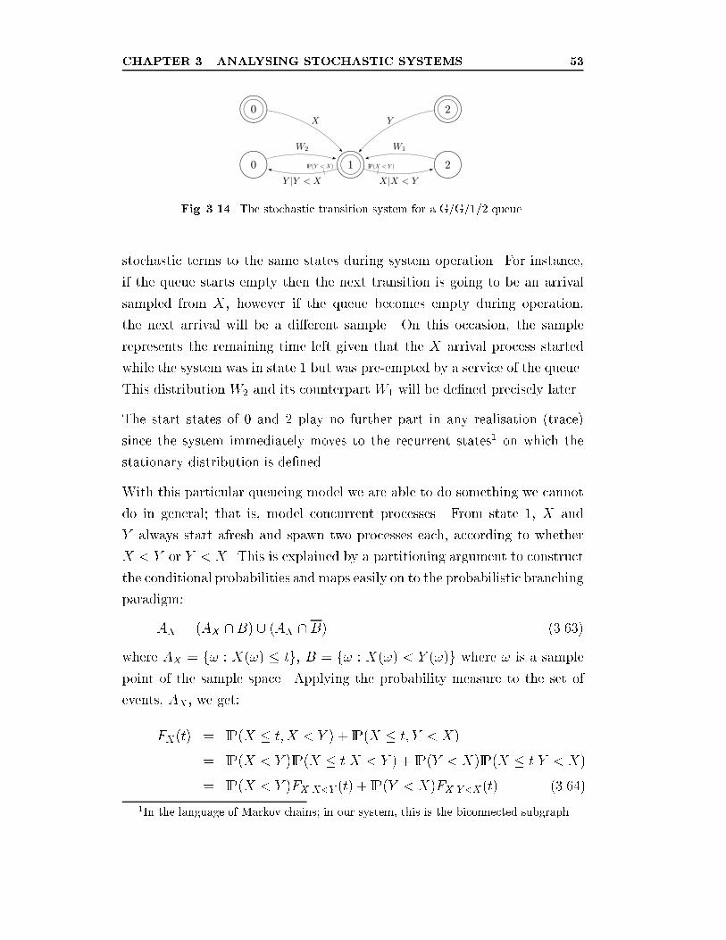
CHAPTER 3. ANALYSING STOCHASTIC SYSTEMS 53
Fig. 3.14. The stochastic transition system for a G/G/1/2 queue.
stochastic terms to the same states during system operation. For instance,
if the queue starts empty then the next transition is going to be an arrival
sampled from X, however if the queue becomes empty during operation,
the next arrival will be a di�erent sample. On this occasion, the sample
represents the remaining time left given that the X arrival process started
while the system was in state 1 but was pre-empted by a service of the queue.
This distribution W2 and its counterpart W1 will be de�ned precisely later.
The start states of 0 and 2 play no further part in any realisation (trace)
since the system immediately moves to the recurrent states1 on which the
stationary distribution is de�ned.
With this particular queueing model we are able to do something we cannot
do in general; that is, model concurrent processes. From state 1, X and
Y always start afresh and spawn two processes each, according to whether
X < Y or Y < X. This is explained by a partitioning argument to construct
the conditional probabilities and maps easily on to the probabilistic branching
paradigm:
AX = (AX \B) [ (AX \ B) (3.63)
where AX = f! : X(!) � tg, B = f! : X(!) < Y (!)g where ! is a sample
point of the sample space. Applying the probability measure to the set of
events, AX , we get:
FX(t) = IP(X � t; X < Y ) + IP(X � t; Y < X)
= IP(X < Y )IP(X � tjX < Y ) + IP(Y < X)IP(X � tjY < X)
= IP(X < Y )FXjX<Y (t) + IP(Y < X)FXjY <X(t) (3.64)
1In the language of Markov chains; in our system, this is the biconnected subgraph.
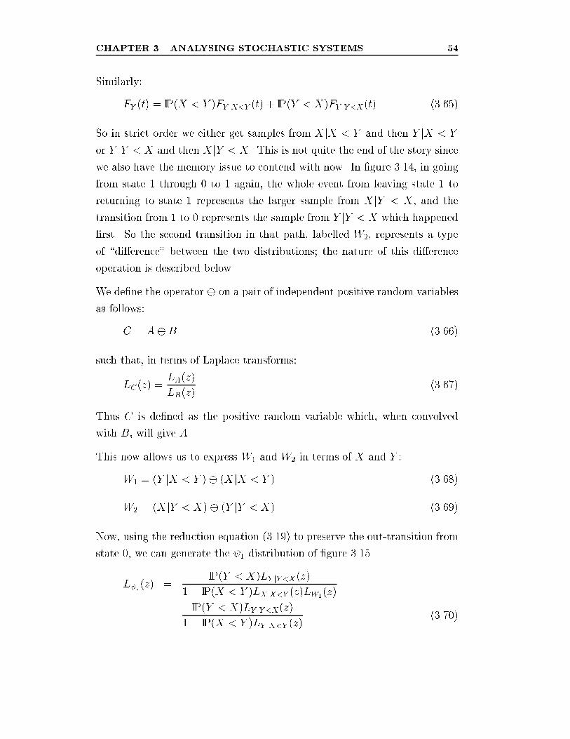
CHAPTER 3. ANALYSING STOCHASTIC SYSTEMS 54
Similarly:
FY (t) = IP(X < Y )FY jX<Y (t) + IP(Y < X)FY jY <X(t) (3.65)
So in strict order we either get samples from XjX < Y and then Y jX < Y
or Y jY < X and then XjY < X. This is not quite the end of the story since
we also have the memory issue to contend with now. In �gure 3.14, in going
from state 1 through 0 to 1 again, the whole event from leaving state 1 to
returning to state 1 represents the larger sample from XjY < X, and the
transition from 1 to 0 represents the sample from Y jY < X which happened
�rst. So the second transition in that path, labelled W2, represents a type
of \di�erence" between the two distributions; the nature of this di�erence
operation is described below.
We de�ne the operator on a pair of independent positive random variables
as follows:
C = AB (3.66)
such that, in terms of Laplace transforms:
LC(z) =LA(z)
LB(z)(3.67)
Thus C is de�ned as the positive random variable which, when convolved
with B, will give A.
This now allows us to express W1 and W2 in terms of X and Y :
W1 = (Y jX < Y ) (XjX < Y ) (3.68)
W2 = (XjY < X) (Y jY < X) (3.69)
Now, using the reduction equation (3.19) to preserve the out-transition from
state 0, we can generate the 1 distribution of �gure 3.15.
L 1(z) =IP(Y < X)LY jY <X(z)
1� IP(X < Y )LXjX<Y (z)LW1(z)
=IP(Y < X)LY jY <X(z)
1� IP(X < Y )LY jX<Y (z)(3.70)
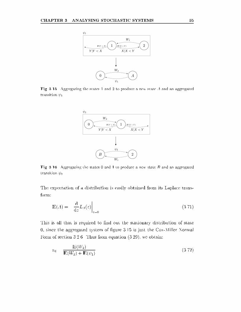
CHAPTER 3. ANALYSING STOCHASTIC SYSTEMS 55
Fig. 3.15. Aggregating the states 1 and 2 to produce a new state A and an aggregated
transition 1.
Fig. 3.16. Aggregating the states 0 and 1 to produce a new state B and an aggregated
transition 2.
The expectation of a distribution is easily obtained from its Laplace trans-
form:
IE(A) = � d
dzLA(z)
����z=0
(3.71)
This is all that is required to �nd out the stationary distribution of state
0, since the aggregated system of �gure 3.15 is just the Cox-Miller Normal
Form of section 3.2.6. Thus from equation (3.29), we obtain:
�0 =IE(W2)
IE(W2) + IE( 1)(3.72)
CHAPTER 3. ANALYSING STOCHASTIC SYSTEMS 56
Similarly, reducing the system to preserve state 2, we get the aggregated
transition, 2 in �gure 3.16:
L 2(z) =IP(X < Y )LXjX<Y (z)
1� IP(Y < X)LXjY <X(z)(3.73)
Now having obtained a second Cox-Miller Normal Form, �2 follows:
�2 =IE(W1)
IE(W1) + IE( 2)(3.74)
Finally:
�1 = 1� (�0 + �2) (3.75)
M/G/1/2 Example
Specialising the G/G/1/2 result to use a Markovian arrival process simpli�es
some of the expressions. Importantly the end result can be checked using
standard M/G/1/K queueing techniques.
Let the arrival process X and service process Y be de�ned as follows:
fX(t) = �e��t (3.76)
fY (t) = �e��t + �e��t � (�+ �)e�(�+�)t (3.77)
Now, we can specify the exact transition distributions of �gure 3.14 and thus,
from equations (3.72, 3.75, 3.74), the stationary distribution of the queue:
�0 = �2�2(� + �)(�+ � + 2�)� (3.78)
�1 = ���(�+ �)((�+ � + �)2 � ��)� (3.79)
�2 = ((�2 + �� + �2)�2 + (� + �)(2�2 + �� + 2�2)�
+ �4 + 2�3� + �2�2 + 2��3 + �4)� (3.80)
CHAPTER 3. ANALYSING STOCHASTIC SYSTEMS 57
where:
� =�(�2 + �� + �2)�4 + 2(�+ �)(�2 + �� + �2)�3
+ (�2 + �� + �2)(�2 + 3�� + �2)�2
+ ��(�+ �)(�2 + 3�� + �2)�+ �2�2(�+ �)2��1
(3.81)
These results are identical to those obtained using embedded Markov chain
techniques from traditional queueing theory [23, 66, 38].
Larger G/G/1/K Queues
So, can the same techniques be applied to larger general queueing systems?
The answer, probably unsurprisingly, is no; not directly at least. To see
why, we need to look at how the processes can interleave. Figure 3.17 shows
an interleaving for a G/G/1/3 queue. The synchronising states (states from
which both arrival and service distributions start simultaneously) are marked
by concentric circles.
This is not the stochastic state space of other diagrams, it represents instead
how the processes interleave by showing how many services (or arrivals) have
occurred while an arrival (or service) has still to occur. It is a distinct diagram
from that of the normal queue bu�er representation. For example, observe
that there are distinct instances of the state with one item in the queue: one
instance when both the arrival and service processes start simultaneously and
one when the service process Y is starting again (having just occurred) while
the arrival process X has been running for a single service time. Whether the
arrival process happens next depends now on a race between a fresh service
process and a one-service-time-old arrival process.
However, as already stated, this is not a stochastic transition system either.
The reason is that although this represents a consistent interleaving, the
distributions of the individual edges are not necessarily the same each time
that edge is traversed. Speci�cally, for the cycle between 2a and 1b, each time
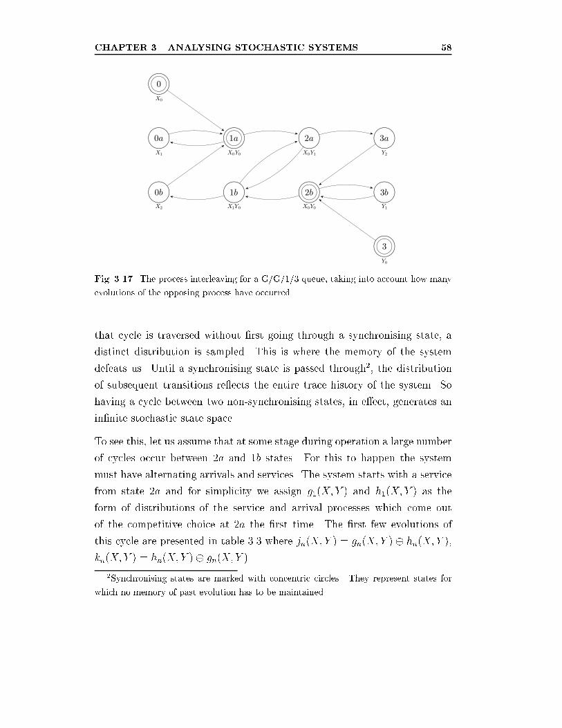
CHAPTER 3. ANALYSING STOCHASTIC SYSTEMS 58
Fig. 3.17. The process interleaving for a G/G/1/3 queue, taking into account how many
evolutions of the opposing process have occurred.
that cycle is traversed without �rst going through a synchronising state, a
distinct distribution is sampled. This is where the memory of the system
defeats us. Until a synchronising state is passed through2, the distribution
of subsequent transitions re ects the entire trace history of the system. So
having a cycle between two non-synchronising states, in e�ect, generates an
in�nite stochastic state space.
To see this, let us assume that at some stage during operation a large number
of cycles occur between 2a and 1b states. For this to happen the system
must have alternating arrivals and services. The system starts with a service
from state 2a and for simplicity we assign g1(X; Y ) and h1(X; Y ) as the
form of distributions of the service and arrival processes which come out
of the competitive choice at 2a the �rst time. The �rst few evolutions of
this cycle are presented in table 3.3 where jn(X; Y ) = gn(X; Y ) hn(X; Y ),kn(X; Y ) = hn(X; Y ) gn(X; Y ).
2Synchronising states are marked with concentric circles. They represent states for
which no memory of past evolution has to be maintained.
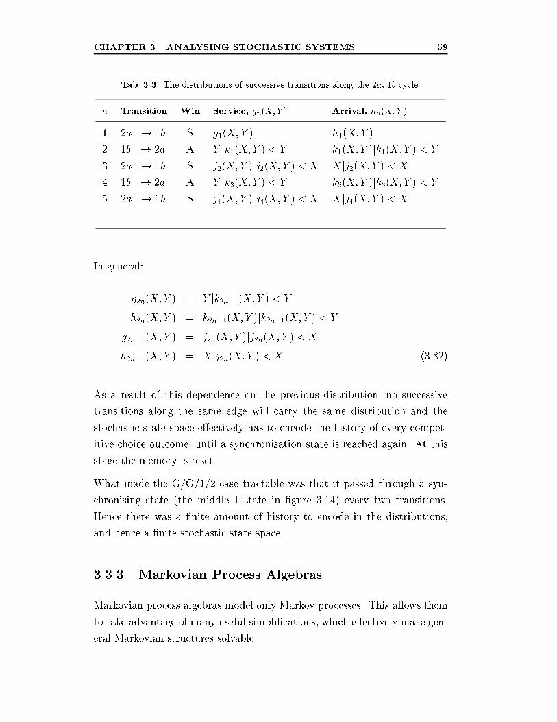
CHAPTER 3. ANALYSING STOCHASTIC SYSTEMS 59
Tab. 3.3. The distributions of successive transitions along the 2a, 1b cycle.
n Transition Win Service, gn(X;Y ) Arrival, hn(X;Y )
1 2a �! 1b S g1(X; Y ) h1(X; Y )
2 1b �! 2a A Y jk1(X; Y ) < Y k1(X; Y )jk1(X; Y ) < Y
3 2a �! 1b S j2(X; Y )jj2(X; Y ) < X Xjj2(X; Y ) < X
4 1b �! 2a A Y jk3(X; Y ) < Y k3(X; Y )jk3(X; Y ) < Y
5 2a �! 1b S j4(X; Y )jj4(X; Y ) < X Xjj4(X; Y ) < X...
In general:
g2n(X; Y ) = Y jk2n�1(X; Y ) < Y
h2n(X; Y ) = k2n�1(X; Y )jk2n�1(X; Y ) < Y
g2n+1(X; Y ) = j2n(X; Y )jj2n(X; Y ) < X
h2n+1(X; Y ) = Xjj2n(X; Y ) < X (3.82)
As a result of this dependence on the previous distribution, no successive
transitions along the same edge will carry the same distribution and the
stochastic state space e�ectively has to encode the history of every compet-
itive choice outcome, until a synchronisation state is reached again. At this
stage the memory is reset.
What made the G/G/1/2 case tractable was that it passed through a syn-
chronising state (the middle 1 state in �gure 3.14) every two transitions.
Hence there was a �nite amount of history to encode in the distributions,
and hence a �nite stochastic state space.
3.3.3 Markovian Process Algebras
Markovian process algebras model only Markov processes. This allows them
to take advantage of many useful simpli�cations, which e�ectively make gen-
eral Markovian structures solvable.
CHAPTER 3. ANALYSING STOCHASTIC SYSTEMS 60
It has already been shown that competitive choice can, in the generally-
distributed case, be mapped on to the probabilistic branching of a stochastic
transition system. Obviously competitive choice of Markov processes can be
similarly mapped. The important di�erence to note from that of generally-
distributed SPAs and generally-distributed queueing systems, is that, in a
Markovian system, an expansion law exists for parallel composition.
For PEPA an expansion law is found in [52]; for MTIPP, one can be found
in [47].
The expansion law for PEPA, for instance, maps the di�erent components of
the composition on to a �nite Markovian state space consisting of competitive
choices, in a similar fashion to CCS. We are in the luxurious position of saying
that the hard work has therefore been done for us. This mapping represents
a proof that the stochastic aggregation technique can be used directly to
solve any Markovian process algebra.
So long as the parallel composition has been removed using the expansion
law mentioned, we are able to map the components of a typical MPA on to
its stochastic transition system loosely as follows:
(x; �):P ���! fXg:P (3.83)
(x; �):P + (y; �):Q ���!�
�
�+ �
�fZg:P �
��
�+ �
�fZg:Q (3.84)
where X � exp(�), Y � exp(�) and Z � exp(�+ �).
The immediate corollary of this is that an MPA no longer has to proceed via
a Markov chain solution technique in order to obtain its stationary distri-
bution. Since it can be mapped on to a �nite stochastic transition system,
the stochastic aggregation technique can be applied. An example of this is
shown below.
CHAPTER 3. ANALYSING STOCHASTIC SYSTEMS 61
Reward Structures
On the surface, the major bene�t is that the stationary distribution can be
generated in a state-wise fashion. This has a nice e�ect for calculating reward
structures and performance measures, for MPAs. If a reward structure is
sparse, i.e. it only rewards a few states, then the aggregation technique can
be used to �nd only the stationary probabilities of the required states. Using
traditional techniques, the entire model would have to be solved in order to
calculate maybe only a few stationary values.
However, key to this is whether we can devise an algorithm which can gen-
erate a single element of the steady-state probability in less time than it
would take to solve the CTMC. The proof method of section 3.2.7 is clearly
not a good candidate for this. In fact, we suspect that the best we might
be able to do is construct a matrix of Laplacian functions representing the
transition distributions and then invert it in such a way as to get the overall
path Laplacian function, representing the aggregated return path of the Cox-
Miller Normal Form. Preliminary results indicate that this method would
require inversion of an n�1�n�1 matrix for each of the n states. This rep-
resents a small practical saving per state over solving the complete CTMC,
although the O-complexity is clearly the same.
A second property of the method is that it is a progressive technique. It will
generate the distribution, a result at a time, rather than the entire solution
in one go. This may well make it amenable to lazy implementation.
Example
As an example of solving a Markovian Process Algebra system, we examine
the PEPA resource usage model of [52], de�ned in �gure 3.18.
The cooperation is removed using the expansion law of [52], giving the state
diagram of �gure 3.19. In �gure 3.20, states X1 and X3 have been aggregated
to give state A1 and states X2 and X3 have been aggregated to give state A2.
This �rst stochastic aggregation man�uvre reduces the transition system to
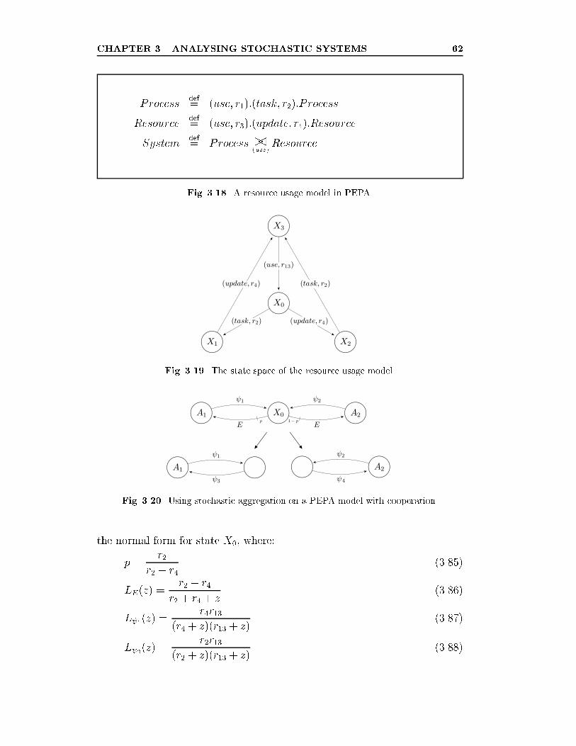
CHAPTER 3. ANALYSING STOCHASTIC SYSTEMS 62
Processdef= (use; r1):(task; r2):P rocess
Resourcedef= (use; r3):(update; r4):Resource
Systemdef= Process ��
fusegResource
Fig. 3.18. A resource usage model in PEPA.
Fig. 3.19. The state space of the resource usage model.
Fig. 3.20. Using stochastic aggregation on a PEPA model with cooperation.
the normal form for state X0, where:
p =r2
r2 + r4(3.85)
LE(z) =r2 + r4
r2 + r4 + z(3.86)
L 1(z) =r4r13
(r4 + z)(r13 + z)(3.87)
L 2(z) =r2r13
(r2 + z)(r13 + z)(3.88)
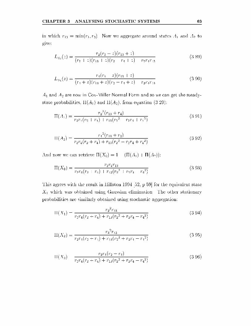
CHAPTER 3. ANALYSING STOCHASTIC SYSTEMS 63
in which r13 = min(r1; r3). Now we aggregate around states A1 and A2 to
give:
L 3(z) =r2(r2 + z)(r13 + z)
(r2 + z)(r13 + z)(r2 + r4 + z)� r2r4r13 (3.89)
L 4(z) =r4(r4 + z)(r13 + z)
(r4 + z)(r13 + z)(r2 + r4 + z)� r2r4r13 (3.90)
A1 and A2 are now in Cox-Miller Normal Form and so we can get the steady-
state probabilities, �(A1) and �(A2), from equation (3.29):
�(A1) =r2
2(r13 + r4)
r2r4(r2 + r4) + r13(r22 + r2r4 + r42)(3.91)
�(A2) =r4
2(r13 + r2)
r2r4(r2 + r4) + r13(r22 + r2r4 + r42)(3.92)
And now we can retrieve �(X0) = 1� (�(A1) + �(A2)):
�(X0) =r2r4r13
r2r4(r2 + r4) + r13(r22 + r2r4 + r42)(3.93)
This agrees with the result in Hillston 1994 [52, p.59] for the equivalent state
X1 which was obtained using Gaussian elimination. The other stationary
probabilities are similarly obtained using stochastic aggregation:
�(X1) =r2
2r13r2r4(r2 + r4) + r13(r22 + r2r4 + r42)
(3.94)
�(X2) =r4
2r13r2r4(r2 + r4) + r13(r22 + r2r4 + r42)
(3.95)
�(X3) =r2r4(r2 + r4)
r2r4(r2 + r4) + r13(r22 + r2r4 + r42)(3.96)
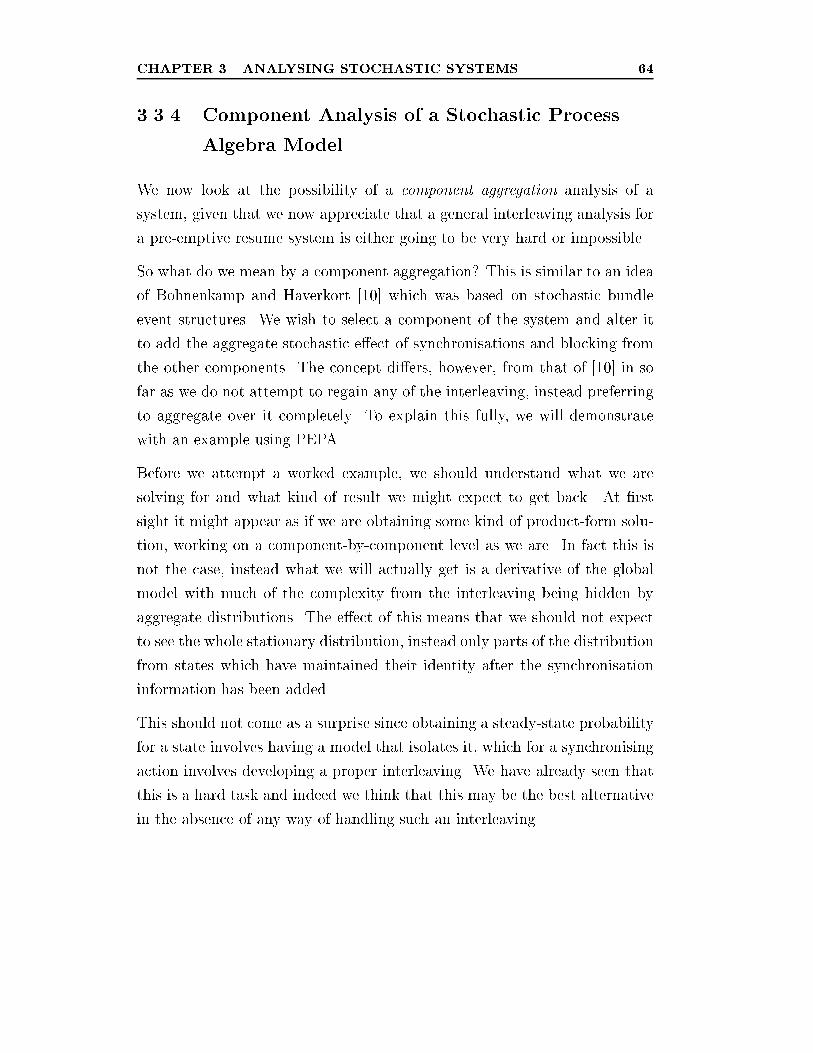
CHAPTER 3. ANALYSING STOCHASTIC SYSTEMS 64
3.3.4 Component Analysis of a Stochastic Process
Algebra Model
We now look at the possibility of a component aggregation analysis of a
system, given that we now appreciate that a general interleaving analysis for
a pre-emptive resume system is either going to be very hard or impossible.
So what do we mean by a component aggregation? This is similar to an idea
of Bohnenkamp and Haverkort [10] which was based on stochastic bundle
event structures. We wish to select a component of the system and alter it
to add the aggregate stochastic e�ect of synchronisations and blocking from
the other components. The concept di�ers, however, from that of [10] in so
far as we do not attempt to regain any of the interleaving, instead preferring
to aggregate over it completely. To explain this fully, we will demonstrate
with an example using PEPA.
Before we attempt a worked example, we should understand what we are
solving for and what kind of result we might expect to get back. At �rst
sight it might appear as if we are obtaining some kind of product-form solu-
tion, working on a component-by-component level as we are. In fact this is
not the case, instead what we will actually get is a derivative of the global
model with much of the complexity from the interleaving being hidden by
aggregate distributions. The e�ect of this means that we should not expect
to see the whole stationary distribution, instead only parts of the distribution
from states which have maintained their identity after the synchronisation
information has been added.
This should not come as a surprise since obtaining a steady-state probability
for a state involves having a model that isolates it, which for a synchronising
action involves developing a proper interleaving. We have already seen that
this is a hard task and indeed we think that this may be the best alternative
in the absence of any way of handling such an interleaving.
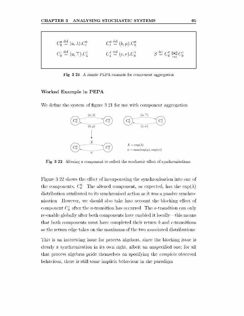
CHAPTER 3. ANALYSING STOCHASTIC SYSTEMS 65
C00
def= (a; �):C0
1 C01
def= (b; �):C0
0
C10
def= (a;>):C1
1 C11
def= (c; �):C1
0 Sdef= C0
0��fag
C10
Fig. 3.21. A simple PEPA example for component aggregation
Worked Example in PEPA
We de�ne the system of �gure 3.21 for use with component aggregation.
Fig. 3.22. Altering a component to re ect the stochastic e�ect of synchronisations.
Figure 3.22 shows the e�ect of incorporating the synchronisation into one of
the components, C00 . The altered component, as expected, has the exp(�)
distribution attributed to its synchronised action as it was a passive synchro-
nisation. However, we should also take into account the blocking e�ect of
component C10 after the a-transition has occurred. The a-transition can only
re-enable globally after both components have enabled it locally|this means
that both components must have completed their return b and c-transitions
so the return edge takes on the maximum of the two associated distributions.
This is an interesting issue for process algebras, since the blocking issue is
clearly a synchronisation in its own right, albeit an unspeci�ed one; for all
that process algebras pride themselves on specifying the complete observed
behaviour, there is still some implicit behaviour in the paradigm.
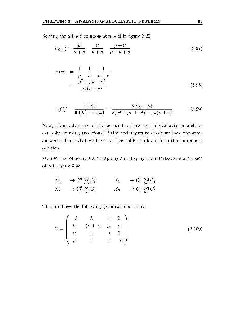
CHAPTER 3. ANALYSING STOCHASTIC SYSTEMS 66
Solving the altered component model in �gure 3.22:
L (z) =�
�+ z+
�
� + z� �+ �
�+ � + z(3.97)
IE( ) =1
�+
1
�� 1
�+ �
=�2 + �� + �2
��(�+ �)(3.98)
�(C00 ) =
IE(X)
IE(X) + IE( )=
��(�+ �)
�(�2 + �� + �2) + ��(�+ �)(3.99)
Now, taking advantage of the fact that we have used a Markovian model, we
can solve it using traditional PEPA techniques to check we have the same
answer and see what we have not been able to obtain from the component
solution.
We use the following state-mapping and display the interleaved state space
of S in �gure 3.23:
X0 ���! C00��fag
C10 X1 ���! C0
1��fag
C11
X2 ���! C00��fag
C11 X3 ���! C0
1��fag
C10
This produces the following generator matrix, G:
G =
0BBBB@�� � 0 0
0 �(�+ �) � �
� 0 �� 0
� 0 0 ��
1CCCCA (3.100)
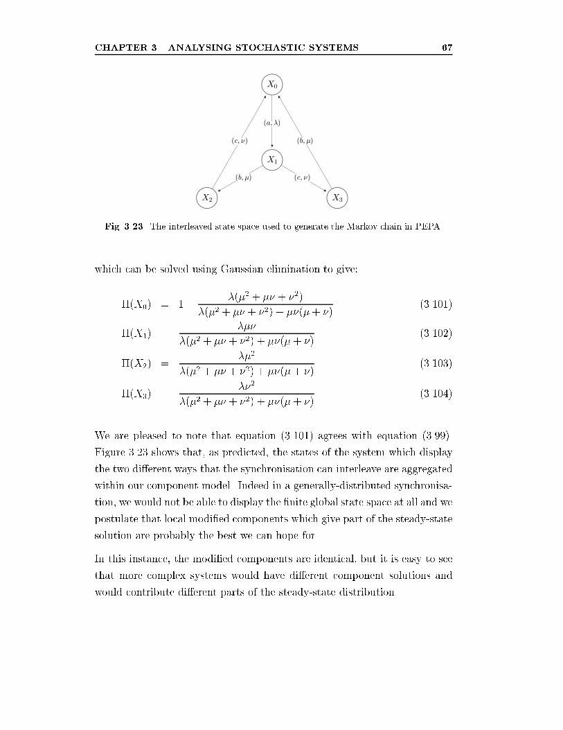
CHAPTER 3. ANALYSING STOCHASTIC SYSTEMS 67
Fig. 3.23. The interleaved state space used to generate the Markov chain in PEPA.
which can be solved using Gaussian elimination to give:
�(X0) = 1� �(�2 + �� + �2)
�(�2 + �� + �2) + ��(�+ �)(3.101)
�(X1) =���
�(�2 + �� + �2) + ��(�+ �)(3.102)
�(X2) =��2
�(�2 + �� + �2) + ��(�+ �)(3.103)
�(X3) =��2
�(�2 + �� + �2) + ��(�+ �)(3.104)
We are pleased to note that equation (3.101) agrees with equation (3.99).
Figure 3.23 shows that, as predicted, the states of the system which display
the two di�erent ways that the synchronisation can interleave are aggregated
within our component model. Indeed in a generally-distributed synchronisa-
tion, we would not be able to display the �nite global state space at all and we
postulate that local modi�ed components which give part of the steady-state
solution are probably the best we can hope for.
In this instance, the modi�ed components are identical, but it is easy to see
that more complex systems would have di�erent component solutions and
would contribute di�erent parts of the steady-state distribution.
CHAPTER 3. ANALYSING STOCHASTIC SYSTEMS 68
As further research, it would be interesting to examine a general framework
for this type of solution method. Although we have analysed a Markovian
system here it would not have been di�cult to tackle such a system with
generally-distributed durations. It is possible that for heavily interdependent
components the complexity of such a technique might be prohibitively high,
but at the very least it might represent another tool in the arsenal to tackle
both the state space explosion and generally-distributed processes.
3.4 Conclusion
In this chapter, we have shown that a class of generally-distributed systems
can be solved. By restating a well-known aggregation technique in the lan-
guage of stochastic process algebras, we can reduce any stochastic transition
system to a normal form for a given state. These normal forms, in turn,
can be solved by using the Cox-Miller Normal Form solution. For each state
of the original system the stationary distribution can be recovered, in a pro-
gressive fashion. This extends a previous result [26] from a purely Markovian
two-state example to a generally-distributed n-state solution technique.
We were able to present an analytical solution to a G/G/1/2 queueing sys-
tem. Further, we demonstrated that the reason that larger queues were not
directly soluble using this technique was that no �nite representation existed
as a stochastic transition system. Since Markovian process algebras have an
expansion law for their concurrent operator, however, it is possible to write
down a �nite stochastic transition system for a general MPA system. This
fact means that we are able to solve MPA systems without having to re-
sort to Markov chains. This represents a small computational saving since it
means that, in order to gain a few stationary probabilities, we no longer have
to solve the entire system. We were also able to map a pre-emptive restart
generally-distributed stochastic process algebra to stochastic transition sys-
tems, through our use of probabilistic operational semantics, de�ned in the
annex 3.A.
CHAPTER 3. ANALYSING STOCHASTIC SYSTEMS 69
The use of an aggregation technique means that we are no longer restricted
to dealing in stationary distributions. The use of Laplace transforms has
the bene�t that we can easily derive the variance of the aggregated states
as well as the mean. This will be useful for deriving reliability information
in chapter 5. In the Markovian process algebra case, in the event that we
require a probability distribution function, we note that there is a useful
Laplace inversion formula by Harrison [39] which would allow us to invert
any aggregate, non-cyclic path of a Markovian system.
The process of aggregation is not one which alters the stochastic behaviour
of a system (unlike, for example, insensitivity), which is essential when we
come to consider more than just steady-state distributions in chapter 5.
We completed the chapter with an example of a component-based analysis
through component aggregation of a process algebra model which abstracted
away from the complexity of the interleaving synchronisation. This may o�er
a performance model solution which avoids state space explosion problems
and is capable of coping with generally-distributed evolutions. It may be pos-
sible to develop a general framework for steady-state solution of stochastic
process algebras about such a technique; however this thesis is concerned pre-
dominantly with reliability rather than performance modelling at this stage.
It is recognised, though, that a previous attempt at such a method [10] in a
di�erent stochastic framework had complexity di�culties and that this might
well be a problem for this technique too. It is worth further investigation|
especially in the area of bounding solutions for performance models.
CHAPTER 3. ANALYSING STOCHASTIC SYSTEMS 70
Annex
3.A Probabilistic Operational Semantics of
Stochastic Process Algebras
In this annex, we demonstrate the mapping of three stochastic process al-
gebra models to their underlying stochastic transition systems. We do this
by introducing a slightly modi�ed form of operational semantics to that of
Plotkin [82]. In order to express the probabilistic nature of the stochastic
evolutions we need to employ a form of probabilistic operational semantics.
Operational semantics are usually presented as in �gure 3.24. An individual
rule is translated as: from the clause above the line, we can infer the resulting
clause below the line, subject to the side conditions (if any).
The probabilistic operational semantics only extends the functional version
by adding probabilities, for uncertain operation. So in �gure 3.25, we inter-
pret the competitive choice rule as: if P(a;�)�! P 0 and Q
(b;�)�! Q0 then we can
infer that with probability �=(� + �), P + Q(a;�+�)���! P 0 or with probability
�=(�+�), P+Q(a;�+�)���! Q0. This embodies perfectly the competitive nature of
the race condition which is missing from the equivalent functional de�nition.
3.A.1 PEPA Operational Semantics
Figure 3.24 shows the traditional operational semantic de�nition of PEPA
reproduced from [55], presented in the style of [82] for comparison.
Figure 3.25 shows the probabilistic operational semantic de�nition of PEPA,
which can capture more of the behavioural features of the stochastic lan-
guage, such as: the probabilistic nature of competitive choice, the actual
interleaving of non-synchronising actions in the pre-emptive resume/restart
cooperation and blocking cooperation. The active synchronisation model
CHAPTER 3. ANALYSING STOCHASTIC SYSTEMS 71
remains unchanged. The de�nitions of constant and hiding constructs are
identical to those in �gure 3.24.
3.A.2 MTIPP Operational Semantics
Figure 3.26 shows the probabilistic operational semantic de�nition of MTIPP.
This is largely the same as for PEPA; but note the di�erence in the ac-
tive synchronisation model, here called scaling factor synchronisation. This
di�erence in Markovian synchronisation is the subject of further study in
chapter 4.
3.A.3 Operational Semantics of a GDSPA
Figure 3.27 shows the probabilistic operational semantic de�nition for a
generally-distributed stochastic process algebra with pre-emptive restart. As
can be seen from the restart rule, the fact that a pre-empted process gets
restarted means that a history of residual distributions does not need to be
kept by the algebra. The stochastic results underlying this de�nition are
taken from section 3.3.1.
This last set of semantics is e�ectively a generalisation of the previous Marko-
vian semantics for PEPA and MTIPP. It summarises the internal workings
of the MPAs in terms of the random variables as well as being able to model
with general distributions.
The Last-to-Finish and First-to-Finish synchronisation models referred to in
this semantics (�gure 3.27) are the subject of chapter 4 and are de�ned in
full in section 4.3.
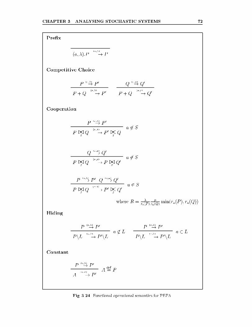
CHAPTER 3. ANALYSING STOCHASTIC SYSTEMS 72
Pre�x
(a; �):P(a;�)���! P
Competitive Choice
P(a;�)�! P 0
P +Q(a;�)���! P 0
Q(a;�)�! Q0
P +Q(a;�)���! Q0
Cooperation
P(a;�)�! P 0
P ��SQ
(a;�)���! P 0 ��SQ
a 62 S
Q(a;�)�! Q0
P ��SQ
(a;�)���! P ��SQ0
a 62 S
P(a;�)�! P 0 Q
(a;�)�! Q0
P ��SQ
(a;R)���! P 0 ��SQ0
a 2 S
where R = �ra(P )
�ra(Q)
min(ra(P ); ra(Q))
Hiding
P(a;�)�! P 0
PnL (a;�)���! P 0nLa 62 L
P(a;�)�! P 0
PnL (�;�)���! P 0nLa 2 L
Constant
P(a;�)�! P 0
A(a;�)���! P 0
Adef= P
Fig. 3.24. Functional operational semantics for PEPA.
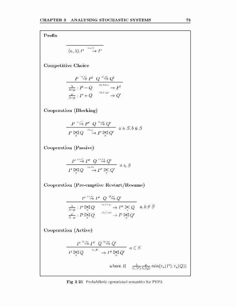
CHAPTER 3. ANALYSING STOCHASTIC SYSTEMS 73
Pre�x
(a; �):P(a;�)���! P
Competitive Choice
P(a;�)�! P 0 Q
(b;�)�! Q0
��+�
: P +Q(a;�+�)�������! P 0
��+�
: P +Q(b;�+�)�������! Q0
Cooperation (Blocking)
P(a;�)�! P 0 Q
(b;�)�! Q0
P ��SQ
(b;�)���! P ��SQ0
a 2 S; b 62 S
Cooperation (Passive)
P(a;�)�! P 0 Q
(a;>)�! Q0
P ��SQ
(a;�)���! P 0 ��SQ0
a 2 S
Cooperation (Pre-emptive Restart/Resume)
P(a;�)�! P 0 Q
(b;�)�! Q0
��+�
: P ��SQ
(a;�+�)�������! P 0 ��SQ
��+�
: P ��SQ
(b;�+�)�������! P ��SQ0
a; b 62 S
Cooperation (Active)
P(a;�)�! P 0 Q
(a;�)�! Q0
P ��SQ
(a;R)�������! P 0 ��SQ0
a 2 S
where R = �ra(P )
�ra(Q)
min(ra(P ); ra(Q))
Fig. 3.25. Probabilistic operational semantics for PEPA.
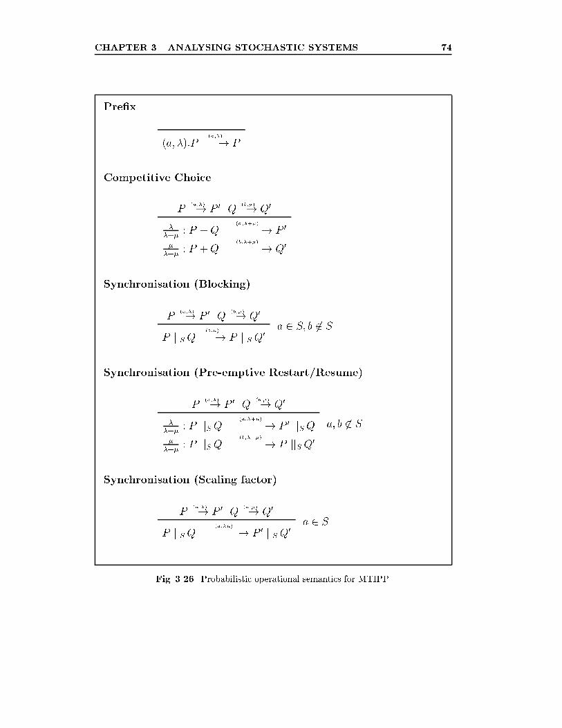
CHAPTER 3. ANALYSING STOCHASTIC SYSTEMS 74
Pre�x
(a; �):P(a;�)���! P
Competitive Choice
P(a;�)�! P 0 Q
(b;�)�! Q0
��+�
: P +Q(a;�+�)�������! P 0
��+�
: P +Q(b;�+�)�������! Q0
Synchronisation (Blocking)
P(a;�)�! P 0 Q
(b;�)�! Q0
P jjSQ(b;�)���! P jjS Q0
a 2 S; b 62 S
Synchronisation (Pre-emptive Restart/Resume)
P(a;�)�! P 0 Q
(b;�)�! Q0
��+�
: P jjSQ(a;�+�)�������! P 0 jjSQ
��+�
: P jjSQ(b;�+�)�������! P jjS Q0
a; b 62 S
Synchronisation (Scaling factor)
P(a;�)�! P 0 Q
(a;�)�! Q0
P jjSQ(a;��)�������! P 0 jjSQ0
a 2 S
Fig. 3.26. Probabilistic operational semantics for MTIPP.
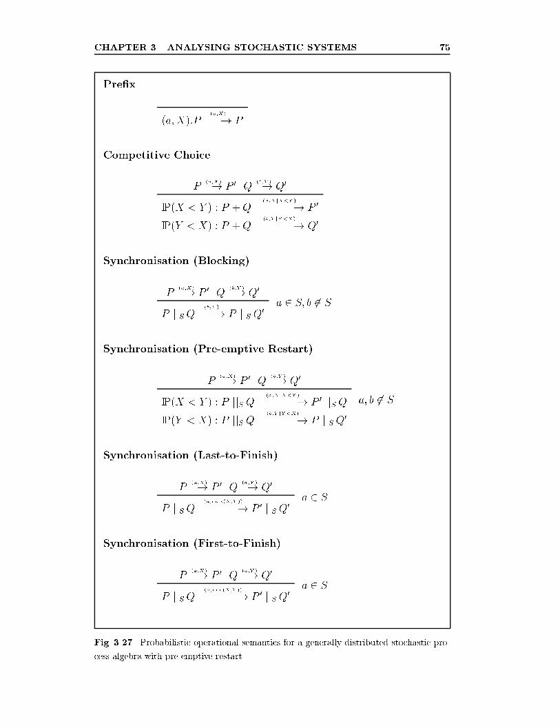
CHAPTER 3. ANALYSING STOCHASTIC SYSTEMS 75
Pre�x
(a;X):P(a;X)���! P
Competitive Choice
P(a;X)�! P 0 Q
(b;Y )�! Q0
IP(X < Y ) : P +Q(a;XjX<Y )�������! P 0
IP(Y < X) : P +Q(b;Y jY <X)�������! Q0
Synchronisation (Blocking)
P(a;X)�! P 0 Q
(b;Y )�! Q0
P jjSQ(b;Y )���! P jjS Q0
a 2 S; b 62 S
Synchronisation (Pre-emptive Restart)
P(a;X)�! P 0 Q
(b;Y )�! Q0
IP(X < Y ) : P jjS Q(a;XjX<Y )�������! P 0 jjS Q
IP(Y < X) : P jjS Q(b;Y jY <X)�������! P jjS Q0
a; b 62 S
Synchronisation (Last-to-Finish)
P(a;X)�! P 0 Q
(a;Y )�! Q0
P jjSQ(a;max(X;Y ))�������! P 0 jjSQ0
a 2 S
Synchronisation (First-to-Finish)
P(a;X)�! P 0 Q
(a;Y )�! Q0
P jjSQ(a;min(X;Y ))�������! P 0 jjSQ0
a 2 S
Fig. 3.27. Probabilistic operational semantics for a generally-distributed stochastic pro-
cess algebra with pre-emptive restart.
Chapter 4
Synchronisation in SPAs
4.1 Introduction
Markovian process algebras approximate their model of synchronising events
in order to preserve their Markovian nature. This chapter investigates syn-
chronisation models in a stochastic context. We introduce and de�ne two
distinct synchronisation models, Last-to-Finish synchronisation and First-
to-Finish synchronisation (originally presented in [15, 16]). We demonstrate
that MPAs, in trying to emulate the �rst of these models, Last-to-Finish
synchronisation, have to make a necessary approximation to the real model.
Through analysis and examples it is demonstrated how the Markovian ap-
proximation of Last-to-Finish synchronisation a�ects the accuracy of the
performance model. We compare results of four MPA models (including
MTIPP [47] and PEPA [55]) with an analytic solution to see which systems
provide better real-life synchronisations. This also allows us to suggest tac-
tics for using combinations of synchronisation models to get a more reliable
solution.
76
CHAPTER 4. SYNCHRONISATION IN SPAS 77
In focussing on this issue we accomplish half of our aim in this thesis, that
of understanding how to use current methodologies in a reliable fashion. It
is essential that the theoretical and practical advances that have been made
in MPAs are made full use of by getting a better physical understanding
of the end results. After all, it is in these purely Markovian systems that
the best opportunity exists for solving large state-space stochastic models.
This is partly as a result of MPAs having the most mature toolsets and
partly because they are a simpler paradigm than the more general stochastic
process algebras.
4.2 Synchronisation in MPAs
Purely Markovian process algebras have the following de�nition, as set out
in chapter 2:
P ::= (a; �):P P + P P jjS P P=L A (4.1)
The issue lies in the P jjSQ (or P ��SQ in PEPA notation), which repre-
sents an interaction between components of the algebra. As we will see in
sections 4.4.1 and 4.4.2 the intention is that this interaction should re ect
the progress of the slower component. Equation (4.8) shows that this quan-
tity is not exponential so some form of approximation has to be made, as
recognised in [53]:
: : : there is an assumption that the interaction, or shared action,
will have an exponentially distributed duration, in the same way
as the individual actions of the agents. This assumption is a
pragmatic one, although we will see : : : that it is not necessarily
a justi�ed one.
In section 4.3, we examine common types of synchronisation that occur in
software engineering. Section 4.4 discusses the models used by MTIPP and
CHAPTER 4. SYNCHRONISATION IN SPAS 78
PEPA and presents an analysis on how they di�er from the real-world syn-
chronisation models. Section 4.5 discusses possible synchronisation models
for MPAs which allow more accurate performance statistics to be generated.
Finally, a worked example is presented in section 4.6 which serves to com-
pare MTIPP and PEPA with each other and with the suggested models of
section 4.5.
Later stochastic process algebras have recti�ed this approximation by ex-
tending the class of distributions that can be modelled so that the slower
component in an interaction is capable of being represented precisely. This
can be done minimally by introducing immediate transitions to supplement
the Markovian transitions, as in IMC [43] and EMPA [8], for example. Other
algebras employ phase-type distributions which are also closed under this
form of synchronisation, for instance, Stochastic Causality-Based Process
Algebra [19] and El-Rayes et al's recent PEPA1ph [29].
However, many example systems have been constructed in MTIPP and es-
pecially PEPA, because of their ease-of-use [62, 11, 56, 31]. In addition,
two well developed tools have been constructed around the two algebras,
TIPPtool [46] and PEPA Workbench [33]. So this analysis can give both
extra accuracy information about existing models and con�dence to a mod-
eller wishing to use the full power of synchronisation in the two systems. It
should also be noted that many of the recent generally-distributed algebras
either do not yet have general analytic solution techniques or do not have
mature tools capable of solving the larger systems.
4.3 Real-world Synchronisation Models
In this section, we distinguish between passive synchronisation, as described
in section 4.3.1, and active synchronisations, where both or all the constituent
processes make a contribution to the activity of the synchronisation. Active
synchronisations are classi�ed in sections 4.3.2{4.3.5.
CHAPTER 4. SYNCHRONISATION IN SPAS 79
4.3.1 Client-Server
This is often referred to as passive synchronisation, where one of the pro-
cesses (the client) idles while its request is dealt with by the server process.
The client takes no active part in the activity of the synchronisation, so
the duration of the combined event is completely dependent on the server
process.
Most Markovian process algebras can deal with this type of model (certainly
PEPA and MTIPP have syntactic or numerical tricks for handling such syn-
chronisations). It should be noted that the distinction between active and
passive synchronisations is a physical one since in fact they represent limiting
cases of the synchronisation models below.
4.3.2 First-to-Finish
The First-to-Finish (FTF) synchronisation of two processes X and Y states
that the synchronisation can terminate on successful completion of either X
or Y , whichever occurs �rst. Thus FTF synchronisation follows the minimum
time duration of X and Y .
An example of this might be a distributed code-breaking e�ort between pro-
cessors, where the �rst processor to �nd the correct key brings the entire
e�ort to a close. No further processing is required as no further information
is required.
This interaction can only be used in particular circumstances. For a search-
ing problem as above, it requires that the search-space be completely divisi-
ble between processes, without any subsequent inter-process communication.
Furthermore, there must only be one solution, such that when found it is
immediately known that the remaining processes are undertaking a fruitless
search.
CHAPTER 4. SYNCHRONISATION IN SPAS 80
Stochastic Details
For general distributions X and Y , we de�ne:
FX
kFTFY
(t) = Fmin(X;Y )(t)
= IP(min(X; Y ) � t)
= 1� IP(min(X; Y ) > t)
= 1� IP(X > t)IP(Y > t)
= 1� FX(t)F Y (t) (4.2)
In the case of n synchronising processes X1; : : : ; Xn:
FX1
kFTF���
kFTFXn
(t) = 1�nYi=1
FXi(t) (4.3)
If X and Y are exponentially distributed processes with rates � and �, then
the well known result for First-to-Finish synchronisation of X and Y is gen-
erated:
fX
kFTFY
(t) = fmin(X;Y )(t) = (�+ �)e�(�+�)t (4.4)
This is signi�cant since it tells us that the FTF synchronisation of two ex-
ponential distributions is itself an exponential distribution, as shown in �g-
ure 4.1. Also, if � ! 0 in equation (4.4), equivalent to X having in�nite
mean duration, then we recover the passive client-server model, described in
section 4.3.1.
The First-to-Finish synchronisation for exponential distributions has the fol-
lowing mean and variance properties:
IE(min(X; Y )) =1
�+ �Var(min(X; Y )) =
1
(�+ �)2(4.5)
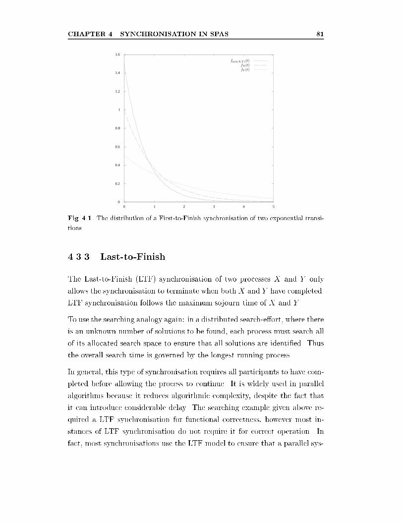
CHAPTER 4. SYNCHRONISATION IN SPAS 81
0
0.2
0.4
0.6
0.8
1
1.2
1.4
1.6
0 1 2 3 4 5
Fig. 4.1. The distribution of a First-to-Finish synchronisation of two exponential transi-
tions.
4.3.3 Last-to-Finish
The Last-to-Finish (LTF) synchronisation of two processes X and Y only
allows the synchronisation to terminate when both X and Y have completed.
LTF synchronisation follows the maximum sojourn time of X and Y .
To use the searching analogy again: in a distributed search-e�ort, where there
is an unknown number of solutions to be found, each process must search all
of its allocated search-space to ensure that all solutions are identi�ed. Thus
the overall search time is governed by the longest running process.
In general, this type of synchronisation requires all participants to have com-
pleted before allowing the process to continue. It is widely used in parallel
algorithms because it reduces algorithmic complexity, despite the fact that
it can introduce considerable delay. The searching example given above re-
quired a LTF synchronisation for functional correctness, however most in-
stances of LTF synchronisation do not require it for correct operation. In
fact, most synchronisations use the LTF model to ensure that a parallel sys-
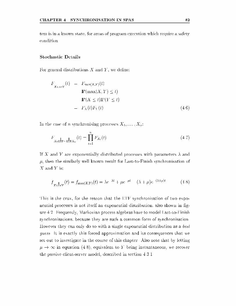
CHAPTER 4. SYNCHRONISATION IN SPAS 82
tem is in a known state, for areas of program execution which require a safety
condition.
Stochastic Details
For general distributions X and Y , we de�ne:
FX
kLTFY
(t) = Fmax(X;Y )(t)
= IP(max(X; Y ) � t)
= IP(X � t)IP(Y � t)
= FX(t)FY (t) (4.6)
In the case of n synchronising processes X1; : : : ; Xn:
FX1
kLTF���
kLTFXn
(t) =nYi=1
FXi(t) (4.7)
If X and Y are exponentially distributed processes with parameters � and
�, then the similarly well known result for Last-to-Finish synchronisation of
X and Y is:
fX
kLTFY
(t) = fmax(X;Y )(t) = �e��t + �e��t � (�+ �)e�(�+�)t (4.8)
This is the crux, for the reason that the LTF synchronisation of two expo-
nential processes is not itself an exponential distribution, also shown in �g-
ure 4.2. Frequently, Markovian process algebras have to model Last-to-Finish
synchronisations, because they are such a common form of synchronisation.
However they can only do so with a single exponential distribution as a best
guess. It is exactly this forced approximation and its consequences that we
set out to investigate in the course of this chapter. Also note that by letting
� ! 1 in equation (4.8), equivalent to Y being instantaneous, we recover
the passive client-server model, described in section 4.3.1.
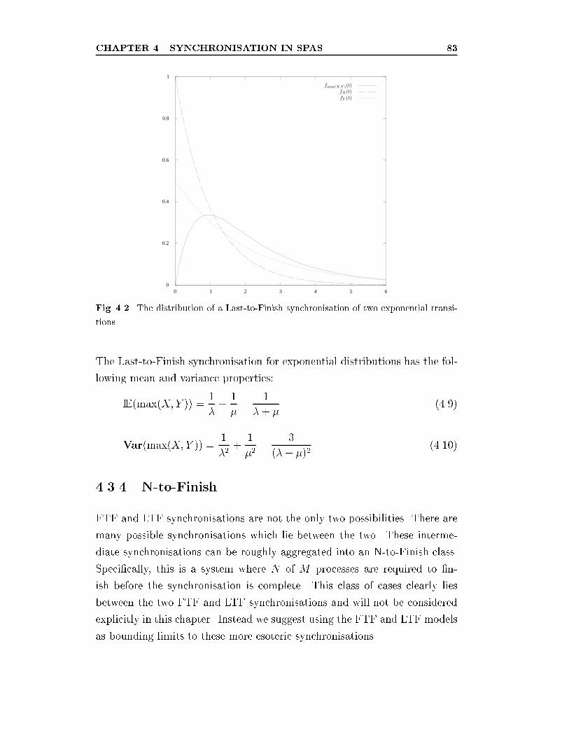
CHAPTER 4. SYNCHRONISATION IN SPAS 83
0
0.2
0.4
0.6
0.8
1
0 1 2 3 4 5 6
Fig. 4.2. The distribution of a Last-to-Finish synchronisation of two exponential transi-
tions.
The Last-to-Finish synchronisation for exponential distributions has the fol-
lowing mean and variance properties:
IE(max(X; Y )) =1
�+
1
�� 1
�+ �(4.9)
Var(max(X; Y )) =1
�2+
1
�2� 3
(�+ �)2(4.10)
4.3.4 N-to-Finish
FTF and LTF synchronisations are not the only two possibilities. There are
many possible synchronisations which lie between the two. These interme-
diate synchronisations can be roughly aggregated into an N-to-Finish class.
Speci�cally, this is a system where N of M processes are required to �n-
ish before the synchronisation is complete. This class of cases clearly lies
between the two FTF and LTF synchronisations and will not be considered
explicitly in this chapter. Instead we suggest using the FTF and LTF models
as bounding limits to these more esoteric synchronisations.
CHAPTER 4. SYNCHRONISATION IN SPAS 84
Real instances of these synchronisations do exist. In safety-critical computing
a critical function might be managed by three or more controlling programs
running in parallel. When a change of state is required, a single arbiter
program will count the votes of the controlling programs and go with the
majority decision. Because of the complexity of implementation, these forms
of synchronisation are rarely encountered.
There is no obvious two-process version of this model, but in the event that
a synchronisation with performance characteristics between that of FTF and
LTF is required, we will not discard the notion.
4.3.5 Other Models
We now argue intuitively that there are no other synchronisation models out-
side the bounds of FTF and LTF synchronisation. Consider a two-process
synchronisation which performs slower than a Last-to-Finish model. By mod-
elling the overall sojourn time of the synchronisation as a third process and
incorporating this, via another LTF synchronisation, into the original syn-
chronisation, a Last-to-Finish model can be recovered.
Similarly, consider a two-process synchronisation which performs faster than
the First-to-Finish synchronisation. By representing the faster model as a
third process and incorporating its performance into the synchronisation, a
First-to-Finish synchronisation is recovered.
Summarising our approach to synchronisation models: synchronisation is
at best First-to-Finish and at worst Last-to-Finish. Passive synchronisations
can be encompassed within this framework too: by considering them as either
a Last-to-Finish model where the client terminates instantly or a First-to-
Finish model where the client never terminates.
CHAPTER 4. SYNCHRONISATION IN SPAS 85
4.4 Comparison with MPA Synchronisations
In this section, we compare the synchronisations of two Markovian process
algebras (PEPA and MTIPP) to the real-world LTF and FTF synchronisa-
tions, outlined in section 4.3.
4.4.1 PEPA
Introduction
The PEPA synchronisation model selects the exponential distribution with
the largest mean to represent the evolution of the overall synchronisation.
Passive synchronisations have an alternative syntactic representation. In [53],
the selection of the active synchronisation style is described as follows:
The de�nition : : : is chosen to re ect the idea that the rate at
which such a joint action can occur will be limited by the rate of
the slowest participant.
Clearly, PEPA is emulating a Last-to-Finish strategy with its synchronisation
model. However, given that it is restricted to using exponential distributions,
this prevents it from using an exact LTF synchronisation, and so it has to
settle for an approximation. The details of the PEPA cooperation have been
described in detail in section 2.4.3, but in essence the synchronisation takes
the minimum rate parameter of its constituent processes.
Stochastic Details
If X is distributed with exponential parameter � and Y is distributed with
exponential parameter �, then the PEPA model (shown in �gure 4.3 against
the equivalent LTF synchronisation) has the following distribution:
Xk
PEPA Y � exp(min(�; �)) (4.11)
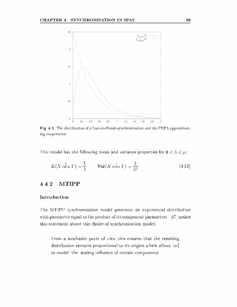
CHAPTER 4. SYNCHRONISATION IN SPAS 86
0
0.5
1
1.5
2
2.5
0 0.2 0.4 0.6 0.8 1 1.2 1.4 1.6 1.8 2
Fig. 4.3. The distribution of a Last-to-Finish synchronisation and the PEPA approximat-
ing cooperation.
This model has the following mean and variance properties for 0 < � < �:
IE(Xk
PEPA Y ) =1
�Var(X
kPEPA Y ) =
1
�2(4.12)
4.4.2 MTIPP
Introduction
The MTIPP synchronisation model generates an exponential distribution
with parameter equal to the product of its component parameters. [47] makes
this statement about this choice of synchronisation model:
From a stochastic point of view this ensures that the resulting
distribution remains proportional to its origins which allows [us]
to model [the] scaling in uence of certain components.
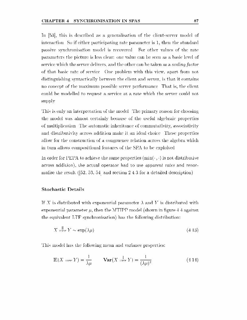
CHAPTER 4. SYNCHRONISATION IN SPAS 87
In [53], this is described as a generalisation of the client-server model of
interaction. So if either participating rate parameter is 1, then the standard
passive synchronisation model is recovered. For other values of the rate
parameters the picture is less clear: one value can be seen as a basic level of
service which the server delivers, and the other can be taken as a scaling factor
of that basic rate of service. One problem with this view, apart from not
distinguishing syntactically between the client and server, is that it contains
no concept of the maximum possible server performance. That is, the client
could be modelled to request a service at a rate which the server could not
supply.
This is only an interpretation of the model. The primary reason for choosing
the model was almost certainly because of the useful algebraic properties
of multiplication. The automatic inheritance of commutativity, associativity
and distributivity across addition make it an ideal choice. These properties
allow for the construction of a congruence relation across the algebra which
in turn allows compositional features of the SPA to be exploited.
In order for PEPA to achieve the same properties (min(� ; �) is not distributiveacross addition), the actual operator had to use apparent rates and renor-
malise the result ([52, 53, 54] and section 2.4.3 for a detailed description).
Stochastic Details
If X is distributed with exponential parameter � and Y is distributed with
exponential parameter �, then the MTIPP model (shown in �gure 4.4 against
the equivalent LTF synchronisation) has the following distribution:
Xk
TIPP Y � exp(��) (4.13)
This model has the following mean and variance properties:
IE(Xk
TIPP Y ) =1
��Var(X
kTIPP Y ) =
1
(��)2(4.14)
CHAPTER 4. SYNCHRONISATION IN SPAS 88
0
1
2
3
4
5
6
7
8
9
0 0.2 0.4 0.6 0.8 1 1.2 1.4 1.6 1.8 2
Fig. 4.4. The distribution of a Last-to-Finish synchronisation and the MTIPP approxi-
mating synchronisation.
4.4.3 Comparing MTIPP and PEPA Synchronisations
In the following sections, we summarise the stochastic properties of MTIPP
and PEPA in comparison with the standard FTF and LTF models (details
in the annex section 4.A). It is useful to compare expected synchronisa-
tion times, in each case, as this gives us an indication of how the mean
performance predictions of the MPA models will di�er from the real-world
behaviour.
PEPA
For PEPA, the synchronisation model turns out to be static relative to the
LTF and FTF models. From section 4.A, for all 0 < � < �, we have:
IE(Xk
FTF Y ) < IE(Xk
PEPA Y ) < IE(Xk
LTF Y ) (4.15)
Clearly PEPA is modelling a valid synchronisation and one closer to LTF
CHAPTER 4. SYNCHRONISATION IN SPAS 89
than FTF (as is obvious from its choice of min(� ; �) operator). However, thefact that it underestimates the synchronisation mean will have a large e�ect
on the steady-state solution of the CTMC. By underestimating the mean or
overestimating the rate, PEPA will tend to overestimate the performance or
capacity of a system. This is further borne out by the worked example in
section 4.6.
MTIPP
For MTIPP, the synchronisation is not at all static compared to the LTF and
FTF models. Summarising the detailed results in section 4.A:
IE(Xk
TIPP Y ) < IE(Xk
FTF Y ) for 0 < � < � i�:
1 +�
�< � <1 (4.16)
IE(Xk
FTF Y ) < IE(Xk
TIPP Y ) < IE(Xk
LTF Y ) for 0 < � < � i� either:8>><>>:
1 < � < 2 and �� 1 < ��< 1
23< � < 1
0 < � < 23
and 0 < ��< 1
2
h�1 +
q1+3�1��
i (4.17)
IE(Xk
LTF Y ) < IE(Xk
TIPP Y ) for 0 < � < � i�:
0 < � <2
3and
1
2
"�1 +
r1 + 3�
1� �
#<�
�< 1 (4.18)
Since MTIPP's synchronisation model varies over the whole spectrum of
other models, it is di�cult to generalise its e�ect on performance modelling.
However, it is clear that it would be possible to construct a system which
either underestimated or overestimated the performance across a particular
synchronisation, according to the choice of parameters. To maintain the cri-
terion discussed in section 4.3.5, MTIPP should not have to stray outside
CHAPTER 4. SYNCHRONISATION IN SPAS 90
the bounds provided by FTF and LTF synchronisation. Given this require-
ment, the allowable parameter space for MTIPP needs to be restricted by
the ranges speci�ed in equation (4.17). MTIPP's relative performance char-
acteristics are compared with the other models in the worked example in
section 4.6.
4.5 Alternative Synchronisation Strategies
The aim of this section is to suggest methods which accurately approximate a
Last-to-Finish model. In one case, this involves maintaining the exponential
distribution and suggesting an alternative synchronisation rate, and in the
other two instances we suggest methods which use and augment the MTIPP
and PEPA models. By following these di�erent models through to the steady-
state solution stage in section 4.6, we can then make qualitative statements
about the errors that the MPA approximations introduce.
4.5.1 Mean-preserving Synchronisation
The result of solving the CTMC for an MPA system is the steady-state
distribution for that system, that is, a description of the long-run average
behaviour.
One possible solution would be to design an exponential synchronisation with
the same mean as the LTF synchronisation. In this way, the correct average
behaviour for each synchronisation is propagated into the CTMC. So we need
to �nd the exponential distribution with mean (from equation (4.9)):
1
�+
1
�� 1
�+ �(4.19)
That is, we require a random variable Z � exp( ) such that:
1
=
1
�+
1
�� 1
�+ �(4.20)
CHAPTER 4. SYNCHRONISATION IN SPAS 91
Thus:
=��(�+ �)
(�+ �)2 � �� (4.21)
In the notation of [53], we would write:
R = � � =��(�+ �)
(�+ �)2 � �� (4.22)
It should be noted that this operator is neither associative nor distributive
over addition, so it is not possible to construct a congruence and make use
of system decomposition in solving the model. Its relative performance char-
acteristics are compared with the other models in the worked example in
section 4.6.
4.5.2 Using PEPA to Bound the LTF Synchronisation
Unlike MTIPP, PEPA maintains the same mean characteristics in its syn-
chronisation relative to the LTF and FTF models, for all parameter values
(annex 4.A). That is, from equation (4.15), for all 0 < � < �:
IE(Xk
FTF Y ) < IE(Xk
PEPA Y ) < IE(Xk
LTF Y )
A possible approach for system design would be to design a dual synchroni-
sation model to that of PEPA, whose mean is always greater than that of the
LTF model. In doing this, we aim to try and bound the performance of the
real synchronisation model with PEPA above and what we now call PEPA*
below. So for all 0 < � < �, we require:
IE(Xk
FTF Y ) < IE(Xk
PEPA Y ) < IE(Xk
LTF Y ) < IE(Xk
PEPA* Y ) (4.23)
If we de�ne PEPA* to have synchronisation1:
Xk
PEPA* Y � exp
���
�+ �
�(4.24)
1The reason that we have assigned the new synchronisation the label PEPA*, is that,
coincidentally, it used to be the old synchronisation model for PEPA [53].
CHAPTER 4. SYNCHRONISATION IN SPAS 92
Now:
IE(Xk
PEPA* Y ) =1
�+
1
�(4.25)
and since for all �; � > 0:
1
�+
1
�� 1
�+ �<
1
�+
1
�(4.26)
) IE(Xk
LTF Y ) < IE(Xk
PEPA* Y ) (4.27)
So PEPA* matches the criterion. Now, in order to obtain bounds for the
LTF synchronisation we can derive solutions with the PEPA model and with
the PEPA* model.
It should be noted that, as stated, the PEPA* operator is not distributive
across addition (it is associative). It is possible that a similar �nesse to the
one used on the PEPA operator involving apparent rates can be performed
on this operator to make it distributive, however we are not aware of one.
4.5.3 Restricted MTIPP Synchronisation
Unlike PEPA, MTIPP does not have a stable synchronisation model; by which
we mean that, for certain parameter values, it can have a mean less than or
greater than the means of the LTF or FTF synchronisation (section 4.4.3).
If, therefore, we require MTIPP to model the FTF or LTF synchronisation
by forcing the mean of the MTIPP synchronisation to equal that of the real-
world model, what restrictions does this place on MTIPP?
Thm. 2. IE(Xk
TIPP Y ) = IE(Xk
FTF Y ) i�, for 0 < � < �, both:
1 < � < 2 and � =�
�� 1such that 1 > � > 2 (4.28)
CHAPTER 4. SYNCHRONISATION IN SPAS 93
Proof. Assuming 0 < � < � and thus 0 < �=� < 1:
IE(Xk
TIPP Y ) = IE(Xk
FTF Y ) (4.29)
, 1
��=
1
�+ �(4.30)
,(� = �
��1
1 < � < 2(4.31)
Thm. 3. IE(Xk
TIPP Y ) = IE(Xk
LTF Y ) i�, for 0 < � < �, both:
0 < � <2
3and � =
1
2
h(1� �) +
p(1� �)(1 + 3�)
isuch that 1 > � >
2
3(4.32)
Proof. Assuming 0 < � < � and thus 0 < �=� < 1:
IE(Xk
TIPP Y ) = IE(Xk
LTF Y ) (4.33)
, 1
�+
1
�� 1
�+ �=
1
��(4.34)
, �
�=
1
2
"�1�
r1 +
4�
1� �
#(4.35)
,(� = 1
2
h(1� �) +p(1� �)(1 + 3�)
i0 < � < 2
3
(4.36)
So now for these speci�c ranges of � (the smaller rate) the value of � is
�xed and a synchronisation can take place for which the mean behaviour
is identical to that of LTF or FTF synchronisation. This is not a general
panacea however, since there is no guarantee that the synchronisations in a
model will have the appropriate rates. Indeed, it is easy to construct an LTF
synchronisation of two legitimate LTF synchronisations which cannot then
be modelled in MTIPP.
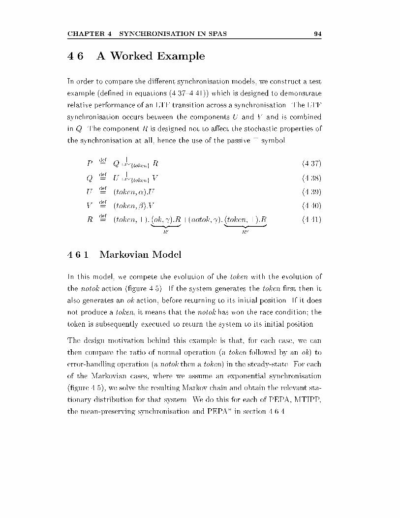
CHAPTER 4. SYNCHRONISATION IN SPAS 94
4.6 A Worked Example
In order to compare the di�erent synchronisation models, we construct a test
example (de�ned in equations (4.37{4.41)) which is designed to demonstrate
relative performance of an LTF transition across a synchronisation. The LTF
synchronisation occurs between the components U and V and is combined
in Q. The component R is designed not to a�ect the stochastic properties of
the synchronisation at all, hence the use of the passive > symbol.
Pdef= Q
kLTFftokeng R (4.37)
Qdef= U
kLTFftokeng V (4.38)
Udef= (token; �):U (4.39)
Vdef= (token; �):V (4.40)
Rdef= (token;>): (ok; ):R| {z }
R0
+(notok; ): (token;>):R| {z }R00
(4.41)
4.6.1 Markovian Model
In this model, we compete the evolution of the token with the evolution of
the notok action (�gure 4.5). If the system generates the token �rst then it
also generates an ok action, before returning to its initial position. If it does
not produce a token, it means that the notok has won the race condition; the
token is subsequently executed to return the system to its initial position.
The design motivation behind this example is that, for each case, we can
then compare the ratio of normal operation (a token followed by an ok) to
error-handling operation (a notok then a token) in the steady-state. For each
of the Markovian cases, where we assume an exponential synchronisation
(�gure 4.5), we solve the resulting Markov chain and obtain the relevant sta-
tionary distribution for that system. We do this for each of PEPA, MTIPP,
the mean-preserving synchronisation and PEPA* in section 4.6.4.
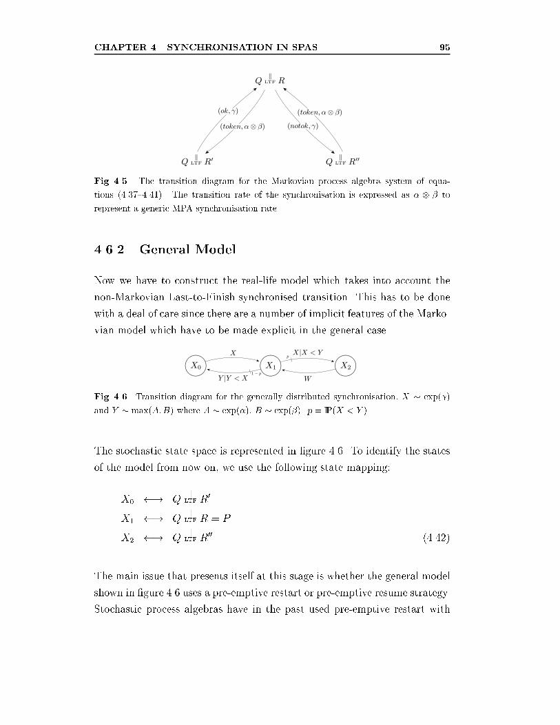
CHAPTER 4. SYNCHRONISATION IN SPAS 95
Fig. 4.5. The transition diagram for the Markovian process algebra system of equa-
tions (4.37{4.41). The transition rate of the synchronisation is expressed as � � to
represent a generic MPA synchronisation rate.
4.6.2 General Model
Now we have to construct the real-life model which takes into account the
non-Markovian Last-to-Finish synchronised transition. This has to be done
with a deal of care since there are a number of implicit features of the Marko-
vian model which have to be made explicit in the general case.
Fig. 4.6. Transition diagram for the generally distributed synchronisation, X � exp( )
and Y � max(A;B) where A � exp(�), B � exp(�). p = IP(X < Y ).
The stochastic state space is represented in �gure 4.6. To identify the states
of the model from now on, we use the following state mapping:
X0 ! Qk
LTF R0
X1 ! Qk
LTF R = P
X2 ! Qk
LTF R00 (4.42)
The main issue that presents itself at this stage is whether the general model
shown in �gure 4.6 uses a pre-emptive restart or pre-emptive resume strategy.
Stochastic process algebras have in the past used pre-emptive restart with
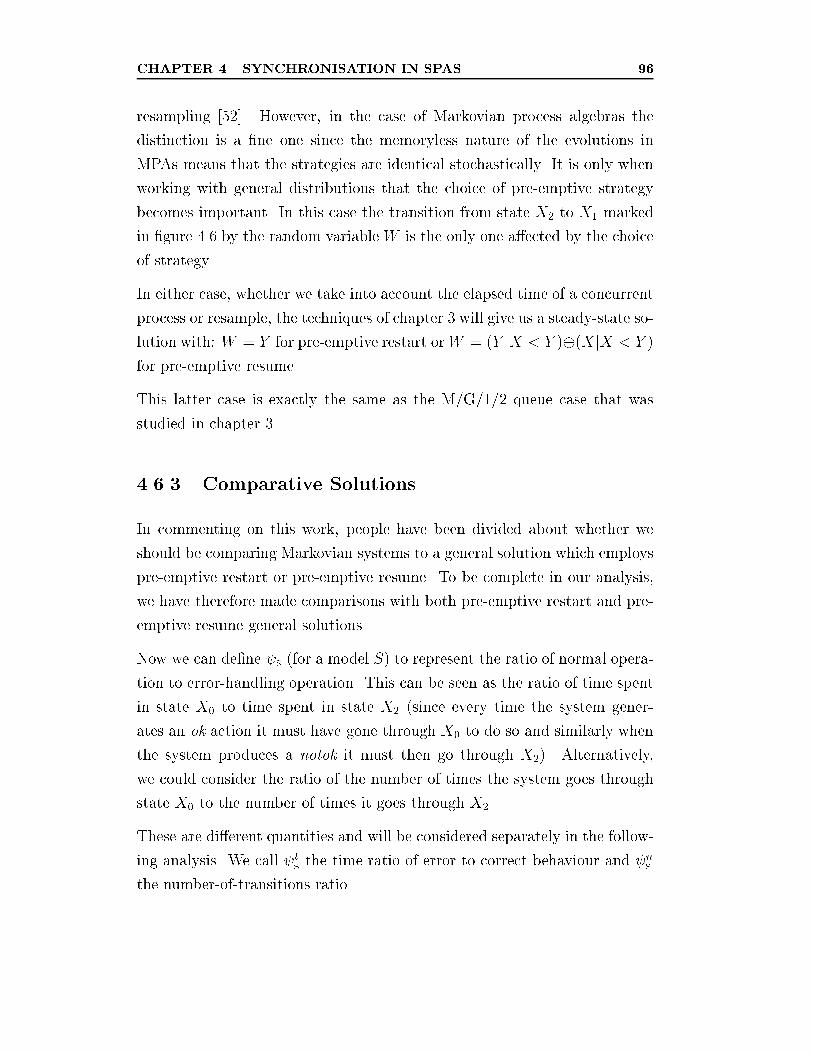
CHAPTER 4. SYNCHRONISATION IN SPAS 96
resampling [52]. However, in the case of Markovian process algebras the
distinction is a �ne one since the memoryless nature of the evolutions in
MPAs means that the strategies are identical stochastically. It is only when
working with general distributions that the choice of pre-emptive strategy
becomes important. In this case the transition from state X2 to X1 marked
in �gure 4.6 by the random variableW is the only one a�ected by the choice
of strategy.
In either case, whether we take into account the elapsed time of a concurrent
process or resample, the techniques of chapter 3 will give us a steady-state so-
lution with: W = Y for pre-emptive restart orW = (Y jX < Y )(XjX < Y )
for pre-emptive resume.
This latter case is exactly the same as the M/G/1/2 queue case that was
studied in chapter 3.
4.6.3 Comparative Solutions
In commenting on this work, people have been divided about whether we
should be comparing Markovian systems to a general solution which employs
pre-emptive restart or pre-emptive resume. To be complete in our analysis,
we have therefore made comparisons with both pre-emptive restart and pre-
emptive resume general solutions.
Now we can de�ne S (for a model S) to represent the ratio of normal opera-
tion to error-handling operation. This can be seen as the ratio of time spent
in state X0 to time spent in state X2 (since every time the system gener-
ates an ok action it must have gone through X0 to do so and similarly when
the system produces a notok it must then go through X2). Alternatively,
we could consider the ratio of the number of times the system goes through
state X0 to the number of times it goes through X2.
These are di�erent quantities and will be considered separately in the follow-
ing analysis. We call tSthe time ratio of error to correct behaviour and n
S
the number-of-transitions ratio.
CHAPTER 4. SYNCHRONISATION IN SPAS 97
tS=
�(X0)
�(X2)(4.43)
nS=
�(X0)
IE(X)
��(X2)
IE(W )(4.44)
whereW , from �gure 4.6, represents the random variable which is a�ected by
the choice of pre-emptive strategy. This gives us four general model ratios:
nRESTART
, nRESUME
, tRESTART
and tRESUME
.
Now for each of the above approximate Markovian models, we have a proper
yardstick by which to judge their accuracy in Last-to-Finish synchronisation.
The general model is solved in section 4.6.5 and the comparative results are
presented in section 4.6.6.
4.6.4 Markovian Solution
We can solve this system generally for all MPAs of the MTIPP and PEPA
variety. Figure 4.5 shows the transition diagram for the general Markovian
model. By setting � = � �, the synchronisation operator, we obtain the
Markov chain generator matrix, G:
G =
0B@ � 0
� �(� + )
0 � ��
1CA (4.45)
Using Gaussian elimination, we �nd the stationary probability vector �(Xi)
such that �G = 0 andP
i�(Xi) = 1. We obtain:
�(X0) =�2
2 + � + �2(4.46)
�(X1) =�
2 + � + �2(4.47)
�(X2) = 2
2 + � + �2(4.48)
CHAPTER 4. SYNCHRONISATION IN SPAS 98
Now from section 4.6.3:
tS=
�(X0)
�(X2)=
��
�2
(4.49)
Since in the Markovian case, W � exp(�):
nS=
�(X0)
IE(X)
��(X2)
IE(W )=�
=p tS
(4.50)
As mentioned before, we do not have to treat pre-emptive restart and pre-
emptive resume di�erently for Markovian systems since they are observation-
ally the same.
PEPA
For � = min(�; �) = � for 0 < � < � WLOG, equations (4.49) and (4.50)
give:
tPEPA
=
��
�2
nPEPA
=�
(4.51)
MTIPP
For � = ��, equations (4.49) and (4.50) give:
tTIPP
=
���
�2
nTIPP
=��
(4.52)
Mean-preserving Synchronisation
For:
� =��(�+ �)
(� + �)2 � �� (4.53)
Equations (4.49) and (4.50) give:
tMEAN
=
���(�+ �)
(�2 + �� + �2)
�2
nMEAN
=��(�+ �)
(�2 + �� + �2)(4.54)
CHAPTER 4. SYNCHRONISATION IN SPAS 99
PEPA*
For:
� =��
� + �(4.55)
Equations (4.49) and (4.50) give:
tPEPA*
=
���
(� + �)
�2
nPEPA*
=��
(� + �)(4.56)
4.6.5 Analytic Solution
General Pre-emptive Resume Model
In the pre-emptive resume case, we observe that our example system has
an underlying stochastic transition system of an M/G/1/2 queueing system.
Thus using standard queueing techniques from [26] and [66] or our aggrega-
tion technique from chapter 3, we can obtain the precise analytical solution
for the steady-state distribution. In the queueing case, we choose the gen-
eral service time distribution to be the maximum of the two exponential
distributions with parameters � and �, as in equation (4.8).
We obtain:
�(X0) =�
�+ �(4.57)
�(X1) =1� ��+ �
(4.58)
�(X2) = 1� 1
�+ �(4.59)
where:
� =1
�+
1
�� 1
� + �(4.60)
� =�
�+ +
�
� + � � + �
� + � + (4.61)
CHAPTER 4. SYNCHRONISATION IN SPAS 100
Now, as before we can calculate tSand n
Susing equations (4.43) and (4.44):
tRESUME
=�(X0)
�(X2)=
�
�+ �� 1(4.62)
nRESUME
=�(X0)
IE(X)
��(X2)
IE(W )=��(�+ � + 2 )
�(4.63)
where � = (� + � + )2 � ��.
General Pre-emptive Restart Model
Using the stochastic aggregation technique from chapter 3 with the appro-
priate value of W (�gure 4.6) for pre-emptive restart, we obtain:
�(X0) =�2�2(�+ �)(� + � + 2 )
�(4.64)
�(X1) =�� (�+ �)�
�(4.65)
�(X2) = 2(�2 + �� + �2)�
�(4.66)
where � = (� + � + )2 � �� as before, and:
� = �2�2(� + �)(�+ � + 2 ) + �� (�+ �)� + 2(�2 + �� + �2)�
= (�2 + �� + �2) 4 + (� + �)(2�2 + 3�� + 2�2) 3
+ (�4 + 4�3� + 7�2�2 + 4��3 + �4) 2
+ ��(�+ �)(�2 + 3�� + �2) + �2�2(� + �)2 (4.67)
Now, as before we can calculate tSand n
Susing equations (4.43) and (4.44):
tRESTART
=�(X0)
�(X2)=�2�2(� + �)(�+ � + 2 )
2(�2 + �� + �2)�(4.68)
nRESTART
=�(X0)
IE(X)
��(X2)
IE(W )=��(�+ � + 2 )
�(4.69)
CHAPTER 4. SYNCHRONISATION IN SPAS 101
This coincidence, the fact that nRESTART
= nRESUME
, is explained by con-
sidering an alternative analysis of the physical meaning of the number-of-
transitions ratio, de�ned in section 4.6.3. The quantity nSreturns the ratio
of the number of times the system passes down one branch (X1 to X0) as
opposed to going down the other (X1 to X2). This can be more simply ex-
pressed as the ratio of the probability that the system goes one way to the
probability that it goes the other. Since the probabilities at this point are
identical for each pre-emptive strategy, the quantities nRESTART
and nRESUME
will also be identical.
4.6.6 Model Comparisons
General Results
We are looking for general statements that can be made comparing S with
tRESTART
, tRESUME
and2 nRESTART
. The �rst result to note is:
tRESTART
< tRESUME
(4.70)
This is because the restart strategy means that longer is spent in the error
branch of the system and therefore the overall ratio of time spent doing
normal operation will be lower. What does this mean when we come to
make comparisons with S for other models? It gives us a larger margin
within which to aim, when judging whether a Markovian model produces
a good approximation to reality. (Figures 4.7{4.10 show various graphical
comparisons). Given that it is a point of debate whether the Markovian
models are trying to reproduce pre-emptive restart or pre-emptive resume
strategies, it seems reasonable to compare the Markovian systems with both.
Similarly, the following properties are true of our various metrics, for all �,
�, :
tRESTART
< tMEAN
tRESTART
< tPEPA
tRESUME
< tPEPA
(4.71)
2Since n
RESTART= n
RESUME, we only consider n
RESTARTfrom now on when discussing
the relative number metric.
CHAPTER 4. SYNCHRONISATION IN SPAS 102
Also:
nRESTART
< nMEAN
nRESTART
< nPEPA
(4.72)
The PEPA results are consistent with predictions from the expectation re-
sults of section 4.4.3. It would seem intuitive to infer that other examples
which simulate Last-to-Finish synchronisation will also have similar qualita-
tive results.
As we hoped, our mean-preserving synchronisation lies between PEPA and
PEPA*, that is for all �, �, :
tPEPA*
< tMEAN
< tPEPA
(4.73)
and:
nPEPA*
< nMEAN
< nPEPA
(4.74)
However, unfortunately, it is not true to say that our suggested bounding
model PEPA* always underestimates performance, since neither tPEPA*
nor
nPEPA*
is consistently less than any of the analytically obtained ratios. In
fact, it turns out that no Markovian synchronisation model can always un-
derestimate any of tRESTART
, tRESUME
or nRESTART
. This statement has more
general consequences and leads to:
Thm. 4. There does not exist any Markovian synchronisation which can
consistently underestimate (or equal) the correct performance model of an
LTF synchronisation for all possible systems.
Proof. We use the example de�ned in this section as a counterexample
to the hypothesis: \There exists a Markovian synchronisation which can
consistently underestimate (or equal) the correct performance model of an
LTF synchronisation for all possible systems". To achieve this, we have to
demonstrate a contradiction for all three of the pre-emptive restart timed,
pre-emptive resume timed and pre-emptive restart number-of-transitions ra-
tios. In fact, the proofs for each of tRESUME
and nRESTART
are identical in
CHAPTER 4. SYNCHRONISATION IN SPAS 103
structure and method to the one below, where we consider the pre-emptive
restart timed ratio, tRESTART
.
For any MPA model S, equation (4.49) gives:
tS=
��s(�; �)
�2
(4.75)
From equation (4.68), we can derive:
tRESTART
=
���
�2(� + �)(�+ � + 2 )
R(�; �; )(4.76)
where:
R(�; �; ) = (�2 + �� + �2)[ 2 + 2(� + �) + (�2 + �� + �2)] (4.77)
We require tS< t
RESTARTfor all �, �, . So WLOG by setting �s(�; �) =
��1s (�; �), we get equation (4.78).
(��)2(� + �)�2s(�; �)(�+ � + 2 )| {z }(�)
�R(�; �; ) > 0 (4.78)
However, (�) can only beO( ), independent of the choice of �s(�; �), whereas
R(�; �; ) is O( 2). Thus LHS of equation (4.78) < 0 for some �; �; .
So, our worked example acts as a counterexample and we have shown quite
a powerful result. It shows that no Markovian process algebra can always
underestimate the performance of a system. We have shown this for both
pre-emptive restart and pre-emptive resume and two di�erent de�nitions of
performance.
This result is almost certainly a consequence of the original Markovian as-
sumption of all MPAs.
However, all is not lost for PEPA*. Examination of the algebra indicates
that, for many parameter values, PEPA* will still underestimate the correct
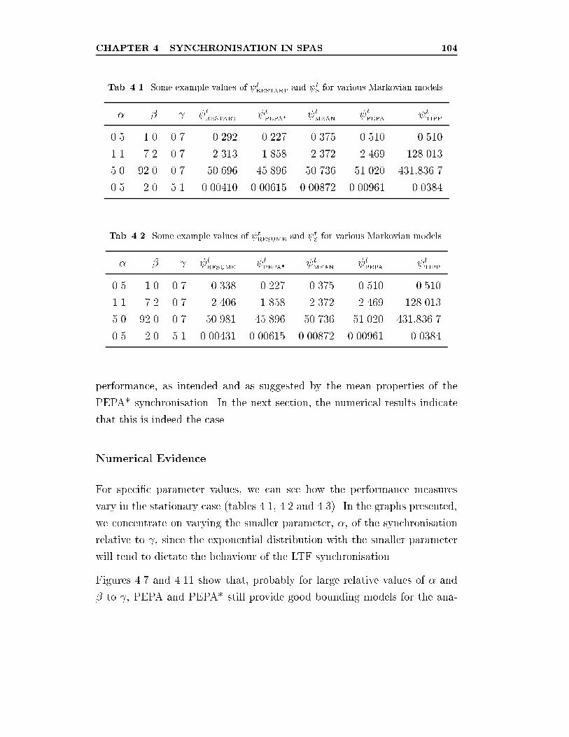
CHAPTER 4. SYNCHRONISATION IN SPAS 104
Tab. 4.1. Some example values of t
RESTARTand t
Sfor various Markovian models.
� � tRESTART
tPEPA*
tMEAN
tPEPA
tTIPP
0.5 1.0 0.7 0.292 0.227 0.375 0.510 0.510
1.1 7.2 0.7 2.313 1.858 2.372 2.469 128.013
5.0 92.0 0.7 50.696 45.896 50.736 51.020 431,836.7
0.5 2.0 5.1 0.00410 0.00615 0.00872 0.00961 0.0384
Tab. 4.2. Some example values of t
RESUMEand t
Sfor various Markovian models.
� � tRESUME
tPEPA*
tMEAN
tPEPA
tTIPP
0.5 1.0 0.7 0.338 0.227 0.375 0.510 0.510
1.1 7.2 0.7 2.406 1.858 2.372 2.469 128.013
5.0 92.0 0.7 50.981 45.896 50.736 51.020 431,836.7
0.5 2.0 5.1 0.00431 0.00615 0.00872 0.00961 0.0384
performance, as intended and as suggested by the mean properties of the
PEPA* synchronisation. In the next section, the numerical results indicate
that this is indeed the case.
Numerical Evidence
For speci�c parameter values, we can see how the performance measures
vary in the stationary case (tables 4.1, 4.2 and 4.3). In the graphs presented,
we concentrate on varying the smaller parameter, �, of the synchronisation
relative to , since the exponential distribution with the smaller parameter
will tend to dictate the behaviour of the LTF synchronisation.
Figures 4.7 and 4.11 show that, probably for large relative values of � and
� to , PEPA and PEPA* still provide good bounding models for the ana-
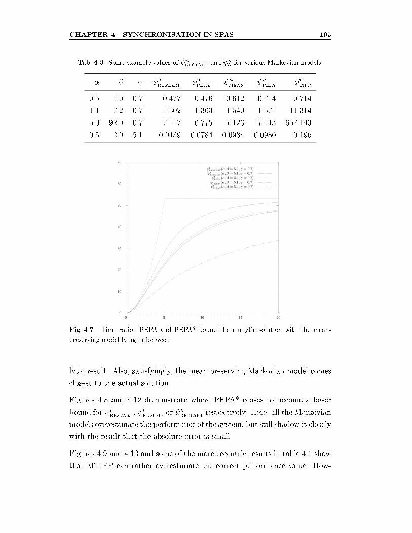
CHAPTER 4. SYNCHRONISATION IN SPAS 105
Tab. 4.3. Some example values of n
RESTARTand n
Sfor various Markovian models.
� � nRESTART
nPEPA*
nMEAN
nPEPA
nTIPP
0.5 1.0 0.7 0.477 0.476 0.612 0.714 0.714
1.1 7.2 0.7 1.502 1.363 1.540 1.571 11.314
5.0 92.0 0.7 7.117 6.775 7.123 7.143 657.143
0.5 2.0 5.1 0.0439 0.0784 0.0934 0.0980 0.196
0
10
20
30
40
50
60
70
0 5 10 15 20
Fig. 4.7. Time ratio: PEPA and PEPA* bound the analytic solution with the mean-
preserving model lying in between.
lytic result. Also, satisfyingly, the mean-preserving Markovian model comes
closest to the actual solution.
Figures 4.8 and 4.12 demonstrate where PEPA* ceases to become a lower
bound for tRESTART
, tRESUME
or nRESTART
respectively. Here, all the Markovian
models overestimate the performance of the system, but still shadow it closely
with the result that the absolute error is small.
Figures 4.9 and 4.13 and some of the more eccentric results in table 4.1 show
that MTIPP can rather overestimate the correct performance value. How-
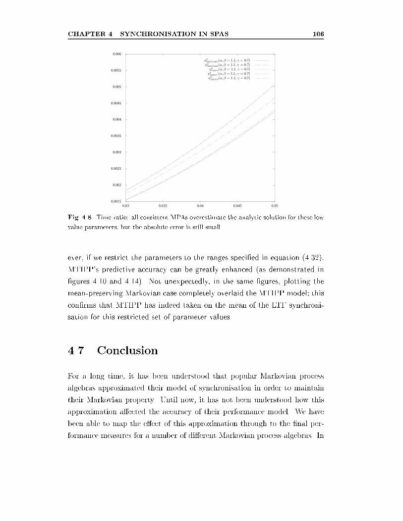
CHAPTER 4. SYNCHRONISATION IN SPAS 106
0.0015
0.002
0.0025
0.003
0.0035
0.004
0.0045
0.005
0.0055
0.006
0.03 0.035 0.04 0.045 0.05
Fig. 4.8. Time ratio: all consistent MPAs overestimate the analytic solution for these low
value parameters, but the absolute error is still small.
ever, if we restrict the parameters to the ranges speci�ed in equation (4.32),
MTIPP's predictive accuracy can be greatly enhanced (as demonstrated in
�gures 4.10 and 4.14). Not unexpectedly, in the same �gures, plotting the
mean-preserving Markovian case completely overlaid the MTIPP model; this
con�rms that MTIPP has indeed taken on the mean of the LTF synchroni-
sation for this restricted set of parameter values.
4.7 Conclusion
For a long time, it has been understood that popular Markovian process
algebras approximated their model of synchronisation in order to maintain
their Markovian property. Until now, it has not been understood how this
approximation a�ected the accuracy of their performance model. We have
been able to map the e�ect of this approximation through to the �nal per-
formance measures for a number of di�erent Markovian process algebras. In
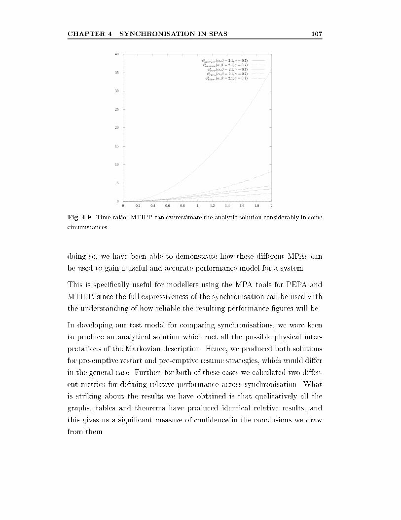
CHAPTER 4. SYNCHRONISATION IN SPAS 107
0
5
10
15
20
25
30
35
40
0 0.2 0.4 0.6 0.8 1 1.2 1.4 1.6 1.8 2
Fig. 4.9. Time ratio: MTIPP can overestimate the analytic solution considerably in some
circumstances.
doing so, we have been able to demonstrate how these di�erent MPAs can
be used to gain a useful and accurate performance model for a system.
This is speci�cally useful for modellers using the MPA tools for PEPA and
MTIPP, since the full expressiveness of the synchronisation can be used with
the understanding of how reliable the resulting performance �gures will be.
In developing our test model for comparing synchronisations, we were keen
to produce an analytical solution which met all the possible physical inter-
pretations of the Markovian description. Hence, we produced both solutions
for pre-emptive restart and pre-emptive resume strategies, which would di�er
in the general case. Further, for both of these cases we calculated two di�er-
ent metrics for de�ning relative performance across synchronisation. What
is striking about the results we have obtained is that qualitatively all the
graphs, tables and theorems have produced identical relative results, and
this gives us a signi�cant measure of con�dence in the conclusions we draw
from them.

CHAPTER 4. SYNCHRONISATION IN SPAS 108
0
0.2
0.4
0.6
0.8
1
1.2
0 0.2 0.4 0.6 0.8 1
Fig. 4.10. Time ratio: if the parameter values are restricted to the ranges in equa-
tion (4.32), then MTIPP can simulate LTF synchronisation with reasonable accuracy.
4.7.1 Summary
In this chapter, we have developed real-world synchronisation models and
shown how they can be described in the �eld of Stochastic Process Algebras.
We �nd two forms of general synchronisation model which can usefully act as
bounds to other synchronisation models, namely Last-to-Finish (LTF) and
First-to-Finish (FTF) synchronisation.
Since most of the current work on SPAs involves specialising to the Markovian
case, we have examined in detail how these general models of synchronisation
compare to the Markovian models used in MTIPP and PEPA. It is interesting
to note that most stochastic process algebras implement a form of Last-
to-Finish synchronisation; only Stark's Probabilistic I/O Automata [92] (a
Markovian process algebra), to our knowledge, uses a First-to-Finish strategy.
From what we have seen, no stochastic process algebra implements multiple
synchronisation strategies, which would clearly be appropriate for su�cient
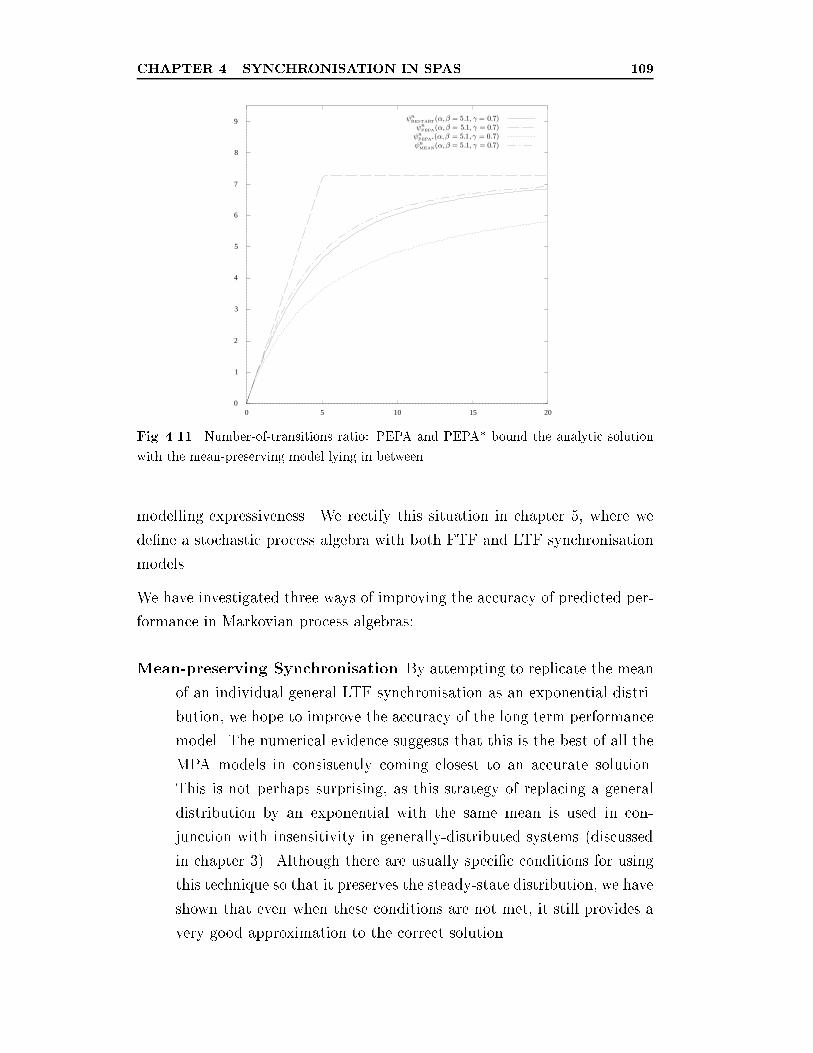
CHAPTER 4. SYNCHRONISATION IN SPAS 109
0
1
2
3
4
5
6
7
8
9
0 5 10 15 20
Fig. 4.11. Number-of-transitions ratio: PEPA and PEPA* bound the analytic solution
with the mean-preserving model lying in between.
modelling expressiveness. We rectify this situation in chapter 5, where we
de�ne a stochastic process algebra with both FTF and LTF synchronisation
models.
We have investigated three ways of improving the accuracy of predicted per-
formance in Markovian process algebras:
Mean-preserving Synchronisation By attempting to replicate the mean
of an individual general LTF synchronisation as an exponential distri-
bution, we hope to improve the accuracy of the long term performance
model. The numerical evidence suggests that this is the best of all the
MPA models in consistently coming closest to an accurate solution.
This is not perhaps surprising, as this strategy of replacing a general
distribution by an exponential with the same mean is used in con-
junction with insensitivity in generally-distributed systems (discussed
in chapter 3). Although there are usually speci�c conditions for using
this technique so that it preserves the steady-state distribution, we have
shown that even when these conditions are not met, it still provides a
very good approximation to the correct solution.
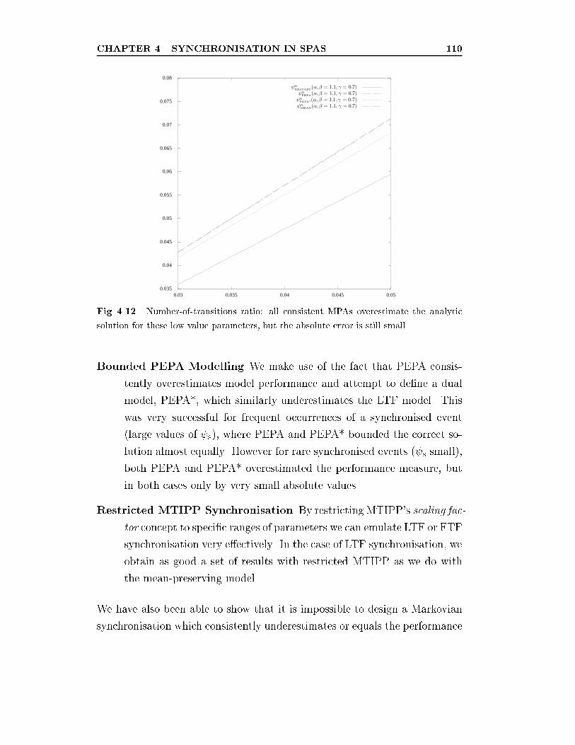
CHAPTER 4. SYNCHRONISATION IN SPAS 110
0.035
0.04
0.045
0.05
0.055
0.06
0.065
0.07
0.075
0.08
0.03 0.035 0.04 0.045 0.05
Fig. 4.12. Number-of-transitions ratio: all consistent MPAs overestimate the analytic
solution for these low value parameters, but the absolute error is still small.
Bounded PEPA Modelling We make use of the fact that PEPA consis-
tently overestimates model performance and attempt to de�ne a dual
model, PEPA*, which similarly underestimates the LTF model. This
was very successful for frequent occurrences of a synchronised event
(large values of S), where PEPA and PEPA* bounded the correct so-
lution almost equally. However for rare synchronised events ( S small),
both PEPA and PEPA* overestimated the performance measure, but
in both cases only by very small absolute values.
Restricted MTIPP Synchronisation By restricting MTIPP's scaling fac-
tor concept to speci�c ranges of parameters we can emulate LTF or FTF
synchronisation very e�ectively. In the case of LTF synchronisation, we
obtain as good a set of results with restricted MTIPP as we do with
the mean-preserving model.
We have also been able to show that it is impossible to design a Markovian
synchronisation which consistently underestimates or equals the performance
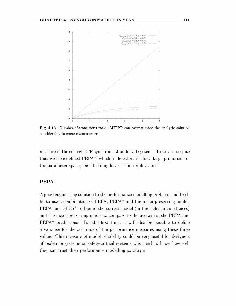
CHAPTER 4. SYNCHRONISATION IN SPAS 111
0
2
4
6
8
10
12
14
16
18
0 1 2 3 4 5
Fig. 4.13. Number-of-transitions ratio: MTIPP can overestimate the analytic solution
considerably in some circumstances.
measure of the correct LTF synchronisation for all systems. However, despite
this, we have de�ned PEPA*, which underestimates for a large proportion of
the parameter space, and this may have useful implications.
PEPA
A good engineering solution to the performance modelling problem could well
be to use a combination of PEPA, PEPA* and the mean-preserving model:
PEPA and PEPA* to bound the correct model (in the right circumstances)
and the mean-preserving model to compare to the average of the PEPA and
PEPA* predictions. For the �rst time, it will also be possible to de�ne
a variance for the accuracy of the performance measures using these three
values. This measure of model reliability could be very useful for designers
of real-time systems or safety-critical systems who need to know how well
they can trust their performance modelling paradigm.
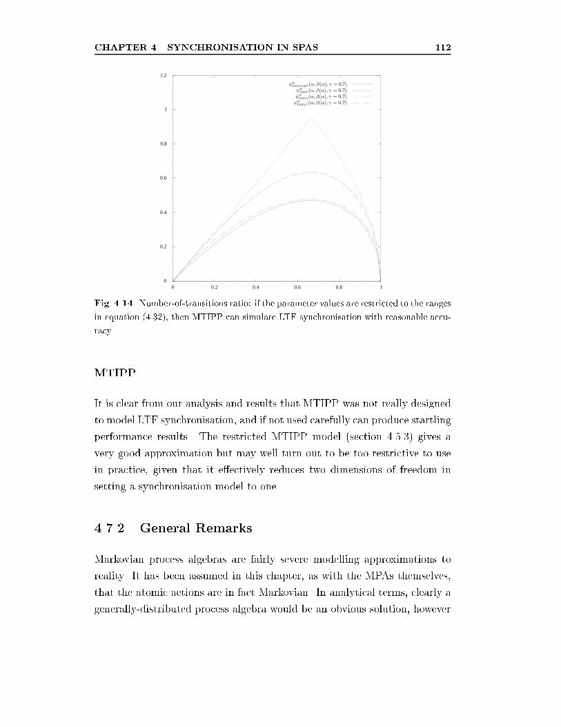
CHAPTER 4. SYNCHRONISATION IN SPAS 112
0
0.2
0.4
0.6
0.8
1
1.2
0 0.2 0.4 0.6 0.8 1
Fig. 4.14. Number-of-transitions ratio: if the parameter values are restricted to the ranges
in equation (4.32), then MTIPP can simulate LTF synchronisation with reasonable accu-
racy.
MTIPP
It is clear from our analysis and results that MTIPP was not really designed
to model LTF synchronisation, and if not used carefully can produce startling
performance results. The restricted MTIPP model (section 4.5.3) gives a
very good approximation but may well turn out to be too restrictive to use
in practice, given that it e�ectively reduces two dimensions of freedom in
setting a synchronisation model to one.
4.7.2 General Remarks
Markovian process algebras are fairly severe modelling approximations to
reality. It has been assumed in this chapter, as with the MPAs themselves,
that the atomic actions are in fact Markovian. In analytical terms, clearly a
generally-distributed process algebra would be an obvious solution, however

CHAPTER 4. SYNCHRONISATION IN SPAS 113
there is a paucity of techniques and tools for obtaining performance �gures for
large-scale systems. In the absence of such techniques and while Markovian
process algebra research into faster solution techniques continues to ourish,
an understanding of how to use MPAs in a reliable way can only be a good
thing.
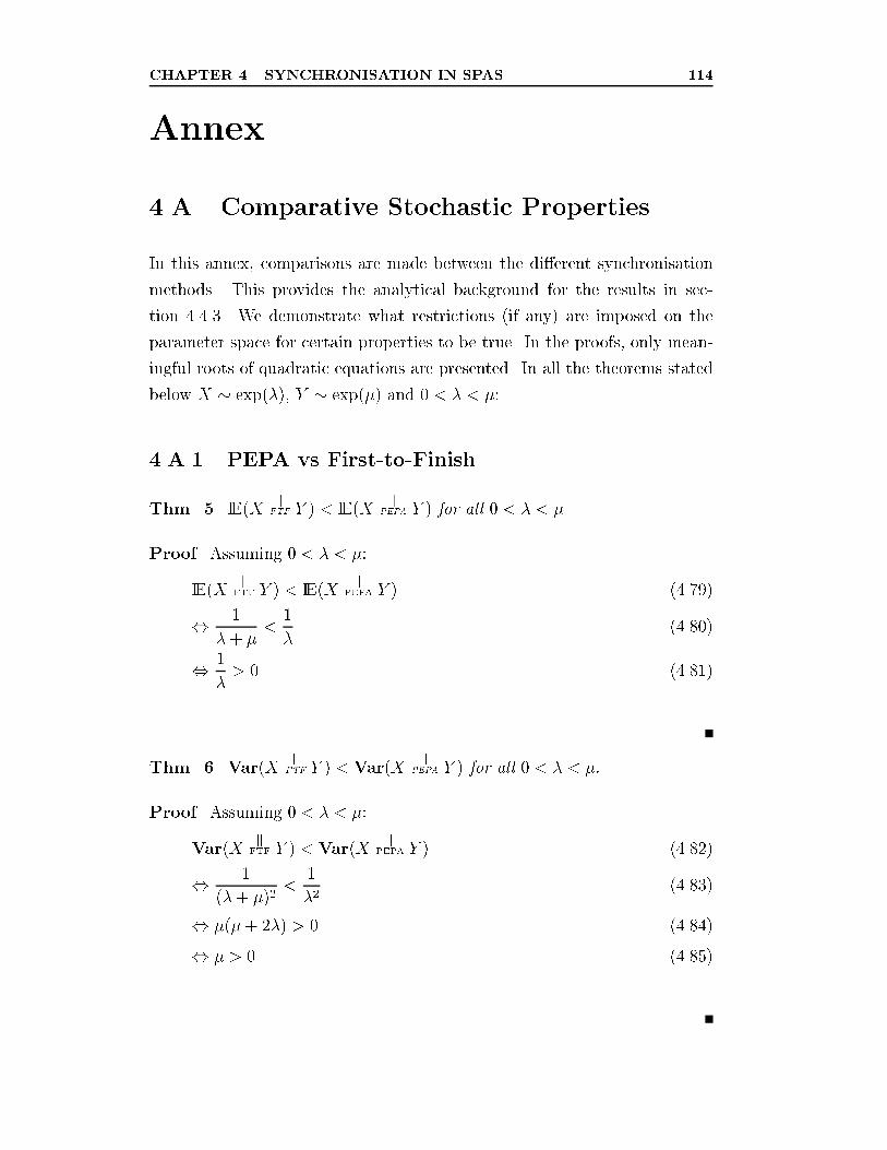
CHAPTER 4. SYNCHRONISATION IN SPAS 114
Annex
4.A Comparative Stochastic Properties
In this annex, comparisons are made between the di�erent synchronisation
methods. This provides the analytical background for the results in sec-
tion 4.4.3. We demonstrate what restrictions (if any) are imposed on the
parameter space for certain properties to be true. In the proofs, only mean-
ingful roots of quadratic equations are presented. In all the theorems stated
below X � exp(�), Y � exp(�) and 0 < � < �:
4.A.1 PEPA vs First-to-Finish
Thm. 5. IE(Xk
FTF Y ) < IE(Xk
PEPA Y ) for all 0 < � < �.
Proof. Assuming 0 < � < �:
IE(Xk
FTF Y ) < IE(Xk
PEPA Y ) (4.79)
, 1
�+ �<
1
�(4.80)
, 1
�> 0 (4.81)
Thm. 6. Var(Xk
FTF Y ) < Var(Xk
PEPA Y ) for all 0 < � < �:
Proof. Assuming 0 < � < �:
Var(Xk
FTF Y ) < Var(Xk
PEPA Y ) (4.82)
, 1
(�+ �)2<
1
�2(4.83)
, �(�+ 2�) > 0 (4.84)
, � > 0 (4.85)
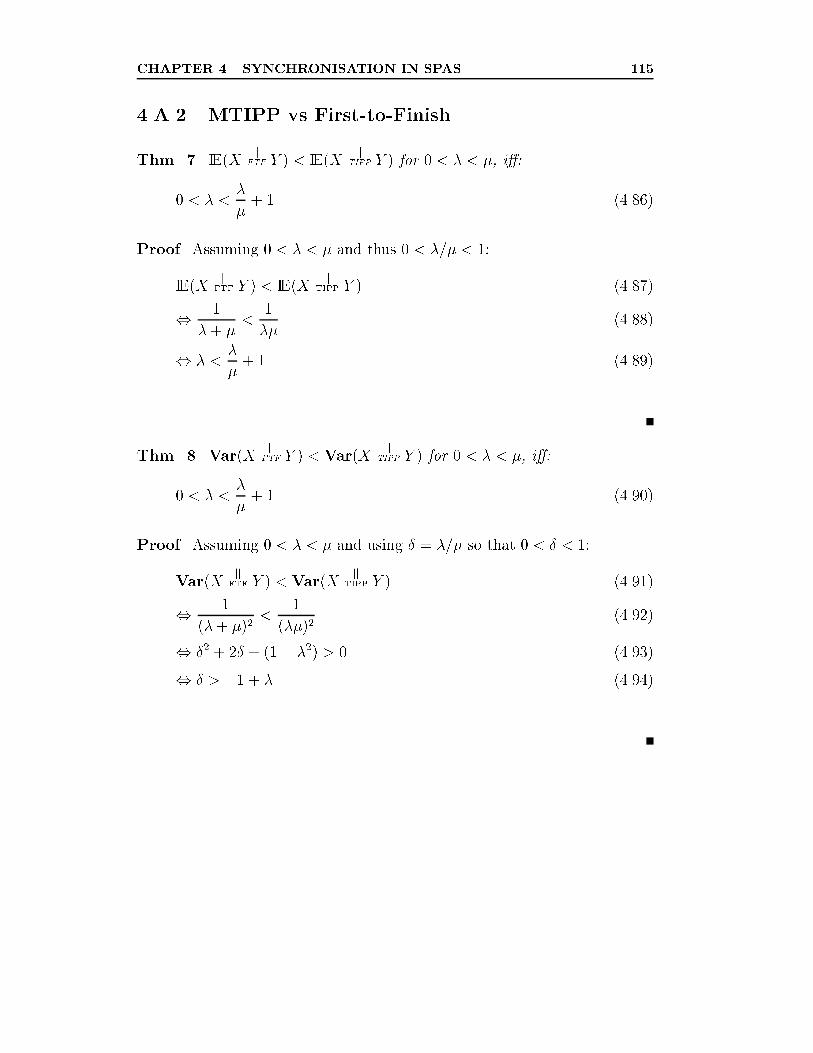
CHAPTER 4. SYNCHRONISATION IN SPAS 115
4.A.2 MTIPP vs First-to-Finish
Thm. 7. IE(Xk
FTF Y ) < IE(Xk
TIPP Y ) for 0 < � < �, i�:
0 < � <�
�+ 1 (4.86)
Proof. Assuming 0 < � < � and thus 0 < �=� < 1:
IE(Xk
FTF Y ) < IE(Xk
TIPP Y ) (4.87)
, 1
�+ �<
1
��(4.88)
, � <�
�+ 1 (4.89)
Thm. 8. Var(Xk
FTF Y ) < Var(Xk
TIPP Y ) for 0 < � < �, i�:
0 < � <�
�+ 1 (4.90)
Proof. Assuming 0 < � < � and using � = �=� so that 0 < � < 1:
Var(Xk
FTF Y ) < Var(Xk
TIPP Y ) (4.91)
, 1
(�+ �)2<
1
(��)2(4.92)
, �2 + 2� + (1� �2) > 0 (4.93)
, � > �1 + � (4.94)
CHAPTER 4. SYNCHRONISATION IN SPAS 116
4.A.3 PEPA vs Last-to-Finish
Thm. 9. IE(Xk
PEPA Y ) < IE(Xk
LTF Y ) for all 0 < � < �.
Proof. Assuming 0 < � < �:
IE(Xk
PEPA Y ) < IE(Xk
LTF Y ) (4.95)
, 1
�+
1
�� 1
�+ �>
1
�(4.96)
, � > 0 (4.97)
Thm. 10. Var(Xk
LTF Y ) < Var(Xk
PEPA Y ) for 0 < � < �, i�:
0 <�
�<p3� 1 (4.98)
Proof. Assuming 0 < � < � and � = �=� so that 0 < � < 1:
Var(Xk
LTF Y ) < Var(Xk
PEPA Y ) (4.99)
, 1
�2+
1
�2� 3
(�+ �)2<
1
�2(4.100)
, (�+ �)2 � 3�2 < 0 (4.101)
, 0 < � <p3� 1 (4.102)
4.A.4 MTIPP vs Last-to-Finish
Thm. 11. IE(Xk
LTF Y ) < IE(Xk
TIPP Y ) for 0 < � < �, i� both:
0 < � <2
3and
1
2
"�1 +
r1 + 3�
1� �
#<�
�< 1 (4.103)
CHAPTER 4. SYNCHRONISATION IN SPAS 117
Proof. Assuming 0 < � < � and using � = �=� so that 0 < � < 1:
IE(Xk
LTF Y ) < IE(Xk
TIPP Y ) (4.104)
, 1
�+
1
�� 1
�+ �<
1
��(4.105)
, (�� 1)�2 + (�� 1)� + � < 0 (4.106)
, � >1
2
"�1 +
r1 + 3�
1� �
#(4.107)
However, this root of � is only meaningful for � < 1, so combining the two
inequalities gives the additional condition, 0 < � < 2=3.
Thm. 12. Var(Xk
LTF Y ) < Var(Xk
TIPP Y ) for 0 < � < �, i� both:
0 < �� <4
5and 4 < <
(2� + 1) +p16�2 + 4� + 1
2�(4.108)
where = (�+ �)2=�, � = ��.
Proof. Using � = �=�, � = (� + �)2, � = ��, = �=� = � + 2 + ��1 and
assuming 0 < � < � and thus 0 < � < 1 and > 4:
Var(Xk
LTF Y ) < Var(Xk
TIPP Y ) (4.109)
, 1
�2+
1
�2� 3
(�+ �)2<
1
(��)2(4.110)
, �2 � 2�� � 3�2 � � < 0 (4.111)
, 2 � 2� + 1
� � 3 < 0 (4.112)
, <(2� + 1) +
p16�2 + 4� + 1
2�(4.113)
However, this root of is only meaningful for > 4, so combining the two
inequalities gives the additional condition, 0 < � < 4=5.
CHAPTER 4. SYNCHRONISATION IN SPAS 118
4.A.5 MTIPP vs PEPA
Thm. 13. IE(Xk
TIPP Y ) < IE(Xk
PEPA Y ) for 0 < � < �, i� � > 1.
Proof. Assuming 0 < � < �:
IE(Xk
TIPP Y < IE(Xk
PEPA Y ) (4.114)
, 1
��<
1
�(4.115)
, � > 1 (4.116)
Thm. 14. Var(Xk
TIPP Y ) < Var(Xk
PEPA Y ) for 0 < � < �, i� � > 1.
Proof. Assuming 0 < � < �:
Var(Xk
TIPP Y ) < Var(Xk
PEPA Y ) (4.117)
, 1
(��)2<
1
�2(4.118)
, � > 1 (4.119)

Chapter 5
Reliability of Models in SPAs
5.1 Introduction
Reliability is often seen as a cut-and-dried property. A computer model is
proposed, a reliability criterion is de�ned and the model is analysed against
that criterion to see whether it is or is not reliable. By de�ning a system with
a stochastic process algebra we have the opportunity to model the uncertainty
that, in reality, pervades today's communication networks and distributed
systems.
In this chapter, we concentrate on reliable models rather than the paradigm
itself. What seriously hinders stochastic modelling and simulation today
is the explosion in variance that can easily overtake a model and make it
analytically useless. If a system has large variations in temporal behaviour,
these will impinge on other systems with which it communicates, causing
them in turn to be unpredictable (if they are not speci�cally designed to
expect high variance communication). The whole system will take longer to
converge to any sort of equilibrium behaviour, if it ever converges at all. This
119
CHAPTER 5. RELIABILITY OF MODELS IN SPAS 120
has a direct corollary: it will be longer before any steady-state analysis has
any bearing on physical reality.
Systems which have small variation are therefore much easier to use from a
safety-critical point of view|their behaviour is nicely bounded and will not
cause other components to behave erratically.
Our brief in this chapter, then, is to investigate variance-management tech-
niques1 at the design stage of a system from a stochastic process algebra
perspective. We construct a simple stochastic process algebra which embod-
ies the properties that we have identi�ed as being important to modelling
expressively and reliably (using multiple synchronisation types and modelling
with general distributions). We develop a simple framework for interpreting
SPAs in terms of reliable behaviour and variance. We go on to demonstrate
how this property changes under combination of the SPA operators.
By targeting variance reduction in a modelling environment such as stochas-
tic process algebras, we aim to give the modeller a set of tools by which they
can know how to reduce variance and increase global system predictability.
We go some way towards that goal in this chapter, but also demonstrate
some of the issues that make it di�cult to achieve in general.
We �nish by analysing two examples in terms of reliability: a searching prob-
lem (section 5.5.1 and originally presented in [13]) and a model of a telephone
communication system (section 5.5.2). Finally, we explore what can currently
be achieved with reliable modelling techniques and SPAs, informed by the
results of this chapter.
5.2 De�nitions of Reliability
As we have seen in chapter 2, from an SPA point-of-view reliability is a
slightly alien concept. It is generally considered a hard enough problem to
1This typically, but not always, means reducing variance. In the event that variance
needs to be increased in a system, we will see that this can be achieved easily.
CHAPTER 5. RELIABILITY OF MODELS IN SPAS 121
obtain average behaviour for a stochastically de�ned system without having
to worry about obtaining other measures. As a result, it is di�cult to see
how reliability could be extracted from current solution techniques which are
centred around �nding steady-state probabilities.
In a performance context, knowing how much a system can vary from its
mean performance is an essential practical consideration. Or indeed, to put
it the other way round, if the variation of behaviour is very large then having
only the mean �gure for a sojourn is probably not much use for analysis.
So, how to de�ne reliability in the context of a stochastically de�ned system?
If we consider a �nite path in a stochastic transition system, we can aggregate
the random variables that make up the path and obtain a distribution for the
entire path [12]. This distribution will have a mean, a variance and all the
higher moments; as a starting point the variance will be a useful reliability
statistic to gather. A path with large variance will slow down a system's
convergence to stationary behaviour, whereas a path with small variance
will make the system more predictable (or deterministic).
However, if we are able to derive the distribution completely for such a path,
this represents a better measure of the path's reliability. If the distribution
were asymmetric, for instance, this would be evident from the distribution
but not re ected in the variance.
In the course of this chapter, we will look at both aggregate distributions and
variances. We will discover that general statements about reliability can be
made according to how systems are constructed. In particular, the type of
operator and modelling strategy used can dramatically a�ect the predicted
reliability of a system.
5.2.1 Real-Time Systems
For systems for which reliability is important, average long-term behaviour
is not the primary issue: hazards may occur or functionality may be at risk
if individual instances of operation fall outside certain bounds. We want to
CHAPTER 5. RELIABILITY OF MODELS IN SPAS 122
be able to reason about local or transient behaviour as well as operation in
the long term.
For instance, if we have a time-out race between an exponentially distributed
action, X � exp(10), and a deterministic cut-o�, Y � �(10), if the time-out,
Y , occurs �rst the system might well go into some kind of failure mode or
error handler or may just deadlock. We need to be able to ascertain the
probability of the system going into such a state every time it goes into this
time-out:
P (X > Y ) = P (X > 10) = FX(10) = e�100 (5.1)
Such vanishingly small probabilities might form the basis of a safety case or
an industrial standard for a component or hazard situation.
In MTL [72] (a real-time modelling algebra), typically, such local behaviour
is looked at by examining the interval between two events where each event in
the system is given a �xed duration. Similarly in TIS [90] (another real-time
modelling language), for example, speci�c amounts of time are allocated to
actions of a model. Veri�cation takes the form of asking whether intervals of
operation take less than or greater than a hard bound.
In a stochastic system we can use the notion of stochastic aggregation [12]
to produce a similar, but stochastically de�ned, result. Given a distribution
for a particular interval, how might reliability be de�ned on it? Various TIS
papers [90, 89, 100] have a categorisation of reliable probabilistic operation,
which can basically be summarised into two categories:
1. One-tailed test: P (X < a) = p or P (X > b) = q
2. Two-tailed test: P (a < X < b) = p
where a, b, p and q would be speci�ed for necessary reliable behaviour. These
are easily attainable from the cumulative distribution function of an aggre-
gate distribution. However, given that TIS itself speci�es exact durations,
it is not able to obtain these quantities on a given path|it has to settle for
obtaining deterministic or hard bounds on path execution.
CHAPTER 5. RELIABILITY OF MODELS IN SPAS 123
5.2.2 Variance in Stochastic Transition Systems
A second idea is to use the aggregation method again, but this time calculate
the variance and then, easily, the coe�cient of variation, CX :
CX =
pVar(X)
IE(X)(5.2)
This is particularly attractive since it not only gives an idea of how \con-
centrated" or \di�use" a distribution might be (which is a good measure of
determinism) but also allows us to aggregate in Laplace-space and generate
the moments from the Laplace transform of the aggregate distribution [97].
Thus an inversion of a Laplace transform and an integration to the cumula-
tive distribution function are avoided.
Let us consider the following stochastic transition system (similar to that
from chapter 3) where each transition has a random variable, X, attributed
to its execution:
P ::= 0 fXg:P [m]P � [1�m]P (5.3)
This represents a stochastic component where either transitions occur, taking
a random amount of time, or a probabilistic branch occurs with probability
m for one path and (1�m) for the other.
Just by considering the variance of certain stochastic paths, we can gain
some interesting insight. Take the following reliability function, V0, which
measures the variance of a terminating path, V0 : P �! IR:
V0(0) = 0 (5.4)
V0(fXg:P ) = Var(X) + V0(P ) (5.5)
V0([m]P � [1�m]Q) = mV0(P ) + (1�m)V0(Q)
+m(1�m)(E0(P )� E0(Q))2
(5.6)
CHAPTER 5. RELIABILITY OF MODELS IN SPAS 124
where E0 : P �! IR represents the mean time of path execution:
E0(0) = 0 (5.7)
E0(fXg:P ) = IE(X) + E0(P ) (5.8)
E0([m]P � [1�m]Q) = mE0(P ) + (1�m)E0(Q) (5.9)
where IE(X) is the mean, as before, and Var(X) is the variance of a random
variable X. Equation (5.5) is essentially a result of the convolution formula
and shows that a �nite system which is described by nothing but a sequence
of events will have a monotonically increasing variance. Equation (5.6) repre-
sents the formula for a probabilistic branch [97] and shows that this is where
variance reduction might be achieved within a stochastic system.
This is the premise of the chapter: many systems are largely sequential and
this leads to the variance explosion problem, when modelling or simulating
systems. The fact that probabilistic branching (and thus other constructs
like competitive choice and synchronisations, which, from chapter 3, we know
can be expressed in terms of probabilistic branching [16]) can reduce vari-
ance, means that there is a possibility of reducing this explosion. We will
demonstrate that this is so in the next section.
5.3 A General Stochastic Process Algebra
5.3.1 De�nition
If we are to take a process algebra perspective on reliability in models of
communicating systems, then we clearly need a process algebra to work on.
As we have seen from our discussion of chapter 3, traditional analysis of
generally distributed stochastic process algebras (obtaining stationary distri-
butions) can prove very di�cult. However, �nding stationary distributions
is of limited usefulness from a reliability modelling point of view.
This gives us an opportunity to de�ne other analysis techniques on a generally
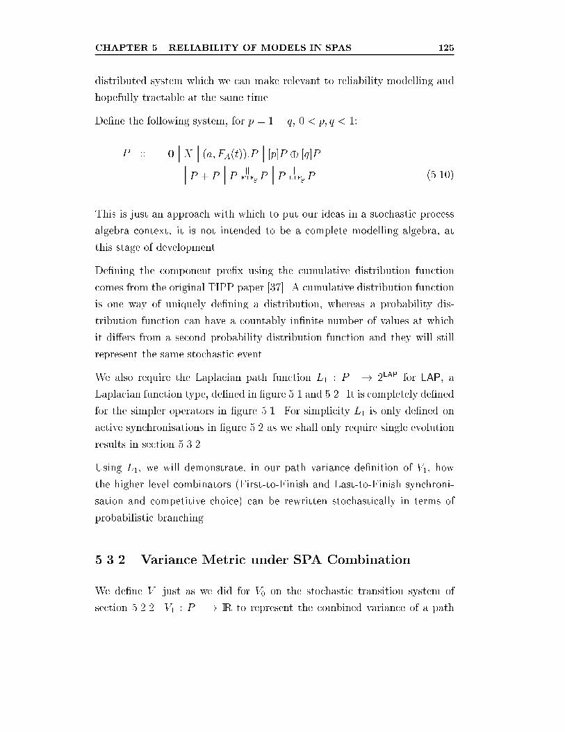
CHAPTER 5. RELIABILITY OF MODELS IN SPAS 125
distributed system which we can make relevant to reliability modelling and
hopefully tractable at the same time.
De�ne the following system, for p = 1� q, 0 < p; q < 1:
P ::= 0 X (a; FA(t)):P [p]P � [q]P
P + P Pk
FTFSP P
kLTF
SP (5.10)
This is just an approach with which to put our ideas in a stochastic process
algebra context, it is not intended to be a complete modelling algebra, at
this stage of development.
De�ning the component pre�x using the cumulative distribution function
comes from the original TIPP paper [37]. A cumulative distribution function
is one way of uniquely de�ning a distribution, whereas a probability dis-
tribution function can have a countably in�nite number of values at which
it di�ers from a second probability distribution function and they will still
represent the same stochastic event.
We also require the Laplacian path function L1 : P �! 2LAP for LAP, a
Laplacian function type, de�ned in �gure 5.1 and 5.2. It is completely de�ned
for the simpler operators in �gure 5.1. For simplicity L1 is only de�ned on
active synchronisations in �gure 5.2 as we shall only require single evolution
results in section 5.3.2.
Using L1, we will demonstrate, in our path variance de�nition of V1, how
the higher level combinators (First-to-Finish and Last-to-Finish synchroni-
sation and competitive choice) can be rewritten stochastically in terms of
probabilistic branching.
5.3.2 Variance Metric under SPA Combination
We de�ne V1 just as we did for V0 on the stochastic transition system of
section 5.2.2. V1 : P �! IR to represent the combined variance of a path
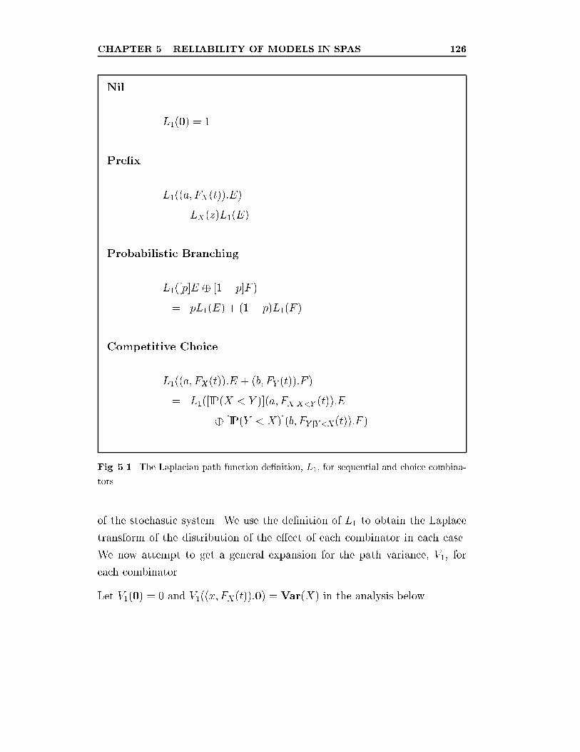
CHAPTER 5. RELIABILITY OF MODELS IN SPAS 126
Nil
L1(0) = 1
Pre�x
L1((a; FX(t)):E)
= LX(z)L1(E)
Probabilistic Branching
L1([p]E � [1� p]F )= pL1(E) + (1� p)L1(F )
Competitive Choice
L1((a; FX(t)):E + (b; FY (t)):F )
= L1([IP(X < Y )](a; FXjX<Y (t)):E
� [IP(Y < X)](b; FY jY <X(t)):F )
Fig. 5.1. The Laplacian path function de�nition, L1, for sequential and choice combina-
tors.
of the stochastic system. We use the de�nition of L1 to obtain the Laplace
transform of the distribution of the e�ect of each combinator in each case.
We now attempt to get a general expansion for the path variance, V1, for
each combinator.
Let V1(0) = 0 and V1((x; FX(t)):0) = Var(X) in the analysis below.
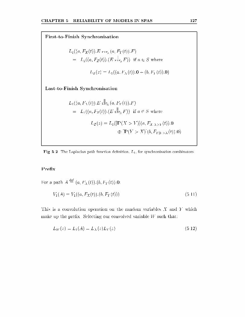
CHAPTER 5. RELIABILITY OF MODELS IN SPAS 127
First-to-Finish Synchronisation
L1((a; FX(t)):Ek
FTFS(a; FY (t)):F )
= L1((a; FZ(t)):(Ek
FTFSF )) if a 2 S where
LZ(z) = L1((a; FX(t)):0+ (b; FY (t)):0)
Last-to-Finish Synchronisation
L1((a; FX(t)):Ek
LTFS(a; FY (t)):F )
= L1((a; FZ(t)):(Ek
LTFSF )) if a 2 S where
LZ(z) = L1([IP(X > Y )](a; FXjX>Y (t)):0
� [IP(Y > X)](b; FY jY >X(t)):0)
Fig. 5.2. The Laplacian path function de�nition, L1, for synchronisation combinators.
Pre�x
For a path Adef= (a; FX(t)):(b; FY (t)):0:
V1(A) = V1((a; FX(t)):(b; FY (t))) (5.11)
This is a convolution operation on the random variables X and Y which
make up the pre�x. Selecting our convolved variable W such that:
LW (z) = L1(A) = LX(z)LY (z) (5.12)
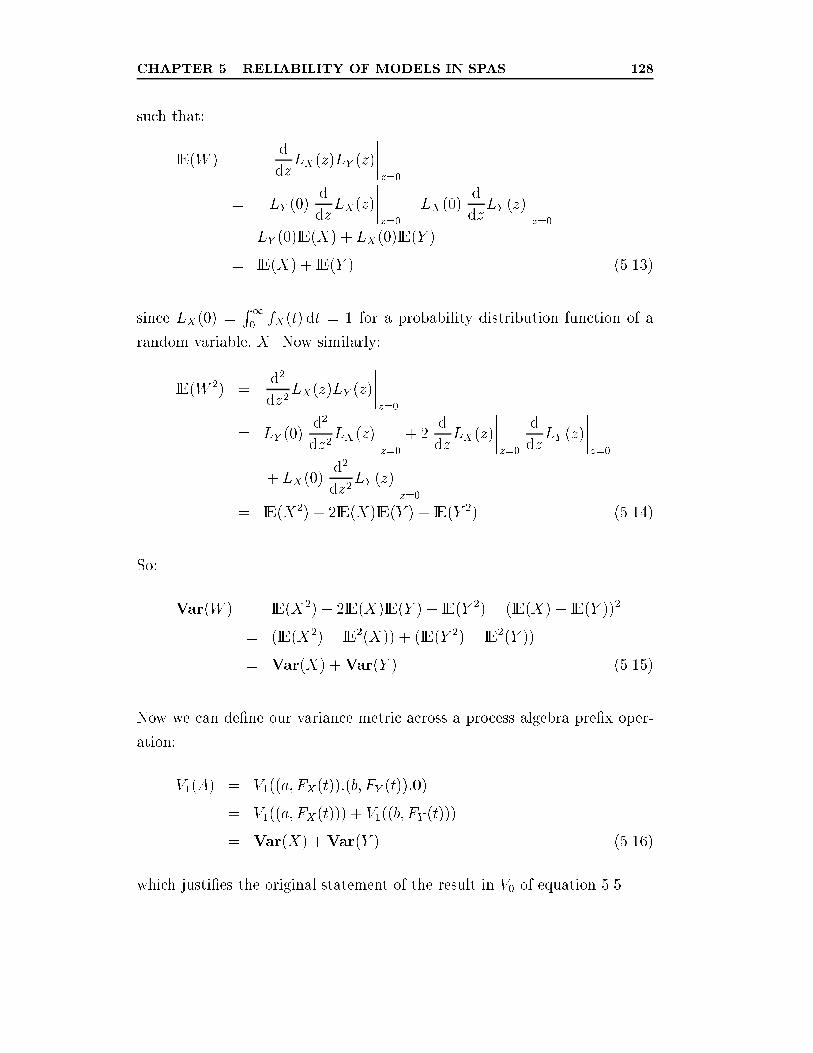
CHAPTER 5. RELIABILITY OF MODELS IN SPAS 128
such that:
IE(W ) = � d
dzLX(z)LY (z)
����z=0
= �LY (0) d
dzLX(z)
����z=0
� LX(0) d
dzLY (z)
����z=0
= LY (0)IE(X) + LX(0)IE(Y )
= IE(X) + IE(Y ) (5.13)
since LX(0) =R10fX(t) dt = 1 for a probability distribution function of a
random variable, X. Now similarly:
IE(W 2) =d2
dz 2LX(z)LY (z)
����z=0
= LY (0)d2
dz 2LX(z)
����z=0
+ 2d
dzLX(z)
����z=0
d
dzLY (z)
����z=0
+ LX(0)d2
dz 2LY (z)
����z=0
= IE(X2) + 2IE(X)IE(Y ) + IE(Y 2) (5.14)
So:
Var(W ) = IE(X2) + 2IE(X)IE(Y ) + IE(Y 2)� (IE(X) + IE(Y ))2
= (IE(X2)� IE2(X)) + (IE(Y 2)� IE2(Y ))
= Var(X) +Var(Y ) (5.15)
Now we can de�ne our variance metric across a process algebra pre�x oper-
ation:
V1(A) = V1((a; FX(t)):(b; FY (t)):0)
= V1((a; FX(t))) + V1((b; FY (t)))
= Var(X) +Var(Y ) (5.16)
which justi�es the original statement of the result in V0 of equation 5.5.
CHAPTER 5. RELIABILITY OF MODELS IN SPAS 129
Probabilistic Branching
For a path Adef= [p](a; FX(t)):0 � [q](b; FY (t)):0, where W represents the
stochastic aggregation of the system A:
LW (z) = L1(A) = pLX(t) + qLY (t) (5.17)
IE(W ) = pIE(X) + qIE(Y ) (5.18)
IE(W 2) = pIE(X2) + qIE(Y 2) (5.19)
Var(W ) = pIE(X2) + qIE(Y 2)� p2IE2(X)� q2IE(Y )� 2pqIE(X)IE(Y )
= pVar(X) + pqIE2(X) + qVar(Y ) + pqIE2(Y )
� 2pqIE(X)IE(Y )
= pVar(X) + qVar(Y ) + pq(IE(X)� IE(Y ))2 (5.20)
So we de�ne V1 over probabilistic branching as follows:
V1(A) = V1([p](a; FX(t)):0� [q](b; FY (t)):0)
= pVar(X) + qVar(Y ) + pq(IE(X)� IE(Y ))2 (5.21)
which again justi�es V0, equation (5.6).
Competitive Choice and First-to-Finish Synchronisation
From the de�nition of L1, we know that, stochastically speaking, competitive
choice and First-to-Finish synchronisation are the same. They, of course, dif-
fer in operational terms since, as the �rst process terminates, the competitive
choice operator terminates the slower process whereas the synchronisation
operator pre-empts the other process but thereafter allows it to continue. In
both cases, though, the time taken is equal to that of the faster process.
CHAPTER 5. RELIABILITY OF MODELS IN SPAS 130
Thus for:
Adef= (a; FX(t)):0 + (b; FY (t)):0 (5.22)
Bdef= (a; FX(t)):0
kFTFfag (a; FY (t)):0 (5.23)
V1(A) = V1(B) since L1(A) = L1(B). Now, directly from the de�nition of
L1, we can say:
V1(A) = IP(X < Y )Var(XjX < Y ) + IP(Y < X)Var(Y jY < X)
+ IP(X < Y )IP(Y < X)(IE(XjX < Y )� IE(Y jY < X))2
(5.24)
This does not seem to be reducible to an expression involving just terms
Var(X), Var(Y ) and IE(X), IE(Y ) in general. Thus in the next section we
investigate synchronisations with speci�c common modelling distributions.
Last-to-Finish Synchronisation
From our stochastic de�nition of LTF synchronisation, L1, we can use the
probabilistic branch result to give us a general formula for a Last-to-Finish
synchronisation, Adef= (a; FX(t)):0
kLTFfag (a; FY (t)):0 and so:
V1(A) = IP(X > Y )Var(XjX > Y ) + IP(Y > X)Var(Y jY > X)
+ IP(X > Y )IP(Y > X)(IE(XjX > Y )� IE(Y jY > X))2
(5.25)
Similarly, this does not appear to be reducible to an expression involving just
terms Var(X), Var(Y ) and IE(X), IE(Y ) in general, and so we are forced to
derive conclusions from speci�c distribution examples in section 5.4.
CHAPTER 5. RELIABILITY OF MODELS IN SPAS 131
5.4 Speci�c Distributions under SPA
Combination
In the following section we look at how speci�c distributions are a�ected by
stochastic process algebra combinators, like competitive choice and Last-to-
Finish synchronisation. We will examine variance properties of some of the
simpler distributions in combinations:
Dirac delta function which represents deterministic behaviour in a stoch-
astic environment. It is used in models of the ATM protocol to repre-
sent a deterministic service process in a switch. Also, more generally,
it can represent a deterministic time-out of a late process.
Exponential distribution which, although arguably overused in stochas-
tic modelling, does have real-world applicability. As we will see a
na��vely implemented algorithm can easily have an exponentially dis-
tributed time-to-�nish. Also, as we are not necessarily interested solely
in computer systems, but in process modelling in general, many natu-
rally occurring phenomena can occur with an exponential distribution.
Uniform distribution represents bounded random events. It is an easy
way of expressing an approximation to an event which, it is known,
must occur between two time values.
The study of these distributions is motivated by their practical application,
discussed above, and, practically speaking, because they are easier to analyse
than some of the more complex multi-parameter distributions.
We cannot claim any kind of complete taxonomy with the analysis in the
sections to come. However, we hope to motivate discussion of speci�c distri-
butions or sets of distributions which will be of real modelling value if some
closed-form solution could be obtained. Ultimately this is probably one of
the main goals of reliability analysis using stochastic processes and stochastic
CHAPTER 5. RELIABILITY OF MODELS IN SPAS 132
process algebras|the ability to be able to say that using a speci�c distri-
bution set under a speci�c combinator, the reliability and predictability of
an overall system will be improved. Obviously from a modelling perspective
the broader that set of distributions, the more descriptive the paradigm and
the more useful it can be. Ideally, if general reliability statements could be
made about, say, a combination of Coxian stage-type distributions, then that
would give us a great deal of descriptive power, but as we will see, even for
something as simple as relative variance, making general statements about
even simple distributions is quite di�cult.
The analysis below considers the e�ect on path variance of speci�c com-
binations of commonly occurring distributions. Speci�cally, we consider a
primary distribution which is then combined with a second distribution un-
der a particular discipline; we then compare the overall variance of the event
with that of the primary distribution.
The di�culty of obtaining general variance results for these more complex
combinators and indeed for any more complex distribution types is very
much a limiting factor of this analysis. However, we feel that, given the
physical importance of the distributions under consideration and the obvious
usefulness of the combinators, including these more specialised results is still
of use to the modeller and does add to the understanding of the subject.
The analysis for each pair of distributions takes three parts: the �rst ex-
tracts the variance of the combined distribution; the second, where possible,
extracts any general analytic conclusions that can be drawn from comparing
the overall path variance with that of the primary distribution; and �nally,
the third includes a plot of di�erential variance ranging over a key parameter.
For the higher level combinators below, we use the stochastic results for
min(X; Y ) and max(X; Y ) in terms of cumulative density functions, from
chapter 4. They are identical to the expressions we used in L1 to obtain
a general case (as proved in annex 5.B), but were easier to obtain speci�c
distribution results from. We also refer forward to the annex 5.A, in order
to use the single-distribution-speci�c results.
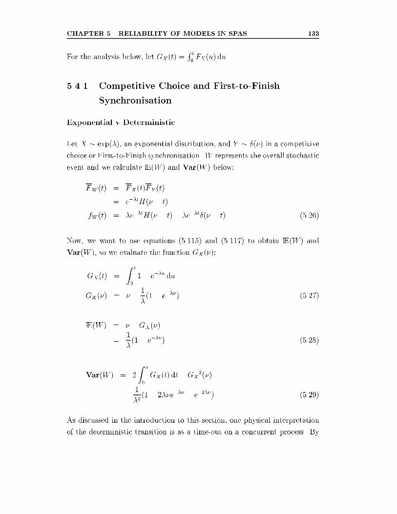
CHAPTER 5. RELIABILITY OF MODELS IN SPAS 133
For the analysis below, let GX(t) =R t0FX(u) du.
5.4.1 Competitive Choice and First-to-Finish
Synchronisation
Exponential v Deterministic
Let X � exp(�), an exponential distribution, and Y � �(�) in a competitive
choice or First-to-Finish synchronisation. W represents the overall stochastic
event and we calculate IE(W ) and Var(W ) below:
FW (t) = FX(t)F Y (t)
= e��tH(� � t)fW (t) = �e��tH(� � t) + �e��t�(� � t) (5.26)
Now, we want to use equations (5.115) and (5.117) to obtain IE(W ) and
Var(W ), so we evaluate the function GX(�):
GX(t) =
Z t
0
1� e��u du
GX(�) = � � 1
�(1� e���) (5.27)
IE(W ) = � �GX(�)
=1
�(1� e���) (5.28)
Var(W ) = 2
Z �
0
GX(t) dt�GX2(�)
=1
�2(1� 2��e��� � e�2��) (5.29)
As discussed in the introduction to this section, one physical interpretation
of the deterministic transition is as a time-out on a concurrent process. By
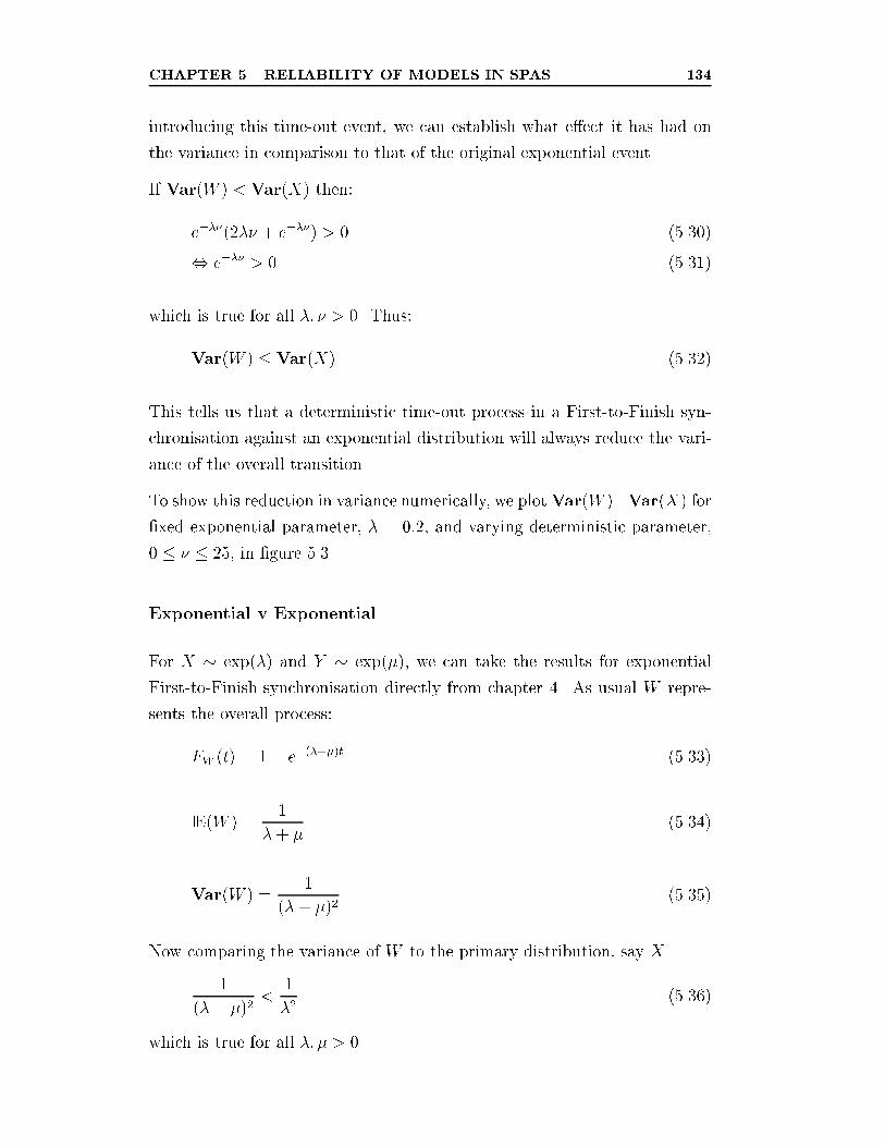
CHAPTER 5. RELIABILITY OF MODELS IN SPAS 134
introducing this time-out event, we can establish what e�ect it has had on
the variance in comparison to that of the original exponential event.
If Var(W ) < Var(X) then:
e���(2�� + e���) > 0 (5.30)
, e��� > 0 (5.31)
which is true for all �; � > 0. Thus:
Var(W ) � Var(X) (5.32)
This tells us that a deterministic time-out process in a First-to-Finish syn-
chronisation against an exponential distribution will always reduce the vari-
ance of the overall transition.
To show this reduction in variance numerically, we plotVar(W )�Var(X) for
�xed exponential parameter, � = 0:2, and varying deterministic parameter,
0 � � � 25, in �gure 5.3.
Exponential v Exponential
For X � exp(�) and Y � exp(�), we can take the results for exponential
First-to-Finish synchronisation directly from chapter 4. As usual W repre-
sents the overall process:
FW (t) = 1� e�(�+�)t (5.33)
IE(W ) =1
�+ �(5.34)
Var(W ) =1
(�+ �)2(5.35)
Now comparing the variance of W to the primary distribution, say X.
1
(�+ �)2<
1
�2(5.36)
which is true for all �; � > 0.
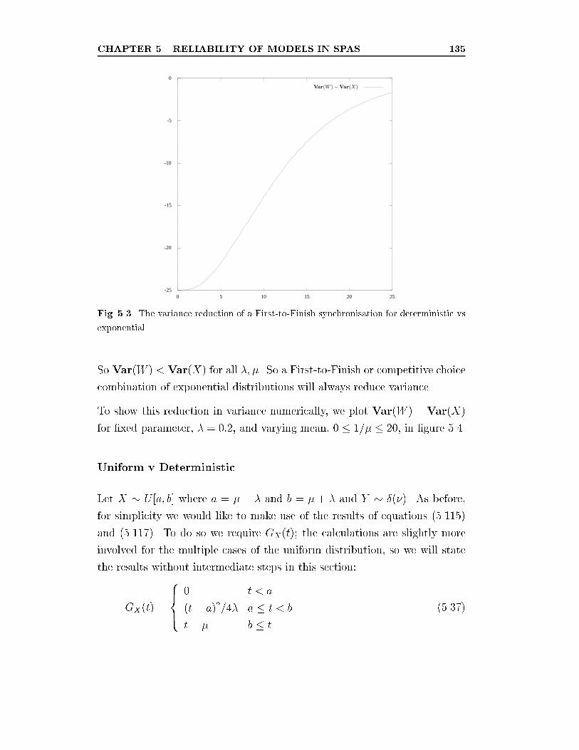
CHAPTER 5. RELIABILITY OF MODELS IN SPAS 135
-25
-20
-15
-10
-5
0
0 5 10 15 20 25
Fig. 5.3. The variance reduction of a First-to-Finish synchronisation for deterministic vs
exponential.
So Var(W ) < Var(X) for all �; �. So a First-to-Finish or competitive choice
combination of exponential distributions will always reduce variance.
To show this reduction in variance numerically, we plot Var(W )�Var(X)
for �xed parameter, � = 0:2, and varying mean, 0 � 1=� � 20, in �gure 5.4.
Uniform v Deterministic
Let X � U [a; b] where a = � � � and b = � + � and Y � �(�). As before,
for simplicity we would like to make use of the results of equations (5.115)
and (5.117). To do so we require GX(t); the calculations are slightly more
involved for the multiple cases of the uniform distribution, so we will state
the results without intermediate steps in this section:
GX(t) =
8><>:
0 t < a
(t� a)2=4� a � t < b
t� � b � t
(5.37)
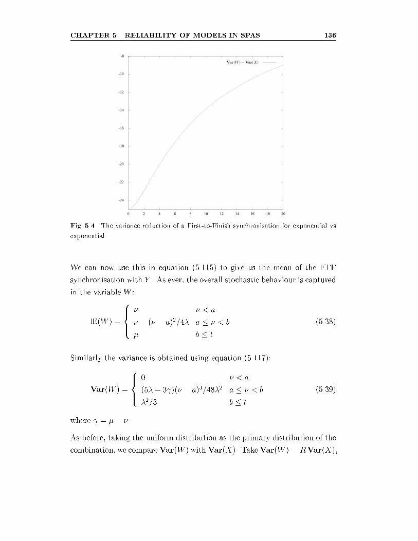
CHAPTER 5. RELIABILITY OF MODELS IN SPAS 136
-24
-22
-20
-18
-16
-14
-12
-10
-8
0 2 4 6 8 10 12 14 16 18 20
Fig. 5.4. The variance reduction of a First-to-Finish synchronisation for exponential vs
exponential.
We can now use this in equation (5.115) to give us the mean of the FTF
synchronisation with Y . As ever, the overall stochastic behaviour is captured
in the variable W :
IE(W ) =
8><>:
� � < a
� � (� � a)2=4� a � � < b
� b � t
(5.38)
Similarly the variance is obtained using equation (5.117):
Var(W ) =
8><>:
0 � < a
(5�+ 3 )(� � a)3=48�2 a � � < b
�2=3 b � t
(5.39)
where = �� �.As before, taking the uniform distribution as the primary distribution of the
combination, we compareVar(W ) withVar(X). TakeVar(W ) = RVar(X),
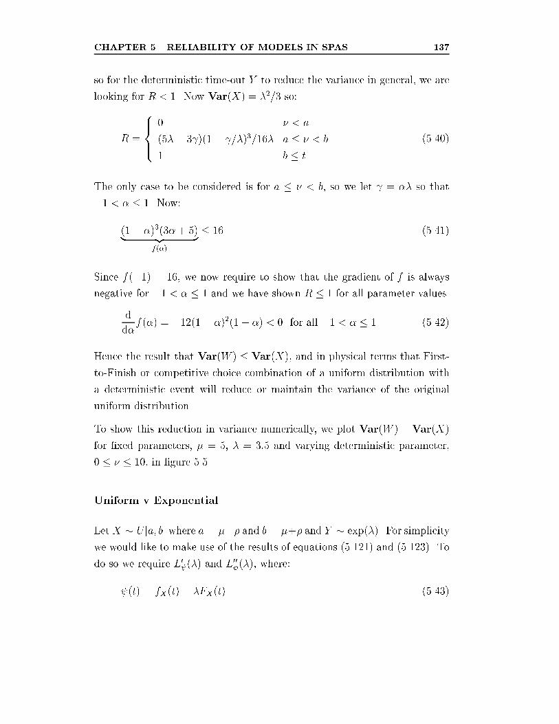
CHAPTER 5. RELIABILITY OF MODELS IN SPAS 137
so for the deterministic time-out Y to reduce the variance in general, we are
looking for R < 1. Now Var(X) = �2=3 so:
R =
8><>:
0 � < a
(5�+ 3 )(1� =�)3=16� a � � < b
1 b � t
(5.40)
The only case to be considered is for a � � < b, so we let = �� so that
�1 < � � 1. Now:
(1� �)3(3�+ 5)| {z }f(�)
� 16 (5.41)
Since f(�1) = 16, we now require to show that the gradient of f is always
negative for �1 < � � 1 and we have shown R � 1 for all parameter values.
d
d�f(�) = �12(1� �)2(1 + �) < 0 for all �1 < � � 1 (5.42)
Hence the result that Var(W ) � Var(X), and in physical terms that First-
to-Finish or competitive choice combination of a uniform distribution with
a deterministic event will reduce or maintain the variance of the original
uniform distribution.
To show this reduction in variance numerically, we plot Var(W )�Var(X)
for �xed parameters, � = 5, � = 3:5 and varying deterministic parameter,
0 � � � 10, in �gure 5.5.
Uniform v Exponential
LetX � U [a; b] where a = ��� and b = �+� and Y � exp(�). For simplicity
we would like to make use of the results of equations (5.121) and (5.123). To
do so we require L0 (�) and L00 (�), where:
(t) = fX(t)� �FX(t) (5.43)
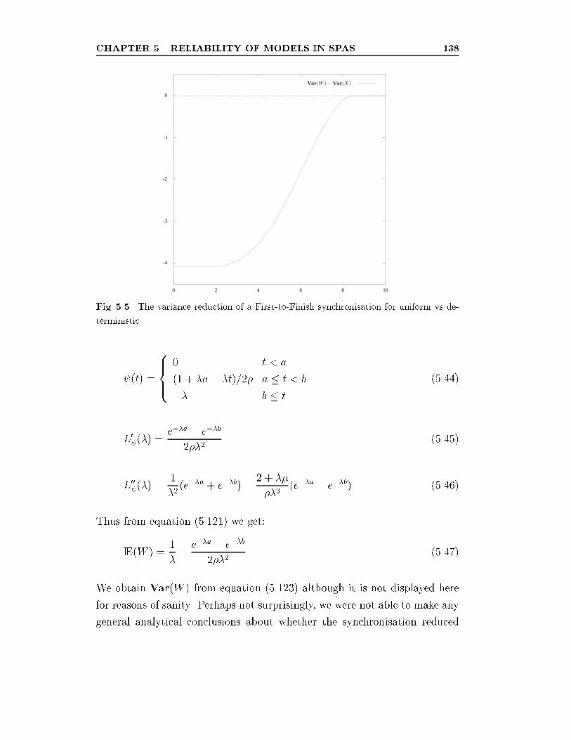
CHAPTER 5. RELIABILITY OF MODELS IN SPAS 138
-4
-3
-2
-1
0
0 2 4 6 8 10
Fig. 5.5. The variance reduction of a First-to-Finish synchronisation for uniform vs de-
terministic.
(t) =
8><>:
0 t < a
(1 + �a� �t)=2� a � t < b
�� b � t
(5.44)
L0 (�) =e��a � e��b
2��2(5.45)
L00 (�) =1
�2(e��a + e��b)� 2 + ��
��3(e��a � e��b) (5.46)
Thus from equation (5.121) we get:
IE(W ) =1
�� e��a � e��b
2��2(5.47)
We obtain Var(W ) from equation (5.123) although it is not displayed here
for reasons of sanity. Perhaps not surprisingly, we were not able to make any
general analytical conclusions about whether the synchronisation reduced
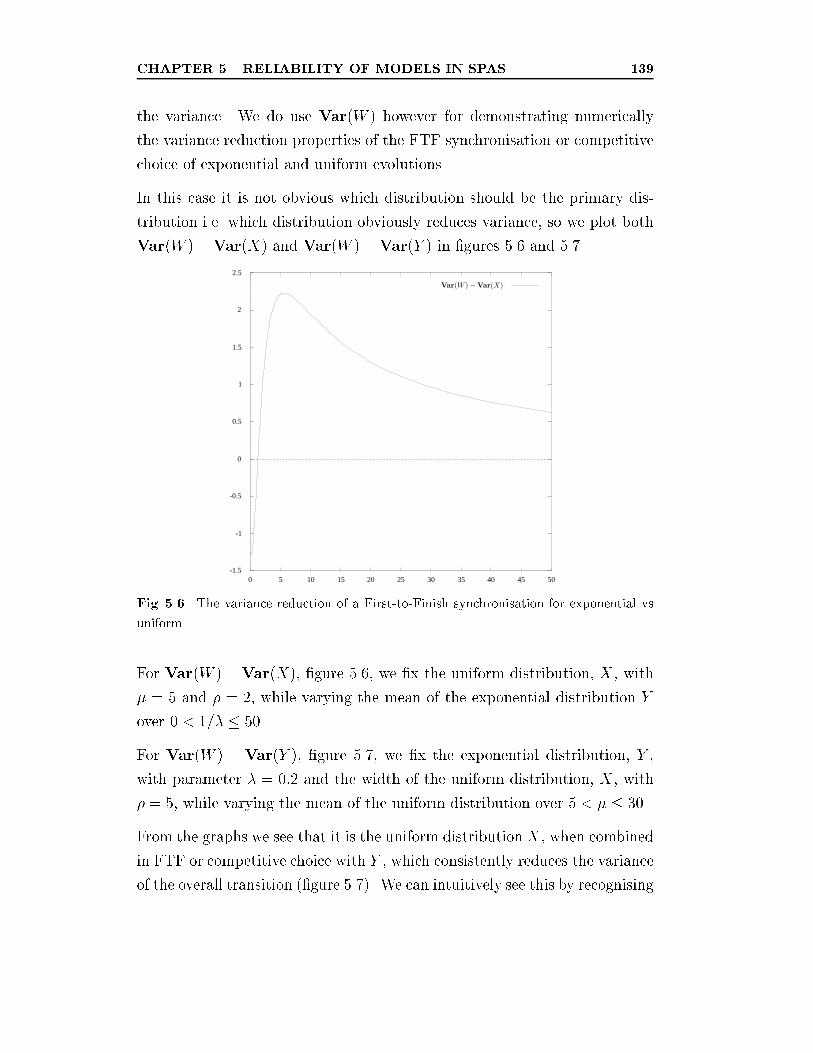
CHAPTER 5. RELIABILITY OF MODELS IN SPAS 139
the variance. We do use Var(W ) however for demonstrating numerically
the variance reduction properties of the FTF synchronisation or competitive
choice of exponential and uniform evolutions.
In this case it is not obvious which distribution should be the primary dis-
tribution i.e. which distribution obviously reduces variance, so we plot both
Var(W )�Var(X) and Var(W )�Var(Y ) in �gures 5.6 and 5.7.
-1.5
-1
-0.5
0
0.5
1
1.5
2
2.5
0 5 10 15 20 25 30 35 40 45 50
Fig. 5.6. The variance reduction of a First-to-Finish synchronisation for exponential vs
uniform.
For Var(W )�Var(X), �gure 5.6, we �x the uniform distribution, X, with
� = 5 and � = 2, while varying the mean of the exponential distribution Y
over 0 < 1=� � 50.
For Var(W ) � Var(Y ), �gure 5.7, we �x the exponential distribution, Y ,
with parameter � = 0:2 and the width of the uniform distribution, X, with
� = 5, while varying the mean of the uniform distribution over 5 < � � 30.
From the graphs we see that it is the uniform distributionX, when combined
in FTF or competitive choice with Y , which consistently reduces the variance
of the overall transition (�gure 5.7). We can intuitively see this by recognising
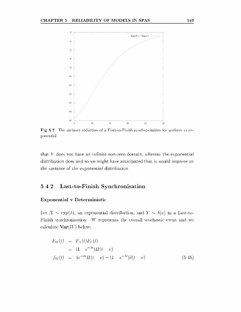
CHAPTER 5. RELIABILITY OF MODELS IN SPAS 140
-20
-18
-16
-14
-12
-10
-8
-6
-4
-2
0
5 10 15 20 25 30
Fig. 5.7. The variance reduction of a First-to-Finish synchronisation for uniform vs ex-
ponential.
that Y does not have an in�nite non-zero domain, whereas the exponential
distribution does and so we might have anticipated that it would improve on
the variance of the exponential distribution.
5.4.2 Last-to-Finish Synchronisation
Exponential v Deterministic
Let X � exp(�), an exponential distribution, and Y � �(�) in a Last-to-
Finish synchronisation. W represents the overall stochastic event and we
calculate Var(W ) below:
FW (t) = FX(t)FY (t)
= (1� e��t)H(t� �)fW (t) = �e��tH(t� �) + (1� e��t)�(t� �) (5.48)
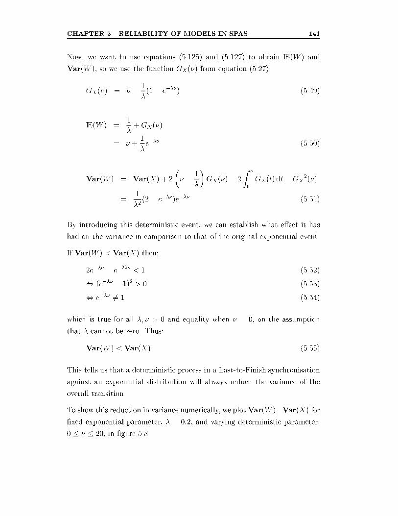
CHAPTER 5. RELIABILITY OF MODELS IN SPAS 141
Now, we want to use equations (5.125) and (5.127) to obtain IE(W ) and
Var(W ), so we use the function GX(�) from equation (5.27):
GX(�) = � � 1
�(1� e���) (5.49)
IE(W ) =1
�+GX(�)
= � +1
�e��� (5.50)
Var(W ) = Var(X) + 2
�� � 1
�
�GX(�)� 2
Z �
0
GX(t) dt�GX2(�)
=1
�2(2� e���)e��� (5.51)
By introducing this deterministic event, we can establish what e�ect it has
had on the variance in comparison to that of the original exponential event.
If Var(W ) < Var(X) then:
2e��� � e�2�� < 1 (5.52)
, (e��� � 1)2 > 0 (5.53)
, e��� 6= 1 (5.54)
which is true for all �; � > 0 and equality when � = 0, on the assumption
that � cannot be zero. Thus:
Var(W ) < Var(X) (5.55)
This tells us that a deterministic process in a Last-to-Finish synchronisation
against an exponential distribution will always reduce the variance of the
overall transition.
To show this reduction in variance numerically, we plotVar(W )�Var(X) for
�xed exponential parameter, � = 0:2, and varying deterministic parameter,
0 � � � 20, in �gure 5.8.
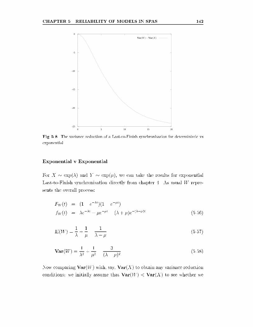
CHAPTER 5. RELIABILITY OF MODELS IN SPAS 142
-25
-20
-15
-10
-5
0
0 5 10 15 20
Fig. 5.8. The variance reduction of a Last-to-Finish synchronisation for deterministic vs
exponential.
Exponential v Exponential
For X � exp(�) and Y � exp(�), we can take the results for exponential
Last-to-Finish synchronisation directly from chapter 4. As usual W repre-
sents the overall process:
FW (t) = (1� e��t)(1� e��t)fW (t) = �e��t + �e��t � (�+ �)e�(�+�)t (5.56)
IE(W ) =1
�+
1
�� 1
�+ �(5.57)
Var(W ) =1
�2+
1
�2� 3
(�+ �)2(5.58)
Now comparing Var(W ) with, say, Var(X) to obtain any variance reduction
conditions: we initially assume that Var(W ) < Var(X) to see whether we
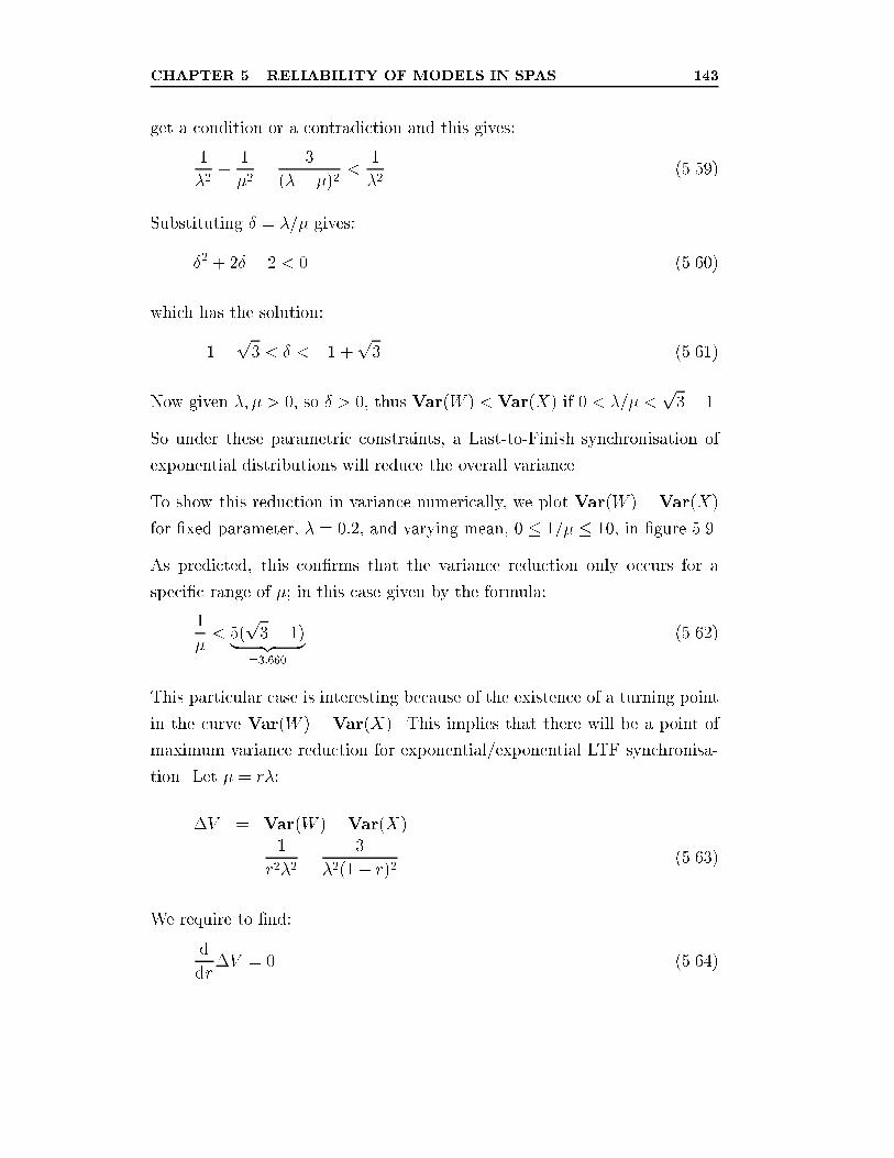
CHAPTER 5. RELIABILITY OF MODELS IN SPAS 143
get a condition or a contradiction and this gives:
1
�2+
1
�2� 3
(�+ �)2<
1
�2(5.59)
Substituting � = �=� gives:
�2 + 2� � 2 < 0 (5.60)
which has the solution:
�1�p3 < � < �1 +
p3 (5.61)
Now given �; � > 0, so � > 0, thus Var(W ) < Var(X) if 0 < �=� <p3� 1.
So under these parametric constraints, a Last-to-Finish synchronisation of
exponential distributions will reduce the overall variance.
To show this reduction in variance numerically, we plot Var(W )�Var(X)
for �xed parameter, � = 0:2, and varying mean, 0 � 1=� � 10, in �gure 5.9.
As predicted, this con�rms that the variance reduction only occurs for a
speci�c range of �; in this case given by the formula:
1
�< 5(p3� 1)| {z }
=3:660
(5.62)
This particular case is interesting because of the existence of a turning point
in the curve Var(W ) �Var(X). This implies that there will be a point of
maximum variance reduction for exponential/exponential LTF synchronisa-
tion. Let � = r�:
�V = Var(W )�Var(X)
=1
r2�2� 3
�2(1 + r)2(5.63)
We require to �nd:
d
dr�V = 0 (5.64)
CHAPTER 5. RELIABILITY OF MODELS IN SPAS 144
-10
0
10
20
30
40
50
60
70
0 1 2 3 4 5 6 7 8 9 10
Fig. 5.9. The variance reduction of a Last-to-Finish synchronisation for exponential vs
exponential.
which gives the following cubic:
2r3 � 3r2 � 3r � 1 = 0 (5.65)
and gives the only real solution r = 2:2611667.
Again, this result concurs with �gure 5.9 where we can see that the point of
maximum variance reduction occurs at 1=� = (0:2� 2:2611667)�1 = 2:211.
Uniform v Deterministic
Let X � U [a; b] where a = � � � and b = � + � and Y � �(�). As before,
for simplicity we would like to make use of the results of equations (5.125)
and (5.127). To do so we require GX(t); the calculations are slightly more in-
volved for the multiple cases of the uniform distribution, so again we will state
the results without intermediate steps in this section. From equation (5.37):
GX(t) =
8><>:
0 t < a
(t� a)2=4� a � t < b
t� � b � t
(5.66)
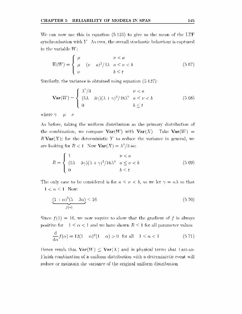
CHAPTER 5. RELIABILITY OF MODELS IN SPAS 145
We can now use this in equation (5.125) to give us the mean of the LTF
synchronisation with Y . As ever, the overall stochastic behaviour is captured
in the variable W :
IE(W ) =
8><>:
� � < a
�+ (� � a)2=4� a � � < b
� b � t
(5.67)
Similarly, the variance is obtained using equation (5.127):
Var(W ) =
8><>:
�2=3 � < a
(5�� 3 )(�+ )3=48�2 a � � < b
0 b � t
(5.68)
where = �� �.As before, taking the uniform distribution as the primary distribution of
the combination, we compare Var(W ) with Var(X). Take Var(W ) =
RVar(X); for the deterministic Y to reduce the variance in general, we
are looking for R < 1. Now Var(X) = �2=3 so:
R =
8><>:
1 � < a
(5�� 3 )(�+ )3=16�4 a � � < b
0 b � t
(5.69)
The only case to be considered is for a � � < b, so we let = �� so that
�1 < � � 1. Now:
(1 + �)3(5� 3�)| {z }f(�)
� 16 (5.70)
Since f(1) = 16, we now require to show that the gradient of f is always
positive for �1 � � < 1 and we have shown R � 1 for all parameter values.
d
d�f(�) = 12(1 + �)2(1� �) > 0 for all �1 � � < 1 (5.71)
Hence result that Var(W ) � Var(X) and in physical terms that Last-to-
Finish combination of a uniform distribution with a deterministic event will
reduce or maintain the variance of the original uniform distribution.
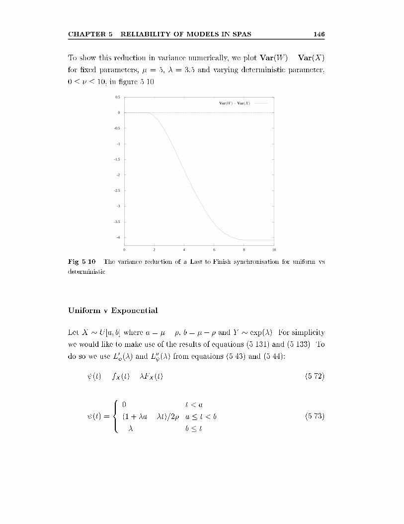
CHAPTER 5. RELIABILITY OF MODELS IN SPAS 146
To show this reduction in variance numerically, we plot Var(W )�Var(X)
for �xed parameters, � = 5, � = 3:5 and varying deterministic parameter,
0 � � � 10, in �gure 5.10.
-4
-3.5
-3
-2.5
-2
-1.5
-1
-0.5
0
0.5
0 2 4 6 8 10
Fig. 5.10. The variance reduction of a Last-to-Finish synchronisation for uniform vs
deterministic.
Uniform v Exponential
Let X � U [a; b] where a = �� �, b = �+ � and Y � exp(�). For simplicity
we would like to make use of the results of equations (5.131) and (5.133). To
do so we use L0 (�) and L00 (�) from equations (5.43) and (5.44):
(t) = fX(t)� �FX(t) (5.72)
(t) =
8><>:
0 t < a
(1 + �a� �t)=2� a � t < b
�� b � t
(5.73)
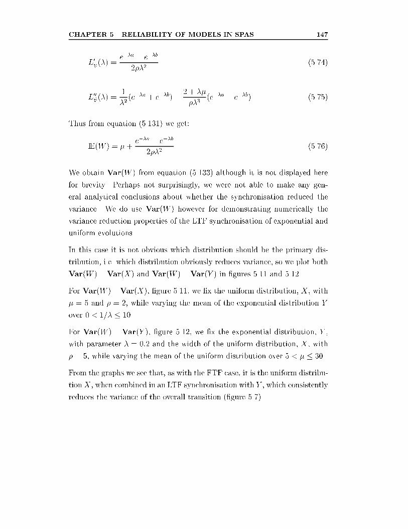
CHAPTER 5. RELIABILITY OF MODELS IN SPAS 147
L0 (�) =e��a � e��b
2��2(5.74)
L00 (�) =1
�2(e��a + e��b)� 2 + ��
��3(e��a � e��b) (5.75)
Thus from equation (5.131) we get:
IE(W ) = �+e��a � e��b
2��2(5.76)
We obtain Var(W ) from equation (5.133) although it is not displayed here
for brevity. Perhaps not surprisingly, we were not able to make any gen-
eral analytical conclusions about whether the synchronisation reduced the
variance. We do use Var(W ) however for demonstrating numerically the
variance reduction properties of the LTF synchronisation of exponential and
uniform evolutions.
In this case it is not obvious which distribution should be the primary dis-
tribution, i.e. which distribution obviously reduces variance, so we plot both
Var(W )�Var(X) and Var(W )�Var(Y ) in �gures 5.11 and 5.12.
For Var(W )�Var(X), �gure 5.11, we �x the uniform distribution, X, with
� = 5 and � = 2, while varying the mean of the exponential distribution Y
over 0 < 1=� � 10.
For Var(W ) �Var(Y ), �gure 5.12, we �x the exponential distribution, Y ,
with parameter � = 0:2 and the width of the uniform distribution, X, with
� = 5, while varying the mean of the uniform distribution over 5 < � � 30.
From the graphs we see that, as with the FTF case, it is the uniform distribu-
tionX, when combined in an LTF synchronisation with Y , which consistently
reduces the variance of the overall transition (�gure 5.7).
CHAPTER 5. RELIABILITY OF MODELS IN SPAS 148
-10
0
10
20
30
40
50
60
70
80
90
0 1 2 3 4 5 6 7 8 9 10
Fig. 5.11. The variance reduction of a Last-to-Finish synchronisation for exponential vs
uniform.
5.5 Worked Examples
5.5.1 Search Algorithm
As an example of how to improve the reliability of a system, we consider
a search algorithm. The goal is to design a second algorithm which, when
combined in a First-to-Finish strategy, would improve the reliability of the
overall search. In this case, we consider improved reliability to mean decreased
variance.
As an initial gambit we devise a na��ve algorithm for searching an array of
size N . We make the following assumptions about the search:
1. the data in the array is unordered
2. fetching any element from the array is achieved in constant time, �
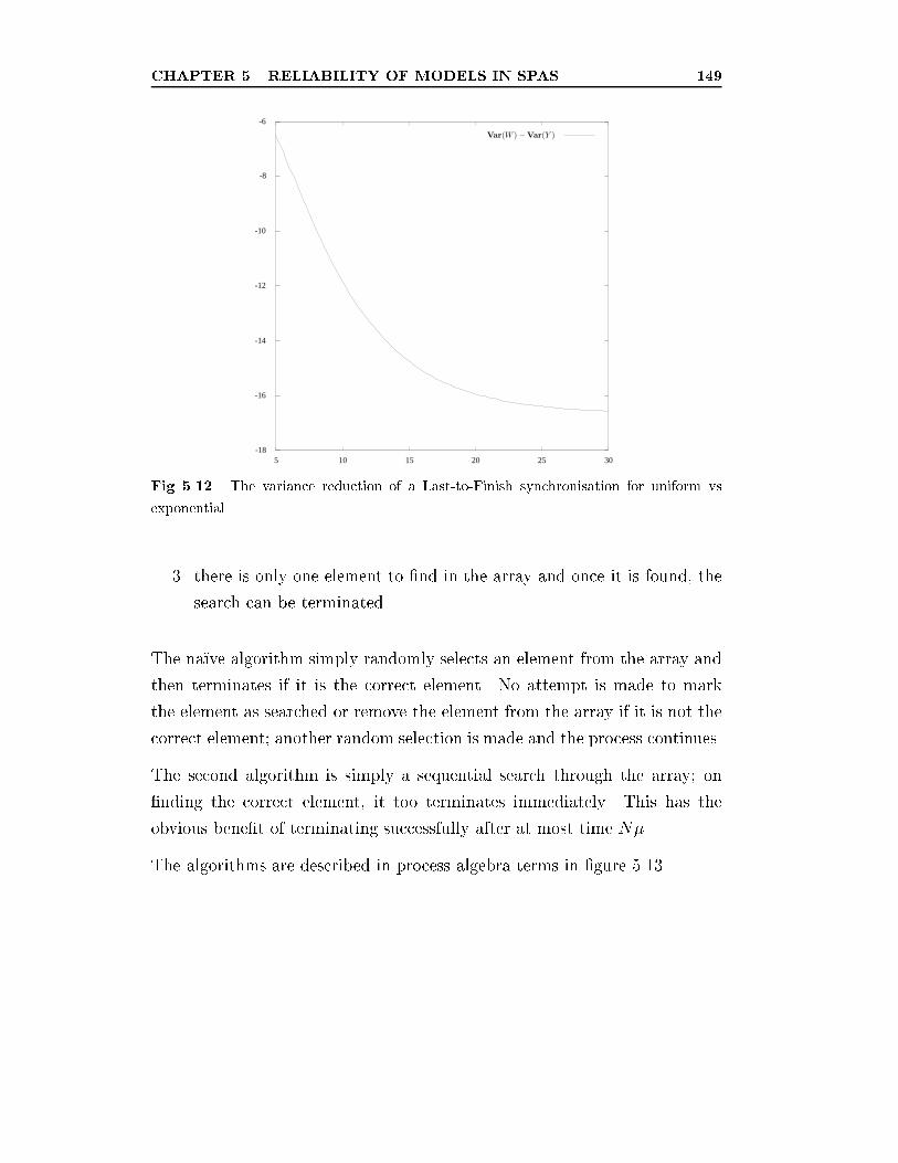
CHAPTER 5. RELIABILITY OF MODELS IN SPAS 149
-18
-16
-14
-12
-10
-8
-6
5 10 15 20 25 30
Fig. 5.12. The variance reduction of a Last-to-Finish synchronisation for uniform vs
exponential.
3. there is only one element to �nd in the array and once it is found, the
search can be terminated.
The na��ve algorithm simply randomly selects an element from the array and
then terminates if it is the correct element. No attempt is made to mark
the element as searched or remove the element from the array if it is not the
correct element; another random selection is made and the process continues.
The second algorithm is simply a sequential search through the array; on
�nding the correct element, it too terminates immediately. This has the
obvious bene�t of terminating successfully after at most time N�.
The algorithms are described in process algebra terms in �gure 5.13.
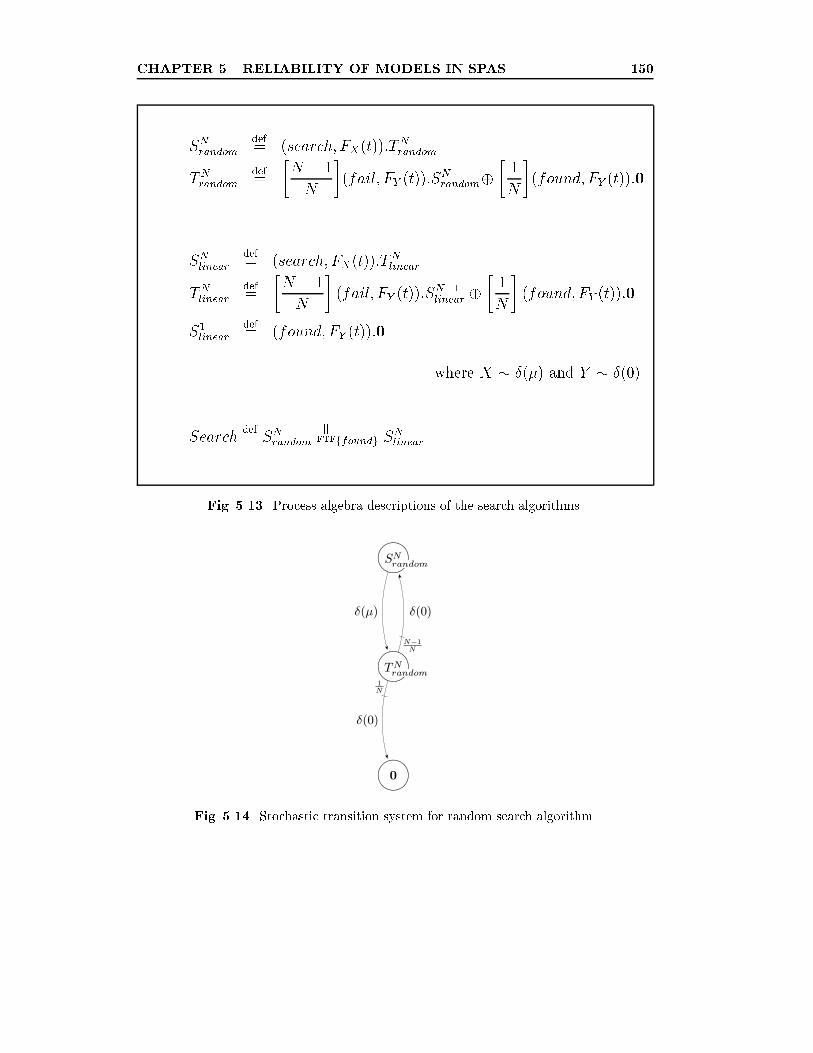
CHAPTER 5. RELIABILITY OF MODELS IN SPAS 150
SNrandomdef= (search; FX(t)):T
Nrandom
TNrandomdef=
�N � 1
N
�(fail; FY (t)):S
Nrandom�
�1
N
�(found; FY (t)):0
SNlineardef= (search; FX(t)):T
Nlinear
TNlineardef=
�N � 1
N
�(fail; FY (t)):S
N�1linear �
�1
N
�(found; FY (t)):0
S1linear
def= (found; FY (t)):0
where X � �(�) and Y � �(0)
Searchdef= SNrandom
kFTFffoundg S
Nlinear
Fig. 5.13. Process algebra descriptions of the search algorithms.
Fig. 5.14. Stochastic transition system for random search algorithm.
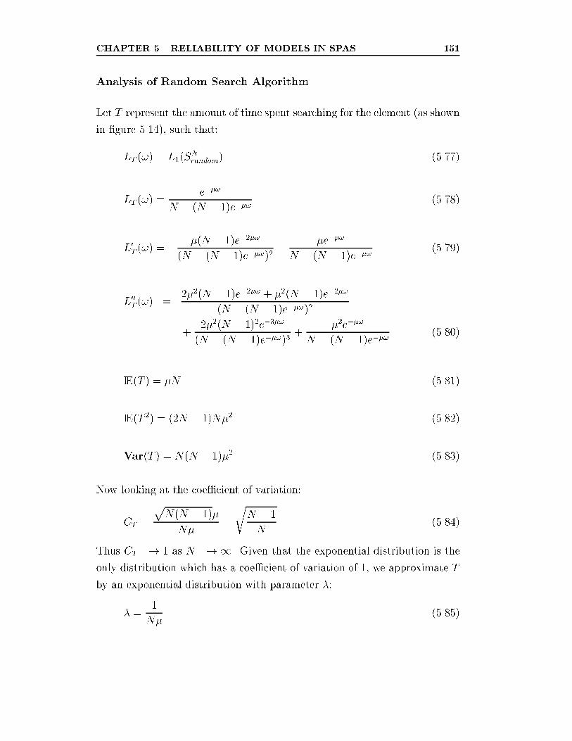
CHAPTER 5. RELIABILITY OF MODELS IN SPAS 151
Analysis of Random Search Algorithm
Let T represent the amount of time spent searching for the element (as shown
in �gure 5.14), such that:
LT (!) = L1(SNrandom) (5.77)
LT (!) =e��!
N � (N � 1)e��!(5.78)
L0T (!) = ��(N � 1)e�2�!
(N � (N � 1)e��!)2� �e��!
N � (N � 1)e��!(5.79)
L00T (!) =2�2(N � 1)e�2�! + �2(N � 1)e�2�!
(N � (N � 1)e��!)2
+2�2(N � 1)2e�3�!
(N � (N � 1)e��!)3+
�2e��!
N � (N � 1)e��!(5.80)
IE(T ) = �N (5.81)
IE(T 2) = (2N � 1)N�2 (5.82)
Var(T ) = N(N � 1)�2 (5.83)
Now looking at the coe�cient of variation:
CT =
pN(N � 1)�
N�=
rN � 1
N(5.84)
Thus CT �! 1 as N �! 1. Given that the exponential distribution is the
only distribution which has a coe�cient of variation of 1, we approximate T
by an exponential distribution with parameter �:
� =1
N�(5.85)
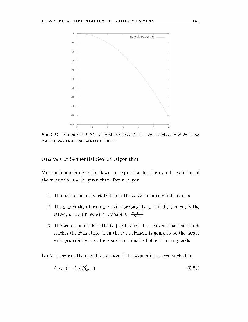
CHAPTER 5. RELIABILITY OF MODELS IN SPAS 152
-100
-90
-80
-70
-60
-50
-40
-30
-20
-10
0
0 1 2 3 4 5 6
Fig. 5.15. �V1 against IE(T 0) for �xed size array, N = 5: the introduction of the linear
search produces a large variance reduction.
Analysis of Sequential Search Algorithm
We can immediately write down an expression for the overall evolution of
the sequential search, given that after r stages:
1. The next element is fetched from the array, incurring a delay of �.
2. The search then terminates with probability 1N�r
if the element is the
target, or continues with probability N�r�1N�r
.
3. The search proceeds to the (r+1)th stage. In the event that the search
reaches the Nth stage, then the Nth element is going to be the target
with probability 1, so the search terminates before the array ends.
Let T 0 represent the overall evolution of the sequential search, such that:
LT 0(!) = L1(SNlinear) (5.86)
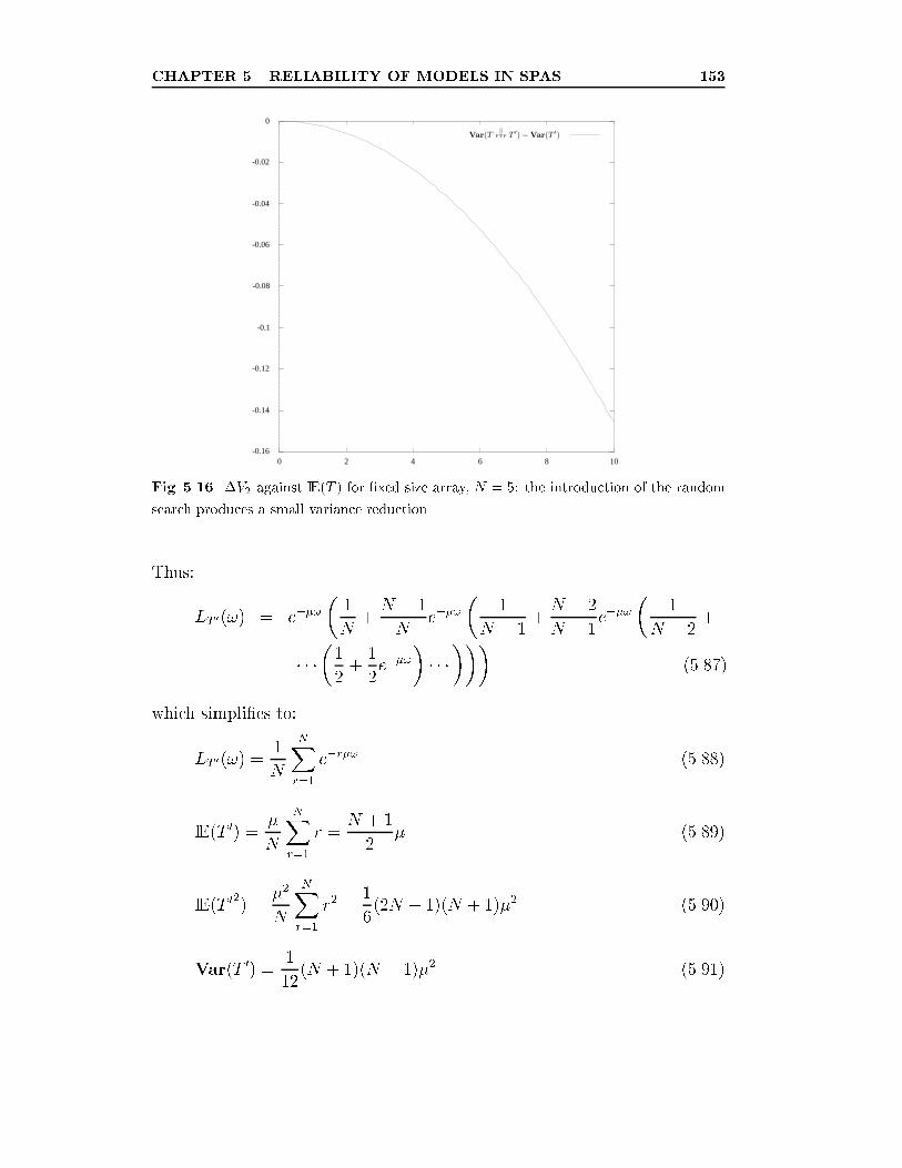
CHAPTER 5. RELIABILITY OF MODELS IN SPAS 153
-0.16
-0.14
-0.12
-0.1
-0.08
-0.06
-0.04
-0.02
0
0 2 4 6 8 10
Fig. 5.16. �V2 against IE(T ) for �xed size array, N = 5: the introduction of the random
search produces a small variance reduction.
Thus:
LT 0(!) = e��!�1
N+N � 1
Ne��!
�1
N � 1+N � 2
N � 1e��!
�1
N � 2+
� � ��1
2+1
2e��!
�� � ����
(5.87)
which simpli�es to:
LT 0(!) =1
N
NXr=1
e�r�! (5.88)
IE(T 0) =�
N
NXr=1
r =N + 1
2� (5.89)
IE(T 02) =�2
N
NXr=1
r2 =1
6(2N + 1)(N + 1)�2 (5.90)
Var(T 0) =1
12(N + 1)(N � 1)�2 (5.91)
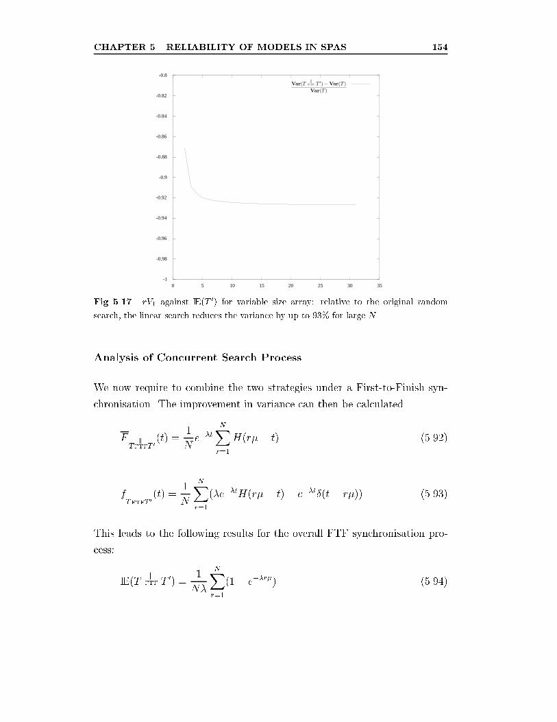
CHAPTER 5. RELIABILITY OF MODELS IN SPAS 154
-1
-0.98
-0.96
-0.94
-0.92
-0.9
-0.88
-0.86
-0.84
-0.82
-0.8
0 5 10 15 20 25 30 35
Fig. 5.17. rV1 against IE(T 0) for variable size array: relative to the original random
search, the linear search reduces the variance by up to 93% for large N .
Analysis of Concurrent Search Process
We now require to combine the two strategies under a First-to-Finish syn-
chronisation. The improvement in variance can then be calculated.
FT
kFTFT 0
(t) =1
Ne��t
NXr=1
H(r�� t) (5.92)
fT
kFTFT 0
(t) =1
N
NXr=1
(�e��tH(r�� t) + e��t�(t� r�)) (5.93)
This leads to the following results for the overall FTF synchronisation pro-
cess:
IE(Tk
FTF T 0) =1
N�
NXr=1
(1� e��r�) (5.94)
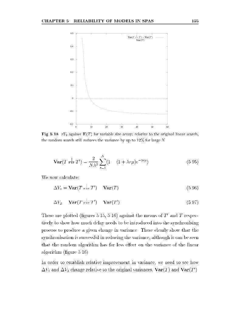
CHAPTER 5. RELIABILITY OF MODELS IN SPAS 155
-0.2
-0.1
0
0.1
0.2
0.3
0.4
0.5
0 10 20 30 40 50 60
Fig. 5.18. rV2 against IE(T ) for variable size array: relative to the original linear search,
the random search still reduces the variance by up to 12% for large N .
Var(Tk
FTF T 0) =2
N�2
NXr=1
(1� (1 + �r�)e��r�) (5.95)
We now calculate:
�V1 = Var(Tk
FTF T 0)�Var(T ) (5.96)
�V2 = Var(Tk
FTF T 0)�Var(T 0) (5.97)
These are plotted (�gures 5.15, 5.16) against the means of T 0 and T respec-
tively to show how much delay needs to be introduced into the synchronising
process to produce a given change in variance. These clearly show that the
synchronisation is successful in reducing the variance, although it can be seen
that the random algorithm has far less e�ect on the variance of the linear
algorithm (�gure 5.16).
In order to establish relative improvement in variance, we need to see how
�V1 and �V2 change relative to the original variances, Var(T ) and Var(T0).
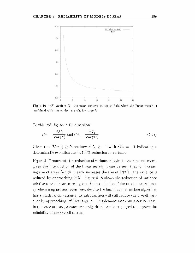
CHAPTER 5. RELIABILITY OF MODELS IN SPAS 156
-0.65
-0.6
-0.55
-0.5
-0.45
-0.4
-0.35
0 5 10 15 20 25 30
Fig. 5.19. rE1 against N : the mean reduces by up to 62% when the linear search is
combined with the random search, for large N .
To this end, �gures 5.17, 5.18 show:
rV1 =�V1
Var(T )and rV2 =
�V2Var(T 0)
(5.98)
Given that Var(�) � 0, we have rVN � �1 with rVN = �1 indicating a
deterministic evolution and a 100% reduction in variance.
Figure 5.17 represents the reduction of variance relative to the random search,
given the introduction of the linear search; it can be seen that for increas-
ing size of array (which linearly increases the size of IE(T 0)), the variance is
reduced by approaching 93%. Figure 5.18 shows the reduction of variance
relative to the linear search, given the introduction of the random search as a
synchronising process; even here, despite the fact that the random algorithm
has a much larger variance, its introduction will still reduce the overall vari-
ance by approaching 12% for large N . This demonstrates our assertion that,
in this case at least, a concurrent algorithm can be employed to improve the
reliability of the overall system.
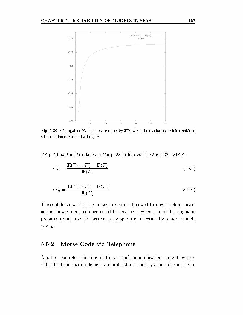
CHAPTER 5. RELIABILITY OF MODELS IN SPAS 157
-0.38
-0.36
-0.34
-0.32
-0.3
-0.28
-0.26
0 5 10 15 20 25 30
Fig. 5.20. rE2 against N : the mean reduces by 27% when the random search is combined
with the linear search, for large N .
We produce similar relative mean plots in �gures 5.19 and 5.20, where:
rE1 =IE(T
kFTF T 0)� IE(T )
IE(T )(5.99)
rE2 =IE(T
kFTF T 0)� IE(T 0)
IE(T 0)(5.100)
These plots show that the means are reduced as well through such an inter-
action, however an instance could be envisaged when a modeller might be
prepared to put up with larger average operation in return for a more reliable
system.
5.5.2 Morse Code via Telephone
Another example, this time in the area of communications, might be pro-
vided by trying to implement a simple Morse code system using a ringing
CHAPTER 5. RELIABILITY OF MODELS IN SPAS 158
telephone|the idea being that the phone is never answered and the infor-
mation is conveyed only by the length of time it rings. There is inherent
uncertainty in this problem, as the person or protocol doing the ringing can
have no idea whether the phone at the other end is actually ringing or im-
portantly how long it has been ringing for.
Although this source of error could be mitigated by error-correcting codes,
the e�ciency of the overall protocol could be substantially improved if the
underlying transport mechanism has a smaller chance of error.
System Description
To describe such a process, we need two parallel processes to represent the
calling process (R in �gure 5.21) and the network connecting process (C in
�gure 5.21). Thus ring taking random time X represents the amount of
time that the protocol spends waiting after dialling the number; this can be
varied according to whether the protocol is dialling a dot or a dash. The
connect action, taking time Y , is enabled simultaneously with the ring event
and represents the amount of time the network takes to connect the call,
and thus the amount of time before the receiving phone starts to ring. The
stochastic transition system for the protocol is shown in �gure 5.22.
As can be seen from �gure 5.22, we use the fact that we are working with
a pre-emptive resume strategy to give us the key transition2 (XjY < X) (Y jY < X). This is the residual time left by the ring action after it was pre-
empted by the connect action and therefore, crucially, represents the time
that the phone actually rings at the receiver's end.
2For some formulations of this problem, we discovered that we cannot obtain a well-
de�ned independent distribution representing the residual (X jY < X) process. Further
research is needed to understand when the operator can be used legitimately.
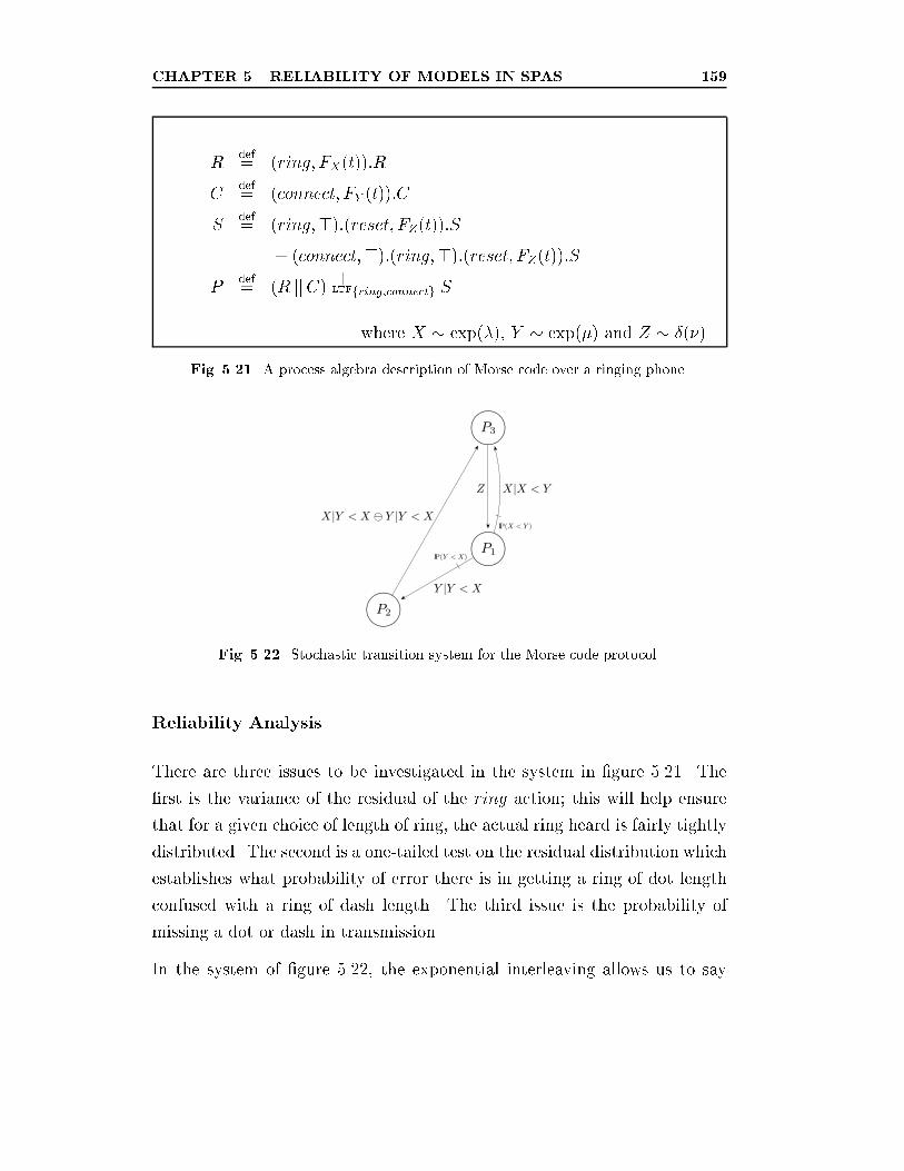
CHAPTER 5. RELIABILITY OF MODELS IN SPAS 159
Rdef= (ring; FX(t)):R
Cdef= (connect; FY (t)):C
Sdef= (ring;>):(reset; FZ(t)):S
+ (connect;>):(ring;>):(reset; FZ(t)):SP
def= (R jjC) k
LTFfring;connectg S
where X � exp(�), Y � exp(�) and Z � �(�)
Fig. 5.21. A process algebra description of Morse code over a ringing phone.
Fig. 5.22. Stochastic transition system for the Morse code protocol.
Reliability Analysis
There are three issues to be investigated in the system in �gure 5.21. The
�rst is the variance of the residual of the ring action; this will help ensure
that for a given choice of length of ring, the actual ring heard is fairly tightly
distributed. The second is a one-tailed test on the residual distribution which
establishes what probability of error there is in getting a ring of dot length
confused with a ring of dash length. The third issue is the probability of
missing a dot or dash in transmission.
In the system of �gure 5.22, the exponential interleaving allows us to say
CHAPTER 5. RELIABILITY OF MODELS IN SPAS 160
without calculation that (XjY < X) (Y jY < X) � exp(�). Thus the
variance of the residual is simply 1=�2. This is really only an indication
and tells us that, for small values of �, there might well be a possibility of
confusion of a dash with a dot, but not vice-versa.
In actual fact we have two types of system, one for which a dot is being
transmitted where X = X1 � exp(�1) and one for which a dash is being
transmitted, X = X2 � exp(�2). If we set �1 = k� for a dot, �2 = k�=2 for
a dash and the threshold for deciding which is which at the receiving end as
, then we see that:
IP(dot is not sent) = p1 = IP(X1 < Y ) =k
k + 1(5.101)
IP(dash is not sent) = p2 = IP(X2 < Y ) =k
k + 2(5.102)
IP(dot is misreceived as a dash) = p3 = FX1( ) = e�k � (5.103)
IP(dash is misreceived as a dot) = p4 = FX2( ) = 1� e�k �=2 (5.104)
Now for simplicity in the error-correcting coding layer that would sit above
this protocol, it would be desirable for the transmission error probabilities to
be the same, i.e. p3 = p4. Thus:
e�k � = 1� e�k �=2 (5.105)
giving:
e�k �=2 =
p5� 1
2(5.106)
=2
k�ln
�2p5� 1
�(5.107)
So:
IP(transmission error) =3�p5
2= 0:382 (5.108)
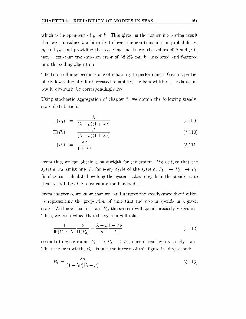
CHAPTER 5. RELIABILITY OF MODELS IN SPAS 161
which is independent of � or k. This gives us the rather interesting result
that we can reduce k arbitrarily to lower the non-transmission probabilities,
p1 and p2, and providing the receiving end knows the values of k and � in
use, a constant transmission error of 38.2% can be predicted and factored
into the coding algorithm.
The trade-o� now becomes one of reliability to performance. Given a partic-
ularly low value of k for increased reliability, the bandwidth of the data link
would obviously be correspondingly low.
Using stochastic aggregation of chapter 3, we obtain the following steady-
state distribution:
�(P1) =�
(�+ �)(1 + ��)(5.109)
�(P2) =�
(�+ �)(1 + ��)(5.110)
�(P3) =��
1 + ��(5.111)
From this, we can obtain a bandwidth for the system. We deduce that the
system transmits one bit for every cycle of the system, P1 �! P2 �! P3.
So if we can calculate how long the system takes to cycle in the steady-state
then we will be able to calculate the bandwidth.
From chapter 3, we know that we can interpret the steady-state distribution
as representing the proportion of time that the system spends in a given
state. We know that in state P3, the system will spend precisely � seconds.
Thus, we can deduce that the system will take:
1
IP(Y < X)
�
�(P3)=�+ �
�
1 + ��
�(5.112)
seconds to cycle round P1 �! P2 �! P3, once it reaches its steady-state.
Thus the bandwidth, BP , is just the inverse of this �gure in bits/second:
BP =��
(1 + ��)(�+ �)(5.113)
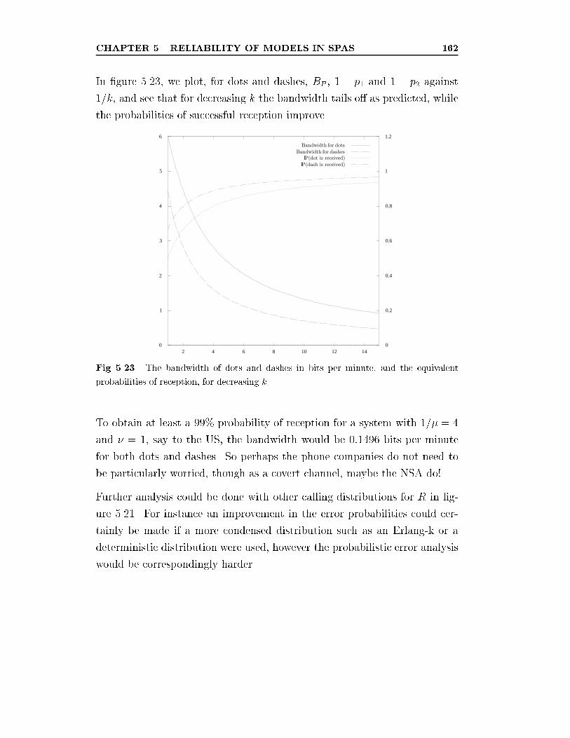
CHAPTER 5. RELIABILITY OF MODELS IN SPAS 162
In �gure 5.23, we plot, for dots and dashes, BP , 1 � p1 and 1 � p2 against1=k, and see that for decreasing k the bandwidth tails o� as predicted, while
the probabilities of successful reception improve.
0
0.2
0.4
0.6
0.8
1
1.2
0
1
2
3
4
5
6
2 4 6 8 10 12 14
Fig. 5.23. The bandwidth of dots and dashes in bits per minute, and the equivalent
probabilities of reception, for decreasing k.
To obtain at least a 99% probability of reception for a system with 1=� = 4
and � = 1, say to the US, the bandwidth would be 0:1496 bits per minute
for both dots and dashes. So perhaps the phone companies do not need to
be particularly worried, though as a covert channel, maybe the NSA do!
Further analysis could be done with other calling distributions for R in �g-
ure 5.21. For instance an improvement in the error probabilities could cer-
tainly be made if a more condensed distribution such as an Erlang-k or a
deterministic distribution were used, however the probabilistic error analysis
would be correspondingly harder.
CHAPTER 5. RELIABILITY OF MODELS IN SPAS 163
5.6 Conclusion
In this chapter, we have discussed the di�erence between average behaviour or
performance and variant behaviour or reliability. Performance in stochastic
systems is usually obtained from stationary distributions and represents long-
run state probabilities. As such, it automatically discounts variation or short-
term extreme behaviour.
What has been attempted here, therefore, is to show that by identifying a key
transition or set of transitions, and by employing techniques to reduce the
variance of such a transition, the reliability (i.e. determinism) of the whole
system can be improved.
5.6.1 Equivalences for Model Checking
In summarising this chapter, we are keen to demonstrate how such a set of
properties can be used to extend reliability analysis systematically and not
necessarily just on a system by system basis.
Traditionally in process algebras this is achieved by constructing a bisimilar-
ity, a relation that allies two processes. Such a relationship, once formally
stated, can be systematically tested for and used at di�erent levels of the
system design process. Two models might display the same properties (if
one is looking to replace the other), or a model and a speci�cation (used
for model re�nement and invariant proof) or even design and speci�cation
(checking compliance to a formal standard perhaps).
Unfortunately we are in a dilemma, since although we have shown what
reliability might mean in a stochastic setting, our examples demonstrate
that it can be quite a model speci�c attribute. In what way model speci�c?
Insofar as the modeller needs to know which parts of the model are reliability
critical and for which parts it is not so important.
This is at once an advantage and a disadvantage. Computationally, we have
seen that reliability need not necessarily be anything like as hard a quantity
CHAPTER 5. RELIABILITY OF MODELS IN SPAS 164
to calculate as, say, a steady-state distribution. This is lucky since general
steady-state distribution solutions of generally-distributed systems are an-
alytically beyond the current state-of-the-art. Reliability tends to be path
speci�c and need not necessarily involve consideration of the whole system.
Depending on how the system has been constructed in a process algebra, the
reliability of a key part of the model may only involve a few local transitions.
This brings us to the disadvantage however, the fact that reliability analysis
still requires quite a well informed modeller. The construction of the model is
the �rst hurdle, and if done at too high a level of detail or looking at the wrong
communication model abstraction, can make analysis prohibitively hard. Our
experience with constructing the telephone example tells us that if the wrong
type of model is constructed then reliability analysis can be almost as hard as
steady-state analysis. Further, a fundamental understanding of the process
is required to understand which parts of the system are reliability critical.
This latter point is not necessarily a drawback though, since modelling is,
after all, carried out to understand a system's operation better. Experience
will clearly be needed at the modelling level.
We postulate the existence of some equivalences or bisimulations of generally-
distributed models which might be of use. At the performance level, Larsen
and Skou's probabilistic bisimulation [73] considered probabilistic ux through
a Markovian process algebra; this clearly does not have a direct extension
to a generally-distributed environment. However the intention is to equate
systems which have the same long-term behaviour, so we might suggest a
performance equivalence which equates generally-distributed systems with
the same steady-state distribution. To allow model re�nement and speci�-
cation checking, we could allow systems to be stochastically aggregated into
a form where they might be checked.
On the reliability side, we suggest two path reliability equivalences which
operate at the local level, identi�ed earlier. The �rst would be to equate
paths of a system which have the same stochastic aggregation, that is that
their aggregated passage time is the same. Finally, a weaker path equivalence
CHAPTER 5. RELIABILITY OF MODELS IN SPAS 165
would be to equate paths with the same mean and variance. On a similar
basis, a reliability preorder could be established between paths which have
the same mean but di�ering variance; the smaller the variance the more
reliable the critical path.
These tools could then be applied to the relevant parts of a stochastically
speci�ed model to test for reliability constraints. Clearly more work is re-
quired to make these �rst attempts at generalising stochastic reliability more
concrete.
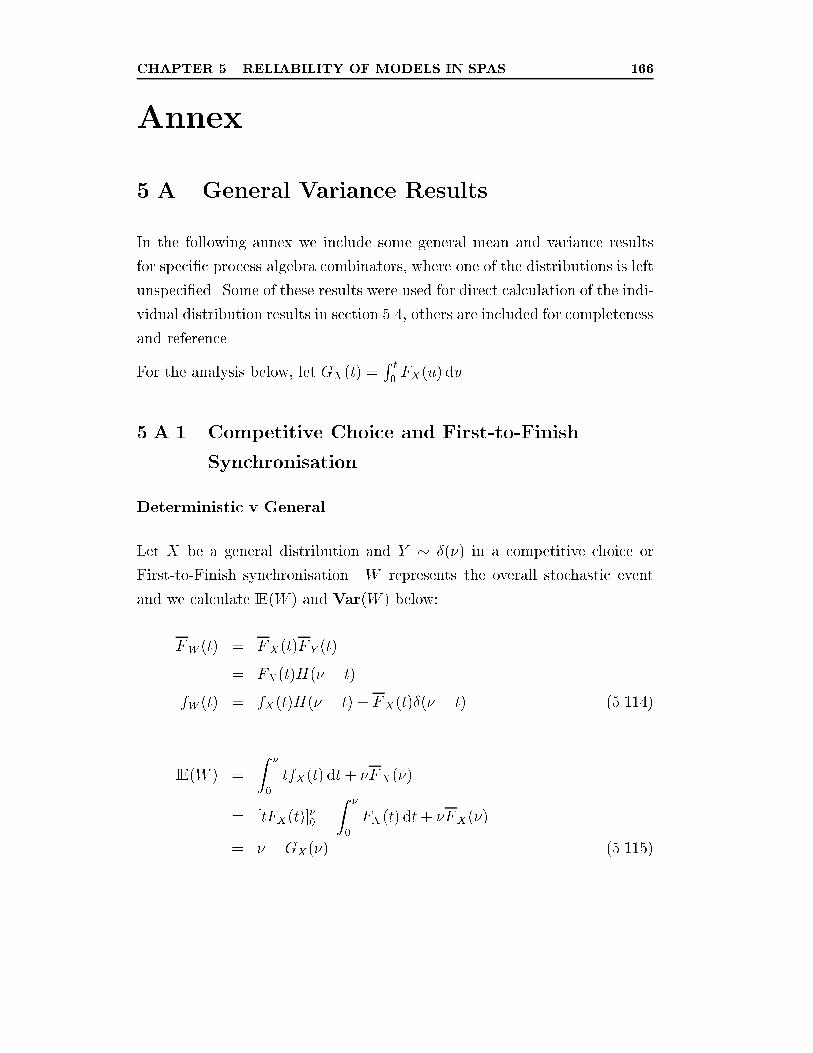
CHAPTER 5. RELIABILITY OF MODELS IN SPAS 166
Annex
5.A General Variance Results
In the following annex we include some general mean and variance results
for speci�c process algebra combinators, where one of the distributions is left
unspeci�ed. Some of these results were used for direct calculation of the indi-
vidual distribution results in section 5.4, others are included for completeness
and reference.
For the analysis below, let GX(t) =R t0FX(u) du.
5.A.1 Competitive Choice and First-to-Finish
Synchronisation
Deterministic v General
Let X be a general distribution and Y � �(�) in a competitive choice or
First-to-Finish synchronisation. W represents the overall stochastic event
and we calculate IE(W ) and Var(W ) below:
FW (t) = FX(t)F Y (t)
= FX(t)H(� � t)fW (t) = fX(t)H(� � t) + FX(t)�(� � t) (5.114)
IE(W ) =
Z �
0
tfX(t) dt+ �FX(�)
= [tFX(t)]�0 �
Z �
0
FX(t) dt+ �FX(�)
= � �GX(�) (5.115)
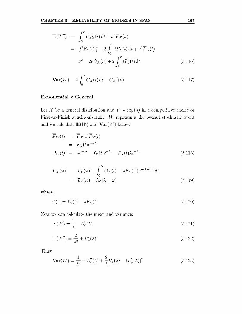
CHAPTER 5. RELIABILITY OF MODELS IN SPAS 167
IE(W 2) =
Z �
0
t2fX(t) dt+ �2FX(�)
= [t2FX(t)]�0 � 2
Z �
0
tFX(t) dt+ �2FX(t)
= �2 � 2�GX(�) + 2
Z �
0
GX(t) dt (5.116)
Var(W ) = 2
Z �
0
GX(t) dt�GX2(�) (5.117)
Exponential v General
Let X be a general distribution and Y � exp(�) in a competitive choice or
First-to-Finish synchronisation. W represents the overall stochastic event
and we calculate IE(W ) and Var(W ) below:
FW (t) = FX(t)F Y (t)
= FX(t)e��t
fW (t) = �e��t + fX(t)e��t � FX(t)�e��t (5.118)
LW (!) = LY (!) +
Z 1
0
(fX(t)� �FX(t))e�(�+!)t dt= LY (!) + L (�+ !) (5.119)
where:
(t) = fX(t)� �FX(t) (5.120)
Now we can calculate the mean and variance:
IE(W ) =1
�� L0 (�) (5.121)
IE(W 2) =2
�2+ L00 (�) (5.122)
Thus:
Var(W ) =1
�2+ L00 (�) +
2
�L0 (�)� (L0 (�))
2 (5.123)
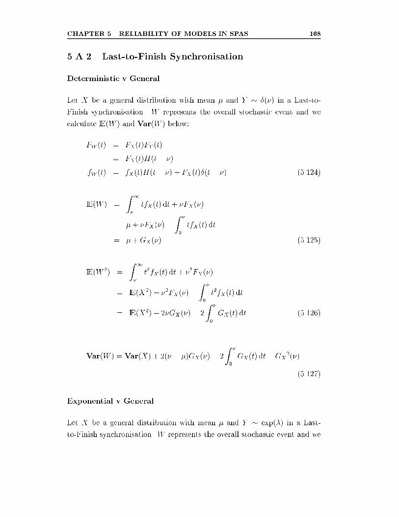
CHAPTER 5. RELIABILITY OF MODELS IN SPAS 168
5.A.2 Last-to-Finish Synchronisation
Deterministic v General
Let X be a general distribution with mean � and Y � �(�) in a Last-to-
Finish synchronisation. W represents the overall stochastic event and we
calculate IE(W ) and Var(W ) below:
FW (t) = FX(t)FY (t)
= FX(t)H(t� �)fW (t) = fX(t)H(t� �) + FX(t)�(t� �) (5.124)
IE(W ) =
Z 1
�
tfX(t) dt + �FX(�)
= �+ �FX(�)�Z �
0
tfX(t) dt
= �+GX(�) (5.125)
IE(W 2) =
Z 1
�
t2fX(t) dt+ �2FX(�)
= IE(X2) + �2FX(�)�Z �
0
t2fX(t) dt
= IE(X2) + 2�GX(�)� 2
Z �
0
GX(t) dt (5.126)
Var(W ) = Var(X) + 2(� � �)GX(�)� 2
Z �
0
GX(t) dt�GX2(�)
(5.127)
Exponential v General
Let X be a general distribution with mean � and Y � exp(�) in a Last-
to-Finish synchronisation. W represents the overall stochastic event and we
CHAPTER 5. RELIABILITY OF MODELS IN SPAS 169
calculate IE(W ) and Var(W ) below:
FW (t) = FX(t)FY (t)
= FX(t)(1� e��t)fW (t) = fX(t)(1� e��t) + FX(t)�e
��t (5.128)
LW (!) = �Z 1
0
(fX(t)� �FX(t))e�(�+!)t dt +Z 1
0
fX(t)e�!t dt
= LX(!)� L (�+ !) (5.129)
where:
(t) = fX(t)� �FX(t) (5.130)
Now we can calculate the mean and variance:
IE(W ) = IE(X) + L0 (�) (5.131)
IE(W 2) = IE(X2)� L00 (�) (5.132)
Thus:
Var(W ) = Var(X)� L00 (�)� 2IE(X)L0 (�)� (L0 (�))2 (5.133)
5.B Minimum and Maximum Distributions
of Random Variables
We want to demonstrate that the conditional expansion of the maximum and
minimum distributions as described by competitive choice, First-to-Finish
synchronisations and Last-to-Finish synchronisations (in section 5.3 and used
in derivations in �gures 5.1 and 5.2) are identical to the cumulative distribu-
tion function versions used in chapter 4 (equations (4.2) and (4.6)).
CHAPTER 5. RELIABILITY OF MODELS IN SPAS 170
5.B.1 Maximum Distribution
The maximum distribution is used for Last-to-Finish synchronisation. We
claim that for a random variable W = max(X; Y ):
FW (t) = IP(X > Y )FXjX>Y (t) + IP(Y > X)FY jY >X(t)
= FX(t)FY (t) (5.134)
Thus:
FW (t) = IP(X > Y )FXjX>Y (t) + IP(Y > X)FY jY >X(t)
= IP(X � t; X > Y ) + IP(Y � t; Y > X)
=
Z t
0
FY (u)fX(u) + FX(u)fY (u) du
=
Z t
0
d
du[FX(u)FY (u)] du
= [FX(u)FY (u)]t0 (5.135)
Since FX(0)FY (0) = 0:
FW (t) = FX(t)FY (t) (5.136)
5.B.2 Minimum Distribution
The minimum distribution is used for both competitive choice and First-to-
Finish synchronisation. We claim that for a random variableW = min(X; Y )3:
FW (t) = IP(X < Y )FXjX<Y (t) + IP(Y < X)FY jY <X(t)
= 1� FX(t)F Y (t) (5.137)
3This repeats a result from chapter 3, equations (3.59){(3.60), displayed here for com-
pleteness and ease-of-reference.
CHAPTER 5. RELIABILITY OF MODELS IN SPAS 171
Thus:
FW (t) = IP(X < Y )FXjX<Y (t) + IP(Y < X)FY jY <X(t)
= IP(X � t; X < Y ) + IP(Y � t; Y < X)
=
Z t
0
F Y (u)fX(u) + FX(u)fY (u) du
=
Z t
0
� d
du
�FX(u)F Y (u)
�du
=��FX(u)F Y (u)
�t0
(5.138)
Since FX(0)F Y (0) = 1:
FW (t) = 1� FX(t)F Y (t) (5.139)
Chapter 6
Conclusions
6.1 Overview
In this thesis, we have examined reliable modelling in the context of stochastic
process algebras. This took the form of improved treatment of generally-
distributed stochastic processes, improved accuracy of performance measures
in Markovian process algebras, and �nally, reduced model variance for greater
predictability and determinism within systems.
6.2 Summary
6.2.1 Introduction and Motivation
In chapter 1, we set out our reasoning and motivation for considering time in
addition to functional operation. In modelling temporal behaviour, we reason
that we are observing the full behaviour of a system. Thus we are able to
make statements about the reliability of operation of the system which are
time dependent and not just functionality dependent.
172
CHAPTER 6. CONCLUSIONS 173
This train of reasoning is not a particularly new one, but in fact underpins
the development of all the timed and stochastic process algebras, introduced
in chapter 2. Here, we have two goals: to demonstrate the progressive re�ne-
ment of process algebras from the purely functional to the stochastic; and
also to show what stochastic process algebras are currently good at doing
and where their analytical shortcomings might lie.
We identify that for Markovian process algebras, the solution techniques are
well developed for obtaining steady-state solutions of large Markov processes.
However, as the distributions get more general, so the underlying techniques
become less capable of dealing with larger models. In all cases, though, our
main complaint was that the solution techniques concentrated on the average
behaviour of the steady-state solution and thus ignored any of the tail-end
behaviour which might cause problems such as network jitter.
We also noted that the two longest standing Markovian process algebras,
which have been studied and honed the most, make an approximation in a
key area of the process algebra model: that of synchronisation.
Thus, we develop our approach for the thesis: a dual strategy to aid the
development of reliable models. The �rst strand, to investigate methods
of analysing generally-distributed processes which maintain the integrity of
both the model and distribution. By this we mean, a method which does not
alter the model, as insensitivity analysis does, and does not discard tail-end
behaviour, as in steady-state analysis. This motivates our work in chapter 3,
in which we develop the technique of stochastic aggregation.
6.2.2 Synchronisation
Our second strand of attack was implemented in chapter 4, where we exam-
ine the issue of synchronisation in stochastic process algebras and the Marko-
vian process algebras, MTIPP and PEPA, in particular. In recognising that
generally-distributed analysis techniques are going to be a�ected by space
and time complexity issues, we would like to improve the reliability of the
CHAPTER 6. CONCLUSIONS 174
performance �gures that these two algebras were able to produce. We gain
an understanding of the di�erent approximations that MTIPP and PEPA
made in synchronisation and how they a�ected their respective performance
�gures.
Now we can use the advanced tools (such as PEPA Workbench [33] and
TIPPtool [46]) and solution techniques that exist in the Markovian area (such
as quasi-reversibility [40], and quasi-separability [93] and similar product-
form solutions). We can obtain e�cient solutions to a given model and,
crucially, still understand how reliable this solution is likely to be. We may
even be in a position to improve the accuracy of the technique by running
multiple model versions with some of the di�erent synchronisation strategies
suggested in chapter 4.
6.2.3 Reliability Modelling
Having developed the stochastic aggregation method of chapter 3, we were
keen to see what tail-end behaviour we could model, having kept the distri-
bution information intact. We quickly realised that one of the key areas of
reliable modelling is that of keeping the variance small over critical paths of
execution. We saw that, if modelling with too di�use a distribution, there
is a tendency to get a variance explosion problem; generated primarily when
using the sequential pre�x combinator in stochastic process algebras. Most
of the chapter is then dedicated to examining which combinators and which
distribution types are good at reducing variance. We illustrated the point
with a searching algorithm which had its variance considerably improved by
the use of an appropriate combination with another technique.
We �nished with the insight that reliable modelling and reliability in stochas-
tic systems is a very diverse and problem-speci�c entity: in the same way
that performance modelling talks about issues such as bandwidth, resource
utilisation and throughput. However, we envisage that progress will be best
made by formally expressing concepts such as variance reduction or tail-test
CHAPTER 6. CONCLUSIONS 175
invariants in bisimulations. Only when this has happened formally can we
systematically model with these reliability goals in mind. However, in the
end, it still requires the modeller to know what quantity is critically impor-
tant to the problem and how that might be best translated into a stochastic
test on an SPA model.
6.3 Speci�c Results
6.3.1 Stochastic Aggregation and Probabilistic
Semantics
In chapter 3, we show how stochastic aggregation can be used to solve some
generally-distributed processes for their steady-state distributions. We also
demonstrate how it can be used to solve CTMCs, through analysing Marko-
vian process algebra models, in a progressive fashion with a small saving
in complexity terms. Through an example, we suggest how stochastic ag-
gregation might be used to analyse systems in a component-wise fashion:
aggregating the behaviour of other system components into a single variable
delay for a particular component, and thus solving a structurally simpler
model.
We also presented a form of probabilistic operational semantics, which act
as a direct mapping on to the stochastic transition systems of chapter 3.
This allowed us to specify probabilistically two Markovian process algebras
(PEPA and MTIPP), whereas previously they had only been speci�ed using
the traditional functional operational semantics. We also de�ned a generally-
distributed, pre-emptive restart stochastic process algebra with two synchro-
nisation models, FTF and LTF (�gure 3.27).
CHAPTER 6. CONCLUSIONS 176
6.3.2 Synchronisation Classi�cation and Reliable
Markovian Modelling
Chapter 4 coined the ideas of First-to-Finish and Last-to-Finish synchroni-
sation. It demonstrated that FTF synchronisation could be implemented
precisely in Markovian process algebras whereas LTF could not. In approx-
imating LTF synchronisation, we showed that MTIPP was not consistent
in its relative prediction, whereas PEPA would tend to overestimate per-
formance �gures. We showed that, in fact, no Markovian process algebra
could consistently underestimate our performance metrics, but nonetheless
came up with a model, PEPA*, which was e�ective at usually underestimat-
ing performance. We were therefore able to suggest using both PEPA and
PEPA* to obtain a more reliable estimate for the synchronisation. We anal-
ysed a third synchronisation operator, the mean-preserving synchronisation,
which was essentially an approximate insensitive transition and came closest
to the true solution. Finally, we managed to restrict the parameter space of
the MTIPP synchronisation, so that it would emulate the mean-preserving
synchronisation.
6.3.3 Classi�cation of Variance Reducing Operators
and Distributions
In chapter 5, we identi�ed increasing variance as a problem that would make
systems unreliable and simulation meaningless. We take the view that, if
stochastic process algebra modelling is carried out at the design stage of a
project, then this variance explosion can be mitigated. To achieve this we
were able to provide an analysis of which distributions, and under which
combinators, would reduce variance. We also provided useful metrics for
measuring this variance reduction.
CHAPTER 6. CONCLUSIONS 177
6.4 Further Investigation
There are two main areas of investigation that we would like to explore
further: that of improved generally-distributed stochastic analysis, which
would allow representation of a wider class of processes; and also a more
systematic approach to reliability modelling.
6.4.1 Component Aggregation
We view as particularly interesting the development of the component aggre-
gation technique, demonstrated in chapter 3 and also [10]. The problem area
of stochastic modelling and analysis is that of pre-emptive resume systems.
While we were able to provide steady-state analysis of general pre-emptive
restart systems (section 3.3.1), we were also able to show exactly why an
interleaving expansion approach could not be used for pre-emptive resume
systems (section 3.3.2)1. If the process of component aggregation could be
re�ned to deal with cyclically dependent components then it might well be
possible to obtain analysis of generally-distributed pre-emptive resume sys-
tems which is currently not possible. The fact that this would be embodied in
a stochastic process algebra environment rather than say, a queueing system
environment, would also automatically give it greater applicability.
1We wonder whether the non-existence of a �nite interleaving for even the simplest of
interacting systems (a G/G/1/3 queue, for example) might not have wider consequences
outside of the �eld of stochastic modelling. Simulation of such interacting processes in-
evitably involves synchronising with the internal clock of the system that the simulation
is running on; this synchronisation would clearly make the state-space �nite again and
may well destroy the equivalence with the system being simulated. What consequences
does this have for simulation of a system which is completely constructed of such simple
interactions, for example neural simulations?
CHAPTER 6. CONCLUSIONS 178
6.4.2 Reliability through Feature Modelling
Given that issues of reliability are quite diverse and model-speci�c, we see
the progression of this area in the development of a reliability description
language. We see the presentation of desirable features and properties of a
model through a form of modal calculus, as presented by Gilmore [35, 36], as
a particularly interesting technique. This approach might well lead to a form
of temporal model checking which could be automated and incorporated into
a tool.
Another approach, maybe more expressive but correspondingly less system-
atic, involves testing stochastic properties of a model with small synchronis-
ing fragments of stochastic process algebra. These so-called stochastic process
algebra probes [27] would passively measure key properties (sequences of ob-
servable actions) and, through the analysis of the combined model-probe
system, it would be ascertained whether a property had been met or not.
Bibliography
[1] Ajmone Marsan, M., Balbo, G., and Conte, G. Performance
Models of Multiprocessor Systems. MIT Press Series in Computer Sys-
tems. The MIT Press, 1986.
[2] Ajmone Marsan, M., Bianco, A., Cimminiera, L., Sisto, R.,
and Valenzano, A. A LOTOS extension for the performance anal-
ysis of distributed systems. IEEE/ACM Transactions on Networking
2, 2 (April 1994), 151{165.
[3] Ajmone Marsan, M., and Chiola, G. On Petri nets with deter-
ministic and exponentially distributed �ring times. In APN'87, Ad-
vances in Petri Nets, Proceedings of the 7th European Workshop on
Applications and Theory of Petri Nets (Oxford, June 1987), G. Rozen-
berg, Ed., vol. 266 of Lecture Notes in Computer Science, Springer-
Verlag, pp. 132{145.
[4] Ajmone Marsan, M., Conte, G., and Balbo, G. A class of gen-
eralized stochastic Petri nets for the performance evaluation of multi-
processor systems. ACM Transactions on Computer Systems 2, 2 (May
1984), 93{122.
[5] Allen, A. O. Probability, Statistics and Queueing Theory with Com-
puter Science Applications, 2nd ed. Academic Press, 1990.
179
BIBLIOGRAPHY 180
[6] Baeten, J. C. M., and Bergstra, J. A. Real time process algebra.
Formal Aspects of Computing 3, 2 (April-June 1991), 142{188.
[7] Bergstra, J. A., and Klop, J. W. Algebra for communicating
processes with abstraction. Journal of Theoretical Computer Science
37, 1 (May 1985), 77{121.
[8] Bernardo, M. Theory and Application of Extended Markovian Pro-
cess Algebra. PhD thesis, Department of Computer Science, University
of Bologna, February 1999.
[9] Bernardo, M., and Gorrieri, R. Extended Markovian Process
Algebra. In CONCUR'96, Proceedings of the 7th International Con-
ference on Concurrency Theory (Pisa, August 1996), U. Montanari
and V. Sassone, Eds., vol. 1119 of Lecture Notes in Computer Science,
Springer-Verlag, pp. 315{330.
[10] Bohnenkamp, H. C., and Haverkort, B. R. Stochastic event
structures for the decomposition of stochastic process algebra models.
In Hillston and Silva [57], pp. 25{39.
[11] Bowman, H., Bryans, J. W., and Derrick, J. Analysis of a
multimedia stream using stochastic process algebras. In Priami [84],
pp. 51{69.
[12] Bradley, J. T., and Davies, N. J. An aggregation technique for
analysing some generally distributed stochastic processes. CSTR Tech-
nical Report CSTR{99{003, Department of Computer Science, Univer-
sity of Bristol, Bristol BS8 1UB, UK, March 1999.
[13] Bradley, J. T., and Davies, N. J. Measuring improved reliability
in stochastic systems. In UKPEW'99, Proceedings of the 15th Annual
UK Performance Engineering Workshop [14], pp. 121{130.
[14] Bradley, J. T., and Davies, N. J., Eds. Proceedings of the 15th
Annual UK Performance Engineering Workshop (Bristol, July 1999),
BIBLIOGRAPHY 181
CSTR Technical Report, Department of Computer Science, University
of Bristol, Research Press. CSTR{99{007, ISBN 0 9524027 8 5.
[15] Bradley, J. T., and Davies, N. J. Reliable performance modelling
with approximate synchronisations. In Hillston and Silva [57], pp. 99{
118.
[16] Bradley, J. T., and Davies, N. J. Reliable performance modelling
with approximate synchronisations. CSTR Technical Report CSTR{
99{002, Department of Computer Science, University of Bristol, Bristol
BS8 1UB, UK, February 1999.
[17] Bravetti, M., Bernardo, M., and Gorrieri, R. GSMPA: A core
calculus with generally distributed durations. UBLCS Report UBLCS{
98{6, Department of Computer Science, University of Bologna, 40127
Bologna, Italy, June 1998.
[18] Bravetti, M., Bernardo, M., and Gorrieri, R. Towards per-
formance evaluation with general distributions in process algebras. In
Sangiorgi and de Simone [88], pp. 405{422.
[19] Brinksma, E., Katoen, J.-P., Langerak, R., and Latella, D.
A Stochastic Causality-based Process Algebra. In Gilmore and Hillston
[34], pp. 553{565.
[20] Buchholz, P. Markovian process algebra: Composition and equiva-
lence. In Ribaudo [86], pp. 11{30.
[21] Chen, L., Anderson, S., and Moller, F. A timed calculus of
communicating systems. LFCS Report ECS{LFCS{90{127, Depart-
ment of Computer Science, University of Edinburgh, Edinburgh EH9
3JZ, UK, December 1990.
[22] Clark, G. Stochastic process algebra structure for insensitivity. In
Hillston and Silva [57], pp. 63{82.
BIBLIOGRAPHY 182
[23] Cohen, J. W. The Single Server Queue, vol. 8 of Applied Mathematics
and Mechanics. North-Holland, 1969.
[24] Cox, D. R. The analysis of non-Markovian stochastic processes by
the inclusion of supplementary variables. Proceedings of the Cambridge
Philosophical Society 51, 3 (1955), 433{441.
[25] Cox, D. R. A use of complex probabilities in the theory of stochastic
processes. Proceedings of the Cambridge Philosophical Society 51, 3
(1955), 313{319.
[26] Cox, D. R., and Miller, H. D. The Theory of Stochastic Processes.
Methuen, 1965.
[27] Davies, N. J. Stochastic process algebra probes. Personal communi-
cation, January 1999.
[28] Dirac, P. A. M. Bakerian lecture: The physical interpretation of
quantum mechanics. In Proceedings of the Royal Society of London
(1942), vol. 180 of Series A|Maths and Physics, The Royal Society,
pp. 1{40.
[29] El-Rayes, A., Kwiatkowska, M., and Norman, G. Solving in�-
nite stochastic process algebra models through matrix-geometric meth-
ods. In Hillston and Silva [57], pp. 41{62.
[30] Feller, W. An Introduction to Probability Theory and its Applica-
tions, 3rd ed., vol. 1. John Wiley, 1968.
[31] Fourneau, J. M., Kloul, L., and Valois, F. Performance mod-
elling of hierarchical cellular networks using PEPA. In Hillston and
Silva [57], pp. 139{154.
[32] Gibbons, A. Algorithmic Graph Theory. Cambridge University Press,
1985.
BIBLIOGRAPHY 183
[33] Gilmore, S., and Hillston, J. The PEPA workbench: A tool to
support a process algebra-based approach to performance modelling.
In Proceedings of the 7th International Conference on Modelling Tech-
niques and Tools for Computer Performance Evaluation (Vienna, May
1994), G. Haring and G. Kotsis, Eds., vol. 794 of Lecture Notes in
Computer Science, Springer-Verlag, pp. 353{368.
[34] Gilmore, S., and Hillston, J., Eds. PAPM'95, Proceedings of
the 3rd International Workshop on Process Algebra and Performance
Modelling (Edinburgh, June 1995), vol. 38(7) of Special Issue: The
Computer Journal, CEPIS. ISSN 0010{4620.
[35] Gilmore, S., and Hillston, J. Feature interaction in PEPA. In
Priami [84], pp. 17{26.
[36] Gilmore, S., and Hillston, J. A feature construct for PEPA. In
Bradley and Davies [14], pp. 225{236.
[37] G�otz, N., Herzog, U., and Rettelbach, M. TIPP|Introduction
and application to protocol performance analysis. In Formale Beschrei-
bungstechniken f�ur verteilte Systeme (Munich 1993), H. K�onig, Ed.,
FOKUS, Saur-Verlag.
[38] Gross, D., and Harris, C. M. Fundamentals of Queueing Theory,
3rd ed. John Wiley & Sons, 1998.
[39] Harrison, P. G. Laplace transform inversion and passage-time distri-
butions in Markov processes. Journal of Applied Probability 27 (1990),
74{87.
[40] Harrison, P. G., and Hillston, J. Exploiting quasi-reversible
structures in Markovian process algebra models. In Gilmore and Hill-
ston [34], pp. 510{520.
[41] Henderson, W. Insensitivity and reversed-Markov processes. Ad-
vances in Applied Probability 15 (1983), 752{768.
BIBLIOGRAPHY 184
[42] Henderson, W., and Lucic, D. Aggregation and disaggregation
through insensitivity in stochastic Petri nets. Performance Evaluation
17 (1993), 91{114.
[43] Hermanns, H. Interactive Markov Chains. PhD thesis, Universit�at
Erlangen-N�urnberg, July 1998.
[44] Hermanns, H., Herzog, U., and Hillston, J. Stochastic pro-
cess algebras|A formal approach to performance modelling. Tutorial,
Department of Computer Science, University of Edinburgh, Edinburgh
EH9 3JZ, UK, 1996.
[45] Hermanns, H., and Lohrey, M. Priority and maximal progress are
completely axiomatisable. In Sangiorgi and de Simone [88], pp. 237{
252.
[46] Hermanns, H., and Mertsiotakis, V. A stochastic process alge-
bra based modelling tool. In UKPEW'95, Proceedings of the 11th UK
Performance Engineering Workshop on Computer and Telecommuni-
cation Systems (Liverpool, September 1995), M. Merabti, M. Carew,
and F. Ball, Eds., Liverpool John Moores University, Springer.
[47] Hermanns, H., and Rettelbach, M. Syntax, semantics, equiva-
lences, and axioms for MTIPP. In Herzog and Rettelbach [49], pp. 69{
88.
[48] Hermanns, H., Rettelbach, M., and Wei�, T. Formal charac-
terisation of immediate actions in SPA with nondeterministic branch-
ing. In Gilmore and Hillston [34], pp. 530{541.
[49] Herzog, U., and Rettelbach, M., Eds. PAPM'94, Proceedings of
the 2nd International Workshop on Process Algebra and Performance
Modelling (Regensberg, July 1994), Arbeitsberichte des IMMD, Uni-
verst�at Erlangen-N�urnberg.
[50] Hillston, J. PEPA: A performance enhanced process algebra. In
Process Algebra and Performance Modelling (Edinburgh, May 1993),
BIBLIOGRAPHY 185
J. Hillston and F. Moller, Eds., CSR Technical Report, Department of
Computer Science, University of Edinburgh, pp. 21{29.
[51] Hillston, J. PEPA: Performance enhanced process algebra. CSR
Technical Report CSR{24{93, Department of Computer Science, Uni-
versity of Edinburgh, Edinburgh EH9 3JZ, UK, March 1993.
[52] Hillston, J. A Compositional Approach to Performance Modelling.
PhD thesis, Department of Computer Science, University of Edinburgh,
Edinburgh EH9 3JZ, UK, 1994. CST{107{94.
[53] Hillston, J. The nature of synchronisation. In Herzog and Rettelbach
[49], pp. 49{68.
[54] Hillston, J. Compositional Markovian modelling using a process al-
gebra. In Proceedings of the 2nd International Workshop on Numerical
Solution of Markov Chains (Raleigh, January 1995), Kluwer Academic
Press.
[55] Hillston, J. A Compositional Approach to Performance Modelling,
vol. 12 of Distinguished Dissertations in Computer Science. Cambridge
University Press, 1996. ISBN 0 521 57189 8.
[56] Hillston, J., and Kloul, L. Investigating an on-line auction system
using PEPA. In Bradley and Davies [14], pp. 143{153.
[57] Hillston, J., and Silva, M., Eds. PAPM'99, Proceedings of the
7th International Workshop on Process Algebra and Performance Mod-
elling (Zaragoza, September 1999), Centro Polit�ecnico Superior de la
Universidad de Zaragoza, Prensas Universitarias de Zaragoza. ISBN
84 7733 513 3.
[58] Hillston, J., and Thomas, N. Product form solution of a class
of PEPA models. In IPDS'98, Proceedings of the IEEE International
Computer Performance and Dependability Symposium (Durham NC,
September 1998), IEEE, pp. 152{161.
BIBLIOGRAPHY 186
[59] Hillston, J., and Thomas, N. A syntactical analysis of reversible
PEPA models. In Priami [84], pp. 37{49.
[60] Hoare, C. A. R. Communicating sequential processes. Communica-
tions of the ACM 21, 8 (August 1978), 666{677.
[61] Hoare, C. A. R. Communicating Sequential Processes. PHI Series
in Computer Science. Prentice Hall, 1985. ISBN 0 13 153289 8.
[62] Holton, D. R. W. A PEPA speci�cation of an industrial production
cell. In Gilmore and Hillston [34], pp. 542{551.
[63] Howard, R. A. Dynamic Programming and Markov Processes. John
Wiley, 1960.
[64] Howard, R. A. Dynamic Probabilistic Systems: Markov Models,
vol. 1 of Series in Decision and Control. John Wiley & Sons, 1971.
[65] Howard, R. A. Dynamic Probabilistic Systems: Semi-Markov and
Decision Processes, vol. 2 of Series in Decision and Control. John
Wiley & Sons, 1971.
[66] Keilson, J. The ergodic queue length distribution for queueing sys-
tems with �nite capacity. Journal of the Royal Statistical Society B, 28
(1966), 190{201.
[67] Kelly, F. P. Reversibility and Stochastic Networks. Wiley Series in
Probability and Mathematical Statistics. John Wiley & Sons, 1979.
[68] Kemeny, J. G., and Snell, J. L. Finite Markov Chains. Van
Nostrand, 1960.
[69] Kendall, D. G. Some problems in the theory of queues. Journal of
the Royal Statistical Society B{13, 2 (1951), 151{185.
[70] Kleinrock, L. Queueing Systems, Volume I: Theory. John Wiley &
Sons, 1975.
BIBLIOGRAPHY 187
[71] Kleinrock, L. Queueing Systems, Volume II: Computer Applica-
tions. John Wiley & Sons, 1976.
[72] Koymans, R. Specifying real-time properties with Metric Temporal
Logic. Real Time Systems 2, 4 (1990), 255{290.
[73] Larsen, K. G., and Skou, A. Bisimulation through probabilistic
testing. Information and Computation 94 (1991), 1{28.
[74] Lindemann, C. Performance Modelling with Deterministic and
Stochastic Petri Nets. John Wiley & Sons, 1998.
[75] Matthes, J. Zur Theorie der Bedienungsprozesse. In Transactions of
the 3rd Prague Conference on Information Theory, Statistical Decision
Functions and Random Processes (1962), pp. 513{528.
[76] Milner, R. A Calculus of Communicating Systems, vol. 92 of Lecture
Notes in Computer Science. Springer-Verlag, 1980.
[77] Milner, R. Calculi for synchrony and asynchrony. Journal of Theo-
retical Computer Science 25 (1983), 267{310.
[78] Milner, R. Communication and Concurrency. PHI Series in Com-
puter Science. Prentice Hall, 1989. ISBN 0 13 115007 3.
[79] Moller, F., and Tofts, C. M. N. A temporal calculus of com-
municating systems. LFCS Report ECS{LFCS{89{104, Department of
Computer Science, University of Edinburgh, Edinburgh EH9 3JZ, UK,
December 1989.
[80] Molloy, M. K. Performance analysis using stochastic Petri nets.
IEEE Transactions on Computers 31, 9 (September 1982), 913{917.
[81] Petri, C. A. Communications with Automata. Technical report
RADC{TR{65{377, New York, January 1966.
[82] Plotkin, G. D. A structured approach to operational semantics.
Technical Report DAIMI FM{19, Department of Computer Science,
Aarhus University, DK{8000 Aarhus C, Denmark, 1981.
BIBLIOGRAPHY 188
[83] Priami, C. A stochastic �-calculus with general distributions. In
Ribaudo [86], pp. 41{57.
[84] Priami, C., Ed. PAPM'98, Proceedings of the 6th International Work-
shop on Process Algebra and Performance Modelling (Nice, September
1998), Universit�a Degli Studi di Verona.
[85] Rettelbach, M. Probabilistic branching in Markovian process alge-
bras. In Gilmore and Hillston [34], pp. 590{599.
[86] Ribaudo, M., Ed. PAPM'96, Proceedings of the 4th International
Workshop on Process Algebra and Performance Modelling (Torino,
July 1996), CLUT. ISBN 8 879 92120 7.
[87] Rumsewicz, M., and Henderson, W. Insensitivity with age-
dependent routing. Advances in Applied Probability 21 (1989), 398{
408.
[88] Sangiorgi, D., and de Simone, R., Eds. International Conference
on Concurrency Theory (Nice, September 1998), vol. 1466 of Lecture
Notes in Computer Science, Springer-Verlag.
[89] Schieferdecker, I. Verifying performance oriented properties of TIS
speci�cations. Journal of Mathematical Modelling and Simulation in
Systems Analysis (October 1993).
[90] Schieferdecker, I., and Wolisz, A. Verifying deterministic per-
formance bounds of communication protocols. In Third International
Workshop on Responsive Computer Systems (Lincoln, New Hampshire,
October 1993).
[91] Sereno, M. Towards a product form solution for stochastic process
algebras. In Gilmore and Hillston [34], pp. 622{632.
[92] Stark, E. W., and Pemmasani, G. Implementation of a composi-
tional performance analysis algorithm for probabilistic I/O automata.
In Hillston and Silva [57], pp. 3{24.
BIBLIOGRAPHY 189
[93] Thomas, N. Extending quasi-separability. In Bradley and Davies [14],
pp. 131{142.
[94] Thomas, N., and Gilmore, S. Applying quasi-separability to
Markovian process algebras. In Priami [84], pp. 27{36.
[95] Tofts, C. M. N. Temporal ordering for concurrency. LFCS Re-
port ECS{LFCS{88{49, Department of Computer Science, University
of Edinburgh, Edinburgh EH9 3JZ, UK, April 1988.
[96] Tofts, C. M. N. Timing concurrent processes. LFCS Report ECS{
LFCS{89{103, Department of Computer Science, University of Edin-
burgh, Edinburgh EH9 3JZ, UK, December 1989.
[97] Trivedi, K. S. Probability and Statistics with Reliability, Queuing
and Computer Science Applications. Prentice-Hall, 1982.
[98] Watson, E. J. Laplace Transforms and Applications. Van Nostrand
Reinhold, 1981.
[99] Wilson, H. J., and Bradley, J. T. A note on the proof of reduction
of biconnected digraphs to normal forms. CSTR Technical Report
CSTR{99{009, Department of Computer Science, University of Bristol,
Bristol BS8 1UB, UK, September 1999.
[100] Wolisz, A., Schieferdecker, I., and Walch, M. An integrated
approach to the design of communication protocols. In Fourth Work-
shop on Future Trends of Distributed Computer Systems (Lisbon 1993).
Index
ACP, 9
apparent rate, 17
ATM, 131
CCS, 9
Clark, Graham, 28
coe�cient of variation, 123, 151
competitive choice, 13, 50, 70, 125,
170
component aggregation, 27, 64, 177
component blocking, 64
continuous time Markov chain, 14
generator matrix, 14
covert channel, 162
Cox-Miller Normal Form, 36
insensitivity, 38
stochastic normal forms, 38
CSP, 9
Davies, Neil, 178
distributions
Coxian stage-type, 20, 21
Dirac delta function, 131
Erlang-k, 162
exponential, 131
memoryless property, 15
maximum, 169
minimum, 169
phase-type, 78
uniform, 131
Ehrenfest Paradox, 25
EMPA, 20
ET-LOTOS, 12
feature modelling, 178
First-to-Finish synchronisation, 79,
125, 176
functional operational semantics, 70,
175
generator matrix, 14
Gilmore, Stephen, 178
GSMP, 28
GSMPA, 12, 21
GSPN, 23, 28
Harrison, Peter, 69
Henderson, Bill, 28
Hillston, Jane, 14
IMC, 14, 78
190
INDEX 191
insensitivity, 14, 28, 38, 69, 109,
173
interleaving semantics, 16, 27
jitter, 173
Kendall notation, 22
Last-to-Finish synchronisation, 81,
125, 176
Markovian process algebras, 13, 59
CTMC solution, 14
EMPA, 20
IMC, 13
MPA, 12
MTIPP, 18
PEPA, 17
synchronisation, 77
memoryless property, 16, 30
Molloy, Michael, 23
MPA, 12
MTIPP, 18, 76, 176
operational semantics, 71
restricted synchronisation, 92
scaling factor, 71
synchronisation, 71, 86
MTL, 122
National Security Agency, 162
passive synchronisation, 79
PEPA, 17, 64, 76, 176
apparent rate, 17
operational semantics, 70
synchronisation, 85
PEPA Workbench, 174
PEPA1ph, 78
PEPA*, 91, 176
performance equivalence, 164
Petri nets, 23
DSPN, 23
GSPN, 23
SPN, 23
Petri, Carl, 23
Planck, Max, 12
Plotkin, Gordon, 70
PM-TIPP, 20
pre-emptive restart, 49, 68, 71, 95,
177
pre-emptive resume, 49, 64, 95, 177
probabilistic branching, 20, 32, 124
Probabilistic I/O Automata, 108
probabilistic operational semantics,
68, 70
process algebras, 8
Markovian, 13, 77
stochastic, 12
generally-distributed, 48
timed, 10
product-form solutions, 19, 64, 174
quantum uncertainty, 13
quasi-reversibility, 19, 174
quasi-separability, 19, 174
queueing systems, 22, 52
G/G/1/2, 52
G/G/1/3, 177
G/G/1/K, 52, 57
INDEX 192
M/G/1/2, 56
M/G/1/K, 52
race condition, 13, 70
reliability equivalences, 164
reliability preorder, 165
reversibility, 19
safety-critical modelling, 84, 120
Stark, Eugene, 108
steady-state analysis, 24, 173
Markovian, 14
stochastic transition systems, 44
sti�ness problem, 21
Stochastic �-Calculus, 12, 21
stochastic aggregation, 26, 27, 33,
100, 173
stochastic bundle event structures,
21, 64
Stochastic Causality-Based Process
Algebra, 12
stochastic normal forms, 38
stochastic process algebra probes,
178
stochastic process algebras, 12
generally-distributed, 21, 48
semantics, 71
synchronisation, 76
stochastic transition systems, 29,
33
as operational semantics, 70
steady-state analysis, 44
synchronisation, 76
client-server, 79
First-to-Finish, 76, 79, 125, 176
Last-to-Finish, 76, 81, 125, 176
mean-preserving, 90, 109
MTIPP, 86
N-to-Finish, 83
passive, 79
PEPA, 85
PEPA*, 91
restricted MTIPP, 92, 112
Temporal CCS, 10
temporal uncertainty, 12
Timed CCS, 11
TIPP, 12
TIPPtool, 174
TIS, 122
Trivedi, Kishor, 27
Turing, Alan, 2
variance explosion, 119, 124, 174,
176