towards quantitative assessment of the hazard from · pdf filetowards quantitative assessment...

Earth Planets Space, 65, 1017–1025, 2013

Towards quantitative assessment of the hazard from space weather. Global 3-Dmodellings of the electric field induced by a realistic geomagnetic storm

Christoph Puthe and Alexey Kuvshinov

ETH Zurich, Institute of Geophysics, Sonneggstrasse 5, 8092 Zurich, Switzerland

(Received December 14, 2012; Revised February 10, 2013; Accepted March 6, 2013; Online published October 9, 2013)

In order to estimate the hazard to technological systems due to geomagnetically induced currents (GIC), it iscrucial to understand the response of the geoelectric field to a geomagnetic disturbance and to provide quantitativeestimates of this field. Most previous studies on GIC and the geoelectric field generated during a geomagneticstorm assume a 1-D conductivity structure of Earth. This assumption however is invalid in coastal regions, wherethe lateral conductivity contrast is large. In this paper, we investigate the global spatio-temporal pattern of thesurface geoelectric field induced by a typical major geomagnetic storm in a conductivity model of Earth withrealistic laterally-heterogeneous oceans and continents. Exploiting this model makes the problem fully 3-D. Datafrom worldwide distributed magnetic observatories are used to construct a realistic model of the magnetosphericsource. The results of our numerical studies show large amplification of the geoelectric field in many coastalregions. Peak amplitudes obtained with 3-D modelling exceed the amplitudes obtained in a 1-D model by at leasta factor 2, even if the latter makes use of the local vertical conductivity structure. Lithosphere resistivity is acritical parameter, which governs both amplitude and penetration width of the anomalous electric field inland.Key words: Geomagnetic storms, GIC, geoelectric field, 3-D modelling.

1. IntroductionEruptions at Sun’s surface (coronal mass ejections) blow

large quantities of charged particles into space. The parti-cle streams interact with Earth’s magnetic field, intensifyingthe westward directed magnetospheric ring current (Love,2008). This phenomenon, leading to substantial temporalvariations of the geomagnetic field, is known as geomag-netic storm. According to Faraday’s law of induction, thefluctuating geomagnetic field in turn generates an electricfield and induces currents in Earth and grounded conductingnetworks, such as power grids and pipelines (Pirjola, 2000).These geomagnetically induced currents (GIC) can lead tosevere damages of the power network, as happened, for ex-ample, 1989 in Quebec (Kappenman et al., 1997). Under-standing the properties of the geoelectric field is a key con-sideration in estimating the hazard to technological systemsfrom space weather (Pulkkinen et al., 2007).

So far, most studies of the geoelectric field in connec-tion with GIC were performed on a regional or local scale,considering rather simplified models of the inducing geo-magnetic source (see review paper of Thomson et al. (2009)for more details). In addition, most of the studies (ex-cept for the works by Beamish et al., 2002; Thomsonet al., 2005 and Gilbert, 2005) employed the assumptionof a one-dimensional (1-D) conductivity structure of Earth.But it is well-known that the lateral conductivity contrastis large at ocean-land interfaces, making the 1-D assump-

Copyright c© The Society of Geomagnetism and Earth, Planetary and Space Sci-ences (SGEPSS); The Seismological Society of Japan; The Volcanological Societyof Japan; The Geodetic Society of Japan; The Japanese Society for Planetary Sci-ences; TERRAPUB.

doi:10.5047/eps.2013.03.003

tion invalid in many coastal areas. The literature containsmany publications (Parkinson and Jones, 1979; Cox, 1980;Fainberg, 1980; Rikitake and Honkura, 1985; Kuvshinov,2008; among others) dealing with the study of the coastal(ocean) effect. However, these studies mainly concentrateon either the investigation of Earth’s mantle structure in thepresence of oceans or the influence of the ocean effect onthe geomagnetic field.

In this paper, we discuss a rigorous numerical schemethat aims to model on a global scale the geoelectric fieldinduced by a geomagnetic storm as close to reality as possi-ble. Based on this scheme, we investigate the global patternof the geoelectric field during the main phase of the storm(when the largest amplitudes are expected), using a conduc-tivity model of Earth with realistic laterally-heterogeneousoceans and continents, and exploiting a realistic model ofthe magnetospheric source. Note that estimating the geo-electric field during geomagnetic substorms (i.e. when theauroral currents are intensified, but not necessarily the ringcurrent) is out of scope of this study. In Section 4.3 of thispaper, we discuss how our approach could be modified inorder to estimate the electric field induced by geomagneticsubstorms.

The paper is organized as follows. Section 2 describes theconductivity model and explains the approach to constructthe spatio-temporal model of the magnetospheric sourceand to calculate the geoelectric field. Section 3 presents theresults of our numerical studies, both in terms of modelledtime series at specific locations and of modelled snapshotsof the global pattern. Discussion and conclusions are pre-sented in Section 4.

1017

1018 C. PUTHE AND A. KUVSHINOV: ELECTRIC FIELD INDUCED BY A GEOMAGNETIC STORM

2. MethodsFor a given impressed source, jext, and a given 3-D con-

ductivity model of Earth, σ(r, ϑ, ϕ), where r , ϑ and ϕ aredistance from Earth’s centre, colatitude and longitude, re-spectively, it is possible to calculate the time series of theelectric field E (and the magnetic field B) by solving nu-merically Maxwell’s equations

1

µ0∇ × B = σE + jext, (1)

∇ × E = −∂B∂t

, (2)

where µ0 is the magnetic permeability of free space. Inthe following, we describe the conductivity model (Section2.1), explain the construction of the source model (Section2.2), and outline the scheme to estimate the geoelectric field(Section 2.3).2.1 Conductivity model

Our model consists of a thin spherical layer of laterallyvariable conductance S(ϑ, ϕ) at Earth’s surface and a ra-dially symmetric (1-D) conductivity structure underneath.The shell conductance S (Fig. 1(a)) is obtained by consid-ering contributions both from seawater and sediments. Theconductance of seawater has been taken from Manoj et al.(2006) and accounts for ocean bathymetry, ocean salinity,temperature and pressure. Conductance of the sediments(in continental as well as oceanic regions) is based on theglobal sediment thicknesses given by Laske and Masters(1997) and calculated by a heuristic procedure similar tothat described in Everett et al. (2003). The resolution of themodel is chosen to be 1◦ × 1◦. Note that calculations on adenser mesh with a resolution of 0.3◦ × 0.3◦ revealed onlynegligible differences in the final results.

The importance of the underlying conductivity structurewas tested by simulating induction in models with different1-D sections. Our basic 1-D profile consists of a resistivelithosphere with a thickness of 100 km and a layered modelunderneath, derived from 5 years of CHAMP, Ørsted andSAC-C magnetic data by Kuvshinov and Olsen (2006). Pre-vious model studies that aimed to investigate the ocean ef-fect in Sq and Dst geomagnetic variations (Kuvshinov et al.,1999) demonstrated that the resistivity of the lithosphere isa key parameter, which governs the behaviour of the mag-netic field at ocean-land contacts. In order to investigate theeffect of this parameter, lithosphere resistivities of 300 �mand 3000 �m were tested. Note that we do not account forlateral variations in the thickness and resistivity of the litho-sphere; the reasoning for this is discussed in Section 4.2.

Alternative 1-D sections are based on the study by Babaet al. (2010). The authors derived models of the 1-D con-ductivity structure beneath the Philippine Sea and the NorthPacific using sea floor magnetotelluric data, which are moresensitive to structures in the upper mantle than satellite data.Additional computations were performed with 1-D sectionsbased on the results by Baba et al. (2010), but using auniform resistivity for the lithosphere (constituting the up-per 100 km). These additional models allow to investigatethe importance of the shallow 1-D structure by comparisonwith the results obtained in the original structures derivedby Baba et al. (2010) and the importance of the deep 1-D

Fig. 1. Conductivity model. a) Surface conductance map (in S) with aresolution of 1◦ ×1◦, for calculations scaled to a thickness of 1 km. Thewhite dots indicate the locations of the magnetic observatories of whichdata have been used for the analysis. b) Different 1-D conductivitysections (in S/m) tested in this study.

structure by comparison with the results obtained in the ba-sic model. This yields the following six 1-D sections underconsideration:

(a) Model derived by Kuvshinov and Olsen (2006) fromsatellite data with lithosphere of 300 �m (R = 3 ·107 �m2)

(b) Model derived by Kuvshinov and Olsen (2006) fromsatellite data with lithosphere of 3000 �m (R = 3 ·108 �m2)

(c) Model derived by Baba et al. (2010) for the PhilippineSea with lithosphere of 300 �m (R = 3 · 107 �m2)

(d) Model derived by Baba et al. (2010) for the NorthPacific with lithosphere of 3000 �m (R = 3·108 �m2)

(e) Model derived by Baba et al. (2010) for the PhilippineSea (R = 5 · 107 �m2)

(f) Model derived by Baba et al. (2010) for the NorthPacific (R = 4 · 108 �m2)

Here, R stands for depth-integrated resistivity (transversalresistance) of the upper 100 km, representing the litho-sphere. Figure 1(b) shows the 1-D conductivity sections(b), (e) and (f).2.2 Derivation of the source model

A major geomagnetic storm, which had its maximumon November 20, 2003 with amplitudes of about 300 nT

C. PUTHE AND A. KUVSHINOV: ELECTRIC FIELD INDUCED BY A GEOMAGNETIC STORM 1019

at Earth’ surface, is used as basis to construct a spatio-temporal model of the magnetospheric source. We haveselected this storm due to its classical temporal form withclearly distinguishable main and recovery phases. For aten-day time segment starting on November 18, 2003, weassembled minute mean magnetic data of 72 worldwidedistributed observatories, situated at geomagnetic latitudesequatorward of ±55◦ (cf. Fig. 1(a)). What follows is anexplanation how we derive the spatio-temporal structure ofthe source using these data.

We start with removing the mean value and a linear trendfrom the magnetic data. As all subsequent computations aredone in frequency domain, we perform a Fourier transfor-mation of the horizontal components of the data and obtainBobs

H (ω, r = a, ϑ, ϕ). Here a is Earth’s mean radius and ω isangular frequency. Frequencies range between the Nyquistfrequency of two minutes and the length of the time seg-ment, i.e. ten days. Next we estimate the spatial structureof the impressed source. In frequency domain, Maxwell’sequations (1)–(2) read

1

µ0∇ × B = σE + jext, (3)

∇ × E = iωB. (4)

Here time dependence is accounted for by e−iωt . Note thatthe dependence of B, E and jext on ω is omitted but implied.Equation (3) above Earth’s surface (in an insulating atmo-sphere and outside the source) reads

∇ × B = 0, (5)

allowing the derivation of the magnetic field B in this regionfrom the magnetic potential V ,

B = −∇V . (6)

By using the solenoidal property of the magnetic field,

∇ · B = 0, (7)

the potential V satisfies Laplace’s equation

V = 0. (8)

The general solution of Eq. (8) can be represented as a sumof external and internal parts, V = V ext +V int. The externalpart is (in spherical coordinates) given by

V ext(ω, r, ϑ, ϕ) = a∞∑

n=1

n∑m=−n

εmn (ω)

( r

a

)nY m

n (ϑ, ϕ). (9)

Here εmn is a complex-valued function of ω, and the spheri-

cal harmonics are

Y mn (ϑ, ϕ) = P |m|

n (cos ϑ)eimϕ, (10)

where P |m|n are Schmidt quasi-normalized associated Leg-

endre polynomials. We avoid a discussion on V int, sinceit is not relevant for the further development. It is obviousthat the external part of the magnetic field (above Earth’ssurface) has the form Bext = −∇V ext.

Now we are equipped to introduce a formula for theimpressed current jext in Eq. (3) in terms of the coefficientsεm

n . It reads

jext = δ(r − b)

µ0

∑n,m

2n + 1

n + 1εm

n

(b

a

)n−1

er × ∇⊥Y mn , (11)

with

∇⊥Y mn = eϑ

∂Y mn

∂ϑ+ eϕ

1

sin ϑ

∂Y mn

∂ϕ, (12)

where δ denotes Dirac’s delta function, er , eϑ and eϕ are unitvectors of the spherical coordinate system, and

∑n,m

is a short

expression for the double sum in Eq. (9). The impressedcurrent jext flows in a thin shell at r = b ≥ a and producesexactly the external magnetic field Bext in the region a ≤r < b. Note that b does not represent the distance from thecentre of the Earth to the actual magnetospheric source; seeAppendix G of Kuvshinov and Semenov (2012) for details.

By letting b approach a infinitesimally, i.e. setting b =a+, we can represent jext as

jext =∑n,m

εmn (ω)jm,unit

n , (13)

with

jm,unitn = δ(r − a+)

µ0

2n + 1

n + 1er × ∇⊥Y m

n . (14)

We solve Maxwell’s equations for each jm,unitn , i.e.

1

µ0∇ × Bm,unit

n = σEm,unitn + jm,unit

n , (15)

∇ × Em,unitn = iωBm,unit

n . (16)

By exploiting the linearity of Maxwell’s equation with re-spect to the source, we can represent, with the use ofEq. (13), the horizontal components of B at a ground-basedobservatory j as the sum of “unit” magnetic fields Bm,unit

nscaled by the external coefficients εm

n that we want to deter-mine:

BobsH (ω, a, ϑ j , ϕ j ) =

∑n,m

εmn (ω)Bm, unit

n,H (ω, a, ϑ j , ϕ j ).

(17)

We remark here that we work with horizontal componentonly, since they are less influenced by conductivity hetero-geneities than the radial component.

Finally we estimate the external coefficients εmn (ω) by

fitting the available data from the global net of observatoriesusing the system of equations (17). We use an iteratively re-weighted least squares algorithm (e.g. Aster et al., 2005) toassure the stability of the solution.

Two comments are relevant at this point. First, note thatthe source of geomagnetic storm variations is assumed tobe large-scale (at least at non-polar latitudes), and there-fore external coefficients of relatively low n and m (≤ 3)are used to describe its spatial structure. Second, to solvenumerically Maxwell’s equations (15)–(16), i.e. to calcu-late Bm,unit

n and Em,unitn at Earth’s surface on a 1◦ × 1◦ mesh,


Fig. 2. Source model: Time series of the recovered external coefficients qmn , sm

n of the expansion of the magnetic potential in terms of sphericalharmonics during the chosen geomagnetic storm (in nT). Days are relative to November 18, 2003. The green line in the first plot indicates the(negative) Dst-index for the considered storm. Note that the mean values of all coefficients (and of Dst) have been removed.

Fig. 3. Time series of observed (black) and calculated (red) magnetic field at the observatories in Hermanus/South Africa (HER, left column) andLanzhou/China (LZH, right column). The top row shows Bϕ , the bottom row Bϑ (both in nT).

an integral equation approach (Kuvshinov, 2008) is used.Values of Bm,unit

n at observatory locations are obtained byinterpolation of the results obtained on the 1◦ × 1◦ mesh.

An inverse Fourier transformation of the recovered co-efficients yields their respective time series, which are de-picted in Fig. 2. Note that in time domain, the depicted ex-ternal coefficients correspond to an expansion of the mag-netic potential V (at Earth’s surface) in the conventionalform of cosine and sine functions,

V ext = a∑n,m

[qm

n (t) cos mϕ + smn (t) sin mϕ

]Pm

n (ϑ). (18)

As expected, the storm is mainly characterized by the coef-ficient q0

1 , apparent from a comparison with the Dst-index(cf. first plot of Fig. 2). The amplitude of the main eventdecreases with increasing n and m. The periodic Sq varia-tions are, on the other hand, well visible in higher degreeharmonics.

The presented scheme was used and verified before byOlsen and Kuvshinov (2004). The fit of our least-squaresanalysis (Eq. (17)) is shown in Fig. 3 by a comparisonbetween the observed and calculated horizontal componentsof B at two observatories. As expected, the fit at the inlandobservatory Lanzhou/China (LZH, distance to the closestcoast 1500 km) is slightly better than the fit at the coastalobservatory Hermanus/South Africa (HER, distance to thecoast <1 km). Note that the red graphs in Fig. 3 wereobtained with model (a).2.3 Calculation of the electric field

Once the external coefficients εmn (ω) are estimated, one

can readily calculate—exploiting again the linearity ofMaxwell’s equations with respect to the source—the elec-tric field at any location on Earth’s surface as

EH (ω, a, ϑ, ϕ) =∑n,m

εmn (ω)Em, unit

n,H (ω, a, ϑ, ϕ). (19)


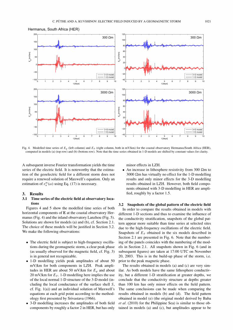
Fig. 4. Modelled time series of Eϕ (left column) and Eϑ (right column, both in mV/km) for the coastal observatory Hermanus/South Africa (HER),computed in models (a) (top row) and (b) (bottom row). Note that the time series obtained in 1-D models are shifted by constant values for clarity.

A subsequent inverse Fourier transformation yields the timeseries of the electric field. It is noteworthy that the estima-tion of the geoelectric field for a different storm does notrequire a renewed solution of Maxwell’s equation. Only anestimation of εm

n (ω) using Eq. (17) is necessary.

3. Results3.1 Time series of the electric field at observatory loca-

tionsFigures 4 and 5 show the modelled time series of both

horizontal components of E at the coastal observatory Her-manus (Fig. 4) and the inland observatory Lanzhou (Fig. 5).Solutions are shown for models (a) and (b), cf. Section 2.1.The choice of these models will be justified in Section 3.2.We make the following observations:

• The electric field is subject to high-frequency oscilla-tions during the geomagnetic storm, a clear peak phase(as usually observed for the magnetic field, cf. Fig. 3)is in general not recognizable.

• 1-D modelling yields peak amplitudes of about 50mV/km for both components in LZH. Peak ampli-tudes in HER are about 50 mV/km for Eϕ and about20 mV/km for Eϑ . 1-D modelling here implies the useof the local normal 1-D structure of the 3-D model (in-cluding the local conductance of the surface shell S,cf. Fig. 1(a)) and an individual solution of Maxwell’sequations at each grid point according to the method-ology first presented by Srivastava (1966).

• 3-D modelling increases the amplitudes of both fieldcomponents by roughly a factor 2 in HER, but has only

minor effects in LZH.• An increase in lithosphere resistivity from 300 �m to

3000 �m has virtually no effect for the 1-D modellingresults and only minor effects for the 3-D modellingresults obtained in LZH. However, both field compo-nents obtained with 3-D modelling in HER are ampli-fied, roughly by a factor 1.5.

3.2 Snapshots of the global pattern of the electric fieldIn order to compare the results obtained in models with

different 1-D sections and thus to examine the influence ofthe conductivity stratification, snapshots of the global pat-tern appear more suitable than time series at selected sitesdue to the high-frequency oscillations of the electric field.Snapshots of Eϑ obtained in the six models described inSection 2.1 are presented in Fig. 6. Note that the number-ing of the panels coincides with the numbering of the mod-els in Section 2.1. All snapshots shown in Fig. 6 (and insubsequent figures) are taken at 17:00 UTC on November20, 2003. This is in the build-up phase of the storm, i.e.prior to the peak magnetic phase.

The results obtained in models (a) and (c) are very sim-ilar. As both models have the same lithosphere conductiv-ity, but a different 1-D stratification at greater depths, weconclude that the conductivity structure at depths greaterthan 100 km has only minor effects on the field pattern.The same conclusions can be made when comparing theresults obtained in models (b) and (d). The field patternobtained in model (e) (the original model derived by Babaet al. (2010) for the Philippine Sea) is similar to those ob-tained in models (a) and (c), but amplitudes appear to be


Fig. 5. Modelled time series of Eϕ (left column) and Eϑ (right column, both in mV/km) for the inland observatory Lanzhou/China (LZH), computedin models (a) (top row) and (b) (bottom row). Note that the time series obtained in 1-D models are shifted by constant values for clarity.

Fig. 6. Snapshots of the latitudinal component of the estimated electric field, Eϑ (in mV/km), at 17:00 UTC on November 20, 2003 in six differentconductivity models (a)–(f) (described in Section 2.1).

slightly lower. Similarly, the pattern obtained in model (f)(the original model derived by Baba et al. (2010) for theNorth Pacific) is slightly less pronounced than the patternsobtained in models (b) and (d), and amplitudes are slightlylower. We attribute this difference to the increase in con-ductivity at shallow depths in the models derived by Babaet al. (2010) (cf. Fig. 1(b)).

A cross-comparison of both rows in Fig. 6 indicates thatstronger and more pronounced fields are obtained in modelswith larger transversal resistance of the lithosphere. As thedifferences between the rows are significantly larger thanthose within each row, we conclude that our basic models(a) and (b) are good representatives and will thus in thefollowing concentrate on the results obtained in models (a)and (b). Note that a comparison of Eϕ in the various models

leads to the same conclusions, as well as the examination ofsnapshots at different instants.

We are especially interested in investigating the effectsarising from the laterally non-uniform surface layer S. Tothis purpose, we present results in form of the “anomalous”electric field, which is computed as difference between our3-D modelling results and results obtained in a “local 1-D” model. Local 1-D modelling here implies the use ofthe local normal 1-D structure of the 3-D model (includingthe local conductance of the surface shell S) and a solutionof Maxwell’s equations separately performed at each gridpoint. Expressions for the (frequency domain) electric fieldemerging due to induction by a source of our type in 1-Dconductivity models are presented in Appendix H of Ku-vshinov and Semenov (2012).


Fig. 7. Snapshots of the modelled anomalous electric field (left column: Eϕ , right column: Eϑ , both in mV/km) at 17:00 UTC on November 20, 2003,computed in models (a) (top row) and (b) (bottom row). The black bars through North America and Australia denote the profiles shown in Fig. 8.

Fig. 8. Profiles of the modelled anomalous electric field (left column: Eϕ , right column: Eϑ , both in mV/km) through North America and Australia(see also Fig. 7) at 17:00 UTC on November 20, 2003. The black dashed lines mark the coast.

Snapshots of the anomalous Eϑ and Eϕ for the sameinstant as in Fig. 6, computed in models (a) and (b), arepresented in Fig. 7. The black latitude-parallel lines throughNorth America and Australia indicate the profiles of electricfield versus longitude that are drawn in Fig. 8. We make thefollowing observations:

• As expected, the anomalous field is very small in-side continents and oceans, but pronounced in regionswhere conductance varies laterally on short scales, es-pecially at the coasts.

• Largest amplitudes are observed at long east and west

coasts, e.g. the Americas or southern Africa. This re-flects the geometry of the source (the magnetosphericring current).

• An increase of lithosphere resistivity from 300 �m to3000 �m leads to an amplification of the componentsof the anomalous electric field by roughly a factor 2 atcoastal sites.

• The penetration width of the anomalous field is alsogoverned by lithosphere resistivity. Dependent on thesite, massive enhancements are observed up to 400 kminland in the case of a 300 �m lithosphere and upto 600 km inland in the more resistive case (Fig. 8;


note that 1◦ of longitude corresponds to 100 km in theprofile through Australia and to 85 km in the profilethrough North America).

• In latitude-parallel profiles through continents, theanomalous Eϕ exhibits an axial symmetry, while theanomalous Eϑ is anti-symmetric. This observationconfirms previous results by Kuvshinov et al. (1999)obtained in simplified conceptual models. Note thatthere is no enhancement of Eϑ at the Australian westcoast for the chosen moment, cf. Fig. 8.

Our results stress the need of 3-D modelling in an envi-ronment with large lateral variations in conductivity. Theamplifications observed at coasts are at least on the samelevel as the maximum amplitudes obtained in 1-D models.As previously shown in Fig. 4, using a 1-D model might re-sults in an underestimation of the peak amplitudes of thegeoelectric field during a geomagnetic storm by a factor2–3 at coastal sites. Due to the high temporal variabilityof the geoelectric field, coastal enhancements vary signifi-cantly during a geomagnetic storm.

4. Discussion and Conclusions4.1 Summary

We have presented a numerical scheme for a time do-main estimation of the global electric field induced by ageomagnetic storm with realistic spatio-temporal structure,derived from measurements of the horizontal component ofthe magnetic field at worldwide distributed observatories.A conductivity model of Earth’s interior with a realistic lat-erally heterogeneous surface layer representing oceans andcontinents was used.

The results could be obtained within a few hours, if theobservatory data were available and pre-processed (edited,checked for consistency etc.). It is noteworthy that this es-timate does not depend on the complexity and resolution ofthe 3-D conductivity model, since the responses for induc-tion in a given 3-D model by elementary sources (in caseof a geomagnetic storm described by spherical harmonics)can be calculated beforehand and archived. To obtain thegeoelectric field for a specific storm, it is just necessary toreconstruct the spatio-temporal form of the external sourceresponsible for this storm and to convolve the source fieldwith the precomputed 3-D responses. We believe that ournumerical scheme would be a useful tool to estimate quanti-tatively the space weather hazard associated with excessiveGIC arising in ground-based conductor networks (such aspower lines) during major geomagnetic storms.4.2 Effect of oceans and lithosphere

Model studies based on our numerical scheme revealedsubstantial differences between the electric fields generatedin 3-D and 1-D models, even if the 1-D model makes useof the local vertical conductivity structure. As expected, thedifferences are mainly marked at the coasts. The anomalouselectric field, computed as difference between the electricfields obtained in 3-D and 1-D models, can penetrate up tomore than 500 km inland (depending on the site and thelocal conductivity structure). Anomalous amplitudes are atleast as large as the amplitudes calculated in a 1-D model.Peak amplitudes of a geomagnetic storm at coastal sites are

hence underestimated by a factor 2–3 when using a 1-Dmodel. The 3-D modelling results state that coastal areasare in danger of experiencing electric field amplitudes ofup to 200 mV/km during a typical magnetic storm. Longeast and west coasts like the Americas, southern Africa orAustralia and narrow land bridges like Panama seem to beespecially endangered.

The resistivity of the lithosphere is a critical parameterwhen estimating amplitudes of the electric field. Resistivi-ties of 300 �m and 3000 �m, representing realistic bound-ary values for Earth’s lithosphere, were tested in this study.Lithosphere resistivity mainly affects the electric field atcoastal sites. The amplitudes of the anomalous electricfield were doubled in the model with a lithosphere of 3000�m, and the “coastal region”, in which the anomalous fieldshows enhanced amplitudes, was significantly wider. Theinfluences of the conductivity distribution at greater depthsand the precise stratification within the lithosphere on theresults were minor in comparison with the integrated litho-sphere resistivity.

According to our modelling results, a precise estimate ofthe lithosphere resistivity in the region of interest is cru-cial in order to obtain a trustworthy estimate of the actualelectric field. In this study, we considered a model witha lithosphere of laterally uniform thickness and resistivity.While the chosen lithosphere thickness of 100 km agreeswith the global average, it is well-known that lithospherethickness is very variable on Earth and ranges from few kmat mid-ocean ridges to several 100 km below old continen-tal shields. The choice of a laterally uniform lithosphereis thus a limitation of our work; it was however necessary,since thickness and resistivity of the lithosphere are poorlyresolved on a global scale. We want to stress in this con-text that the numerical solution discussed in this paper isfully 3-D and thus can readily adopt models with a laterallyvariable lithosphere once reliable information about suchvariability is available.4.3 Estimates of the electric field at polar latitudes

In this paper, we discussed the geoelectric field inducedby a large-scale magnetospheric source that dominates inmid-latitudes. However, it is well known that one can ex-pect larger signals in polar regions due to substorm geo-magnetic disturbances (Pirjola and Viljanen, 1994). The re-covery of the spatio-temporal structure of the auroral iono-spheric source, which is responsible for this activity, is morechallenging due to the large variability of the auroral sourceboth in time and space.

One of the ways to determine realistic auroral currentson a semi-global scale (in the whole polar cap) consists ofcollecting the data from high-latitude geomagnetic obser-vatories and polar magnetometer arrays (e.g. IMAGE andMIRACLE arrays in Scandinavia, DTU and MAGIC arraysin Greenland, CARISMA array in Canada etc.) and thenreconstructing the auroral current, for example by exploit-ing an approach based on elementary current systems (e.g.Amm, 2001; Sun and Egbert, 2012). Note that this ap-proach was used by Pulkkinen and Engels (2005), who anal-ysed the influence of 3-D induction effects on ionosphericcurrents during geomagnetic substorms.

Once the auroral source is quantified, a similar numeri-


cal scheme as described above, however with two modifi-cations, can be implemented in order to calculate the geo-electric field caused by a geomagnetic substorm. One mod-ification concerns the description of the substorm source—instead of using a spherical harmonics representation, onecan mimic the auroral ionospheric current by elementarycurrent systems. Another modification applies to the 3-Dconductivity model. Since substorm magnetic variations arecharacterized by periods between a few tens of seconds andtens of minutes, one cannot exploit a model in which thesurface layer is approximated by a thin shell, as it was donein this paper. The variable thickness of this layer is im-portant in this period range, thus a full 3-D model (includ-ing bathymetry) should be considered. However, as men-tioned in Section 4.1, the complexity and resolution of the3-D conductivity model has no effect on the computationalcost of the source modelling for a specific substorm. As inthe case of a large-scale geomagnetic storm, a model of theelectric field due to a specific substorm for the whole po-lar cap could be obtained within a few hours when using astandard workstation for computations. Note again that thisestimate does not account for the efforts of collecting andpre-processing the data and for the 3-D calculations of themagnetic field due to elementary sources.

Semi-global estimates of the geoelectric field induced bya realistic geomagnetic substorm in a realistic 3-D conduc-tivity model accounting for bathymetry and non-uniformlithosphere will be the subject of a subsequent publication.

Acknowledgments. The authors express their gratitude to thestaff of the geomagnetic observatories who have collected and dis-tributed the data. We thank Dr. Alan Thomson for discussion onthe manuscript and Dr. Ikuko Fujii and an anonymous reviewerfor helpful comments. This work has been supported by the SwissNational Science Foundation under grant No. 2000021-140711/1.

ReferencesAmm, O., The elementary current method for calculating ionospheric cur-

rent systems from multisatellite and ground magnetometer data, J. Geo-phys. Res., 106, 24843–24855, 2001.

Aster, R. C., B. Borchers, and C. H. Thurber, Parameter Estimation andInverse Problems, Elsevier Academic Press, 2005.

Baba, K., H. Utada, T. Goto, T. Kasaya, H. Shimizu, and N. Tada, Electricalconductivity imaging of the Philippine Sea upper mantle using seafloormagnetotelluric data, Phys. Earth. Planet. Inter., 183, 44–62, 2010.

Beamish, D., T. D. G. Clark, E. Clarke, and A. W. P. Thomson, Geomagnet-ically induced currents in the UK: Geomagnetic variations and surfaceelectric fields, J. Atmos. Sol. Terr. Phys., 64, 1779–1792, 2002.

Cox, C. J., Electromagnetic induction in the oceans and inferences on theconstitution of the earth, Geophys. Surv., 7, 137–156, 1980.

Everett, M. E., S. Constable, and C. G. Constable, Effects of near-surfaceconductance on global satellite induction responses, Geophys. J. Int.,153, 277–286, 2003.

Fainberg, E. B., Electromagnetic induction in the world ocean, Geophys.Surv., 4, 157–171, 1980.

Gilbert, J., Modeling the effect of the ocean-land interface on in-duced electric fields during geomagnetic storms, Space Weather, 3,doi:10.1029/2004SW000120, 2005.

Kappenman, J., L. Zanetti, and W. Radasky, Geomagnetic storms canthreaten electric power grid, Earth in Space, 9, 9–11, 1997.

Kuvshinov, A., 3-D Global induction in the oceans and solid Earth: recentprogress in modeling magnetic and electric fields from sources of mag-netospheric, ionospheric and oceanic origin, Surv. Geophys., 29, 139–186, 2008.

Kuvshinov, A. and N. Olsen, A global model of mantle conductivity de-rived from 5 years of CHAMP, Ørsted, and SAC-C magnetic data, Geo-phys. Res. Lett., 33, doi:10.1029/2006GL027083, 2006.

Kuvshinov, A. and A. Semenov, Global 3-D imaging of mantle electri-cal conductivity based on inversion of observatory C-responses I. Anapproach and its verification, Geophys. J. Int., 189, doi:10.1111/j.1365–246X.2011.05349.x, 2012.

Kuvshinov, A. V., D. B. Avdeev, and O. V. Pankratov, Global induction bySq and Dst sources in the presence of oceans: bimodal solutions for non-uniform spherical surface shells above radially symmetric Earth modelsin comparison to observations, Geophys. J. Int., 137, 630–650, 1999.

Laske, G. and G. Masters, A global digital map of sediment thickness, EosTrans. AGU, 78, F483, 1997.

Love, J. J., Magnetic monitoring of Earth and space, Physics Today, 61,31–37, 2008.

Manoj, C., A. Kuvshinov, S. Maus, and H. Luehr, Ocean circulation gen-erated magnetic signals, Earth Planets Space, 58, 429–437, 2006.

Olsen, N. and A. Kuvshinov, Modeling the ocean effect of geomagneticstorms, Earth Planets Space, 56, 525–530, 2004.

Parkinson, W. D. and F. W. Jones, The geomagnetic coast effect, Rev.Geophys., 17, 1999–2015, 1979.

Pirjola, R., Geomagnetically induced currents during magnetic storms,IEEE Trans Plasma Sci, 28, 1867–1873, 2000.

Pirjola, R. and A. Viljanen, Geomagnetically induced currents in theFinnish high-voltage power system, a geophysical review, Surv. Geo-phys., 15, 383–408, 1994.

Pulkkinen, A. and M. Engels, The role of 3-D geomagnetic induction in thedetermination of the ionospheric currents from the ground geomagneticdata, Ann. Geophys., 23, 909–917, 2005.

Pulkkinen, A., M. Hesse, M. Kuznetsova, and L. Rastatter, First principlesmodeling of geomagnetically induced electromagnetic fields and cur-rents from upstream solar wind to the surface of the Earth, Ann. Geo-phys., 25, 881–893, 2007.

Rikitake, T. and Y. Honkura, Developments in Earth and planetary sci-ences, in Solid Earth Geomagnetism, vol. 5, edited by Rikitake, T., TerraScientific Publishing Company, 1985.

Srivastava, S. P., Theory of the magnetotelluric method for a sphericalconductor, Geophys. J. R. Astron. Soc., 11, 373–387, 1966.

Sun, J. and G. Egbert, Spherical decomposition of electromagnetic fieldsgenerated by quasi-static currents, Int. J. Geomath., 3, 279–295, 2012.

Thomson, A. W. P., A. J. McKay, E. Clarke, and S. J. Reay, Surface electricfields and geomagnetically induced currents in the Scottish Power gridduring the 30 October 2003 geomagnetic storm, Space Weather, 3,doi:10.1029/2005SW000156, 2005.

Thomson, A. W. P., A. J. McKay, and A. Viljanen, A review of progressin modelling of induced geoelectric and geomagnetic fields with specialregard to induced currents, Acta Geophys., 57, 209–219, 2009.

C. Puthe (e-mail: [email protected]) and A. Kuvshinov

towards quantitative assessment of the hazard from · pdf filetowards quantitative assessment...

Documents