Towards in-situ visualization integrated Earth System Models:

RegESM 1.1 regional modeling system

Ufuk Utku Turuncoglu 1

1Informatics Institute, Istanbul Technical University, 34469, Istanbul, Turkey

Correspondence: Ufuk Utku Turuncoglu (ufuk.turuncoglu@itu.edu.tr)

Abstract. The data volume produced by regional and global multi-component Earth System Models are rapidly increasing

because of the improved spatial and temporal resolution of the model components, the sophistication of the used numerical

models regarding represented physical processes and their complex non-linear interactions. In particular, very small time step

needs to be defined in non-hydrostatic high-resolution modeling applications to represent the evolution of the fast-moving pro-

cesses such as turbulence, extra-tropical cyclones, convective lines, jet streams, internal waves, vertical turbulent mixing and5

surface gravity waves. Consequently, the employed small time steps cause extra computation and disk input-output overhead

in the modeling system even if today’s most powerful high-performance computing and data storage systems are considered.

Analysis of the high volume of data from multiple Earth System Model components at different temporal and spatial resolution

also poses a challenging problem to efficiently perform integrated data analysis of the massive amounts of data by relying on

the conventional post-processing methods available today. This study mainly aims to explore the feasibility and added value of10

integrating existing in-situ visualization and data analysis methods with the model coupling framework to increase interoper-

ability between multi-component simulation code and data processing systems by providing easy to use, efficient, generic and

standardized modeling environment for Earth system science applications. The new data analysis approach enables simultane-

ous analysis of the vast amount of data produced by multi-component regional Earth System Models during the runtime. The

presented methodology also aims to create an integrated modeling environment for analyzing fast-moving processes and their15

evolution in both time and space to support a better understanding of the underplaying physical mechanisms. The state-of-art

approach can also be employed to solve common problems in the model development cycle: designing new sub-grid scale

parametrizations that requires inspecting the integrated model behavior in a higher temporal and spatial scale simultaneously

and supporting visual debugging of the multi-component modeling systems, which usually are not facilitated by existing model

coupling libraries and modeling systems.20

1 Introduction

The multi-scale and inherently coupled Earth System Models (ESMs) make them challenging to study and understand. Rapid

developments in Earth system science, as well as in high-performance computing and data storage systems, have enabled fully

coupled regional or global ESMs to better represent relevant processes, complex climate feedbacks, and interactions among

the coupled components. In this context, regional ESMs are employed when the spatial and temporal resolution of the global25

1

climate models are not sufficient to resolve local features such as complex topography, land-sea gradients and the influence

of human activities in a smaller spatial scale. Along with the development of the modeling systems, specialized software

libraries for the model coupling become more and more critical to reduce the complexity of the coupled model development

and increase the interoperability, reusability, and efficiency of the existing modeling systems. Currently, the existing model

coupling software libraries have two main categories: couplers and coupling frameworks.5

Couplers are mainly specialized in performing specific operations more efficiently and quickly such as coordination of

components and interpolation among model components. For example, OASIS3 (Valcke, 2013) uses multiple executable ap-

proaches for coupling model components but sequentially performing internal algorithms such as sparse matrix multiplication

(SMM) operation for interpolation among model grids become a bottleneck along with increased spatial resolution of the model

components. To overcome the problem, OASIS4 uses parallelism in its internal algorithms (Redler et al., 2010), but OASIS310

coupler interfaced with the Model Coupling Toolkit (MCT; Jacob et al., 2005; Larson et al., 2005) to develop OASIS3-MCT

that provides a parallel implementation of interpolation and data exchange. Besides generic couplers like OASIS, domain-

specific couplers such as Oceanographic Multi-purpose Software Environment (OMUSE; Pelupessy et al., 2017) that aims to

provide a homogeneous environment for ocean modeling to make verification of simulation models with different codes and nu-

merical methods and Community Surface Dynamics Modeling System (CSDMS; Overeem et al., 2013) to develop integrated15

software modules for modeling of Earth surface processes are introduced.

A coupling framework is as an environment for coupling model components through a standardized calling interface and

aims to reduce the complexity of regular tasks such as performing spatial interpolation across different computational grids

and transferring data among model components to increase the efficiency and interoperability of multi-component modeling

systems. Besides, the synchronization of the execution of individual model components, a coupling framework can simplify20

the exchange of metadata related to model components and exchanged fields through the use of existing conventions such as

CF (Climate and Forecast) convention. The Earth System Modeling Framework (ESMF) is one of the most famous examples

of this approach (Theurich et al., 2016). The ESMF consists of a standardized superstructure for coupling components of Earth

system applications through a robust infrastructure of high-performance utilities and data structures that ensure consistent

component behavior (Hill et al., 2004). The ESMF framework is also extended to include the National Unified Operational25

Prediction Capability (NUOPC) layer. The NUOPC layer simplifies component synchronization and run sequence by providing

additional programming interface between coupled model and ESMF framework through the use of NUOPC “cap”. In this case,

a NUOPC “cap” is a Fortran module that serves as the interface to a model when it is used in a NUOPC-based coupled system.

The term “cap” is used because it is a small software layer that sits on top of a model code, making calls into it and exposing

model data structures in a standard way. In addition to generic modeling framework like ESMF, Modular System for Shelves30

and Coasts (MOSSCO; Lemmen et al., 2018) creates a state-of-art domain and process coupling system by taking advantage of

both ESMF and Framework for Aquatic Biogeochemical Models (FABM; Bruggeman and Bolding, 2014) for marine coastal

Earth system community.

The recent study of Alexander and Easterbrook (2015) to investigate the degree of modularity and design of the existing

global climate models reveals that the majority of the models use central couplers to support data exchange, spatial inter-35

2

polation, and synchronization among model components. In this approach, direct interaction does not have to occur between

individual model components or modules, since the specific coupler component manages the data transfer. This approach is also

known as the hub-and-spoke method of building a multi-component coupled model. A key benefit of using a hub-and-spoke

approach is that it creates a more flexible and efficient environment for designing sophisticated multi-component modeling sys-

tem regarding represented physical processes and their interactions. The development of the more complex and high-resolution5

modeling systems leads to an increased demand for both computational and data storage resources. In general, the high volume

of data produced by the numerical modeling systems may not allow storing all the critical and valuable information to use later,

despite recent advances in storage systems. As a result, the simulation results are stored in a limited temporal resolution (i.e.,

monthly averages), which are processed after numerical simulations finished (post-processing). The poor representation of the

results of numerical model simulations prevents to analyze the fast-moving processes such as extreme precipitation events,10

convection, turbulence and non-linear interactions among the model components in a high temporal and spatial scale with the

conventional post-processing approach.

The analysis of leading high-performance computing systems reveals that the rate of disk input-output (I/O) performance

is not growing at the same speed as the peak computational power of the systems (Ahern, 2012; Ahrens, 2015). The recent

report of U.S. Department of Energy (DOE) also indicates that the expected rate of increase in I/O bandwidth (100 times)15

will be slower than the peak system performance (500 times) of the new generations of exascale computers (Ashby et al.,

2010). Besides, the movement of large volumes of data across relatively slow network bandwidth servers fails to match the

ultimate demands of data processing and to archive tasks of the present high-resolution multi-component ESMs. As a result,

the conventional post-processing approach has become a bottleneck in monitoring and analysis of fast-moving processes that

require very high spatial resolution, due to the present technological limitations in high-performance computing and storage20

systems (Ahrens et al., 2014). In the upcoming computing era, state-of-art new data analysis and visualization methods are

needed to overcome the above limitations evocatively.

Besides the conventional data analysis approach, the so-called in-situ visualization and co-processing approaches allow re-

searchers to analyze the output while running the numerical simulations simultaneously. The coupling of computation and

data analysis helps to facilitate efficient and optimized data analysis and visualization pipelines and boosts the data analysis25

workflow. Recently, a number of in-situ visualization systems for analyzing numerical simulations of Earth system processes

have been implemented. For instance, the ocean component of Model for Prediction Across Scales (MPAS) has been integrated

with an image-based in-situ visualization tool to examine the critical elements of the simulations and reduce the data needed

to preserve those elements by creating a flexible work environment for data analysis and visualization (Ahrens et al., 2014;

O’Leary et al., 2016). Additionally, the same modeling system (MPAS-Ocean) has been used to study eddies in large-scale,30

high-resolution simulations. In this case, the in-situ visualization workflow is designed to perform eddy analysis at higher spa-

tial and temporal resolutions than available with conventional post-processing facing storage size and I/O bandwidth constraints

(Woodring et al., 2016). Moreover, a regional weather forecast model (Weather Research and Forecasting Model; WRF) has

been integrated with in-situ visualization tool to track cyclones based on an adaptive algorithm (Malakar et al., 2012). Despite

the lack of generic and standardized implementation for integrating model components with in-situ visualization tools, the35

3

previous studies have shown that in-situ visualization can produce analyses of simulation results, revealing many details in an

efficient and optimized way. It is evident that more generic implementations could facilitate smooth integration of the existing

standalone and coupled ESMs with available in-situ visualization tools (Ahrens et al., 2005; Ayachit, 2015; Childs et al., 2012)

and improve interoperability between such tools and non-standardized numerical simulation codes.

The main aim of this paper is to explore the added value of integrating in-situ analysis and visualization methods with a5

model coupling framework (ESMF) to provide in-situ visualization for easy to use, generic, standardized and robust scientific

applications of Earth system modeling. The implementation allows existing ESMs coupled with the ESMF library to take

advantage of in-situ visualization capabilities without extensive code restructuring and development. Moreover, the integrated

model coupling environment allows sophisticated analysis and visualization pipelines by combining information coming from

multiple ESM components (i.e., atmosphere, ocean, wave, land-surface) in various spatial and temporal resolutions. Detailed10

studies of fundamental physical processes and interactions among model components are vital to the understanding of complex

physical processes and could potentially open up new possibilities for the development of ESMs.

2 The Design of the Modeling System

The RegESM (Regional Earth System Model; 1.1) modeling system can use five different model components to support many

different modeling applications that might require detailed representation of the interactions among different Earth system15

processes (Fig. 1a-b). The implementation of the modeling system follows the hub-and-spoke architecture. The driver that is

responsible for the orchestration of the overall modeling system resides in the middle and acts as a translator among model

components (atmosphere, ocean, wave, river routing, and co-processing). In this case, each model component introduces its

NUOPC cap to plug into the modeling system. The modeling system is validated in different model domains such as Caspian

Sea (Turuncoglu et al., 2013), Mediterranean Basin (Surenkok and Turuncoglu, 2015; Turuncoglu and Sannino, 2017), and20

Black Sea Basin.

2.1 Atmosphere Models (ATM)

The flexible design of RegESM modeling system allows choosing a different atmospheric model component (ATM) in the

configuration of the coupled model for a various type of application. Currently, two different atmospheric model is compatible

with RegESM modeling system: (1) RegCM4 (Giorgi et al., 2012), which is developed by the Abdus Salam International25

Centre for Theoretical Physics (ICTP) and (2) the Advanced Research Weather Research and Forecasting (WRF) Model (ARW;

Skamarock et al., 2005), which is developed and sourced from National Center for Atmospheric Research (NCAR). In this

study, RegCM 4.6 is selected as an atmospheric model component because the current implementation of WRF coupling

interface is still experimental and does not support coupling with co-processing component yet, but the next version of the

modeling system (RegESM 1.2) will be able to couple WRF atmospheric model with co-processing component. The NUOPC30

cap of atmospheric model components defines state variables (i.e., sea surface temperature, surface wind components), rotates

4

the winds relative to Earth, apply unit conversions and perform vertical interpolation to interact with the newly introduced

co-processing component.

2.1.1 RegCM

The dynamical core of the RegCM4 is based on the primitive equation, hydrostatic version of the National Centre for At-

mospheric Research (NCAR) and Pennsylvania State University mesoscale model MM5 (Grell, 1995). The latest version5

of the model (RegCM 4.6) also supports non-hydrostatic dynamical core to support applications with high spatial resolu-

tions (< 10 km). The model includes two different land surface models: (1) Biosphere-Atmosphere Transfer Scheme (BATS;

Dickinson et. al., 1989) and (2) Community Land Model (CLM), version 4.5 (Tawfik and Steiner, 2011). The model also in-

cludes specific physical parameterizations to define air-sea interaction over the sea and lake (one-dimensional lake model;

Hostetler et al., 1993). The Zeng Ocean Air-Sea Parameterization (Zeng et al., 1998) is extended to introduce the atmosphere10

model as a component of the coupled modeling system. In this way, the atmospheric model can exchange both two and three-

dimensional fields with other model components such as an ocean, wave and river routing components that are active in an

area inside of the atmospheric model domain as well as in-situ visualization component.

2.1.2 WRF

The WRF model consists of fully compressible non-hydrostatic equations, and the prognostic variables include the three-15

dimensional wind, perturbation quantities of pressure, potential temperature, geo-potential, surface pressure, turbulent kinetic

energy and scalars (i.e., water vapor mixing ratio, cloud water). The model is suitable for a broad range of applications and

has a variety of options to choose parameterization schemes for the planetary boundary layer (PBL), convection, explicit

moisture, radiation, and soil processes to support analysis of different Earth system processes. The PBL scheme of the model

has a significant impact on exchanging moisture, momentum, and energy between air and sea (and land) due to the used20

alternative surface layer options (i.e., drag coefficients) in the model configuration. A few modifications are done in WRF

(version 3.8.1) model itself to couple it with RegESM modeling system. These modifications include rearranging of WRF

time-related subroutines, which are inherited from the older version of ESMF Time Manager API (Application Programming

Interface) that was available in 2009, to compile model with the newer version of ESMF library (version 7.1.0) together with

the older version that requires mapping of time manager data types between old and new versions.25

2.2 Ocean Models (OCN)

The current version of the coupled modeling system supports two different ocean model components (OCN): (1) Regional

Ocean Modeling System (ROMS revision 809; Shchepetkin and McWilliams, 2005; Haidvogel et al., 2008), which is devel-

oped and distributed by Rutgers University and (2) MIT General Circulation Model (MITgcm version c63s; Marshall et al.,

1997a, b). In this case, ROMS and MITgcm models are selected due to their large user communities and different vertical30

grid representations. Although the selection of ocean model components depends on user experience and application, often

5

the choice of vertical grid system has a determining role in some specific applications. For example, the ROMS ocean model

uses terrain following (namely s-coordinates) vertical grid system that allows better representation of the coastal processes but

MITgcm uses z levels and generally used for the applications that involve open oceans and seas. Similar to the atmospheric

model component, both ocean models are slightly modified to allow data exchange with the other model components. In the

current version of the coupled modeling system, there is no interaction between wave and ocean model components, which

could be crucial for some applications (i.e., surface ocean circulation and wave interaction) that need to consider the two-way

interaction between waves and ocean currents. The exchange fields defined in the coupled modeling system between ocean5

and atmosphere strictly depend on the application and the studied problem. In some studies, the ocean model requires heat,

freshwater and momentum fluxes to be provided by the atmospheric component, while in others, the ocean component re-

trieves surface atmospheric conditions (i.e., surface temperature, humidity, surface pressure, wind components, precipitation)

to calculate fluxes internally, by using bulk formulas (Turuncoglu et al., 2013). In the current design of the coupled modeling

system, the driver allows selecting the desired exchange fields from the predefined list of the available fields. The exchange10

field list is a simple database with all known fields that can be exported or imported by the component. In this way, the coupled

modeling system can be adapted to different applications without any code customizations in both the driver and individual

model components.

2.2.1 ROMS

The ROMS is a three-dimensional, free-surface, terrain-following numerical ocean model that solves the Reynolds-averaged15

Navier-Stokes equations using the hydrostatic and Boussinesq assumptions. The governing equations are in flux form, and

the model uses Cartesian horizontal coordinates and sigma vertical coordinates with three different stretching functions. The

model also supports second, third and fourth order horizontal and vertical advection schemes for momentum and tracers via its

preprocessor flags.

2.2.2 MITgcm20

The MIT general circulation model (MITgcm) is a generic and widely used ocean model that solves the Boussinesq form

of Navier-Stokes equations for an incompressible fluid. It supports both hydrostatic and non-hydrostatic applications with a

spatial finite-volume discretization on a curvilinear computational grid. The model has an implicit free surface in the surface and

partial step topography formulation to define vertical depth layers. The MITgcm model supports different advection schemes

for momentum and tracers such as centered second order, third-order upwind and second-order flux limiters to support a variety25

of applications. The model used in the coupled modeling system is slightly modified by ENEA to allow data exchange with

other model components. The detailed information about the regional applications of the MITgcm ocean model was initially

described in the study of Artale et al. (2010) using PROTHEUS modeling system specifically developed for the Mediterranean

Sea.

6

2.3 Wave Model (WAV)30

Surface waves play a crucial role in the dynamics of PBL in the atmosphere and the currents in the ocean. Therefore, the

wave component is included in the coupled modeling system to have a better representation of atmospheric PBL and surface

conditions (i.e., surface roughness, friction velocity, wind speed). In this case, the wave component is based on WAM Cycle-4

(4.5.3-MPI). The WAM is a third-generation model without any assumption on the spectral shape (Monbaliu et al., 2000). It

considers all the main processes that control the evolution of a wave field in deep water, namely the generation by wind, the

nonlinear wave–wave interactions, and also white-capping. The model is initially developed by Helmholtz-Zentrum Geesthacht5

(GKSS, now HZG) in Germany. The original version of the WAM model is slightly modified to retrieve surface atmospheric

conditions (i.e., wind speed components or friction velocity and wind direction) from the RegCM4 atmospheric model and

send back calculated surface roughness. In the current version of the modeling system, wave component cannot be coupled

with the WRF model due to the missing modifications in the WRF side. In the RegCM4, the received surface roughness is used

to calculate air-sea transfer coefficients and fluxes over sea using Zeng ocean air-sea parameterization (Zeng et al., 1998). In10

this design, it is also possible to define a threshold for maximum roughness length (the default value is 0.02 m) and friction

velocity (the default value is 0.02 m) in the configuration file of RegCM4 to ensure the stability of the overall modeling

system. The initial results to investigate the added value of atmosphere-wave coupling in the Mediterranean Sea can be found

in Surenkok and Turuncoglu (2015).

2.4 River Routing Model (RTM)15

To simulate the lateral freshwater fluxes (river discharges) at the land surface and to provide river discharge to ocean model

component, the RegESM modeling system uses Hydrological Discharge (HD, version 1.0.2) model developed by Max Planck

Institute (Hagemann and Dumenil, 1998; Hagemann and Lydia, 2001). The model is designed to run in a fixed global regular

grid with 0.5◦ horizontal resolution using daily time series of surface runoff and drainage as input fields. In this case, the model

uses the pre-computed river channel network to simulate the horizontal transport of the runoff within model watersheds using20

different flow processes such as overland flow, baseflow and riverflow. The river routing model (RTM) plays an essential role

in the freshwater budget of the ocean model by closing the water cycle between the atmosphere and ocean model components.

The original version of the model is slightly modified to support interaction with the coupled model components. To close

water cycle between land and ocean, model retrieves surface and sub-surface runoff from the atmospheric component (RegCM

or WRF) and provides estimated river discharge to the selected ocean model component (ROMS or MITgcm). In the current25

design of the driver, rivers can be represented in two different ways: (1) individual point sources that are vertically distributed

to model layers, and (2) imposed as freshwater surface boundary condition like precipitation (P) or evaporation minus pre-

cipitation (E-P). In this case, the driver configuration file is used to select the river representation type (1 or 2) for each river

individually. The first option is preferred if river plumes need to be defined correctly by distributing river discharge vertically

among the ocean model vertical layers. The second option is used to distribute river discharge to the ocean surface when there30

is a need to apply river discharge to a large areal extent close to the river mouth. In this case, a special algorithm implemented

7

in NUOPC cap of ocean model components (ROMS and MITgcm) is used to find affected ocean model grids based on the

effective radius (in km) defined in the configuration file of the driver.

2.5 The Driver: RegESM

The RegESM (version 1.1) is completely redesigned and improved version of the previously used and validated coupled

atmosphere-ocean model (RegCM-ROMS) to study the regional climate of Caspian Sea and its catchment area (Turuncoglu et al.,

2013). To simplify the design and to create more generic, extensible and flexible modeling system that aims to support easy

integration of multiple model components and applications, the RegESM uses a driver to implement the hub-and-spoke ap-5

proach. In this case, all the model components are combined using ESMF (version 7.1.0) framework to structure coupled

modeling system. The ESMF framework is selected because of its unique online re-gridding capability, which allows the driver

to perform different interpolation types (i.e., bilinear, conservative) over the exchange fields (i.e., sea surface temperature, heat

and momentum fluxes) and the NUOPC layer. The NUOPC layer is a software layer built on top of the ESMF. It refines the

capabilities of ESMF by providing a more precise definition of what it means for a model to be a component and how compo-10

nents should interact and share data in a coupled system. The ESMF also provides the capability of transferring computational

grids in memory among the model components, which has critical importance in the integration of the modeling system with

a co-processing environment (see also Sect. 3). The RegESM modeling system also uses ESMF and NUOPC layer to support

various configuration of component interactions such as defining multiple coupling time steps among the model components.

An example configuration of the four-component (ATM, OCN, RTM, and WAV) coupled modeling system can be seen in15

Fig. 2. In this case, the RTM component runs in a daily time step (slow) and interacts with ATM and OCN components, but

ATM and OCN components can interact each other more frequently (fast) such as every three hours.

The interaction (also called as run sequences) among the model components and driver are facilitated by the connector

components provided by NUOPC layer. Connector components are mainly used to create a link between individual model

components and driver. In this case, the number of active components and their interaction determines the number of connector20

component created in the modeling system. The interaction between model components can be in two way: (1) bi-directional

such as atmosphere and ocean coupled modeling system or (2) unidirectional such as atmosphere and co-processing modeling

system. In the uni-directional case, the co-processing component does not interact with the atmosphere model and only process

retrieved information; thus there is one connector component.

The RegESM modeling system can be configured with two different type of time-integration scheme (coupling type) between25

the atmosphere and ocean components: (1) explicit and (2) semi-implicit (or leap-frog) (Fig. 3). In explicit type coupling, two

connector components (ATM-OCN and OCN-ATM direction) are executed at every coupling time step and model components

start and stop at the same model time (Fig. 3a). However, the ocean model receives surface boundary conditions from the

atmospheric model at one coupling time step ahead of the current ocean model time in semi-implicit type coupling (Fig. 3b).

The implicit and semi-implicit coupling aimed at lowering the overall computational cost of a simulation by increasing stability30

for longer coupling time steps. The main difference between the implicit and semi-implicit coupling type is that the models

interact on different time scales in implicit coupling scenarios.

8

As described earlier, the execution of the model components is controlled by the driver. Both sequential and concurrent

execution of the model components is allowed in the current version of the modeling system. If the model components and

the driver are configured to run in sequence on the same set of PETs (Persistent Execution Threads), then the modeling35

system executes in a sequential mode. This mode is a much more efficient way to run the modeling system in case of limited

computing resources. In the concurrent type of execution, the model components run in mutually exclusive sets of PETs, but the

NUOPC connector component uses a union of available computational resources (or PETs) of interacted model components.

By this way, the modeling system can support a variety of computing systems ranging from local servers to large computing

systems that could include high-speed performance networks, accelerators (i.e., Graphics Processing Unit or GPU) and parallel5

I/O capabilities. The main drawback of concurrent execution approach is to assign correct amount of computing resource to

individual model components, which is not an easy task and might require an extensive performance benchmark of a specific

configuration of the model components, to achieve best available computational performance. In this case, a load-balancing

analysis of individual components and driver play a critical role in the performance of the overall modeling system. For

example, LUCIA (Load-balancing Utility and Coupling Implementation Appraisal) tool can be used to collect all required10

information such as waiting time, the calculation time of each system components for a load-balancing analysis in the OASIS3-

MCT based coupled system.

In general, the design and development of the coupled modeling systems involve a set of technical difficulties that arise due

to the usage of the different computational grids in the model components. One of the most common examples is the mismatch

between the land-sea masks of the model components (i.e., atmosphere and ocean models). In this case, the unaligned land-sea15

masks might produce artificial or unrealistic surface heat and momentum fluxes around the coastlines, narrow bays, straits and

seas. The simplest solution to this issue is to modify the land-sea masks of the individual model components manually to align

them. However, the main disadvantage of this solution is the required time and the difficulty to fix the land-sea masks of the

different model components (especially when the horizontal grid resolution is high). Besides, the same procedure needs to be

repeated whenever the model domain (i.e., shift or change in the model domain) or horizontal grid resolution is changed. As a20

result, this approach is considered as application specific and very time-consuming.

Unlike manual editing of the land-sea masks, customized interpolation techniques that also include extrapolation support

helps to create more generic and automatized solutions. The RegESM modeling system uses extrapolation approach to over-

come the mismatched land-sea mask problem for the interaction between atmosphere, ocean and wave components. To perform

extrapolation, the driver uses a specialized algorithm to find the mapped and unmapped ocean grid points in the interpolation25

stage for every coupling direction (Fig. 4). According to the algorithm, the mapped grid points have same land-sea mask type

in both model components (i.e., both are sea or land). On the other hand, the land-sea mask type does not match completely in

the case of unmapped grid points. The algorithm first interpolates the field from source to destination grid using grid points just

over the sea and nearest-neighbor type interpolation (from Field_A to Field_B). In this case, if the source field (Field_A) be-

longs to the ATM component, then the nearest source to destination method is used. In other cases, the interpolation performed30

using the nearest destination to source method. Similarly, the same operation is also performed by using bilinear type inter-

polation between the source and destination grids (from Field_A to Field_C). Then, the results of both interpolation (Field_B

9

and Field_C) is compared to find mapped and unmapped grid points and create a new modified mask for the exchange fields

(Fig. 4).

After finding mapped and unmapped grid points, the exchange field can be interpolated from source to destination grid35

using two-step interpolation approach. In the first step, exchange field is interpolated from source to destination grid using

bilinear interpolation and the original land-sea mask. Then, result field is used to fill unmapped grid points using nearest-

neighbor type interpolation that is performed in the destination grid (from mapped grid points to unmapped grid points). One

of the main drawbacks of this method is that the result field might include unrealistic values and sharp gradients in the areas

of complex land-sea mask structure (i.e., channels, straits). The artifacts around the coastlines can be fixed by applying a5

light smoothing after interpolation or using more sophisticated extrapolation techniques such as the sea-over-land approach

(Kara et al., 2007; Dominicis et. al., 2014), which are not included in the current version of the modeling system. Also, the

usage of the mosaic grid along with second-order conservative interpolation method, which gives smoother results when the

ratio between horizontal grid resolutions of the source and destination grids are high, can overcome unaligned land-sea mask

problem. The next major release of ESMF library (8.0) will include the creep fill strategy (Kara et al., 2007) to fill unmapped10

grid points.

3 Integration of RegESM Modeling System with Co-processing Component

The newly designed modeling framework is a combination of the ParaView co-processing plugin – which is called Cata-

lyst (Fabian et. al., 2011) – and ESMF library that is specially designed for coupling different ESMs to create more com-

plex regional and global modeling systems. In conventional co-processing enabled simulation systems (single physical model15

component such as atmosphere along with co-processing support), the Catalyst is used to integrate ParaView visualization

pipeline with the simulation code to support in-situ visualization through the use of application-specific custom adaptor code

(Malakar et al., 2012; Ahrens et al., 2014; O’Leary et al., 2016; Woodring et al., 2016). A visualization pipeline integrates a

data flow network in which computation is described as a collection of executable modules that are connected in a directed

graph representing how data moves between modules (Moreland, 2013). There are three types of modules in a visualization20

pipeline: sources (file readers and synthetic data generators), filters (transforms data), and sinks (file writers and rendering

module that provide images to a user interface). The adaptor code acts as a wrapper layer and transforms information coming

from NUOPC cap to the co-processing component in a compatible format that is defined using ParaView, Catalyst, and VTK

(Visualization Toolkit) APIs. Moreover, the adaptor code is responsible for defining the underlying computational grid and

associating them with the multi-dimensional fields. After defining computational grids and fields, the ParaView processes the25

received data to perform co-processing to create desired products such as rendered visualizations, added value information

(i.e., spatial and temporal averages, derived fields) as well as writing raw data to the disk storage (Fig. 5a).

The implemented novel approach aims to create a more generic and standardized co-processing environment designed ex-

plicitly for Earth system science (Fig. 5b). By this approach, the existing ESMs, which are coupled with ESMF library using

NUOPC interface, might benefit to use integrated modeling framework to analyze the data flowing from multi-component and30

10

multi-scale modeling system without extensive code development and restructuring. In this design, the adaptor code interacts

with the driver through the use of NUOPC cap and provides an abstraction layer for the co-processing component. As dis-

cussed previously, the ESMF framework uses a standardized interface (initialization, run and finalize routines) to plug new

model components into existing modeling system such as RegESM in an efficient and optimized way. To that end, the new

approach will benefit from the standardization of common tasks in the model components to integrate co-processing compo-

nent with the existing modeling system. In this case, all the information (grids, fields, and metadata associated with them)

required by ParaView, Catalyst is received from the driver, and direct interaction between other model components and the

co-processing component is not allowed (Fig. 5b). The implementation logic of the adaptor code is very similar to the con-

ventional approach (Fig. 5a). However, in this case, it uses the standardized interface of the ESMF framework and NUOPC5

layer to define the computational grid and associated two and three-dimensional fields of model components. The adaptor layer

maps the field (i.e., ESMF_Field) and grid (i.e., ESMF_Grid) objects to their VTK equivalents through the use of VTK and

co-processing APIs, which are provided by ParaView and co-processing plugin (Catalyst). Along with the usage of the new

approach, the interoperability between simulation code and in-situ visualization system are enhanced and standardized. The

new design also ensures easy to develop, extensible and flexible integrated modeling environment for Earth system science.10

The development of the adaptor component plays an essential role in the overall design and performance of the integrated

modeling environment. The adaptor code mainly includes a set of functions for the initialization (defining computational

grids and associated input ports), run and finalize the co-processing environment. Similarly, the ESMF framework also uses

the same approach to plug new model components into the modeling system as ESMF components. In ESMF framework, the

simulation code is separated into three essential components (initialization, run and finalize) and calling interfaces are triggered15

by the driver to control the simulation codes (i.e., atmosphere and ocean models). In this case, the initialization phase includes

definition and initialization of the exchange variables, reading input (initial and boundary conditions) and configuration files

and defining the underlying computational grid (step 1 in Fig. 6). The run phase includes a time stepping loop to run the

model component in a defined period and continues until simulation ends (step 4 in Fig. 6). The time interval to exchange data

between model and co-processing component can be defined using coupling time step just like the interaction among other20

model components. According to the ESMF convention, the model and co-processing components are defined as a gridded

component while the driver is a coupler component. In each coupling loop, the coupler component prepares exchange fields

according to the interaction among components by applying re-gridding (except coupling with co-processing component),

performing a unit conversion and common operations over the fields (i.e., rotation of wind field).

In the new version of the RegESM modeling system (1.1), the driver is extended to redistribute two and three-dimensional25

fields from physical model components to allow interaction with the co-processing component. In the initialization phase, the

numerical grid of ESMF components is transformed into their VTK equivalents using adaptor code (step 3 in Fig. 6). In this

case, ESMF_Grid object is used to create vtkStructuredGrid along with their modified parallel two-dimensional decomposi-

tion configuration, which is supported by ESMF/NUOPC grid transfer capability (Fig. 7). According to the design, each model

component transfers their numerical grid representation to co-processing component at the beginning of the simulation (step30

1 in Fig. 6) while assigning independent two-dimensional decomposition ratio to the retrieved grid definitions. The example

11

configuration in Figure 7 demonstrates mapping of 2x3 decomposition ratio (in x and y-direction) of ATM component to 2x2 in

COP component. Similarly, the ocean model transfers its numerical grid with 4x4 decomposition ratio to co-processing com-

ponent with 2x2 (Fig. 7). In this case, ATM and OCN model components do not need to have the same geographical domain.

The only limitation is that the domain of ATM model component must cover the entire OCN model domain for an ATM-OCN35

coupled system to provide the surface boundary condition for OCN component. The main advantage of the generic implemen-

tation of the driver component is to assign different computational resources to the components. The computational resource

with accelerator support (GPU) can be independently used by co-processing component to do rendering (i.e., iso-surface ex-

traction, volume rendering, and texture mapping) and processing the high volume of data in an efficient and optimized way.

The initialization phase is also responsible for defining exchange fields that will be transferred among the model components5

and maps ESMF_Field representations as vtkMultiPieceDataSet objects in co-processing component (step 2-3 in Fig. 6). Due

to the modified two-dimensional domain decomposition structure of the numerical grids of the simulation codes, the adaptor

code also modifies the definition of ghost regions – a small subset of the global domain that is used to perform numerical op-

erations around edges of the decomposition elements. In this case, the ghost regions (or halo regions in ESMF convention) are

updated by using specialized calls, and after that, the simulation data are passed (as vtkMultiPieceDataSet) to the co-processing10

component. During the simulation, the co-processing component of the modeling system also synchronizes with the simulation

code and retrieves updated data (step 5 in Fig. 6) to process and analyze the results (step 6 in Fig. 6). The interaction between

driver and the adaptor continues until the simulation ends (step 4, 5 and 6 in Fig. 6) and the driver continues to redistribute

the exchange fields using ESMF_FieldRedist calls. The NUOPC cap of model components also supports vertical interpolation

of the three-dimensional exchange fields to height (from terrain-following coordinates of RegCM atmosphere model) or depth15

coordinate (from s-coordinates of ROMS ocean model) before passing information to the co-processing component (COP).

Then, finalizing routines of the model and co-processing components are called to stop the model simulations and the data

analysis pipeline that destroy the defined data structure/s and free the memory (step 7-8 in Fig. 6).

4 Use Case and Performance Benchmark

To test the capability of the newly designed integrated modeling system that is described briefly in the previous section, the three20

components (atmosphere, ocean, and co-processing) configuration of RegESM 1.1 modeling system is implemented to analyze

category 5 Hurricane Katrina. Hurricane Katrina was the costliest natural disaster and has been named one of the five deadliest

hurricanes in the history of the United States, and the storm is currently ranked as the third most intense United States land-

falling tropical cyclone. After established in the southern Florida coast as a weak category 1 storm near 22:30 UTC 25 August

2005, it strengthened to a category 5 storm by 12:00 UTC 28 August 2005 as the storm entered the central Gulf of Mexico25

(GoM). The model simulations are performed between 27-30 Aug. 2005, which is the most intense period of the cyclone, for

three days to observe the evolution of the Hurricane Katrina and understand the importance of air-sea interaction regarding

its development and predictability. The next section mainly includes detailed information of three components configuration

12

of the modeling system as well as used computing environment, the preliminary benchmark results that are done in limited

computing resource (without GPU support) and analysis of the evolution of Hurricane Katrina.

4.1 Working Environment

The model simulations and performance benchmarks are done on a cluster (SARIYER) provided by the National Center for

High-Performance Computing (UHeM) in Istanbul, Turkey. The CentOS 7.2 operating system installed in compute nodes are

configured with a two Intel Xeon CPU E5-2680 v4 (2.40GHz) processor (total 28 cores) and 128 GB RAM. In addition to5

the compute nodes, the cluster is connected to a high-performance parallel disk system (Lustre) with 349 TB storage capacity.

The performance network, which is based on Infiniband FDR (56 Gbps) is designed to give the highest performance for the

communication among the servers and the disk system. Due to the lack of GPU accelerators in the entire system, the in-situ

visualization integrated performance benchmarks are done with the support of software rendering provided by Mesa library.

Mesa is an open-source OpenGL implementation that supports a wide range of graphics hardware each with its back-end called10

a renderer. Mesa also provides several software-based renderers for use on systems without graphics hardware. In this case,

ParaView is installed with Mesa support to render information without using hardware-based accelerators.

4.2 Domain and Model Configurations

The Regional Earth System Model (RegESM 1.1) is configured to couple atmosphere (ATM; RegCM) and ocean (OCN;

ROMS) models with newly introduced in-situ visualization component (COP; ParaView Catalyst version 5.4.1) to analyze the15

evolution of Hurricane Katrina and to assess the overall performance of the modeling system. In this case, two atmospheric

model domains were designed for RegCM simulations using one-way nesting approach, as shown in Fig. 8. The outer atmo-

spheric model domain (low-resolution; LR) with a resolution of 27-km is centered at 77.5◦W, 25.0◦N and covers almost entire

the United States, the western part of Atlantic Ocean and north-eastern part of Pacific Ocean for better representation of the

large-scale atmospheric circulation systems. The outer domain is enlarged as much as possible to minimize the effect of the20

lateral boundaries of the atmospheric model in the simulation results of the inner model domain (high-resolution; HR). The

horizontal grid spacing of inner domain is 3-km and covers the entire GoM and the western Atlantic Ocean to provide high-

resolution atmospheric forcing for coupled atmosphere-ocean model simulations and perform cloud-resolving simulations.

Unlike the outer domain, the model for the inner domain is configured to use the non-hydrostatic dynamical core (available in

RegCM 4.6) to allow better representation local scale vertical acceleration and essential pressure features.25

The lateral boundary condition for the outer domain is obtained from European Centre for Medium-Range Weather Forecasts

(ECMWF) latest global atmospheric reanalysis (ERA-Interim project; Dee et. al., 2011), which is available at 6-h intervals at

a resolution of 0.75◦x0.75◦ in the horizontal and 37 pressure levels in the vertical. On the other hand, the lateral boundary con-

dition of the HR domain is specified by the results of the LR domain. Concerning cumulus convection, Massachusetts Institute

of Technology-Emanuel convective parameterization scheme (MIT-EMAN; Emanuel, 1991; Emanuel and Zivkovic-Rothman,30

1999) is used in outer model simulations. Along with selected cumulus convection parameterization, sub-grid explicit moisture

(SUBEX; Pal et al., 2000) scheme is used to represent large-scale precipitation for LR domain.

13

As it can be seen in Fig. 8, the ROMS ocean model is configured to cover entire the GoM to allow better tracking of

the Hurricane Katrina. In this case, the used ocean model configuration is very similar to the configuration used by Physical

Oceanography Numerical Group (PONG), Texas A&M University (TAMU), in which the original model configuration can

be accessed from their THREDDS server. The ocean model has a spatial resolution of 1/36◦, which corresponds to a non-

uniform resolution of around 3 km (655 x 489 grid points) with highest grid resolution in the northern part of the domain.

The model has 60 vertical sigma layer (θs = 10.0, θb = 2.0) to provide detailed representation of the main circulation pattern

of the region and vertical tracer gradients. The bottom topography data of the GoM is constructed using the ETOPO1 dataset5

(Amante and Eakins, 2009), and minimum depth (hc) is set to 400 m. The bathymetry data are also modified so that the ratio of

depths of any two adjacent grids does not exceed 0.25 to enhance the stability of the model and ensure hydrostatic consistency

creation that prevents pressure gradient error. The Mellor-Yamada level 2.5 turbulent closure (MY; Mellor and Yamada, 1982)

is used for vertical mixing, while rotated tensors of the harmonic formulation are used for horizontal mixing. The lateral

boundary conditions for ROMS ocean model are provided by Naval Oceanographic Office Global Navy Coastal Ocean Model10

(NCOM) during 27-30 August 2005.

The model coupling time step between atmosphere and ocean model component is set to 1 hour but 6 minutes coupling time

step is used to provide one-way interaction with co-processing component to study Hurricane Katrina in a very high temporal

resolution. In the coupled model simulations, the ocean model provides SST data to the atmospheric model in the region where

their numerical grids overlap. In the rest of the domain, the atmospheric model uses SST data provided by ERA-Interim dataset15

(prescribed SST). The results of the performance benchmark also include additional tests with smaller coupling time step such

as 3 minutes for the interaction with the co-processing component. In this case, the model simulations for the analysis of

Hurricane Katrina runs over three days, but only one day of simulation length is chosen in the performance benchmarks to

reduce the compute time.

4.3 Performance Benchmark20

A set of simulations are performed with different model configurations to assess the overall performance of the coupled mod-

eling system by focusing overhead of the newly introduced co-processing component (Table 1). The performance benchmarks

include analysis of the extra overhead provided by the co-processing component, coupling interval between physical models

and co-processing component under different rendering load such as various visualization pipelines (Table 1). Two different

atmospheric model configurations (a low-resolution, LR and high-resolution HR) are defined to scale up to a large number25

of processors. The LR model domain includes around 900.000 grid points in the atmospheric model while the HR domain

contains 25 million grid points. In both cases, the ocean model configuration is the same, and it has around 19 million grid

points. Besides the change of the dynamical core of atmospheric model component in HR case (non-hydrostatic), the rest of the

model configurations are preserved. To isolate the overhead of the driver from the overhead of the co-processing component,

first individual model components (ATM and OCN) are run in standalone mode and then, the best-scaled model configurations30

regarding two-dimensional decomposition configuration are used in the coupled model simulations (CPL and COP). Due to the

current limitation in the integration of the co-processing component, the coupled model only supports sequential type execution

14

(see Section 2.5 for more information) when the co-processing component is activated, but this limitation will be removed in

the future version of the modeling system (RegESM 2.0). As mentioned in the previous section, the length of the simulations is

kept relatively short (1 day) in the benchmark analysis to perform many simulations with different model configurations (i.e.,

coupling interval, visualization pipelines and domain decomposition parameters).

The benchmark results of standalone model components (ATM and OCN) can be seen in Fig. 9. In this case, two different

atmospheric model configurations are considered to see the effect of the domain size and non-hydrostatic dynamical core in the

benchmark results (LR and HR; Fig. 8). The results show that the model scales pretty well and it is clear that the HR case shows5

better scaling results than LR configuration of the atmospheric component (ATM) as expected. It is also shown that around 588

processors, which is the highest available compute resource, the communication among the processors dominate the benchmark

results and even HR case does not gain further performance (Fig. 9a). Similar to the atmospheric model component, the ocean

model (OCN) is also tested to find the best two-dimensional domain decomposition configuration (tiles in x and y-direction).

As it can be seen from the Fig. 9b, the selection of the tile configuration affects the overall performance of the ocean model.10

In general, model scales better if tile in the x-direction is bigger than tile in the y-direction, but this is more evident in the

small number of processors. The tile effect in the results is mainly due to the memory management of Fortran programming

language (column-major order) as well as the total number of active grid points (not masked as land) placed in each tile. On the

other hand, the tile options must be selected carefully while considering the dimension of the model domain in each direction.

In some tile configuration, it is not possible to run the model due to the used underlying numerical solver and the required15

minimum ghost points. To summarize, the ocean model scales well until 588 cores with the best tile configurations indicated

in Fig. 9b.

The performance of the two-component modeling system (CPL) can be investigated using the benchmark results of the

standalone atmosphere and ocean models. In this case, the best two-dimensional decomposition parameters of the standalone

ocean model simulations are used in the coupled model simulations (Fig. 9b). The comparison of the standalone and coupled20

model simulations show that the driver component introduces additional 5-10% (average is 5% for LR and 6% for HR cases)

overhead in the total execution time, which slight increases along with the used total number of processors, which is acceptable

when increased number of MPI communication between the components are considered (Fig. 9 and 10a). The extra overhead

is mainly due to the interpolation (sparse matrix multiply performed by ESMF) and extrapolation along the coastlines to match

land-sea masks of the atmosphere and ocean models and fill the unmapped grid points to exchange data (Fig. 4).25

To investigate the overhead introduced by the newly designed co-processing component, the three-component modeling

system (COP) is tested with three different visualization pipelines (P1, P2, and P3; Table 1) using two different atmospheric

model configurations (LR and HR) and coupling interval (3 and 6 minutes with co-processing). In this case, the measured

total execution time during the COP benchmark results also includes vertical interpolation (performed in ESMF cap) to map

data from sigma coordinates to height (or depth) coordinates for both physical model components (ATM and OCN). As shown30

in Fig. 10b-d, the co-processing components require 10-40% extra execution time for both LR and HR cases depending on

used visualization pipeline when it is compared with CPL simulations. The results also reveal that the fastest visualization

pipeline is P3 and the slowest one is P1 for the HR case (Fig. 10b and d). Table 1 also includes the execution time of the single

15

visualization pipeline (measured by using MPI_Wtime call) isolated from the rest of the tasks. In this case, each rendering task

gets 2-4 seconds for P1 and P2 cases and 7-15 seconds for the P3 case in LR atmospheric model configuration. For HR case, P135

and P2 take around 17-80 seconds, and the P3 case is rendered in around 8-10 seconds. These results show that the time spent

in co-processing component (sending data to ParaView, Catalyst, and rendering to create the output) fluctuates too much and

do not show predictable, stable behavior. It might be due to the particular configuration of the ParaView, which is configured

to use software-based rendering to process data in CPUs and load in the used high-performance computing system (UHeM)

even if the benchmark tests are repeated multiple times.5

In addition to the testing modeling system with various data processing load, a benchmark with increased coupling time

step is also performed (see P23M in Fig. 10c). In this case, the coupling time step between physical model components and

the co-processing component is increased (from 6 minutes to 3 minutes) to produce output in doubled frame rate, but coupling

interval between physical model components (ATM and OCN) are kept same (1 hour). The benchmark results show that

increased coupling time step also rises overhead due to the co-processing from 45% to 60% for HR case and pipeline P2 when10

it is compared with the results of two-component simulations (CPL; Fig. 10a). It is also shown that the execution time of

co-processing enabled coupled simulations increase but the difference between P2 and P23M cases are reduced from 66% to

37% when the number of processors increased from 140 to 588.

In addition to the analysis of timing profiles of modeling system under different rendering load, the amount of data ex-

changed and used in the in-situ visualization case can be compared with the amount of data that would be required for offline15

visualization at the same temporal frequency to reveal the added value of the newly introduced co-processing component. For

this purpose, the amount of data exchanged with co-processing component is given in Table 1 for three different visualization

pipelines (P1, P2, and P3). In co-processing mode, the data retrieved from model components (single time step) through the use

of the driver read from memory and passed to the ParaView, Catalyst for rendering. Besides, processing data concurrently with

the simulation on co-processing component, the offline visualization (post-processing) consists of the computations that are20

done after the model is run and requires to store numerical results in a disk environment. For example, 3-days long simulation

with 6-minutes coupling interval produces around 160 GB data (720 time-step) just for a single variable from high-resolution

atmosphere component (P1 visualization pipeline) in case of using offline visualization. In the case of using co-processing, the

same analysis can be done by applying same visualization pipeline (P1), which requires to process only 224 MB data stored

in the memory, in each coupling interval. Moreover, storing results of three-day long, high-resolution simulation of RegCM25

atmosphere model (in netCDF format) for offline visualization requires around 1.5 TB data in case of using 6-minutes interval

in the default configuration (7 x 3d fields and 28 x 2d fields). It is evident that the usage of co-processing component reduces

the amount of data stored in the disk and allows more efficient data analysis pipeline.

Besides the minor fluctuations in the benchmark results, the modeling system with co-processing component scales pretty

well to the higher number of processors (or cores) without any significant performance pitfalls in the current configuration.30

On the other hand, the usage of accelerator enabled ParaView configuration (i.e., using NVIDIA EGL library) and ParaView

plugins with accelerator support such as NVIDIA IndeX volume rendering plugin and new VTK-m filters to process data on

GPU will improve the benchmark result. The NVIDIA IndeX for ParaView Plugin enables large-scale and high-quality volume

16

data visualization capabilities of the NVIDIA IndeX library inside the ParaView and might help to reduce time to process high-

resolution spatial data (HR case). In addition to NVIDIA IndeX plugin, VTK-m is a toolkit of scientific visualization algorithms

for emerging processor architectures such as GPUs (Moreland, 2016). The model configurations used in the simulations also

write simulation results to the disk in netCDF format. In case of disabling of writing data to disk or configure the models to

write data with large time intervals (i.e., monthly), the simulations with active co-processing component will run much faster5

and make the analysis of the model results in real time efficiently especially in live mode (see Section 5.1).

5 Demonstration Application

The newly designed modeling system can analyze numerical simulation results in both in-situ (or live) and co-processing mode.

In this case, a Python script, that defines the visualization pipeline, mainly controls the selection of the operating mode and

is generated using ParaView, co-processing plugin. The user could also activate live visualization mode, just by changing a10

single line of code (need to set coprocessor.EnableLiveVisualization as True) in Python script. This section aims to give more

detailed information about two different approaches by evaluating numerical simulation of Hurricane Katrina in both models

to reveal the designed modeling system capability and its limitations.

5.1 Live Visualization Mode

While the live visualization designed to examine the simulation state at a specific point in time, the temporal filters such as15

ParticlePath, ParticleTracer, TemporalStatistics that are designed to process data using multiple time steps cannot be used in

this mode. However, live visualization mode allows connecting to the running simulation anytime through the ParaView GUI

in order to make detailed analysis by modifying existing visualization pipelines defined by a Python script. In this case, the

numerical simulation can be paused while the visualization pipeline is modified and continue to run with the revised one. It

is evident that the live visualization capability gives full control to the user to make further investigation about the simulation20

results and facilitate better insight into the underlying physical process and its evolution in time.

The current version of the co-processing enabled modeling system can process data of multiple model components by

using multi-channel input port feature of ParaView Catalyst. In this case, each model has two input channels based on the

rank of exchange fields. For example, atmospheric model component has atm_input2d and atm_input3d input channels to

make available processing both two and three-dimensional exchange fields. The underlying adaptor code resides between the25

NUOPC cap of co-processing component and ParaView, Catalyst and provides two grid definitions (2d and 3d) for each model

components for further analysis. In this design, the ParaView Co-processing Plugin is used to generate Python co-processing

scripts, and user needs to map data sources to input channels by using predefined names such as atm_input2d and ocn_input3d.

Then, adaptor provides the required data to co-processing component through each channel to perform rendering and data

analysis in real time. The fields that are used in the co-processing component are defined by generic ASCII formatted driver30

configuration file (exfield.tbl), which is also used to define exchange fields among other model components such as atmosphere

and ocean models. Fig. 11 shows a screenshot of live visualization of three-dimensional relative humidity field provided by

17

the low-resolution atmospheric model component, underlying topography information, and vorticity of ocean surface that is

provided by ocean model component.

5.2 Co-processing Mode

In addition to live visualization mode that is described briefly in the previous section, ParaView Catalyst also allows to render

and store data using predefined co-processing pipeline (in Python) for further analysis. Co-processing mode can be used for5

three purposes: (1) the simulation output can be directed to the co-processing component to render data in batch mode and

write image files to the disk, (2) added value information (i.e., vorticity from wind components, eddy kinetic energy from

ocean current) can be calculated and stored in a disk for further analysis and (3) storing simulation output in a higher temporal

resolution to process it later (post-processing) or create a representative dataset that can be used to design visualization pipeline

for co-processing or live visualization modes. In this case, the newly designed modeling system can apply multiple visualization10

and data processing pipelines to the simulation results at each coupling time step to make a different set of analysis over the

results of same numerical simulation for more efficient data analysis. The modeling system also facilitates multiple input ports

to process data flowing from multiple ESM components. In this design, input ports are defined automatically by co-processing

component based on activated model components (ATM, OCN, etc.) and each model components have two ports to handle two

and three-dimensional grids (and fields) separately such as atm_input2d, atm_input3d, ocn_input2d and ocn_input3d.15

To test the capability of the co-processing component, the evolution of Hurricane Katrina is investigated by using two

different configurations of the coupled model (COP_LR and COP_HR) that are also used to analyze the overall computational

performance of the modeling system (see Section 4.3). In this case, both model configuration uses the same configuration of

OCN model component, but the different horizontal resolution of the ATM model is considered (27 km for LR and 3 km for

HR cases).20

Figure 12 shows 3-hourly snapshots of the model simulated clouds that are generated by processing three-dimensional rel-

ative humidity field calculated by the low-resolution version of the coupled model (COP_LR) using NVIDIA IndeX volume

rendering plugin as well as streamlines of Hurricane Katrina, which is calculated using three-dimensional wind field. The visu-

alization pipeline also includes sea surface height and surface current from the ocean model component to make an integrated

analysis of the model results. Figure 12a-b shows the streamlines that are produced by extracting the hurricane using ParaView25

Threshold filter. In this case, extracted region is used as a seed to calculate backward and forward streamlines. In Figure 12c-e,

sea surface height, sea surface current and surface wind vectors (10-meters) are shown together to give insight about the inter-

action of ocean-related variables with the atmospheric wind. Lastly, the hurricane reaches to the land and start to disappear due

to increased surface roughness and lack of energy source (Fig. 12f). While low-resolution of atmosphere model configuration

is used, the information produced by the new modeling system enabled to investigate the evolution of the hurricane in a very30

high temporal resolution, which was impossible before. A day-long animation that is also used to create Figure 12 can be found

as a supplemental video (Turuncoglu, 2018a).

In addition to the analysis of low-resolution model results to reveal the evolution of the hurricane in a very high temporal

resolution, low and high-resolution model results are also compared to see the added value of the increased horizontal reso-

18

lution of the atmospheric model component regarding representation of the hurricane and its structure. To that end, a set of35

visualization pipelines are designed to investigate the vertical updraft in the hurricane, simulated track, precipitation pattern,

and ocean state. In this case, two time snapshots are considered: (1) 28 August 2005 0000 UTC, when it is the early stage

of the hurricane in Category 5 and (2) 29 August 2005 0000 UTC when it is just before Katrina makes its third and final

landfall near Louisiana–Mississippi border, where the surface wind is powerful, and surface currents had a strong onshore

component (McTaggart-Cowan et al., 2007a, b). In the analysis of vertical structure, the hurricane is isolated based on the5

criteria of surface wind speed that exceeds 20 ms−1 and the seed (basically set of points defined as vtkPoints) for ParaView

StreamTracerWithCustomSource filter are defined dynamically using ProgrammableFilter as a circular plane with a radius of

1.2◦ and points distributed with 0.2◦ interval in both direction (x and y) around the center of mass of the isolated region. Then,

forward and backward streamlines of vorticity are computed separately to see inflow at low and mid levels and outflow at upper

levels for both low (COP_LR; Fig. 13a, b, d and e) and high-resolution (COP_HR; Fig. 14a, b, d and e) cases. The analysis of10

simulations reveal that the vertical air movement shows higher spatial variability in high-resolution simulation (COP_HR) case

even if the overall structure of the hurricane is similar in both cases. As it is expected, the strongest winds occur in a region

formed as a ring around the eyewall of the hurricane, which is the lowest surface pressure occurs. In addition, the analysis

of cloud liquid water content also shows that low and mid-levels of the hurricane have higher water content in a decreasing

trend with height and spatial distribution of precipitation is better represented in high resolution case (Fig. 14a-b and d-e),15

which is consistent with the previous modelling study of Trenberth et al. (2007). It is also seen that the realistic principal and

secondary precipitation bands around the eye of the hurricane are more apparent and well structured in the high-resolution

simulation while low-resolution case does not show those small-scale features (Fig. 13a-b and d-e). In addition to the analysis

of the atmospheric model component, the loop current, which is a warm ocean current that flows northward between Cuba

and the Yucatan Peninsula and moves north into the Gulf of Mexico, loops east and south before exiting to the east through20

the Florida Straits and joining the Gulf Stream, is well defined by the ocean model component in both cases (Fig. 13c and f;

Fig. 14c and f). The track of the hurricane is also compared with the HURDAT2 second-generation North Atlantic (NATL)

hurricane database, which is the longest and most complete record of tropical cyclone (TC) activity in any of the world’s oceans

(Landsea and Franklin, 2013). In this case, the eye of the hurricane is extracted as a region that surface pressure anomaly is

greater than 15 millibar (shown as a circular region near the best track). As it can be seen from figures, Katrina move over in the25

central Gulf, which is mainly associated with the loop current and persistent warm and cold eddies, and intensified as it passed

over the region due to the high ocean heat content in both simulation (Fig. 13c and f and Fig. 14c and f). The comparison of

the low and high-resolution simulations also indicate that the diameter of hurricane-force winds at peak intensity is bigger in

high-resolution simulation case at 29 August 2005 0000 UTC (Fig. 13f and Fig. 14f). An animation that shows the comparison

of low and high-resolution model results can be found as a supplemental video (Turuncoglu, 2018b).30

While the main aim of this paper is to give design details of the new in-situ visualization integrated modeling system and

show its capability, the performance of the coupled modeling system to represent one of the most destructive hurricanes is very

satisfactory especially for high-resolution case (COP_HR). Nonetheless, the individual components (atmosphere and ocean) of

the modeling system can be tuned to have better agreement with the available observations and previous studies. Specifically

19

for the analysis of the hurricane, a better storm tracking algorithm needs to be implemented using ParaView Programmable

Filter by porting existing legacy Fortran codes for more accurate storm tracking in both live and co-processing mode.

6 Discussion of The Concepts Associated with Interoperability, Portability, and Reproducibility

In the current design of the RegESM modeling system, the NUOPC cap of the co-processing component is designed to work5

with regional modeling applications that have specific horizontal grid (or mesh) types such as rectilinear and curvilinear grids.

Therefore, the newly introduced co-processing interface (NUOPC cap and adaptor code) need to be generalized to be compati-

ble with other regional and global modeling systems coupled with ESMF and NUOPC layer. Specifically, the following issues

need to be addressed to achieve better interoperability with existing modeling systems and model components: (1) redesigning

the NUOPC cap of the newly introduced co-processing component to support various global and regional mesh types such as10

Cubed-Sphere and unstructured Voronoi meshes, (2) extending the adaptor code to represent mesh and exchange fields pro-

vided by NUOPC cap using VTK and ParaView Catalyst APIs, (3) adding support to co-processing interface for models with

online nesting capability, and (4) adding support to have common horizontal grid definition in co-processing component to

make integrated analysis of data (i.e., calculating air-sea temperature difference and correlation) produced by various model

components. Moreover, the co-processing interface can be tightly integrated with the NUOPC layer to provide a simplified API15

for designing new in-situ visualization integrated modeling systems in an efficient and standardized way. Besides, addressing

issues of interoperability, supporting different modeling systems and their applications to create a more generic in-situ visu-

alization solution, the RegESM modeling system is also tested with different model configurations such as coupling RegCM,

MITgcm, and co-processing component to investigate air-sea interaction in the Black Sea basin. The initial results show that

the co-processing component can also process data flowing from different model configuration supported by RegESM rather20

than the configuration used in this study.

When the diverse nature of high-performance computing systems, their hardware infrastructure (i.e., performance networks

and storage systems) and software stacks (i.e., operating systems, compilers, libraries for inter-node communication and their

different versions) are considered, realizing fully portable modeling system becoming increasingly crucial for the scientific

community. In this case, the detailed examination of possible configurations of the modeling system and exiting computing25

environments can help to improve the flexibility and portability of the developed modeling system. Specifically for RegESM

modeling system, the use case application and benchmark simulations reveal that the single executable approach (combines all

model components into one program) used in the design of the modeling system can cause a portability problem when visual-

ization and simulation run on concurrent resources. In the case of a homogeneous computing environment (all nodes with or

without GPU support), the in-situ enabled modeling system runs without any particular problem because each MPI (Message30

Passing Interface) processes have access to the same software and hardware resources. In contrast to the homogeneous comput-

ing environment, the computing system does not have a uniform view of underlying hardware and software stack (i.e., mixed

servers with and without GPU support) in a heterogeneous computing environment. As a result, the simulation with in-situ

visualization support fails due to missing shared software libraries specific to underlying GPU in all used nodes or servers. In

20

this case, two approaches can be used to overcome the problem: (1) installation of required libraries to the entire system even35

servers do not have GPU support, and (2) restructuring modeling system to support two executable, one for co-processing and

one for physical model components. The second approach is considered a more generic and flexible solution and enhances the

portability of the modeling system. It also allows implementing a loosely coupled in-situ visualization system and enables the

use of specialized hardware (GPU and more memory) for rendering (Rivi et al., 2012). The main drawback of the loosely cou-

pled in-situ visualization approach is that it requires transferring data over the network. As a result, the network performance5

can be a bottleneck for the modeling system, especially for high-resolution multi-component modeling applications.

When the complexity of regional and global ESMs are considered, developing fully reproducible, and portable modeling

system (i.e., RegESM) is a challenging task and requires significant human interaction to keep track of detailed metadata

and provenance information about the model, simulation and computing environment (in both software and hardware level).

The use of scientific workflows in earth system science has demonstrated advantages in terms of metadata, provenance, error10

handling, and reproducibility in an automatized and standardized way (Turuncoglu et al., 2011, 2012; Turuncoglu, 2012).

Additionally, the rapid development in the software container technology can help to design flexible and portable computing

environment for earth system modeling. Hence, the Docker container has been implemented to examine the feasibility of

using the container approach for newly developed in-situ visualization integrated modeling system (RegESM). A container is

a standard unit of software that helps to create a package for software and all its dependencies. By this way, the application15

can be ported from one computing environment to another without worrying underlying hardware infrastructure and software

stack. It also enhances the numerical reproducibility of simulation results by creating a standardized computing environment

isolated from the dependencies. In this study, the Docker is selected as a container environment because it is widely adopted

across the software industry and has a very active user community. Despite the flexibility and easy to use nature of the Docker

containers, using specialized hardware such as NVIDIA GPUs, which require kernel modules and user-level libraries to operate,20

is not supported natively. In this case, Docker container cannot access the underlying GPU resource to perform hardware

level rendering for in-situ visualization. To enable portable GPU-based containers, NVIDIA developed a special container

that mounts the user mode components of the driver and the GPUs into the container at lunch. As a part of this study, the

newly developed RegESM modeling system tested with both Docker (software rendering through the use of Mesa library) and

NVIDIA Docker (hardware based rendering) to evaluate the potential of using container technology to improve portability25

and reproducibility of the RegESM modeling system. The initial results show that the developed modeling system can take

advantage of the container approach to create portable and reproducible modeling system in both in-situ and co-processing

modes without considerable performance loss ( 5-10%). The added value of using NVIDIA Docker is that it enables to utilize

the underlying GPU resource to perform rendering (i.e., representation of clouds using direct volume rendering method). More

information about the creating Docker container for in-situ visualization enabled modeling system can be found in dedicated30

GitHub repository (see code availability section).

21

7 Summary and Conclusions

In this study, the newly developed state-of-art in-situ visualization integrated modeling system (RegESM 1.1) is used to demon-

strate the feasibility and added value of the integrated modeling environment to analyze the high volume of data coming from

multi-component ESM in an integrated way, which was not possible before. In this case, ParaView, Catalyst is used as a co-

processing component to process and render data. The results of the selected use case (evolution of Hurricane Katrina) show

that the co-processing component provides easy to use and generic modeling and data analysis environment, which is inde-

pendent of the underlying physical model components used. Moreover, it promotes the usage of co-processing capability with5

the existing ESMs, which is coupled using ESMF framework and NUOPC layer, without significant code restructuring and

development and help to increase the interoperability between ESMs and ParaView, co-processing plugin (Catalyst). In the

current implementation, the prototype version of the adaptor code acts as an abstraction layer to simplify and standardize the

regular tasks to integrate the simulation code with in-situ visualization and analysis environment. The driver is also responsible

for redistributing the data to co-processing component while preserving its numerical grid along with the support of vertical10

interpolation. The coupling of co-processing component with the generic driver facilitates to define custom data processing

pipelines (defined by Python scripts) easily and allows analysis of data originated from different components (i.e., atmosphere

and ocean models) of the RegESM modeling system in a very high temporal resolution. In this way, RegESM modeling sys-

tem can be used to study various physical processes (i.e., extreme precipitation events, air-sea interaction, convection, and

turbulence) that could not be analyzed with the conventional post-processing approaches.15

While the results of the in-situ visualization integrated modeling system are encouraging, the co-processing component will

be extended to support different regional and global computational grid representations supported by ESMF library such as

unstructured meshes for having a generic adaptor for various model applications. Additionally, we are currently exploring: (1)

the way to optimize the grid transfer feature and mapping exchange fields to enhance the overall performance of the modeling

environment in terms of memory usage and computational efficiency especially for very high-resolution applications (< 3 km),20

(2) possibility of automatic detection of accelerators (GPUs) through the use of driver component and assigning available GPU

resources automatically to the co-processing component for rendering, (3) improving modeling system and co-processing com-

ponent to allow nested applications (both atmosphere and ocean), (4) developing more application of the integrated modeling

environment (possibly with other ocean and atmosphere components such as WRF and MITgcm) to analyze different physical

processes such as air-sea interactions in upwelling regions under extreme atmospheric forcing conditions.25

Code availability. The RegESM modeling system is open source and available under the MIT License, making it suitable for community

usage. The license allows to modification, distribution, private and commercial uses. The source code for all versions of RegESM driver

including 1.1 is distributed through the public code repository hosted by GitHub (https://github.com/uturuncoglu/RegESM). The user guide

and detailed information about the modeling system are also distributed along with the source code using the same code repository. The

RegESM source code includes the required code patches for the individual model components to use them as a component in the modeling30

system. On the other hand, the source code of individual model components such as the ocean, wave, and river routing components and co-

22

processing tool (ParaView, Catalyst) used in the modeling system are distributed mainly by their home institutes and might apply different

licensing types. The reader that might want to get more information about the individual model components and their license type could

refer to the websites of them. The release version 1.1 is permanently archived on Zenodo and accessible under the digital object identifier

doi:10.5281/zenodo.1307212. The demo configuration of the modeling system that is used in NVIDIA GPU Technology Conference (GTC)

2018 is also permanently archived on Zenodo and accessible under the digital object identifier doi:10.5281/zenodo.1474753. The repository5

also includes detailed information about the installation of the individual components of the modeling system, third-party libraries, and

commands to create Docker container.

Competing interests. The author declare that he has no conflict of interest.

Acknowledgements. This study has been supported by a research grant (116Y136) provided by The Scientific and Technological Research

Council of Turkey (TUBITAK). The computing resources used in this work were provided by the National Center for High Performance10

Computing of Turkey (UHeM) under grant number 5003082013 and 5004782017. The Quadro K5200 used for the development of the

prototype version of the modeling system was donated by the NVIDIA Corporation as part of the Hardware Donation Program. The author

extends his grateful thank to Rocky Dunlap and Robert Oehmke from NOAA/ESRL, and CIRES, Boulder, Colorado, Gerhard Theurich from

Science Applications International Corporation, McLean, Virginia and Andy C. Bauer from Kitware Inc., USA and Mahendra Roopa from

NVIDIA for their very useful suggestions and comments.15

23

References

Ahrens, J.: Increasing scientific data insights about exascale class simulations under power and storage constraints. IEEE Computer Graphics

and Applications, 35, 2, pp. 8–11, 2015.

Ahrens, J., Jourdain, S., O’Leary, P., Patchett, J., Rogers, D.H., Fasel, P., Bauer, A., Petersen, M., Samsel, F.: In Situ MPAS-Ocean Image-

Based Visualization. Proceedings of the International Conference for High Performance Computing, Networking, Storage and Analysis20

SC14, 16–21 Nov. 2014, New Orleans, LA, USA, 2014.

Ahrens, J., Geveci, B., Law, C.: ParaView: An End-User Tool for Large Data Visualization, Visualization Handbook, Elsevier, ISBN-13:

978-0123875822, 2005.

Ahern, S.: High Performance Visualization: Enabling Extreme- Scale Scientific Insight. CRC Press/Francis–Taylor Group, 2012, ch. The

Path to Exascale, pp. 331–353. ISBN 978-143987572825

Alexander, K. and Easterbrook, S. M.: The software architecture of climate models: a graphical comparison of CMIP5 and EMICAR5

configurations, Geosci. Model Dev., 8, 1221–1232, 2015.

Amante, C. and Eakins, B. W.: ETOPO1 1 Arc-Minute Global Relief Model: Procedures, Data Sources and Analysis, NOAA Technical

Memorandum NESDIS NGDC-24, 19 pp, 2009.

Artale, V., Calmanti, S., Carillo, A., Dell’Aquila, A., Hermann, M., Pisacane, G., Ruti, P.M., Sannino, G., Struglia, M.V., Giorgi, F., Bi,30

X., Pal, J.S., Rauscher, S.: An atmosphere ocean regional climate model for the mediterranean area: assessment of a present climate

simulation. Climate Dynamics, 35, 721–740, 2010.

Ashby, S., Beckman, P., Chen, J., Colella, P., Collins, B., Crawford, D., Dongarra, J., Kothe, D., Lusk, R., Messina, P., Mezzacappa, T.,

Moin, P., Norman, M., Rosner, R., Sarkar, V., Siegel, A., Streitz, F., White, A., Wright, M.: The opportunities and challenges of exascale

computing: summary report of the advanced scientific computing advisory committee (ASCAC) subcommittee at the US Department of35

Energy Office of Science. pp. 71, 2010.

Ayachit, U.: The ParaView Guide: A Parallel Visualization Application, Kitware, ISBN 978-1930934306, 2010.

Bruggeman, J., Bolding, K.:. A general framework for aquatic biogeochemical models. Environmental Modelling & Software, 61, 249–265,

2014.

Childs, H., Brugger, E., Whitlock, B., Meredith, J., Ahern, S., Pugmire, D., Biagas, K., Miller, M., Harrison, C., Weber, G.H., Krishnan, H.,5

Fogal, T., Sanderson, A., Garth, C., Bethel, E.W., -Camp, D., Rubel, O., Durant, M., Favre, J.M., Navr’atil, P.: VisIt: An End-User Tool

For Visualizing and Analyzing Very Large Data. High Performance Visualization-Enabling Extreme-Scale Scientific Insight, Chapman

and Hall/CRC, pp. 520, 2012.

Dee, D. P., Uppala, S. M., Simmons, A. J., Berrisford, P., Poli, P., Kobayashi, S., Andrae, U., Balmaseda, M. A., Balsamo, G., Bauer, P.,

Bechtold, P., Beljaars, A. C. M., van de Berg, L., Bid- lot, J., Bormann, N., Delsol, C., Dragani, R., Fuentes, M., Geer, A. J., Haimberger,10

L., Healy, S. B., Hersbach, H., Holm, E. V., Isaksen, L., Kallberg, P., Kohler, M., Matricardi, M., McNally, A. P., Monge-Sanz, B.

M., Morcrette, J.-J., Park, B.-K., Peubey, C., de Rosnay, P., Tavolato, C., Thepaut, J.-N., and Vitart, F.: The ERA-Interim reanalysis:

configuration and performance of the data assimilation system, Q. J. Roy. Meteor. Soc., 137, 553–597, 2011.

Dickinson, R. E., Errico, R. M., Giorgi, F., and Bates, G. T.: A regional climate model for the western United States, Climatic Change, 15,

383–422, 1989.15

24

Dominicis, M.D., Falchetti, S., Trotta, F., Pinardi, N., Giacomelli, L., Napolitano, E., Fazioli, L., Sorgente, R., Haley, P., Lermusiaux, P.,

Martins, F., Cocco, M.: A relocatable ocean model in support of environmental emergencies. The Costa Concordia emergency case.

Ocean Dyn., 64, pp. 667–688, 2014.

Emanuel, K. A.: A scheme for representing cumulus convection in large-scale models, J. Atmos. Sci., 48(21), 2313–2335, 2011.

Emanuel, K. A., and Zivkovic-Rothman, M.: Development and evaluation of a convection scheme for use in climate models, J. Atmos. Sci.,20

56, 1766–1782, 1999.

Fabian, N., Moreland, K., Thompson, D., Bauer, A., Marion, P., Geveci, B., Rasquin, M., Jansen, K.: The paraview coprocessing library: A

scalable, general purpose in situ visualization library. In Large Data Analysis and Visualization (LDAV), 2011 IEEE Symposium on (Oct

2011), pp. 89–96, 2011.

Giorgi, F., Coppola, E., Solmon, F., Mariotti, L., Sylla, M. B., Bi, X., Elguindi, N., Diro, G. T., Nair, V., Giuliani, G., Turuncoglu, U. U.,25

Cozzini, S., Guttler, I., O’Brien, T. A., Tawfik, A. B., Shalaby, A., Zakey, A. S., Steiner, A. L., Stordal, F., Sloan, L. C., and Brankovic,

C.: RegCM4: model description and preliminary tests over multiple CORDEX domains, Climate Research, 52, 7–29, 2012.

Grell, G., Dudhia, J., and Stauffer, D. R.: A description of the fifth-generation Penn State/NCAR mesoscale model (MM5), Technical Note

NCAR/TN-398+STR, NCAR, 117 pp.,1995.

Haidvogel, D. B., Arango, H. G., Budgell, W. P., Cornuelle, B. D., Curchitser, E., DiLorenzo, E., Fennel, K., Geyer, W. R., Hermann, A. J.,30

Lanerolle, L., Levin, J., McWilliams, J. C., Miller, A. J., Moore, A. M., Powell, T. M., Shchepetkin, A. F., Sherwood, C. R., Signell, R. P.,

Warner, J. C., and Wilkin, J.: Ocean forecasting in terrain-following coordinates: formulation and skill assessment of the Regional Ocean

Modeling System, J. Comput. Phys., 227, 3595–3624, 2008.

Hagemann, S., Dumenil, L.: A parameterization of the lateral waterflow for the global scale. Clim Dyn, 14, pp. 17–31, 1998.

Hagemann, S., Lydia, D.G.: Validation of the hydrological cycle of ECMWF and NCEP reanalyses using the MPI hydrological discharge35

model. J Geophys Res, 106, pp. 1503–1510, 2001.

Hill, C., DeLuca, C., Balaji, V., Suarez, M., and Da Silva, A.: The architecture of the Earth System Modeling Framework, Comput. Sci. Eng.,

6, 18–28, 2004.

Hostetler, S. W., Bates, G. T., and Giorgi, F.: Interactive Coupling of a Lake Thermal Model with a Regional Climate Model, J. Geophys.

Res, 98, 5045–5057, 1993.

Jacob, R., Larson, J., and Ong, E.: M X N Communication and Parallel Interpolation in Community Climate System Model Version, Inter-

national Journal of High Performance Computing Applications, 19, 293–307, 2005.

Kara, B.A., Wallcraft, A.J., and Hurlburt, H.E.: A Correction for Land Contamination of Atmospheric Variables near Land?Sea Boundaries.5

J. Phys. Oceanogr., 37, pp. 803–818, 2007.

Landsea, C.W. and Franklin, J.L.: Atlantic Hurricane Database Uncertainty and Presentation of a New Database Format. Mon. Wea. Rev.,

141, 3576–3592, 2013.

Larson, J., Jacob, R., and Ong, E.: The Model Coupling Toolkit: a new Fortran90 toolkit for building multiphysics parallel coupled models,

International Journal of High Performance Computing Applications, 19, 277–292, 2005.10

Lemmen, C., Hofmeister, R., Klingbeil, K., Nasermoaddeli, M. H., Kerimoglu, O., Burchard, H., Kösters, F., and Wirtz, K. W.: Modular

System for Shelves and Coasts (MOSSCO v1.0) – a flexible and multi-component framework for coupled coastal ocean ecosystem

modelling, Geosci. Model Dev., 11, 915–935, 2018.

McTaggart-Cowan, R., Bosart, L.F., Gyakum, J.R., and Atallah, E.H.: Hurricane Katrina (2005). Part I: Complex Life Cycle of an Intense

Tropical Cyclone. Mon. Wea. Rev., 135, 3905–3926, 2007.15

25

McTaggart-Cowan, R., Bosart, L.F., Gyakum, J.R., and Atallah, E.H.: Hurricane Katrina (2005). Part II: Evolution and Hemispheric Impacts

of a Diabatically Generated Warm Pool. Mon. Wea. Rev., 135, 3927–3949, 2007.

Malakar, P., Natarajan, V., Vadhiyar, S.: Integrated parallelization of computations and visualization for large-scale applications. IEEE 26th

International Parallel and Distributed Processing Symposium Workshops PhD Forum (IPDPSW), 21-25 May 2012, Shanghai, China,

2012.20

Marshall, J., Adcroft, A., Hill, C., Perelman, L., Heisey, C.: A finite-volume, incompressible Navier Stokes model for, studies of the ocean

on parallel computers. J Geophys Res C Oceans, 102, C3, 5753–5766, 1997.

Marshall, J., Hill, C., Perelman, L., Adcroft, A.: Hydrostatic, quasi-hydrostatic, and non-hydrostatic ocean modeling. J Geophys Res C

Oceans,102, C3, 5733–5752, 1997.

Mellor, G. L., and Yamada, T.: Development of a turbulence closure model for geophysical fluid problems, Rev. Geophys., 20, 851–875,25

1982.

Monbaliu, J., Hargreaves, R., Albiach, J., Luo, W., Sclavo, M., and Gunther, H.: The spectral 5 wave model, WAM, adapted for applications

with high spatial resolution, Coast. Eng., 41, 41–62, 2000.

Moreland, K.: A Survey of Visualization Pipelines. IEEE Transactions on Visualization and Computer Graphics,19(3), 2013.

Moreland, K., Sewell, C., Usher, W., Lo, L-t., Meredith, J., Pugmire, D., Kress, J., Schroots, H., Ma, K-L., Childs, H., Larsen, M., Chen,30

C-M., Maynard, R., Geveci, B.: VTK-m: Accelerating the Visualization Toolkit for Massively Threaded Architectures. IEEE Computer

Graphics and Applications, 36(3), May/June 2016.

O’Leary, P., Ahrens, J., Jourdain, S., Wittenburg, S., Rogers, D.H., Petersen, M.: Cinema image-based in situ analysis and visualization of

MPAS-ocean simulations. Parallel Computing, 55, pp. 43–48, 2016.

Pal, J. S., Small, E.E, and Eltahir, E.A.B.: Simulation of regional-scale water and energy budgets: Representation of subgrid cloud and35

precipitation processes within RegCM, J. Geophys. Res.-Atmospheres, 105(D24), 29579–29594, 2000.

Pelupessy, I., van Werkhoven, B., van Elteren, A., Viebahn, J., Candy, A., Portegies Zwart, S., and Dijkstra, H.: The Oceanographic Multi-

purpose Software Environment (OMUSE v1.0), Geosci. Model Dev., 10, 3167–3187, 2017.

Redler, R., Valcke, S., and Ritzdorf, H.: OASIS4 – a coupling software for next generation earth system modelling, Geosci. Model Dev., 3,

87–104, 2010.

Rivi, M., Calori, L., Muscianisi, G., and Salvnic, V.: In-situ Visualization: State-of-the-art and Some Use Cases. Tech. rep., Whitepaper

PRACE, 2012.5

Overeem, I., Berlin, M.M., Syvitski, J.P.M.: Strategies for integrated modeling: The community surface dynamics modeling system example,

Environmental Modelling & Software, 39, 2013.

Shchepetkin, A. F. and McWilliams, J. C.: The Regional Ocean Modeling following coordinates ocean model, Ocean Modell., 9, 347–404,

2005.

Skamarock, W. C., Klemp, J.B., Dudhia, J., Gill, D.O., Barker, D.M., Wang, W., and Powers, J.G.: A description of the Advanced Research10

WRF version 2. NCAR Tech. Note TN-468+STR, 88 pp., 2005.

Surenkok, G. and Turuncoglu, U.U.: Investigating the Role of Atmosphere–Wave Interaction in the Mediterranean Sea using coupled climate

model (RegESM). EGU General Assembly 2015, 12–17 April 2015, 17, EGU2015-3644, Vienna, Austria, 2015.

Tawfik, A.B. and Steiner, A.L.: The role of soil ice in land–atmosphere coupling over the United States: a soil moisture precipitation winter

feedback mechanism. J Geophys Res. 116, D02113, 2011.15

26

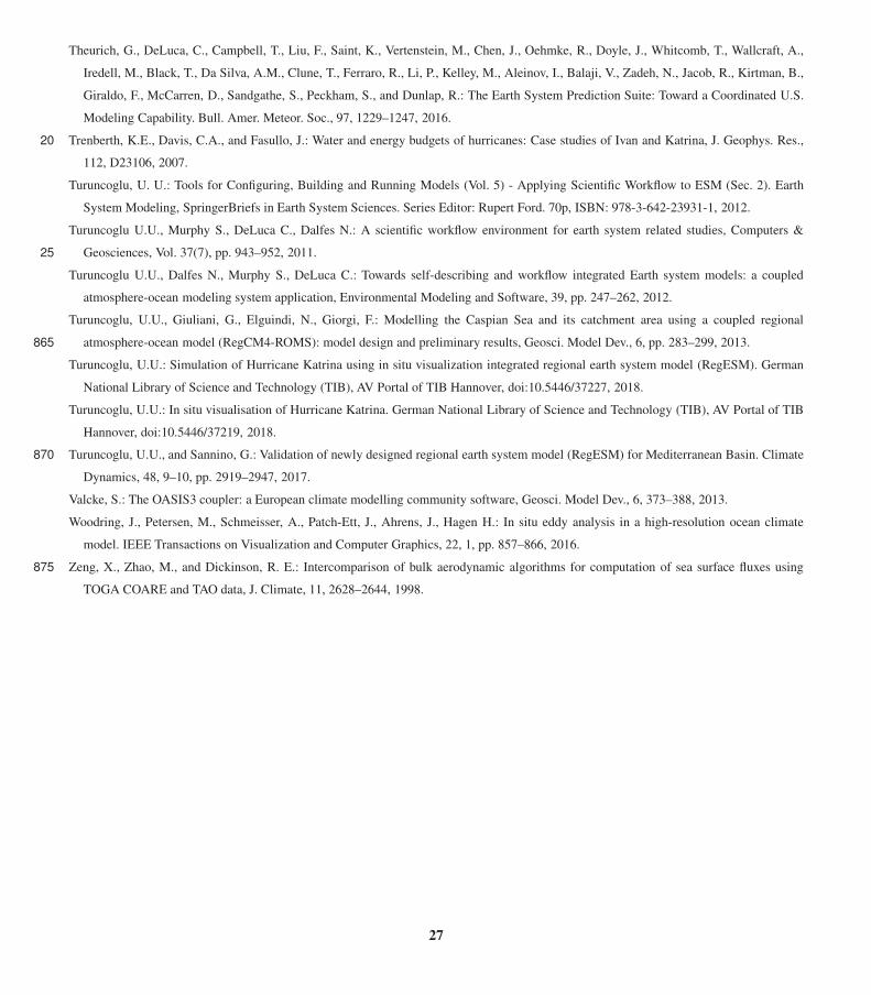
Theurich, G., DeLuca, C., Campbell, T., Liu, F., Saint, K., Vertenstein, M., Chen, J., Oehmke, R., Doyle, J., Whitcomb, T., Wallcraft, A.,

Iredell, M., Black, T., Da Silva, A.M., Clune, T., Ferraro, R., Li, P., Kelley, M., Aleinov, I., Balaji, V., Zadeh, N., Jacob, R., Kirtman, B.,

Giraldo, F., McCarren, D., Sandgathe, S., Peckham, S., and Dunlap, R.: The Earth System Prediction Suite: Toward a Coordinated U.S.

Modeling Capability. Bull. Amer. Meteor. Soc., 97, 1229–1247, 2016.

Trenberth, K.E., Davis, C.A., and Fasullo, J.: Water and energy budgets of hurricanes: Case studies of Ivan and Katrina, J. Geophys. Res.,20

112, D23106, 2007.

Turuncoglu, U. U.: Tools for Configuring, Building and Running Models (Vol. 5) - Applying Scientific Workflow to ESM (Sec. 2). Earth

System Modeling, SpringerBriefs in Earth System Sciences. Series Editor: Rupert Ford. 70p, ISBN: 978-3-642-23931-1, 2012.

Turuncoglu U.U., Murphy S., DeLuca C., Dalfes N.: A scientific workflow environment for earth system related studies, Computers &

Geosciences, Vol. 37(7), pp. 943–952, 2011.25

Turuncoglu U.U., Dalfes N., Murphy S., DeLuca C.: Towards self-describing and workflow integrated Earth system models: a coupled

atmosphere-ocean modeling system application, Environmental Modeling and Software, 39, pp. 247–262, 2012.

Turuncoglu, U.U., Giuliani, G., Elguindi, N., Giorgi, F.: Modelling the Caspian Sea and its catchment area using a coupled regional

atmosphere-ocean model (RegCM4-ROMS): model design and preliminary results, Geosci. Model Dev., 6, pp. 283–299, 2013.865

Turuncoglu, U.U.: Simulation of Hurricane Katrina using in situ visualization integrated regional earth system model (RegESM). German

National Library of Science and Technology (TIB), AV Portal of TIB Hannover, doi:10.5446/37227, 2018.

Turuncoglu, U.U.: In situ visualisation of Hurricane Katrina. German National Library of Science and Technology (TIB), AV Portal of TIB

Hannover, doi:10.5446/37219, 2018.

Turuncoglu, U.U., and Sannino, G.: Validation of newly designed regional earth system model (RegESM) for Mediterranean Basin. Climate870

Dynamics, 48, 9–10, pp. 2919–2947, 2017.

Valcke, S.: The OASIS3 coupler: a European climate modelling community software, Geosci. Model Dev., 6, 373–388, 2013.

Woodring, J., Petersen, M., Schmeisser, A., Patch-Ett, J., Ahrens, J., Hagen H.: In situ eddy analysis in a high-resolution ocean climate

model. IEEE Transactions on Visualization and Computer Graphics, 22, 1, pp. 857–866, 2016.

Zeng, X., Zhao, M., and Dickinson, R. E.: Intercomparison of bulk aerodynamic algorithms for computation of sea surface fluxes using875

TOGA COARE and TAO data, J. Climate, 11, 2628–2644, 1998.

27

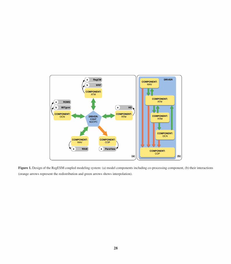
Figure 1. Design of the RegESM coupled modeling system: (a) model components including co-processing component, (b) their interactions

(orange arrows represent the redistribution and green arrows shows interpolation).

28

ATM

OCN

RTM

AT

M-O

CN

OC

N-A

TM

co

up

lin

g t

ime

AT

M-R

TM

RT

M-O

CN

co

up

lin

g t

ime

AT

M-O

CN

OC

N-A

TM

co

up

lin

g t

ime

AT

M-O

CN

OC

N-A

TM

co

up

lin

g t

ime

AT

M-O

CN

OC

N-A

TM

co

up

lin

g t

ime

AT

M-O

CN

OC

N-A

TM

co

up

lin

g t

ime

AT

M-R

TM

RT

M-O

CN

co

up

lin

g t

ime

AT

M-O

CN

OC

N-A

TM

co

up

lin

g t

ime

Model Components3h 1dfast time step slow time step

t=0h t=3h ... t=21h t=24h t=27h ... t=45h t=48h ...

Initialization

of models

WAV

AT

M-W

AV

WA

V-A

TM

co

up

lin

g t

ime

AT

M-W

AV

WA

V-A

TM

co

up

lin

g t

ime

AT

M-W

AV

WA

V-A

TM

co

up

lin

g t

ime

AT

M-W

AV

WA

V-A

TM

co

up

lin

g t

ime

AT

M-W

AV

WA

V-A

TM

co

up

lin

g t

ime

AT

M-W

AV

WA

V-A

TM

co

up

lin

g t

ime

Explicit Type Coupling

Figure 2. The run sequence of model components in case of explicit type coupling. In this case, the fast coupling time step is used for the

interaction between the atmosphere, ocean and wave components. The slow coupling time step is only used to interact with the river routing

component.

29

Figure 3. Schematic representation of (a) explicit and (b) semi-implicit model coupling between two model components (atmosphere and

ocean). The numbers indicate the execution orders, which is initialized in each coupling interval.

30

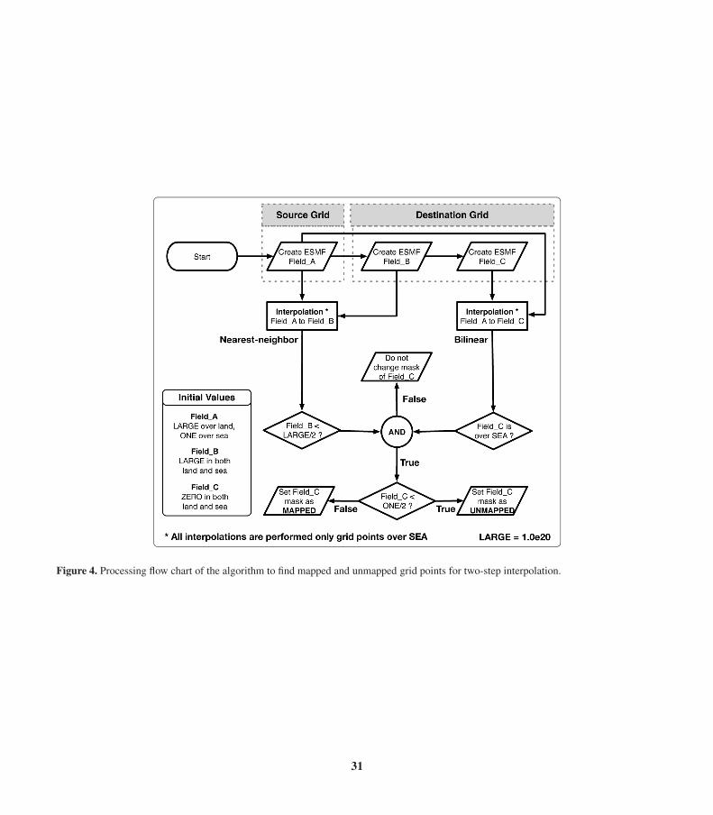
Figure 4. Processing flow chart of the algorithm to find mapped and unmapped grid points for two-step interpolation.

31

Simulation Code

Adaptor

Catalyst

Visualization Pipeline, Python Script

Rendered Image/s

Field Data

Analysis Result/s

Code A Catalyst

Visualization Pipeline, Python Script

Code B

Code C Code D

ESMFDriver

Adaptor

Paraview

Paraview

Statistics

Rendered Image/s

Field Data

Analysis Result/s

Statistics

(a)

(b)

Figure 5. Comparison of the (a) conventional and (b) ESMF integrated in-situ visualization system.

32

Initialize

CoProcess

Finalize

time stepping loop

if co-processing

ends

Initialize

Run

Finalize

Co-processing Component(ParaView, Catalyst)

The driver - RegESM(ESMF, NUOPC)

2

3 1

5

6 4

7 8

transfer

component grids

and field information

define

grids and fields

run

models and

connectors

redistribute field data

to co-processing

if simulation

ends

initialize individual

model components

and driver

run

Figure 6. The interaction between driver defined by ESMF, NUOPC and co-processing component (Paraview, Catalyst).

33

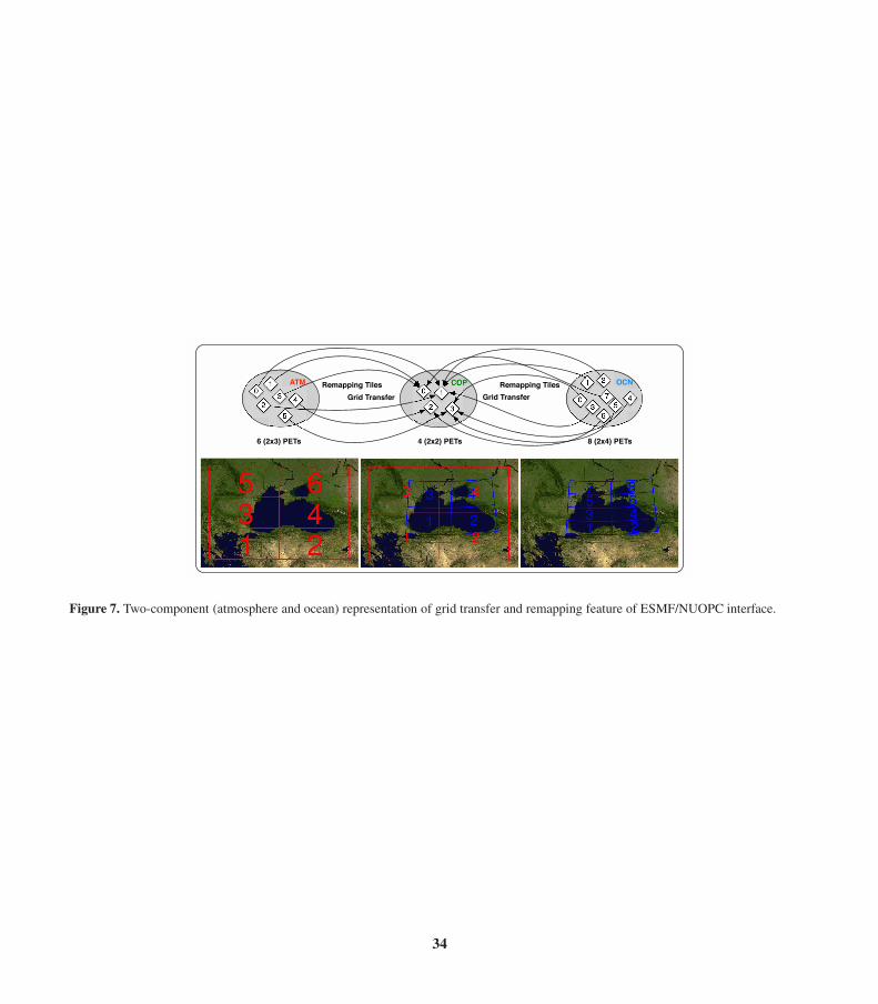
0

2

1

3

5

4 0

3

1

7

6

5

4

2

0

2

1

3

ATM OCNCOPRemapping Tiles

Grid Transfer

6 (2x3) PETs 8 (2x4) PETs4 (2x2) PETs

Remapping Tiles

Grid Transfer

Figure 7. Two-component (atmosphere and ocean) representation of grid transfer and remapping feature of ESMF/NUOPC interface.

34

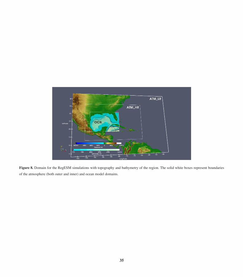
Figure 8. Domain for the RegESM simulations with topography and bathymetry of the region. The solid white boxes represent boundaries

of the atmosphere (both outer and inner) and ocean model domains.

35

Table 1. Tested model configurations for benchmark simulations. Note that the dimension of vertical coordinates of ATM and OCN compo-

nents are shown here after vertical interpolation from sigma to height and s-coordinates to depth.

P1: Case I P2: Case II P3: Case III

Visualization

Pipeline

Primitives ATM: Contour for

topography polyline

for coastline and direct

volume rendering for

clouds

ATM: same with pre-

vious case but it in-

cludes iso-surface for

wind speed and glyph

for wind at specified

level

ATM: Contour for

topography, iso-surface

for wind speed colored

by relative humidity

OCN: Contour for

bathymetry, direct

volume rendering for

current

Domain Size ATM

LR: 170 x 235 x 27

HR: 880 x 1240 x 27

ATM

Same with Case I

ATM

Same with Case I

OCN

653 x 487 x 21

Number of Fields 1 x 3D ATM

Relative Humidity

4 x 3D ATM

Relative Humidity

Wind (u, v, w)

4 x 3D ATM

Relative Humidity

Wind (u, v, w)

4 x 3D OCN

Ocean Current (u, v, w)

Land-Sea Mask

Data Size

ATM+OCN (MB)

LR: 8.3

HR: 224.0

LR: 33.2

HR: 896.0

LR: 33.2+25.4 = 58.6

HR: 896.0+25.4 = 921.4

Time (s) LR: 2.3 – 3.7

HR: 17.7 – 65.0

LR: 2.3 – 3.8

HR: 18.4 – 79.3

LR: 6.8 – 14.6

HR: 7.8 – 10.1

36

(a)

(b)

Figure 9. Benchmark results of standalone (a) atmosphere (ATM; both LR and HR) and (b) ocean (OCN) models. Note that timing results

of the atmosphere model is in log axes to show both LR and HR cases in the same figure. The black lines represent measured wall clock

times in second and red lines (and shaded envelope) show speed-up. The best two-dimensional decomposition parameters, timing results,

and speed-up are shown as a line for the ocean model case.

37

Figure 10. Benchmark results of (a) CPL simulations (b) COP simulations with P1 visualization pipeline, (c) COP simulations with P2

visualization pipeline and (d) COP simulations with P3 visualization pipeline. CPL represents the two-component modeling system (ATM

and OCN), and COP indicates three-component modeling system (ATM, OCN and co-processing). Note that the HR case requires at least

140 cores to run and the speed-up results are given based on 140 cores.38

Figure 11. Volume rendering of atmospheric relative humidity field (atm_input3d) as well as vorticity field in the ocean surface (ocn_input2d)

from COP_LR simulation using ParaView Catalyst in live mode.

39

Figure 12. Rendering of multi-component (ATM-OCN-COP) fully coupled simulation using ParaView. The temporal interval for the pro-

cessed data is defined as 6-minutes.

40

Figure 13. Rendering of three-dimensional vorticity streamlines (s−1), total precipitation (mmday−1) and sea surface temperature anomaly

(degC) of COP_LR simulation for 28-Aug-2005 00:00 UTC (a-c) and 29-Aug-2005 00:00 UTC (d-f). Streamlines are calculated only from

the eye of the hurricane. In this case, red and yellow colored forward streamlines represent cloud liquid water content (kgkg−1), and blue

colored backward streamlines indicate wind speed (ms−1). The solid yellow line represents the best track of Hurricane Katrina, which is

extracted from HURDAT2 database.

41

Figure 14. Same with Fig. 13 but for COP_HR simulation. The comparison of low and high-resolution model results is shown in the

supplemental video.

42