Towards an overview of spatial up-conversion techniques

Meng Zhao*, Jorge A. Leitao*and Gerard de Haan+**Eindhoven University of Technology, The Netherlands

+Philips Research Laboratories Eindhoven, The Netherlands

m.zhao@tue.nl

Abstract: The introduction of High definition television (HDTV) asks for spatial up-conversion techniques enabling the display of standard definition material (SDTV). The paper provides an overview of some important linear and non-linear methods. We further include a performance evaluation using a Mean Square Error criterion and show relevant screen shots to allow for a subjective impression obtained with the described algorithms.

Keywords: Image enhancement, spatial up-conversion, up-scaling

1. Introduction The advent of HDTV emphasizes the need for

spatial up-conversion techniques that enable standard definition (SD) video material to be viewed on high definition (HD) television (TV) displays. Conventional techniques are linear interpolation methods such as bilinear interpolation and methods using poly-phase low-pass interpolation filters. The former is not popular in television applications because of its low quality, but the latter is available in commercially available ICs, like [1]. With the linear methods, the number of pixels in the frame is increased, but the high frequency part of the spectrum is not extended, i.e. the perceived sharpness of the image is not increased. In other words, the quality of the display is not fully exploited. To solve this problem, LTI (Luminance Transition Improvement) after linear up-conversion and many non-linear up-conversion techniques have been proposed [7]. The class of non-linear methods can be divided

into directional interpolation methods and classification based methods. The former interpolates the pixels using edge information. The aim is to avoid interpolation across the edge, which would cause the result image to appear blurred. The directional interpolation methods include ELA (Edge-directed Line Averaging) [2], which has been designed mainly for de-interlacing purpose, and NEDI (edge-directed interpolation) [3], which was intended for image scaling. The content-based (or classification based) interpolation methods include DRC 1

1What we describe as Digital Reality Creation (DRC) is the

method revealed in US-patent 5,444,487, [5]. We believe

(Digital Reality Creation) [4] and RS (Resolution Synthesis) [5], which are quite similar techniques that differ only in their classification method. We have chosen DRC to represent the content-based techniques, because it has been introduced in television sets on the consumer electronics market.

To enable a comparison of the mentioned spatial up-conversion methods, we first down-sample the input image or the video sequence by a factor of four, and then up-scale it to the original size. Finally, we compare the up-scaled result with the original one, using an objective quality metric, the MSE (Mean Square Error).

The remainder of the paper is organized as follows. In section 2, we will briefly present the evaluated up-conversion algorithms. The actual evaluation is given in Section 3. Finally, in section 4, we draw our conclusions.

2. Advanced up-conversion algorithms

In this Section, we shall give a brief introduction to each non-linear up-conversion techniques to be covered in our evaluation. A. DRC

+'�9LGHR6LJQDO

/3)'RZQ�

VDPSOLQJ6'�9LGHR�6LJQDO

$'5&

/87�RI�,QWHUSRODWLRQFRHIILFLHQW

&ODVVFRGH

/HDVW�6TXDUH0HWKRG

)+'

)6'

Fig. 1. The learning process in DRC

“DRC” is commonly used to refer to this method, although the patent does not mention this name.

Basically, DRC is a data dependent interpolation filter [4]. The momentary filter coefficients, during interpolation, depend on the local (block) content of the image, which can be classified into classes based on the pattern of the block. To obtain the filter coefficients, a learning process should be performed in advance. Shown in Figure 1, the learning process employs both the HD-video and the SD video as the training material and uses the LMS (Least Square Method) algorithm to get the optimal coefficients. The training process is computational intensive due to the large number of classes. Fortunately it needs to be performed only once. In practical systems, classification of luminance blocks is realized by using ADRC (Adaptive Dynamic Range Coding) [6], which for 1-bit per pixel encoding reduces to:

≥<

=$96'

$96'

))))4 ��

��(1)

Here 6') is the luminance value of the SD pixel

and $9) is the average luminance value of the

pixels in the current aperture. 4 is the encoding result of ADRC. Other classification techniques can be thought of, the reason to use ADRC is its simple implementation. Using eq. (1), the number

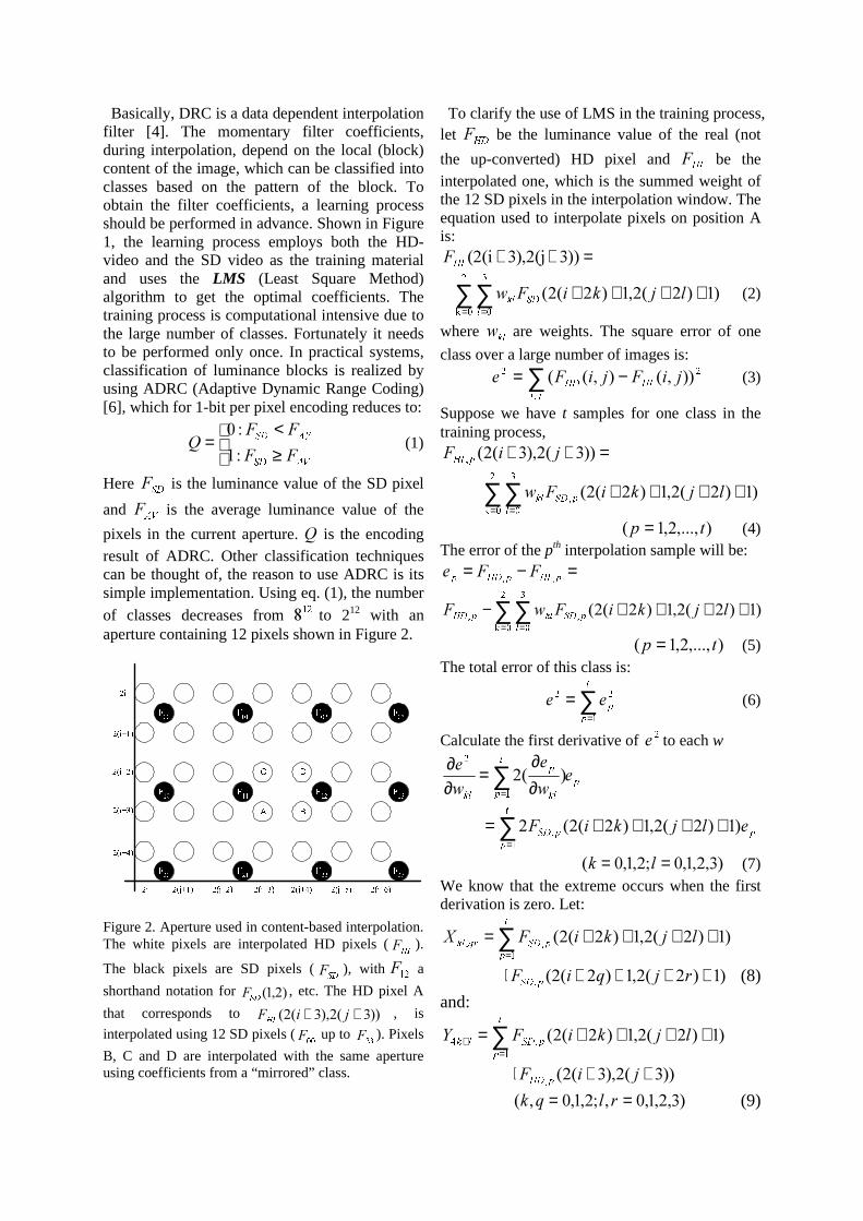
of classes decreases from ��� to 212 with an aperture containing 12 pixels shown in Figure 2.

'&

%$

)�� )�� )�� )��

)�� )�� )�� )��

)�� )�� )�� )��

�M ��M��� ��M���

�L

��L���

��L���

��L���

��L���

��M��� ��M��� ��M��� ��M���

Figure 2. Aperture used in content-based interpolation. The white pixels are interpolated HD pixels (

+,) ).

The black pixels are SD pixels (6') ), with ��) a

shorthand notation for �����6') , etc. The HD pixel A

that corresponds to ����������� ++ ML)+,, is

interpolated using 12 SD pixels (��) up to

��) ). Pixels

B, C and D are interpolated with the same aperture using coefficients from a “mirrored” class.

To clarify the use of LMS in the training process, let +') be the luminance value of the real (not

the up-converted) HD pixel and +,) be the interpolated one, which is the summed weight of the 12 SD pixels in the interpolation window. The equation used to interpolate pixels on position A is:

=++ ������M�����L+,)∑∑

= =

++++�

�N

�

�

�������������O

6'NO OMNL)Z (2)

where NOZ are weights. The square error of one

class over a large number of images is:

∑ −=ML

+,+' ML)ML)H�

�� �������� (3)

Suppose we have t samples for one class in the training process,

=++ ������������ ML) S+,

∑∑= =

++++�

�N

�

�� �������������

OS6'NO OMNL)Z

���������� WS = (4) The error of the pth interpolation sample will be:

=−= S+,S+'S ))H ��

∑∑= =

++++−�

�N

�

��� �������������

OS6'NOS+' OMNL)Z)

���������� WS = (5) The total error of this class is:

∑=

=W

SSHH

�

�� (6)

Calculate the first derivative of �H to each w

S

W

S NO

S

NO

HZH

ZH ∑

= ∂∂

=∂∂

�

� ���

∑=

++++=W

SSS6' HOMNL)

�� ��������������

��������������� == ON (7) We know that the extreme occurs when the first derivation is zero. Let:

∑=

++++=W

SS6'TUNO OMNL);

��� �������������

�������������� ++++⋅ UMTL) S6' (8)

and:

∑=

+ ++++=W

SS6'ON OMNL)<

��� �������������

������������ ++⋅ ML) S+'

����������������� == UOTN (9)

We get:

=

��

�

�

�

��

��

��

��

���������������

���������������

���������������

���������������

<

<<<

Z

ZZZ

;;;

;;;;;;;;;

��

�

����

�

�

�

(10)

Solving eq. (10) for all classes, we obtain the coefficients NOZ . Once we have all the filter

coefficients, interpolation becomes a simple calculation using eq (2). B. NEDI The NEDI (New Edge-Directed interpolation)

method [3] is a non-iterative orientation-adaptive interpolation scheme for natural image sources. It aims at interpolating along edges rather than across them to prevent blurring. This method adapts the interpolation filter coefficients to the local image content. NEDI assumes that the edge orientation does not change with scaling, recognizing the resolution-invariant property of edge orientation. Therefore, the coefficients can be approximated from the low-resolution image within a local window by using the LMS method.

$

%

&)��)�� )�� )�� )�� )��

)��)�� )�� )�� )�� )��

)�� )�� )�� )�� )�� )��

)��)�� )�� )�� )�� )��

)�� )�� )�� )�� )�� )��

)�� )�� )�� )�� )�� )��

�L

��L���

�M ��M��� ��M��� ��M�����M��� ��M���

��L���

��L���

��L���

��L���

��L���

��L���

��L���

��L���

��L���

��M��� ��M��� ��M��� ��M��� ��M���

Figure 3. Aperture used in new edge-directed interpolation. A is the aperture with four SD pixels involved in interpolation. B is the aperture with the SD pixels used to calculate the four interpolation coefficients. C is the aperture that includes all the diagonal neighbours of the SD pixels in B. Here, ��) is

a shorthand notation for �����6') , etc.

NEDI uses a fourth order interpolation

algorithm

=++ ����������� ML)+,

∑∑= =

+ ++�

�

�

�� �������

N O6'ON OMNL)Z (11)

Denoting M as the pixel set used to calculate the four weights, the MSE over set M in the optimization can be written as:

=06(∑ ++−++ji

HIHD ML)ML),

2���������������� (12)

Which in matrix formulation becomes: �&Z\06( && −= (13)

Here, \& contains the pixels in M (pixel �����6')to �����6') , �����6') to �����6') , �����6') to

�����6') , �����6') to �����6') and C is a �� 0× matrix whose kth row is composed of the

4 diagonal neighbours of each value in \& .

To find the minimum MSE, the derivation of MSE over Z& is calculated:

�=∂

∂Z

06((14)

��� � =+− &Z&\ &&(15)

���� � \&&&Z 77 && −= (16)

In smooth areas ��� −&& 7 may not be fully

ranked, so there is no answer for Z& . Therefore, smooth-area detection is performed prior to the calculation and linear interpolation is used in these areas. C. ELA

6'�SL[HO�JULG+'�SL[HO�WR�EHLQWHUSRODWHG

��L���

�L

��L���

��M��� ��M��� �M ��M��� ��M���

D E F G H

Figure 4. The vertical aperture of Modified ELA The ELA (Edge-directed Line Averaging)

method is derived from the de-interlacing techniques. Although applicable to up-scaling, it has not been optimised for this function. The use of the modified ELA [2] method is limited to a smaller range of edge orientations. In detail, the modified ELA uses a directional correlation between the pixels (in white) in the adjacent original scan lines to determine the direction for interpolation. This is shown in Figure 5. In the

modified ELA method, directions a to e are detected. For spatial up-conversion, it first edge

dependently up-scales the SD image vertically to obtain an intermediate image ,0) :

��������������� K6',0 OML)ML) −−=

����������

K6' OML) +++ (17)

Thereafter, ,0) is up-scaled horizontally to obtain the HD image:

��������������� MOL)ML) Y,0+, −=+

���������� +++ MOL) Y,0 (18)

As before, ����� ML)+, is the HD luminance value

of a pixel in the image at position ����� ML[ =&.

Parameters YK OO � depend on the edge orientation.

3. Evaluation

To evaluate the described conversion methods,

we selected 5 SD video sequences. In order to enable an MSE calculation, for which we need a perfect HD reference, we first down-sample the video sequence by a factor of 4 and then up-scale it to the original size. We compared the original video sequences and their corresponding up-converted ones by using the MSE criterion. Figure 5 depicts the evaluation process.

+'�9LGHR6LJQDO

'RZQ�VDPSOLQJ

6'�9LGHR6LJQDO

'LIIHUHQW8S�&RQYHUVLRQ7HFKQLTXHV

+'�9LGHR6LJQDO

�5HFRQVWUXFWHG�

&RPSDULVRQDQG

&RQFOXVLRQFigure 5. Evaluation flowchart of various spatial up-conversion techniques

�D��/HQQD �E��7RN\R

�F��6LHQD �G��)RRWEDOO �H��%LF\FOH

Figure 7. Images from each test sequences

A Pre-processing From the descriptions in Section 2, we conclude

that different up-scaling methods result in different HD-pixel grids. For instance, the result of DRC is shifted over 0.5 pixel, while ELA and EDDI introduce no such shift. To cope with both options in a fair comparison, we produced two copies of the selected video sequences. The first is shifted over 0.25 pixel and the other over 0.75 pixel. This results in two “originals” on different grids that have the same picture quality. Shown in Figure 6, pixels on grid A are original

HD pixels, the other pixels are interpolated using a FIR interpolation filter. Pixels on grid B and C are one quarter and three quarter pixel shifted compare to A respectively. For DRC, the pixels are sitting on the same grid as the original after the processing. For other methods, there is half pixel shift after the processing.

$ $

% %

& &

$ $

% %

& &

$ $

$

$

$

Figure 6. Shift of the HD pixel grid B. The down sampling To avoid alias occur during down sampling, the

first choice is to use a low-pass anti-alias pre-filter before decimation. The result, however, is not an appropriate model for a picture from a low-resolution imaging device. A better approximation results, applying a Gaussian filter, i.e. to simply average the 4 pixels within each HD cell when emulating a SD-cell. Since a camera usually has an aperture correction filter to compensate for the roll-off characteristic in the high frequency part, it seems appropriate to include a peaking filter in the evaluation. What we used is a cascade of the 4-point averaging down-sampling:

=++ ������� ML)6'

∑∑= =

++�

�

�

�

�����������

N O+' OMNL) (19)

and a 3-tap peaking filter:

������������������

ML)ML)ML)ML)

6'6'

6'RXW

+−++−−=

ααα

(20)

here, ����=α gives the best result according to our experiment result. In eq.(20) we only define the vertical peaking filter, but the same filter is used in the horizontal domain. Down-sampling the original HD video with a 7-tap standard low-pass FIR filter2 is also presented as a reference in the evaluation. C. The up-conversion and MSE calculation After up-conversion of the down-sampled video

with a factor of 4, using the linear and non-linear methods, the MSE between the original video image(s) and the up-converted one(s) is calculated using:

∑ −=ML

) ML*ML)106(�

����������(21)

��� ML) and ��� ML*) are the luminance values of the original image and the up-converted one, respectively, while N represents the number of pixels in the image. The techniques that we evaluated are: $ ELOLQHDU�LQWHUSRODWLRQ��%,�� $ ���WDSV�LQWHUSRODWLRQ�ILOWHU��),5�3;7KH�PRGLILHG�(/$��(/$�� 7KH�'5&��&ODVVLILFDWLRQ�EDVHG�LQWHUSRODWLRQ��

The NEDI (New Edge Directed Interpolation); D. Results and comparison

��

����

���

��

����

���

��

���

�

��

��

��

��

���

���

���

���

*DXVVLDQ

),5

%, ),5 (/$ '5&1(',

Figure 8. Comparison of spatial up-scaling methods using the MSE criterion

2 This filter was standard Matlab decimation filter and had the following coefficients: -0.0087, 0, 0.2518, 0.5138, 0.2518, 0, -0.0087. 3 This filter was standard MatLab up-scaling filter and had the following coefficients: 0.0002, 0, -0.0017, 0, 0.0077, 0, -0.0251, 0, 0.0672, 0, -0.1693, 0, 0.6210, 1.0, 0.6210, 0, -0.1693, 0, 0.0672, 0, -0.0251, 0, 0.0077, 0, -0.0017, 0, 0.0002.

We used five test sequences for evaluation. There is a stationary image with many details (Lenna), a horizontally moving sequence with much vertical detail (Tokyo), a zooming scene with low contrast detail (Football), a vertically moving image with detailed lettering and fine structure (Siena), and a sequence with complex motion and high contrast diagonals (Bicycle). Figure 7 shows a picture from each test sequence. Figure 8 shows a comparison of the algorithms

using the MSE criterion. All methods show better MSE-scores with the down sampling using a Gaussian filter and aperture correction. The (long) FIR-filter interpolation shows the best MSE-score. The MSE-score of NEDI and DRC, is between that of the bi-linear method and the FIR-interpolator. The ELA scores clearly worst.

�D� �E�

�F� �G�

�H� �I�

Figure 9. Detailed area of different spatial up-scaling (a) Original picture, others are up-scaled using (b) bilinear interpolation, (c) FIR interpolation filter, (d) New-edge Directed Interpolation, (e) DRC, (f) Modified ELA. To enable a subjective impression, Figure 9

shows the detailed area of an original picture and its up-converted counterparts using different up-scaling algorithms. The modified ELA produces clear artefacts, particularly visible in the text area,

due to erroneous interpolation directions. We conclude that ELA seems unsuitable for up-scaling. The result of bilinear interpolation is rather blurred compared to the other methods. The FIR interpolation method visually performs well in fine structured areas, but along edges, overshoots are clearly visible. The DRC and NEDI methods yield less overshoot at the edges, but are somewhat weaker in fine structured areas.

4. Concluding remarks

We have presented an overview of spatial up-scaling techniques, including conventional linear methods, a 27-taps FIR-filter, and a bilinear interpolator, and some recently developed non-linear algorithms, like ELA, DRC and NEDI. From our evaluation, we conclude that NEDI and DRC visually perform well on edges, but are not as good as a conventional linear FIR-interpolator in fine structured areas. In terms of MSE-score, the FIR-filter performs best of all evaluated methods, although DRC and NEDI come close. References [1] GF9320 scaling processor, preliminary data sheet, Gennum, June 2001. [2] H. Lee et.al., ‘Adaptive scan rate up-conversion system based on human visual characteristics’. IEEE trans. on Consumer Electronics, Vol. 46, No. 4, Nov. 2000, pp. 999-1006. [3] X. Li et.al., ‘New edge-directed inter-polation’. IEEE trans. on Image Processing, Vol. 10, No 10, October 2001, pp. 1521-1527. [4] T. Kondo et.al., ‘Picture conversion appa-ratus, picture conversion method, learning apparatus and learning method’, Sony corp., US-patent 6,323,905. [5] C. B. Atkins et. al., ‘Optimal image scaling using pixel classification’, 2001 International Conference on Image Processing, Volume 2, 2001, vol.3, pp864-867. [6] T. Kondo et.al., ‘Adaptive dynamic range encoding method and apparatus’, Sony corp., US-patent 5,444,487. [7] P. Rieder et. al., ‘New concept on denoising and sharpening of video signals’, IEEE Trans. on Consumer Electronics, vol.47, No.3, pp666-671, Aug. 2001.