Towards A Framework For Resilient Design OfComplex Engineered Systems

As modern systems continue to increase in size and complex-ity, they pose significant safety and risk management chal-lenges. System engineers and much of the government re-search efforts are focused on understanding the attributesand characteristics that emerge from the interactions of com-ponents and subsystems. As a result, the objective of thisresearch is to develop techniques and supporting tools forthe verification of the resilience of complex engineered sys-tems during the early design stages. Specifically, this workfocuses on automating the verification of safety requirementsto ensure designs are safe, automating the analysis of de-sign topology to increase design robustness against inter-nal failures or external attacks, and allocating appropriatelevel of redundancy into the design to ensure designs areresilient. In distributed complex systems, a single initiat-ing fault can propagate throughout engineering systems un-controllably, resulting in severely degraded performance orcomplete failure. This research is motivated by the fact thatthere is no formal means to verify the safety and resilienceproperties, and no provision to incorporate related analysisinto the design process. The proposed approach is validatedon the quad-redundant Electro-Mechanical Actuator (EMA)of a Flight Control Surface (FCS) of an aircraft.

1 IntroductionIn recent years, technological advancements and a grow-

ing demand for highly reliable complex engineered systems,e.g., aviation, power generation, transportation, and healthcare have made the safety assessment of these systems evermore important [1, 2]. These systems are considered safety-critical and are required to perform more reliably in dynami-cally uncertain operational environments. Consequently, thedevelopment of systems with broader fault detection and di-agnosis capabilities is vital for protecting lives, property, andcontinuity of service. Looking back at the Columbia spaceshuttle incident of 2003, it is evident that the illogical pursuitof the design mantra of better, cheaper, faster led to the de-cisions that eroded safety without realizing that the risks haddramatically increased. In the aftermath of such catastrophicfailure and similar major accidents, it has become apparentthat complex systems design and development require bothultra-high safety and high performance [3].

In order to design a resilient system, first we define theconcept of complex systems. System of systems (SOS) isa collection of other elements which themselves are distinctcomplex systems that interact with one another to achievea common goal. The more the number of systems, the

higher the possibility of negative interaction occurrence, thatis emergence. The reason for this is that (1) the systems con-stituting the SOS were designed independently and were notoriginally designed to work together, and (2) each system inthe SOS may be of a different technology.

The SOS performs functions and achieves results thatcan not be achieved by any specific component. More pre-cisely, the performed functions are characterized by the be-haviors that are emergent properties of the entire SOS and notthe behavior of any specific system component. Paries [4],Bedau [5], Chalmers [6], and Seager [7] categorized theseemergent properties into three distinct types: (1) normalemergence, (2) weak emergence, and (3) strong emergence.

The three categories of emergence are depicted in Fig-ure 1. According to Bedau and Chalmers [5, 6], normalemergence is a system property, which results from multi-ple components or sub-systems working together to performa required function. Hence, normal emergence is a desirablesystem behavior, while weak and strong emergence are con-sidered undesirable and possibly catastrophic types of emer-gence. Pavard et al. [8] looks at an air traffic control systemas a good example of normal emergence. In this system,a specific and fixed role is assigned to Flight ManagementSystem (FMS), Instrument Landing System (ILS), and theair traffic controller. The function of a designed system withnormal emergence is an intended emergent property of theplanned interaction of the individual parts and components.

On the other hand, weak emergence is defined as anemergence that could be predicted and prevented if all thelaws of physics are taken into the consideration and exhaus-tive simulation and verification is conducted. One exampleof weak emergence is the Mars Polar Lander as explained byLeveson [9]. In this accident, the Lander strut vibration wasinterpreted by software as a landing signal. Therefore, soft-ware shut down both engines, and the lander crashed intothe planet. If the system, including software, physical sys-tem, and their interactions had been verified properly withexhaustive simulation of the vibration of the strut, then thecatastrophic failure might never have happened.

Lastly, strong emergence is one of the most difficulttypes of emergence to be identified. By nature, this type ofemergence results from completely random factors and itssource is often human. The Nagoya incident as describedby Leveson [10] is one example of strong emergence. Inthis case, the pilot mistakenly sent a wrong command to theflight control system, which resulted in loss of passengers’and pilot’s life. The important question to ask here is how the

1 INTRODUCTION 2

Possible to predict if all the laws of physics are studied and analyzed

Impossible to predict.(Causes are completely random)

System of Systems (Complex Systems)

Minimize the consequences of failures

Normal Emergence Weak Emergence Strong Emergence

Recover from Failures

Resilient System

predicts and prevents functional losses and disruptions

Fig. 1: Resilience and Emergence in Systems.

Verification Stage

State of the Art

Reliability-based Hazard-based

Design Stage

Verification Stage

Design Stage

Reliability Block

Diagrams(RBD)

Failure Modes and

Effects Analysis(FMEA)

Function Failure Design Method(FFDM)

Risk in Early

Design(RED)

Function Failure

Identification & Propagation

(FFIP)

Fault Tree

Analysis(FTA)

Probabilistic Risk

Assessment(PRA)

Hazard and

Operability Studies

(HAZOP)

Systems-Theoretic Accident Modeling

and Processes(STAMP)

Fig. 2: Techniques for Safety and Reliability Analysis of System Design.

entire system, including aircraft and pilot could have beenmore resilient and adaptable to a range of external and inter-nal threats and failures.

In this paper, resilience is viewed as a system’s abilityto cope with complexity [11] and adapt to changes causedby emergence, either weak or strong. As depicted in Fig-ure 1, resilience is characterized as a multi-faceted propertyof complex systems that (i) predicts and prevents functionallosses and disruptions, (ii) minimizes the impact of failures,and (iii) recovers from disturbances. The result of this re-search provides a basis for incorporating risks into the designprocess of engineered systems and tools that proactively cap-ture how the internal system’s interactions and environmen-tal factors affect system resilience. In particular, this pro-

posal addresses the following three objectives

1. Failure prevention in system design through effectiveanticipation of disruption based on exhaustive simula-tion and verification of safety requirements.

2. Reduction of adverse consequences through identifica-tion of a design topology and physical system infras-tructure that is more robust against failures.

3. Recovery from disturbance through component redun-dancies while determining the least number of compo-nent redundancies that are required to tolerate and pre-vent catastrophic system failure.

The remainder of this paper is structured as follows: sec-tion 2 presents the background and related research on failure

2 BACKGROUND 3

analysis techniques in the early stages of system design. Insection 3 an overview of the step-by-step implementation ofthe framework, both at the component and system level, isexplained. Section 4 outlines the application of the proposedmethodology in the analysis and verification of the safetyproperties of the quad-redundant Electro Mechanical Actu-ator (EMA) system design. The paper ends with conclusionsand future work.

2 BackgroundA number of failure analysis techniques have been de-

veloped over the years. This section reviews several of thesecommon approaches for failure and reliability analysis dur-ing conceptual design of engineered systems. As depictedin Figure. 2, two distinct categories of methods are usu-ally adopted to address safety analysis of system design.First, reliability-based approaches are based on identifyingfault and their likelihood of occurring throughout the sys-tem life-cycle. The second category of techniques is basedon undesirable system states and focus on identifying pathsthat reach that state and the likelihood of that path. Hence,hazard-based techniques are system state centric whereas thereliability-based approaches are fault centric.

2.1 Reliability-based TechniquesThis work explores the reliability-based and hazard-

based perspectives and incorporates them into the conceptsof emergence and resilience as a groundwork for establish-ing a framework to evaluate the balance between the two ar-eas of risk mitigation. The following section will detail thetraditional approach to system design to provide the contextof this work.

2.1.1 Verification Stage ApproachesThis group of reliability analysis methods is based on the

symbolic logic of the conceptual models of failure scenarioswithin a design. The goal is to assess the probability of fail-ure occurrence in the system design. One of these methodsis the Reliability Block Diagram (RBD) [12], which dividesthe system into elements based on the functional model ofthe system design, where each system element is assigned areliability factor. Then a block diagram of the elements in aparallel, series, or the combination of parallel and series isconstructed. Each block represents a function or an event inthe system and each element’s failure mode is assumed in-dependent from the rest of the system. The reliability factormay or may not be available for all the system design ele-ments and should be assigned by an expert, which makes itsubjective and hard to validate.

The second popular method of reliability analysis, Fail-ure Mode and Effect Analysis (FMEA) [13] is a bottom upapproach that investigates failure modes of components andtheir effects on the rest of the system. In practice, this tech-nique is supported by a top-down analysis to confirm the an-alytical resolution. FMEA provides an exhaustive analysisto identify the single point of failures and their effects onthe rest of the system. The result of the analysis is used toincrease reliability, incorporate mitigation into the design,and optimize the design. However, FMEA is very costly

in terms of resources, particularly when implemented at thecomponent level within complex systems. Also, occurrencesof simultaneous failures and multiple faults are not evalu-ated. The completeness and correctness of the analysis isvery much dependent on the expert knowledge.

2.1.2 Design Stage ApproachesThe next category of reliability analysis techniques uses

functional modeling to represent the system design for anal-ysis. The Function Failure Design Method (FFDM) intro-duced by Stone et al. [14,15] is an example of such a method.FFDM can be used not only at the early stage of system de-sign but throughout the design process by creating a relation-ship between system functionality to failure modes and prod-uct function to system design concepts. Risk in Early Design(RED) method presented by Grantham et al. [16, 17] is builtupon the FFDM technique which formulates the functional-failure likeliness and consequence associated with each func-tion failure. Nevertheless, Devendorf [18] attests that REDis not able to assist the designers in effective error proofingduring the design process. The knowledge-based repositoryused by RED to provide relative failure information does notscale to other syntax.

In order to overcome these limitations, other researchefforts have drawn attention to the importance of failure cas-cades in reliability analysis. Kurtoglu at al. [19] presentedthe Function-Failure Identification and Propagation (FFIP)approach for detecting functional failure during the earlystages of system design by interleaving failure identificationanalysis with model based reasoning.

2.2 Hazard-based TechniquesHazard-based methodologies focus on system transi-

tions which move from a hazardous state to a failure statebased on a set of initiating mechanisms. Therefore, the aimof hazard-based techniques is to identify the potential haz-ards and the mechanisms and sequences of events which cancause the system to transition to a failure state in the presenceof those hazards.

2.2.1 Verification Stage ApproachesAnother symbolic logic model is based on the Fault Tree

Analysis (FTA) [20] which studies the failure propagationpath from the point of start to the vulnerable componentsand assigns a severity factor to each failure model. One ofthe benefits of using FTA is its ability to analyze the proba-bility of simultaneous occurrence of failure within a complexsystems. On the other hand, the probabilistic evaluation ofcomplex large systems could get computationally intensive.

Also, the correct probabilistic evaluation requires a sig-nificant amount of resources. Another form of symboliclogic modeling technique is known as Event Tree Analysis(ETA) [21] which differs from FTA analysis in a manner thatcovers both success and failure events. In this technique alltypes of events, such as nominal system operations, faultyoperations, and intended emerging behaviors, are modeled.Still, calculating the probability of non-comparative failureor success is difficult to estimate and reach agreement on.

Probabilistic Risk Assessment (PRA) [22] is a technique

3 METHODOLOGY 4

used for analysis of failure risk [23]. PRA incorporates anumber of fault/event modeling methods, such as event se-quence diagrams and fault trees, and integrates them into aprobabilistic analysis to guide decision-making during ver-ification stage. However, the requirement for developing afully specified system model as part of the verification pro-cess is constable. The reason is that such detailed, high-fidelity models of complex systems are not available duringearly stages.

2.2.2 Design Stage ApproachesAnother technique for safety analysis is Hazard and Op-

erability Studies (HAZOP) [24] that is based on modelingthe interaction flow between components and recognizing ahazard if components deviate from the intended operationof designs. A set of guidewords are provided to help withidentification of such deviations. However, from the contextof safety analysis based on interaction between componentsand their intended environments, HAZOP is unable to pro-duce repeatable hazard analysis of the same accident. Thereason for this weakness lies in the highly dynamic and un-predictable nature of interactions between different subsys-tems and their operational environment. Moreover, depend-ing on the expertise and skills of the safety engineers, thedeviations can be identified differently.

In systematic models, such as Systems-Theoretic Ac-cident Modeling and Processes (STAMP), accidents resultfrom several causal factors that occur unexpectedly in a spe-cific time and space [25]. Therefore, the system under con-sideration is not viewed as a static entity but as a dynamicprocess that is constantly adapting to achieve its goals andreacting to internal and environmental changes.

There are many benefits in using STAMP models as thebasis for hazard analysis of a complex system. However,Johnson et al. [26] state that the STAMP approach has twofundamental weaknesses: the lack of methodological guide-line in implementing the constraint flaw taxonomy and theconstruction of control models in a complex system is com-plicated. In addition, [26] presents two independent stud-ies of implementing STAMP hazard analysis techniques onthe mission interruption of the joint European Space Agency(ESA) and National Aeronautics and Space Administration(NASA) Solar and Heliocentric Observatory (SOHO). Thehazard analysis from each study resulted in significantly dif-ferent conclusions regarding the cause of failure in the sys-tem under study.

3 MethodologyThe techniques reviewed in the previous section are de-

signed to evaluate a limited set of scenarios in order todeal with the system complexity. The effects of this in-formal and incomplete verification is the possibility that anon-tested scenario could result in unexpected behavior andcatastrophic system failure. To address the incomplete veri-fication of designs via simulation, formal methods have beenproposed to increase the confidence level. Formal verifi-cation enables the evaluation of safety properties at differ-ent levels of abstractions,( i.e., component, sub-system, sys-

tem), proving that the system under consideration satisfies itssafety requirements.

The proposed framework relies on constructing a finitemodel of a design and checking it against its desired safetyproperties. In the context of this work, the properties of asystem are modeled as transition systems. A desired safetyproperty contains no failure states. In modeling and rea-soning about complex systems, it is more efficient to de-fine safety properties by directly declaring the desired be-havior of a system instead of stating the characteristics of afaulty behavior. Another advantage of modeling the systemas a finite-state machine and the fact that it is finite makes itpossible to execute an exhaustive state-space exploration toprove that the design satisfies its requirements. Since thereis an exponential relationship between the number of statesin the model and number of components that make up thesystem, the compositional reasoning approach [27] is usedto handle the large state-space problem. The compositionalreasoning technique decomposes the safety properties of thesystem into local properties of its components. These lo-cal properties are subsequently verified for each component.The combination of these simpler and more specific verifi-cations guarantee the satisfaction of the global safety of theoverall system architecture design. It is important to notethat, the safety requirements of the components are satisfiedonly when explicit assumptions are made on their environ-ment. Therefore, an assume-guarantee [28–32] approach isutilized to model each component with regards to its inter-action with its environment, i.e, the rest of the system andoutside world.

Next in the proposed framework, each design is con-verted to system-level graph representation. These graphrepresentations are then used as a tool to convert each de-sign into an adjacency matrix of nodes (components) andedge connections [33]. Subsequently, Non-Linear Dynam-ical System (NLDS) and epidemic spreading algorithms areused to analyze the propagation of failure in complex engi-neered system design.

Furthermore, the framework addresses the issue of for-mally specifying and formulating the design architecture thatis resilient to component failures by exploiting redundancy.The application of component redundancy improves systemreliability but also adds cost, weight, size, and power con-sumption. Therefore, it is vital to minimize the number ofredundancies. The safety analysis and verification processproposed in this research examines the number of choicesto determine a best way to incorporate redundancy into thedesign.

The proposed framework integrates safety by planningand anticipating for unexpected failures and disruptions.From this perspective, safety is considered a dynamic fea-ture of the system that requires constant reinforcement andsupport on an ongoing basis. It is important to recognizethat safety is a feature that results from what a system does,rather than a characteristic that a system has. Therefore, theproof of safety is only conveyed by the absence of failuresand accidents. For this reason, safety-proofing a system de-sign is never absolute or complete. However, in this research,

3 METHODOLOGY 5

Design Concepts

Learning Algorithm

Design Meets Safety Requirements

Complex Network

Failure Impact Analysis

Semi-Formal and Formal Verification

H61

Engineering Targets

Application of Component Redundancy

Resilient System Design

Minimize the effect of adverse consequences

Failure prediction & prevention

Recover from adverse consequences

Framework For Assessing And Improving The Resilience Of Complex Engineering Systems

Model Checking

0111

1011

1101

1110

Design Matrix

Markov Chain

)(ti )( 1 t

i

Epidemic Spreading

Fig. 3: An Overview of The Proposed Approach.

the proposed framework biases the odds in the direction thatensures safe system operation by 1- Predicting and prevent-ing adverse consequence 2- Minimizing the adverse con-sequences, and 3- Recovering from adverse consequences.Fig. 3 represents an overview of the approach which will bediscussed in detail in the next section.

3.1 Formal and Semi-Formal Verification ApproachesDesign requirements are the specification of safety con-

straints initially defined in the design [34]. Requirements aremodeled at different levels of abstractions. For example, ahigher level of abstraction is used when expressing the globalsystem properties and a low level of abstraction is used whenexpressing the required features for each system component,

Fig. 4: Requirements Decomposition.

3 METHODOLOGY 6

i.e. the barriers and materials to be used. Managing thisset of specifications is based on iterative decomposition andsubstitution of the abstract requirements by the requirementsthat are more concrete.

3.1.1 Safety Requirements Modeling Using SysMLTraditional methods and tools used by system engineer-

ing are mostly based on a formalism that capture a varietyof system features, i.e., requirements engineering, behav-ioral, functional, and structural modeling, etc. Those withparticular focus on requirements engineering are the UnifiedModeling Language (UML) [35] to support various aspect ofsystem modeling, Rational Doors [36] to express the require-ments, and Reqtify [37] to trace the requirements through de-sign and implementation. UML is developed by the ObjectManagement Group (OMG) in cooperation with the Interna-tional Council of Systems Engineering (INCOSE). UML isan Object-oriented modeling language that allows hierarchi-cal organization of system component models, which in turnresults in easier reuse and maintenance of the system model.However, UML was originally developed for software engi-neers and its primary application is software-oriented; there-fore it does not meet all the system engineers expectations.For example, UML does not provide a notion to representcontinuous flows exchanged within the system, i.e., Energy,Material, and Signal (EMS). The analysis of EMS flows arecrucial in system design safety verification for identifying thefailure propagation path and identifying the common failuremodes. For this reason, the SysML [38] profile was devel-oped borrowing a subset of the UML language to meet therequirements of a general purposed language for system en-gineering.

A SysML requirement diagram enables the transforma-tion of text-based requirements into the graphical modelingof the requirements which can be related to other modelingelements. Fig. 4 depicts the decomposition of a single ab-stract requirement into several more explicit ones. A studyby Blaise et al. [39] confirms the effectiveness of such di-agrams to facilitate the structuring and management of re-quirements that are traditionally expressed in natural lan-guages.

The next step in the requirement analysis phase consistsof mapping the requirements to the corresponding systemcomponents or functions. System components are modeledas part of the structural design of a system. The structural de-

sign model corresponds to the system hierarchy in terms ofsystems and subsystems, which are modeled using the BlockDefinition diagram (BDD). SysML blocks are the best mod-eling elements to model multi-disciplinary systems and areespecially effective during system specification and design.They are effective because blocks are not only able to modellogical or physical decomposition of a system, they also en-able designers to define specification of software, hardware,or human elements.

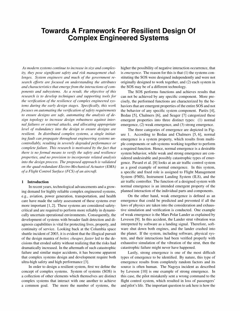
Fig. 5 illustrates how a single requirement can be satis-fied by a set of sub-systems and components. The require-ment diagram is connected to the structure diagram by across connecting element known as satisfy. A requirementcan be satisfied by a component or subsystem. Furthermore,the detailed modeling of sub-systems and components arepossible through the use of Internal Block Diagram (IBD).In addition, blocks are a reusable form of description thatcan be applied throughout the construction of system model-ing if necessary. Another advantage of using blocks duringthe design process is their ability to include both structuraland behavioral features, such as properties and operationsthat represent the state of the system and behavior that thesystem may display.

Including properties as part of the requirement model-ing is specifically important when verifying safety require-ments. As Madni. [40] demonstrated, safety is a changingcharacteristic of complex systems that, once integrated intothe design, is not preserved unless enforced throughout sys-tem operation. It is for this reason that in this paper safety isviewed as a system property.

A complete proof of safety is possible through a formaldefinition of different properties that are linked to each high-level abstract and low-level detailed requirements. Fig. 6 rep-resents how a requirement, property, block, and behavioralmodel are connected to one another. For example, allocateas a cross connecting principle in SysML is used to connecta behavior to a component in a structure diagram.

After decomposing safety properties of the system intolocal properties of its components. These local properties aresubsequently verified for each component. The combinationof these simpler and more specific verifications guaranteesthe satisfaction of the global safety of the overall system ar-chitecture design.

Fig. 5: Requirements Mapping.

3 METHODOLOGY 7

Fig. 6: Requirements Traceability.3.1.2 Automated Assume-guarantee Reasoning

In [41], Henzinger et al. cover the advantages that for-mal verification offers over the above approaches. In for-mal verification, system designers construct a precise math-ematical model of the system under design, so that exten-sive analysis is carried out to generate proof of correct-ness. One of the well-established methods for automaticformal verification of the system is model checking, wherea mathematical model of a system is constructed and veri-fied with regards to specified properties. In model check-ing, the desired properties are defined in terms of temporallogic, system of rules and symbolism for representing, andreasoning about, propositions qualified in terms of time [42].The defined logical formulae are then used to prove thata system design meets safety requirements and specifica-tions. A model checker to establish assume-guarantee prop-erties of components is called assume-guarantee reasoning(AGR) [43, 44]. In the assume-guarantee reasoning (AGR)method, the system properties are verified and modeled withrespect to the assumptions on the environment where com-ponent and (sub)system performances are guaranteed underthese assumptions. The assumption generation methodologyuses compositional and hierarchical reasoning approachesvia a compositional reachability analysis (CRA) [45] tech-nique. CRA incrementally composes and abstracts the com-ponent models into subsystem and, ultimately, a high-levelsystem models.

After system modeling, the actual analysis of the mod-els is carried out utilizing the AGR verification technique.In the assume-guarantee methodology, a formula contains atriple 〈A〉M 〈P〉, where M is defined as a component, P is asafety property, and A is an assumption or constraint on M’senvironment. The formula is proven correct if whenever Mis a component within a system satisfying A, then the systemalso guarantees P.

The simplest assume guarantee rule for checking asafety property P on a system with two components M1 andM2 can be defined as following [32, 46]:Rule ASYM

1 : 〈A〉M1 〈P〉2 : 〈true〉M2 〈A〉〈true〉M1 ‖M2 〈P〉

The first rule is checked to ensure that the generated assump-tion restricts the environment of component M1 to satisfy P.For example, the assumption A is that there is no Electromag-

netic Interference (EMI) or Radio Frequency Interference(RFI) in the environment where component M1 operates;hence, P is satisfied. The second rule ensures that compo-nent M2 respects the generated assumption. For example, M2will not generate any EMI and RFI while operating. If bothrules hold then it is concluded that the composition of bothcomponents also satisfies property P (〈true〉M1 ‖M2 〈P〉).

In this research, the algorithm in [47] is used to auto-matically generate assume-guarantee reasoning at the com-ponent, subsystem, and system level. The objective is to au-tomatically generate assumptions for components and theircompositions, so that the assume-guarantee rule is derived inan incremental manner.

The automated design verification proves the correct-ness of the complex engineered system design with regardsto its functional and safety properties. The proposed frame-work provides information on the property violation of thecomposed components during conceptual design, while iden-tifying the failure propagation behavior. The automatic gen-eration of failure propagation paths enables the system de-signers to better address the safety issues in the design.

In the proposed approach, individual components’ be-havior in the system are modeled as Labeled Transition Sys-tems (LTSs), LTSs basically represent a finite state system.The properties of the LTSs make it ideal for expressing thebehavioral model of system components. The LTS model isexpressed graphically, or by its alphabet, transition relation,and states including single initial state. The LTS of the sys-tem is constructed from the LTS of its subsystems, and isverified against safety properties of the design requirements.Labelled Transition Systems (LTS) such as T is defined as:

T = (S,L,→,s0).A set S of statesA set L of actionsA set→ of transitions from one state to another.An initial state s0 ∈ S

This type of graphical modeling, however, could easily be-come unmanageable for large complex systems. There-fore, an algebraic notation known as Finite State Process(FSP) [48] is used to define the behavior of processes in adesign. FSP is a specification language as opposed to mod-eling language with semantics defined in terms of LTSs. Ev-ery FSP model has a corresponding LTS description and viceversa.

In order to produce an architecture that can be used toverify all the required design functionalities, the behavioralmodel of the system is composed with the defined safetyproperties. Then the verification algorithm analyzes all exe-cution paths of the composed model to ensure the specifiedproperty holds for all executions of the system. As a result,some of the weak emergence can be predicted and preventedbecause most of the laws of physics are taken into the con-sideration and exhaustive simulation and verification is con-ducted.

On the other hand, strong emergence is one of the mostdifficult type of emergence to be identified. By nature, this

3 METHODOLOGY 8

type of emergence results from completely random factors.Therefore, it is essential for complex systems to be designedin a way that are able to survive and recover from unexpecteddisruptions and operational environment degradations [49].This differs from traditional definitions of reliability whichonly deals with the functional response of components and(sub)systems. In this research reliability analysis is part ofthe design process to determine the weakness of a design andto quantify the impact of component failures. The resultinganalysis provides a numerical rank to identify which compo-nents are more important to system reliability enhancementor more critical to system failure. Design reliability anal-ysis methods introduced in the research literature, such asthe Function-Failure Design Method (FFDM) [50], the Func-tional Failure Identification and Propagation (FFIP) [19], anddecomposition-based design optimization [51, 52] have be-gun to adopt graph-based approaches to model the functionof the component and the flow of energy, material, and signal(EMS) between them. This work extends this idea to demon-strate the effect of the design architecture on the robustnessof the system being designed.

3.2 Design Topology and its Effect on Failure Propaga-tion

In the past several years, scientific interest has been de-voted to modeling and characterization of complex systemsthat are defined as networks [53, 54]. Such systems con-sist of simple components whose interactions are very ba-sic, but their large-scale effects are extremely complex, (e.g.,protein webs, social communities, Internet). Numerous re-search studies have been devoted to the effect of networkarchitecture on the system dynamics, behavior, and charac-teristics. Since, many complex engineered systems can berepresented by their internal product architecture, their com-plexity is dependent on the heterogeneity and quantity of dif-ferent components as well as the formation of connectionsbetween those components. Because of this, system proper-ties can be studied by graph-theoretic approaches. Complexnetworks are modeled with graph-based approaches, whichare effective in representing components and their underly-ing interactions within complex engineered systems.

The second part of the research determines how designarchitecture affects the propagation of failures throughoutan engineered system. System robustness and resistance totopological failure propagation help to describe how a com-plex engineered system responds to internal and externalstimuli.

The cascading failure is modeled as a Contact Process(CP), introduced by Harris [55], and has wide applications inengineering and science [56, 57]. A typical CP starts with acomponent in its failure mode, which affects the neighboringcomponents at a rate that is proportional to the total numberof faulty components. For such a system with n components,given any set of initially faulty components, the propagationof failure between components exists in a finite amount oftime. This paper presents a reasoning method based on thelength of time that the failure propagation is active in thesystem. With this information, system architectures can beidentified which are resilient to the transmission of failures.

3.2.1 Non-Linear Dynamical System (NLDS) ModelingThe NLDS propagation model provides an indication

for the length of time to full propagation according to thegraph layout defined by an adjacency matrix. In the pro-posed model, a universal failure cascading rate β (0 ≤ β ≤1) for each edge connected to a faulty component is defined.The model is based on discrete time-steps ∆t, with ∆t → 0.During each time interval ∆t, a faulty component i infectsits neighboring components with probability β. The biggerthe probability β is for highly connected components, thegreater the average time to full failure propagation.

The proposed solution for solving a full Markov chainis exponential in size. In order to overcome this limitation, itis assumed that the states of the neighbors of any given com-ponent are independent of one another. Therefore, the non-linear dynamical system of 2N variables is reduced to onewith only N variables for the full Markov chain which can bereplaced by Equation (3). This makes the large design prob-lems solvable with closed-form solutions. Notice that theindependence assumption is theoretically very close to thefull Markov chain and does not place any constraints on thedesign network topology. In addition, the NLDS model is de-sign based on the assumption that the failure cascading rateis the same for all the components. The reason for this is thatin this paper, each sub(sustem), i.e. electronic network, usesimilar links between the components which propagate thefailure with similar rate. Therefore in this specific case, dif-ferent domains are modeled as different sub(network) withthe same value for . Future work will consider different fail-ure propagation rate for different components.

The probability that a component i is failed at time tis defined by pi(t) and the probability that a component iwill not be affected by its neighbors in the next time-step isdenoted by ζi(t). This holds if either of following happens:

1. each neighbor is in its nominal state.2. each neighbor is in its failed state but does not transfer

the failure with probability (1 - β).

With the consideration of small time-steps (∆t→ 0), the pos-sibility of multiple cascades within the same ∆t is small andcan be ignored.

ζi(t) = ∏j: neighbor o f i

(p j(t−1)(1−β)+(1− p j(t−1)))

(1)

= ∏j: neighbor o f i

(1−β∗ p j(t−1)) (2)

In the above formula (1), it is assumed that p j(t − 1) areindependent from one another.As illustrated in Fig. 7, each component at time-step t, iseither Nominal (N) or Failed (F). A nominal component i iscurrently nominal, however can be affected (with probability1− ζi(t)) by one of its faulty neighbors. It is important tonote that ζi(t) is dependent on the following:

1. The failure birth rate β.

4 CASE STUDY 9

2. The graph topology around component i.

)(ti )( 1 t

i

Fig. 7: Transition Diagram of the Nominal-Failed (NF)Model.

The probability of a component i becoming faulty at time t isdefined by pi(t):

1− pi(t) = (1− pi(t−1))ζi(t) i = 1...N (3)

The above equation can be solved to estimate the time evo-lution of the number of faulty components (ηt ), given thespecific value of β and a graph topology of the conceptualdesign, as follows:

ηt =N

∑i=1

pi(t) (4)

3.2.2 Epidemic Spreading Model (SFF)In this approach, the theoretical model is based on the

concept that each component in the complex system designcan exist in a discrete set of states. The failure propagationchanges the state of a component from nominal to failure orfrom failure to fixed. As a result, the model is classified asa susceptible - failed - fixed (SFF) model, in which compo-nents only exist in one of the three states. The design statefixed prevents the component from failing by the same cause.The densities of susceptible, failed, and fixed components,S(t), ρ(t), and F(t) , respectively, change with time based onthe normalization condition.

The proposed methodology is based on the universal rate(µ) in which the failed components are fixed in the design,whereas susceptible components are affected by the failureat a rate (λ ) equal to the densities of failed and susceptiblecomponents. The value of λ and µ are chosen based on expertknowledge and historical failure and repair data [58–60]. Inaddition, k is defined as a the number of contacts that eachcomponent has per unit time. It is important to note that theassumption made in this proposed model is based on the factthat the propagation of failure is proportional to the densityof the faulty components. Therefore, the following differen-tial equations can be defined:

dSdt

=−λkρS (5)

dρ

dt=−µρ+λkρS (6)

dFdt

= µρ (7)

In order to estimate S(t), the initial conditions of F(0) = 0(no design fix is implemented yet), S(0) ' 1 (almost all thecomponents are in their nominal or susceptible modes) , andρ(0) ' 0 (small number of faulty components exist in theinitial design) is assumed. Therefore the following can beobtained for S(t):

S(t) = e−λkρF(t) (8)

4 Case StudyIn order to address the contact process in an engineered

system, a general connectivity distribution P(k) is defined foreach design network. At each time step, each nominal orsusceptible component is affected with probability λ, in thecase of being connected to one or more faulty components.At the same time, every faulty component is repaired in thesystem design so they are resilient against a similar failure.It is assumed that the designers of the system fix the faultycomponents with probability µ. Because every component inan engineered system has different degrees of connectivity(k), the time evolution of ρk(t), Sk(t), and Fk(t) which arethe density of faulty, susceptible, and fixed components withconnectivity k at time t is considered and analyzed. There-fore the Equation in (8) can be replaced by the following:

Sk(t)+ρk(t)+Fk(t) = 1 (9)

As a result, the global variables such as ρ(t), S(t), and F(t)are expressed by an average over the different connectivityclasses; i.e., F(t) = ∑k P(k)Fk(t).The above equations combined with initial conditions of thesystem design at t = 0 can be defined and evaluated for anycomplex engineered system.

As depicted in Fig. 8, a quad-redundant Electro-Mechanical Actuator (EMA) [61] for the Flight Control Sur-faces (FCS) of an aircraft, developed in a program sponsoredby NASA, is used to illustrate and validate the proposed ap-proach. The positions of the surfaces, A, C, and D, in Fig. 9,are usually controlled using a quad-redundant actuation sys-tem. The FCS actuation system responds to position com-mands sent from the flight crew, B in Fig. 9, to move theaircraft FCS to the command positions.

The EMAs are arranged in a parallel fashion; therefore,each actuator is required to tolerate a fraction of the over-all load. To meet safety requirements, each actuator musttake on the full load from the FCS in the extreme case in theextreme case where all three of the four actuators becomenon-operational. In addition, the design should also considerother issues such as the possibility of the actuators becom-ing jammed. If one actuator becomes jammed in this paral-lel arrangement, it will prevent the other ones from moving.Therefore, a mechanism to disengage faulty actuators fromthe rest of the system is required to avoid the faulty actuatorsfrom becoming dead-weights. Once an EMA is disengagedfrom the system it cannot be re-engaged automatically. It

4 CASE STUDY 10

Mechanical Linkage Which can be disengaged

LoadSensor

2

LoadSensor

1

Diagnostics

Controller

Position Sensor 1

Position Sensor 2

Position Sensor 3

Position Sensor 4

LoadSensor

3

LoadSensor

4

Position Response

Position Response

Driv

e C

urre

nts

Posi

tion

Com

man

d

Load

Actuator 1

Actuator 2

Actuator 3

Actuator 4

Fig. 8: Quad-Redundant EMA Scheme.

Fig. 9: Basic Aircraft Control Surfaces.

is envisioned that this will happen on the ground, once theaircraft has landed.

In order for the design to be reliable, additional redun-dancies in other components of the system, such as load andposition sensors are required. Thus, a fully quad-redundantscheme is envisioned, as depicted in Fig. 8. As illustrated,the design features redundancy in the EMAs and the sensorfeedback signals. The position command is fed to the controlloop, while the load from the FCS is shared by the EMAs.The individual load, current, and position response signalsfrom each EMA are used to perform separate diagnostics oneach EMA. Therefore, faults are isolated to the individualactuators, which facilitates adaptive on-the-fly decisions ondisconnecting degraded EMAs from the load. A dedicateddiagnostics block performs actuator health assessments, andmakes decisions on whether or not to disengage any faultyactuators from the flight control surface. The disengagementis made possible by mechanical linkages, which can be dis-connected from the output shaft coupling.

4.1 Safety Requirements Modeling Using SysMLIn the case study of Fig. 9, the Flight Control Surface

(FCS) must meet rigorous safety and availability require-

ments before it can be certified. The FCS has two types ofdependability requirements:

Integrity: the FCSs must address safety issues such asloss-of control resulting from aircraft system failures, orenvironment disturbances.Availability: the system must have a high level of avail-ability.

Therefore, it is critical for the FCS to continue opera-tion without degradation following a single failure, and tofail safe or fail operative in the event of a related subsequentfailure. The movement of the FCS is controlled by a quad-redundant EMAs. Fig. 10 depicts a set of high-level require-ments. To facilitate the verification process, each level of re-quirements are associated with a formal Finite State Process(FSP) using property stereotype in SysML, meaning that sat-isfying property P1 is the same as satisfying properties P1.1,P1.2, and P1.3.

The next phase consists of identifying the design archi-tecture, including sub-systems and components to map eachrequirement to a traceable source. As depicted in Fig. 5, re-quirements mapping are made possible by using the satisfyrelationship to link a single or set of blocks to one or morerequirements.

4.2 Automated Assume-guarantee ReasoningIn order to transform the requirements and the design ar-

chitecture into a finite model, we use finite labelled transitionsystems (LTS). As an example, consider the following LTSmodel of a command unit subsystem of the quad-redundantEMAs:

commandLoad[1..4],{missionComplete,resetShaft,timeout}Fig. 11 represents this model graphically. State 0 corre-

4 CASE STUDY 11

Fig. 10: Quad-redundant EMAs High-Level Requirements.

resetShaft

{timeout,missionComplete}

commandLoad[1]

commandLoad[2]

commandLoad[3]

commandLoad[4]

{timeout,missionComplete}

{timeout,missionComplete}

{timeout,missionComplete}

Fig. 11: LTS Model of the Command Unit Subsystem.

sponds to the command unit resetting the output shaft ofthe FCS before sending any load command to the EMAs.By performing the action <commandLoad[1..4]>, the com-mand unit requests a range of load values between 1 to 4from EMAs. Then, the command unit expects two pos-sible responses <{timeout and missionComplete}>. The<mission is completed> event occurs when EMA(s) havemaintained the specified load to the FCS throughout the mis-sion. On the other hand, the <timeout> event occurs in thecase where all four EMAs have failed to provide the requiredload.

The labelled transition systems (LTS) CommandUnit

represented in Fig. 11 can be expressed in FSP as shown inTable 1.

Table 1: FSP Description of Command Unit

FSP Notation

1 : CommandUnit = (resetShaft→ commandLoad[L]→ {timeout,

2 : missionComplete} → CommandUnit).

After modeling the commandUnit the next primitivecomponent to be modeled is the controller subsystem. Thecontroller gets the load command from the command unitand actively regulates the current to each EMA at every timestep. The difference between the external load and the totalactuator load response is used to accelerate or decelerate theoutput shaft. If the controller perceives that the output shaftposition response is falling behind the commanded position,it will increase the current flow to the EMAs. As depicted inTable 2, in the FSP description of the controller, a repetitivebehavior is defined using a recursion. In this context recur-sion is recognized as a behavior of a process that is definedin terms of itself, in order to express repetition.The controller performs action <getLoad[l..4]>, and thenbehaves as described by <Controller[l]>. Controller[l] isa process whose behavior offers a choice, expressed by thechoice operator “|”. Controller[l] initially engages in either<timeout> or <SendLoad>. The action <timeout> is per-formed when all actuators fail, otherwise <SendLoad> is

4 CASE STUDY 12

Table 2: FSP Description of Controller

FSP Notation

1 : Controller = (getLoad[l:L]→ Controller[l]),

2 : Controller[t:L] = (timeout→ Controller

3 : | sendLoad→allLoadsCompleted→getShaftPosition[x:Positions]

4 : →if (x ≥ t) then (missionComplete→Controller)

5 : else Controller[t]).

utilized. Subsequently, after sending the required load toeach EMA, feedback signals are sent to inform the controllerof completion of tasks by labeling the action with <all LoadsCompleted>. This results in the controller to perform the ac-tion <get Shaft Position>. At this stage, the controller com-pares the new position with the required shaft position, if theshaft has reached the required position then the <mission iscompleted>. Otherwise, the behavior is repeated until theshaft reaches the required position.

Next in the modeling process is the Electro Mechani-cal Actuator unit, which receives the load command fromthe controller and carries out the operation. The Electro Me-chanical Actuator is modeled in Table 3 with Jammed andDisengaged as part of its definition. If during the time ofmaintaining the specified torque or load the EMA functionsaccording to specification, the signal <“all loads are com-pleted”> is sent to the controller. Otherwise, the EMA isconsidered non-operational or jammed. In the jammmedmode, the EMA is incapable of maintaining the required loadand prevents the rest of the EMAs from moving. Therefore,it needs to be disengaged from the system.

Table 3: FSP Description of EMA

FSP Notation

1 : EMA = (recLoad→ performLoad→ (allLoadsCompleted→ EMA

2 : | jam→ block→ Jammed)),

3 : Jammed = (recLoad→ Jammed

4 : | disengage→ unblock→ Disengaged),

5 : Disengaged = (recLoad, allLoadsCompleted, timeout → Disen-gaged).

In this research it is assumed that the design is describedby a composition expression. In the context of system de-sign engineering, the term composition is similar as coupledmodel. Coupled model, defines how to couple several com-ponent models together to form a new model, similarly, com-position groups together individual state machines. Such anexpression is called a parallel composition, denoted by “‖”.The “‖” is a binary operator that accepts two LTSs as an in-put argument. In the joint behavior of the two LTSs, thetransition can be performed by any of the LTS if the actionthat labels the transition is not shared with the other LTS.Shared actions have to be performed concurrently. Table 4depicts the FSP of the joint behavior of EMA and controller.

The composed LTS model of the two subsystems consists of161 states and 62 transitions. The shared action between thetwo models is the <sendLoad> action from the controllerand the <recLoad> action from the EMA, therefore, thesetwo are required to be performed synchronously. In order tochange action labels of an LTS, the relabeling operator “/”is used, e.g., { recLoad / sendLoad }.

Table 4: Parallel Composition of EMA (Table 3) and Con-troller (Table 2)

FSP Notation

1 : ‖ Leg = ( EMA ‖ Controller ) / { recLoad / sendLoad }.

As a result, the composed model consists of the followingactions:{{allLoadsCompleted, block, disengage},

getLoad[1..4], getShaftPosition[0..4],{jam,missionComplete,performLoad,recLoad,timeout,unblock}}

As described, composed LTSs interact by synchronizing oncommon actions shared in their FSP models with interleav-ing of the remaining actions. Also, it is important to notethat the parallel composition operator enables both associa-tive and commutative composition; therefore the order ofLTS models that are composed together is insignificant, e.g.,‖Leg=(Controller ‖ EMA). Table 5 presents some of the

Table 5: Leg Subsystem: Two Possible Transitions

EMA: Nominal Mode EMA: Failure Mode

1 : ctrl getLoad.2 1 : ctrl getLoad.2

2 : EMA recLoad 2 : EMA recLoad

3 : EMA performLoad 3 : EMA performLoad

4 : LoadsCompleted 3 : EMA jam

5 : ShaftPositionIs.1 4 : Shaft block

6 : EMA recLoad 5 : EMA Disengage

7 : EMA performLoad 6 : Shaft Unblock

8 : LoadsCompleted 7 : LoadsCompleted

9 : getShaftPosition.2 8 : ShaftPositionIs.1

10 : EMA performLoad 9 : timeout

11 : missionComplete –

state transitions (or sequence of actions) produced by thecomposed model. Two possible executions under the EMA’snominal and faulty conditions are considered. In nominalmode, the EMA receives a request from a controller to pro-vide two unit loads. At each time step, EMA performs oneunit load and repeats until the output shaft reaches the re-quired position of two that is when the <missionComplete>actions is performed. In the failed mode, initial actions arethe same as nominal mode until an EMA jams. The jammedEMA blocks the rest of the system from moving until it isdisengaged. The process is followed by the <Unblock> ac-tion which unblocks the shaft allowing the rest of the system

4 CASE STUDY 13

to be freed. By this time, the EMA has provided one unitload before being disconnected from the rest of the system.Since, the <Sha f tPositionIS> shows the current position ofthe shaft being one instead of two, the EMA is required toperform one more unit of load. However, the disengagedEMA is incapable of doing so resulting in a <timeout>. The<timeout> occurs only when there are no EMAs to performthe required load.

So far, we provided the basis for decomposing and mod-eling the system based on the modular description of the de-sign components and subsystems. Next, the process of ex-pressing the desired safety properties in terms of a state ma-chine or LTS is described. The advantage is that both thedesign and its requirements are modeled in a syntacticallyuniform fashion. Therefore, the design can be compared tothe requirements to determine whether its behavior conformsto that of the specifications.

In the context of this work, the properties of a systemare modeled as safety LTSs. A safety LTS contains no failurestates. In modeling and reasoning about complex systems, itis more efficient to define safety properties by directly declar-ing the desired behavior of a system instead of stating thecharacteristics of a faulty behavior. In a Finite State Process(FSP), the definition of properties is distinguished from thoseof subsystem and component behaviors with the keywordproperty. For example, the following model is constructed tostate the safety requirements of the quad-redundant EMAs.

Table 6: FSP Description of The Safety Requirement

FSP Notation

1 : property

2 : SafeOpn = (commandLoad[t:L]→ missionComplete→ SafeOpn).

The <safeOpn> property of Table 6, expresses the de-sired system behavior that any <commandLoad[1..4]> ac-tion eventually shall be followed by a <missionComplete>action. As it is depicted in Fig. 12, while translating the

0 1 2 3 4-1

commandLoad[4]

commandLoad[3]

commandLoad[2]

commandLoad[1]

missionComplete

missionComplete

missionComplete

missionComplete

missionComplete

commandLoad[1..4]

commandLoad[1..4]

commandLoad[1..4]

commandLoad[1..4]

Fig. 12: The LTS Model of the Safety Operation Property.

FSP notation of a property, the verification algorithm auto-matically generates the transitions that violate the propertieswithin the LTS model. For example, at state {0}, the occur-rence of <missionComplete> without previously performed<commandLoad> leads to a failure state. Another exampleis the consecutive execution of the <commandLoad>. TheLTS of Fig. 12 is recognized as an error LTS with the failurestate of -1.

In the case of the <Sa f eOpn> property, the verificationalgorithm had detected a property violation. Table. 7 repre-sents the sequence of actions that lead to the failure state.

Table 7: Trace To Property Violation

1 : shaft.reset 15 : shaft.2.unblock

2 : commandLoad.2 16 : d.3.jam

3 : legsRecLoad 17 : shaft.3.block

4 : shaft.1.load 18 : leg.3.disengage

5 : d.1.jam 19 : shaft.3.unblock

6 : shaft.1.block 20 : d.4.jam

7 : shaft.2.load 21 : shaft.4.block

8 : shaft.3.load 22 : leg.4.disengage

9 : shaft.4.load 23 : shaft.4.unblock

10 : leg.1.disengage 24 : allLoadsCompleted

11 : shaft.1.unblock 25 : shaft.positionIs.1

12 : d.2.jam 26 : timeout

13 : shaft.2.block 27 : shaft.reset

14 : leg.2.disengage 28 : commandLoad.1

After resetting the output shaft, the command unit sendsa request for two units of load. Later in the process, the diag-nostics subsystem identifies a jammed actuator causing shaft#1 to be blocked. As it is presented in line #25, the overallposition of the output shaft connected to the Flight ControlSurface (FCS) is reported one. After the load provided byshaft #1, the loads from other three shafts are not performeddue to the fact that shaft #1 has blocked the system. After dis-engaging leg #1, the system returns to the operational mode.However, at this point the diagnostic block detects that theremaining actuators have also failed causing a <timeout> tooccur. The second load command is sent by the controllerto reach the required position of two, yet, sending the sec-ond load command before a <missionComplete> results inviolation of <Sa f eOpn> property.

4.3 Design Topology and its Effect on Failure Propaga-tion

In order to model the propagation characteristics of fail-ures in complex engineered systems, two failure propagationmodels are used. The quad-redundant Electro MechanicalActuator (EMA) is analyzed for its resilience to propagationby evaluating the design for length of time to full propaga-tion (NLDS) and for the breadth of propagation (SFF) when

4 CASE STUDY 14

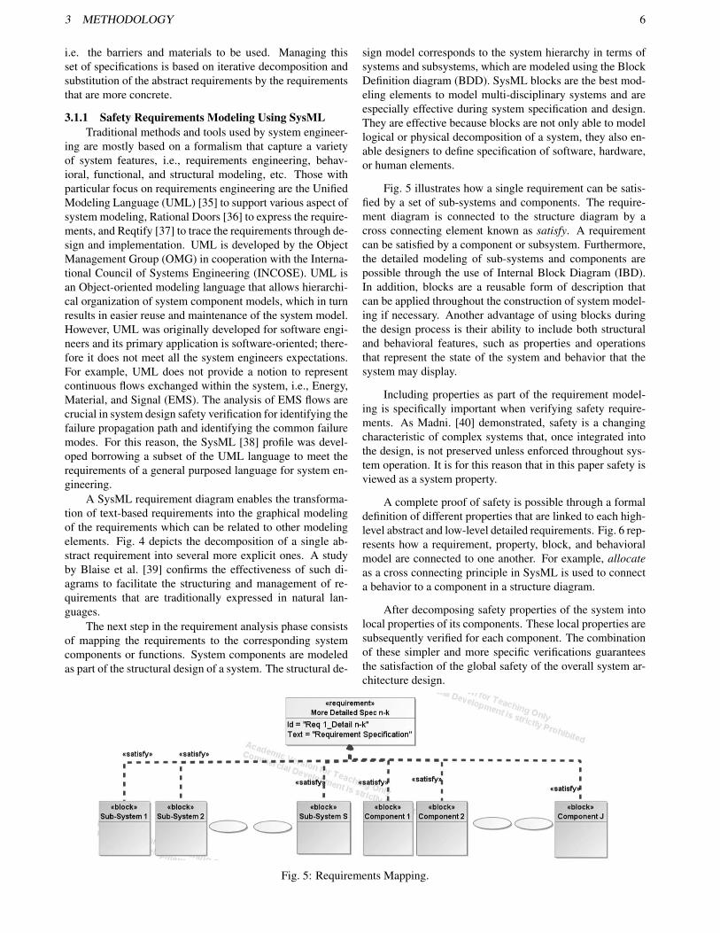
Fig. 13: Time Evolution of Faulty Components’ Population Size (Origin of Failure: (Left Picture: EMA Engine) and (RightPicture: Sensor)).

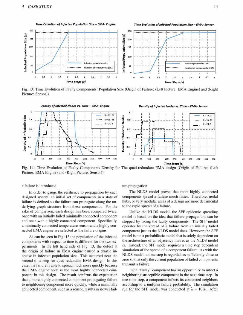
Fig. 14: Time Evolution of Faulty Components Density for The quad-redundant EMA design (Origin of Failure: (LeftPicture: EMA Engine) and (Right Picture: Sensor)).

a failure is introduced.

In order to gauge the resilience to propagation by eachdesigned system, an initial set of components in a state offailure is defined so the failure can propagate along the un-derlying graph structure from these components. For thesake of comparison, each design has been compared twice,once with an initially failed minimally connected componentand once with a highly connected component. Specifically,a minimally connected temperature sensor and a highly con-nected EMA engine are selected as the failure origins.

As can be seen in Fig. 13 the population of the infectedcomponents with respect to time is different for the two ex-periments. In the left hand side of Fig. 13, the defect atthe origin of failure in EMA engine caused a drastic in-crease in infected population size. This occurred near thesecond time step for quad-redundant EMA design. In thiscase, the failure is able to spread much more quickly becausethe EMA engine node is the most highly connected com-ponent in this design. The result confirms the expectationthat a more highly connected component propagating failureto neighboring component more quickly, while a minimallyconnected component, such as a sensor, results in slower fail-

ure propagation.The NLDS model proves that more highly connected

components spread a failure much faster. Therefore, nodalhubs, or very modular areas of a design are more detrimentalto the rapid spread of a failure.

Unlike the NLDS model, the SFF epidemic spreadingmodel is based on the idea that failure propagations can bestopped by fixing the faulty components. The SFF modeloperates by the spread of a failure from an initially failedcomponent just as the NLDS model does. However, the SFFmodel is not a probabilistic model that is solely dependent onthe architecture of an adjacency matrix as the NLDS modelis. Instead, the SFF model requires a time step dependentsimulation of the spread of a component failure. As with theNLDS model, a time step is regarded as sufficiently close tozero so that only the current population of failed componentstransmit a failure.

Each “faulty” component has an opportunity to infect aneighboring susceptible component in the next time step. Inone time step, a component infects its connected neighborsaccording to a uniform failure probability. The simulationrun for the SFF model was conducted at λ = 10%. After

4 CASE STUDY 15

a component has had an opportunity to infect its neighbors,the infected component would then be fixed in the conceptualdesign to resist the same failure according to the probabilityof failure removal µ = 10%. A repaired component is eitherconsidered faulty without the ability to transfer the failureto the neighboring components or is susceptible but resis-tant to the failures of its connected neighbors. Therefore, thecascading failure could be stopped with the provision thatenough faulty components become repaired in the design be-fore they are able to fully propagate the failure. That is, prop-agations can be halted if all transmission routes are blockedby repaired components.

The same designs were used with the epidemic spread-ing model as were used with the NLDS model. Additionally,the same initial failure conditions were used. A temperaturesensor was initially failed as a minimally connected compo-nent. An EMA engine node was then initially used to prop-agate the failure as a highly connected component. Fig. 14shows the epidemic spreading graphs.

In the SFF algorithm, the failure propagation is based onconnections, therefore the results must be reported in termsof faulty component density. As it is depicted in Fig. 14,each colored data set is representative of a set of componentswith the same degree e.g. red colored data set represents62 components in the system design with only three connec-tions. Therefore, each set of components has a failure den-sity ranging from 0 to 1; 0 representing that no componentsof that degree are infected and a 1 representing every compo-nent of that degree being infected. Fixed components are notconsidered faulty. Consequently, a plot of faulty componentdensity fluctuates intermittently between 0 and 1, howevereventually settles at 0 as all failed components are fixed inthe system design. In the legend of each graph, a k valueis given which is indicative of the degree of the componentsfollowed by the number of components within that data set.When a minimally connected component, such as a temper-ature sensor, is chosen as a failure origin, it is compared toan initially infected highly connected component, such as anEMA engine, the cascade spreads much slower, as expected.Three most representative sets in each figure is chosen anddrawn.

The left hand side of Fig. 14, illustrates the simulationresults for an initially failed, highly connected EMA en-gine. The plots present more immediate increases in infec-tion density, regardless of component degree when a highlyconnected component is failed initially. However, once theinitial infection has passed, and the failure density begins tosubside, the infection density is reduced. This is because astopped failure gets repaired probabilistically according to auniform rate.

However, it is possible to extend the LTS model of<Sa f eOpn> to constrain the number of failures in a waythat the system never reaches the catastrophic failure. For ex-ample, in the case of quad-redundant EMAs, the system cantolerate up to three failures without reaching the catastrophicfailure condition. This way, system designers can impose anew requirement of the form “if up to N number of EMAs failthen the catastrophic failure condition shall not occur.”. To

achieve this, the following generic (or parameterized) safetyproperty with the following constants and a range definitionsis used:

const N =4 \\ number of faulty EMAs 1

const M =4 \\ number of EMAsrange EMAs = 1..M \\ EMA identities

In order to prevent the system from reaching the catas-trophic event of <timeout>, it is essential to completethe mission and provide the required loads based onthe command signal. Therefore, the events of interestare the sent command signal, the jammed actuators, andthe completion of the mission. Consequently, as de-picted in the LTS model of Fig. 15 <Fault Tolerance>property contains {<commandLoad[1..4],d[1..4].jam, andmissionComplete>} actions. The property of Table 8, main-tains a count of faulty EMAs with the variable f . To modelthe fact that every command signal must be followed by a<missioncomplete>, the processes in line #3 and 8 are re-quired to constrain the number of faulty EMAs (f ) to a num-ber defined by the parameter of the property (N).

Table 8: FSP Model of Fault Tolerance Property

1 : property

2 : Fault Tolerance(N=4) = Jammed[0],

3 : Jammed[f : 0..M] =(when(f ≤ N)commandLoad[L] → Complete-Mission[f]

4 : |when (f>N) commandLoad[L]→ Jammed[f]

5 : |d[EMAs].jam→ Jammed[f+1]

6 : |missionComplete→ Jammed[f]),

7 : CompleteMission[f:0..M] = (missionComplete→ Jammed[f]

8 : |when (f<N ) d[EMAs].jam→ CompleteMission[f+1]

9 : |when (f==N) d[EMAs].jam→ Jammed[f+1]).

As can be seen in the compositional model of Table 9,the <Fault Tolerance> property is predefined with N = 2.Therefore, permitting only two out of four EMAs to fail dur-ing the system operation. Safety analysis using the LTS an-alyzer verifies that the safety property is satisfied. The com-posed LTS model of Table 9 consists of 242 states, howeverthe verification algorithm reduced the number of states to10733. The same result is obtained with three EMAs failing.

However, when the property is instantiated allowing four

Table 9: Compositional Model Of The System And SafetyProperty

1 : ‖Extend CommandUnit=(Fault Tolerance(2)‖CommandUnit)

2 : /shaft.reset/resetShaft.

3 : ‖Check Property =(Extend CommandUnit‖RedundantSystem).

1by default is set to 4 but it can be redefined during the instantiationprocess.

6 CONCLUSION AND FUTURE WORK 16

0 1 2 3 4-1 5 6 7

d[1..4].jam

missionComplete

d[1..4].jam

missionComplete

d[1..4].jam

missionComplete

d[1..4].jam

commandLoad[1..4],missionComplete commandLoad[1..4],

missionComplete

commandLoad[1..4]

commandLoad[1..4]

commandLoad[1..4]

d[1..4].jamd[1..4].jam

d[1..4].jam

missionCompleted[1..4].jam

commandLoad[1..4]

missionComplete

commandLoad[1..4] missionComplete

commandLoad[1..4]

Fig. 15: LTS Model Of The Fault Tolerance Property.

EMAs to fail, the safety analysis verifies that the property isviolated and a failure propagation path similar to the one inTable 7 is produced. Therefore, the generic safety propertymodeled in Table 8 verifies that the system never reaches thefailure condition of total loss if and only if N ≤ M-1 whereN is the number of faulty EMAs and M is the total numberof EMAs.

5 DiscussionFrom the result of case study: the characterization of the

system architecture by its subsystems and components, theFSP annotation of the failure behavior of each of them, andthe system level safety analysis based on components’ inter-action lead to achieving a manageable verification procedure.As compositional reasoning approach significantly reducesthe number of states to be explored, exhaustive checking ofthe entire state space is made feasible. This is especially im-portant where the exhaustive simulation is too expensive andnon-exhaustive simulation can miss the critical safety viola-tion.

A couple of telling conclusions can be drawn from theresult of the case study. Firstly, the NLDS models showedthat connectivity plays a major role in how fast an epidemicspreads. A few components with a higher degree increase thespeed of infection throughout a system. The NLDS modeladequately identified those design components that are criti-cal to a system and whose failure would cause shutdown ofthe whole system, as can be seen by the differences in fail-ure origins. Conversely, the SFF model can be used to com-pare different conceptual design architectures for resilienceto propagation. This can be done by analyzing how a failure

propagates through a system and then fixing failed compo-nents to inhibit the propagation of the failure. Both modelsprovide insight into design architectures that can be more re-silient to failures.

Furthermore, this type of safety analysis are very helpfulduring the early stages of the design because they providethe required information to implement the appropriate levelof component redundancies. It is important to note that, eventhough the application of component redundancy improvessystem reliability, it also adds cost, weight, size, and higherpower consumption.

6 Conclusion and Future WorkIn this research, resilience is addressed from different

viewpoints and a framework is presented that jointly enablesthe design of resilient systems. Resilience design is consid-ered an ability to design a system that is able to predict andprevent failure through exhaustive verification and by usingautomated assume-guarantee reasoning technique. Secondly,resilience design is characterized as part of the physical in-frastructure of the design that is robust and has the abilityto survive disruptions. Lastly, through the resilience designapproach, system is designed to recover from disruptions byattempting to return to the pre-disruption state.

In addition, this research clarifies the difference betweensafety and resilience. Safety is characterized as an emergingbehavior of the system that results from interactions amongsystem components and subsystems, including software andhumans. This is where designing a resilient system playsa crucial role in developing a proactive design practice forexploiting insights on faults in complex systems. In this con-text, system failure is viewed as an inability of the system to

REFERENCES 17

adapt and recover from disruptions, rather than components’and subsystems’ breakdown or malfunction.

Importantly, this work presented a framework for assess-ing and improving the resilience of complex systems duringthe early design process. The framework comprises failureprediction and prevention techniques, analysis of the effectof design topology on the propagation of failures, and pro-vides methodologies for system recovery from disruptions.The reason for these layers of analysis is to provide the sys-tem designers a set of tools to support them to integrate safetyand resilience where needed.

This work presented a compositional verification ap-proach and its novel application in the area of system de-sign and verification through pre-verification of system com-ponents and compositional reasoning. The aim of composi-tional reasoning is to improve scalability of the design verifi-cation problem by decomposing the original verification taskinto subproblems. Also, two propagation models, a Non-Linear Dynamical System (NLDS) model and an epidemicspreading model, are studied to be used during the early de-sign of complex systems. From the two models, equationsare provided to model the propagation characteristics of fail-ures in complex engineered systems. The NLDS propaga-tion model provides an indication for the length of time tofull propagation according to a graph layout. The SFF epi-demic spreading model provides an indication of the extentof a cascade according to a graph layout.

Future work will extend the existing verification tech-nique to include systems that exhibit probabilistic behavior.The approach will be based on the multi-objective proba-bilistic model checking. Properties of these models are for-mally defined as probabilistic safety properties. Further-more, the behavioral modeling and the automata learning al-gorithms require modification to support non-deterministicsystems. It is also necessary to explore symbolic implemen-tation of the algorithms for increased scalability.

In addition this work presented a new technique for anal-ysis of failure behavior for systems, based on design archi-tecture. The proposed technique enables system designersto assess failure behavior from the analysis of componentsof the system, however, these algorithms have to expandedso they can assess the probability of system-level failuresbased on failures of components. This approach should beconnected to a probabilistic model checker, which will allowverification of the failure models.

References[1] Chase, K. W., and Parkinson, A. R., 1991. “A survey of

research in the application of tolerance analysis to thedesign of mechanical assemblies”. Research in Engi-neering design, 3(1), pp. 23–37.

[2] Martin, M. V., and Ishii, K., 2002. “Design for variety:developing standardized and modularized product plat-form architectures”. Research in Engineering Design,13(4), pp. 213–235.

[3] Ameri, F., Summers, J. D., Mocko, G. M., and Porter,M., 2008. “Engineering design complexity: an inves-

tigation of methods and measures”. Research in Engi-neering Design, 19(2-3), pp. 161–179.

[4] Paries, J., 2006. “Complexity, emergence, resilience”.Hollnagel, E., Woods, dd, Leveson, N.(editors). Re-silience Engineering. Concepts and Precepts. Ashgate.

[5] Bedau, M. A., 2002. “Downward causation and theautonomy of weak emergence”. Principia, 6(1), pp. 5–50.

[6] Chalmers, D. J., 2002. “Varieties of emergence”. De-partment of Philosophy, University of Arizona, USA,Tech. rep./preprint.

[7] Seager, W., 2012. “Emergence and supervenience”. InNatural Fabrications. Springer, pp. 121–154.

[8] Pavard, B., Dugdale, J., Saoud, N. B.-B., Darcy, S.,and Salembier, P., 2006. “Design of robust socio-technical systems”. Resilience engineering, Juan lesPins, France.

[9] Leveson, N. G., 2002. “System safety engineering:Back to the future”. Massachusetts Institute of Tech-nology.

[10] Leveson, N., 2004. “A new accident model for engi-neering safer systems”. Safety science, 42(4), pp. 237–270.

[11] Hollnagel, E., Woods, D. D., and Leveson, N., 2007.Resilience engineering: Concepts and precepts. Ash-gate Publishing, Ltd.

[12] Cepin, M., 2011. “Reliability block diagram”. InAssessment of Power System Reliability. Springer,pp. 119–123.

[13] Do, D., 1980. “Procedure for performing a failuremode, effects and criticality analysis”. Department ofDefense, Washington DC.

[14] Stone, R. B., Tumer, I. Y., and Van Wie, M., 2005. “TheFunction-Failure Design Method”. Journal of Me-chanical Design(Transactions of the ASME), 127(3),pp. 397–407.

[15] Tumer, I. Y., Stone, R. B., and Bell, D. G., 2003.“Requirements for a Failure Mode Taxonomy for Usein Conceptual Design”. In Proceedings of the In-ternational Conference on Engineering Design, ICED,Vol. 3, Paper 1612, Stockholm,, Sweden.

[16] Krus, D., and Lough, K. G., 2007. “Applying Function-Based Failure Propagation in Conceptual Design”.ASME.

[17] Lough, K. G., Stone, R. B., and Tumer, I., 2006. “TheRisk in Early Design (RED) Method: Likelihood andConsequence Formulations”. In 2006 ASME Interna-tional Design Engineering Technical Conferences andComputers and Information In Engineering Confer-ence, DETC2006, September 10, 2006-September 13.

[18] Devendorf, E., and Lewis, K., 2008. “Planning on mis-takes: An approach to incorporate error checking intothe design process”. In ASME 2008 International De-sign Engineering Technical Conferences and Comput-ers and Information in Engineering Conference, Amer-ican Society of Mechanical Engineers, pp. 273–284.

[19] Kurtoglu, T., Tumer, I. Y., and Jensen, D. C., 2010. “AFunctional Failure Reasoning Methodology for Evalu-

REFERENCES 18

ation of Conceptual System Architectures”. Researchin Engineering Design, 21(4), pp. 209–234.

[20] Lee, W.-S., Grosh, D., Tillman, F. A., and Lie, C. H.,1985. “Fault Tree Analysis, Methods, and Applica-tions? A Review”. Reliability, IEEE Transactions on,34(3), pp. 194–203.

[21] Ericson, C. A., 2005. “Event tree analysis”. HazardAnalysis Techniques for System Safety, pp. 223–234.

[22] Greenfield, M. A., 2001. “Nasa’s use of quantitativerisk assessment for safety upgrades”. Space safety, res-cue and quality 1999-2000, pp. 153–159.

[23] Stamatelatos, M., Dezfuli, H., Apostolakis, G., Ever-line, C., Guarro, S., Mathias, D., Mosleh, A., Paulos,T., Riha, D., Smith, C., et al., 2011. “Probabilisticrisk assessment procedures guide for nasa managersand practitioners”.

[24] Venkatasubramanian, V., Zhao, J., and Viswanathan, S.,2000. “Intelligent systems for hazop analysis of com-plex process plants”. Computers & Chemical Engineer-ing, 24(9), pp. 2291–2302.

[25] Hollnagel, E., 2004. Barriers and accident prevention.Ashgate Publishing, Ltd.

[26] Johnson, C. W., and Holloway, C. M., 2003. “The esa/-nasa soho mission interruption: Using the stamp acci-dent analysis technique for a software related mishap”.Software: Practice and Experience, 33(12), pp. 1177–1198.

[27] Berezin, S., Campos, S., and Clarke, E. M., 1998. Com-positional reasoning in model checking. Springer.

[28] Alur, R., Madhusudan, P., and Nam, W., 2005. “Sym-bolic Compositional Verification By Learning Assump-tions”. In Computer Aided Verification, Springer,pp. 548–562.

[29] Cobleigh, J. M., Giannakopoulou, D., and Pasareanu,C. S., 2003. “Learning Assumptions For CompositionalVerification”. In Tools and Algorithms for the Con-struction and Analysis of Systems. Springer, pp. 331–346.

[30] Giannakopoulou, D., Pasareanu, C. S., and Barringer,H., 2005. “Component Verification With Automati-cally Generated Assumptions”. Automated SoftwareEngineering, 12(3), pp. 297–320.

[31] Nam, W., and Alur, R., 2006. “Learning-based Sym-bolic Assume-guarantee Reasoning With Automaticdecomposition”. In Automated Technology for Verifi-cation and Analysis. Springer, pp. 170–185.

[32] Chaki, S., Clarke, E., Sinha, N., and Thati, P., 2005.“Automated Assume-guarantee Reasoning For Simula-tion Conformance”. In Computer Aided Verification,Springer, pp. 534–547.

[33] Mehrpouyan, H., Giannakopoulou, D., Brat, G., Tumer,I. Y., and Hoyle, C., 2013. “Complex system designverification using assumption generation”. In ASME2013 International Design Engineering Technical Con-ferences and Computers and Information in Engineer-ing Conference, American Society of Mechanical En-gineers.

[34] Ullman, D. G., 2002. “Toward the ideal mechanical

engineering design support system”. Research in Engi-neering Design, 13(2), pp. 55–64.

[35] Booch, G., Rumbaugh, J., and Jacobson, I., 1999. Theunified modeling language user guide. Pearson Educa-tion India.

[36] Rational DOORS.[37] Geensoft, R. Effective solution for managing require-

ments traceability and impact analysis across hardwareand software projects lifecycle.

[38] Friedenthal, S., Moore, A., and Steiner, R., 2011. Apractical guide to SysML: the systems modeling lan-guage. Elsevier.

[39] Blaise, J.-C., Lhoste, P., and Ciccotelli, J., 2003. “For-malisation of normative knowledge for safe design”.Safety Science, 41(2), pp. 241–261.

[40] Madni, A., 2007. “Designing for resilience”. ISTI Lec-ture Notes on Advanced Topics in Systems Engineering.

[41] Henzinger, T., and Sifakis, J., 2006. “The EmbeddedSystems Design Challenge”. pp. 1–15.

[42] Pnueli, A., 1977. “The Temporal Logic of Programs”.In Foundations of Computer Science, 1977., 18th An-nual Symposium on, IEEE, pp. 46–57.

[43] Giannakopoulou, D., Pasareanu, C. S., and Barringer,H., 2002. “Assumption Generation for Software Com-ponent Verification”. In Automated Software Engineer-ing, 2002. Proceedings. ASE 2002. 17th IEEE Interna-tional Conference on, IEEE, pp. 3–12.

[44] Cobleigh, J., Giannakopoulou, D., and Pasareanu, C.,2003. “Learning Assumptions for Compositional Ver-ification”. Tools and Algorithms for the Constructionand Analysis of Systems, pp. 331–346.

[45] Cheung, S. C., and Kramer, J., 1999. “Checking SafetyProperties Using Compositional Reachability Analy-sis”. ACM Transactions on Software Engineering andMethodology (TOSEM), 8(1), pp. 49–78.

[46] Henzinger, T. A., Qadeer, S., and Rajamani, S. K.,1998. “You assume, we guarantee: Methodologyand case studies”. In Computer Aided Verification,Springer, pp. 440–451.

[47] Giannakopoulou, D., Pasareanu, C. S., and Cobleigh,J. M., 2004. “Assume-guarantee verification of sourcecode with design-level assumptions”. In Proceedingsof the 26th International Conference on Software Engi-neering, IEEE Computer Society, pp. 211–220.

[48] Rodrigues, R. W., 2000. “Formalising UML ActivityDiagrams Using Finite State Processes”. In Proc. ofthe 3rd Intl. Conf. on the Unified Modeling Language,York, UK, Citeseer.

[49] Mehrpouyan, H., Haley, B., Dong, A., Tumer, I. Y., andHoyle, C., 2013. “Resilient design of complex engi-neered systems”. In ASME 2013 International DesignEngineering Technical Conferences and Computersand Information in Engineering Conference, AmericanSociety of Mechanical Engineers, pp. V03AT03A048–V03AT03A048.

[50] Stone, R., Tumer, I., and Van Wie, M., 2005. “TheFunction-failure Design Method”. Journal of Mechan-ical Design, 127(3), pp. 397–407.

REFERENCES 19

[51] Michelena, N. F., and Papalambros, P. Y., 1997. “A hy-pergraph framework for optimal model-based decom-position of design problems”. Computational Opti-mization and Applications, 8(2), pp. 173–196.

[52] McCulley, C., and Bloebaum, C., 1996. “A genetic toolfor optimal design sequencing in complex engineeringsystems”. Structural Optimization, 12(2-3), pp. 186–201.

[53] Braha, D., and Reich, Y., 2003. “Topological structuresfor modeling engineering design processes”. Researchin Engineering Design, 14(4), pp. 185–199.

[54] Palmer, R. S., and Shapiro, V., 1993. “Chain models ofphysical behavior for engineering analysis and design”.Research in Engineering Design, 5(3-4), pp. 161–184.

[55] Harris, T. E., 1974. “Contact interactions on a lattice”.The Annals of Probability, pp. 969–988.

[56] Marro, J., and Dickman, R., 2005. NonequilibriumPhase Transitions in Lattice Models. Cambridge Uni-versity Press.

[57] Durrett, R., 1999. “Stochastic Spatial Models”. SiamReview, 41(4), pp. 677–718.

[58] Bodden, D. S., Clements, N. S., Schley, B., and Jen-ney, G., 2007. “Seeded failure testing and analysis ofan electro-mechanical actuator”. In Aerospace Confer-ence, 2007 IEEE, IEEE, pp. 1–8.

[59] Aten, M., Towers, G., Whitley, C., Wheeler, P., Clare,J., and Bradley, K., 2006. “Reliability comparisonof matrix and other converter topologies”. Aerospaceand Electronic Systems, IEEE Transactions on, 42(3),pp. 867–875.

[60] Raimondi, G., McFarlane, R., Bingham, C., Atallah,K., Howe, D., Mellor, P., Capewell, R., and Whitley,C., 1998. “Large electromechanical actuation systemsfor flight control surfaces”.

[61] Balaban, E., Saxena, A., Goebel, K., Byington, C.,Watson, M., Bharadwaj, S., Smith, M., and Amin,S., 2009. “Experimental Data Collection And Mod-eling For Nominal And Fault Conditions On Electro-mechanical Actuators”. In Annual Conference of thePrognostics and Health Management Society, pp. 1–15.