total factor productivity growth in east asia: a two ... · total factor productivity growth in...
TRANSCRIPT
European Journal of Economics, Finance and Administrative Sciences
ISSN 1450-2275 Issue 14 (2008)
© EuroJournals, Inc. 2008
http://www.eurojournals.com
Total Factor Productivity Growth in East Asia: A Two
Pronged Approach
Ammara Mahmood
Ph.D Scholar at School of Management, Yale University
Tel: +203-7816239
E-mail: [email protected]
Talat Afza
Professor and Dean, Faculty of Business Administration
COMSATS Institute of Information Technology
Lahore Campus
Tel: +92-321-4476024; Fax: +92-42-9203100
E-mail: [email protected], [email protected]
Abstract
This paper is an attempt at explaining the East Asian growth miracle. Employing the DEA
approach and the Malmquist productivity index the Total Factor Productivity of eight East
Asian countries have been calculated over the period 1980-2000. Comparison of the
sample countries reveals that the frontier was defined by Malaysian and Indonesia while
South Korea caught up with the frontier countries in later years. In the second stage the
paper analyzes the factors responsible for the surge in total factor productivity experienced
by the sample countries. Based on a panel regression with random effects of the countries
over the time period 1980-2000, for the sample as a whole, secondary education was the
only variable that had a positive impact on TFP growth and efficiency growth while it was
insignificant for technical change. On the contrary, trade openness and foreign direct
investment were seen to be inconsequent as determinants of TFP growth and its
components. This highlights the fact that internal technological improvements as opposed
to foreign capital and technologies were the main determinants of TFP growth and
improvements in efficiency. However, our indicator for internal R&D, the number of
scientific and technical journal articles, does not help in explaining the observed
phenomenon. Overall, the explanatory variables chosen in our model help explain
efficiency change but are inconsequent in explaining shifts in the production frontier.
Keywords: Total Factor Productivity, DEA Approach, Malquist Productivity Index, East
Asian Economies
1. Introduction After suffering a setback to its popularity in the early 1960s due to the failure of the ‘formula’ theories
to achieve substantive growth in the Third World (for example, Rostow, 1960; Lewis, 1954; and
Solow, 1956), interest in the field of long-term growth has resurfaced on economists’ research agenda
since the 1980s (see, for instance, Romer, 1986; and Lucas, 1988). One of factors responsible for this
change has been empirical evidence of convergence in per capita incomes and output across nations
94 European Journal of Economics, Finance and Administrative Sciences - Issue 14 (2008)
(Martin & Sunley, 1998). This encouraging finding has led to a surge in the re-orientation of growth
theory, with particular respect to treating as endogenous to the growth process those factors that the
traditional neoclassical growth model classifies as exogenous; in particular, human capital and
technological change.
The birth of endogenous theory, combined with observed evidence of cross-country
convergence in per capita incomes and output, has channeled much of the recent work in the field of
new growth empirics in the direction of regional growth patterns and testing for convergence. At the
same time, the spectacular growth of the East Asian economies over the past three decades has held
policy makers around the globe spellbound.
The first wave of growth in Japan was followed by a wave of growth in the four East Asian
“Tigers”; namely, Hong Kong, South Korea, Singapore and Taiwan. The next wave of growth was
witnessed in Indonesia, Malaysia, and Thailand. Since 1960, these eight economies together have
grown about twice as fast as the rest of East Asia and the industrial economies, about three times as
fast as Latin America and South Asia, and about five times as fast as sub-Saharan Africa (Day, Smith,
Thomas & Yeaman, 2005). The East Asian growth “Miracle”, as described by the World Bank (1993),
has led to the penning down of vast and diverse literature on the debate regarding the determinants of
growth (see, for instance, Young, 1995; Kim and Lau, 1994; World Bank, 1993; and Pack and Page,
1994).
However, few researchers have studied the impact of growth in total factor productivity (TFP)
as a potential factor influencing economic performance of the East Asian economies over the past few
decades. And yet we see that improvements in efficiency have been significant in determining the
growth trajectories of many developed economies (Zachariadis, 2004). Owing to this crucial nature of
productivity growth, numerous authors have made improvements in TFP the locus of their studies. For
instance, Fare, Grosskopf, Norris and Zhang (1994) have calculated TFP growth in seventeen OECD
countries. Savvides and Zachariadis (1994) delve into a detailed study of the determinants of TFP
growth, and their role in enhancing the overall productivity of OECD countries. Zachariadis (2004)
also analyses the role of research and development expenditure on productivity growth and overall
growth in output for a sample of OECD economies.
Due to their concentration on TFP growth, the above mentioned studies have provided valuable
insights into the dynamics of growth in OECD countries. In the case of East Asia, similar studies are
seriously lacking. 1 With an attempt to bridge this gap in literature, this paper studies total factor
productivity in five high-growth East Asian economies; China, Indonesia, Malaysia, South Korea and
Thailand 2 over the period 1980-2000, following a two-pronged approach, whereby we first calculate
the growth in TFP, and then proceed to analyze the factors responsible for this growth.
The paper proceeds as follows: section II provides an overview of the current literature on
productivity growth and convergence and the determinants of TFP growth. Section III will continue by
providing an in-depth explanation of the methodology used to calculate TFP growth, and then
explicates the model that evaluates the simultaneous contribution of various factors to growth in TFP.
Section IV goes on to describe the data, while section V discusses the results of the two stages. Finally,
section VI concludes the paper.
2. Literature Review 2.1. Productivity Growth and Convergence
Several issues related to productivity growth have gained attention in recent years. The main focus has
been on the productivity slowdown in the U.S and European countries during the 1960s and 1970s.
1 Young (1995) is perhaps one of the few researchers who have examined productivity growth in the East Asian region. But Young’s analysis
underscores the role played by factor accumulation in the Miracle, rather than growth in productivity. 2 These countries are part of the “Miracle” series of economies identified by the World Bank (1993). Further details regarding the selection criteria are
given in section III.

95 European Journal of Economics, Finance and Administrative Sciences - Issue 14 (2008)
Simultaneously, countries like Japan were seen to report high levels of productivity growth (Fare et al.,
1994). The increase in productivity of newly industrialized countries was attributed to the convergence
phenomenon of the neo-classical growth framework. According to Martin and Sunley (1998),
economists’ interest has largely focused on two measures of convergence: beta and sigma convergence. 3 There have been numerous attempts to measure the speed of cross-country beta-convergence (see, for
example, Baumol, 1986; Romer, 1986; Barro and Sala-i-Martin, 1992a, 1992b, 1995). The general
conclusion from these studies is that only when attention is restricted to the set of richer OECD
countries is there some support for absolute convergence4.
Similarly, Fare et al. (1994) criticize the studies conducted by De Long (1988) and Baumol
(1986), contending that the latter present a strong case for convergence primarily due to their
incorporation of partial productivity measures, namely labor productivity. By focusing on TFP growth
and breaking it up into technical and allocative components, Fare et al. (1994) make insightful
contributions to exiting literature on growth theory. Our study has also been largely inspired by the
framework employed by Fare et al. (1994).
2.2. Studies regarding determinants of TFP growth
Recent studies on TFP have also sought to analyze the determinants of growth in productivity.
Zachariadis (2004), in his study of ten OECD countries, regresses TFP growth on R & D intensity 5
using the Aghion and Howitt (1998) framework, according to which, internal R & D strongly
determines the level of productivity growth in an economy. These findings are also supported by Keller
(2002), who estimates that up to 80% of growth in productivity originates in domestic R & D. Jones
(1995) contends that the number of scientists engaged in R & D provides an adequate measure of the
level of domestic R & D in an economy.
However, domestic R & D alone does not provide an adequate estimate for growth in TFP.
Keller (2002) states that the remaining 20% of an economy’s productivity growth is brought about via
a channel of imports and foreign technology transfers. It is believed that foreign technologies can shift
a country’s domestic technology frontier outwards by introducing new inputs and production
techniques not previously available (Keller, 2002). A number of papers, including Coe and Helpman
(1995), Crespo, Martin and Velazquez (2002) and Griffith, Stephen and Van Reenen (2000), have
shown that foreign sources of technology have been an important source of productivity growth for
developed economies.
Savvides and Zachriadis (2005) state that less developed countries often carry out little R & D
of their own, and therefore, for these economies, technology diffusion across international borders
assumes a crucial role as a propellant of growth in TFP. However, despite the vital importance of
international technology diffusion as a channel of TFP growth in the context peculiar to low and
middle income countries, only a handful of empirical studies have been carried out, such as Coe and
Helpman (1995) and Mayer (2001).
3 Beta-convergence among a group of economies is said to exist if the beta value for the regression of the growth rate of regional relative per capita
income over a given period on the level of regional relative per capita income at the beginning of the period is negative (Martin & Sunley, 1998). A
negative value of beta reveals a tendency for per capita incomes to equalize across economies; therefore, beta measures the speed of convergence. A
group of economies is said to be characterized by sigma-convergence if the dispersion (variance) of their relative per capita income levels decreases
over time. 4 Absolute convergence refers to the long-term tendency for per capita GDP to equalize, or converge, across economies. The value of beta measures the
speed of the convergence process (Martin & Sunley, 1998). 5 R & D intensities for each economy are constructed as the fraction of output (gross domestic product) devoted to research and development
expenditures by an economy. See Zachariadis (2004) for further details on R & D intensity and its role in promoting growth in productivity.
96 European Journal of Economics, Finance and Administrative Sciences - Issue 14 (2008)
According to Wolff (1996), if an economy can increase its pace of technological progress by
means of capital imports that embody the latest technology, and by cross boarder transfer of
knowledge, its TFP growth will be higher. Zachariadis and Savvides (2005) argue that technology is
embodied in capital and intermediate goods, so that the direct import of these goods is a channel of
transmission of foreign technology, and hence eventual growth in TFP. This channel is consistent with
the models of Grossman and Helpman (1991), Francesco and Wilson (2004), and Eaton and Kortum
(2001). Moreover, according to Zachariadis (2004), openness can also have a positive impact on an
economy’s productivity growth through other channels, such as increased competition in the domestic
market.
Savvides and Zachriadis (2005) suggest that foreign direct investment (FDI) by multinational
corporations (MNCs) might be another channel for the international transmission of technology.
Besides the import of capital goods by the subsidiaries of MNCs, FDI frequently involves the
movement of employees and managerial talent across countries, as well as links between MNC
subsidiaries and local firms; all potential channels for the transfer of new technologies (Savvides and
Zachriadis, 2005). The issue of FDI spillovers has also been investigated by Borensztein, de Gregorio
and Lee (1998) and Xu (2000), to yield similar results.
A third approach to growth in productivity could be that of enrichment of human capital.
Papageorgiou (2002) underscores the great importance of human capital in the growth process. As
outlined by Nelson and Phelps (1966), and later built upon by Benhabib and Spiegel (1994), the
secondary enrollment ratio provides a valuable insight to the level of education within an economy,
which is crucial in the development of new technologies domestically and the effective absorption of
foreign technologies. Hence, gross secondary enrollment ratio (GSER) is an important determinant of
TFP growth. In their study of the manufacturing sectors of 32 economies over the period 1965 to 1992,
Savvides and Zachariadis (2005) have employed GSER as a variable in the determination of TFP.
3. Data Description Our dataset comprises the five economies of China, South Korea, Thailand, Malaysia and Indonesia
over the period 1980-2000. Japan has been excluded because it does not form part of the remarkable
East Asian “Miracle” that the region witnessed 1960 onwards, owing to its treading an individual,
separate trajectory altogether, in the growth process (World Bank, 1993). Moreover, a striking feature
of East Asian growth in recent years has been the increasing role of China’s economy in regional
economic activity and the significant shift in the pattern of East Asia’s trade (Day et al., 2005). China’s
economic rise is increasingly affecting East Asian growth dynamics, and we therefore feel it wise to
include China as part of our sample. Hong Kong has been left out on grounds of being a semi-
autonomous economy which is constitutionally within the realm of China, whereas Singapore and
Taiwan have not been included due to lack of availability of data.6
In order to calculate total factor productivity for the first part of our paper, we use data for
capital stock and labor as inputs in the Malmquist productivity index, and gross value added is taken to
be the output.
The primary data regarding capital, labor and gross value added have been obtained from the
Penn World Tables (PWT) Mark (6).7 PWT provides purchasing power parity and national income
accounts converted to international prices for 168 countries, for some or all of the years from 1950-
2000. All data is normalized to 1996 values8.
6 There was insufficient data regarding education and journal article publications for the observed time period for Taiwan and Singapore. Since these
variables are crucial to our study, we have excluded these economies from our study. 7 The European Union or the OECD provide more detailed purchasing power and real product estimates for their countries and the World Bank makes
current price estimates for most PWT countries at the GDP level. For further detail, refer to Heston, Summers and Aten (2002). 8 PWT 6.0 uses a substantially larger and more recent benchmark relative to PWT 5.6 that relates to 1996. The dataset consisted of 32 heading parties and
expenditure shares that were put together by the World Bank for 115 countries from various regional UN ICP comparisons. The underlying dataset
combined the comparisons of the EU, OECD, and other European and formerly Soviet countries for 1996, a total of 52 countries. The data then
combine International Comparison Program benchmark comparisons in different regions for either 1993 or 1996, with the former being brought
forward to 1996 (Heston, Summers & Aten, 2002).
97 European Journal of Economics, Finance and Administrative Sciences - Issue 14 (2008)
Owing to non-availability of reliable data on capital stock, investment was used as a proxy,
after employing the perpetual inventory method to discount for depreciation. This approach is in
conformity with that employed by Dimmerman (2003) and Dean (1964). Figures for investment were
obtained from the PWT. We use a ten percent rate of depreciation 9 to discount the annual investment
as given by the PWT.
Data for labor comprises the total working population of each of the five sample countries.
Similarly, GDP at constant prices was taken as a proxy for gross value added, in the absence of reliable
figures for the latter.
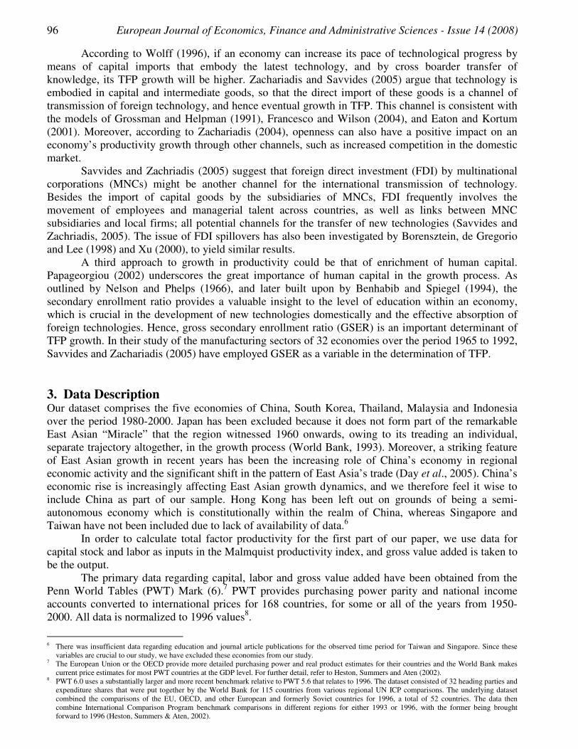
Table 1 shows the means and standard deviations for gross value added, capital and labor for
each country in the sample over the period 1980-2000.
Table 1: Summary Statistics: Gross Value Added, Labor and Capital 1980 – 2000
Country Gross Value Added Labor Capital
China 2252.1 0.658 1929.0
(1.417) (0.1046) (1363.)
Indonesia 483.92 0.078 380.02
(276.0) (0.016) (250.0)
Malaysia 118.62 0.007 134.70
(72.7) (0.0001) (9307)
South Korea 397.36 0.0019 631.07
(237.7) (0.0038) (426)
Thailand 245.49 0.0031 376.65
(143.4) (0.059) (251.2)
Average: 699.50 0.159 690.29 Note: The values for gross value added and capital are given in billions of constant 1996 US dollars, while the figures for labor represent billions of
people. Numbers in parentheses indicate standard deviations.
For the second part of our paper, we have employed a host of variables on which TFP has been
regressed. These variables are; gross secondary enrollment ratio (GSER), trade openness, number of
technical and scientific journal articles published, and gross foreign direct investment (GFDI).
According to the literature reviewed, these variables have been observed to have a significant impact
on growth in TFP.
The figures for GSER have been obtained from the database of World Development Report
(2005) and statistics of the UNESCO (2002). 10
These figures have been compiled for the period 1980-
2000. Data for Thailand and Malaysia were unavailable for a few years, and hence we used linear
interpolation/extrapolation techniques to fill in the gaps11
.
To gauge the extent to which an economy engages in international trade, we have obtained
figures for trade openness 12
from PWT version 6.1. PWT expresses import and export figures in
national currencies from the World Bank and United Nations data archives.
Publication of scientific and technical journal articles has been used to measure indigenous
research and development. These figures have been obtained from the World Development Report
(2005) for the period 1980-2000. FDI incorporates the import of capital goods by multinational
corporations (MNCs), and the transfer of managerial and technical skills resulting from the link
between parent companies and local subsidiaries of MNCs. The figures for FDI over the period 1980-
2000 have also been obtained from the World Development Report (2005).
9 For the manufacturing sectors of Pakistan and India, Burki, Khan and Bratsberg (1997) use rates of depreciation in the range 5 - 15 %. Since our study
focuses on all sectors of the economy, we feel that a ten percent rate of deprecation should be reasonable. 10 For further details, see the United Nations Educational, Social and Cultural Organization’s website www.unesco.org. 11 For Malaysia, data was missing for 1997, while for Thailand, data was missing for 1999.
12 Trade Openness = . CGDP
Exports Imports + See Heston, Summers and Aten (2002) for further details.
98 European Journal of Economics, Finance and Administrative Sciences - Issue 14 (2008)
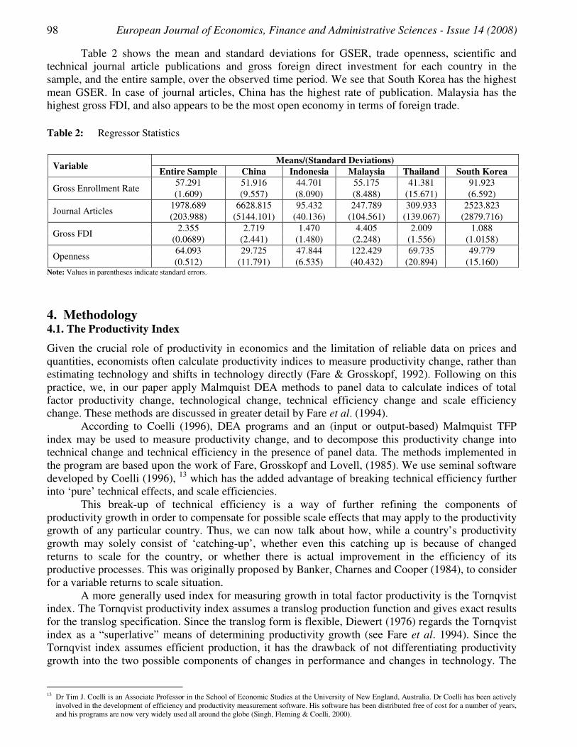
Table 2 shows the mean and standard deviations for GSER, trade openness, scientific and
technical journal article publications and gross foreign direct investment for each country in the
sample, and the entire sample, over the observed time period. We see that South Korea has the highest
mean GSER. In case of journal articles, China has the highest rate of publication. Malaysia has the
highest gross FDI, and also appears to be the most open economy in terms of foreign trade.
Table 2: Regressor Statistics
Variable Means/(Standard Deviations)
Entire Sample China Indonesia Malaysia Thailand South Korea
Gross Enrollment Rate 57.291 51.916 44.701 55.175 41.381 91.923
(1.609) (9.557) (8.090) (8.488) (15.671) (6.592)
Journal Articles 1978.689 6628.815 95.432 247.789 309.933 2523.823
(203.988) (5144.101) (40.136) (104.561) (139.067) (2879.716)
Gross FDI 2.355 2.719 1.470 4.405 2.009 1.088
(0.0689) (2.441) (1.480) (2.248) (1.556) (1.0158)
Openness 64.093 29.725 47.844 122.429 69.735 49.779
(0.512) (11.791) (6.535) (40.432) (20.894) (15.160) Note: Values in parentheses indicate standard errors.
4. Methodology 4.1. The Productivity Index
Given the crucial role of productivity in economics and the limitation of reliable data on prices and
quantities, economists often calculate productivity indices to measure productivity change, rather than
estimating technology and shifts in technology directly (Fare & Grosskopf, 1992). Following on this
practice, we, in our paper apply Malmquist DEA methods to panel data to calculate indices of total
factor productivity change, technological change, technical efficiency change and scale efficiency
change. These methods are discussed in greater detail by Fare et al. (1994).
According to Coelli (1996), DEA programs and an (input or output-based) Malmquist TFP
index may be used to measure productivity change, and to decompose this productivity change into
technical change and technical efficiency in the presence of panel data. The methods implemented in
the program are based upon the work of Fare, Grosskopf and Lovell, (1985). We use seminal software
developed by Coelli (1996), 13
which has the added advantage of breaking technical efficiency further
into ‘pure’ technical effects, and scale efficiencies.
This break-up of technical efficiency is a way of further refining the components of
productivity growth in order to compensate for possible scale effects that may apply to the productivity
growth of any particular country. Thus, we can now talk about how, while a country’s productivity
growth may solely consist of ‘catching-up’, whether even this catching up is because of changed
returns to scale for the country, or whether there is actual improvement in the efficiency of its
productive processes. This was originally proposed by Banker, Charnes and Cooper (1984), to consider
for a variable returns to scale situation.
A more generally used index for measuring growth in total factor productivity is the Tornqvist
index. The Tornqvist productivity index assumes a translog production function and gives exact results
for the translog specification. Since the translog form is flexible, Diewert (1976) regards the Tornqvist
index as a “superlative” means of determining productivity growth (see Fare et al. 1994). Since the
Tornqvist index assumes efficient production, it has the drawback of not differentiating productivity
growth into the two possible components of changes in performance and changes in technology. The
13 Dr Tim J. Coelli is an Associate Professor in the School of Economic Studies at the University of New England, Australia. Dr Coelli has been actively
involved in the development of efficiency and productivity measurement software. His software has been distributed free of cost for a number of years,
and his programs are now very widely used all around the globe (Singh, Fleming & Coelli, 2000).
99 European Journal of Economics, Finance and Administrative Sciences - Issue 14 (2008)
Malmquist index, on the contrary, does not require any assumptions regarding efficiency and
functional form, and is therefore able to distinguish between the factors causing changes in
productivity14
.
Given that we are analyzing a certain set of countries that have been specifically chosen for
their remarkable growth over the past two decades, the Malmquist index is a better way of deciding
how much of this growth is attributable to the ‘catching-up’ effect. Consequently, we calculate
productivity change as the geometric mean of two Malmquist productivity indices. This measure was
originally introduced by Caves, Christensen, Laurits and Diewert (1982a, b), and named after Sten
Malmquist, who had earlier proposed the idea of constructing quantity indices as ratios of distance
functions (Coelli, 1996). According to Fare et al. (1994), “distance functions are function
representations of multiple-output, multiple-input technology which require data only on output and
input quantities”. Fare et al. (1994) advocate the usage of a distance function to see whether the growth
in productivity is attributable to the above-mentioned catching up effect, described as improvements in
performance, or whether this growth is due to a shifting out of the technological frontier at a country’s
given set of inputs.
Since the Malmquist index gives measures of productivity changes over time, over every period
1,0, =tt ….T, the production technology tS is defined such that the inputs Nt Rx +∈ into output
Mt Ry +∈ . Hence, tttt xyxS :),{(= produces }ty . Although the Malmquist productivity index is
frequently used as an input-oriented index which determines the impact changes in inputs have over
productivity, it can also be defined as an output-based index. Fare and Grasskopf (1992) have set up
the input based Malmquist productivity index, while Fare et al. (1994) use the productivity based
Malmquist productivity index to determine TFP growth. Using an equivalent method developed by
Fare et al. (1989, 1992, 1994), we establish the output based productivity index. This index firstly
captures relative changes over time, using the ratio of distances from the productive frontier across
consecutive time periods. Pioneered by Shephard (1970), and later used by Fare (1988), the distance
function is defined as:
})/,(:inf{),(0
ttttttSyxyxD ∈= θθ
1}))/,(:(sup{ −∈= ttt Syx θθ
This function is defined as the reciprocal of the “maximum” proportional expansion of an
output given certain input combinations. When 1),(0 =tttyxD , it implies that ),( tt yx lies on the
boundary of the production frontier. In this case, the output is technically efficient. However,
1),(0 ≤tttyxD implies technical inefficiency. Similar results can be obtained for the input distance
function utilized by Deaton (1979), where the input distance function is defines as
}),/(:sup{),( tttttt
i SyxyxD ∈= λλ under constant returns to scale.
Under constant returns to scale production technology, maximum feasible output is only
achieved when average productivity ( xy / ) is maximized. The maximum, as will be shown in the next
section, is the benchmark country with the highest level of productivity. For the rest of the countries in
the sample, decreasing distances imply catching up to the maximum productive frontier, thus,
improving technical efficiency. This maximal level that is observed on the frontier is determined using
programming techniques that are explained later on.
To explain growth trends across periods of time the Malmquist productivity index gives
distance functions with respect to time. These are defined as follows:
})/,(:inf{),( 1111 tttttt
O SyxyxD ∈= ++++ θθ
),( 11 ++ ttt
O yxD measures the maximal proportional change in outputs to ensure that ( 11 , ++ tt yx ) is
feasible. At time period t, ( 11 , ++ tt yx ) is unattainable. 15
The maximal proportional change in output
14 For further details, see Fare et al. (1994).
100 European Journal of Economics, Finance and Administrative Sciences - Issue 14 (2008)
required to ensure the feasibility of ( tt yx , ) at t + 1 is denoted by ).,(1 ttt
O yxD+ Fare et al. (1994) define
the productivity index in period t as:
),(
),( !1
ttt
O
ttt
Ot
yxD
yxDM
++
=
Similarly, the Malmquist index for period t +1 is defined as follows:
),(
),(1
!111
ttt
O
ttt
Ot
yxD
yxDM
+
++++ =
Keeping in line with common practice and to avoid setting an arbitrary benchmark, we define
the Malmquist productivity index as the geometric mean of two Malmquist indices defined according
to the parameters in Caves et al. (1982a, b): 2/1
1
11111
11
),(
),(
),(
),(),,,(
=+
+++++++
ttt
o
ttt
o
ttt
o
ttt
otttt
OyxD
yxD
yxD
yxDyxyxM
This technique uses the ratios of two distance functions year on year in order to evaluate
productivity growth. This enables us to avoid setting any arbitrary benchmark, and we are able to use
two separate time-period distance functions to see how technological change can be shown using the
country’s distance functions16
.
Given the above specification, the level of the Malmquist index shows how productivity overall
is growing. An index value greater than 1 indicates growth in productivity, while values less than unity
show deterioration in the level of total factor productivity. Without looking at the efficiency and
technical change components, however, it is not possible for us to draw a comprehensive conclusion
about any changes in the level of productivity.
By rewriting the productivity index according to the method prescribed by Fare et al. (1989,
1992) we can distinguish between efficiency and technical change:17
=++ ),,,( 11 tttt
O yxyxM
2/1
1!11
11111
),(
),(
),(
),(
),(
),(
×
++++
+++++
ttt
o
ttt
o
ttt
o
ttt
o
ttt
o
ttt
o
yxD
yxD
yxD
yxD
yxD
yxD
Efficiency change × Technical change
Where: Efficiency change = ),(
),( 111
ttt
o
ttt
o
yxD
yxD+++
, Technical change =
2/1
1!11
11
),(
),(
),(
),(
++++
++
ttt
o
ttt
o
ttt
o
ttt
o
yxD
yxD
yxD
yxD
The value for efficiency change measures the overall change in relative efficiency, and is a
measure of the distance between observed production and the maximum possible production level
between the two time periods t and t + 1. The component for technical change, calculated as the
geometric mean of two ratios, measures the shift in production technology. This ratio represents the
relative change in the input technologies over the time period t and t + 1 (i.e. change in tx and 1+t
x ).
The availability of different indices for technical and efficiency change in the Malmquist index
make it even more appealing in the context of this paper. The sample countries all share the
characteristic of having exhibited exemplary growth over the past few decades (Day et al., 2005). It is,
therefore, quite insightful to make comparisons on the basis of technical change and efficiency change.
Thus, we will use the Malmquist index not only to evaluate net productivity growth, but also to see
15 Only when (
11 , ++ tt yx ) is obtained can it be concluded that technical change has taken place. 16 According to Fare et al. (1994), this form is typical to Fisher Ideal Indices. 17 Farrell (1957) developed a direct measure for calculating the distance functions of the Malmquist productivity index based on the relationship between
technical and efficiency change components. This approach has been adopted in this paper and is somewhat different from the manner in which Caves
et al. (1982a, b) employed the Malmquist index. For further detail, see Fare et al. (1994).
101 European Journal of Economics, Finance and Administrative Sciences - Issue 14 (2008)
whether this growth comes via the concept of improved utilization of existing resources (“catching-
up”) or through an outward shift in the production frontier. Although the Malmquist index can be used
for any type of returns to scale, for the purpose of analysis we define a constant returns to scale
production technology following Fare et al. (1994).
4.2. Determinants of TFP growth
After calculating TFP growth for the sample countries over the time period 1980-2000, it is the prime
objective of our study to examine the importance of several channels through which growth in TFP
occurs. Following up on previous studies, we incorporate three avenues of TFP growth simultaneously
in order to gauge the relative importance of alternative mechanisms: research and development (R &
D), international technology diffusion and human capital.
The number of scientific and technical journal publications by domestic scientists has been
employed as proxy for indigenous R & D as suggested by Nelson (1996). In addition to internal R&D
recent literature stresses the importance of foreign sources of technology as determinants of TFP
growth (see, for instance, Coe and Helpman, 1995; Crespo, Martin and Velazquez, 2002; Griffith,
Stephen and Van Reenen, 2000; Zachariadis, 2004; and Savvides and Zachriadis, 2005). Therefore, we
have incorporated both FDI and trade openness as explanatory variables in our model. Similarly,
secondary education has been seen to have a crucial role in explaining growth in TFP. Nelson and
Phelps (1966), Benhabib and Spiegel (1994) and Savvides and Zachriadis (2005) incorporate
secondary enrollment ratio in their studies of TFP. In light of this research practice, we have utilized
gross secondary enrollment ratio as a determinant of TFP growth in our study.
Hence, in the second stage of our paper, we regress values for growth in TFP measured using
the Malmquist index on gross secondary enrollment ratio, trade openness, the number of technical and
scientific journals published, and gross foreign direct investment. More specifically, we estimate the
following models: 20
1
4
20
1
3
20
1
2
20
1
1 itit
t
it
t
it
tt
itiit JOURNOPENFDIEDUCGTFP εααααββ ++++++= ∑∑∑∑====
(1)
......(20
1
4
20
1
3
20
1
2
20
1
1 itit
t
it
t
it
tt
itiit JOURNOPENFDIEDUCTECHCH εααααββ ++++++= ∑∑∑∑====
(2)
......(20
1
4
20
1
3
20
1
2
20
1
1 itit
t
it
t
it
tt
itiit JOURNOPENFDIEDUCEFFCH εααααββ ++++++= ∑∑∑∑====
(3)
We first look at the overall impact of the explanatory variables on TFP growth and then
proceed to look at the impact on the technical and efficiency change components of the Malmquist
productivity index. In these equations, iβ represents country-specific dummies which are included so
as to capture variation not attributable to the afore mentioned three avenues. itGTFP refers to growth in
TFP, itTECHCH is the growth in innovation over time, itEFFCH is the improvement in efficient
utilization of available inputs. itEDUC is the gross secondary school enrollment ratio, itFDI is the
gross foreign direct investment, itOPEN is the economy’s openness to foreign trade, and itJOURN is
the number of technical and scientific journal article publications taking place in the economy. The
intercept term β represents the estimated value of the dependant variable when all the independents
have a value of 0, while itε is the error term.

102 European Journal of Economics, Finance and Administrative Sciences - Issue 14 (2008)
5. Empirical Results 5.1. Results for TFP Growth
Given a single output (gross value added) and two inputs (capital and labor), we calculate technical
efficiency and total factor productivity for the five East Asian countries; China, Indonesia, Malaysia,
Thailand and South Korea, over the time period 1980-2000.
Technical efficiency in our context is defined with respect to the maximum attainable output
levels, while technology throughout the sample period is defined in terms of the output distance
function (see Fare et al., 1994). The best practice frontier constructed from the countries in the sample
represents the maximum level of output that can be obtained given the inputs. The frontier is based on
the assumption of constant returns to scale production technology. Given a single output and two
inputs, the best practice frontier is the equivalent of the production function of the most efficient
country in the sample.
Table 3 shows the results for technical efficiency for the sample countries over a five year
interval. 18
The distance from the frontier can be used to measure its levels of inefficiency.
Table 3: Technical Efficiency Across the Years
Technical Efficiency: Selected Years
(Constant Returns to Scale)
Year
Country 1981-85 1986-90 1991-95 1996-2000
China 1.151 1.099 1.070 1.282
Indonesia 1.000 1.000 1.000 1.000
Malaysia 1.000 1.001 1.000 1.000
Thailand 1.000 1.364 1.490 1.489
South Korea 1.179 1.000 1.000 1.000
Mean: 1.066 1.093 1.112 1.154
In the best practice frontier based on our sample of five East Asian countries, we see that over
the observed period, Indonesia and Malaysia defined the frontier and remained on the frontier
throughout. In 1990, South Korea caught up with the best practice frontier countries; as post-1990,
South Korea has maintained a technical efficiency figure of 1.00. Similarly, in 1995, China had a
figure of 1.00 for technical efficiency, and joined South Korea, Malaysia and Indonesia on the best
practice frontier. Thailand, on the contrary, has consistently been lying below the frontier, implying
that the country has been unable to attain technical efficiency in line with other countries in the region.
China also fell below the frontier in 2000. Overall, Indonesia and Malaysia have been the two most
efficient economies defining the frontier, followed by South Korea.
18 A value of 1 implies that the country lies on the best practice frontier, while a value greater than 1 suggests technical inefficiency, and that the country
lies below the frontier.
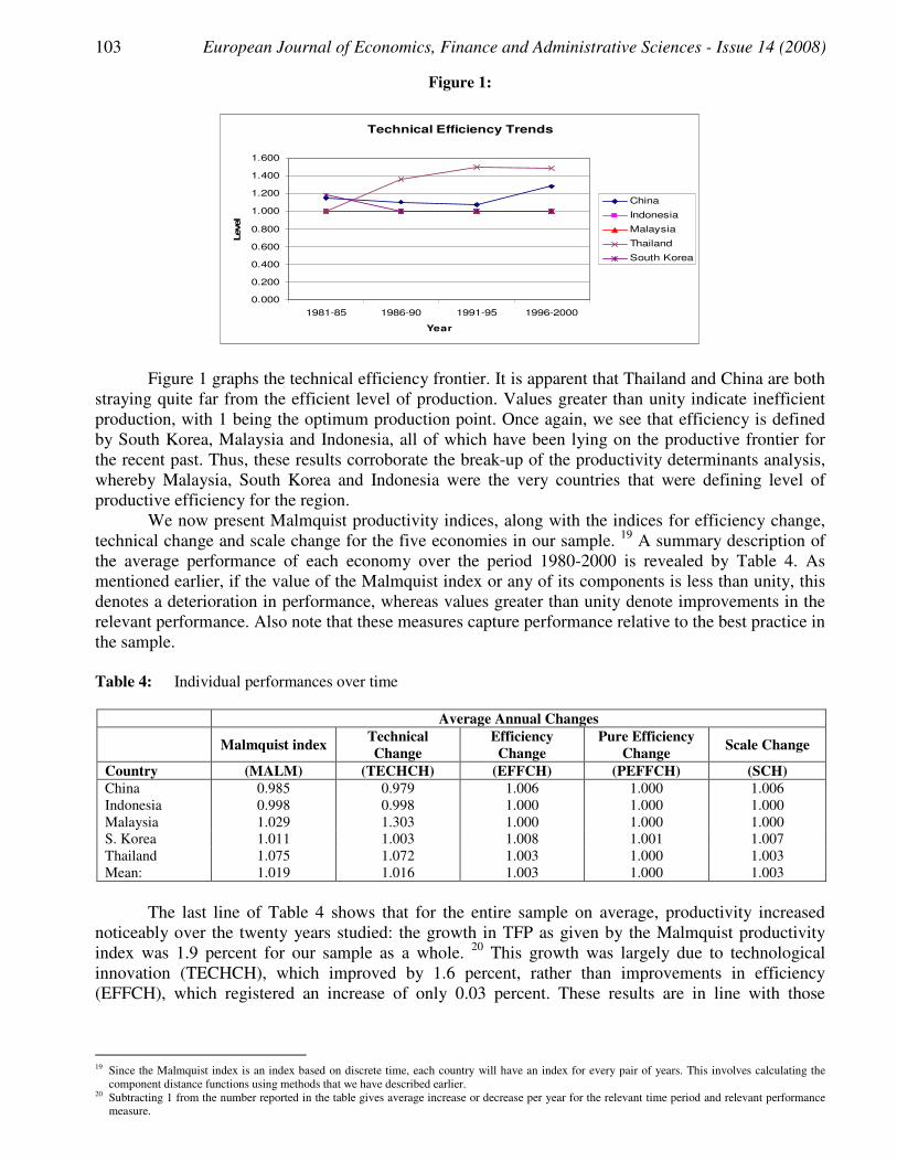
103 European Journal of Economics, Finance and Administrative Sciences - Issue 14 (2008)
Figure 1:
Technical Efficiency Trends
0.000
0.200
0.400
0.600
0.800
1.000
1.200
1.400
1.600
1981-85 1986-90 1991-95 1996-2000
Year
Level
China
Indonesia
Malaysia
Thailand
South Korea
Figure 1 graphs the technical efficiency frontier. It is apparent that Thailand and China are both
straying quite far from the efficient level of production. Values greater than unity indicate inefficient
production, with 1 being the optimum production point. Once again, we see that efficiency is defined
by South Korea, Malaysia and Indonesia, all of which have been lying on the productive frontier for
the recent past. Thus, these results corroborate the break-up of the productivity determinants analysis,
whereby Malaysia, South Korea and Indonesia were the very countries that were defining level of
productive efficiency for the region.
We now present Malmquist productivity indices, along with the indices for efficiency change,
technical change and scale change for the five economies in our sample. 19
A summary description of
the average performance of each economy over the period 1980-2000 is revealed by Table 4. As
mentioned earlier, if the value of the Malmquist index or any of its components is less than unity, this
denotes a deterioration in performance, whereas values greater than unity denote improvements in the
relevant performance. Also note that these measures capture performance relative to the best practice in
the sample.
Table 4: Individual performances over time
Average Annual Changes
Malmquist index Technical
Change
Efficiency
Change
Pure Efficiency
Change Scale Change
Country (MALM) (TECHCH) (EFFCH) (PEFFCH) (SCH)
China 0.985 0.979 1.006 1.000 1.006
Indonesia 0.998 0.998 1.000 1.000 1.000
Malaysia 1.029 1.303 1.000 1.000 1.000
S. Korea 1.011 1.003 1.008 1.001 1.007
Thailand 1.075 1.072 1.003 1.000 1.003
Mean: 1.019 1.016 1.003 1.000 1.003
The last line of Table 4 shows that for the entire sample on average, productivity increased
noticeably over the twenty years studied: the growth in TFP as given by the Malmquist productivity
index was 1.9 percent for our sample as a whole. 20
This growth was largely due to technological
innovation (TECHCH), which improved by 1.6 percent, rather than improvements in efficiency
(EFFCH), which registered an increase of only 0.03 percent. These results are in line with those
19 Since the Malmquist index is an index based on discrete time, each country will have an index for every pair of years. This involves calculating the
component distance functions using methods that we have described earlier. 20 Subtracting 1 from the number reported in the table gives average increase or decrease per year for the relevant time period and relevant performance
measure.

104 European Journal of Economics, Finance and Administrative Sciences - Issue 14 (2008)
obtained by Fare et al. (1994) for their sample of seventeen OECD countries for the time period 1979-
1988.
Moving on to the country-by-country results, we note that South Korea has the highest TFP
change in the sample, at 7.5% per annum on average, most of which can be attributed to improvements
in innovative ability. Indeed, South Korea’s rate of innovation was the highest in the five economies
studied. On the other hand, China exhibits a decrease in TFP of 1.5%, which is even lower than
Indonesia, where TFP fell by 0.2%. The other two countries in sample, i.e., Malaysia and Thailand
display positive, albeit lower, values for increase in TFP, of 2.9% and 1.1%, respectively.
Our small sample size, and the Korean economy’s considerably high value for technical change
(at 7.2%), allow us to conclude that South Korea, along with Malaysia, has played a significant role in
shifting the frontier outwards over time.
Figure 2:
Malmquist Index Trends
0.850
0.900
0.950
1.000
1.050
1.100
1.150
1981-85 1986-90 1991-95 1996-2000
Time
TF
P
China
Indonesia
Malaysia
Thailand
South Korea
For the purpose of meaningful and in-depth analysis, we have graphed the trends of total factor
productivity growth, efficiency change and technical change over five year intervals for all the
countries in our sample. Figure 2 illustrates that while overall productivity for the entire sample over
the observed period has increased, productivity for South Korea was the highest in 1980-85. Despite its
high economic growth in subsequent years, we see that growth in productivity has been continuously
declining over the observed period. However, despite the decline, TFP growth in South Korea has been
higher than all the other countries in the sample. China, on the other hand, has had the lowest level of
TFP growth. China’s TFP growth was at its minimum in the period 1986-90, after which productivity
showed a rising trend, and converged to the productivity levels of all other countries in the sample.
This stands to show that China’s focus on expanding the industrial and export base has simultaneously
resulted in productivity improvements. As for Malaysia, Indonesia and Thailand, their TFP growth has
remained in the vicinity of each other and followed similar trends, with Malaysia registering the
highest TFP growth. For these economies, average TFP growth peaked over the period 1986-90;
thereafter, it declined, and showed signs of recovery again in 1996-2000. Perhaps the beginning of the
financial crisis in these economies resulted in a slowdown in productivity growth in the early 1990s.
Since these graphs present average trends over five year intervals, it is not possible to pinpoint country
specific factors affecting TFP growth.

105 European Journal of Economics, Finance and Administrative Sciences - Issue 14 (2008)
Figure 3:
Efficiency Change Trends
0.900
0.920
0.940
0.960
0.980
1.000
1.020
1.040
1.060
1981-85 1986-90 1991-95 1996-2000
Time
Effic
iency C
hange
China
Indonesia
Malaysia
Thailand
South Korea
Figure 3 illustrates efficiency change over the five year intervals for the sample economies.
Through out the sample period we see that Indonesia and Malaysia maintained an efficiency index of 1
and did not register any improvements in efficiency. Since these countries already defined the
efficiency frontier we see no catching up for these two countries. After 1990 we see that South Korea
also joined these two efficient economies while Thailand shows a u-shaped pattern of efficiency
growth over the observed period. China is perhaps the most interesting economy as China’s efficiency
change pattern exhibited a zigzag shape over the observed time period; overall China has been unable
to catch up with the best practice countries.
Lastly, figure 4 shows the technical change component of the productivity index. It is
interesting to note that technical change in all five economies follow similar patterns as TFP growth as
a whole. This strengthens our earlier claim that TFP growth has been caused primarily due to technical
change that is innovation rather than improvements in efficiency. Perhaps the only difference that has
emerged is the fact that technical change rose steeply relative to TFP growth for Indonesia and China
in the period 1996-2000.
Figure 4:
Technical Change Trends
0.850
0.900
0.950
1.000
1.050
1.100
1981-85 1986-90 1991-95 1996-2000
Time
Technic
al C
hange
China
Indonesia
Malaysia
Thailand
South Korea
5.2. Results of Panel and OLS Estimation
The results for OLS and panel regressions with fixed and random effects are given in Table 5 while
Table 6 illustrates the results of panel regression on technical change and efficiency change.

106 European Journal of Economics, Finance and Administrative Sciences - Issue 14 (2008)
Table 5: Parameter estimates and summary statistics Panel and OLS regression of explanatory variables on
total factor productivity
Parameter estimates
Variable Standard OLS Fixed Effects Random Effects
Intercept 0.0098 0.8958
(0.000272679)** (0.054835)**
Gross Enrollment Ratio 0.1217 0.1463 0.1537
(0.031715)** (0.039032)** (0.041737)**
Openness -0.0578 -0.6727 -0.0605
(0.033375)* (0.045088) (0.034712)*
Gross FDI 0.0028 -0.0100 -0.0066
(0.010174) (0.010823) (0.010055)
Scientific and technical journal articles -0.0003 0.0397 0.0291
(0.000225098) (0.022003)* (0.025965)
Continuous time dummy -0.0041 -0.0041
(0.00196753)** (0.00187043)** 2R 0.1912 0.3642 0.2037
F-test of fixed effects 5.3791
(0.0006)**
Wu-Hausman test statistic 1.6658
[0.4348]
Note: Values in parentheses show standard errors, while those in square brackets are p-values. A single-asterisk Indicates statistical significance at α =
0.10 and double-asterisk indicates statistical significance at the 0.05 level.
Table 6: Parameter estimates and summary statistics for panel regression of explanatory variable on technical
change and efficiency change
Variable Parameter estimates
TECHCH EFCH
Intercept 0.9451 0.9685
(0.059923)** (0.046458)**
Gross Enrollment Ratio 0.0466 0.0776
(0.045619) (0.034340)**
Openness 0.0002 -0.0606
(0.037930) (0.029529)**
Gross FDI 0.0069 -0.0114
(0.010987) (0.00856910)
Number of scientific and technical journals 0.0065 0.0286
(0.028371) '(0.022165)
Continuous time dummy -0.00257167 -0.0017
(0.00204354) (0.00161659) 2R 0.0714 0.0903
Note: Values in parentheses show standard errors, while those in square brackets are p-values. A single-asterisk indicates statistical significance at α =
0.10 and double-asterisk indicates statistical significance at the 0.05 level.
In order to analyze the determinants of TFP growth, we regressed total factor productivity
growth for the entire sample against GSER, GFDI, journal articles and openness. The results are shown
in Table 5. The first column shows the ordinary least square estimates for GSER, GFDI, journal
articles and openness, along with t-values at the 10 % and 5 % significance levels. The second column
shows the results after taking into account country specific effects through the inclusion of country
dummies. The next two columns show the results for fixed effect and random effect 21
parameter
21 According to Greene (1997), panel data may have group effects, time effects, or both. These effects are either fixed effect or random effect. A fixed
effect model assumes differences in intercepts across groups or time periods while taking coefficients to be constant, whereas a random effect model
explores differences in error variances.

107 European Journal of Economics, Finance and Administrative Sciences - Issue 14 (2008)
estimates respectively. The panel estimates of the impact of GSER, GFDI, journal articles and
openness on technical change and efficiency change are given in Table 6.
Table 5 reveals that the fixed effects estimates yield the highest value for R-squared. 22
It is
interesting to note that OLS estimates which included dummies and a continuous time trend also give
the same value for 2R23
.
However, the Wu-Hausman test24
favors usage of the random effects model over the fixed
effects model. A glance at the test-statistic and the p-value indicates that the random effects estimators
are consistent and efficient. 25
Based on these statistics, it can be established that the random effects
specification best suits the sample countries.
These results are in tandem with Greene (2005), who highlights the problems that a fixed
effects specification can create. Fixed effects models tend to deplete degrees of freedom, which may
lead to increased standard errors. Also, fixed effects eliminate cross-sectional variance in the
independent variables, which again increases standard errors (and might make some standard errors
infinite, as in the case of variables that do not vary temporally). Moreover, they can exacerbate
problems of measurement error if the reliability of time-series variation in the explanatory variables is
poor (Greene, 2005).
For the regression on technical change and efficiency change 2R is higher with efficiency change
as the dependent variable as compared to technical change as the dependent variable. This shows that the
explanatory variables chosen in the model are more significant for the determination of efficiency change
relative to technical change. Overall Table 6 highlights the fact that despite the importance of technical
change in determining TFP growth, the explanatory variables that we have chosen are not adequate
determinants of technical change. On the contrary the variables that explain TFP growth provide a better
explanation of efficiency change.
We now proceed to interpret the parameter estimates for each variable under the random
specification for TFP growth and for its two components technical change and efficiency change.
For TFP growth gross secondary enrollment ratio has a positive value which is significant at the
5% level of significance.26
This implies that the level of secondary education is an important factor in
improving production technologies. Zachariadis (2005) in his study of TFP growth in OECD countries
obtains a similar positive relation between secondary enrollment and TFP growth. This result is also in
line with empirical literature on human capital which stresses the importance of education as an
essential component in improving production techniques, and hence productivity, especially in middle
and low income countries. Rodriguez-Claire (1997), Eicher (1996) and Restuccia (1997), all develop
models highlighting the importance of human capital in the adoption of new technologies and as a
determinant of productivity growth.
In the case of our sample countries, education has been a high priority, and there is a general
trend of encouraging vocational training. This is especially true for South Korea, as pointed out by
Holliday (2000), that the Korean state established a “productivist” welfare system, whereby education
was particularly promoted as a means of enhancing productivity and growth. Similarly, Davis (2003)
shows that during the period 1990 to 2000, China revamped its educational infrastructure. This was a
great improvement over the education system that prevailed during the 1980s, as our results show that
over the same period, China registered significant productivity improvements. Similar policies were
undertaken by the other countries in the region. It is therefore not surprising to see that governments’
objective of improving education has been directly correlated with productivity growth. This clearly
22 The fixed effects model includes country dummies as it implicitly takes into account country differentials, and therefore exhibits the highest 2R
(Ghura & Goodwin, 2000)
23 2R = 3.462
24 The Hausman specification test compares the fixed versus random effects under the null hypothesis OH that the random effects estimator is consistent
and efficient, while the fixed effects estimator is consistent, but not efficient (Greene 1997). 25 The Hausman test-statistic = 1.6658, p-value = 0.4348 26 The p-value for GSER is 0.000, which shows that the coefficient of GSER is highly significant.

108 European Journal of Economics, Finance and Administrative Sciences - Issue 14 (2008)
shows that improved education in our sample countries was important in improving the quality of
workers and their ability to utilize resources efficiently. Secondary enrollment ratio has not registered a
significant impact on technical change as table 6 shows the value is insignificant at the 5% level of
significance. On the other hand secondary enrollment ratio has had a significant positive impact on
technical change for the sample countries over the entire period. This clearly shows that secondary
education is an important variable in improving efficiency but does not directly lead to greater
innovation. Education has not played an important role in shifting the production function of the
sample countries; on the contrary secondary education has assisted relatively inefficient countries to
catch-up with the benchmark countries.
Helpman (1991), Caselli and Wilson (2004) and Eaton and Kortum (2001) hypothesized that
the direct import of capital and intermediate goods is a channel of transmission of foreign technology,
and hence eventual growth in TFP. However, for our sample trade openness has a statistically
significant negative value, 27
implying that high levels of imports and exports negatively impact TFP
growth for the sample countries over the period under observation. FDI is also observed to have
negative impact on productivity growth. Openness also has a significant negative value for efficiency
change but is insignificant in explaining technical change. The coefficient of GFDI appears to be
statistically insignificant for TFP growth as a whole, technical change and efficiency cahnge. Although
the coefficient of openness is negative, it is quite low, as only 6% of the growth in TFP can be
attributed to openness.
Similarly, the negative coefficient for FDI only explains 0.6% of the growth in TFP. This
means that FDI and trade openness are not the main factors affecting TFP. This is in line with
Zachariadis’s (2005) observation that FDI and trade do not significantly impact TFP growth; instead,
they have a stronger relationship with total value-added. Perhaps as Mayer (2001) points out, for
certain middle-income countries, the basic conditions for proper utilization of imported machinery or
capital may not exist, thereby hindering efficient production, and hence negatively impacting TFP. FDI
is crucial for capital accumulation, but it does not guarantee improvement in productivity. The negative
impact of trade openness on efficiency change contradicts the generally held belief that growth in East
Asia was primarily export-led and that these countries, especially South Korea, prospered by opening
up to the world market. On the contrary, internally developed technology and production methods
coupled with local policy initiatives have been a more important determinant of productivity growth
relative to the role played by foreign technology transfers and competition in the international market.
Internal research and development, as measured by the proxy, the number of scientific and
technical journal articles published, has a positive coefficient. However, this coefficient appears to be
statistically insignificant. 28
The coefficient for the components of TFP growth: technical change and
efficiency change, also register no significant relation with the number of scientific and technical
journal articles. This invalidates the choice of the proxy for research and development, as scientific and
technical journal articles do not have any substantial affect on the method of production. On the
contrary, actual expenditure on research and development in the form of R&D intensities has been
observed to be a more suitable variable explaining TFP growth. Zachariadis (2004), using R & D
expenditure as a fraction of GDP for 10 OECD countries over 1971-1995, shows that R & D has
significantly impacted TFP growth. Due to the unavailability of data on R&D expenditure for our
sample countries, we employed journal articles as proxy; however, as the results demonstrate, this was
not an appropriate proxy.
As Table 5 shows, the coefficient of the time trend has a statistically significant negative value. 29
This shows that TFP growth has shown a negative trend over time, as growth has tapered down over
the period. The slowdown in TFP growth over time could be attributed to the financial crisis that most
of these countries went through during the 1990s. According to Cho and Rhee (n. d.), Thailand, South
27 The p-value for trade openness is 0.081 which is significant at the 10% level of significance. On the other hand the coefficient of GFDI has a p-value of
0.511 which is statistically insignificant. 28 The value for the coefficient of the number of scientific and technical journal articles is 0.029 and the p-value is 0.263. 29 The estimated value for the coefficient of time trend in -0.0041

109 European Journal of Economics, Finance and Administrative Sciences - Issue 14 (2008)
Korea and Indonesia were particularly badly hit. Also in the case of South Korea, the large chaebols
have been criticized for the mismanagement arising from large scale production over time. As for the
components of TFP growth no significant relation with time has been observed.
Conclusively, our results for the determinants of TFP growth substantiate the literature on
human capital theory, as secondary enrollment is the most important determinant of productivity
growth over time. Foreign transfers of technology through increased trade and capital imports have not
had a significant impact on TFP growth. Thus, TFP growth can be attributed to internal technological
developments due to the highly educated labor force; however, over time, TFP growth has slowed
down. Incase of the components of TFP growth we observe that accumulation of human capital and
foreign capital transfers and trade have a significant impact on efficiency change, however as far as
technical change is concerned none of the variables in our model have been adequate in explaining
shifts in the frontier. Thus, the determinant variables in the second stage of our model are satisfactory
in explaining catching up among the sample countries however, our model does not provide insight
into the factors responsible for innovation responsible fro shifting the production frontier outwards,
6. Conclusion In light of the high growth in the East Asian economies, combined with the observed evidence of
cross-country convergence in per capita incomes and output, much of the recent work in the field of
new growth empirics has been directed towards the study of regional growth patterns and testing for
convergence. Similarly, there has been growing focus on the role of productivity growth in influencing
overall growth patterns of developed economies. Given the lack of research on the dynamics of
productivity growth in East Asia, this paper used the Malmquist productivity index to first calculate
TFP growth for China, Indonesia, Malaysia, South Korea and Thailand over the period 1980-2000, and
then proceeded to analyze the determinants of TFP growth.
Given the assumption of constant returns to scale production technology, the Malmquist
productivity index was used to construct the best practice frontier and to separate the technical and
efficiency components of TFP growth. In the best practice frontier based on the sample of five East
Asian countries, it was seen that over the observed period, Indonesia and Malaysia defined the frontier,
and remained on the frontier throughout. In 1990, South Korea caught up with the best practice frontier
countries, while Thailand remained the most technically inefficient economy.
For the entire sample on average, productivity increased noticeably over the twenty years. This
growth was largely due to technological innovation, rather than improvements in efficiency.
Improvement in the efficient utilization of resources was slower compared to the technological
innovation, as indicated by the larger value of the technical change component of the Malmquist index.
Following on with our two-pronged approach, the second stage of our study analyzed the
determinants of TFP growth and its components, namely efficiency change and technical change.
Based on a panel regression with random effects of the countries over the time period 1980-2000, for
the sample as a whole, secondary education was the only variable that had a positive impact on TFP
growth and efficiency growth while it was insignificant for technical change. On the contrary, trade
openness and foreign direct investment were seen to be inconsequent as determinants of TFP growth
and its components. This highlights the fact that internal technological improvements as opposed to
foreign capital and technologies were the main determinants of TFP growth and improvements in
efficiency. However, our indicator for internal R&D, the number of scientific and technical journal
articles, does not help in explaining the observed phenomenon. Overall, the explanatory variables
chosen in our model help explain efficiency change but are inconsequent in explaining shifts in the
production frontier.
After studying TFP growth and its possible determinants for the case of East Asia, the question
arises of what we have learnt from this exercise. And most importantly, can we evaluate government
policy in any country’s case, or suggest more suitable policy for the State to implement? According to
Felipe (1997), the results of growth accounting exercises or estimation of productivity values do not

110 European Journal of Economics, Finance and Administrative Sciences - Issue 14 (2008)
allow us to make an appraisal of the industrial policy and government intervention in any country.
Performing a TFP growth exercise with the aim of decomposing overall economic growth is not the
same as explaining the ultimate causes of growth. Therefore, most explanations about the growth of
countries stemming from increased productivity advanced by literature are unwarranted (Felipe, 1997).
As observed in our sample TFP growth levels in the chosen countries have little relationship to the
overall GDP growth. Thus we need to emphasize that in the catch-up phase of development for low-
and medium-developed countries governments should have a GDP growth-oriented focus rather than
worrying about the level of TFP growth.
However, the importance of education as an important determinant of TFP growth and overall
GDP growth cannot be undermined. The results of our study highlight the importance of education in
the development of innovative production technologies. Therefore, it can be advocated that
governments should focus more on domestic policy, especially education rather than having an
outward oriented approach in their efforts to improve TFP. It is important to keep in mind that different
models are applicable only under different assumptions, before drawing any conclusion from the
results. This, however, does not imply that studies on TFP growth have yielded dismissible results so
far. Thus, our study is a preliminary attempt to study the important determinants of TFP growth
without a focus on policy proposals. In future, we would like to further study in the area of technology
transfer on the lines of Savvides and Zachariadis (2005) and research the interaction between human
and physical capital more intensively as suggested by Felipe (1997).

111 European Journal of Economics, Finance and Administrative Sciences - Issue 14 (2008)
References 1] Aghion, P., & Howitt, P. 1992. “A model of growth through creative destruction”,
Econometrica,60, pp. 323-351.
2] Banker, R.D., Charnes, A., & Cooper, W.W. 1984. “Some models for estimating technical and
scale inefficiencies in data envelopment analysis”, Management Sciences, 30, pp. 1078-1092,
3] Baumol, W. 1986. “Productivity growth, convergence and welfare: What the long-run data
show”, American Economic Review, 76, pp. 1072-1085.
4] Barro, R.J., & Sala-i-Martin, X. 1992a. “Convergence”, Journal of Political Economy, 100, pp.
223-251.
5] Barro, R.J., & Sala-i-Martin, X. 1992b. “Regional growth and migration: A Japan-US
Comparison”, Journal of the Japanese and International Economies, 6, pp. 312-346.
6] Barro, R.J., & Sala-i-Martin, X. 1995. “Economic growth”, New York: McGraw Hill.
7] Benhabib, J., & Spiegel, M.M. 1994. “The role of human capital in economic development:
Evidence from cross-country date”, Journal of Monetary Economics, 34, pp. 143-173.
8] Borensztein, E., de Gregorio, J., & Lee, J. 1998. “How does foreign direct investment affect
economic growth”, Journal of International Economics, 45, pp. 115-135.
9] Burki, A.A., Khan, M.A., & Bratsberg, B. 1997. “Parametric tests of allocative efficiency in the
manufacturing sectors of India and Pakistan”, Applied Economics, 29, pp. 11-22.
10] Caves, D.W., Christensen, L.R., Laurits, R., & Diewert, W.E. 1982a. “Multilateral comparisons
of output, input, and productivity using index numbers”, Economic Journal, 92, pp. 73-86.
11] Caves, D.W., Christensen, L.R., Laurits, R., & Diewert, W.E. 1982b. “The economic theory of
index numbers and the measurement of input, output, and productivity”, Econometrica, 50, pp.
1393-1414.
12] Coe, D.T., & Helpman, E. 1995. “International R & D spillovers”, European Economic Review,
39, pp. 859-887.
13] Coelli, T.J. 1996. “Measurement of total factor productivity and biases in technological change
in Western Australian agriculture”, Journal of Applied Econometrics, 11, pp. 77-91.
14] Crespo, J., Martin, C., & Velazquez, F.J. 2002. “International technology diffusion through
imports and its impact on economic growth”, Manuscript, European Economy Group Working
Paper series, 12.
15] Davis, D. 2003. “China joins the global economy – part two”, Retrieved 14 February, 2006
from http://yaleglobal.yale.edu/display.article?id=2242.
16] Day, G., Smith, M., Thomas, B., & Yeaman, L. 2005. “The changing pattern of East Asia’s
growth”, Retrieved February 21, 2006 from http://www.treasury.gov.au/documents.
17] Dean, G., and Irwin, J.O. 1964. “The stock of fixed capital in the United Kingdom in 1961”,
Journal of the Royal Statistical Society. Series A (General), 127, pp. 327-358.
18] Deaton, A. 1979. “The distance function and consumer behavior with applications to index
numbers and optimal taxation”, Review of Economic Studies, 46, pp. 391-405.
19] De Long, J.B. 1988. “Productivity growth, convergence and welfare: Comment”, American
Economic Review, 78, pp. 1138-1154.
20] Diewert, W.E. 1976. “Exact and superlative index numbers”, Journal of Econometrics, 4, pp.
115-145.
21] Dimmerman, A.J. 2003. “Foreign R & D capital stock as a channel for technology transfer:
Latin America and Southeast Asia”, Retrieved 24 April, 2006 from
http://www.gwu.edu/~econ/job_cand/dimmerman_JMP.pdf.
22] Eaton, J., & Kortum, S. 2001. “Trade in capital goods”, European Economic Review, 45, pp.
1195-1235.
23] Eicher, T.S. 1996. “Interaction between endogenous human capital and technological change”,
Review of Economic Studies, 63, pp. 127-144.
24] Fare, R. 1988. “Fundamentals of production theory”, Lecture Notes in Economics and
Mathematical Sciences. Heidelberg: Springer-Verlag.

112 European Journal of Economics, Finance and Administrative Sciences - Issue 14 (2008)
25] Fare, R., & Grosskopf, S. 1990. “Theory and calculation of productivity indexes: Revisited”,
Discussion Paper No. 90-8, Southern Illinois University
26] Fare, R., Grosskopf, S., Lindgren, B., & Roos, P. 1989. “Productivity development in Swedish
hospitals: A Malmquist output index approach”, Discussion paper No. 89-3, Southern Illinois
University.
27] Fare, R., Grosskopf, S., Lindgreen, B., & Roos, P. 1992. “Productivity changes in Swedish
pharmacies, 1980 – 1989: A nonparametric Malmquist approach”, Journal of Productivity
Analysis, 3, pp. 85-101.
28] Fare, R., Grosskopf, S., Lovell, C.A.K. 1985. “The measurement of efficiency of production”,
Boston: Kluwer.
29] Fare, R., Grosskopf, S., Norris, M., & Zhang, Z. 1994. “Productivity growth, technical
progress, and efficiency change in industrialized countries”, The American Economic Review,
84, pp. 66-83.
30] Farrell, M.J. 1957. “The measurement of productive efficiency”, Journal of the Royal
Statistical Society, 120, pp. 253-81.
31] Felipe, J. 1997. “Total factor productivity growth in East Asia: A critical survey”, Manila:
Asian Development Bank.
32] Francisco, C. & Wilson, D. 2004. “Importing technology”, Journal of Monetary Economics, 51,
pp. 1-32.
33] Greene, D.P. 2005. “Analysis of panel data”, Retrieved 22 April, 2006 from
http://research.yale.edu/vote/pl504/.
34] Greene, W.H. 1997. “Econometric analysis”, New Jersey: Prentice Hall.
35] Griffith, R., Stephen, R., & Van Reenen, John. 2000. “Mapping the two faces of R & D:
Productivity growth in a panel of OECD industries”, Manuscript, Centre for Economic Policy
Research No. 2547.
36] Grossman, G., & Helpman, E. 1991. “Innovation and growth in the global economy”,
Cambridge, MA: MIT Press.
37] Helpman, E. 1999. “R & D and productivity: The international connection. In A. Razin & E.
Sadka (Eds.)”, The economics of globalization: Policy perspectives from public economics,
New York: Cambridge University Press.
38] Heston, A., Summers, R., & Aten, B. 2002. “Penn World Table” Version 6.1. Pennsylvania:
Center for International Comparisons, University of Pennsylvania (CICUP).
39] Holliday, I. 2000. “Productivist welfare capitalism: Social policy in East Asia”, Political
Studies, 48, pp. 706-723.
40] Jones, C.I. 1995. “R & D-based models of economic growth”, The Journal of Political
Economy, 103, pp. 759-784.
41] Keller, W. 2002. “Trade and the transmission of technology”, Journal of Economic Growth, 7,
pp. 5-24.
42] Kim, J.I., & Lau, L. 1994. “The sources of economic growth of the East Asian newly
industrialized countries”, Journal of Japanese and International Economics, 8, pp. 235-271.
43] Lucas, R.E. 1988. “On the mechanics of economic development”, Journal of Monetary
Economics, 22, pp. 3-42.
44] Lewis, W.A. 1954. “Economic development with unlimited supplies of labor”, The Manchester
School, 22, pp. 139-191.
45] Martin, R., & Sunley, P. 1998. “Slow convergence? The new endogenous growth theory and
regional development”, Economic Geography, 74, pp. 201-227.
46] Mayer, J. 2001. “Technology diffusion, human capital and economic growth in developing
countries”, UNCTAD Discussion Paper No. 154.
47] Nelson, R. 1996. “The sources of economic growth”, Cambridge: Harvard University Press.
48] Nelson, R.R., & Phelps, E.S. 1966. “Investment in humans, technological diffusion, and
economic growth”, American Economic Review, 56, pp. 69-75.

113 European Journal of Economics, Finance and Administrative Sciences - Issue 14 (2008)
49] Pack, H., & Page, J.M. 1994. “Accumulation, exports and growth in the high performing Asian
economies”, Carnegie-Rochester Conference Series on Public Policy, 40, pp. 199-236.
50] Papageorgiou, C. 2002. “Technology adoption, human capital and growth theory”, Review of
Development Economics, 6, pp. 351-368.
51] Restuccia, D. 1997. “Technology adoption and schooling: Amplifier income effects of policies
across countries”, University of Minnesota Working Paper.
52] Rodriguez-Claire, A. 1996. “Multinationals, linkages and economic development”, American
Economic Review, 86, pp. 852-873.
53] Romer, P. 1986. “Increasing returns and long-run growth”, Journal of Political Economy, 94,
pp. 1002-1037.
54] Rostow, W.W. 1960. “Stages of economic growth: A non-Communist manifesto”, Cambridge:
Cambridge University Press.
55] Savvides, A., & Zachariadis, M. 2005. “International technology diffusion and the growth of
TFP in the manufacturing sector of developing economies”, Review of Development
Economics, 9, pp. 482-501.
56] Shephard, R.W. 1970. “Theory of cost and production functions”, Princeton: Princeton
University Press.
57] Singh, S., Fleming, E., & Coelli, T.J. 2000. “Efficiency and productivity analysis of
cooperative dairy plants in Haryana and Punjab states of India”, Retrieved 14 April, 2006 from
http://www.une.edu.au/economics/publications/gsare.
58] Solow, R.M. 1956. “A contribution to the theory of economic growth”, Quarterly Journal of
Economics, 70, pp. 65-94.
59] United Nations Educational, Scientific and Cultural Organization. 2002. “UNESCO Institute
for Statistics”, Retrieved 15 March, 2006 from http://www.uis.unesco.org/.
60] Wolff, E.N. 1996. “The productivity slowdown: The culprit at last?”, American Economic
Review, 86, pp. 1239-1252.
61] World Development Report. 2005. “World Development Report 2005: A better investment
climate for everyone”, Retrieved 24 April, 2006 from http://econ.worldbank.org.
62] World Bank. 1993. “The East Asian miracle: Economic growth and public policy”, New York:
Oxford University Press.
63] Xu, B. 2000. “Multinational enterprises, technology diffusion, and host country productivity
growth”, Journal of Development Economics, 62, pp. 477-493.
64] Young, A. 1995. “The tyranny of numbers: Confronting the statistical realities of the East
Asian growth experience”, Quarterly Journal of Economics, 110, pp. 641-680.
65] Zachariadis, M. 2004. “R & D induced growth in the OECD?”, Review of Development
Economics, 8, pp. 423-439.