tosio kato’s work on non-relativistic quantum … · tosio kato’s work on non-relativistic...
TRANSCRIPT

Bull. Math. Sci. (2018) 8:121–232https://doi.org/10.1007/s13373-018-0118-0
Tosio Kato’s work on non-relativistic quantummechanics: part 1
Barry Simon1
Received: 8 November 2017 / Revised: 18 January 2018 / Accepted: 29 January 2018 /Published online: 22 February 2018© The Author(s) 2018. This article is an open access publication
Abstract We review the work of Tosio Kato on the mathematics of non-relativisticquantummechanics and some of the research that was motivated by this. Topics in thisfirst part include analytic and asymptotic eigenvalue perturbation theory, Temple–Katoinequality, self-adjointness results, and quadratic forms including monotone conver-gence theorems.
Keywords Kato · Schrödinger operators · Quantum mechanics
Mathematics Subject Classification Primary 81Q10 · 81U05 · 47A55; Secondary35Q40 · 46N50 · 81Q15
Contents
1 Introduction . . . . . . . . . . . . . . . . . . . . . . . . . . . . . . . . . . . . . . . . . . . . . . .2 Eigenvalue perturbation theory, I: regular perturbations . . . . . . . . . . . . . . . . . . . . . . . . .3 Eigenvalue perturbation theory, II: asymptotic perturbation theory . . . . . . . . . . . . . . . . . . .4 Eigenvalue perturbation theory, III: spectral concentration . . . . . . . . . . . . . . . . . . . . . . .5 Eigenvalue perturbation theory, IV: pairs of projections . . . . . . . . . . . . . . . . . . . . . . . . .6 Eigenvalue perturbation theory, V: Temple–Kato inequalities . . . . . . . . . . . . . . . . . . . . . .
Communicated by Ari Laptev.
B. Simon: Research supported in part by NSF Grants DMS-1265592 and DMS-1665526 and in part byIsraeli BSF Grant No. 2014337.
B Barry [email protected]
1 Departments ofMathematics andPhysics,Mathematics 253-37,California Institute of Technology,Pasadena, CA 91125, USA
123

122 B. Simon
7 Self-adjointness, I: Kato’s theorem . . . . . . . . . . . . . . . . . . . . . . . . . . . . . . . . . . .8 Self-adjointness, II: the Kato–Ikebe paper . . . . . . . . . . . . . . . . . . . . . . . . . . . . . . . .9 Self-adjointness, III: Kato’s inequality . . . . . . . . . . . . . . . . . . . . . . . . . . . . . . . . . .10 Self-adjointness, IV: quadratic forms . . . . . . . . . . . . . . . . . . . . . . . . . . . . . . . . . .References . . . . . . . . . . . . . . . . . . . . . . . . . . . . . . . . . . . . . . . . . . . . . . . . . .
1 Introduction
Note: There are four pictures in this part and one picture in Part 2.In 2017, we are celebrating the 100th anniversary of the birth of Tosio Kato (August
25, 1917–October 2, 1999).While there can be arguments as towhich of his work is thedeepest or most beautiful, there is no question that themost significant is his discovery,published in 1951, of the self-adjointness of the quantum mechanical Hamiltonian foratoms and molecules [314]. This is the founding document and Kato is the foundingfather of what has come to be called the theory of Schrödinger operators. So it seemsappropriate to commemorate Kato with a comprehensive review of his work on non-relativistic quantum mechanics (NRQM) that includes the context and later impact ofthis work.
One might wonder why I date this field only from Kato’s 1951 paper. After all,quantum theory was invented in 1925–1926 as matrix mechanics in Göttingen (byHeisenberg, Born and Jordan) and as wave mechanics in Zürich (by Schrödinger)and within a few years, books appeared on the mathematical foundations of quan-tum mechanics by two of the greatest mathematicians of their generation: HermannWeyl [681] (not coincidentally, in Zürich; indeed the connection between Weyl andSchrödinger was more than professional—Weyl had a passionate love affair withSchrödinger’s wife) and John von Neumann [664] (von Neumann, whose thesis hadbeen in logic, went to Göttingen to work with Hilbert on that subject, but was sweptup in the local enthusiasm for quantum theory, in response to which, he developed thespectral theory of unbounded self-adjoint operators and his foundational work). Oneshould also mention the work of Bargmann andWigner (prior to Kato, summarized in[579] with references) on quantum dynamics. I think of this earlier work as first levelfoundations and the theory of Schrödinger operators as second level. Another way ofexplaining the distinction is that the Weyl–von Neumann work is an analog of settingup a formalism for classical mechanics like the Hamiltonian or Lagrangian while thetheory initiated by Kato is the analog of celestial mechanics—the application of thegeneral framework to concrete systems.
123

Tosio Kato’s work on non-relativistic quantum mechanics: part 1 123
When I began this project I decided to write about all of Kato’s major contributionsto the field in a larger context and this turned into a much larger article than I originallyplanned.As such, it is a reviewof a significant fractionof theworkof the last 65years onthemathematics ofNRQM.Two important areas only touched on or totallymissing areN-body systems and the largeN limit. Of course, Kato’s self-adjointnesswork includesN-body systems, and there are papers on bound states in Helium and on properties ofmany body eigenfunctions. As we’ll see, his theory of smooth perturbations applies togive a complete spectral analysis of certain N-body systems with only one scatteringchannel and is one tool in the study of general N -body systems. But there is muchmore to the N-body theory—for reviews, see [101,116,197,212,264]. Except for the1972 work of Lieb–Simon on Thomas Fermi almost all the large N limit work is after1980 when Kato mostly left the field; for recent reviews of different aspects of thissubfield, see [51,424,425,428,429,529,551].
While this review will cover a huge array of work, it is important to realize it is onlya fraction, albeit a substantial fraction, of Kato’s opus. I’d classify his work into fourbroad areas, NRQM, non-linear PDE’s, linear semigroup theory and miscellaneouscontributions to functional analysis. We will not give references to all this work. Thereader can get an (almost) complete bibliography from MathSciNet or, for papers upto 1987, the dedication of the special issue of JMAA on the occasion of Kato’s 70thbirthday [122] has a bibliography.
Around 1980, one can detect a clear shift in Kato’s interest. Before 1980, thebulk of his papers are on NRQM with a sprinkling in the other three areas whileafter 1980, the bulk are on nonlinear equations with a sprinkling in the other areasincludingNRQM.Kato’s nonlinearwork includes looking at the Euler, Navier–Stokes,KdV and nonlinear Schrödinger equations. He was a pioneer in existence results—wenote that his famous 1951 paper can be viewed as a result on existence of solutionsfor the time dependent linear Schrödinger equation! It is almost that when NRQMbecame too crowded with workers drawn by his work, he moved to a new area whichtook some time to become popular. Terry Tao said of this work: the Kato smoothing
123

124 B. Simon
effect for Schrödinger equations is fundamental to the modern theory of nonlinearSchrödinger equations, perhaps second only to the Strichartz estimates in impor-tance…Kato developed a beautiful abstract (functional analytic) theory for local wellposedness for evolution equations; it is not used directly too much these days becauseit often requires quite a bit more regularity than we would like, but I think it wasinfluential in inspiring more modern approaches to local existence based on moresophisticated function space estimates.
And here is what Carlos Kenig told me: T. Kato played a pioneering role in thestudy of nonlinear evolution equations. He not only developed an abstract frameworkfor their study, but also introduced the tools to study many fundamental nonlinearevolutions coming from mathematical physics. Some remarkable examples of this are:Kato’s introduction of the “local smoothing effect” in his pioneering study of theKorteweg–de Vries equation, which has played a key role in the development of thetheory of nonlinear dispersive equations.
Kato’s unified proof of the global well-posedness of the Euler and Navier–Stokesequations in 2d, which led to the development of the Beale–Kato–Majda blow-upcriterion for these equations. Kato’s works with Ponce on strong solutions of the Eulerand Navier–Stokes equations, which developed the tools for the systematic applicationof fractional derivatives in the study of evolutions, which now completely permeatesthe subject. These contributions and many others, have left an indelible and enduringimpact for the work of Kato on nonlinear evolutions.
The basic results on generators of semigroups on Banach spaces date back to theearly 1950s going under the name Feller–Miyadera–Phillips and Hille–Yosida theo-rems (with a later 1961 paper of Lumer–Phillips). A basic book with references to thiswork is Pazy [475]. This is a subject that Kato returned to often, especially in the 1960s.Pazy [475] lists 19papers byKatoon the subject. There is overlapwith theNRQMworkand the semigroup work. Perhaps the most important of these results are the Trotter–Kato theorems (discussed below briefly after Theorem 3.7) and the definition offractional powers for generators of (not necessarily self-adjoint) semigroups. There arealso connections between quantum statistical mechanics and contraction semigroupon operator algebras. To keep this reviewwithin bounds, we will not discuss this work.
The fourth area is a catchall for a variety of results that don’t fit into the otherbins. Among these results is an improvement of the celebrated Calderón–Vaillancourtbounds onpseudo-differential operators [346]. In [342],Kato proved the absolute valuefor operators is not Lipschitz continuous even restricted to the self-adjoint operatorsbut for any pair of bounded, even non-self-adjoint, operators one has that
‖|S| − |T |‖ ≤ 2
π‖S − T ‖
(2 + log
‖S‖ + ‖T ‖‖S − T ‖
)(1.1)
(I don’t think there is any significance to the fact that the constant is the same as in(10.31)).
The last of these miscellaneous things that we’ll discuss (but far from the last ofthe miscellaneous results) involves what has come to be called the Heinz–Loewnerinequality. In 1951, Heinz [225] proved for positive operators, A, B on aHilbert space,one has that A ≤ B ⇒ √
A ≤ √B. Heinz was a student of Rellich and Kato was
123

Tosio Kato’s work on non-relativistic quantum mechanics: part 1 125
paying attention to the work of Rellich’s group and a year later published a paper[319] with an elegant, simple proof and extended the result to A �→ As for 0 < s < 1replacing the square root. Neither of them knew at the time that Loewner [436] hadalready proven a much more general result in 1934! Despite the 17 year priority, themonotonicity of the square root is called variably, the Heinz inequality, the Heinz–Loewner inequality or even, sometimes, the Heinz–Kato inequality. Heinz and Katofound equivalent results to the monotonicity of the square root (one paper with lots ofadditional equivalent forms is [180]). In particular, the following equivalent form isalmost universally known as the Heinz–Kato inequality.
‖T ϕ‖ ≤ ‖Aϕ‖, ‖T ∗ψ‖ ≤ ‖Bψ‖ ⇒ |〈ψ, T ϕ〉| ≤ ‖Asϕ‖‖B1−sψ‖ (1.2)
Kato returned several times to this subject, most notably [333] finding a version ofthe Heinz–Loewner inequality (with an extra constant depending on s) for maximalaccretive operators on a Hilbert space.
Returning to the timing of Kato’s fundamental 1951 paper [314], I note that hewas 34 when it was published (it was submitted a few years earlier as we’ll discuss inSect. 7). Before it, his most important work was his thesis, awarded in 1951 and pub-lished in 1949–1951. One might be surprised at his age when this work was publishedbut not if one understands the impact of the war. Kato got his BS from the Universityof Tokyo in 1941, a year in which he published two (not mathematical) papers intheoretical physics. But during the war, he was evacuated to the countryside. We wereat a conference together one evening and Kato described rather harrowing experiencesin the camp he was assigned to, especially an evacuation of the camp down a steepwet hill. He contracted TB in the camp. In his acceptance for the Wiener Prize [1],Kato says that his work on essential self-adjointness and on perturbation theory wereessentially complete “by the end of the war.” Recently, several of Kato’s notebookwere discovered dated 1945 that contain most of results published in Kato [314,316]sometimes with different proofs from the later publications (these notes have recentlybeen edited for publication in [358]).
123
126 B. Simon
In 1946, Kato returned to the University of Tokyo as an Assistant (a position commonfor students progressing towards their degrees) in physics, was appointed AssistantProfessor of Physics in 1951 and full professor in 1958. I’ve sometimeswonderedwhathis colleagues in physics made of him. Hewas perhaps influenced by the distinguishedJapanese algebraic geometer, Kunihiko Kodaira (1915–1997) 2years his senior and a1954 Fields medalist. Kodaira got a BS in physics after his BA in mathematics andwas given a joint appointment in 1944, so there was clearly some sympathy towardspure mathematics in the physics department. In 1948, Kato and Kodaira wrote a 2page note [360] to a physics journal whose point was that every L2 wave function wasacceptable for quantummechanics, something about which there was confusion in thephysics literature.
Beginning in 1954, Kato started visiting the United States. This bland statementmasks some drama. In 1954, Kato was invited to visit Berkeley for a year, I presumearranged by F. Wolf. Of course, Kato needed a visa and it is likely it would have beendenied due to his history of TB. Fortunately, just at the time (and only for a periodof about a year), the scientific attaché at the US embassy in Tokyo was Otto Laporte(1902–1971) on leave from a professorship in Physics at the University of Michigan.Charles Dolph (1919–1994), a mathematician at Michigan, learned of the problemand contacted Laporte who intervened to get Kato a visa. Dolph once told me that hethought his most important contribution to American mathematics was his helping toallow Kato to come to the US. In 1987, in honor of Kato’s 70th birthday, there was aspecial issue of the Journal of Mathematical Analysis and Applications and the issuewas jointly dedicated [122] to Laporte (he passed away in 1971) and Kato and editedby Dolph and Kato’s student Jim Howland.
During the mid 1950s, Kato spent close to 3years visiting US institutions, mainlyBerkeley, but also the Courant Institute, American University, National Bureau ofStandards and Caltech. In 1962, he accepted a professorship in Mathematics fromBerkeley where he spent the rest of his career and remained after his retirement.One should not underestimate the courage it takes for a 45year old to move to avery different culture because of a scientific opportunity. That said, I’m told thatwhen he retired and some of his students urged him to live in Japan, he said heliked the weather in Northern California too much to consider it. The reader canconsult the Mathematics Genealogy Project (http://www.genealogy.ams.org/id.php?id=32842) for a list of Kato’s students (24 listed there, 3 from Tokyo and 21 fromBerkeley; the best known are Ikebe and Kuroda from Tokyo and Balslev and Howlandfrom Berkeley) and [98] for a memorial article with lots of reminisces of Kato.
One can get a feel forKato’s impact by considering the number of theorems, theoriesand inequalities with his name on them. Here are some: Kato’s theorem (which usuallyrefers to his result on self-adjointness of atomic Hamiltonians), the Kato–Rellich the-orem (which Rellich had first), the Kato–Rosenblum theorem and the Kato–Birmantheory (where Kato had the most significant results although, as we’ll see, Rosenblumshould get more credit than he does), the Kato projection lemma and Kato dynamics(used in the adiabatic theorem), the Putnam–Kato theorem, the Trotter–Kato theorem(which is used for three results; see Sect. 3), the Kato cusp condition (see Sect. 19 inPart 2), Kato smoothness theory, the Kato class of potentials and Kato–Kuroda eigen-function expansions. To me Kato’s inequality refers to the self-adjointness technique
123

Tosio Kato’s work on non-relativistic quantum mechanics: part 1 127
discussed in Sect. 9, but the term has also been used for the Hardy like inequality withbest constant for r−1 in three dimensions (which we discuss in Sect. 10), for a resulton hyponormal operators that follows from Kato smoothness theory (the book [441]has a section called “Kato’s inequality” on it) and for the above mentioned variant ofthe Heinz–Loewner inequality for maximal accretive operators. There are also Heinz–Kato, Ponce–Kato and Kato–Temple inequalities. In [550], Erhard Seiler and I provedthat if f, g ∈ L p(Rν), p ≥ 2, then f (X)g(−i∇) is in the trace ideal Ip. At the time,Kato and I had correspondence about the issue and about some results for p < 2. In[496], Reed and I mentioned that Kato had this result independently. Although Katonever published anything on the subject, in recent times, it has come to be called theKato–Seiler–Simon inequality.
Of course, when discussing the impact of Kato’s work, one must emphasize theimportance of his book Perturbation Theory for Linear Operators [345] which hasbeen a bible for several generations of mathematicians. One of its virtues is its compre-hensive nature. Percy Deift told me that Peter Lax told him that Friedrichs remarkedon the book: “Oh, its easy to write a book when you put everything in it!”
We will not discuss every piece of work that Kato did in NRQM—for example, hewrote several papers on variational bounds on scattering phase shifts whose lastingimpact was limited. And we will discuss Kato’s work on the definition of a self-adjoint Dirac Hamiltonian which of course isn’t non-relativistic. It is closely relatedto the Schrödinger work and so belongs here. Perhaps I should have dropped “non-relativistic” from the title but since almost all of Kato’s work on quantum theory isnon-relativistic and even the Dirac stuff is not quantum field theory, I decided to leaveit.
Roughly speaking, this article is in five parts. Sections 2–6 discuss eigenvalueperturbation theory in both the analytic (where many of his results were rediscoveriesof results of Rellich and Sz-Nagy) and asymptotic (where he was the pioneer). There isa section on situations where either an eigenvalue is initially embedded in continuousspectrum or where as soon the perturbation is turned on the location of the spectrumis swamped by continuous spectrum (i.e. on the theory of QM resonances). Thereare a pair of sections on two issues that Kato studied in connection with eigenvalueperturbation theory: pairs of projections and on the Temple–Kato inequalities.
Next come four sections on self-adjointness. One focuses on the Kato–Rellichtheorem and its applications to atomic physics, one on his work with Ikebe and one onwhat has come to be called Kato’s inequality. Finally his work on quadratic forms isdiscussed including his work on monotone convergence for forms. That will end Part1.
Part 2 begins with two pioneering works on aspects of bound states—his result onnon-existence of positive energy bound states in certain two body systems and hispaper on the infinity of bound states for Helium, at least for infinite nuclear mass.
Next four sections on scattering and spectral theorywhich discuss the Kato–Birmantheory (trace class scattering), Kato smoothness, Kato–Kuroda eigenfunction expan-sions and the Jensen–Kato paper on threshold behavior.
Last is a set of three miscellaneous gems: his work on the adiabatic theorem, onthe Trotter product formula and his pioneering look at eigenfunction regularity.
123

128 B. Simon
I should warn the reader that I use two conventions that are universal among physi-cists but often the opposite ofmanymathematicians. First, my (complex) Hilbert spaceinner product 〈ϕ,ψ〉 is linear in ψ and anti-linear in ϕ. Secondly my wave operatorsare defined by (note ± vs. ∓)
�±(A, B) = s − limt→∓∞ eit Ae−i t B Pac(B)
In Sect. 15 in Part 2, I’ll explain the historical reason for this very strange convention.I should also warn the reader that I use two non-standard abbreviations “esa” and“esa-ν” (where ν can be an explicit integer. They are defined at the start of in Sect. 7).
With apologies to those inadvertently left out, I’d like to thank a number of peoplefor useful information Yosi Avron, Jan Derezinski, Pavel Exner, Rupert Frank, FritzGesztesy, Gian Michele Graf, Sandro Graffi, Vincenzo Grecchi, Evans Harrell, IraHerbst, Bernard Helffer, Arne Jensen, Carlos Kenig, Toshi Kuroda, Peter Lax, HiroshiOguri, Sasha Pushnitski, Derek Robinson, Robert Seiringer, Heinz Siedentop, IsraelMichael Sigal, Erik Skibsted, TerryTao,DimitriYafaev andKenjiYajima. The pictureshere are all from the estate of Mizue Kato, Tosio’s wife who passed away in 2011. Herwill gave control of the pictures to H. Fujita, M. Ishiguro and S. T. Kuroda. I thankthem for permission to use the pictures and H. Okamoto for providing digital versions.
2 Eigenvalue perturbation theory, I: regular perturbations
This is thefirst of five sections on eigenvalue perturbation theory; this sectiondealswiththe analytic case. Section 3 begins with examples that delimit some of the possibilitieswhen the analytic theory doesn’t apply and that section and the next discuss two setsof those examples after which there are two sections on related mathematical issueswhich are connected to the subject and where Kato made important contributions.
Eigenvalue perturbation theory in the case where the eigenvalues are analytic (akaregular perturbation theory or analytic perturbation theory) is central to Kato’s opus—it is both a main topic of his famous book on Perturbation Theory and the main subjectof his thesis. We’ll begin this section by sketching the modern theory as presentedin Kato’s book [345] or as sketched in Simon [616, Sections 1.4 and 2.3] (otherbook presentations include Baumgärtel [44], Friedrichs [174], Reed–Simon [497] andRellich [511]). Then we’ll give a Kato–centric discussion of the history.
As a preliminary, we want to recall the theory of spectral projections for generalbounded operators, A, on a Banach space, X . If the spectrum of A, σ(A) = σ1 ∪ σ2is a decomposition into disjoint closed sets, one can find a chain (finite sum and/ordifference of contours), �, so that if w(z, �) is the winding number about z /∈ �, (i.e.w(z, �) = (2π i)−1
∮ζ∈�
(ζ − z)−1dζ ), then � ∩ σ(A) = ∅, w(z, �) = 0 or 1 for allz ∈ C\�, w(z, �) = 1 for z ∈ σ1, and w(z, �) = 0 for z ∈ σ2 (see [613, Section4.4]).
One defines an operator
Pσ1 = 1
2π i
∮�
dz
z − A(2.1)
123

Tosio Kato’s work on non-relativistic quantum mechanics: part 1 129
Then one can prove [616, Section 2.3] that Pσ1 is a projection (i.e. P2σ1
= Pσ1 )commuting with A. Thus A maps each of ran Pσ1 and ran(1 − Pσ1) onto themselvesand one can prove that
σ(A � ran Pσ1) = σ1, σ (A � ran(1 − Pσ1)) = σ2 (2.2)
Of particular interest are isolated points, λ, of σ(A) in which case one can considerσ1 = {λ}, σ2 = σ(A)\{λ}. We write Pσ1 = Pλ and Hλ = ran Pλ. If dimHλ < ∞,we call λ a point of the discrete spectrum. In that case, it is known there is a nilpotent,Nλ, with PλNλ = Nλ Pλ = Nλ (and so Nλ � ran(1 − Pλ) = 0) so that
APλ = λPλ + Nλ (2.3)
In particular, this implies that λ is an eigenvalue. The Pλ are called eigenprojectionsand the Nλ are called eigennilpotents. Just as the Pλ are first order residues of the polesof (z − A)−1 at z = λ, the Nλ are second order residues (and N k
λ is the (z − λ)−k−1
residue)—see [616, Section 2.3] for more on the subject.Kato’s book [345] is the standard reference for this beautiful complex analysis
approach to Jordan normal forms whose roots go back further. In 1913, Riesz [516],in one of the first books on operator theory on infinite dimensional spaces, mentionedresidues of poles of (z − A)−1 could be studied and, in 1930, he noted [517] in theHilbert space case that decompositions of the spectrum into disjoint closed sets induceda decomposition of the space. Nagumo [452] used (2.1) for Banach algebras in 1930.Gel’fand’s great 1941 paper [184] discussed functions, f , analytic in a neighborhoodof σ(x) where x ∈ A, a commutative Banach algebra with unit and defined
f (x) = 1
2π i
∮�
f (z)
z − xdz (2.4)
where � surrounds the whole spectrum.If σ1∪σ2 is a decomposition, f can be taken to be 1 in a neighborhood of σ1 and 0 in
a neighborhood of σ2. P2λ = Pλ is then a special case of his functional calculus result
( f g)(x) = f (x)g(x). In 1942–1943, this functional calculus was further developedin the United States by Dunford [125,126], Lorch [437] and Taylor [636]. In his book,Kato calls (2.4) a Dunford–Taylor integral.
With this formalism out of the way, we can turn to sketch the theory of regularperturbations. For details see the book presentations of Kato [345, Chaps. II and VII],Reed–Simon [497, Chap XII] and Simon [616, Sections 1.4 and 2.3].
Step 1. Finite Dimensional Theory.Let A(β) be an analytic family of n×n matricesfor β ∈ �, a domain in C. The eigenvalues are solutions of
det(A(β) − λ) = 0 (2.5)
so algebroidal functions. The theory of such functions (see Knopp [378] or Simon[613, Section 3.5]) implies there is a discrete set of points S ⊂ � (i.e. with no limitpoints in �) so that all solutions of (2.5) are multivalued analytic functions on �\S
123

130 B. Simon
and so that the number of distinct solutions and their multiplicities are constant on�\S. At points of S, the solutions have finite limits and are locally given by all thebranches of one or more locally convergent Puiseux series (power series in (β−β0)
1/p
for some p ∈ Z+). From the integral formula (2.1) and its analog for Nλ, one seesthat the eigenprojections and eigennilpotents are also multivalued analytic functionson �\S. They can have polar singularities at points in S, i.e. their Puiseux–Laurentseries can have finitely many negative index terms. Indeed, in 1959, Butler [77] provedthat if some λ(β) has a fractional power at a point β0 ∈ S, then the Puiseux–Laurentseries for P(β) must have non-vanishing negative powers.
The set of early significant results include two theorems of Rellich [504–508, PartI]. If A(β) is self-adjoint (i.e. � is invariant under complex conjugations and A(β) =A(β)∗), then λ(β) and P(β) are real analytic on � ∩ R, i.e. no fractional powers inλ(β) at points of S ∩ R and no polar singularities of P(β) there. The first comes fromthe fact that if a Puiseux series based at β0 ∈ R has a non-trivial fractional powerterm, then some branch must have non-real values for some real values of β near β0(interestingly enough, in his book, Kato [345] appeals to Butler’s theorem instead ofusing this simple argument of Rellich). The second relies on the fact that if P(β) haspolar terms at β0, since there are only finitely many negative index terms, one has thatlim|β−β0|↓0‖P(β)‖ = ∞ which is inconsistent with the fact that spectral projectionsfor self-adjoint matrices are self-adjoint, so with norm 1.
For later purposes, we want to note the two leading terms in the perturbations series
E(β) = E0 + a1β + a2β2 + O(β3) (2.6)
of a simple eigenvalue, E0, of A + βB with A and B Hermitian. Suppose {ϕ j }n−1j=0 are
an orthonormal basis of eigenvectors of A with Aϕ j = E jϕ j . Then
a1 = 〈ϕ0, Bϕ0〉, a2 =∑j �=0
|〈ϕ j , Bϕ0〉|2E0 − E j
(2.7)
One of Kato’s contributions is to describe a2 succinctly in the general infinitedimensional case where E0 is discrete but A may have continuous spectrum. Let Pbe the projection onto multiples of ϕ0. Define the reduced resolvent, S, of A at E0 by
S = (A − E0)−1(1 − P) (2.8)
i.e. Sϕ0 = 0 and Sψ = limε→0;ε �=0(A − E0 − ε)−1ψ if ψ ⊥ ϕ0. Thus for any η:
(A − E0)Sη = (1 − P)η (2.9)
In his thesis, Kato [316] realized that a2 could be written
a2 = −〈ϕ0, BSBϕ0〉 (2.10)
Step 2. Bounded Analytic Operator Valued Functions. For A(β), a function froma domain � ⊂ C to the bounded operators on a Banach space, X , we say that A is
123

Tosio Kato’s work on non-relativistic quantum mechanics: part 1 131
analytic at β0 ∈ � if it is given by a convergent power series near β0. This is equivalentto A having a complex Fréchet derivative or to A(β)x being a Banach space valuedanalytic function for all x ∈ X or to �(A(β)x) being a scalar analytic function for all� ∈ X∗ and x ∈ X (see [613, Theorem 3.1.12]).
Step 3. Analytic Resolvents and Spectral Projections. Because the set of invertiblemaps in L(X) is open and on that set, A �→ A−1 is analytic (by using geometricseries), if A(β) is an analytic operator valued functions, then R ≡ {(β, z) | β ∈�, z ∈ C, A(β) − z1 is invertible} is open in � × C and the resolvent (A(β) − z)−1
is analytic there. It follows that if λ0 is an isolated point of the spectrum of A(β0),then there are ε, δ so that for |β − β0| < ε and |z − λ0| = δ, we have that (β, z) ∈ Rand moreover that σ(A(β0)) ∩ {z | |z − λ0| ≤ δ} = {λ0}. We can thus use (2.1)to define projections P(β) for |β − β0| < ε so that A(β)P(β) = P(β)A(β) andσ(A(β) � ran P(β)) = σ(A(β)) ∩ {z | |z − λ0| ≤ δ}. P(β) is analytic in β, so, byshrinking ε if need be, we can suppose that
|β − β0| < ε ⇒ ‖P(β) − P(β0)‖ < 1 (2.11)
Step 4. Reduction to a finite dimensional problem. A basic fact that we’ll prove inSect. 5 (see Theorem 5.1) is that when (2.11) holds, we can define an invertible mapU (β) for |β − β0| < ε analytic in β so that
U (β)P(β)U (β)−1 = P(β0) (2.12)
Moreover, if X is a Hilbert space and P(β) is self-adjoint for |β − β0| < 1 andIm (β − β0) = 0, then U (β) is unitary for such β.
Because of (2.12), A(β) ≡ U (β)A(β)U (β)−1 leaves ran P(β0) invariant and
σ( A(β) � ran P(β0)) = σ( A(β)) ∩ {z | |z − λ0| ≤ δ} (2.13)
If now λ0 is a point of the discrete spectrum of A(β0), then P(β0) is finite dimen-sional, so A(β) � ran P(β0) is a finite dimensional problem and all the results of Step1 apply. Moreover, if X is a Hilbert space and A(β) is self-adjoint for β real, then so isA(β) and Rellich’s Theorems extend. Note that even if A(β) is linear in β, A(β) willnot even be polynomial in β so it is important that step 1 be done for general analyticfamilies.
Step 5 Regular Families of Closed Operators. For β ∈ �, a domain, we considera family, A(β) of closed, densely defined (but not necessarily bounded) operators ona Banach space, X . We say that A is a regular family if, for every β0 ∈ �, thereis a z0 ∈ C and ε > 0 so that for |β − β0| < ε, we have that z0 /∈ σ(A(β)) andβ �→ (A(β) − z0)−1 is a bounded analytic function near β0. Kato [345, SectionVII.1.2] has a more general definition that applies even to closed operators betweentwo Banach spaces X and Y but he proves that it is equivalent to the above definition solong as X = Y and every A(β) has a non-empty resolvent set (which is no restrictionif you want to consider isolated eigenvalues).
123

132 B. Simon
With this definition, all the eigenvalue perturbation theory for the bounded casecarries over since λ0 is a discrete eigenvalue of A(β0) if and only if (λ0 − z0)−1 is adiscrete eigenvalue of (A(β0) − z0)−1.
Step 6 Criteria for Regular Families. A type (A) family is a function, A(β), forβ ∈ �, a region in C, so that A(β) is a closed, densely defined operator on a Banachspace, X , with domain D(A(β)) = D independent of β and so that for all ϕ ∈ D wehave that β �→ A(β)ϕ is an analytic vector valued function. If A(β0) has non-emptyresolvent set, it is easy to see that A(β) is a regular family for β near β0. In particular,if the resolvent set is non-empty for all β ∈ �, then A(β) is a regular family on �.
Of particular interest is the case where A(β) = A0 + βB where D = D(A0) andB is an operator with D ⊂ D(B). Then A(β) is closed for all β small if only if thereare a, b > 0 so that for all ϕ ∈ D, one has that
‖Bϕ‖ ≤ a‖A0ϕ‖ + b‖ϕ‖ (2.14)
Thus (2.14) is a necessary and sufficient condition for a linear A(β) to be an analyticfamily of type (A) near β = 0.
If a bound like (2.14) holds, we say that B is A-bounded. The relative bound is theinf over all a for which (2.14) holds (typically, if a0 is this inf, the bound only holdsfor a > a0 and the corresponding b’s go to∞ as a ↓ a0). There exist unbounded B forwhich the relative bound is 0. There are similar bounds for general analytic familiesof type (A): A(β) = A +∑∞
n=1 βn Bn and Bn obeys D(Bn) ⊃ D(A) and for somea, b, c and all ϕ ∈ D(A) one has that
‖Bnϕ‖ ≤ cn−1(a‖Aϕ‖ + b‖ϕ‖) (2.15)
There is also a notion of type(B) families on Hilbert space (due to Kato [345])where one demands that A(β) be m-accretive with β independent form domain.
Example 2.1 (1/Z expansion) A simple example of regular perturbation theory ofphysical interest concerns two electron ions which in the limit of infinite nuclear mass(ignoring relativistic and spin corrections) is described by
H(Z) = −�1 − �2 − Z
r1− Z
r2+ 1
|r1 − r2| (2.16)
on L2(R6, d3r1d3r2). Under a scale transformation Z−2H(Z) is unitarily equivalentto
A(1/Z) = −�1 − �2 − 1
r1− 1
r2+ 1
Z |r1 − r2| (2.17)
This is an entire family of type (A) in 1/Z . At 1/Z = 0, the ground state energyis E0(0) = − 1
2 . For all Z , the HVZ theorem ([497, Section XIII.5]) implies that thecontinuous spectrum of A(1/Z) is [− 1
4 ,∞).Kato was concerned with rigorous estimates on the radius of convergence, ρ, of
the power series for E0(1/Z). He discussed this in his thesis and, in his book [345,Section VII.4.9], was able to show that ρ > 0.24 and he noted that this didn’t cover the
123

Tosio Kato’s work on non-relativistic quantum mechanics: part 1 133
physically important cases 1/Z = 1/2, i.e, Helium (Z = 2). In fact the case 1/Z = 1is also important because it describes the H− ion which is known to exist.
There has been considerable physical literature on this example. Stillinger [628]found numerically that the perturbation coefficients (not found numerically usingperturbation theory but by fitting variationally calculated eigenvalues) are eventuallyall positive, so there is a singularity on the positive real axis atρ. Asβ = 1/Z increases,E(β) is monotone increasing and known to be real analytic at least until E reachesthe bottom of the continuous spectrum, − 1
4 , at β = βc. Since H− exists, βc > 1. Thebest current numerical estimate [145] suggests that ρ = βc and
βc = 1.09766083373855980(5)
It is known [251] (see [159,163,206] for improved results) that at β = βc, A(β) hasan eigenvalue at E(βc) = − 1
4 . It would be interesting to understand the nature of thesingularity at β = βc, e.g. is there a convergent Puiseux series?
This completes our discussion of the theory of eigenvalue perturbation theory sowe turn to some remarks on its history. Eigenvalue perturbation theory goes back tofundamental work of Lord Rayleigh on sound waves in 1897 [492, pp. 115–118] and[493] and by Schrödinger at the dawn of (new) quantum mechanics [544] and is oftencalled Rayleigh–Schrödinger perturbation theory.
The first substantial rigorous mathematical work on the subject is a five part seriesof papers by Rellich [504–508] published from 1937 to 1942. It included an exhaustivetreatment of the finite dimensional case including what we called Rellich’s Theoremson the lack of singularities in the self-adjoint case. He also noted the simple example:
A(β, γ ) =(
β γ
γ −β
)(2.18)
with eigenvalues ±√β2 + γ 2 which shows that his analyticity results for the self-adjoint case do not extend to more than one variable. He also considered the infinitedimensional case where (2.14) holds (A self-adjoint and B symmetric) and (2.15)appeared in his papers. His papers did not use spectral projections but rather somebrute force calculations.
Sz-Nagy followed upRellich’swork in two papers published in 1947 and 1951 [454,455] inwhich he treated the self-adjointHilbert space case and general closed operatorson Banach spaces respectively. The first paper had a 1942 Hungarian language version[453]. He defined type (A) perturbations via (2.15). His main advance is to exploit thedefinitionof spectral projections via (2.1).As a student ofF.Riesz, this is not surprising.This was also the first place that it was proven (in the Hilbert space case) that twoorthogonal projections, P and Q with ‖P − Q‖ < 1 are related via Q = U PU−1 fora unitary which is analytic function of Q, i.e. he implemented Step 4 above.
Wolf [689] also extended the Nagy approach to the Banach space case is 1952.Perhaps themost significant aspect of this work is that it served eventually to introduceKato to Wolf for Wolf was a Professor at Berkeley who was essential to recruitingKato to come to Berkeley both in 1954 and 1962.
123

134 B. Simon
FrantišekWolf (1904–1989) was a Czech mathematician who had a junior positionat Charles University in Prague. Wolf had spent time in Cambridge and did somesignificant work on trigonometric series under the influence of Littlewood. When theGermans invaded Czechoslovakia in March 1938, he was able to get an invitation toMittag–Leffler. He got permission from the Germans for a 3weeks visa but stayed inSweden! Hewas then able to get an instructorship atMacalester College inMinnesota.He made what turned out to be a fateful decision in terms of later developments.Because travel across the Atlantic was difficult, he took the trans-Siberian railroadacross the Soviet Union and then through Japan and across the Pacific to the US.This was mid-1941 before the US entered the war and made travel across the Pacificdifficult.
Wolf stopped in Berkeley to talk with G. C. Evans (known for his work on potentialtheory) who was then department chair. Evans knew of Wolf’s work and offered hima position on the spot!! After the year he promised to Macalester, Wolf returned toBerkeley and worked his way up the ranks. In 1952, Wolf extended Sz-Nagy’s workto the Banach space case. At about the same time Nagy himself did similar work andin so did Kato. While Wolf and Kato didn’t know of each other’s work, Wolf learnedof Kato’s work and that led to his invitation for Kato to visit Berkeley.
Kato’s thesis dealt with both analytic and asymptotic perturbation theory (we’lldiscuss the later in the next section). It appears that Kato found much of this in about1944 without knowing about the work of Rellich or Nagy although he did know aboutRellich by the time his thesis was written and he learned about the work of Nagybefore the publication of the last of his early papers on perturbation theory [320,322].
Interestingly enough, Kato’s first published work on the perturbation theory ofeigenvalues [306] was a brief 1948 note with examples where the theory didn’t apply- these will be discussed in the next section (Examples 3.5, 3.6). His thesis was pub-lished in a university journal in full [316] in 1951 with parts published a year early inbroader journals in both English [308,309] and Japanese [310]. Two final early papers[320,322] dealt with the Banach space case and with further results on asymptoticperturbation theory (discussed further in Sect. 6).
Many of the most significant results in Kato’s work on regular eigenvalue pertur-bation theory had been found (independently but) earlier by Rellich and Nagy. Kato’swork, especially if you include his book [345], was more systematic. His main con-tribution beyond theirs concerns the use of reduced resolvents. And, as we’ll see, hewas the pioneer in the theory of asymptotic perturbation theory.
3 Eigenvalue perturbation theory, II: asymptotic perturbation theory
In this section and the next, we discuss situationswhere theKato–Nagy–Rellich theoryof regular perturbations does not apply. Lest the reader think this is a strange pathology,we begin with six (!) simple examples, four from the standard physics literature andthen two that appeared in Kato’s first paper—a brief note—on perturbation theory[306].
123
Tosio Kato’s work on non-relativistic quantum mechanics: part 1 135
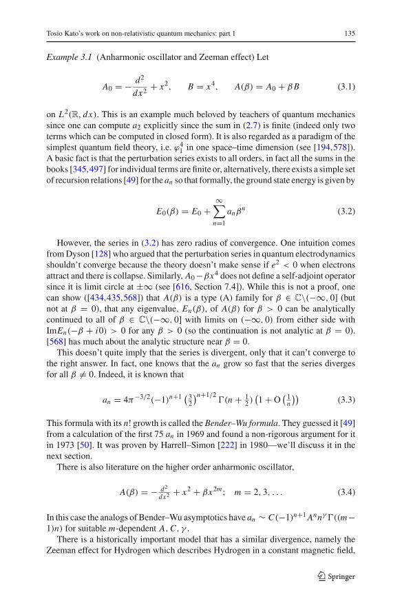
Example 3.1 (Anharmonic oscillator and Zeeman effect) Let
A0 = − d2
dx2+ x2, B = x4, A(β) = A0 + βB (3.1)
on L2(R, dx). This is an example much beloved by teachers of quantum mechanicssince one can compute a2 explicitly since the sum in (2.7) is finite (indeed only twoterms which can be computed in closed form). It is also regarded as a paradigm of thesimplest quantum field theory, i.e. ϕ4
1 in one space–time dimension (see [194,578]).A basic fact is that the perturbation series exists to all orders, in fact all the sums in thebooks [345,497] for individual terms are finite or, alternatively, there exists a simple setof recursion relations [49] for thean so that formally, the ground state energy is given by
E0(β) = E0 +∞∑
n=1
anβn (3.2)
However, the series in (3.2) has zero radius of convergence. One intuition comesfromDyson [128] who argued that the perturbation series in quantum electrodynamicsshouldn’t converge because the theory doesn’t make sense if e2 < 0 when electronsattract and there is collapse. Similarly, A0−βx4 does not define a self-adjoint operatorsince it is limit circle at ±∞ (see [616, Section 7.4]). While this is not a proof, onecan show ([434,435,568]) that A(β) is a type (A) family for β ∈ C\(−∞, 0] (butnot at β = 0), that any eigenvalue, En(β), of A(β) for β > 0 can be analyticallycontinued to all of β ∈ C\(−∞, 0] with limits on (−∞, 0) from either side withImEn(−β + i0) > 0 for any β > 0 (so the continuation is not analytic at β = 0).[568] has much about the analytic structure near β = 0.
This doesn’t quite imply that the series is divergent, only that it can’t converge tothe right answer. In fact, one knows that the an grow so fast that the series divergesfor all β �= 0. Indeed, it is known that
an = 4π−3/2(−1)n+1 ( 32
)n+1/2�(n + 1
2 )(1 + O
( 1n
))(3.3)
This formula with its n! growth is called the Bender–Wu formula. They guessed it [49]from a calculation of the first 75 an in 1969 and found a non-rigorous argument for itin 1973 [50]. It was proven by Harrell–Simon [222] in 1980—we’ll discuss it in thenext section.
There is also literature on the higher order anharmonic oscillator,
A(β) = − d2
dx2+ x2 + βx2m; m = 2, 3, . . . (3.4)
In this case the analogs of Bender–Wu asymptotics have an ∼ C(−1)n+1Annγ �((m−1)n) for suitable m-dependent A, C, γ .
There is a historically important model that has a similar divergence, namely theZeeman effect for Hydrogen which describes Hydrogen in a constant magnetic field,
123

136 B. Simon
B, which if B points in the z direction in r = (x, y, z) coordinates is given by theHamiltonian
A(B) = − 12� − 1
r + B2
8 (x2 + y2) + BLz (3.5)
where Lz is the z component of the angular momentum. For the ground state (whereLz = 0), one has that
E0(B) =∞∑
k=0
Ek B2k (3.6)
Avron [20] found a Bender–Wu type formula
Ek =(4
π
)5/2
(−1)k+1π−2k�
(2k + 3
2
)(1 + O
(1
k
))(3.7)
with a rigourous proof by Helffer–Sjöstrand [234]. In natural units, the magnetic fieldin early twentieth century laboratories was very small so lowest order perturbationtheory worked very well.
Example 3.2 (Autoionizing States of Two Electron Atoms) We further consider theHamiltonian A(1/Z)ofExample 2.1; see (2.17). For 1/Z = 0, A(0) is theHamiltonianof two uncoupled Hydrogen atoms so its eigenvalues are En,m = − 1
4n2− 1
4m2 , m, n =1, 2, . . .. The continuous spectrum starts at − 1
4 (for n = 1, m → ∞), so, for exam-ple, E2,2 at energy − 1
8 is an eigenvalue but not isolated, rather it is embedded inthe continuous spectrum on [− 1
4 ,∞). According to the physicist’s expectation, thiseigenvalue becomes a decaying state, where in a finite time, one electron drops to theground state and the other gets kicked out of the atom with the left over energy (i.e.− 1
8 − (− 14 ) = 1
8 ). For obvious reasons, these are called autoionizing states. Thesestates are actually seen as electron scattering resonances (under e+ He+ → e+ He+)or as photo ionization resonances (γ + He → He+ + e) called Auger resonances.
The situation has a complication we’ll ignore. The eigenvalue at energy − 18 has
multiplicity 16which one can reduce by using exchange, rotation and parity symmetry.For our purposes, it is useful to look at states with angular momentum 2 and azimuthalangular momentum 2 which are simple. In fact, there are states of unnatural parity(with angular momentum 1 but parity +); the continuous spectrum below − 1
16 is onlyof natural parity states so these unnatural parity eigenvalues are not embedded incontinuous spectrum and so they don’t disappear. There are actually 15 subspaceswith definite symmetry. In one, there is a doubly degenerate embedded eigenvalue, in3 an isolated eigenvalue and in 11 a simple embedded eigenvalue.
According to what is called the Wigner–Weisskopf theory [676], these scatteringresonances are complex poles of the S-matrix so the perturbed energy, E(β) has anon-zero imaginary part
Im E(β) = �(β)
2(3.8)
where � is the width of the resonance, i.e. |(E − E0) + i2�|−2 (the impact of a pure
pole to a quantum probability) has a distance � between the two points where it takeshalf its maximum value.
123

Tosio Kato’s work on non-relativistic quantum mechanics: part 1 137
Physicists argue that � = h/τ , where τ is the lifetime of the excited state.SometimesRayleigh–Schrödinger perturbation theory is called time–independent per-turbation theory because there is a formal textbook argument for computing lifetimesof embedded eigenvalues coupled to the continuum called time–dependent perturba-tion theory. In particular, the second order term in this theory is called the Fermi goldenrule, discussed, for example, in Landau–Lifshitz [407, pp. 140–153]. Simon [574] hasa compact way to write this second order term. If A(β) = A0+βB, A0ϕ0 = E0ϕ0 andP0(λ) is the spectral projection for A0 with {E0} removed, i.e. P0(λ) = fλ(A) where
fλ(x) ={1, x < λ, x �= E00, x ≥ λ, or x = E0
then
�(β) = �2β2 + O(β3) (3.9)
�2 = d
dλ〈Bϕ0, P0(λ)Bϕ0〉
∣∣∣∣λ=E0
(3.10)
The physics literature arguments for time–dependent perturbation theory are mathe-matically questionable and there were arguments about what the higher order termswere.
So this example causes lots of problems we’ll look at in Sect. 4: What is a reso-nance? What does the perturbation series have to do with the resonance energy? Canone mathematically justify the Fermi golden rule? What are the higher terms? Is therea convergent series?
In 1948, Friedrichs [172] considered a model (related to some earlier work of his[170]) with operators acting on L2([a, b], dx) ⊕ C with A0( f (x), ζ ) = (x f (x), ζ )
where a < 1 < b so that A0 has an embedded eigenvalue at E0 = 1. A(β) =A0 + βB where B is the rank two operator B( f (x), ζ ) = (ζh(x), 〈h, f 〉) for someh ∈ L2([a, b], dx). For suitable h and small β > 0, Friedrichs proved that A(β) hasno eigenvalues in spite of the fact of a first order perturbation term so the eigenvalueindeed dissolves. He did not discuss resonances but this was an early attempt to studya model which in his words “is clearly related to the Auger effect.”
Example 3.3 (Stark Effect) The Stark Hamiltonian describes the Hydrogen atom inan electric field. If F is the strength of the field and r = (x, y, z), then the operatoron L2(R3) has the form
A(F, Z) = −� − Z
r+ Fz (3.11)
We will primarily consider Z = 1. Schrödinger developed eigenvalue perturbationtheory [544] to apply it to the StarkHamiltonian. Aswith the Zeeman effect, laboratoryF’s are small so first or second order perturbation theory worked well when comparedto experiment and this was regarded as a great success.
Early on, Oppenheimer [470] pointed out that when F �= 0, A(F, Z) is not boundedbelow so that the A(F = 0, Z = 1) ground state is, as soon as F �= 0, swamped bycontinuous spectrum. Put differently, it becomes a finite lifetime state that decays. He
123

138 B. Simon
claimed to compute the lifetime but his calculation was wrong. There are argumentsabout whether his method was correct but eventually universal agreement that thecorrect asymptotics for the width, when Z = 1 and F is small, is that found byLanczos [404–406]:
�(F) ∼ 1
2Fexp
(− 1
6F
)(3.12)
which is usually called the Oppenheimer formula.In fact, one can prove that for any F �= 0, and any Z including Z = 0, A(F, Z) has
spectrum (−∞,∞) with infinite multiplicity, purely absolutely continuous spectrum.Titchmarsh [654] proved there are no embedded eigenvalues using the separability inparabolic coordinates we’ll use again below, Avron–Herbst [24] proved the existenceof wave operators from A(F, Z = 0) to A(F, Z) (wave operators are discussed inSect. 13 in Part 2) and Herbst [240] proved that those wave operators were unitaries,U , with U A(F, Z = 0)U−1 = A(F, Z).
In this regard, I should mention what I’ve called [588] Howland’s Razor after[258,259] and Occam’s Razor: “Resonances cannot be intrinsic to an abstract operatoron a Hilbert space but must involve additional structure.” For {A(F, 1)}F �=0 are allunitarily equivalent but we believe they have F-dependent resonance energies. We’lldiscuss the possible extra structures in the next section.
There is also a Bender–Wu type asymptotics
E(F) ∼∞∑
n=0
A2n F2n (3.13)
A2n = −62n+1(2π)−1(2n)!(1 + O
(1
n
))(3.14)
found formally by Herbst–Simon [245] and proven by Harrell–Simon [222]. Interest-ingly enough, there is a close connection between (3.14) and the original Bender–Wuformula (3.3) or rather its analog for
− d2
dx2+ x2 + βx4 − 1
4x2(3.15)
whose Bender–Wu formula was found by Banks, Bender and Wu [43]. Jacobi [276]discovered that a Coulomb plus linear potential in classical mechanics separates inelliptic coordinates and then Schwarzschild [546] and Epstein [141] extended this ideato old quantum theory. In particular, Epstein used parabolic coordinates. Schrödinger[544] and Epstein [142] extended this use of parabolic coordinates to the Hamiltonian(3.11). This separation was also used by Titchmarsh [647–651,654], Harrell–Simon[222] and by Graffi–Grecchi and collaborators [48,79,198,199,201,203,205].
Many of the same questions occur as for Example 3.2 which we’ll study in Sect. 4:What is a resonance? What is the meaning of the divergent perturbation series? Whatis the difference between (3.9) where �(β) = O(β2) and (3.12) where �(β) = O(βk)
for all k.
123

Tosio Kato’s work on non-relativistic quantum mechanics: part 1 139
Example 3.4 (Double Wells) The standard double well problem is
A(β) = − d2
dx2+ x2 − 2βx3 + β2x4 (3.16)
Writing
V (β, x) ≡ x2 − 2βx3 + β2x4
= x2(1 − xβ)2
= β2x2(β−1 − x)2
we see that if Uβ f (x) = f (β−1 − x) which is unitary, then Uβ A(β)U−1β = A(β).
If we let ϕ0(x) = π−1/4 exp(− 12 x2), then 〈ϕ0, A(β)ϕ0〉 = 1 + O(β2). But by sym-
metry, 〈Uβϕ0, A(β)Uβϕ0〉 = 1 + O(β2) while 〈ϕ0, Uβϕ0〉 and 〈A(β)ϕ0, Uβϕ0〉 areO(exp(−1/(4β2))), so very small. Thus, we see that while A(β = 0) has simpleeigenvalues at 2n + 1, n = 0, 1, 2, . . ., for β �= 0, A(β) has a least two eigenvaluesnear each En(β = 0).
So far as I know, Kato never discussed anything like double wells in print, but we’llsee shortly that it illuminates the meaning of stability, a subject that Kato was the firstto emphasize.
This model is closely related to the family on L2(Rν):
H(λ) = −� + λ2h(x) + λg(x) (3.17)
where h, g are C∞, g is bounded from below, h ≥ ε > 0 near ∞, h ≥ 0, h(x) = 0for only finitely many points and so that at those points the Hessian matrix ∂2h
∂xi ∂x jis
strictly positive definite. One is interested in eigenvalues of H(λ) as λ → ∞. Noticethat when g = 0, λ−2H(λ) = −λ−2� + h, so this is a quasi-classical (h → 0) limit.One can rephrase the double well as looking at − d2
dx2+ λ2x2(1 − x)2 by scaling of
space and energy (see Simon [601]). There is a considerable literature both on leadingasymptotics and on the exponential splitting of the two lowest eigenvalues—see, forexample, Simon [601,603] and Helffer–Sjöstrand [228–234]. We note that Witten[687] has a proof of the Morse inequalities that relies on this leading quasi-classicallimit (see also Cycon et al. [101]).
Example 3.5 Our last two examples, unlike the first four are neither well-known norheavily studied. They are from Kato’s first paper on perturbation of eigenvalues, a onepage letter to the editor of Progress of Theoretical Physics in 1948. Both examples,which also appear in his thesis [316], have A(β) = A0 + βB with
A0 = −〈ψ, ·〉ψ (3.18)
where ψ ∈ L2(R, dx) has ‖ψ‖2 = 1. He focuses on what happens to the simpleeigenvalue A0 has at E0 = −1.
123

140 B. Simon
In his first example, he takes B to be multiplication by x . This model is the poorman’s Stark effect. He doesn’t mention this connection in the paper but does in thethesis. He states without proof in the Note (but does have a proof in the thesis) that forβ �= 0, A(β) has no eigenvalues but has a purely continuous spectrum. He remarkedthat this example shows that the formal perturbation series may be quite meaninglesseven if no “divergence” occurs. In his later work, as we’ll see in Sect. 4, he did discussa possible significance of such series.
Example 3.6 A0 is given by (3.18) but now B is multiplication by x2. Kato statesand proves in his thesis that for β small and positive, A(β) has a simple eigenvaluenear E = −1. Kato proves this by direct calculation rather than the more generalstrong convergence method in his book which we discuss below. He then discussestwo explicit special ψ’s for which the first order term,
∫x2|ψ(x)|2dx , is infinite. For
ψ = c(1 + x2)−1/2, he finds (in the thesis; the paper only has the O(β1/2) term):
E(β) = −1 + β1/2 − 12β + 1
8β3/2 + O(β2). (3.19)
For ψ = c|x |1/2(1 + x2)−1 where the first order integral is only logarithmicallydivergent, he claims that
E(β) = −1 + β log(β) + O(β) (3.20)
The thesis but not the paper also discusses ψ = c(1 + x2)−1 where the first orderintegral is finite, he claims that
E(β) = −1 + β − 2β3/2 + O(β2) (3.21)
Kato is primarily a theoremprover and concept developer but occasionally he producesdetailed calculational results, often without details; we’ll discuss this further in Sect. 7.
This example is quite artificial but in his book [345], Kato has an example goingback to Rayleigh [492]
A(β) = − d2
dx2+ β
d4
dx4, β > 0 (3.22)
withϕ(0) = ϕ′(0) = ϕ(1) = ϕ′(1) = 0 (3.23)
boundary conditions. Clearly A(0) should have A(0) = − d2
dx2but the boundary con-
ditions (3.23) are too strong to get a self-adjoint operator. One can show that the rightboundary conditions for a strong limit are ϕ(0) = ϕ(1) = 0 and that
En(β) = n2π2[1 + 4β1/2 + O(β)
](3.24)
With these examples in mind, we turn to the general theory of asymptotic series.Recall [614, Section 15.1] that given a function β �→ f (β) on (0, B) and a sequence
123

Tosio Kato’s work on non-relativistic quantum mechanics: part 1 141
{an}∞n=0, we say that∑∞
n=0 anβn is an asymptotic series to order N if an only if
f (β) −N∑
n=0
anβn = o(βN ) (3.25)
Of course, if the series is asymptotic to order (N + 1), the right side of (3.25) can bereplaced by O(βN+1). We’ll mainly discuss series asymptotic to infinite order (i.e. toorder N for all N = 1, 2, . . .). It is easy to see that if f has an asymptotic series toinfinite order, then f determines all the coefficients an uniquely.
The function g(β) = 106 exp(−1/106β) has a zero asymptotic series. f (β) andf (β) + g(β) thus have the same asymptotic series so an asymptotic series tells usnothing about the value, f (β0), for a fixed β0. Typically however, for β0 small, a fewterms approximate f (β0) well but too many terms diverge. A good example is given[614, Table after (15.1.18)] for the error function Erfc(x) = 2√
π
∫∞x exp(−y2)dy for
which h(x) ≡ πx exp(x2)Erfc(x) has an asymptotic series in 1/x about x = ∞. Atx = 10, h(x) = .99507 . . .. The order N = 2 asymptotic series is good to 5 decimalplaces and for N = 108 to more than 22 decimal places. But for N = 1000, the seriesis about 10565. So it is interesting and important to know that a series is asymptoticbut if one knows the series and wants to know f , it is disappointing not to know more.
One often considers A(β) defined in a truncated sector {β ∈ C | 0 < |β| <
B, | argβ| < A} and demands (3.25) (with βN in the error replaced by |β|N ) inthe whole sector.
In his thesis, Kato [316] only considered A(β) = A0 + βB with A ≥ 0, B ≥ 0where A(β) is self-adjoint (with a suitable interpretation of the sum). He used whatare now called Temple–Kato inequalities to obtain asymptotic series to all orders in[316,322]. We discuss this approach in Sect. 6 below.
About the same time, Titchmarsh started a series of papers [647–651,654] on eigen-values of second order differential equations including asymptotic perturbation resultsfor A(β) = − d2
dx2+ V (x) + βW (x) on L2(R, dx) (or L2((0,∞), dx) with a bound-
ary condition at x = 0). Typically both V (x) and W (x) go to infinity as |x | → ∞(so the spectra are discrete) and W goes to ∞ faster (so analytic perturbation theoryfails; think V (x) = x2, W (x) = x4). His work relied heavily on ODE techniques.They have overlap of applicability with Kato’s operator theoretic approach, but Kato’smethod is more broadly applicable.
In his book, Kato totally changed his approach to be able to say something aboutthe Banach space (and also non-self-adjoint operators in Hilbert space) so he couldn’tuse the Temple–Kato inequality which relies on the spectral theorem. There is someoverlap of this work from his book andwork of Huet [260], Kramer [388,389], Krieger[392] and Simon [568].
Central to Kato’s approach is the notion of strong resolvent convergence and ofstability. Kato often discusses this for sequences An converging to A in some senseas n → ∞; for our purposes here, it is more natural to consider A(β) depending ona positive real parameter as β ↓ 0. To avoid various technicalities, we’ll also focus
123

142 B. Simon
initially on the self-adjoint case were there are a priori bounds on (B − z)−1 forz ∈ C\R, although we’ll consider some non-self-adjoint operators later.
For (possibly unbounded) self-adjoint {A(β)}0<β<B and self-adjoint A0, we saythat A(β) converges in strong resolvent sense (srs) if and only if for all z ∈ C\R, wehave that (A(β) − z)−1 → (A0 − z)−1 in the strong (bounded) operator topology.Here is a theorem, going back to Rellich [504–508, Part 2] describing some resultscritical for asymptotic perturbation theory:
Theorem 3.7 Let A0 be self-adjoint and {A(β)}0<β<B a family of self-adjoint oper-ators on a Hilbert space, H.
(a) If D ⊂ H is a dense subspace with D ⊂ D(A0) and for all β ∈ (0, B), D ⊂D(A(β)), and ifD is a core for A0 and for all ϕ ∈ D, we have that A(β)ϕ → A0ϕ
as β ↓ 0, then A(β) → A0 in srs.(b) If a, b ∈ R are not eigenvalues of A0 and A(β) → A0 in srs, then
P(a,b)(A(β))s→ P(a,b)(A0) (3.26)
where P�(B) is the spectral projection for B associated to the set � ⊂ R [616,Chapter 5 and Section 7.2]
Proof (a) follows from a simple use of the second resolvent formula; see [616, The-orem 7.2.11]. For (b), one first proves (3.26) when P(a,b) is replaced by a continuousfunction [616, Theorem 7.2.10] and then approximates P(a,b) with continuous func-tions [616, Problem 7.2.5]. ��Remark Before leaving the subject of abstract srs results, we should mention tworesults known as the Trotter–Kato theorem (Kato’s ultimate Trotter product formula,the subject of Sect. 18, is also sometimes called theTrotter–Kato theorem).One versionsays that if An and A are generators of contraction semigroups on a Banach space, X ,then e−t An
s→ e−t A for all t > 0 if and only if for one (or for all)λwithRe (λ) > 0, onehas (An +λ)−1 s→ (A+λ)−1. Related, sometimes part of the statement of the theorem,is that one doesn’t require A to exist a priori but only that for some λ in the open halfplane that (An + λ)−1 have a strong limit whose range is dense. The basic theoremis then due to Trotter [655] in his thesis (written under the direction of Feller, whoseinterest in semigroups was motivated by Markov processes). Kato’s name is often onthe theorem because he clarified an obscure point in this second version [331]. Thistheorem has also been called the Trotter–Kato–Neveu or Trotter–Kato–Neveu–Kurtz–Sova theorem after related contributions by these authors [402,403,466,622]. Thereis another related result of this genre sometimes called the Trotter–Kato theorem. Itsays that if An is a family of self-adjoint operators, they have a srs limit for some A ifand only if (An − z)−1 has a strong limit with dense range for one z in C+ and one zin C−.
Returning to perturbation theory, Kato introduced and developed the key notionof stability. Let {A(β)}0<β<B (or β in a sector) be a family of closed operators in aBanach space, X . Let A0 be a closed operator so that as β ↓ 0, A(β) converges to A0
123

Tosio Kato’s work on non-relativistic quantum mechanics: part 1 143
in some sense. Let E0 be an isolated, discrete, eigenvalue of A0. We say that E0 isstable if there exists ε > 0 so that σ(A0) ∩ {z | |z − E0| ≤ ε} = {E0} and so that
(a) |β| < B and |z − E0| = ε ⇒ z /∈ σ(A(β)) and for each ϕ ∈ X
limβ↓0(A(β) − z)−1ϕ = (A0 − z)−1ϕ (3.27)
uniformly in {z | |z − E0| = ε}(b) If P(β) is given by (2.1) with A = A(β) and with� the counterclockwise circle
indicated at the end of (a), then, for all β small, we have that
dim ran P(β) = dim ran P(0) (3.28)
The uniform strong convergence in (a) implies that
P(β)s→ P(0) (3.29)
In the self-adjoint case, even without (a), if A(β) → A0 in srs, then
P(E0−ε,E0+ε)(A(β))s→ P{E0}(A0) (3.30)
for ε small if E0 is in the discrete spectrum of A0. P �→ dim ran P is continuous inthe topology of norm convergence but it is only lower semicontinuous in the topol-ogy of strong operator convergence. For example, if Pn is the rank one projectiononto multiples of the nth element of an orthonormal basis, then Pn
s→ 0. The lowersemicontinuity says that
Pns→ P∞ ⇒ dim ran P∞ ≤ lim inf dim ran Pn (3.31)
Kato was well aware that equality might not hold on the right side of (3.31) forexamples of relevance to physics—amain example that he mentions is the Stark effectwhere the right side is infinite. Double wells show that even if (a) above holds, (b)may fail. Simon [601] describes an extension of stability for multiple well problems.
There are two main ways that one can prove stability in cases where it is true. Oneis to note that if A(β) ≥ A0 as happens if
A(β) = A0 + βB (3.32)
and B ≥ 0, then dim ran P(−∞,a)(A(β)) ≤ dim ran P(−∞,a)(A0). This and (3.31)implies stability for E0 below the bottom of the essential spectrum for A0. This is thetypical approach that Kato uses in several places.
The second way one can have stability is illustrated by
Example 3.8 (Example 3.1 (revisited)) One might have the impression that regularperturbation theory is associated with norm continuity of resolvents and spectral pro-jections and asymptotic perturbation theory always only strong convergence. While
123

144 B. Simon
there is some truth to this, Simon [568] found the surprising fact that even in situationswhere perturbation theory diverges, one can have norm convergence of resolvents ina sector. One starts by noting that with p = 1
id
dx , one has that
(p2 + W )2 = p4 + W 2 + p2W + W p2
= p4 + W 2 + 2pW p + [p, [p, W ]]= p4 + W 2 + 2pW p − W ′′
≥ 12W 2 − c
if W ′′ ≤ 12W 2 + c and W ≥ 0. In this way, one sees that for positive constants c and d
‖(p2 + x2 + βx4)ϕ‖2 + c‖ϕ‖2 ≥ d[‖x2ϕ‖2 + β2‖x4ϕ‖2
](3.33)
which is called a quadratic estimate. This, in turn, implies that ‖x2(p2 + x2 + 1)−1‖and ‖(p2 + x2 + βx4 + 1)−1x2‖ are bounded so that
‖(p2 + x2 + βx4 + 1)−1 − (p2 + x2 + 1)−1‖= β‖(p2 + x2 + βx4 + 1)−1x4(p2 + x2 + 1)−1‖≤ β‖(p2 + x2 + βx4 + 1)−1x2‖‖x2(p2 + x2 + 1)−1‖
is O(β) → 0 in norm. This implies stability by a simple argument.A similar argument works for p2 + γ x2 + βx4 for any γ ∈ ∂D\{−1} so using
scaling and the ideas below, one proves that for each n, the nth eigenvalue, En(β), ofp2+x2+βx4 has an asymptotic series in each sector {β | 0 < |β| < BA; | argβ| < A}so long as A ∈ (0, 3π
2 ) [568].The above argument doesn’t work for βx2m; m > 2 but by using that ‖βx2m(p2 +
x2+βx2m +1)−1‖ is bounded, one sees that the normof the difference of the resolventsis O(β1/m) which also goes to zero.
To state results on asymptotic series, we focus on getting series for all orders.Kato [345] is interested mainly in first and second order, so he needs much weakerhypotheses. LetC ≥ 1be a self-adjoint operator on aHilbert space,H. Then D∞(C) ≡∩n≥0D(Cn) is a countably normed Fréchet space with the norms ‖ϕ‖n ≡ ‖Cnϕ‖H(see [612, Section 6.1]). A densely defined operator, X , on D∞(C) is continuous inthe Fréchet topology if and only if for all m, there is k(m) and cm so that Dk(m)(C) ⊂D(X), X
[Dk(m)(C)
] ⊂ Dm(C) and ‖Xϕ‖m ≤ cm‖ϕ‖k(m). Typically, for some �,k(m) can be chosen to be m + �.
Theorem 3.9 Let C ≥ 1 be a self-adjoint operator on a Hilbert space, H. Let{A(β)}0≤β<B be a family of closed operators with E0 a simple isolated eigenvalueof A0 ≡ A(0). Suppose that D∞(C) ∩ D(A0) ⊂ D(A(β)) for all β. Let V be anoperator with D∞(C) ∩ D(A0) ⊂ D(V ) so that for ϕ ∈ D∞(C) ∩ D(A0), we havethat
A(β)ϕ = (A0 + βV )ϕ (3.34)
123
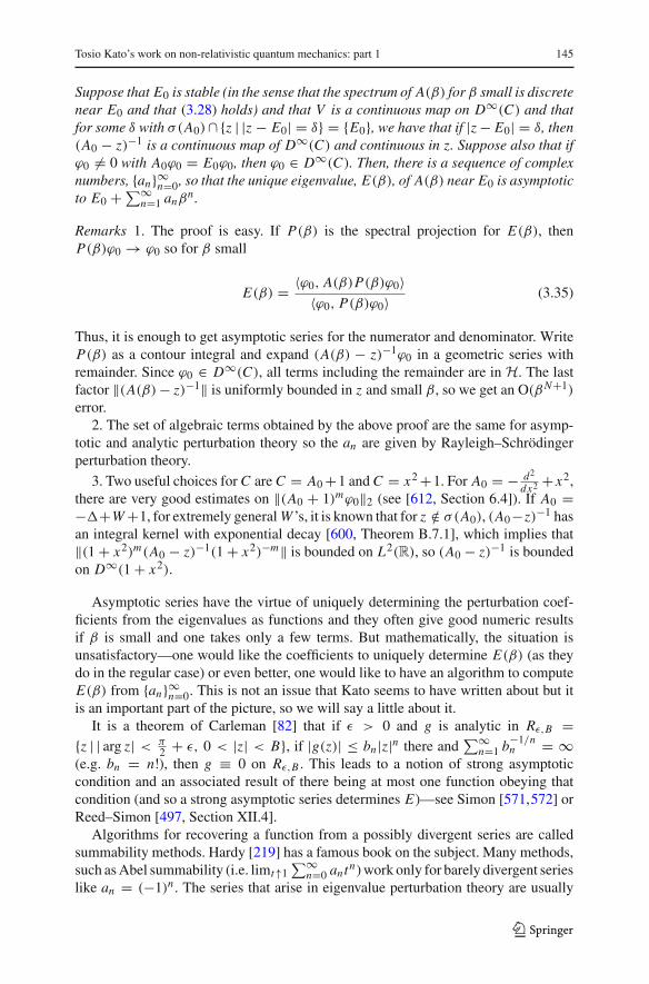
Tosio Kato’s work on non-relativistic quantum mechanics: part 1 145
Suppose that E0 is stable (in the sense that the spectrum of A(β) for β small is discretenear E0 and that (3.28) holds) and that V is a continuous map on D∞(C) and thatfor some δ with σ(A0)∩ {z | |z − E0| = δ} = {E0}, we have that if |z − E0| = δ, then(A0 − z)−1 is a continuous map of D∞(C) and continuous in z. Suppose also that ifϕ0 �= 0 with A0ϕ0 = E0ϕ0, then ϕ0 ∈ D∞(C). Then, there is a sequence of complexnumbers, {an}∞n=0, so that the unique eigenvalue, E(β), of A(β) near E0 is asymptoticto E0 +∑∞
n=1 anβn.
Remarks 1. The proof is easy. If P(β) is the spectral projection for E(β), thenP(β)ϕ0 → ϕ0 so for β small
E(β) = 〈ϕ0, A(β)P(β)ϕ0〉〈ϕ0, P(β)ϕ0〉 (3.35)
Thus, it is enough to get asymptotic series for the numerator and denominator. WriteP(β) as a contour integral and expand (A(β) − z)−1ϕ0 in a geometric series withremainder. Since ϕ0 ∈ D∞(C), all terms including the remainder are in H. The lastfactor ‖(A(β) − z)−1‖ is uniformly bounded in z and small β, so we get an O(βN+1)
error.2. The set of algebraic terms obtained by the above proof are the same for asymp-
totic and analytic perturbation theory so the an are given by Rayleigh–Schrödingerperturbation theory.
3. Two useful choices for C are C = A0+1 and C = x2+1. For A0 = − d2
dx2+ x2,
there are very good estimates on ‖(A0 + 1)mϕ0‖2 (see [612, Section 6.4]). If A0 =−�+W +1, for extremely general W ’s, it is known that for z /∈ σ(A0), (A0−z)−1 hasan integral kernel with exponential decay [600, Theorem B.7.1], which implies that‖(1 + x2)m(A0 − z)−1(1 + x2)−m‖ is bounded on L2(R), so (A0 − z)−1 is boundedon D∞(1 + x2).
Asymptotic series have the virtue of uniquely determining the perturbation coef-ficients from the eigenvalues as functions and they often give good numeric resultsif β is small and one takes only a few terms. But mathematically, the situation isunsatisfactory—one would like the coefficients to uniquely determine E(β) (as theydo in the regular case) or even better, one would like to have an algorithm to computeE(β) from {an}∞n=0. This is not an issue that Kato seems to have written about but itis an important part of the picture, so we will say a little about it.
It is a theorem of Carleman [82] that if ε > 0 and g is analytic in Rε,B ={z | | arg z| < π
2 + ε, 0 < |z| < B}, if |g(z)| ≤ bn|z|n there and∑∞
n=1 b−1/nn = ∞
(e.g. bn = n!), then g ≡ 0 on Rε,B . This leads to a notion of strong asymptoticcondition and an associated result of there being at most one function obeying thatcondition (and so a strong asymptotic series determines E)—see Simon [571,572] orReed–Simon [497, Section XII.4].
Algorithms for recovering a function from a possibly divergent series are calledsummability methods. Hardy [219] has a famous book on the subject. Many methods,such asAbel summability (i.e. limt↑1
∑∞n=0 antn)work only for barely divergent series
like an = (−1)n . The series that arise in eigenvalue perturbation theory are usually
123

146 B. Simon
badly divergent but, fortunately, there are some methods that work even in that case.Two that have been shown to work for suitable eigenvalue problems are Padé andBorel summability.
The ordinary approximates for a power series are by the polynomials obtained bytruncating the power series. If instead, one uses rational functions, one gets Padé,aka Hermite–Padé, approximates (they were formally introduced by Padé [473] inhis thesis—Hermite, who was Padé’s advisor, introduced them earlier in the specialcase of the exponential function [246]). Specifically, given a formal power series,∑∞
n=0 anzn , the Padé approximates, f [N ,M], are given by
f [N ,M](z) = P [N ,M](z)Q[N ,M](z)
; deg P [N ,M] = M, deg Q[N ,M] = N (3.36)
f [N ,M](z) −N+M∑n=0
anzn = O(
zN+M+1)
(3.37)
In (3.37), f [N ,M] has (N + 1 + M + 1) − 1 parameters as does the sum. Thus(3.36)/(3.37) is (N + M + 1) equations in the coefficients of P and Q. So long ascertain determinants formed from {an}N+M
n=0 are non-zero, there is a unique solution,f [N ,M](z). For more on Padé approximates, see Baker [35–37].The othermethod is calledBorel summability, introduced byBorel [65]. Themethod
requires that|an| ≤ ABnn! (3.38)
for some A, B and all n. If that is so, one forms the Borel transform
g(w) =∞∑
n=0
an
n! wn (3.39)
which defines an analytic function in {w | |w| < B−1}. One supposes that g has ananalytic continuation to a neighborhood of [0,∞) and defines for z real and positive
f (z) =∫ ∞
0e−ag(az)da (3.40)
Since∫∞0 e−aanda = n!, formally f (z) is
∑∞n=0 anzn . For this method to work, g
has to have an analytic continuation so that the integral in (3.40) converges.As far as Padé is concerned, a major result involves sequences, {an}∞n=0, called
series of Stieltjes which have the form
an = (−1)n∫ ∞
0xndμ(x) (3.41)
123

Tosio Kato’s work on non-relativistic quantum mechanics: part 1 147
for some positive measure dμ on [0,∞) with all moments finite. The associatedStieltjes transform of μ
f (z) =∫ ∞
0
dμ(x)
1 + xz(3.42)
is defined and analytic in z ∈ C\(−∞, 0]. Expanding (1 + xz)−1 in a geometricseries with remainder, one sees that in every sector {z | | arg z| < π − ε} with ε > 0,∑∞
0 anzn is an asymptotic series for f . Here is the big theorem for such series:
Theorem 3.10 If {an}∞n=0 is a series of Stieltjes, then for each j ∈ Z, the diagonalPadé approximates, f [N ,N+ j](z), converge as N → ∞ for all z ∈ C\[0,∞) toa function f j (z) given by (3.42) with μ replaced by μ j which obeys (3.41) (withμ = μ j ). The f j are either all equal or all different depending on whether (3.41) hasa unique solution, μ, or not.
The result is due to Stieltjes [626,627]who discussed solutions of themoment prob-lem (3.40) but not Padé approximates. Rather following ideas of Jacobi, Chebyshevand Markov, he discussed continued fractions expansions
α1
z + β1 + α2
z + β3 + α3
. . .
for the Stieltjes transform. These are the f [N+1,N ](z) and his convergence resultsimply the theorem. For details, see Baker [36] or Simon [616, Section 7.7].
It follows from results of Loeffel et al. [434,435] that if Em(β) is an eigenvalue ofp2 + x2 + βx4 for β ∈ [0,∞), then Em(β) has an analytic continuation to C\[0,∞)
with a positive imaginary part in the upper half plane. Results of Simon [568] implythat |Em(β)| ≤ C(1+|β|)1/3. A Cauchy integral formula then implies that (Em(0)−Em(β))/β has a representation of the form (3.42). Thus, by [435], the diagonal Padéapproximates converge. Moreover, it is a fact (related to the above mentioned theoremof Carleman) that if {an}∞n=0 is the set of moments of a measure on [0,∞) with|an| ≤ C Dn(kn)!with k ≤ 2, then the solution to the moment problem is unique [612,Problem 5.6.2]. This implies that for the x4 anharmonic oscillator, the diagonal Padéapproximates converge to the eigenvalues. The same is true for the x6 oscillator butfor the x8 oscillator, it is known (Graffi–Grecchi [200]) that, while the diagonal Padéapproximates converge, they have different limits and none is the actual eigenvalue!
The key convergence result for Borel sums is a theorem ofWatson [673]; see Hardy[219] for a proof:
Theorem 3.11 Let � ∈ (π2 , 3π
2
)and B > 0. Define
� = {z | 0 < |z| < B, | arg z| < �} (3.43)
� = {z | 0 < |z| < B, | arg z| < � − π2 } (3.44)
� = {w | w �= 0, | argw| < � − π2 } (3.45)
123

148 B. Simon
Suppose that {an}∞n=0 is given and that f is analytic in � and obeys
∣∣∣∣∣ f (z) −N∑
n=0
anzn
∣∣∣∣∣ ≤ AC N+1(N + 1)! (3.46)
on � for all N . Define
g(w) =∞∑
n=0
an
n! wn; |w| < C−1 (3.47)
Then g(w) has an analytic continuation to � and for all z ∈ �, we have that
f (z) =∫ ∞
0e−ag(az)da (3.48)
Graffi–Grecchi–Simon [204] proved that this theorem is applicable to the x4 anhar-monic oscillator. They did numeric calculations making an unjustified use of Padéapproximation to analytically continue g to all of [0,∞) and found more rapid con-vergence than Padé on the original series. By conformally mapping a subset of theunion ofD and� containing [0,∞) onto the disk, one can do the analytic continuationby summing a mapped power series and so do numerics without an unjustified Padé;see Hirsbrunner and Loeffel [249].
There is a higher order Borel summation where one picks m = 2, 3, . . ., � ∈(mπ2 , 3mπ
2
)and replaces � − π
2 in (3.44) by � − mπ2 , (N + 1)! in (3.46) is replaced
by [m(N + 1)]!, n! in (3.47) by (mn)! and (3.48) by
f (z) =∫ ∞
0e−a1/m
g(za)a
(1m −1
)da (3.49)
They showed [204] that the x2(m+1) oscillator is modified m-Borel summable.Avron–Herbst–Simon [25–28, Part III] proved that for theZeeman effect in arbitrary
atoms, the perturbation series of the discrete eigenvalues is Borel summable. TheSchwinger functions of various quantum field theories have been proven to have Borelsummable Feynman perturbation series: P(φ)2 [133], φ4
3 [438], Y2 [513,514], Y3[439].
In general, Padé summability is hard to prove because it requires global informa-tion, so it has been proven to work only in very limited situations (for example ahigher dimensional quartic anharmonic oscillator is known to be Borel summable butnothing about Padé is known). Clearly, when it can be proven, Borel summability isan important improvement over the mere asymptotic series that concerned Kato.
Before leaving asymptotic perturbation theory, we mention a striking example ofHerbst–Simon [243]
A(β) = − d2
dx2+ x2 − 1 + β2x4 + 2βx3 − 2βx
123

Tosio Kato’s work on non-relativistic quantum mechanics: part 1 149
If E0(β) is the lowest eigenvalue, they prove that for all small, non-zero positive β
0 < E0(β) < C exp(−Dβ−2)
Thus E0(β) has∑∞
n=0 anβn as asymptotic series where an ≡ 0. The asymptotic seriesconverges but, since E0 is strictly positive, it converges to the wrong answer!
4 Eigenvalue perturbation theory, III: spectral concentration
Starting around 1950, Kato [316] and Titchmarsh [647–651,654] considered what theperturbation series might mean for a problem like the Stark problem where a discreteeigenvalue is swallowed by continuous spectrum as soon as the perturbation is turnedon. Titchmarsh looked mainly at ODEs; in particular, he looked at what has come tobe called the Titchmarsh problem, (g ≥ − 1
4 , z > 0)
h(g, z, f ) = − d2
dx2+ g
x2− z
x− f x (4.1)
(for some values of g, one needs a boundary condition at x = 0). Kato used operatortheory techniques and studied Examples 3.3 and 3.5.
Titchmarsh proved that the Green’s kernel for h, originally defined for energiesin C+, had a continuation onto the lower half plane with a pole near the discreteeigenvalues of h(g, z, f ) and he identified the real part of the pole with perturbationtheory up to second order. He conjectured that the imaginary part of the pole wasexponentially small in 1/ f . He then showed in a certain sense that the spectrum ofh(g, z, f �= 0) as f ↓ 0 concentrated near the real parts of his poles [647–651, PartV].
Kato discussed things in terms of what he called pseudo-eigenvalues and pseudo-eigenvectors.He later realized that these notions imply a concentration of spectrum likethat used by Titchmarsh. In his book [345], he emphasized what he formally definedas spectral concentration and linked the two approaches. In this section, I’ll begin bydefining spectral concentration and then prove, following Kato, that it is implied bythe existence of pseudo-eigenvectors. Finally, I’ll discuss the complex scaling theoryof resonances and how it extends and illuminates the theory of spectral concentration.
Consider first the case where A(β) converges to A0 as β ↓ 0 in srs and E0 is adiscrete simple eigenvalue of A0. Let T be a closed interval with σ(A0) ∩ T = {E0}.By Theorem 3.7, for any ε > 0, we have that PT \(E0−ε,E0+ε)(A(β))
s→ 0. Thus, in asense, the spectrum of A(β) in T is concentrated near E0. In the above, if we couldreplace (E0−ε, E0+ε) by (E0+a1β −β3/2, E0+a1β +β3/2), we’d be able to claimthat the spectrum was concentrated near E0 + a1β in a way that would determine a1.
Taking into account that we may want to also have T shrink in cases like Example3.2, we make the following definition. Let T (β), S(β) be Borel sets in R given for0 < β < B so that if 0 < β ′ < β, then T (β ′) ⊂ T (β), S(β ′) ⊂ S(β) and so thatfor all β, S(β) ⊂ T (β). We say that the spectrum of A(β) in T (β) is asymptotically
concentrated in S(β) if and only if PT (β)\S(β)s→ 0.
123

150 B. Simon
If E0 is a simple eigenvalue of A0 and {a j }Nj=1 are real numbers,we say the spectrum
near E0 is asymptotically concentrated near E0 +∑Nj=0 a jβ
j if there exist positive
functions f and g obeying f (β) → 0, f (β)/β → ∞, g(β)/βN → 0 as β ↓ 0 sothat the spectrum of A(β) in (E0 − f (β), E0 + f (β)) is asymptotically concentratedin (E0+∑N
j=0 a jβj −g(β), E0+∑N
j=0 a jβj +g(β)). It is easy to see if that happens,
it determines the a j , j = 1, . . . , n.Kato’s thesis [316] introduced the notion of N th order pseudo-eigenvectors and
pseudo-eigenvalues. In later usage, this is a pair of functions, ϕ(β) and λ(β), on(0, B) with values inH and R so that
ϕ(β) ∈ D(A(β)), ‖ϕ(β)‖ = 1, λ(β) → E0 (4.2)
‖(A(β) − λ(β))ϕ(β)‖ = o(βN ) (4.3)
Conley–Rejto [95] and Riddell [515] (Riddell was a student of Kato and this paperwas based on his PhD. thesis) proved the following
Theorem 4.1 If E0 is a simple isolated eigenvalue of A0 and (ϕ(β), λ(β)) are an Nthorder pseudo-eigenvector and pseudo-eigenvalue so that as β ↓ 0, we have that
(1 − PE0(A0))ϕ(β) → 0 (4.4)
Then there exists g(β) = o(βN ) and d > 0 so that the spectrum of A(β) in (E0 −d, E0 + d) is concentrated in (λ(β) − g(β), λ(β) + g(β)).
Remarks 1. Riddell also has a converse.2. Both papers consider the situation where E0 has multiplicity k < ∞ and there
are k orthonormal pairs obeying (4.3) and they prove spectral concentration on aunion of k intervals of size o(βN ) about the λ j .
3. The proof isn’t hard. One picks g(β) = o(βN ) so that ‖(A(β) − λ(β))ϕ(β)‖/g(β) → 0. This implies that if Q(β) = P(λ(β)−g(β),λ(β)+g(β))(A(β)), then ‖(1 −Q(β))ϕ(β)‖ → 0. By (4.4), this implies that
‖Q(β) − PE0(A0)‖ → 0 (4.5)
If d < dist(E0, σ (A)\{E0}), Theorem 3.7 implies that P(E0−d,E0+d)(A(β))ψ →PE0(A0)ψ for anyψ . Thus by (4.5),
[P(E0−d,E0+d)(A(β)) − Q(β)
]ψ → 0which
is the required spectral concentration
These ideas were used by Friedrichs and Rejto [175] to prove spectral concentrationinExample 3.5 (i.e. A0 of rank 1 and B multiplication by x). They assumed the functionψ(x) of (3.18) is strictly positive on R and Hölder continuous and prove that A(β)
has no point eigenvalues and has a weak spectral concentration (of order β p for some0 < p < 1). Riddell [515] proved spectral concentration to all orders for the Starkeffect for Hydrogen using pseudo-eigenvectors and Rejto [501,502] proved the analogfor Helium (see below for more on spectral concentration for the Stark effect).
Veselic [661] systematized and simplified the results in Theorem 4.1 and applied itto certainmodels (not linear inβ)where A0 has a discrete eigenvaluewhile A(β) has no
123

Tosio Kato’s work on non-relativistic quantum mechanics: part 1 151
eigenvalue due to tunnelling through a barrier. An example is A(β) = − d2
dx2+V (x, β)
whereV (x, β) = V0(x) − (1 − e−βx ) (4.6)
V0 goes to zero at infinity and is such that A0 has a single negative eigenvalue at − 12 .
Thus A(β) has essential spectrum [−1,∞) and instantaneously the discrete eigenvalueis swamped in continuous spectrum. There is a barrier of size β−1 trapping the initialbound state. Veselic proved spectral concentration.
As noted Titchmarsh related spectral concentration to second sheet poles of Green’sfunctions for certain differential operators. This theme was developed by James How-land, a student of Kato, in 5 papers [255–259]. Howland discussed two situations. Onewas where A0 was finite rank and whose non-zero eigenvalues are washed away muchlike Example 3.5. The other was where A0 has eigenvalues embedded in continuousspectrum and B is finite rank, so related to the Friedrichs model mentioned at the endof Example 3.2.
In both cases, there is a finite dimensional space, V , where the finite rank operatorlives and Howland considered {〈ϕ, (A(β) − z)−1ψ〉, | ϕ,ψ ∈ V} and proved (undersuitable conditions) that these functions initially defined on C+ have meromorphiccontinuations through R into a neighborhood of E0, a finite multiplicity eigenvalue ofA0. These continuations had second sheet poles at E j (β) converging as β ↓ 0 to E0.The number of poles is typically the multiplicity of E0 as an eigenvalue of A0.
In the case where A0 has a discrete eigenvalue, Howland showed that Im E(β) =O(β�) for all � and was able to use this to prove spectral concentration to allorders. But in cases where A0 had an embedded eigenvalue, it was typically truethat Im E(β) = akβ
k + o(βk) for some k and some ak < 0; indeed Howland oftenproved a Fermi golden rule with a2 �= 0. In that case, he showed there was spectralconcentration of order k − 1 but not k so spectral concentration couldn’t specify aperturbation series to all orders.
Howland also discovered that even when A0 and B were self-adjoint, an eigenvaluecould turn into a second order pole whose perturbation series could have non-trivialfractional power series in the asymptotic expression, i.e. Rellich’s theorem fails forresonance energies.
Howland also introduced what I’ve called Howland’s razor (see the discussion ofExample 3.3) and he gave one possible answer: it often happened that the embeddedeigenvalue turned into a resonance, i.e. second sheet pole, for real values of β butfor suitable complex β, it was a pole in C+ and so a normal discrete eigenvalue ofA(β). Thus the resonance energy could be interpreted as the analytic continuation ofa perturbed eigenvalue.
Perhaps the most successful approach to the study of resonances, one that handlesproblems in atomic physics like Examples 3.2 and 3.3, is the method of complexscaling, initially called dilation or dilatation analyticity (the name change to complexscaling was by quantum chemists when they took up the method for numerical calcu-lation of molecular resonances). The idea appeared initially in a technical appendixof a never published note by J. M. Combes who realized the potential of this idea andthen published papers with coauthors: Aguilar–Combes [6] on the two body problemand Balslev–Combes [42] on N -body problems (Eric Balslev was Kato’s first Berke-
123

152 B. Simon
ley student); see Simon [573] for extensions and simplifications and [497, SectionsXIII.10 and XII.6] for a textbook presentation. Combes and collaborators knew thatthe formalism, which they used to prove the absence of singular continuous spectrum,provided a possible definition of a resonance. It was Simon [574] who realized that theformalism was ideal for studying eigenvalues embedded in the continuous spectrumlike autoionizing states. We will not discuss an extension needed for molecules in thelimit of infinite nuclear masses where one uses exterior complex scaling or a closevariant, see Simon [594], Hunziker [263] and Gérard [187].
We begin with the two body case. On L2(Rν, dνx), let U (θ), θ ∈ R be the set ofreal scalings:
(U (θ) f )(r) = eνθ/2 f (eθ r) (4.7)
which defines a unitary group. If H = −� + V (r), then
H(θ) ≡ U (θ)HU (θ)−1 = −e−2θ� + V (eθ r) (4.8)
The first term, H0(θ), can be analytically continued and
σ(H0(θ)) = {z ∈ C\{0} | arg z = −2Im θ} ∪ {0} ≡ Sθ (4.9)
Suppose that θ �→ V (eθ r) has an analytic continuation as a compact operator fromD(−�) to L2(Rν) for |Im θ | < �0 as happens for V (r) = r−α (0 < α < 2; includingα = 1, i.e. Coulomb) for all �0 or for V (r) = e−γ r for �0 = π
2 . Such V ’s are calleddilation analytic. Then H(θ) is a type (A) analytic family on the strip of width 2�0about R. For any θ , the essential spectrum of H(θ) is Sθ .
Discrete eigenvalues are given by analytic functions, E j (θ). Since changing Re θ
provides unitarily equivalent H ’s, E j (θ) is constant under changes of Re θ , so constantby analyticity. We conclude that so long as discrete eigenvalues avoid Sθ , they remaindiscrete eigenvalues of H(θ). In particular, negative eigenvalues of H are eigenval-ues of H(θ) if |Im θ | < π
2 . An additional argument shows that embedded positiveeigenvalues become discrete eigenvalues of H(θ) for Im θ ∈ (0, π
2 ).By this persistence, H(θ) for θ with Im θ ∈ (0, π
2 ), there can’t be any eigenvaluesin {z | arg z ∈ (0, 2π − 2Im θ)\{−π}} (for taking θ back to zero would result innon-real eigenvalues of H ) but there isn’t any reason there can’t be for z with arg z ∈(−2Im z, 0). That is, moving Im θ can uncover eigenvalues in C− which we interpretas resonances (but see the discussion below).
Using techniques from N -body quantum theory (essentially the HVZ theorem tobe discussed in Sect. 11; we’ll use notation from that section below), one can similarlyanalyze N -body Hamiltonians with center of mass removed when all the Vi j aredilation analytic. The spectrum of H(θ) with θ not real looks like that in Fig. 1.
If C is a non-trivial cluster decomposition of {1, . . . , N }, C = {C1, . . . , Ck} andh(C j ) is the internal Hamiltonian of C j , the set of E1 + · · · + Ek where E j is aneigenvalue of h(C j ) is called the set of thresholds (if some C� has one particle, thenh(C�) is the zero operator on C and E� = 0). It can be shown [42,573] that the set,�, of all thresholds (running over all non-trivial cluster decompositions) is a closedcountable set and that for 0 < Im θ < �0 < π
2 , one has that
123

Tosio Kato’s work on non-relativistic quantum mechanics: part 1 153
Fig. 1 The Spectrum of H(θ) (a) Discrete eigenvalue of H (b) Continuum-embedded eigenvalues (c)Thresholds of H (d) Resonance eigenvalues (e) Complex thresholds
σess(H(θ)) =⋃
λ∈�(θ)
λ + Sθ (4.10)
Here �(θ) includes some complex λ where the E j are resonance eigenvalues ofh(C j , θ).
Example 3.2 revisited. (following [574]) The thresholds are{− 1
4n2
}∞n=1
so the eigen-
value at E2,2 = − 18 is not a threshold. Thus it is an isolated eigenvalue of A(1/Z , 0, θ)
if−iθ ∈ (0, π2 ). It follows that theKato–Rellich theory applies so, for 1/Z small, there
is an eigenvalue, E2,2(1/Z , θ) independent of θ (although it is only an eigenvalue if− arg(E2,2(1/Z) + 1
4 ) < Im θ . This first implies there is a convergent perturbationseries (i.e. time–dependent perturbation theory, suitably defined, converges). One cancompute the perturbation coefficients which are θ independent for −iθ ∈ (0, π
2 ) andthen take −iθ to 0. One gets a suitable limit of −(V ϕ, SV ϕ) where S is a reducedresolvent. Using the fact that the distribution limit of 1/(x + iε) is P ( 1x ) − iπδ(x),Simon [574] computed Im a2 as given by the Fermi golden rule.
For Stark Hamiltonians, the initial belief among mathematical physicists was thatcomplex scaling couldn’t work. For let
H0(θ, F) = −e−2θ� + Feθ z (4.11)
on L2(R3). Since H0(θ = 0, F �= 0) has no threshold (translating z by a constant,adds a constant to the energy), there is no place for the spectrum (−∞,∞) to go whenθ is made imaginary. So it was assumed the theory could not make sense.
In spite of this acceptedwisdom, a quantumchemist, Bill Reinhardt, did calculationsfor the Stark problem using complex scaling [498] and got sensible results. Motivatedby this, Herbst [241] was able to define complex scaling for a class of two bodyHamiltonians including the Hydrogen Stark problem. He discovered that for F �= 0,and 0 < arg θ < π/3, H0(θ, F) has empty spectrum (!), i.e. (H0(θ, F) − z) isinvertible for all z. It is a theorem that elements in Banach algebras and, in particular,bounded operators on any Banach space, have non-empty spectrum but that is only forbounded operators. In some sense, H0(θ, F) has only∞ in its spectrum—specificallyσ [(H0(θ, F) − z)−1] = {0} for all z.
123

154 B. Simon
Example 3.3 revisited With this in hand, Herbst [241] considered (3.11) and definedA(F, Z , θ) by
A(F, Z , θ) = −e−2θ� − e−θ Z
r+ eθ Fz (4.12)
and proved that for 0 < −iθ < π3 , and F �= 0, A(F, Z , θ)has purely discrete spectrum
and if E0 ∈ (−∞, 0) is an eigenvalue of A(F = 0, Z , θ = 0) of multiplicity k, thenfor F small and −iθ ∈ (0.π/3), A(F, Z , θ) has at most k eigenvalues near E0 andtheir combined multiplicities is k. The Rayleigh–Schrödinger series can be proven tobe asymptotic by the method of Theorem 3.9. Since its coefficients are real, Herbstshowed that thewidth,�(F), is o(F�) for all � and, byHowland’smethod, this providedanother proof of spectral concentration for all orders for the Stark problem.
Herbst–Simon [245] studied the analytic properties of E(F, Z , θ) and provedanalyticity for −F2 ∈ {z | |z| < R} ∩ (C\(−∞, 0]) and used this to prove Borelsummability that recovers E(F, Z , θ) directly for Re (−F2) > 0 (which doesn’tinclude any real F). The physical value is then determined by analytic continua-tion. Graffi–Grecchi [198] had proven Borel summability slightly earlier using verydifferent methods. Graffi–Grecchi [202] and Herbst–Simon [245] also proved Borelsummability for discrete eigenvalues of general atoms.
For Hydrogen, Herbst–Simon conjectured (3.14) noting that it was implied bytheir analyticity results and the then unproven Oppenheimer formula. Shortly there-after, Harrell–Simon [222] proved the Oppenheimer formula for the complex scaleddefined Stark resonance and so also (3.14). They used similar arguments to provethe Bender–Wu formula for the anharmonic oscillator. Later Helffer–Sjöstrand [234]proved Bender–Wu formulae for higher dimensional oscillators.
We have not discussed in detail various subtleties that are dealt with in the quotedpapers: among them, Herbst [241] showed that A(F, Z , θ) is of type(A) with domainD(−�) ∩ D(z) on {(F, Z , θ) | F > 0, Im θ ∈ (0, π/3)} by proving a quadraticestimate. The proof of stability of the eigenvalues of A(F = 0, Z , θ) for Im θ ∈(0, π/3) uses ideas from [25–28, Part I]. While the free Stark problem has scaledHamiltonians with empty spectrum when there is one positive charge and N particlesof equal mass and equal negative charge, there are charges and masses, where thespectrum is not empty.
Sigal [559–562] and Herbst–Møller–Skibsted [242] have further studied Stark res-onances in multi-electron atoms proving that the widths are strictly positive andexponentially small in 1/F .
We end this discussion by noting that I have reason to believe that, at least at onetime, Kato had severe doubts about the physical relevance of the complex scalingapproach to resonances. [222] was rejected by the first journal it was submitted to.The editor told me that the world’s recognized greatest expert on perturbation theoryhad recommended rejection so he had no choice. I had some of the report quoted tome. The referee said that the complex scaling definition of resonance was arbitraryand physically unmotivated with limited significance.
There is at least one missing point in a reply to this criticism: however it is defined,a resonance must correspond to a pole of the scattering amplitude. While this is surelytrue for resonances defined via complex scaling, as of this day, it has not been proven
123

Tosio Kato’s work on non-relativistic quantum mechanics: part 1 155
for the models of greatest interest. So far, resonance poles of scattering amplitudesin quantum systems have only been proven for two and three cluster scattering withpotentials decaying faster (often much faster) than Coulomb and not for Stark scat-tering; see Babbitt–Balslev [33], Balslev [39–41], Hagedorn [214], Jensen [285] andSigal [555,558]. This is a technically difficult problem which hasn’t drawn muchattention. That said, following [222] and others, we note the following in support ofthe notion that eigenvalues of H(θ) that lie in C− are resonances:
(1) Going back to Titchmarsh [647–651,654], poles of the diagonal (i.e. x = y)Green’s function (integral kernel, G(x, y; z) of (H − z)−1) are viewed as resonancesfor one dimensional problems. In dimension ν ≥ 2, G(x, y; z) diverges as x → y soit is natural to consider poles of 〈ϕ, (H − z)−1ϕ〉. Howland’s razor implies that youcan’t look at all ϕ ∈ L2(Rν, dνx) but a special class of functions which are smooth inx and p space would be a reasonable replacement for x = y. One can show (see [497,Section XIII.10]) that if ϕ is a polynomial times a Gaussian, then 〈ϕ, (H − z)−1ϕ〉has a meromorphic continuation across R between thresholds with poles exactly atthe eigenvalues of H(θ).
(2) In the autoionizing case, E is an analytic function of 1/Z and in the Stark case,analytic for −F2 in a cut disk about 0. For the physically relevant values, 1/Z real orF real, E has Im E < 0 and these resonances are on the second sheet and disappear atθ = 0. But for 1/Z or F pure imaginary, the corresponding E is in C+ and so persistswhen Im θ ↓ 0, i.e. E for these unphysical values of the parameters is an eigenvalueof these corresponding H . Thus resonances can be viewed as analytic continuationsof actual eigenvalues from unphysical to physical values of the parameters.
(3) It is connected to the sum or Borel sum of a suitable perturbation series, see[78,79].
(4) It yields information on asymptotic series and spectral concentration in a par-ticularly clean way and, in particular, a proof of a Bender–Wu type formula for theasymptotics of the perturbation coefficients in the Stark problem.
Whilewe’ve focused on the complex scaling approach to resonances, there are othermethods. One called distortion analyticity works sometimes for potentials which arethe sum of a dilation analytic potential and a potential with exponential decay (butnot necessarily any x-space analyticity). The basic papers include Jensen [285], Sigal[557], Cycon [100], and Nakamura [456,457]. Some approaches for non-analyticpotentials include Cattaneo–Graf–Hunziker [85], Cancelier–Martinez–Ramond [80]andMartinez–Ramond–Sjöstrand [443]. There is an enormous literature on the theoryof resonances from many points of view. It would be difficult to attempt a comprehen-sive discussion of this literature and given that the subject is not central to Kato’s work,I won’t even try. But I should mention a beautiful set of ideas about counting asymp-totics of resonances starting with Zworski [714]; see Sjöstrand [619] for unpublishedlectures that include lots of references, a recent review of Zworski [715] and forthcom-ing book of Dyatlov–Zworski [127]. The form of the Fermi Golden Rule at Thresholdsis discussed in Jensen–Nenciu [290] (see Sect. 16). A review of the occurrence of res-onances in NR Quantum Electrodynamics and of the smooth Feshbach–Schur map isSigal [563] and a book on techniques relevant to some approaches to resonances isMartinez [442].
123

156 B. Simon
5 Eigenvalue perturbation theory, IV: pairs of projections
Recall [616, Section 2.1] that a (bounded) projection on a Banach space, X , is abounded operator with P2 = P . If Y = ran(P) = ker(1 − P) and Z = ran(1 −P) = ker(P), then Y and Z are disjoint closed subspaces and Y + Z = X and that(y, z) �→ y + z is a Banach space linear homeomorphism of Y ⊕ Z and X . Thereis a one-one correspondence between such direct sum decompositions and boundedprojections.We saw inSect. 2 that the following is important in eigenvalue perturbationtheory:
Theorem 5.1 Fix a Banach space, X. For any pair of bounded projections, P, Q onX with ‖P − Q‖ < 1, there exists an invertible map, U so that
U PU−1 = Q (5.1)
Moreover, U can be chosen so that
(a) For P fixed, U (P, Q) is analytic in Q in that it is a norm limit, uniformly in eachball {Q | ‖P − Q‖ < 1 − ε}, of polynomials in Q.
(b) If X is a Hilbert space and P, Q are self-adjoint projections, then U is unitary.
Remarks 1. We don’t require U (P, P) = 1 which might seem natural because,below, when P and Q are self-adjoint, we’ll find a U for which (5.19) holds andit can be shown that is inconsistent with U (P, P) = 1. Of course, given anyU0(P, Q) obeying (5.1), U (P, Q) = U0(P, Q)U0(P, P)−1 also obeys (5.1) andhas U (P, P) = 1 so it is no great loss. Both the U ’s we construct below also obeyU (Q, P) = U (P, Q)−1.
2. U is actually jointly analytic in P, Q and the proof easily implies if P is fixed andβ �→ Q(β) is analytic (resp. continuous, Ck , C∞) in β, then so is U .
A first guess for U might be
W = Q P + (1 − Q)(1 − P) (5.2)
which obeysW P = Q P = QW (5.3)
so if W is invertible, we get (5.1). Of course (5.3) is also true of W = Q P but it is easyto see if ran P �= X , then Q P can’t be invertible. (5.2) isn’t invertible for an arbitrarypair of projections, for if ϕ ∈ (ran P ∩ ker Q) ∪ (ker P ∩ ranQ), then Wϕ = 0. Butwhen ‖P − Q‖ < 1, this space is trivial, so under the norm condition, W might be(and as we’ll see is) invertible.
Define
W = P Q + (1 − P)(1 − Q) (5.4)
A = P − Q; B = 1 − P − Q (5.5)
123
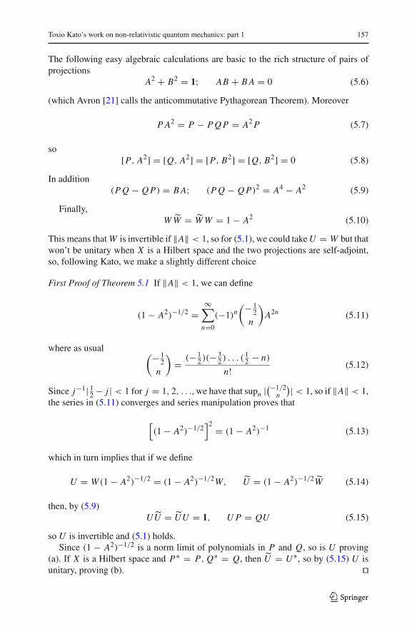
Tosio Kato’s work on non-relativistic quantum mechanics: part 1 157
The following easy algebraic calculations are basic to the rich structure of pairs ofprojections
A2 + B2 = 1; AB + B A = 0 (5.6)
(which Avron [21] calls the anticommutative Pythagorean Theorem). Moreover
P A2 = P − P Q P = A2P (5.7)
so[P, A2] = [Q, A2] = [P, B2] = [Q, B2] = 0 (5.8)
In addition(P Q − Q P) = B A; (P Q − Q P)2 = A4 − A2 (5.9)
Finally,W W = W W = 1 − A2 (5.10)
This means that W is invertible if ‖A‖ < 1, so for (5.1), we could takeU = W but thatwon’t be unitary when X is a Hilbert space and the two projections are self-adjoint,so, following Kato, we make a slightly different choice
First Proof of Theorem 5.1 If ‖A‖ < 1, we can define
(1 − A2)−1/2 =∞∑
n=0
(−1)n(− 1
2n
)A2n (5.11)
where as usual (− 12
n
)= (− 1
2 )(− 32 ) . . . ( 12 − n)
n! (5.12)
Since j−1| 12 − j | < 1 for j = 1, 2, . . ., we have that supn |(−1/2n
)| < 1, so if ‖A‖ < 1,the series in (5.11) converges and series manipulation proves that
[(1 − A2)−1/2
]2 = (1 − A2)−1 (5.13)
which in turn implies that if we define
U = W (1 − A2)−1/2 = (1 − A2)−1/2W, U = (1 − A2)−1/2W (5.14)
then, by (5.9)UU = UU = 1, U P = QU (5.15)
so U is invertible and (5.1) holds.Since (1 − A2)−1/2 is a norm limit of polynomials in P and Q, so is U proving
(a). If X is a Hilbert space and P∗ = P, Q∗ = Q, then U = U∗, so by (5.15) U isunitary, proving (b). ��
123

158 B. Simon
Theorem 5.1 for the self-adjoint Hilbert space case goes back to Sz-Nagy [454] whowas interested in the result because of its application to the convergent perturbationtheory of eigenvalues. His formula for U looks more involved than (5.2)/(5.14). Wolf[689] then extended the result to general Banach spaces but needed ‖P‖2‖P −Q‖ < 1and ‖1 − P‖2‖P − Q‖ < 1 which is a strictly stronger hypothesis.
In [320], Kato proved that if β �→ P(β) is a real analytic family of projections ona Banach space for β ∈ [0, B], then there exists a real analytic family of invertiblemaps, U (β) so that U (β)P(β)U (β)−1 = P(0). He did this using the same formalismhe had developed for his treatment of the adiabatic theorem (Kato [313] and Sect. 17in Part 2). In 1955, in an unpublished report [324], Kato presented all of the algebraabove (except for AB + B A = 0) and used it to prove Theorem 5.1 exactly as we doabove.
After Avron et al [31] found and exploited AB + B A = 0 (see below), Kato told methat he had found this relation about 1972 but didn’t have an application. Because [324]isn’t widely available, the standard reference for his approach to pairs of projections ishis book [345]. In [324], Kato noted that his expression was equal to the object foundby Sz-Nagy [454] but in the Banach space case, one could get better estimates fromhis formula for the object. In that note, he also remarked that when ‖P − Q‖ < 1,one can find a smooth, one parameter family of projections, P(t), 0 ≤ t ≤ 1 withP(0) = P and P(1) = Q so that the U obtained via his earlier method of solving adifferential equation was identical to the U of (5.2)/(5.14).
While this concludes Kato’s contribution to the subject of pairs of projections, Iwould be remiss if I didn’t say more about the rich structure of this simple setting,especially when ‖P − Q‖ ≥ 1 (in the self-adjoint Hilbert space setting one has that‖P − Q‖ ≤ 1 but for non-self-adjoint projections and the general case of Banachspaces, one often has ‖P − Q‖ > 1). There are two approaches. The one we’lldiscuss first is due to Avron–Seiler–Simon [31] and uses algebraic relations, especially(5.6). Since AB + B A = 0 is the signature of supersymmetry, we’ll call this thesupersymmetric approach. Here is a typical use of this method:
Theorem 5.2 (Avron et. al. [31]) Let P and Q be self-adjoint projections so thatP − Q is compact. For λ ∈ [−1, 1]\{0}, let Pλ be the projection onto the eigenspaceHλ ≡ {ϕ | Aϕ = λϕ}(a) If λ �= ±1, then
V = (1 − λ2)−1/2B � Hλ (5.16)
is a unitary map of Hλ onto H−λ.(b) For such λ, we have that
dimH−λ = dimHλ (5.17)
(c) If P − Q is trace class, thenTr(P − Q) ∈ Z (5.18)
(d) If ‖P − Q‖ < 1, then U ≡ sgn(B) is a unitary operator obeying (5.1). Indeed,
U PU−1 = Q, U QU−1 = P (5.19)
123

Tosio Kato’s work on non-relativistic quantum mechanics: part 1 159
Remarks 1. By sgn(B), we mean f (B) defined by the functional calculus [616,Section 5.1] where
f (x) =⎧⎨⎩
1, x > 0−1, x < 00, x = 0
This is unitary because ‖A‖ < 1 and B2 = 1− A2 implies that ker B = {0}. Onecan also write
U = B(1 − A2)−1/2 (5.20)
2. If we use (5.20) to define U in the general Banach space case when ‖P − Q‖ < 1,the same proof shows that we have (5.19). Indeed, since [A2, B] = 0, we havethat U 2 = 1 so (5.1) implies U QU−1 = P . So we get another proof of Theorem5.1 in the general Banach space case. However if P = Q, then B = 1 − 2P andA = 0 so by (5.20)
U = 1 − 2P (5.21)
Thus, U (P, P) �= 1 but see the remarks after Theorem 5.1.3. That Tr(P − Q) ∈ Z was first proven by Effros [134] and can also be proven
using the Krein spectral shift [616, Problem 5.9.1]. It is also true if P, Q arenot necessarily self-adjoint projections in a Hilbert space and for suitable Banachspace cases; see below.
Proof (a) If Aϕ = λϕ, then
ABϕ = −B Aϕ = −λBϕ (5.22)
so B maps Hλ toH−λ. Since
‖Bϕ‖2 = 〈ϕ, B2ϕ〉 = 〈ϕ, (1 − A2)ϕ〉 = (1 − λ2)‖ϕ‖2
we see that V is norm preserving.If ψ ∈ H−λ, then, by the above, ϕ ≡ (1 − λ2)−1Bψ ∈ Hλ and Bϕ = ψ so
ranB � Hλ is all of H−λ and thus V is unitary.(b) is immediate from (a)(c) Lidskii’s Theorem for self-adjoint operators says that if C is a self-adjoint trace
class operator, and for any λ �= 0, we define Hλ = {ϕ | Cϕ = λϕ}, then
Tr(C) =∑λ�=0
λ dim(Hλ) (5.23)
For the self-adjoint case this is easy since Tr(C) = ∑∞n=0〈ψn, Cψn〉 for any trace class
operator and any orthonormal basis (see [616, Theorem 3.6.7]) and any self-adjointcompact operator has an orthonormal basis of eigenvectors (see [616, Theorem 3.2.1]).By (b), the terms of (5.23) for λ and −λ when C = A cancel so long as λ �= ±1, so
Tr(A) = dimH1 − dimH−1 ∈ Z (5.24)
123

160 B. Simon
(d) Since ‖A‖ < 1, B2 = 1− A2 ≥ ε > 0 for ε = 1−‖A‖2. Thus, |B| is invertibleand
U = B|B|−1 (5.25)
is unitary since U = U∗ and U 2 = B2|B|−2 = 1.Moreover, since |B| commutes with A and B (since [B2, P] = [B2, Q] = 0) and
B anticommutes with A, we see that
U BU−1 = B, U AU−1 = −A (5.26)
SinceP = 1
2 (A − B + 1), Q = 12 (−A − B + 1) (5.27)
(5.26) implies (5.19). ��We can also say something about non-self-adjoint projections on Hilbert spaces
and also about the general Banach space case. The spectral theory of general compactoperators, A, is more subtle than the self-adjoint case ([616, Section 3.3]). One has thatσ(A)\{0} is discrete, a notion explained in Sect. 2. Thus, if we define for λ ∈ σ(A)\{0}
Pλ = 1
2π i
∮|z−λ|=δ
dz
z − A(5.28)
for δ < dist(λ, σ (A)\{λ}) and Hλ = ran Pλ, then dim(Hλ) < ∞ and is called thealgebraic multiplicity of λ. Also, as explained in Sect. 2,
APλ = λPλ + N (5.29)
where N is nilpotent, indeed N dim(Hλ) = 0 so
ϕ ∈ Hλ ⇒ (A − λ)dim(Hλ)ϕ = 0 (5.30)
Lidskii’s Theorem says that for trace class Hilbert space operators, (5.23) stillholds. Its proof [616, Section 3.12] is more subtle. Lidskii’s Theorem doesn’t hold onall Banach spaces (where there is an analog of the trace on a class known as nuclearoperators). We say that an operator, C on a Banach space, X , obeys Lidskii’s Theoremif C is nuclear and obeys (5.23)—see [151,484] for discussions on when this holds.
Theorem 5.3 Let P, Q be two projections on a Banach space, X, so that A = P − Qis compact. Then
(a) λ ∈ σ(A)\{1,−1} ⇒ −λ ∈ σ(A)
(b) For such λ, we have thatdimHλ = dimH−λ (5.31)
(c) If ±1 /∈ σ(A), then there exists an invertible map U so that (5.19) holds.(d) If A obeys Lidskii’s theorem, then Tr(P − Q) ∈ Z.
123

Tosio Kato’s work on non-relativistic quantum mechanics: part 1 161
Remark (d) was proven by Kalton [304] using different methods. The results (a)–(c)and the proof we give of (d) is new in the present paper.
Proof (a),(b) For any z ∈ C, we have that B(A−z) = −(A+z)B so, if z,−z /∈ σ(A),we see that
B(A − z)−1 = −(A + z)−1B (5.32)
Since σ(A)\{0} is a set of isolated points, for any λ �= 0, we can find ελ > 0 sothat σ(A)∩ {z | 0 < |z − λ| ≤ ελ} = ∅. Taking into account that z �→ −z reverses thedirection of a contour, by picking 0 < δ < min(ελ, ε−λ) in (5.28) and using (5.32),we see that
B Pλ = P−λ B (5.33)
where Pλ is defined by (5.28) with δ small even if λ /∈ σ(A) (in which case Pλ = 0).Suppose λ �= ±1. Since A leaves Hλ invariant and σ(A � Hλ) = {λ}, we have
that (1 − A2) = (1 − A)(1 + A) restricted toHλ has an inverse R. Thus RB is a leftinverse to B as a map of Hλ → H−λ so B as a map between those spaces is 1–1.This implies that dimHλ ≤ dimH−λ. By interchanging λ and −λ, we see that (5.31)holds which implies (a) and (b).
(c) SinceB B = B B, B A = −AB
(5.27) implies thatB P = Q B, B Q = P B (5.34)
We can take U = B if we show that B is invertible. Since ±1 /∈ σ(A), we see that(1 − A)−1(1 + A)−1B is a two sided inverse for B.
(d) From Lidskii’s theorem and (5.31), we see that (5.24) holds.
Our final result from the supersymmetric approach returns to the self-adjoint case.We define for projections P, Q:
KP,Q = ran P ∩ ker Q = {ϕ | Pϕ = ϕ, Qϕ = 0} (5.35)
Theorem 5.4 Let P, Q be two self-adjoint projections on a Hilbert space, H. Thenthere exists a unitary map, U, obeying (5.19) if and only if
dimKP,Q = dimK1−P,1−Q (5.36)
Moreover, if such a U exists, one can choose it so that
U = U∗, U 2 = 1 (5.37)
Remarks 1. In (5.36), both sides may be infinite.2. If ±1 are isolated points of the spectrum of A and are discrete eigenvalues, then
K : ran P → ranQ by K = Q P � ran P is a Fredholm operator [616, Section3.15], both sides of (5.36) are finite and their difference is the index of K . So, in thiscase, the theorem says that U obeying (5.19) exists if and only if index(K ) = 0.This special case is in [31].
123

162 B. Simon
3. The general case of this theorem is due to Wang, Du and Dou [694] whose proofused the Halmos representation discussed below. Our proof here is from Simon[617]. Two recent papers [70,124] classify all solutions of (5.19)
4. Operators obeying (5.37) are called symmetries by Halmos–Kakutani [217]
Proof IfU exists, it is easy to see thatU must be a unitary map ofKP,Q toK1−P,1−Q ,so (5.36) must hold.
For the converse, suppose that (5.36) holds. Clearly, P, Q leave both KP,Q andK1−P,1−Q invariant and soH1 = KP,Q ⊕K1−P,1−Q . LetH2 = H⊥
1 soH = H1⊕H2.Since (5.36) is assumed, there exists W : KP,Q → K1−P,1−Q unitary and onto. DefineonH1 as a direct sum
U1 =(
0 WW ∗ 0
)
Then U 21 = 1 and U∗
1 = U1 and for the restrictions of P, Q to H1, we have thatU1P1U−1
1 = Q1, U1Q1U−11 = P1.
So it suffices to prove the result for H2, i.e. in the special case that KP,Q =K1−P,1−Q = {0}. If that holds, we have that ker(1 − A2) = {0}, so ker(B) = {0}and U2 ≡ sgn(B) is unitary. Since U2A2 = −A2U2, U2B2 = B2U2, we get thatU2P2U−1
2 = Q2, U2Q2U−12 = P2 by (5.27). Clearly, also U 2
2 = 1, U∗2 = U2.
Our final big topic in this section concerns the Halmos representation. As a firststep, we note that
Proposition 5.5 Let P, Q be two orthogonal projections on a Hilbert space, H andlet A, B be given by (5.5). Then:
(a) KP,Q = {ϕ | Aϕ = ϕ}, K1−P,1−Q = {ϕ | Aϕ = −ϕ}(b) KP,1−Q = {ϕ | Bϕ = −ϕ}, K1−Q,P = {ϕ | Bϕ = ϕ}(c) KP,1−Q ⊕ K1−Q,P = {ϕ | Aϕ = 0}
KP,Q ⊕ K1−P,1−Q = {ϕ | Bϕ = 0}(d) These four spaces are mutually orthogonal.(e) All four spaces are {0} if and only if ker A = ker B = {0}.Proof (a) P ≤ 1, Q ≥ 0 so Aϕ = ϕ ⇒ ‖ϕ‖2 ≥ 〈ϕ, Pϕ〉 = ‖ϕ‖2 + 〈ϕ, Qϕ〉 ⇒
〈ϕ, Qϕ〉 = 0 ⇒ 〈Qϕ, Qϕ〉 = 0 ⇒ Qϕ = 0 ⇒ (since (P − Q)ϕ = ϕ) Pϕ =ϕ ⇒ ϕ ∈ KP,Q . Conversely, ϕ ∈ KP,Q ⇒ Pϕ = ϕ&Qϕ = 0 ⇒ Aϕ = ϕ. Theproof of the second statement is similar.
(b) Similar to (a) using B = (1 − P) − Q.(c) The two spaces in the first statement are orthonormal by (b) and the mutual
orthogonality of eigenspaces. Since A2ϕ = (1−B2)ϕ, that direct sum is ker A2 =ker A. Conversely, if Aϕ = 0, then (1 − B2)ϕ = A2ϕ = 0. If ϕ± = 1
2 (1∓B)ϕ,then ϕ± ∈ ker(1± B) and ϕ = ϕ+ + ϕ−, so by (b), ϕ ∈ KP,1−Q ⊕K1−Q,P . Thesecond relation has a similar proof.
(d) Immediate from the orthogonality of different eigenspaces of a self-adjoint oper-ator.
(e) Immediate from (c). ��
123

Tosio Kato’s work on non-relativistic quantum mechanics: part 1 163
We say that two orthogonal projections are in generic position if ker A = ker B ={0}, equivalently if KP,Q,K1−P,1−Q,KP,1−Q,K1−Q,P are all {0}. The Halmos twoprojection theorem says
Theorem 5.6 (Halmos Two Projection Theorem) Let P, Q be self-adjoint projectionson a Hilbert space,Hwhich are in generic position. LetB1 = ran P, B2 = ran(1−P).Then there exists a unitary map W from B1 onto B2 and self-adjoint operators C >
0, S > 0 on B1 withC2 + S2 = 1, [C, S] = 0 (5.38)
so that under H = B1 ⊕ B2,
P =(
1 00 0
)(5.39)
Q =(
C2 C SW −1
WC S W S2W −1
)(5.40)
Remarks 1. There are alternate ways that this theorem is often expressed. Rather thanstate it for pairs with generic position, the theorem says that the space is a direct sumof six spaces, two of the form just given and the other four simultaneous eigenspaceswith Aϕ = λϕ, Bϕ = κϕ with λ, κ ∈ {0, 1}. Sometimes, (5.40) is written:
Q =(
1 00 W
)(C2 C SC S S2
)(1 00 W
)−1
where the first factor maps B1 ⊕B1 to B1 ⊕B2 and the middle factor is an operator onB1 ⊕ B1. Some authors even implicitly use the first matrix above to identify H withB1 ⊕ B1 and only write the middle factor above.
2. C and S stand, of course, for cosine and sine. One often defines an operator, �with spectrum in [0, π/2] so that C = cos(�), S = sin(�). While 0 and/or 1 may liein the spectrum of �, they cannot be eigenvalues.
3. This result is due to Halmos [216]. There were earlier related results by Krein et.al. [391], Dixmier [120] and Davis [106]. The proof we give here is due to Amrein–Sinha [13].
Proof By the aboveker A = ker B = {0} (5.41)
Write the polar decompositions [616, Section 2.4]
A = UA|A|, B = UB |B| (5.42)
By (5.41), UA and UB are unitary and as functions of A and B respectively, theycommute with A and B respectively. It also holds that they each commute with both|A| and |B| (since, for example, |B| commutes with A and so |A| and so UA =s − lim A(|A| + ε)−1). Multiplying AB + B A by (|A| + ε)−1 and (|B| + ε)−1 andtaking ε to zero, we see that
123

164 B. Simon
UAUB = −UBUA ⇒ (UAUB)2 = −1 (5.43)
We’ve already seen that · �→ UA · U−1A interchanges P and Q. Since B is the A
when P is replaced by 1 − P , we see that · �→ UB · U−1B interchanges Q and 1 − P
and similarly, it interchanges 1 − Q and P .Let U = UAUB . Then we have that
U PU−1 = (1 − P), U (1 − P)U−1 = P
U QU−1 = (1 − Q), U (1 − Q)U−1 = Q (5.44)
which, in particular, implies thatU [B1] is all ofB2 (so they have the same dimension).Define W = U � B1 which we’ve just seen is a unitary map from B1 onto B2. In
the B1 ⊕ B2 decomposition, (5.39) is obvious. Moreover the decomposition of Q is
Q =(
P Q P � B1 P Q(1 − P) � B2(1 − P)Q P � B1 (1 − P)Q(1 − P) � B2
)(5.45)
By the formula for B, B P = −Q P , so P|B|2P = P B2P = P Q P . Similarly(1 − P)|A|2(1 − P) = (1 − P)Q(1 − P), P B A(1 − P) = P Q(1 − P) and (1 −P)AB P = (1 − P)Q P .
P|B|2P is already an operator on B1. Using [U, |A|2] = 0, we can write
(1 − P)|A|2(1 − P) = U PU−1|A|2U PU−1 = U P|A|2PU−1
Next note that U P|A|2U−1 � B2 = W (|A|2 � B1)W −1. If we define
C = |B| � B1, S = |A| � B1 (5.46)
then the above calculation and similar calculations on the off-diagonal piece implies(5.40).
Böttcher–Spitkovsky [69] is a review article on lots of applications of the Halmosrepresentation.Wemention also Lenard [421] who computes the joint numerical range(i.e. {(〈ϕ, Pϕ〉, 〈ϕ, Qϕ〉) | ‖ϕ‖ = 1}) for pairs of projections in terms of the operator� of remark 2 to Theorem 5.6. This range is a union of certain ellipses.
Finally, we mention one result that Kato proved in 1960 [332] that turns out to beconnected to pairs of self-adjoint projections, although Kato didn’t himself mentionor exploit this connection.
Theorem 5.7 Let � be a general (i.e. not necessarily self-adjoint) projection in aHilbert space, H. Suppose that � �= 0, 1. Then
‖�‖ = ‖1 − �‖ (5.47)
Kato has this as a Lemma in a technical appendix to [332], but it is now regarded asa significant enough result that Szyld [632] wrote an article to advertise it and explain
123

Tosio Kato’s work on non-relativistic quantum mechanics: part 1 165
myriad proofs ([69] also discusses proofs). Del Pasqua [111] and Ljance [433] foundproofs slightly before Kato but the methods are different and independent; indeed, formany years, no user of the result seemed to know of more than one of these threepapers.
Ljance’s proof [433] shows a close connection to pairs of projections. Let P be theorthogonal projection on ran(�) and Q the orthogonal projection onto ran(1 −�) (Pand Q must obey ker(P) ∩ ker(Q) = ker(1− P) ∩ ker(1− Q) = {0} and every suchpair of orthogonal projections corresponds to an oblique projection �). Then one canshow Ljance’s formula (see [69])
‖�‖ = 1
(1 − ‖P Q‖2)1/2 (5.48)
so that (5.47) follows from ‖Q P‖ = ‖(Q P)∗‖ = ‖P Q‖.Del Pasqua [111] noted that (5.47) might fail in general Banach spaces—indeed, it
is now known [211] that if (5.47) holds for all projections in a Banach space, X, thenits norm comes from an inner product.
6 Eigenvalue perturbation theory, V: Temple–Kato inequalities
While strictly speaking the central material in this section is not so much about per-turbation theory as variational methods, the subjects are related as Kato mentionedin several places, so we put it here. In fact, following Kato, we’ll see the inequali-ties proven here can be used to prove certain irregular perturbations yield asymptoticperturbation series. Kato also had several other papers about variational methods forscattering phase shifts [311,317,318] and for an aspect of Thomas–Fermi theory [267](not the energy variational principle central to TF theory but one concerning a techni-cal issue connected to the density at the nucleus). But none of these other papers hadthe impact of the work we discuss in this review, so we will not discuss them further.
Let A be a self-adjoint operator bounded from below and ‖ϕ‖ = 1 with ϕ ∈ D(A).Then Rayleigh’s principle says that
λ ≡ inf σ(A) ≤ 〈ϕ, Aϕ〉 ≡ ηϕ (6.1)
In 1928, Temple [637,638] proved a complementary lower bound in case
σ(A) ⊂ {λ} ∪ [μ,∞) (6.2)
with μ > λ and λ a simple eigenvalue. So long as
ηϕ < μ (6.3)
we have Temple’s inequality
λ ≥ ηϕ − ε2ϕ
μ − ηϕ
(6.4)
123

166 B. Simon
where εϕ ≥ 0 and
ε2ϕ ≡ ‖(A − ηϕ)ϕ‖2 = 〈ϕ, A2ϕ〉 − 〈ϕ, Aϕ〉2 (6.5)
Temple’s inequality had historical importance. Before the advent of modern com-puters, variational calculations were difficult and estimating their accuracy wasimportant. If μ∗ ≤ μ (i.e. if one had a possibly crude lower bound on the secondeigenvalue), then (6.2)/(6.4) ⇒ |λ − ηϕ | ≤ ε2ϕ(μ∗ − ηϕ)−1 so long as ηϕ < μ∗.One of the early success of perturbation theoretic quantum electrodynamics was thecalculation of the Lamb shift in Hydrogen. That was possible because the unshiftedHydrogen ground state was known precisely. To check the Lamb shift in Helium,one needed to know its ground state to very high order (the Lamb shift is about onehundred thousandth of that binding energy). The necessary calculations were done byKinoshita [371,372] and Pekeris [478–480] using variational calculations which inPekeris’ case involved 1078 parameter trial functions. They used Temple’s inequal-ity to estimate how accurately they had computed this ground state energy. In fact,Kinoshita sketched a proof of Temple’s inequality in his paper using Kato’s method(he quoted Kato’s paper). The result was the verification of the Lamb shift in Heliumto within experimental error.
In 1949, Kato [307] (with an announcement in Physical Review [312]) in one of hislittle gems found a simple proof of Temple’s inequality and also extended the resultto any eigenvalue. Here is his theorem:
Theorem 6.1 (Temple–Kato inequality) Let A be any self-adjoint operator and letϕ ∈ D(A). Let (α, ζ ) ⊂ R so that
α < ηϕ < ζ (6.6)
and so thatε2ϕ < (ηϕ − α)(ζ − ηϕ) (6.7)
Then:(a) σ(A) ∩ (α, ζ ) �= ∅
If σ(A) ∩ (α, ζ ) contains only a single point, λ, then
(b) ηϕ − ε2ϕ
ζ − ηϕ
≤ λ ≤ ηϕ + ε2ϕ
ηϕ − α(6.8)
If, in addition, λ is a simple eigenvalue with associated eigenvector, ψ , with ‖ψ‖ = 1and 〈ψ, ϕ〉 ≥ 0 and if εϕ < δ ≡ min(ηϕ − α, ζ − ηϕ), then
(c) ‖ϕ − ψ‖ ≤⎡⎣2 − 2
(1 − ε2ϕ
δ2
)1/2⎤⎦1/2
(6.9)
123

Tosio Kato’s work on non-relativistic quantum mechanics: part 1 167
Remarks 1. As we’ll see, a version of (6.8) holds even if we don’t suppose there isonly one point in σ(A) ∩ (α, ζ ), namely if
γ0 = ηϕ − ε2ϕ
ζ − ηϕ
; κ0 = ηϕ + ε2ϕ
ηϕ − α(6.10)
then σ(A) ∩ (α, κ0] �= ∅ and σ(A) ∩ [γ0, ζ ) �= ∅2. If we take α → −∞ and ζ = ηϕ +1, the upper bound in (6.8) is just the Rayleigh
bound (6.1) and if we take ζ = μ, then the lower bound in (6.8) is just Temple’sinequality (6.4).
3. If 0 < α < 1, then
2 − 2(1 − α2)1/2 =[
4 − 4(1 − α2)
2 + 2(1 − α2)1/2
]
≤ 4α2
4(1 − α2)1/2=[
α
(1 − α2)1/4
]2
so (6.9) implies that
‖ϕ − ψ‖ ≤ ε
δ
(1 − ε2
δ2
)−1/4
(6.11)
which is how Kato writes it in Kato [321] (see Knyazev [382] for refined versionsof these types of estimates).
The proof we’ll give follows Kato’s approach (see also Harrell [221]). The key tothis proof is what Temple [640] calls Kato’s Lemma:
Lemma 6.2 Let A be a self-adjoint operator and ϕ ∈ D(A) with ‖ϕ‖ = 1. Then
σ(A) ∩ (α, ζ ) = ∅ ⇒ 〈ϕ, (A − α)(A − ζ )ϕ〉 ≥ 0 (6.12)
Proof The spectral theorem (see [616, Chapter V and Section 7.2]) says that A is adirect sum of multiplications by x on L2(R\(α, ζ ), dμ(x)). Since (x −α)(x − ζ ) ≥ 0for x ∈ R\(α, ζ ), we see that (A − α)(A − ζ ) ≥ 0.
Remark While we use the Spectral Theorem (as Kato did), all we need is a spectralmapping theorem, i.e. if f (x) = (x − α)(x − ζ ), then σ( f (A)) = f [σ(A)] andthe fact that an operator with spectrum in [0,∞) is positive. The spectral mappingtheorem for polynomials holds for elements of any Banach algebra and the proof in[616, Theorem 2.2.6] extends to unbounded operators. That this lemma follows fromconsiderations of resolvents only was noted by Temple [640].
Taking contrapositives in (6.12), we get the following Corollary (if Lemmas areallowed to have Corollaries):
Corollary 6.3 Let A be a self-adjoint operator and ϕ ∈ D(A) with ‖ϕ‖ = 1. Then
〈ϕ, (A − α)(A − ζ )ϕ〉 < 0 ⇒ σ(A) ∩ (α, ζ ) �= ∅ (6.13)
123

168 B. Simon
The final preliminary of the proof is
Lemma 6.4 Suppose that A is self-adjoint and that λ ∈ R is an isolated simpleeigenvalue with Aψ = λψ and ‖ψ‖ = 1. If ϕ ∈ D(A) with ‖ϕ‖ = 1 and
εϕ < δ ≡ dist(ηϕ, σ (A)\{λ}) (6.14)
and if the phase of ψ is changed so that 〈ϕ,ψ〉 ≥ 0, then
‖ϕ − ψ‖2 ≤ 2 − 2
(1 − ε2ϕ
δ2
)1/2
(6.15)
Proof Let P be the projection onto multiples of ψ . Since (A − ηϕ)2 ≥ δ2 on theA-invariant subspace ran(1 − P) (by the spectral theorem as in the proof of Lemma6.2), we have that
ε2ϕ = ‖(A − ηϕ)ϕ‖2 ≥ δ2‖(1 − P)ϕ‖2 (6.16)
so‖(1 − P)ϕ‖2 ≤ ε2ϕ/δ2 < 1 (6.17)
by (6.14). Since ‖(1 − P)ϕ‖2 + ‖Pϕ‖2 = 1, we see that (if 〈ψ, ϕ〉 ≥ 0)
〈ψ, ϕ〉 = ‖Pϕ‖ ≥(1 − ε2ϕ
δ2
)1/2
(6.18)
Since ‖ψ − ϕ‖2 = 2 − 2〈ψ, ϕ〉, (6.15) is immediate.
Proof of Theorem 6.1 (a) We have that
〈ϕ, (A − α)(A − ζ )ϕ〉 = 〈ϕ, (A − ηϕ)2ϕ〉 + 〈ϕ,[η2ϕ + αζ − (α + ζ )A
]ϕ〉
= ε2ϕ − (ηϕ − α)(ζ − ηϕ) < 0 (6.19)
by (6.7). By Corollary 6.3, we see that σ(A) ∩ (α, ζ ) �= ∅.(b) As in the proof of (6.19), for any γ, κ , we have that
〈ϕ, (A − γ )(A − κ)ϕ〉 = ε2ϕ − (ηϕ − γ )(κ − ηϕ) (6.20)
Fix κ = ζ . Then, using ζ > ηϕ :
RHS of (6.20) < 0 ⇐⇒ γ < γ0 (6.21)
(with γ0 given by (6.10)) so by Corollary 6.3,
γ < γ0 ⇒ σ(A) ∩ (γ, ζ ) �= ∅ (6.22)
123

Tosio Kato’s work on non-relativistic quantum mechanics: part 1 169
Since σ(A) is closed, this implies that
σ(A) ∩ [γ0, ζ ) �= ∅ (6.23)
Similarly,σ(A) ∩ (α, κ0] �= ∅ (6.24)
In particular, if there is a single point, λ, in (α, ζ ), we must have that λ ∈ (α, κ0]∩[γ0, ζ ) = [γ0, κ0] which is (6.8).
(c) This is Lemma 6.4.��
Kato exploited what are now called the Temple–Kato inequalities in his thesis toprove results on asymptotic perturbation theory. Below are two typical results whoseproofs are very much in the spirit of this work of Kato—see Sect. 3 for what it meansfor an eigenvalue to be stable.
Theorem 6.5 Let A0 be a self-adjoint operator on a Hilbert space, H. Let B be asymmetric operator with D(A0)∩ D(B) ≡ D dense in H and a core for A0. For eachβ > 0 (perhaps only for sufficiently small such β), let A(β) be a self-adjoint extensionof A0 + βB � D. Let E0 be a simple, discrete eigenvalue for A0 which is stable forA(β). Let ϕ ∈ D(A0), ‖ϕ‖ = 1 and A0ϕ = E0ϕ. Suppose that ϕ ∈ D(B). Then theeigenvalue, E(β) of A(β) near E0 obeys
E(β) = E0 + β〈ϕ, Bϕ〉 + O(β2) (6.25)
Proof SinceD is a core and for η ∈ D, z ∈ C\R, [(A(β)− z)−1 − (A0 − z)−1](A0 −z)η = −β(A(β)−z)−1Bηwe see that A(β) → A0 in strong resolvent sense as β ↓ 0.By the definition of stability, there is an interval (α, ζ ) containing E0, so that for smallβ, A(β) has a unique eigenvalue, E(β), in (α, ζ ). Showing the operator involved in asuperscript, we see that
ηA(β)ϕ = E0 + β〈ϕ, Bϕ〉 → E0
Since (A(β) − ηA(β)ϕ )ϕ = β(B − 〈ϕ, Bϕ〉)ϕ, we see that(εA(β)ϕ
)2 = β2(‖Bϕ‖ − 〈ϕ, Bϕ〉2) = O(β2)
so, by the Temple–Kato inequalities, E(β) − ηA(β)ϕ = O(β2) which is (6.25)
To go to the next order, we need the reduced resolvent, S, of A0 at E0, definedin Sect. 2 (see (2.8)). In his thesis, Kato realized that contour integrals of B(A0 −z)−1 . . . B(A0 − z)−1ϕ could be expressed in terms of S. In particular, the first orderformal eigenvector for A(β) is
ψ1(β) = ϕ − βSBϕ (6.26)
123

170 B. Simon
Since ranS ⊂ ran(1 − P) is orthogonal to ϕ, we see that
‖ψ1(β)‖2 = 1 + β2‖SBϕ‖2 (6.27)
For ψ1(β) to be in D(B), we will need to suppose that
ϕ ∈ D(B), SBϕ ∈ D(B) (6.28)
We can also write down the first three perturbation coefficients for the energy (see forexample [497, pg 7]):
E1 = 〈ϕ, Bϕ〉, E2 = −〈Bϕ, SBϕ〉 (6.29)
E3 = E1E2 + 〈Bϕ, SBSBϕ〉 (6.30)
Straightforward calculations show that
(A0 − E0)ψ1(β) = −β(1 − P)Bϕ
(A(β) − E0)ψ1(β) = βE1ϕ − β2BSBϕ
since β P Bϕ = βE1ϕ. Thus:
(A(β) − E0 − βE1)ψ1(β) = β2E1SBϕ − β2BSBϕ
From this, using (6.27), one sees easily that
〈ψ1(β), A(β)ψ1(β)〉 = (E0 + βE1 + β2E2 + β3E3)‖ψ1(β)‖2 + O(β4)(6.31)
‖[
A(β) − (E0 + βE1 + β2E2 + β3E3)]ψ1(β)‖2 = O(β4) (6.32)
Thus, we have, using ψ1(β)/‖ψ1(β)‖ as a trial vector
Theorem 6.6 Under the hypotheses of Theorem 6.5 if also (6.28) holds, then
E(β) = E0 + βE1 + β2E2 + β3E3 + O(β4) (6.33)
‖ϕ(β) − ψ1(β)‖ = O(β2) (6.34)
where ϕ(β) is the normalized eigenvector for A(β) chosen so that for small β,〈ϕ(β), ϕ〉 > 0.
As Kato noted in his thesis, this idea shows if all the terms for the nth order formalseries for the eigenvector lie inH, then one gets asymptotic series for the energy witherrors of order O(β2n), i.e. the 2n coefficients E0, . . . , E2n−1 but the method doesn’thandle odd powers. Indeed in [316], he said: “However, there has been a serious gapin the series of these conditions; for all of them had in common the property that theygive the expansion of the eigenvalues up to even orders of approximation, and therewas no corresponding theorem giving an expansion up to an odd order.” Personally,
123

Tosio Kato’s work on non-relativistic quantum mechanics: part 1 171
I think “serious” is a bit strong given that he handles the case of infinite order (for methe most important) and first order results but it shows he was frustrated by a problemhe tried to solve without initial success. But in [309], he put in a Note Added in Proofannouncing he had solved the problem! The solution appeared in [322]. For example,if A0 ≥ 0, B ≥ 0, he proved that if ϕ ∈ Q(B), then E(β) = E0 + E1β + o(β) and ifB1/2ϕ ∈ Q(B1/2A−1
0 B1/2), he proved that E(β) = E0 + E1β + E2β2 + o(β2). Not
surprisingly, in addition to estimates of Temple–Kato type, the proofs use a variant ofquadratic form methods. I note that Kato did not put any of these results in his bookwhere his discussion of asymptotic series applies to general Banach space settings andnot just positive operators and the ideas are closer to what we put in Sect. 3.
Besides the original short paper on Temple–Kato inequalities, Kato returned to thesubject several times. In two papers [321,357], he considered the fact that in someapplications of interest, the natural trial vector hasϕ ∈ Q(A), not D(A). Trial functionsonly in Q(A) are fine for the Rayleigh upper bound but if ϕ /∈ D(A), then εA
ϕ = ∞, soϕ cannot be used for Temple’s inequality or the Temple–Kato inequality. Of course,one could look at the Temple–Kato inequality for
√A if A ≥ 0 but calculation of
〈ϕ,√
Aϕ〉 may not be easy for, say, a second order differential operator where√
Ais a pseudo-differential operator. But such operators can often be written A = T ∗Twhere T is a first order differential operator. Variants of the Temple–Kato inequalityfor operators of this form are the subject of two papers of Kato [321,357]. Kato et al.[359] studies an application of these ideas.
Interesting enough, while Kato’s work was 20 years after Temple, Temple wasyoungwhen he did that work andwas still active in 1949 and he reacted toKato’s paperwith two of his own [639,640]. George Frederick James Temple (1901–1992) was amathematician with a keen interest in physics—he wrote two early books on quantummechanics in 1931 and 1934. He spent much of his career at King’s College, Londonalthough for the last fifteen years of it, he held the prestigious Sedleian Chair of NaturalPhilosophy at Oxford, the chair going back to 1621. He was best known in Britishcircles for a way of discussing distributions as equivalence classes of approximatingsmooth functions, an idea that was popular because the old guard didn’t want to thinkabout the theory of topological vector spaces central to Schwartz’ earlier approach.His other honors include a knighthood (CBE, for War work), a fellowship in andthe Sylvester Medal of the Royal Society. At age 82, he became a benedictine monkand spent the last years of his life in a monastery on the Isle of Wright. The longbiographical note of his life written for the Royal Society [370] doesn’t even mentionTemple’s inequality!
Davis [105] extended what he calls “the ingenious method of Kato” by replacingthe single interval (α, ζ ) by a finite union of intervals. Thirring [643] has discussedTemple’s inequality as a consequence of the Feshbach [149,150] projection method(which mathematicians call the method of Schur [545] complements). Turner [658]andHarrell [221] have extensions to the casewhere A is normal rather than self-adjointand Kuroda [400] to n commuting self-adjoint operators (and so including the normalcase). Cape et al. [81] apply Temple–Kato inequalities to graph Laplacians. Golub–van der Vost [195] have a long review on eigenvalue values bounds mentioning thatby the time of their review in 2000, Temple–Kato inequalities had become a standardpart of linear algebra.
123

172 B. Simon
7 Self-adjointness, I: Kato’s theorem
This is the first of four sections on self-adjointness issues.We assume the reader knowsthe basic notions, including what an operator closure and an operator core are and themeaning of essential self-adjointness. A reference for these things is [616, Section7.1].
This section concerns the Kato–Rellich theorem and its application to provethe essential self-adjointness of atomic and molecular Hamiltonians. The quantummechanical Hamiltonians typically treated by this method are bounded from below.Section 8 discusses cases where V (x) ≥ −cx2 − d like Stark Hamiltonians. Sec-tion 9 discusses Kato’s contribution to the realization that the positive part of V can bemore singular than the negative part without destroying essential self-adjointness andSect. 10 turns to Kato’s contribution to the theory of quadratic forms. To save ink, inthis article, I’ll use “esa” as an abbreviation for “essentially self-adjoint” or “essentialself-adjointness” and “esa-ν” for “essentially self-joint on C∞
0 (Rν).”.As we’ve mentioned, Kato’s 1951 paper [314] is a pathbreaking contribution of
great significance. He considered N -body Hamiltonians on L2(RνN ) of the formalform
H = −N∑
j=1
1
2m j� j +
∑i< j
Vi j (xi − x j ) (7.1)
where x ∈ RνN is written x = (x1, . . . , xN ) with x j ∈ R
ν , � j is the ν-dimensionalLaplacian in x j and each Vi j is a real valued function on R
ν . In 1951, Kato consideredonly the physically relevant case ν = 3.
If there are N+k particles in the limitwhere themasses of particles N+1, . . . , N+kare infinite, one considers an operator like H but adds terms
N∑j=1
Vj (x j ), Vj (x) =N+k∑
�=N+1
Vj�(x − x�) (7.2)
where xN+1, . . . , xN+k are fixed points in Rν .
More generally, one wants to consider (as Kato did) Hamiltonians with the centerof mass removed. We discuss the kinematics of such removal in Sect. 11 in Part 2. Wenote that the self-adjointness results on the Hamiltonians of the form (7.1) easily implyresults on Hamiltonians (on L2(R(N−1)ν)) with the center of mass motion removed.Of especial interest is the Hamiltonian of the form (7.2) with N = 1, i.e.
H = −� + W (x) (7.3)
on L2(Rν)which we’ll call reduced two body Hamiltonians (since, except for a factorof (2μ)−1 in front of −�, it is the two body Hamiltonian with the center of massremoved).
Kato’s big 1951 result was
123

Tosio Kato’s work on non-relativistic quantum mechanics: part 1 173
Theorem 7.1 (Kato’sTheorem [314], First Form)Let ν = 3. Let each Vi j in (7.1) lie inL2(R3)+ L∞(R3). Then the Hamiltonian of (7.1) is self-adjoint on D(H) = D(−�)
and esa-(3N ).
Remarks 1. The same results holds with the terms in (7.2) added so long as each Vj
lies in L2(R3) + L∞(R3).2. Kato also notes the exact description of D(−�) on L2(Rν) in terms of the Fourier
transform (see [612, Chapter 6]) ϕ(k) = (2π)−ν/2∫
e−ik·xϕ(x)dνx :
D(−�) = {ϕ ∈ L2(Rν) |∫
(1 + k2)2|ϕ(k)|2dνk < ∞} (7.4)
3. The proof shows that the graph norms of H and −� on D(−�) are equivalent,so any operator core for −� is a core for H . Since it is easy to see that C∞
0 (R3N )
is a core for −�, the esa result follows from the self-adjointness claim, so weconcentrate on the latter.
4. Kato didn’t assume that V ∈ L2(R3)+ L∞(R3) but rather the stronger hypothesisthat for some R < ∞, one has that
∫|x |<R |V (x)|2d3x < ∞ and sup|x |≥R |V (x)| <
∞, but his proof extends to L2(R3) + L∞(R3).
5. Kato didn’t state thatC∞0 (R3N ) is a core but rather thatψ’s of the form P(x)e− 1
2 x2
with P a polynomial in the coordinates of x is a core (He included the 12 so the set
was invariant under Fourier transform.) His result is now usually stated in termsof C∞
0 .
If v(x) = 1/|x | on R3, then v ∈ L2(R3) + L∞(R3), so Theorem 7.1 has the
important Corollary, which includes the Hamiltonians of atoms and molecules:
Theorem 7.2 (Kato’s Theorem [314], Second Form) The Hamiltonian, H, of (7.1)with ν = 3 and each
Vi j (x) = zi j
|x | (7.5)
and this Hamiltonian with terms of the form (7.2) where
Vj (x) =N+k∑
�=N+1
z j�
|x − x�| (7.6)
are self-adjoint on D(−�) and esa-3N
Remark This result assures that the time dependent Schrödinger equation ψt =−i Hψt has solutions (since self-adjointness means that e−i t H exists as a unitaryoperator). The analogous problem for Coulomb Newton’s equation (i.e. solvabilityfor a.e. initial condition) is open for N ≥ 5!
As Kato remarks in [1], “the proof turned out to be rather easy”. It has three steps:
(1) The Kato–Rellich theorem which reduces the proof to showing that each Vi j isrelatively bounded for Laplacian on R
3 with relative bound 0.
123

174 B. Simon
(2) A proof that any function in L2(R3) + L∞(R3), as an operator on L2(R3), is−�-bounded with relative bound 0. This relies on a simple Sobolev estimate.
(3) A piece of simple kinematics that says that the two body estimate in step 2 extendsto one for vi j (xi − x j ) as an operator on L2(R3N ).
Step 1. The needed result (recall that A-bounded is defined in (2.14)):
Theorem 7.3 (Kato–Rellich Theorem) Let A be self-adjoint, B symmetric and let Bbe A-bounded with relative bound a < 1, i.e. D(A) ⊂ D(B) and for some fixed b andall ϕ ∈ D(A)
‖Bϕ‖ ≤ a‖Aϕ‖ + b‖ϕ‖ (7.7)
Then A + B is self-adjoint on D(A) and any operator core for A is one for A + B.
Remarks 1. This result is due to Rellich [504–508, Part III]. Kato found it in 1944,when he was unaware of Rellich’s work, so it is independently his.
2. The proof uses von Neumann’s criteria: a closed symmetric operator, C , on D(C)
is self-adjoint if and only if for some κ ∈ (0,∞), one has that ran(C ± iκ) =H. For C closed implies that ran(C ± iκ) are closed subspaces with ran(C ±iκ)⊥ = ker(C∗∓iκ). Thus, if C is self-adjoint, then ker(C∗∓iκ) = {0} provingone direction. For the other direction, suppose that ran(C ± iκ) = H. Given ψ ∈D(C∗), find ϕ ∈ D(C) with (C + iκ)ϕ = (C∗ + iκ)ψ (since ran(C + iκ) = H).Thus (C∗ + iκ)(ϕ − ψ) = 0. Since ran(C − iκ) = H = ker(C∗ + iκ)⊥, we havethat ϕ − ψ = 0. Thus D(C∗) = D(C) and C is self-adjoint.
3. For the rest of the proof, use ‖(C + iκ)ϕ‖2 = ‖Cϕ‖2 + |κ|2‖ϕ‖2 to see that
‖C(C ± iκ)−1‖ ≤ 1, ‖(C ± iκ)−1‖ ≤ |κ|−1 (7.8)
It follows from this (with C = A) that when (7.7) holds, one has that
‖B(A ± iκ)−1‖ ≤ a + b|κ|−1 (7.9)
Since a < 1, we can be sure that if |κ| is very large, then ‖B(A ± iκ)−1‖ < 1so using a geometric series, we have that 1 + B(A ± iκ)−1 is invertible whichimplies that it maps H onto H. Since (A ± iκ) maps D(A) onto H, we see that
(A + B ± iκ) = (1 + B(A ± iκ)−1)(A ± iκ) (7.10)
maps D(A) onto H. Thus by von Neumann’s criterion, A + B is self-adjoint onD(A). By a simple argument, ‖A·‖+‖·‖ is an equivalent norm to ‖(A+ B)·‖+‖·‖which proves the esa result.
4. The case B = −A shows that one can’t conclude self-adjointness of A + B onD(A) if (7.7) holds with a = 1 but Kato [345] proved that A + B is esa on D(A)
in that case and Wüst [690] proved the stronger result of esa on D(A) if one hasfor all ϕ ∈ D(A)
‖Bϕ‖2 ≤ ‖Aϕ‖2 + b‖ϕ‖2 (7.11)
123

Tosio Kato’s work on non-relativistic quantum mechanics: part 1 175
5. In some of my early papers, I called B Kato small if B was A − bounded withrelative bound less than 1 and Kato tiny if the relative bound was 0. I am pleasedto say that while many of my names (hypercontractive, almost Mathieu, Berry’sphase, Kato class,…) have stuck, this one has not!
Step 2. Kato began by considering ϕ ∈ L2(R3) with ϕ ∈ D(−�), i.e.∫(1 +
k2)2|ϕ(k)|2d3k < ∞. He noted that this implied that
∫|ϕ(k)|d3k =
∫(1 + k2)−1(1 + k2)|ϕ(k)|d3k
≤ ‖(1 + k2)−1‖2‖(1 − �)ϕ‖2 (7.12)
by the Schwarz inequality and Plancherel theorem. Thus
‖ϕ‖∞ ≤ (2π)−3/2∫
|ϕ(k)|d3k (7.13)
≤ C (‖�ϕ‖2 + ‖ϕ‖2) (7.14)
It follows that if V = V1 + V2 with V1 ∈ L2(R3), V2 ∈ L∞(R3), then as operatorson L2(R3)
‖V ϕ‖2 ≤ ‖V1ϕ‖2 + ‖V2ϕ‖2≤ ‖V1‖2‖ϕ‖∞ + ‖V2‖∞‖ϕ‖2≤ C‖V1‖2‖�ϕ‖2 + (C‖V1‖2 + ‖V2‖∞) ‖ϕ‖2 (7.15)
If f ∈ L2 and
f (n)(x) ={
f (x), if | f (x)| > n0, if | f (x)| ≤ n
(7.16)
then ‖ f (n)‖2 → 0 as n → ∞ by the dominated convergence theorem and for alln, ‖ f − f (n)‖∞ < ∞. It follows from (7.15) that any V ∈ L2(R3) + L∞(R3) is−�-bounded with relative bound zero as operators on L2(R3).
Step 3. In modern language, one shows that ifH = H1 ⊗H2 (tensor products aredefined, for example, in [612, Section 3.8]) and (7.7) holds, then
‖(B ⊗ 1)ϕ‖ ≤ a‖(A ⊗ 1)ϕ‖ + b‖ϕ‖ (7.17)
Thus, if V is a function of x1 alone, V (x1, . . . , xN ) = v(x1), v ∈ L2(R3) + L∞(R3)
so that (7.7) holds for v on L2(R3), then it also holds for B = V (x) and A = −�1 onL2(R3N ). Since |k1|2 ≤ |k|2, we conclude that V is −�-bounded with relative boundzero on L2(R3N ). By a coordinate change, the same is true for v(xi − x j ).
Rather than talk about tensor products, Kato used iterated Fourier transforms andstates inequalities like
supx1
[∫|ϕ(x1, . . . , xN )|2d3x2 . . . d3xN
]≤ C
∫(1 + k21)
2|ϕ(k)|2d3N k (7.18)
123

176 B. Simon
which is equivalent to the tensor product results. This concludes our sketch of Kato’sproof of his great theorem.
Kato states in the paper that he had found the results by 1944. Kato originallysubmitted the paper to Physical Review. Physical Review transferred the manuscriptto the Transactions of the AMSwhere it eventually appeared. They had trouble findinga referee and in the process the manuscript was lost (a serious problem in pre-Xeroxdays!). Eventually, von Neumann got involved and helped get the paper accepted. I’vealways thought that given how important he knew the paper was, von Neumann shouldhave suggested Annals ofMathematics and used his influence to get it published there.The receipt date ofOctober 15, 1948on the version published in theTransactions showsa long lag compared to the other papers in the same issue of the Transactions whichhave receipt dates of Dec., 1949 through June, 1950. Recently after Kato’s widowdied and left his papers to some mathematicians (see the end of Sect. 1) and somefascinating correspondence of Kato with Kemble and von Neumann came to light.There are plans to publish an edited version [181].
It is a puzzle why it took so long for this theorem to be found. One factor may havebeen von Neumann’s attitude. Bargmann told me of a conversation several youngmathematicians had with von Neumann around 1948 in which von Neumann toldthem that self-adjointness for atomic Hamiltonians was an impossibly hard problemand that even for the Hydrogen atom, the problemwas difficult and open. This is a littlestrange since, using spherical symmetry, Hydrogen can be reduced to a direct sum ofone dimensional problems. For such ODEs, there is a powerful limit point–limit circlemethod named after Weyl and Titchmarsh (although it was Stone, in his 1932 book,who first made it explicit). Using this, it is easy to see (there is one subtlety for � = 0since the operator is limit circle at 0) that the Hydrogen Hamiltonian is self-adjointand this appears at least as early as Rellich [509]. Of course, this method doesn’t workfor multielectron atoms. In any event, it is possible that von Neumann’s attitude mayhave discouraged some from working on the problem.
Still it is surprising that neither Friedrichs nor Rellich found this result. In exploringthis, it is worth noting that there is an alternate to step 2:
Step 2′. On R3, there is the well known operator inequality (discussed further in
Sect. 10 and in [615, Section 6.2]) known as Hardy’s inequality (A ≤ B for posi-tive operators is discussed in Sect. 10 and [616, Section 7.5]; for this case, it means〈ϕ, Aϕ〉 ≤ 〈ϕ, Bϕ〉 for all ϕ ∈ C∞
0 (R3)):
1
4r2≤ −� (7.19)
Since x ≤ εx2 + 14ε
−1 for x ∈ (0,∞), the spectral theorem implies that for anypositive, self-adjoint operator, C , we have that
C ≤ εC2 + 14ε
−1 (7.20)
so using this for C = −�, (7.19) implies that
1
4r2≤ ε(−�)2 + 1
4ε−1 (7.21)
123

Tosio Kato’s work on non-relativistic quantum mechanics: part 1 177
equivalently, for ϕ ∈ C∞0 (R3)
‖r−1ϕ‖2 ≤ 4ε‖−�ϕ‖2 + ε−1‖ϕ‖2 (7.22)
which implies that r−1 is −�-bounded with relative bound zero.Rellich used Hardy’s inequality in his perturbation theory papers [504–508] in a
closely related context. Namely he used (7.19) and (7.20) for C = r−1 to show thatr−1 ≤ 4ε(−�) + 1
4ε−1 to note the semiboundedness of the Hydrogen Hamiltonian.
Since Rellich certainly knew the Kato–Rellich theorem, it appears that he knew steps1 and 2′.
In a sense, it is pointless to speculate why Rellich didn’t find Theorem 7.2, but it isdifficult to resist. It is possible that he never considered the problem of esa of atomicHamiltonians, settling for a presumption that using the Friedrichs extension suffices(as Kato suggests in [1]) but I think that unlikely. It is possible that he thought aboutthe problem but dismissed it as too difficult and never thought hard about it. Perhapsthe most likely explanation involves Step 3: once you understand it, it is trivial, butuntil you conceive that it might be true, it might elude you.
Kato’s original paper required that the L2 piece have compact support (in therelevant variables). While it is easy to accommodate global L2, it is true that it isenough to be uniformly locally L2, i.e.
supx
∫|x−y|≤1
|V (y)|2d3y (7.23)
denoted L2uni f (R
3). It was Stummel [631] who first realized this. There are generallocalization techniques, originally developed for form estimates by Ismagilov [273],Morgan [447] and Sigal [554] (and discussed as the IMS localization formula in [101,Section 3.1]) which have operator versions. For a recent paper on these techniques,see Gesztesy et. al. [189]. For example, [616, Problem 7.1.9] proves:
Theorem 7.4 For each α ∈ Zν , let �α be the cube of side 3 centered at α and χα
its characteristic function. Let V be a measurable function on Rν so that for some
positive a, b and all α and all ϕ ∈ C∞0 (Rν)
‖V χαϕ‖2 ≤ a‖−�ϕ‖2 + b‖ϕ‖2 (7.24)
Then for any ε > 0, there is a bε so that for all ϕ ∈ C∞0 (Rν), we have that
‖V ϕ‖2 ≤ (a + ε)‖−�ϕ‖ + bε‖ϕ‖2 (7.25)
In particular, any V ∈ L2uni f (R
3) is −�-bounded on L2(R3) with relative bound 0.
In exploring extensions of Theorem 7.1, it is very useful to have simple self-adjointness criteria for − d2
dx2+ q(x) on L2(0,∞) which then translate to criteria for
−�+ V (x) if V (x) = q(|x |) is a spherically symmetric potential. If q ∈ L2loc(0,∞),
for each z ∈ C, the set of solutions of −u′′ + qu = zu (in the sense that u is C1, u′ is
123

178 B. Simon
absolutely continuous and u′′ is its L1loc derivative) is two dimensional. If all solutions
are L2 at ∞ (resp. 0), we say that − d2
dx2+ q(x) is limit circle at ∞ (resp. 0). If it is
not limit circle, we say it is limit point. It is a theorem that whether one is limit pointor limit circle is independent of z. However, in the limit point case, whether the set ofL2 solutions near infinity is 0 or 1 dimensional can be z dependent. One has the basic
Theorem 7.5 (Weyl limit point–limit circle theorem) Let q ∈ L2loc(0,∞). Then
− d2
dx2+ q(x) is esa on C∞
0 (0,∞) if and only if − d2
dx2+ q(x) is limit point at both 0
and ∞.
Remarks 1. This result holds for any interval (a, b) ⊂ R where a can be −∞ and/orb can be ∞.
2. If it is limit point at only one of 0 and ∞ and limit circle at the other point, thedeficiency indices (see [616, Section 7.1] for definitions) are (1, 1) and if it is limitcircle at both 0 and ∞, they are (2, 2). In particular if it is limit point at ∞ and∫ 10 |V (x)|dx < ∞, then the deficiency indices are (1,1) and the extensions aredescribed by boundary conditions cos θ u′(0) + sin θ u(0) = 0.
3. The ideas behind much of the theorem go back to Weyl [677,678,680] in 1910and predate the notion of self-adjointness. It was Stone [630] who first realized theimplications for self-adjointness and proved Theorem 7.5. [616, Thm 7.4.12] has asuccinct proof. Titchmarsh [653] reworked the theory so much that it is sometimescalled Weyl–Titchmarsh theory. For additional literature, see [94,131,423].
Example 7.6 (x−2 on (0,∞)) Let q(x) = βx−2. Trying xα in−u′′ +βx−2u = 0, onefinds that α(α − 1) = β is solved by α± = 1
2 (1± √1 + 4β). For β �= − 1
4 , this yieldstwo linearly independent solutions, so a basis. The larger solution (and sometimesboth) is not L2 at infinity, so it is always limit point there.
Forα ≥ − 14 , there is a positive solutionwhich implies that Hβ ≡ − d2
dx2+βx−2 ≥ 0.
If α < − 14 , the solutions oscillate and the real solutions have infinitely many zeros
which implies that the operator is not positive (see [616, Section 7.4]). Thus
− d2
dx2+ βx−2 ≥ 0 on C∞
0 (0,∞) ⇐⇒ β ≥ − 14 (7.26)
This is Hardy’s inequality on L2(0,∞).xα /∈ L2(0, 1) ⇐⇒ α ≤ − 1
2 . At β = 34 , α− = − 1
2 . Thus Hβ is always limitpoint at ∞ and is limit point at 0 if and only if β ≥ 3
4 , i.e.
− d2
dx2+ βx−2 is esa on C∞
0 (0,∞) ⇐⇒ β ≥ 34 (7.27)
A comparison theorem shows that if
q(x) ≥ 34 x−2 − c (7.28)
for some real c, then − d2
dx2+ q(x) is esa on C∞
0 (0,∞).
123

Tosio Kato’s work on non-relativistic quantum mechanics: part 1 179
On Rν , one defines spherical harmonics (see [615, Section 3.5]), {Y�m}D(ν,�)
m=1;�=0,1,...
on Sν−1, the unit sphere in Rν , to be the restriction to the unit sphere of harmonic
polynomials of degree �. These polynomials are a vector space of dimension D(ν, �) =�+ν−2ν−2
(ν−3+�ν−3
)and Y�m are a convenient orthonormal basis. Any function f ∈ S(Rν)
can be expanded in the form (r ∈ (0,∞), ω ∈ Sν−1)
f (rω) =∑�,m
r−(ν−1)/2 f�m(r)Y�m(ω) (7.29)
(where for ν ≥ 2, f�m vanishes so rapidly at r = 0 that r−(ν−1)/2 f�m(r) has a limitas r ↓ 0 which must be zero unless (�m) = (01)). Moreover, if σν is the area of theunit sphere, then
‖ f ‖2L2(Rν ,dν x)= σν
∑�,m
‖ f�m‖2L2(R,dr)(7.30)
and
(� f )�m =[
d2
dr2− (ν − 1)(ν − 3)
4r2− �(� + ν − 2)
r2
]f�m (7.31)
If V (r) = q(r), then −� + V is a direct sum of operators of the form
H�m(V ) = − d2
dr2+ q�(r) (7.32)
q�(x) = (ν − 1)(ν − 3)
4x2+ �(� + ν − 2)
x2+ q(x) (7.33)
It is easy to see that such direct sums are bounded frombelow (resp. esa) onC∞00 (R
ν) ≡C∞0 (Rν\{0}) if and only if each H�m is bounded from below (resp. esa) on C∞
0 (0,∞)
We conclude that
Proposition 7.7 On Rν , H (ν)
β ≡ −� + β|x |−2 on C∞00 (R
ν) is
(1) Bounded from below
H (ν)β ≥ 0 ⇐⇒ β ≥ − (ν − 2)2
4(7.34)
(2) H (ν)β is esa on C∞
00 (Rν) if and only if
β ≥ −ν(ν − 4)
4(7.35)
Remarks 1. This uses− (ν−1)(ν−3)4 − 1
4 = − (ν−2)2
4 and− (ν−1)(ν−3)4 + 3
4 = − ν(ν−4)4 .
2. (7.34) is the ν-dimensional Hardy inequality with optimal constant (see Sect. 10below).
123

180 B. Simon
3. By (7.28), if ν ≥ 4 and V is spherically symmetric and obeys V (x) ≥ − ν(ν−4)4|x |2 ,
then −� + V is esa-ν (discussed further in Sect. 9).4. In particular, C∞
00 (Rν) is an operator core for −� if and only if ν ≥ 4 and a form
core for −� if and only if ν ≥ 2.5. By (7.28), if γ > 2, then −� + λ|x |−γ (λ > 0) is esa on C∞
00 (Rν). If ν ≥ 5
and 2 < γ < ν/2, we have that |x |−γ ∈ L2(Rν) + L∞(Rν), so one can defineT ≡ −�+λ|x |−γ on C∞
0 (Rν) and it is easy to see that T is symmetric. It followsby general principles [616, Section 7.1] that T is esa-ν.
6. There is an intuition to explain why one loses self-adjointness of −� − |x |−γ
when γ > 2. If γ < 2, in classical mechanics there is an �2
|x |2 barrier which
dominates the −|x |−γ , so for almost every initial condition, the classical particleavoids the singularity at the origin. But when γ > 2, every negative energy initialcondition will fall into the origin in finite time so in classical mechanics, one needsto supplement with a rule about what happens when the particle is captured by thesingularity. The quantum analog is the loss of esa. There is of course a differenceat γ = 2 where classically there is a problem no matter the coupling but not inquantum mechanics. This is associated with the uncertainty principle. In the nextsection, we’ll see that this intuition is also useful to understand what happens withV ’s going to −∞ at spatial infinity.
We summarize in
Example 7.8 (|x |−2 in Rν ; ν ≥ 5) Rellich’s Inequality [510] (see also [616, Problem
7.4.10], Sect. 10 below, Gesztesy–Littlejohn [188] or Robinson [519] for a proof ofRellich’s inequality via a double commutator estimate like the one before (3.33) andHardy’s inequality; this proof is a variant of one of Schmincke [539]) says that onR
ν, ν ≥ 5, one hasν(ν − 4)
4‖|x |−2ϕ‖ ≤ ‖�ϕ‖ (7.36)
for any ϕ ∈ C∞0 (Rν). (Of course, this also hold if ν ≤ 4 since the left side is negative
or 0 (maybe −∞) in that case.) This says that B = −|x |−2 is −�-bounded if ν ≥ 5.When B is A-bounded with A positive, there are three natural values of λ, call themλ1, λ2, λ3 with 0 < λ1 ≤ λ2 ≤ λ3 so that
λB is A-bounded with relative bound < 1 if and only if 0 ≤ λ < λ1.A + λB is esa on D(A) if 0 ≤ λ < λ2 and not if λ > λ2.A + λB is bounded from below if 0 ≤ λ < λ3 and not if λ > λ3
By (7.34), (7.35) and (7.36), we see that
λ1(ν) = λ2(ν) = ν(ν − 4)
4, λ3(ν) = (ν − 2)2
4(7.37)
There is no reason that λ1 has to equal λ2, i.e. esa can persist past the point wherethe relative bound is 1. For example, if A = −� on R
ν with ν ≥ 5 and
B = −|x |−2 + 2|x − e|−2
123

Tosio Kato’s work on non-relativistic quantum mechanics: part 1 181
for e some fixed, non-zero vector, then one can prove that λ1 = ν(ν−4)8 , λ2 = ν(ν−4)
2
and λ3 = (ν−2)2
4 .
We turn now to the extensions of Theorem 7.1 to ν �= 3. The first results aredue to Stummel which we’ll discuss later. In 1959, Brownell [75] proved any V ∈L p(Rν) + L∞(Rν) is −�-bounded with relative bound zero (see also Nilsson [467])if
p = 2 (ν ≤ 3), p > ν/2 (ν ≥ 4) (7.38)
Since |x |−2 ∈ L p + L∞ for any p < ν/2, we see that (7.38) is optimal, exceptperhaps for the borderline case p = ν/2 (see remark 2 below). Brownell mimickedKato’s proof, except that (7.14) is replaced by
‖ϕ‖r ≤ C(‖�ϕ‖2 + ‖ϕ‖2) (7.39)
for any r > r0 where r−10 = 1
2 − 2νwhen ν ≥ 4. In place of (7.13), Brownell used a
Hausdorff–Young inequality (see [612, Theorem 6.6.2]).(7.39) is what is known as an inhomogeneous Sobolev inequality. There are now
(and even then, but not so widely known) sharper inequalities than (7.39). Recall thatL p
w(Rν), the weak L p space is defined as the measurable functions for which ‖ f ‖∗p,w
is finite where
|{x | | f (x)| > t}| ≤ (‖ f ‖∗p,w)p
t p(7.40)
‖ f ‖∗p,w is defined tobe theminimal constant so that (7.40) holds. It is not a normbut, for
p > 1, it is equivalent to one—see [615, Section 2.2]. One has that L p(Rν) ⊂ L pw(Rν)
but for f ∈ L pw, one can have
∫ | f (x)|pdνx logarithmically divergent, for examplef (x) = |x |−ν/p is in L p
w but not L p.We call p, ν-canonical if p = 2 for ν ≤ 3, p > 2 if ν = 4 and p = ν/2 if p ≥ 5.
The optimal L p extension of Theorem 7.1 is
Theorem 7.9 Let p be ν-canonical. Then V ∈ L p(Rν) + L∞(Rν) is −�-boundedwith relative bound zero. If ν ≥ 5, V ∈ L p
w(Rν)+L∞(Rν) is −�-bounded on L2(Rν).
Remarks 1. In the L pw case, the relative bound may not be zero; for example V (x) =
|x |−2 as discussed above. Since any L p function can be written as the sum ofa bounded function and an L p
w function of arbitrarily small ‖·‖∗p,w, the second
sentence implies the first.2. One proof of the ν ≥ 5 result uses a theorem of Stein–Weiss [624] (see [615,
Section 6.2]) that if f ∈ Lν/2w (Rν) and g ∈ Lν/(ν−2)
w (Rν), then h �→ g∗( f h)mapsL2 to L2. Another proof uses Rellich’s inequality and Brascamp–Lieb–Luttingerinequalities (see [71,520–522] or [611]).
3. That one can use p = ν/2 rather than p > ν/2 when ν ≥ 5 was noted first byFaris [146].I’m not sure to whom to attribute the use of sharp Sobolev and Stein–Weiss inequal-
ities. I learned it in about 1968 from a course of lectures of Ed Nelson and it waspopularized by Reed–Simon [495].
123

182 B. Simon
When Brownell did his work, he was unaware that his results were a consequenceof a different approach of Stummel [631] (Brownell thanks the referee for telling himabout Stummel’s work). Stummel considered the class, Sν,α , of functions, V (x), onR
ν obeying
‖ f ‖ν,α = supx
∫|x−y|≤1
|V (y)| |x − y|−(ν−4+α)dν y (7.41)
is finite. Here α > 0 and α ≥ (4 − ν), so if ν ≤ 3, one has that Sν,4−ν = L2uni f .
Stummel [631] proves that if V ∈ Sν,α with α as above, then V is −�-bounded withrelative bound 0. This has several advantages over the Kato–Brownell approach:
(a) Since∫|w|≤1 |w|−β+νdwκ+1 . . . dwν ∼ |(w1, . . . .wκ)|−β+κ where the tildemeans
comparable in terms of upper and lower bounds, extra variables go through directlyand there is no need for step 3 in Kato’s proof.
(b) As we’ve seen, it is uniformly local, i.e. to be in a Stummel class rather than L p,one only needs L p
uni f .(c) By Young’s inequality [612, Theorem 6.6.3], the Brownell L p condition implies
Stummel’s condition, so Stummel’s result is stronger.
Stummel’s proof relies on the fact that ((−�)2+1)−1 has an integral kernel diverg-ing as |x − y|−(ν−4) for |x − y| small and decaying exponentially for |x − y| large.As with Brownell’s paper, Stummel’s α > 0 condition isn’t needed if ν ≥ 5. Theissue is that instead of using Young’s inequality, one needs to use the stronger Hardy–Littlewood–Sobolev inequalities [615, Theorem 6.2.1] which were not well known inthe 1950s. Motivated by Kato’s introduction of the class Kν (see Sect. 9), in [101], Iintroduced the class Sν which I defined as those measurable V on R
ν with
⎧⎪⎨⎪⎩supx
∫|x−y|≤1 |V (y)|2dν y < ∞, if ν ≤ 3
limα↓0 supx
∫|x−y|≤α
log(|x − y|−1)|V (y)|2dν y = 0, if ν = 4limα↓0 supx
∫|x−y|≤α
|x − y|−(ν−4)|V (y)|2dν y = 0, if ν ≥ 5(7.42)
Then one has
Theorem 7.10 ([101]; Section 1.2)A multiplication operator, V ∈ Sν is −�-boundedwith relative bound zero. Conversely, if V is a multiplication operator so that for somea, b > 0 and some δ ∈ (0, 1) and for all ε ∈ (0, 1) and ϕ ∈ D(−�), one has that
‖V ϕ‖22 ≤ ε‖�ϕ‖22 + a exp(bε−δ)‖ϕ‖22 (7.43)
then V ∈ Sν .
One key to the proof is a simple necessary and sufficient condition
Theorem 7.11 ([101]; Section 1.2) A multiplication operator, V , is in Sν if and onlyif limE→∞‖(−� + E)−2|V |2‖∞,∞ = 0 where ‖·‖p,p is the operator norm fromL p(Rν) to itself.
123

Tosio Kato’s work on non-relativistic quantum mechanics: part 1 183
For example, to get the boundedness, one uses duality and interpolation to see that
limE→∞‖(−� + E)−2|V |2‖∞,∞ = 0 ⇒ lim
E→∞‖|V |(−� + E)−2|V |‖2,2 = 0
⇐⇒ limE→∞‖|V |(−� + E)−1‖2,2 = 0
This concludes what I want to say about uses of the Kato–Rellich theorem to studyesa of Schrödinger operators. In [314], Kato also remarks on self-adjointness of DiracCoulomb Hamiltonians, an issue he returned to several times as we’ll see in Sect. 10.
Let α1, α2, α3, α4 = β be four 4 × 4 matrices obeying
αiα j + α jαi = 2δi j 1; i, j = 1, . . . , 4 (7.44)
Our Hilbert space isH = L2(R3; C4, d3x) of C
4 valued L2 functions. The free Diracoperator is
T0 =3∑
j=1
α j p j + mβ; p j = 1
i
∂
∂x(7.45)
One has, using (7.44), that formally
T 20 = −� + m2 (7.46)
Using Fourier transform, one can prove that T0 is esa on C∞0 (R3; C
4)with the domainof the closure being {ϕ | ∫ (1 + p2)|ϕ(p)|2 d3 p < ∞}. The Dirac Coulomb operatoris
T = T0 + μ
|x | (7.47)
In terms of the nuclear charge, Z , one has that μ = Zα where α is the fine structureconstant, α−1 = 137.035999139 . . ., so a givenμ corresponds to Z ∼ 137μ. In [314],Kato notes without proof that his method proves esa of Dirac Coulomb operators onC∞0 (R3; C
4) for Z ≤ 68. Clearly he had the result for μ < 12 and 68 is the integral
part of 12α
−1. Raised as a physicist, Kato thought of integral Z .In fact ∥∥∥μ
rϕ
∥∥∥2 ≤ ‖T0ϕ‖2 + c‖ϕ‖2 ⇐⇒ μ2
r2≤ T 2
0 + c
Hardy’s inequality says that on R3, (4r2)−1 ≤ p2 (with no larger constant). This and
(7.46) shows that r−1 is T0-boundedwith precise relative bound 2, so the Kato–RellichTheorem implies self-adjointness if and only if μ < 1
2 . But (7.47) can be essentiallyself-adjoint on C∞
0 (R3; C4) even though the Kato–Rellich theorem doesn’t work—in
the language of Example 7.8 it can happen that λ1 is strictly smaller than λ2. Indeed,it is known that
Theorem 7.12 (7.47) is esa on C∞0 (R3; C
4) if and only if
|μ| ≤ 12
√3 (7.48)
123

184 B. Simon
This result is essentially due to Rellich [509] in 1943. He proved it using sphericalsymmetry and applying the Weyl limit–limit circle theory (Theorem 7.5). We say“essentially” because at the time he did this, the Weyl theory had not been proven forsystems and (7.47) is a system. This theory for systems was established by Kodaira[385] in 1951 (see also Weidmann [675]) so Theorem 7.12 should be regarded as dueto Rellich–Kodaira. Interestingly enough, Kato seems to have been unaware of thisresult when he wrote his book (second edition was 1976).
One can also consider T0 + V where V is not necessarily spherically symmetricand V obeys
|V (x)| ≤ μ
|x | (7.49)
By Kato’s argument, one can use the Kato–Rellich theorem to get esa when |μ| < 12 .
Schmincke [540] proved
Theorem 7.13 Let V obey (7.49) where μ < 12
√3. Then T0 + V is esa on
C∞0 (R3; C
4).
We’ll return to Dirac operators in Sect. 8 and at the end of Sect. 10. Having men-tioned a result of Schmincke, I should mention that in the 1970s and early 1980sthere was a lively school founded by Günter Hellwig that produced a cornucopia ofresults on esa questions for Schrödinger and Dirac operators. Among the group wereH. Cycon, H. Kalf, U.-W. Schmincke, R. Wüst and J. Walter.
This said, there is a sense in which Kato’s critical value μ = 12 is connected to
loss of esa. Arai [15,16] has shown that for any μ > 12 there is a symmetric matrix
valued potential Q(x) with ‖Q(x)‖ = μ|x |−1 for all x so that T0 + Q is not esa onC∞0 (R3; C
4), so Theorems 7.12 and 7.13 depend on scalar potentials.
8 Self-adjointness, II: the Kato–Ikebe paper
Kato was clearly aware that his great 1951 paper didn’t include the Stark Hamiltonianwhere H isn’t bounded frombelow, and in factη(x) ≡ ∫
|x−y|≤1 |min(V (y), 0)|2dy →∞ if one takes x → ∞ in a suitable direction. For esa, one needs restrictions on thegrowth of η at infinity (whereas, we’ll see in Sect. 9, if |min(V (y), 0)| is replaced bymax(V (y), 0), no restriction is needed). To understand this, it is useful to first considerone dimension. Suppose that V (x) → −∞ as x → ∞. In classical mechanics, if aparticle of mass m starts at x = c with zero speed, V (c) = 0 and V ′(x) < 0 on(c,∞), the particle will move to the right. By conservation of energy, the speed whenthe particle is at point x > c will be v(x) = √−V (x) if 1
2m = 1. The time to getfrom c to x0 > c is thus
∫ x0c
dx√−V (x). Thus the key issue is whether
∫∞c
dx√−V (x)is
finite or not. If it is finite, the particle gets to infinity in finite time and the motion isincomplete. One expects that the quantum mechanical equivalent is that − d2
dx2+ V (x)
is esa if and only if∫∞
cdx√−V (x)
= ∞. In particular, if V (x) = −λ|x |α , this suggestsesa if and only if α ≤ 2.
The classical/quantum intuition can fail if V (x) has severe oscillations or inter-spersed high bumps (see Rauch–Reed [491] or Sears [547] for examples). These esa
123

Tosio Kato’s work on non-relativistic quantum mechanics: part 1 185
results for ODEs were studied in the late 1940s using limit point–limit circle methods.Under the non-oscillation assumption (and V (x) < 0)
∫ ∞
c
([√−V ]′(−V )3/2
)′(−V )−1/4 dx < ∞
(if V (x) = −xα , the integrand is x−(5α+8)/4, so there have to be severe oscillationsfor this to fail), Wintner [686] proved in 1947 that − d2
dx2+ V (x) is limit point at ∞
if and only if∫∞
cdx√−V (x)
= ∞. Slightly later, in 1949, Levinson [422] proved that
it is limit point at infinity if there is a positive comparison function, M(x), so thatV (x) > −M(x) near infinity, M ′(x)/M(x)3/2 bounded and
∫∞c
dx√M(x)
= ∞. For
proofs, see [495].This suggests that a good condition for esa-ν of −� + V (x) should be
V (x) ≥ −c|x |2 − d (8.1)
Indeed, in 1959, Nilsson [467] and Wienholtz [684] independently proved that
Theorem 8.1 (Nilsson–Wienholtz) If V (x) is a continuous function of Rν obeying
(8.1), then −� + V is esa-ν.
Further developments (all later than the Ikebe–Kato paper discussed below) are dueto Hellwig [235–237], Rohde [523–525] and Walter [669,670]. In 1962, Kato and hisformer student Ikebe [268] studied operators of the form
−ν∑
j,k=1
c jk(x)
(∂
∂x j− ia j
)(∂
∂xk− iak
)+ V (x) (8.2)
where c jk(x) and a j (x) are C2 functions and for each x , c jk(x) is a strictly positivematrix. For quantummechanics, one only considers ci j (x) = δi j (at least if one ignoresquantum mechanics on curved manifolds) and our discussion will be limited to thatcase.
Wienholtz had also considered first order terms but didn’t write it in the form (8.2)which is the right form for quantum physics; a j (x) is the vector potential, i.e. B=da isthe magnetic field. Ikebe–Kato had the important realization that one needs no globalhypothesis on a, i.e. any growth at ∞ of a is allowed. While they had too strong alocal hypothesis on local behavior of a (see Sect. 9), their discovery on behavior at ∞was important.
For V , they supposed that V = V1 + V2 where V2 is in a Stummel space, Sν,α, α >
0 and V1(x) ≥ −q(|x |) where q is increasing and obeys∫∞ q(r)−1/2dr = ∞.
123

186 B. Simon
Unlike Wienholtz, they could allow local singularities such as atoms in Stark fields.
Rather than discuss their techniques, I want to sketch two approaches toWienholtz’sresult which allow local singularities and are of especial elegance. For one of them,Kato made an important contribution. The first approach is due to Chernoff [90,92]as modified by Kato [341] and the second approach is due to Faris–Lavine [148].Interesting enough, each utilizes a self-adjointness criterion of Ed Nelson but two dif-ferent criteria that he developed in different contexts. Here is the criteria for Chernoff’smethod (which Nelson developed in his study of the relation between unitary grouprepresentations and their infinitesimal generators).
Theorem 8.2 (Chernoff–Nelson Theorem) Let A be a self-adjoint operator and Ut =eit A, t ∈ R, the induced unitary group. Suppose that D is a dense subspace of H withD ⊂ D(A�) for some � = 1, 2, . . . and suppose that for all t , we have that Ut [D] ⊂ D.Then D is a core for A, A2, . . . , A�.
Remarks 1. Recall that Stone’s theorem [616, Theorem 7.3.1] says there is a one-onecorrespondence between one-parameter unitary groups and self-adjoint operators,via Ut = eit A, t ∈ R.
2. Chernoff considers the case D ⊂ D∞(A) ≡ ∩� D�(A) in which case D is a corefor A� for all �.
3. Nelson [458] did the case � = 1 and Chernoff [90] noted his argument can be usedfor general �.
4. The argument is simple. Let B = Ak � D for some k = 1, . . . , �. Suppose thatB∗ψ = iψ . Let ϕ ∈ D and let f (t) = 〈ψ, Utϕ〉. Then since Utϕ ∈ D(Ak), wehave that f is a Ck function and
f (k)(t) = 〈ψ, (i A)kUtϕ〉 = i k〈ψ, BUtϕ〉= i k〈B∗ψ, Utϕ〉 = −i k+1 f (t) (8.3)
If g(t) = eiαt , then g solves (8.3) if and only if (iα)k = −i k+1, i.e. αk = −i . Nosolution of this is real, so g is a linear combination of exponentials which grow
123

Tosio Kato’s work on non-relativistic quantum mechanics: part 1 187
at different rates at either +∞ or −∞, so the only bounded solution is 0. Since| f (t)| ≤ ‖ψ‖‖ϕ‖, we conclude that f (0) = 0 so ψ ⊥ D. Since D is dense,ψ = 0, i.e. ker(B∗ − i) = {0}. Similarly, ker(B∗ + i) = {0}, so B is esa.
Kato proved his famous self-adjointness result to be able to solve the time dependentSchrödinger equation, ψt = −i Hψt . Chernoff turned this argument around! If onecan solve the equation ψt = −i Aψt for a dense set D in D∞(A) and prove thatψt=0 ∈ D ⇒ ψt ∈ D, then by Theorem 8.2, all powers of A are esa on D. Hecombined this with existence and smoothness results of Friedrichs [173] and Lax[418] for hyperbolic equations plus finite propagation speed to show that if A is ahyperbolic equation, then the solution map takes C∞
0 to itself.In particular, since the Dirac equation is hyperbolic, Chernoff proved
Theorem 8.3 (Chernoff [90]) If T0 is the free Dirac operator, (7.45), and V is aC∞(R3) function, then T = T0 + V and all its powers are esa on C∞
0 (R3; C4).
Notice that there are no restrictions on the growth of V at ∞. This is an expressionof the fact that for the Dirac equation, no boundary condition is needed at infinity—intuitively, this is because the particle cannot get to infinity in finite time because speedsare bounded by the speed of light! Several years after his initial paper, Chernoff [92]used results on solutions of singular hyperbolic equations and proved the followingversion of the fact that Dirac equations have no boundary condition at infinity:
Theorem 8.4 Let T0 be the free Dirac equation and V ∈ L2loc(R
3) (so T0 + V isdefined on C∞
0 (R3; C4)). Suppose for each x0 ∈ R
3, there is a V (x0) equal to V in aneighborhood of x0 and so that T0 + V (x0) is esa on C∞
0 (R3; C4). Then T0 + V is esa
on C∞0 (R3; C
4).
123

188 B. Simon
Combining this with Schmincke’s result (Theorem 7.13) one gets
Corollary 8.5 Let T0 be a free Dirac operator. Let V be a measurable function sothat for some sequence {x j }N
j=1 (with N finite or infinite) with no finite limit point, wehave that
(a) There are constants μ j <√3/2 and C j so that for x near x j , say x obeys
|x − x j | ≤ 12 mink �= j |x j − xk |, one has that
|V (x)| ≤ μ j |x − x j |−1 + C j (8.4)
(b) V is locally bounded near any x /∈ {x j }Nj=1.
Then T0 + V is esa on C∞0 (R3; C
4).
Other results on esa for Dirac operators which are finite sums of Coulomb potentialsinclude [293,305,374,408–410,463].
At first sight, this lovely idea seems to have nothing to dowith Schrödinger operatorssince that equation isn’t hyperbolic; after all it has infinite propagation speed and evenfor the free case, the dynamical unitary group doesn’t leave the C∞
0 functions fixed.But the wave equation
∂2u
∂t2= (� − V )u (8.5)
is hyperbolic (and has finite propagation speed, namely 1). It is second order in t butcan be written as a first order equation:
v = ∂u
∂t,
∂v
∂t= −Bu, B = −� + V (8.6)
or equivalently∂
∂t
(uv
)= −i A
(uu
); −i A =
(0 1
−B 0
)(8.7)
If V is in C∞(Rν), one can use hyperbolic theory to prove solutions exist for(u(0), v(0)) ∈ C∞
0 (Rν) × C∞0 (Rν) and the solution remains in this space. To apply
Theorem 8.2, we need this dynamics to be unitary. The energy
E(u, v) = 〈v, v〉 + 〈u, Bu〉 (8.8)
is formally conserved, so it is natural to use E as the square of a Hilbert space norm.For this to work, one needs that B ≥ c1 with c > 0. Actually, so long as B is boundedfrom below we can add a constant to B so that B ≥ 1 which we’ll assume. Whenthis is so, one can prove that on the Hilbert space L2(Rν) ⊕ Q(−� + V ) (where Qis the quadratic form of the Friedrichs extension as discussed in Sect. 10), e−i t A withA given by (8.7) is a unitary group which leaves D = C∞
0 (Rν) ⊕ C∞0 (Rν) invariant
and with D ⊂ D∞(A). We note that
A2 = −(i A)2 =(
B 00 B
)(8.9)
123

Tosio Kato’s work on non-relativistic quantum mechanics: part 1 189
on D. We have thus related the Schrödinger equation to the square of a hyperbolicequation so we can use Chernoff’s idea to conclude that
Theorem 8.6 If V is C∞(Rν), so that −� + V is bounded from below on C∞0 (Rν),
i.e. for some c and all u ∈ C∞0 (Rν)
〈u, (−� + V )u〉 ≥ c〈u, u〉 (8.10)
then −� + V is esa-ν.
Remarks 1. This proof of the result appeared in Chernoff [90], but the result itselfappeared earlier in Povzner [485] and Wienholtz [683].
2. In his second paper, Chernoff [92] handled singular V ’s and also used the idea ofKatowe’ll describe shortly and alsoKato’s inequality ideas (see Sect. 9).He provedthat−�+V is esa-ν if V = U −W withU, W ≥ 0,U ∈ L2
loc(Rν), W ∈ L p
loc(Rν)
(with p ν-canonical) and −� + V + cx2 bounded from below for some c > 0.
In [341], Kato showed how to modify Chernoff’s argument to extend Theorem 8.6to replace the condition that −� + V is bounded from below by the condition thatfor some c > 0, one has that −� + V + cx2 is bounded from below (and therebygets a Wienholtz–Ikebe–Kato type of result). Kato’s idea (when c = 1) was to solve∂2u∂t2
= (� − V )u − 4t2u. He was able to prove that ‖u(t)‖2 (which is bounded in thecase−�+ V is bounded below) doesn’t grow worse than |t |3 and then push through avariant of the Chernoff–Nelson argument (since a |t |3 bound can eliminate exponentialgrowth).
This completes our discussion of the Chernoff approach. The underlying self-adjointness criterion of Nelson needed for the Faris–Lavine approach is
Theorem 8.7 (Nelson’s Commutator Theorem [462]) Let A, N be two symmetricoperators so that N is self-adjoint with N ≥ 1. Suppose that D(N ) ⊂ D(A) and thereare constants c1 and c2 so that for all ϕ,ψ ∈ D(N ) we have that
|〈ϕ, Aϕ〉| ≤ c1〈ϕ, Nϕ〉 (8.11)
|〈Aϕ, Nϕ〉 − 〈Nϕ, Aϕ〉| ≤ c2〈ϕ, Nϕ〉 (8.12)
Then A is esa on any core for N.
Remarks 1. The name comes from the fact that 〈Aψ, Nϕ〉 − 〈Nψ, Aϕ〉 =〈ψ, [N , A]ϕ〉 if Nϕ ∈ D(A) and Aϕ ∈ D(N ).
2. Nelson [462] was motivated by Glimm–Jaffe [193] which also required boundson [N , [N , A]] which would not apply to the Faris–Lavine choices without extraconditions on V .
3. For a proof, see Nelson [462] or Reed–Simon [495, Theorem X.36].
To illustrate the use of this theorem, here is a special case of the Faris–Lavinetheorem (see Faris–Lavine [148] or Reed–Simon [495, Theorem X.38] for the fulltheorem) that gives a V (x) ≥ −x2 type of result:
123

190 B. Simon
Theorem 8.8 (Faris–Lavine [148]) Let V (x) ∈ L2loc(R
ν) and obey:
V (x) ≥ −cx2 − d (8.13)
Then −� + V is esa-ν.
Proof By a simple argument, we can assume c = 1, d = 0. Let N = −� + V + 2x2
by which we mean the closure of that sum on C∞0 (Rν). Let A be the operator closure
of −� + V � C∞0 (Rν). By Theorem 9.1 below, N is self-adjoint. N − A = 2x2 ≥ 0
while N + A = −� + (2V (x) + 2x2) ≥ 0 so ±A ≤ N which is (8.10).The same method that proved (3.33) implies an estimate ‖x2ϕ‖ ≤ a‖Nϕ‖ on
C∞0 (Rν) so ϕ ∈ D(N ) ⇒ x2ϕ ∈ L2 ⇒ ϕ ∈ D(A). Thus D(N ) ⊂ D(A).By (8.13) N ≥ −� + x2 ≥ ±(x · p + p · x) (by completing the square). Note that
i[N ,−� + V ] = i[2x2,−� + V ]= 2i[x2, p2]= −4(x · p + p · x)
so |〈Nϕ, Aϕ〉−〈Aϕ, Nϕ〉| ≤ c〈ϕ, Nϕ〉.We can applyTheorem8.7 to see that−�+Vis esa-ν. ��
9 Self-adjointness, III: Kato’s inequality
This section will discuss a self-adjointness method that appeared in Kato [340] basedon a remarkable distributional inequality. Its consequences is a subject to which Katoreturned often with at least seven additional papers [73,343,348,349,351,355,356].It is also his work that most intersected my own—I motivated his initial paper andit, in turn, motivated several of my later papers. Throughout this section, we’ll usequadratic form ideas that we’ll only formally discuss in Sect. 10 (see [616, Section7.5]).
To explain the background, recall that in Sect. 7, we defined p to be ν-canonical(ν is dimension) if p = 2 for ν ≤ 3, p > 2 for ν = 4 and p = ν/2 for ν ≥ 5. Fornow, we focus on ν ≥ 5 so that p = ν/2. As we saw, if V ∈ L p(Rν) + L∞(Rν), then−� + V is esa-ν. The example V (x) = −λ|x |−2 for λ sufficiently large shows thatp = ν/2 is sharp. That is, for any 2 ≤ q ≤ ν/2, there is a V ∈ Lq(Rν) + L∞(Rν),so that −� + V is defined on but not esa on C∞
0 (Rν).In these counterexamples, though, V is negative. It was known since the late 1950s
(see Sect. 8) that while the negative part of V requires some global hypothesis foresa-ν, the positive part does not (e.g. −� − x4 is not esa-ν while −� + x4 is esa-ν).But when I started looking at these issues around 1970, there was presumption that forlocal singularities, there was no difference between the positive and negative parts. Inretrospect, this shouldn’t have been the belief!After all, aswe’ve seen (see theRemarksafter Proposition 7.7), limit point–limit circle methods show that if V (x) = |x |−α withα < ν/2 (to make V ∈ L2
loc so that −� + V is defined on C∞0 (Rν)) then −� + V is
esa-ν although −� − V is not. (Limit point–limit circle methods apply for −� + V
123

Tosio Kato’s work on non-relativistic quantum mechanics: part 1 191
for any α if we look at C∞00 (R
ν) but then only when α < ν/2, we can extend theconclusion to C∞
0 (Rν).) This example shows that the conventional wisdomwas faultybut people didn’t think about separate local conditions on
V+(x) ≡ max(V (x), 0); V−(x) = max(−V (x), 0) (9.1)
Kato’s result shattered the then conventional wisdom:
Theorem 9.1 (Kato [340]) If V ≥ 0 and V ∈ L2loc(R
ν), then −� + V is esa-ν.
Remark As we’ll see later, this extends, for example, to V+ ∈ L2loc, V− ∈ L p
uni f withp ν-canonical
Kato’s result was actually a conjecture that I made on the basis of a slightly weakerresult that I had proven:
Theorem 9.2 (Simon [575]) If V ≥ 0 and V ∈ L2(Rν, e−cx2 dνx) for some c > 0,then −� + V is esa-ν.
Of course this covers pretty wild growth at infinity but Theorem 9.1 is the definitiveresult since one needs that V ∈ L2
loc(Rν) for −� + V to be defined on all functions
in C∞0 (Rν).
I found Theorem 9.2 because I was alsoworking at the time in constructive quantumfield theory which was then studying the simplest interacting field models ϕ4
2 andP(ϕ)2 (the subscript 2 means two space–time dimensions). To start with, one wantedto define H0 + V where H0 was a positive mass free quantum field Hamiltonian andV a spatially cutoff interaction. Nelson [461] realized that one could view H0 as aninfinite sum of independent harmonic oscillators (shifted to have ground state energy0) which he analyzed as follows: For a single variable oscillator on L2(R, dx), thereis a unit vector �0 with H0�0 = 0. The map U f �→ f �−1
0 maps L2(R, dx) unitarilyto L2(R,�2
0 dx) and Nelson analyzed A0 = U H0U−1 on L2(R,�2 dx) and found(with dμ = �2 dx a probability measure on X = R) that
‖e−t A0ϕ‖p ≤ ‖ϕ‖p all ϕ ∈ L p(X, dμ), all t > 0 (9.2)
‖e−T A0ϕ‖4 ≤ B‖ϕ‖2 T large enough (9.3)
By taking products, he got similar bounds on the infinite dimensional spaces of thefield theory (he was restricted to a field theory with a periodic boundary condition butGlimm [191] did the full theory). Eventually, semigroups, e−t A0 , obeying (9.2)/(9.3)were called hypercontractive semigroups. [615, Section 6.6] has a lot on the generaltheory and the history.
Nelson also proved that the V of the cutoff field theory wasn’t bounded below butit did obey
V ∈ L p(X, dμ), p < ∞ and e−sV ∈ L1(X, dμ), all s > 0 (9.4)
He also showed that (9.2), (9.3), (9.4) ⇒ A0 + V is bounded from below on D(A0)∩D(V ).
123

192 B. Simon
Segal [548,549] then proved that these same hypotheses imply that A0 + V is esaon D(A0)∩ D(V ) (for the field theory case Glimm–Jaffe [192] and Rosen [527] usingNelson’s estimates but additional properties had earlier proven esa for this specificsituation).
Simon–Høegh Krohn [618] systematized these results and showed that if V ≥ 0,one can replace V ∈ L p for some p > 2 by V ∈ L2(X, dμ). The Simon–HøeghKrohn paper was written in 1970. In 1972, I realized that by looking at −� + x2 onL2(Rν), one could prove that if V ≥ 0 and V ∈ L2(Rν, e−x2 dx), then −�+ V + x2
is esa-ν. Arguments like those that proved (3.33), using that [xi , [xi ,−� + V + x2]]is a constant, show that one has that
‖x2ϕ‖2 ≤ ‖(−� + V + x2)ϕ‖2 + b‖ϕ‖2 (9.5)
so by Wüst’s theorem (see the discussion around (7.14)), one sees that −� + V =−� + V + x2 − x2 is esa-ν. This idea of adding an operator C to A + B so that C isA + C + B bounded with relative bound one so one can use Wüst theorem is calledKonrady’s trick after Konrady [386]
Within a few weeks of my sending out a preprint with Theorem 9.2 and the con-jecture of Theorem 9.1, I received a letter from Kato proving the conjecture by whatappeared to be a totally different method. Over the next few years, I spent some effortunderstanding the connection between Kato’s work and semigroups. I will begin thediscussion here by sketching a semigroup proof of Theorem 9.1, then give Kato’sproof of this theorem, then discuss semigroup aspects of Kato’s inequality and finallydiscuss some other aspects of Kato’s paper [340].
After the smoke cleared, it was apparent that my failure to get the full Theorem9.1 in 1972 was due to my focusing on L p properties of semigroups on probabilitymeasure spaces rather than on L p(Rν, dνx). As a warmup to the semigroup proof ofTheorem 9.1, we prove (we use quadratic form ideas only discussed in Sect. 10)
Theorem 9.3 (Simon [595]) Let V ≥ 0 be in L1loc(R
ν, dνx) and let a ∈L2
loc(Rν, dνx) be an R
ν valued function. Let Q(D2j ) = {ϕ ∈ L2(Rν, dνx) | (∇ j −
ia j )ϕ ∈ L2(Rν, dνx)} with quadratic form 〈ϕ,−D2j ϕ〉 = ‖(∇ j − ia j )ϕ‖2. Let h be
the closed form sum∑ν
j=1 −D2j + V . Then C∞
0 (Rν) is a form core for h.
Remarks 1. For a = 0, this result was first proven by Kato [343], although [616]mistakenly attributes it to Simon.
2. Kato [348] proved this result if a ∈ L2loc is replaced by a ∈ Lν
loc and he conjecturedthis theorem.
3. Since a j ∈ L2loc, we have that a jϕ ∈ L1
loc so (∇ j − ia j )ϕ is a well defineddistribution and it makes sense to say that it is in L2.
4. Just as V ∈ L2loc is necessary for Hϕ to lie in L2 for all ϕ ∈ C∞
0 (Rν), V ∈ L1loc
and a ∈ L2loc are necessary for C∞
0 ⊂ Vh .5. There is an analog of Theorem 9.1 with magnetic field. If V ≥ 0, one needs to
have V ∈ L2loc, a ∈ L4
loc and ∇ · −→a ∈ L2loc for H to be defined as an operator
on C∞0 . It is a theorem of Leinfelder–Simader [420] that this is also sufficient for
123
Tosio Kato’s work on non-relativistic quantum mechanics: part 1 193
esa-ν (see [101, Section 1.4] for a proof along the lines discussed below for thecurrent theorem).
6. Kato [343] has a lovely way of interpreting that C∞0 is a form core. A natural
maximal operator domain for the operator associated with h is Hmax defined on(here Vh = Q(V ) ∩⋂ν
j=1 Q(Dνj ))
D(Hmax ) = Vh ∩ {ϕ |ν∑
j=1
−D2j ϕ + V ϕ ∈ L2(Rν)} (9.6)
Since ϕ ∈ Vh , we have that D jϕ ∈ L2 which implies that a j D jϕ ∈ L1loc and
∇ j D jϕ makes sense as a distribution. Also ϕ ∈ Vh ⇒ V 1/2ϕ ∈ L2 ⇒ V ϕ =V 1/2(V 1/2ϕ) ∈ L1
loc so −D2j ϕ + V ϕ is a well defined distribution. What Kato
shows is that if H is the operator associated to the closed form, h, then Hmax
symmetric ⇐⇒ Hmax = H ⇐⇒ C∞0 is a form core for h.
Here is a sketch of a proof of Theorem 9.3 following [595]Step 1. Use Kato’s ultimate Trotter product formula of Sect. 18 in Part 2 (for ν + 1
rather than 2 operators, so one needs the result of Kato–Masuda [364]; we note theseresults weren’t available in 1972 but they are only needed for the case a �= 0) to seethat
|(e−t H ϕ)(x)| ≤ (|et�|ϕ|) (x) (9.7)
which is implied by
|(e−tV ϕ)(x)| ≤ |ϕ|(x) (9.8)
|(et D2j ϕ)(x)| ≤
(|et∂2j |ϕ|
)(x) (9.9)
(We note that (9.7) is called a diamagnetic inequality; we’ll say more about its historybelow.)
Step 2. This step proves (9.9). Since V ≥ 0, (9.8) is trivial. Define
λ j (x) =∫ x j
0a j (x1, . . . , x j−1, s, x j+1, . . . , xν) ds
so ∂ jλ j = a j in distributional sense. One proves that D j = eiλ j ∂ j e−iλ j in the sensethat ϕ �→ e−iλ j maps D(D j ) to D(∂ j ) and the unitary map U : ϕ �→ e−iλ j ϕ obeys
et D2j = Uet∂2j U−1. From this and the fact that et∂2j is positivity preserving, (9.9)
follows. From the point of view of physics, we exploit the fact that 1D magnetic fieldscan be “gauged away”.
Step 3. Let g ∈ C∞0 (Rν). Then ϕ �→ gϕ maps Q(H) to itself. Moreover, if
g(x) = 1 for |x | ≤ 1 and gn(x) = g(x/n), then for any ϕ ∈ Q(H) we havethat gnϕ → ϕ in the form norm of H . Since V 1/2ϕ ∈ L2 ⇒ gV 1/2ϕ ∈ L2 and‖(gn − 1)V 1/2ϕ‖2 → 0, we see that the V pieces behave as claimed. Moreover,D j (gϕ) = gD jϕ + (∂ j g)ϕ as distributions, so D jϕ, ϕ ∈ L2 ⇒ D j (gϕ), gϕ ∈ L2
and since ‖∂ j gn‖∞ ≤ Cn−1, we get the required convergence.
123

194 B. Simon
Step 4. Since et� maps L2 to L∞, by (9.7), we have that e−H [L2], which is a formcore for H , lies in L∞. We conclude by step 3 that {ϕ ∈ Q(H) | ϕ ∈ L∞ and ϕ hascompact support} is a core for H .
Step 5.Wehaven’t yet usedV ∈ L1loc in that the above argumentswork, for example,
if V (x) = |x |−β for any β > 0. We now want to look at k ∗ ϕ for k ∈ C∞0 (Rν) and
for β > ν it is easy to see that ϕ �→ k ∗ ϕ does not leave Q(|x |−β) invariant (sincesuch functions must vanish at x = 0).
If ϕ is bounded with compact support and V ∈ L1loc it is easy to see that for
k ∈ C∞0 (Rν), we have that V 1/2(k ∗ϕ) ∈ L2 and if kn is an approximate identity, that
‖V 1/2(kn ∗ ϕ) − V 1/2ϕ‖ → 0. Similarly, if (∂ j − ia j )ϕ ∈ L2 and ϕ bounded withcompact support, then ∂ jϕ ∈ L2 so D j (k∗ϕ) ∈ L2 and if kn is an approximate identity,then ‖D j (kn ∗ ϕ) − D jϕ‖ → 0. It follows thatC∞
0 (Rν) is a form core concluding thissketch of the proof of Theorem 9.3.
Next, we provide our first proof of Theorem 9.1 following [595]. So we have,V ≥ 0, V ∈ L2
loc and a = 0. By the just proven Theorem 9.3 and Remark 5 after thestatement of the theorem:
D(H) = {ϕ ∈ L2 | ∇ϕ ∈ L2, V 1/2ϕ ∈ L2,−�ϕ + V ϕ ∈ L2} (9.10)
where−�ϕ+V ϕ is viewed as a sum of distributions. If g ∈ C∞0 (Rν) and ϕ ∈ D(H),
thenH(gϕ) = g(Hϕ) − 2∇g · ∇ϕ − (�g)ϕ
so ϕ �→ gϕ maps D(H) to itself with gnϕ → ϕ (gn(x) = g(x/n); g(x) ≡ 1 for xnear 0) in graph norm for any ϕ ∈ D(H). Moreover, as above, e−t H [L2] ⊂ L∞ and isan operator core for H . It follows that the set of bounded, compact support functionsin D(H) is a core. For any such function, it is easy to see that if hn is an approximateidentity, then hn ∗ ϕ → ϕ in graph norm so we conclude esa-ν completing the firstproof of Theorem 9.1.
We next turn to Kato’s original approach to proving his theorem, Theorem 9.1. Heproved
Theorem 9.4 (Kato’s inequality) Let u ∈ L1loc(R
ν) be such that its distributionalLaplacian, �u is also in L1
loc(Rν). Define
sgn(u)(x) ={
u(x)/|u(x |), if u(x) �= 00, if u(x) = 0
(9.11)
(so u sgn(u) = |u|). Then as distributions
�|u| ≥ Re[sgn(u)�u
](9.12)
Remarks 1. What we call sgn(u), Kato calls sgn(u).2. We should pause to emphasizewhat a surprise thiswas.Katowas a long established
master of operator theory. Hewas 55 years old. Seemingly from left field, he pulleda distributional inequality out of his hat. It is true, like other analysts, that he’d
123
Tosio Kato’s work on non-relativistic quantum mechanics: part 1 195
been introduced to distributional ideas in the study of PDEs, but no one had everused them in this way. Truly a remarkable discovery.
The proof is not hard. By replacing u by u ∗ hn with hn a smooth approximateidentity and taking limits (using sgn(u ∗ hn)(x) → sgn(u)(x) for a.e. x and using asuitable dominated convergence theorem), we can suppose that u is a C∞ function.In that case, for ε > 0, let uε = (uu + ε2)1/2. From u2
ε = uu + ε2, we get that
2uε−→∇ uε = 2Re(u
−→∇ u) (9.13)
which implies (since |u| ≤ uε) that
|−→∇ uε | ≤ |−→∇ u| (9.14)
Applying 12−→∇ · to (9.13), we get that
uε�uε + |−→∇ uε |2 = Re(u�(u)) + |−→∇ u|2 (9.15)
Using (9.14) and letting sgnε(u) = u/uε , we get that
�uε ≥ Re(sgnε(u)�u) (9.16)
Taking ε ↓ 0 yields (9.12).Once we have (9.12), here is Kato’s proof of Theorem 9.1 (the second proof that
we sketch). Consider T , the operator closure of −� + V on C∞0 (Rν). T ≥ 0, so,
by a simple argument ([495, Corollary to Theorem X.1]), it suffices to show thatran(T + 1) = H or equivalently, that T ∗u = −u ⇒ u = 0. So suppose that u ∈L2(Rν) and that
T ∗u = −u (9.17)
Since T ∗ is defined via distributions, (9.17) implies that
�u = (V + 1)u (9.18)
Since u and V +1 are both in L2loc, we conclude that�u ∈ L1
loc so byKato’s inequality
�|u| ≥ (sgn(u))(V + 1)u = |u|(V + 1) ≥ |u| (9.19)
Convolution with non-negative functions preserves positivity of distributions, so forany non-negative h ∈ C∞
0 (Rν), we have that
�(h ∗ |u|) = h ∗ �|u| ≥ h ∗ |u| (9.20)
Since u ∈ L2, h∗u is aC∞ functionwith classical Laplacian in L2, so h∗u ∈ D(−�).(−� + 1)−1 has a positive integral kernel, so (9.20)⇒ (−� + 1)(h ∗ |u|) ≤ 0 ⇒
123

196 B. Simon
h ∗ |u| ≤ 0 ⇒ h ∗ |u| = 0. Taking hn to be an approximate identity, we have thathn ∗ u → u in L2, so u = 0 completing the proof.
At first sight, Kato’s proof seems to have nothing to do with the semigroup ideasused in the proof of Theorem 9.2 and our first proof of Theorem 9.1. But in trying tounderstand Kato’s work, I found the following abstract result:
Theorem 9.5 (Simon [582]) Let A be a positive self-adjoint operator on L2(M, dμ)
for aσ -finite, separable measure space (M, �, dμ). Then the following are equivalent:
(a) (e−t A is positivity preserving)
∀u ∈ L2, u ≥ 0, t ≥ 0 ⇒ e−t Au ≥ 0
(b) (Beurling–Deny criterion) u ∈ Q(A) ⇒ |u| ∈ Q(A) and
qA(|u|) ≤ qA(u) (9.21)
(c) (Abstract Kato Inequality) u ∈ D(A) ⇒ |u| ∈ Q(A) and for all ϕ ∈ Q(A) withϕ ≥ 0, one has that
〈A1/2ϕ, A1/2|u|〉 ≥ Re〈ϕ, sgn(u)Au〉 (9.22)
The equivalence of (a) and (b) for M a finite set (so A is amatrix) is due to Beurling–Deny [54]. For a proof of the full theorem (which is not hard), see Simon [582] or[616, Theorem 7.6.4].
In his original paper, Kato [340] proved more than (9.12). He showed that
�|u| ≥ Re[sgn(u)(
−→∇ − i−→a )2u]
(9.23)
In [340], he required that−→a to beC1(Rν) but he implicitly considered less regular−→a ’sin [348]. For smooth a’s, one gets (9.23) as we got (9.12). Since Re(u(−ia)u) = 0,(9.13), with D = ∇ − ia implies that
uε∇uε = Re(u Du) (9.24)
which implies that|∇uε | ≤ |Du| (9.25)
Note next that∇ j (u D j u) = [
(∇ j + ia j )u]
D j u + u D2j u
since ia j u D j u + u(−ia j )D j u = 0. Thus applying−→∇ to (9.24) yields
uε�uε + |∇uε |2 = |Du|2 + Re(u D2u) (9.26)
By (9.25), we get (9.23).
123
Tosio Kato’s work on non-relativistic quantum mechanics: part 1 197
In [340], Kato followed his arguments to get Theorem 9.1 with −� + V replacedby −(∇ − ia)2 + V when a ∈ C1(Rν), V ∈ L2
loc(Rν), V ≥ 0. But there was a more
important consequence of (9.23) than a self-adjointness result. In [580], I noted that(9.23) implies, by approximating |u| by positive ϕ ∈ C∞
0 (Rν), that
〈|u|,�|u|〉 ≥ 〈u, D2u〉
which implies that
〈u, (−D2 + V )u〉 ≥ 〈|u|, (−� + V )|u|〉 (9.27)
This in turn implies that turning on a magnetic field always increases the ground stateenergy (for spinless bosons), something I called universal diamagnetism.
If one thinks of this as a zero temperature result, it is natural to expect a finite tem-perature result (that is, for, say, finitematrices, one has that limβ→∞ −β−1Tr(e−β A) =inf σ(A) which in statistical mechanical terms is saying that as the temperature goesto zero, the free energy approaches a ground state energy).
Tr(e−t H(a,V )) ≤ Tr(e−t H(a=0,V )) (9.28)
whereH(a, V ) = −(∇ − ia)2 + V (9.29)
This suggested to me the inequality
|e−t H(a,V )ϕ| ≤ e−t H(a=0,V )|ϕ| (9.30)
I mentioned this conjecture at a brown bag lunch seminar when I was in Princeton.Ed Nelson remarked that formally, it followed from the Feynman–Kac–Ito formulafor semigroups in magnetic fields which says that adding a magnetic field with gauge,−→a , adds a factor exp(i
∫ −→a (ω(s)) · dω) to the Feynman–Kac formula (the integralis an Ito stochastic integral). (9.30) is immediate from | exp(i ∫ −→a (ω(s)) · dω)| = 1and the positivity of the rest of the Feynman–Kac integrand. Some have called (9.30)the Nelson–Simon inequality but the name I gave it, namely diamagnetic inequality,has stuck.
The issue with Nelson’s proof is that at the time, the Feynman–Kac–Ito was onlyknown for smooth a’s. One can obtain the Feynman–Kac–Ito for more general a’sby independently proving a suitable core result. Simon [582] and then Kato [348]obtained results for more and more singular a’s until Simon [595] proved
Theorem 9.6 (Simon [595]) (9.30) holds for V ≥ 0, V ∈ L1loc(R
ν) and −→a ∈ L2loc.
Indeed, our proof of (9.7) above implies this if we don’t use (9.8) but keep e−tV
(equivalently, if we just use (9.9)).As with Theorem 9.5, there is an abstract two operator Kato inequality result (orig-
inally conjectured in Simon [582]):
123

198 B. Simon
Theorem 9.7 (Hess–Schrader–Uhlenbrock [247], Simon [596]) Let A and B be twopositive self-adjoint operators on L2(M, dμ) where (M, �, dμ) is a σ -finite, sepa-rable measure space. Suppose that ϕ ≥ 0 ⇒ e−t Aϕ ≥ 0. Then the following areequivalent:
(a) For all ϕ ∈ L2 and all t ≥ 0, we have that
|e−t Bϕ| ≤ e−t A|ϕ|
(b) ψ ∈ D(B) ⇒ |ψ | ∈ Q(A) and for all ϕ ∈ Q(A) with ϕ ≥ 0 and all ψ ∈ D(B)
we have that〈A1/2ϕ, A1/2|ψ |〉 ≤ Re〈ϕ, sgn(ψ)Bψ〉 (9.31)
For a proof, see the original papers or [616, Theorem 7.6.7].As one might expect, the ideas in Kato [340] have generated an enormous liter-
ature. Going back to the original paper are two kinds of extensions: replace � by∑νi, j=1 ∂i ai j (x)∂ j and allowing q(x) → −∞ as |x | → ∞ with lower bounds of
the Wienholtz–Ikebe–Kato type as discussed in Sect. 8. Some papers on these ideasincludeDevinatz [117], Easthamet al. [130], Evans [132], Frehse [166],Güneysu–Post[210], Kalf [299], Knowles [379–381], Milatovic [445] and Shubin [553]. There is areview of Kato [351]. For applications to higher order elliptic operators, see Davies–Hinz [104], Deng et al. [114] and Zheng–Yao [711]. There are papers on V ’s obeyingV (x) ≥ −ν(ν − 4)|x |−2; ν ≥ 5, some using Kato’s inequality by Kalf–Walter [302],Schmincke [539], Kalf [297], Simon [576], Kalf–Walter [303] and Kalf et. al. [300].
Kato himself applied these ideas to complex valued potentials in three papers [73,349,355]. In particular, Brézis–Kato [355] has been used extensively in the nonlinearequation literature as part of a proof of L p regularity of eigenfunctions.
There is one final aspect of [340] which should be mentioned. In it, Kato introduceda condition on the negative part of the potential that I dubbed Kato’s class and denotedKν and which has since been used extensively. Earlier, Schechter [535] had introduceda family of spaces with several parameters which agrees with Kν for one choice ofparameters but he didn’t single it out. A function, V on R
ν is said to lie in Kν if andonly if
⎧⎪⎪⎨⎪⎪⎩limα↓0
[supx
∫|x−y|≤α
|x − y|2−ν |V (y)| dν y]
= 0, if ν > 2
limα↓0[supx
∫|x−y|≤α
log(|x − y|−1)|V (y)| dν y]
= 0, if ν = 2
supx
∫|x−y|≤1 |V (y)| dy < ∞, if ν = 1
(9.32)
K locν is those where we demand (9.32) not for supx but rather, for each x0 for
sup|x−x0| ≤ 1. Note that the class Sν of Section 7 is an operator analog of this and wasmotivated by Kato’s definition. There are analogs of Theorem 7.10 and 7.11 for Kν ,see [101, Section 1.2].
Kato used Kν to discuss local (and global) singularities of the negative part ofV . Ironically, Kν is not maximal for such considerations. If ν ≥ 3 and V (x) =|x |−2 log(|x |−1)−δ (for |x | < 1
2 ), then V ∈ Kν ⇐⇒ δ > 1 but V is form bounded if
123

Tosio Kato’s work on non-relativistic quantum mechanics: part 1 199
and only if δ > 0. However, Aizenman–Simon [7] have proven the following showingthe naturalness of Kato’s class for semigroup considerations:
Theorem 9.8 (Aizenman–Simon [7])Let V ≤ 0 have compact support. Then V ∈ Kν
if and only if e−t H , (H = −� + V ) maps L∞(Rν) to itself for all t > 0 and
limt↓0‖e−t H ‖∞,∞ = 1 (9.33)
For more on this theme, see [7,600].
10 Self-adjointness, IV: quadratic forms
Hilbert, around 1905, originally discussed operators on inner product spaces in termsof (bounded) quadratic forms, not surprising given Hilbert’s background in numbertheory. F. Riesz emphasized the operator theory point of view starting in 1913 and vonNeumann’s approach to unbounded operators in 1929 also emphasized the operatorpoint of view which has dominated most of the discussion since. In the 1930s and1940s, there was work in which the quadratic form point of view was implicit but itwas only in the 1950s that forms became explicitly discussed objects and Kato was amajor player in this development. In this section, we’ll first describe the basic theoryand give a Kato–centric history and then discuss two special aspects in which Katohad seminal contributions: first, the theory of monotone convergence for forms andsecondly, the theory of pseudo-Friedrichs extensions and its application to the DiracCoulomb problem, as well as some other work of Kato on theDirac Coulomb problem.
In his delightful reminisces of Kato, Cordes [97] quotes Kato as saying “there isno decent Banach space, except Hilbert space.” While this ironic given Kato’s devel-opment of eigenvalue perturbation theory and semigroup theory in general Banachspaces, it is likely he had in mind the spectral theorem and the subject of this section.
LetH be a (complex, separable) Hilbert space. A quadratic form is a map q : H →[0,∞]with∞ an allowed value that is quadratic and obeys the parallelogram law, i.e.
q(zϕ) = |z|2q(ϕ), all ϕ ∈ H, z ∈ C (10.1)
q(ϕ + ψ) + q(ϕ − ψ) = 2q(ϕ) + 2q(ψ) (10.2)
where a∞ = ∞ (for a > 0), = 0 for a = 0 and ∞ + a = a + ∞ = ∞ for anya ∈ [0,∞]. The form domain of q is
Vq = {ϕ | q(ϕ) < ∞} (10.3)
A sesquilinear form is a pair (V, Q) of a subspace V ⊂ H (V is not necessarily aclosed and/or dense subspace. Typically V is dense inH, but as we’ll see in Sect. 18 inPart 2, there are very interesting caseswhereV is not dense.) and amap Q : V ×V → C
123

200 B. Simon
obeying
∀ψ ∈ V, ϕ �→ Q(ψ, ϕ) is linear (10.4)
∀ϕ,ψ ∈ V, Q(ψ, ϕ) = Q(ϕ, ψ) (10.5)
which imply that ∀ψ ∈ V, ϕ ∈ V �→ Q(ϕ, ψ) is antilinear. Q is called positive if andonly if ∀ϕ ∈ V one has that Q(ϕ, ϕ) ≥ 0.
An elementary fact is:
Theorem 10.1 There is a one-one correspondence between quadratic forms and pos-itive sesquilinear forms given by
(a) If (V, Q) is a sesquilinear form, define a quadratic form, q, by
q(ϕ) ={
Q(ϕ, ϕ) if ϕ ∈ V∞, if ϕ /∈ V
(10.6)
(so Vq = V ).(b) If q is a quadratic form, take V = Vq and define a map, Q on V × V by
Q(ϕ, ψ) = 14 [q(ϕ + ψ) − q(ϕ − ψ) + iq(ϕ − iψ) − iq(ϕ + iψ)] (10.7)
If q : H → (−∞,∞] so that there is an α so that q(ϕ) = q(ϕ) + α‖ϕ‖2 is a(positive) quadratic form, we say that q is a semibounded quadratic form. Theorem10.1 extends and we speak of semibounded sesquilinear forms (where Q(ϕ, ϕ) ≥ 0 isreplaced by Q(ϕ, ϕ) ≥ −α‖ϕ‖2). For any semibounded sesquilinear form, we defineβ = infϕ∈V,ϕ �=0 Q(ϕ, ϕ)/‖ϕ‖2 to be the lower bound of Q.
Given two quadratic forms, q1 and q2, we write
q1 ≤ q2 ⇐⇒ ∀ϕ ∈ H, q1(ϕ) ≤ q2(ϕ) (10.8)
If in additionq2(ϕ) < ∞ ⇒ q1(ϕ) = q2(ϕ) (10.9)
we say that q1 is an extension of q2. The name comes from the fact that (10.8)/(10.9)is equivalent to Vq2 ⊂ Vq1 and Q2 = Q1 � Vq2 × Vq2 .
Given a (positive) quadratic form, q, one defines a norm, ‖·‖+1 on Vq by
‖ϕ‖2+1 = q(ϕ) + ‖ϕ‖2 (10.10)
‖·‖+1 is a norm (because of the ‖ϕ‖2, we have that ‖ϕ‖+1 �= 0 if ϕ �= 0 even ifq(ϕ) = 0) which also obeys the parallelogram law so ‖·‖+1 comes from an innerproduct [612, Theorem 3.1.6]. We say that q is a closed quadratic form if and only ifV is complete in ‖·‖+1 (see Theorem 10.14 below for an important characterizationof closed forms). A subspace W ⊂ V is called a form core for q if W is dense in V in‖·‖+1.
123

Tosio Kato’s work on non-relativistic quantum mechanics: part 1 201
We say that a quadratic form, q, is closable if and only if q has a closed extension.One can show that there is then a smallest closed extension, q (in that if t is anotherclosed extension of q, it is also an extension of q).
Example 10.2 Let H = L2(R, dx). Define q with Vq = C∞0 (R) and for ϕ ∈ Vq
q(ϕ) = |ϕ(0)|2 (10.11)
For obvious reasons, we write q = δ(x), the Dirac delta function. One can show [616,Example 7.5.17] that this form is not closable (see also the Remark after Theorem10.14 below).
Example 10.3 Let K ⊂ H be a closed subspace, so K is a Hilbert space. Let Abe a self-adjoint operator on K. We recall that the spectral theorem [616, Chapters5 and Section 7.2] lets one define f (A) as an operator on K for any real valuedmeasurable function, f , from the spectrum of A to [0,∞). f (A) is self-adjoint withdomain {ϕ | ∫ | f (x)|2dμA
ϕ (x) < ∞} where dμAϕ is the spectral measure, defined, for
example by 〈ϕ, (A − z)−1ϕ〉 = ∫(x − z)−1dμA
ϕ (x) for all z ∈ C\R. In particular, if Ais a positive self-adjoint operator onK, we can define a positive, self-adjoint operator,A1/2 on K. We define the quadratic form qA on H by
qA(ϕ) ={ ‖A1/2ϕ‖2, if ϕ ∈ K and ϕ ∈ D(A1/2)
∞, otherwise(10.12)
This definition is basic even when K = H. It is not hard to prove that this quadraticform is closed. We call Vq the form domain of A and denote it by Q(A).
Example 10.4 Given A as in the last example and g : σ(A) → [0,∞) which iscontinuous and bounded and obeys limt→∞ g(t) = 0, we define g(A) onH by settingit to the spectral theorem g(A) on K and to 0 on K⊥. If A = 0 on K (and in somesense ∞ on K⊥), then for any t > 0, we have that e−t A is the orthogonal projectiononto K.
What makes quadratic forms so powerful is that, in a sense, Example 10.3 has aconverse. Here are two versions of this result:
Theorem 10.5 Let q be a closed quadratic form. Let K = Vq. Then there is a uniquepositive self-adjoint operator, A, on K so that q = qA.
Remark The closure in Vq means closure in the Hilbert space topology (which inmany cases is the entire Hilbert space).
Theorem 10.6 Let q be a closed quadratic form with Vq dense in H. Then, there is aunique self-adjoint operator, A, on H so that:
(a) D(A) ⊂ Vq
123
202 B. Simon
(b) If ϕ ∈ D(A), ψ ∈ Vq, then
Qq(ψ, ϕ) = 〈ψ, Aϕ〉 (10.13)
Moreover, D(A) is a form core for A.
Remarks 1. In his book [345], Kato calls Theorem 10.6 the first representation theo-rem and Theorem 10.5 the second representation theorem. He puts Theorem 10.6first because it is the version going back to the 1930s (see below). I put Theorem10.5 first because I think that it is the fundamental result—indeed, it is the onlyvariant in Reed–Simon [494] and Simon [616].
2. For proofs, see Kato [345], Reed–Simon [494, Theorem VIII.15] or Simon [616,Theorem 7.5.5].
Example 10.7 Let B be a densely defined symmetric operator onHwith 〈ϕ, Bϕ〉 ≥ 0for all ϕ ∈ D(B). B might not be self-adjoint. Define a quadratic form, qB , (whichdiffers from qB if B is self-adjoint!) by
qB(ϕ) ={ 〈ϕ, Bϕ〉, if ϕ ∈ D(B)
∞, if ϕ /∈ D(B)(10.14)
If B is not bounded, one can show that qB is never closed but one can prove [616,Theorem 7.5.19] that it is always closable. If q# is its closure, there is a self-adjoint Awith q# = qA. One can show (it is immediate fromTheorem 10.6) that A is an operatorextension of B so B has a natural self-adjoint extension. It is called the Friedrichsextension, BF . Unless B is esa, there are lots of other self-adjoint extensions as we’llsee. It can happen (but usually doesn’t) that B is not esa but has a unique positiveself-adjoint extension.
There is a form analog of the Kato–Rellich theorem:
Theorem 10.8 (KLMN theorem) Let q be a closed quadratic form. Let (VR, R) be a(not necessarily positive or even bounded from below) sesquilinear form with Vq ⊂ VR
so that for some a ∈ (0, 1) and b > 0 and all ϕ ∈ Vq, we have that
|R(ϕ, ϕ)| ≤ aq(ϕ) + b‖ϕ‖2 (10.15)
Define a quadratic form, s, with Vs = Vq so that for ϕ ∈ Vq, we have that
s(ϕ) = q(ϕ) + R(ϕ, ϕ) + b‖ϕ‖2 (10.16)
Then s is a positive, closed quadratic form.
Remarks 1. The name comes fromKato [323], Lax–Milgram [419], Lions [431] andNelson [459].
2. If formally q(ϕ) = 〈ϕ, Aϕ〉, R(ψ, ϕ) = 〈ψ, Cϕ〉, then since s is closed, we havethat s = qD . Then D − b1 gives a self-adjoint meaning to the formal sum A + C .It is called the form sum.
123
Tosio Kato’s work on non-relativistic quantum mechanics: part 1 203
3. The proof is really simple. If ‖·‖+1,q and ‖·‖+1,s are the ‖·‖+1 for q and s, then(10.15) implies that the two norms are equivalent so one is complete if and onlyif the other one is.
Example 10.9 Let q be the quadratic form, qA, for A = − d2
dx2on L2(R, dx). The
same argument that we used to prove (7.12) shows that any ϕ ∈ Vq is a continuousfunction and for some C and all ε > 0 and all ϕ ∈ Vq :
|ϕ(0)|2 ≤ C[εq(ϕ) + ε−1‖ϕ‖2
](10.17)
Thus, by the KLMN theorem, we can define A = − d2
dx2+ λδ(x) for any λ ∈ R as the
quadratic form qλ with Vqλ = Vq and, for all ϕ ∈ Vq :
qλ(ϕ) = q(ϕ) + λ|ϕ(0)|2 (10.18)
The following is elementary to prove but useful
Theorem 10.10 The sum of two closed quadratic forms is closed
Remarks 1. This allows a definition of a self-adjoint sum of any two positive self-adjoint operators.
2. It is obvious that Vq1+q2 = Vq1 ∩ Vq2 .3. There is a similar result for n arbitrary closed forms.4. The simplest proof is to use the Davies–Kato characterization (below) that closed-
ness is equivalent to lower semicontinuity.
We end our discussion of the general theory by noting some distinctions betweenforms and symmetric operators.
1©. There are closed symmetric operators which are not self-adjoint but every closedquadratic form is the form of a self-adjoint operator.
2©. Every symmetric operator has a smallest closed extension but there exist quadraticforms with no closed extensions.
3©. If A and B are self-adjoint operators and B is an extension of A (i.e. D(A) ⊂ D(B)
and B � D(A) = A), then A = B. But there exist closed quadratic forms q1 and q2where q2 is an extension of q1 but q1 �= q2. For example, letH = L2([0, 1], dx)
and q0 given by
q0(ϕ) ={∫ 1
0 |ϕ′(x)|2 dx, if ϕ ∈ C∞([0, 1])∞, otherwise
Here C∞([0, 1]) means the functions infinitely differentiable on [0, 1] with onesided derivatives at the end points. Let q1 be the closure of the restriction of q0to C∞
0 (0, 1) and q2 the closure of q0. Then q1 is the quadratic form of − d2
dx2
with Dirichlet boundary conditions and q2 the quadratic form of − d2
dx2with Neu-
mann boundary conditions (see [616, Examples 7.5.25 and 7.5.26]) and q2 is anextension of q1.
123

204 B. Simon
Having completed our discussion of the general theory, we turn to a brief indicationof its history. In his original paper on self-adjoint operators [663], von Neumann notedthat if A was a closed symmetric operator with
〈ϕ, Aϕ〉 ≥ ε‖ϕ‖2 (10.19)
for some ε > 0 and all ϕ ∈ D(A), A∗ � D(A) + ker(A∗) is a self-adjoint extensionAKvN of A. By looking at (A − ε11)KvN + ε11 for any ε1 < ε, we get self-adjointextensions, Bε1 ≥ ε11. von Neumann conjectured there were self-adjoint extensionswith lower bound exactly ε. Many years later, Krein [390] (see also Ando–Nishio[14]) proved that limε1↑ε Bε1 exists (this follows from the monotone convergencetheorem below). Put differently, given A ≥ 0 symmetric, there is the Krein–vonNeumann extension AKvN ≡ limε2↓0 [(A + ε21)KvN − ε21] which is a positive self-adjoint extension. (The full theory of positive self-adjoint extensions [616, Theorem7.5.20] shows the set of such extensions is all positive self-adjoint operators, B withAKvN ≤ B ≤ AF .)
Friedrichs [168,169] (long before Krein) provided the first proof of von Neumann’sconjecture (Stone [630] had a proof at about the same time) by a construction relatedto the method behind Theorem 10.6. A follow-up paper of Freudenthal [167] didFriedrichs extension in something close to form language. In the 1950s, work onparabolic PDEs and NRQM by Kato [323], Lax–Milgram [419], Lions [431] andNelson [459] led to a systematic general theory. In particular, Kato’s lecture notes[323] had considerable impact.
Next, we turn to a discussion of monotone convergence of quadratic forms. Givena closed form, q, with K the closure of Vq , define for z ∈ C\R
( A − z)−1 ≡ (A − z)−1PK (10.20)
i.e. under H = K ⊕ K⊥, ( A − z)−1 = (A − z)−1 ⊕ 0, consistent with how we saidto define f (A).
We will need the following result of Simon [586] (see also [616, Theorem 7.5.15])
Theorem 10.11 Any quadratic form q has an associated closed quadratic form, qr ,which is the largest closed form less than q, i.e. qr ≤ q and if t is closed with t ≤ q,then t ≤ qr .
Remarks 1. One defines qs = q − qr . More precisely, Vqs = Vq and for ϕ ∈ Vq wehave that qs(ϕ) = q(ϕ) − qr (ϕ). “r” is for regular and “s” for singular.
2. Let μ and ν be two probability measures on a compact space, X, and dν =f dμ + dνs with dνs singular wrt dμ the Lebesgue decomposition (see [612,Theorem 4.7.3]). IfH = L2(X, dμ) and if qν is defined with Vqν = C(X) and forϕ ∈ C(X)
qν(ϕ) =∫
|ϕ(x)|2dν(x) (10.21)
123

Tosio Kato’s work on non-relativistic quantum mechanics: part 1 205
then [616, Problem 7.5.7] (qν)r is the closure of the form (on C(X))
ϕ �→∫
f (x)|ϕ(x)|2dμ (10.22)
whose associated operator is multiplication by f (x) (on the operator domain ofthose ϕ with
∫f (x)2|ϕ(x)|2dμ < ∞). Vqs = C(X). For ϕ ∈ C(X), qs is given
by (10.21) with dν replaced by dνs . In particular, if q is the form of (10.11), thenqr = 0.
The two monotone convergence theorems for (positive) quadratic forms are
Theorem 10.12 Let {qn}∞n=1 be an increasing family of positive closed quadraticforms. Define
q∞(ϕ) = limn→∞ qn(ϕ) = sup
nqn(ϕ) (10.23)
Then q∞ is a closed form. If Kn (resp. K∞) is the closure of Vqn (resp. Vqn ) andAn (resp. A∞) the associated self-adjoint operators on Kn (resp. K∞), then for anyz ∈ C\R, we have that
( An − z)−1 s→ (A∞ − z)−1 (10.24)
where B is given by (10.20).
Theorem 10.13 Let {qn}∞n=1 be a decreasing family of positive closed quadratic forms.Define
q∞(ϕ) = limn→∞ qn(ϕ) = inf
nqn(ϕ) (10.25)
Let A∞ be the self-adjoint operator on K∞, the closure of V(q∞)r associated to (q∞)r .Let An be as in the last theorem. Then (10.24) holds.
Remarks 1. For proofs, see [616, Theorem 7.5.18].2. Let qn be the form of − 1
nd2
dx2+ δ(x) as defined in Example 10.9. Then qn is
decreasing and q∞ is the form δ(x) so that (q∞)r = 0. This shows that in thedecreasing case, the limit need not be closed or even closable.
Theorems of this genre appeared first in Kato’s book [345] (already in the firstedition). He only considered cases where all Vqn are dense. In the increasing case, heassumed there was a q with Vq dense so that for all n, one has that qn ≤ q . In bothcases, he proved there was a self-adjoint operator, A∞, with An converging to A∞ insrs. He considered the form q∞(ϕ) = limn qn(ϕ). In the decreasing case, he provedthat if q∞ is closable, its closure is the form of A∞. In the increasing case, he said itwas an open question whether q∞ was the form of A∞. This material from the 1966first edition was unchanged from the 1976 second edition.
In 1971, Robinson [518] proved Theorem 10.12. He noted that q∞ was closed bywriting qn = ∑n
j=1 s j where s1 = q1, s j = q j − q j−1 if j ≥ 2. Then q∞ = ∑∞j=1 s j
and he says that the proof that q∞ is closed is the same as the proof that an infinite directsum of Hilbert spaces is complete; see Bratteli–Robinson [72, Lemma 5.2.13] for adetailed exposition of the proof. In 1975, Davies [102] also proved this theorem. His
123

206 B. Simon
proof relied on lower semicontinuity being equivalent to q being closed (see below).Robinson seems to have been aware of the results in Kato’s book.While Davies quotesKato’s book for background on quadratic forms, he may have been unaware of themonotone convergence results which are in a later chapter (Chapter VIII) than thebasic material on forms (Chapter VI). When Kato published his second edition, hewas clearly unaware of their work.
The lower semicontinuity fits in nicely with even then well known work on varia-tional problems that used the weak lower semicontinuity of Banach space norms so itwas not surprising. Indeed Davies mentions it in passing in his paper without proof. Toadd to the historical confusion, in his 1980 book [103], when Davies quoted this result,he seems to have forgotten that it appeared first explicitly in his paper and attributes itto the 1966 first edition of Kato [345] where it doesn’t appear!
Shortly after this second edition, I wrote and published [586] which had the notionof (q)r and the full versions of Theorems 10.12 and 10.13. I noted that these extendedand complemented what was in Kato’s book. At the time I wrote the preprint, I wasunaware of the relevant work of Davies and Robinson although I knew each of thempersonally. In response to my preprint, Kato wrote to me that he had an alternate proofthat in the increasing case, q∞ was always closed. He stated a lovely result.
Theorem 10.14 A quadratic form is closed if and only if it is lower semicontinuousas a function from H to [0,∞].
Remarks 1. For a proof, see [616, Theorem 7.5.2]2. This theorem provides a quick proof that δ(x) is not closable. It is easy to find
a C∞0 (R) function ϕ with ϕ(0) = 1 and a sequence ϕn ∈ C∞
0 with ϕn(0) =0, ϕn ≤ ϕ and ϕn → ϕ in L2. Given this convergent sequence with lim δ(ϕn) =0 < δ(ϕ) = 1, there cannot be a lower semicontinuous function that agrees withδ on C∞
0 .
Given the theorem, it is immediate that q∞ is closed in the increasing case, sincean increasing limit of lower semicontinuous functions is lower semicontinuous. I notethat in precisely this context, Theorem 10.14 was also found by Davies [102]. Katotold me that he had no plans to publish his remark and approved my writing [587]that explores consequences of Theorem 10.14. However, in 1980, Springer publishedan “enlarged and corrected” printing of the second edition of Kato’s book and oneof the few changes was a completely reworked discussion of monotone convergencetheorems! In particular, he had the full Theorem 10.12 using Theorem 10.14. In theSupplemental Notes, he quotes [586] and [587] but neither of the papers of Davies andRobinson, despite the fact that in response to their writing to me after the preprint, Iadded a Note Added in Proof to [586] referencing their work.
The final topic of this section concerns pseudo-Friedrichs extensions and formdefinitions of the Dirac Coulomb operator. Recall that in Sect. 7 we discussed the freeDirac operator T0 = α · (−i∇) + mβ and the formal sum, (7.41):
T = T0 + μ
|x | (10.26)
123

Tosio Kato’s work on non-relativistic quantum mechanics: part 1 207
Aswe saw in Sect. 7, Kato proved that (10.26) is esa-3 (where for the rest of the section,this means on C∞
0 (R3; C4)) so long as |μ| < 1
2 . Moreover, one can prove esa-3 ifand only if |μ| ≤ 1
2
√3. In his book, [345, Sections V.5 and VII.3], Kato attempted to
show that the T of (10.26) had a natural self-adjoint extension for suitable μ ∈ ( 12 , 1).He found an extension of the KLMN theorem to cover cases where the unperturbedoperator is not semibounded. He proved the following result:
Theorem 10.15 Let A be a self-adjoint operator and B a symmetric operator withD(B) ⊂ D(A) and so that D(B) is a core for |A|1/2. Suppose that for some a ∈ (0, 1)and b ≥ 0 and all ϕ ∈ D(B) we have that
|〈ϕ, Bϕ〉| ≤ a〈ϕ, |A|ϕ〉 + b‖ϕ‖2 (10.27)
Then there is a unique self-adjoint operator, C, extending A + B on D(B) which alsoobeys
D(C) ⊂ D(|A|1/2) (10.28)
Kato called C the pseudo-Friedrichs extension. Kato remarked that this had littleto do with quadratic forms (which for him were positive) but the constructions sharedelements of Friedrichs’ construction of his extension. Faris [147] has a presentationthat uses sesquilinear forms and makes this closer to the KLMN theorem.
In applying this to Dirac operators, Kato [345] states without proof, that for eachϕ ∈ C∞
0 (R3), one has:〈ϕ, |x |−1ϕ〉 ≤ π
2 〈ϕ, |p|ϕ〉 (10.29)
in the sense that ∫ |ϕ(x)|2x
d3x ≤ π
2
∫|k||ϕ(k)|2d3k (10.30)
Like Hardy’s and Rellich’s inequality, this is scale invariant. And Kato implies (butdoesn’t explicitly state) that π
2 is the optimal constant. This is often called Kato’sinequality (of course, it has no connection to what we called Kato’s inequality inSect. 9). In his book, Kato states this inequality with its optimal constant and then saysthat it is equivalent to |p|−1/2|x |−1|p|−1/2 as an operator on L2 having norm π
2 . Hethen notes that since |x |−1 has a Fourier space kernel (2π2)−1|k − k′|−2, one has tocompute the norm of the integral operator with kernel (2π2)−1(|k| |k′|)−1/2|k − k′|−2
but he doesn’t tell the reader how to actually compute this norm. However, Kato’sproof can be found in the appendix at the end of this paper.
So while the book is given as the source for the inequality, the standard place givenfor the proof is a lovely paper of Herbst [239] who computes the norm of |x |−α|p|−α
as an operator on L p(Rν) when 1 < p < να−1 (that the operator is bounded on L p isa theorem of Stein–Weiss [624]). This has as special cases the optimal constants forKato’s, Hardy’s and Rellich’s inequalities. Herbst notes that this operator commuteswith scaling, so after applying the Mellin transform, it commutes with translationsand so, it is a convolution operator in Mellin transform space. The function it isconvolution with is positive function so the norm is related to the computable integralof this explicit function. Five later publications on the optimal constant are Beckner
123

208 B. Simon
[45], Yafaev [702], Frank–Lieb–Seiringer [162], Frank–Seiringer [164] and Balinsky–Evans [38, pgs 48–50].
In his book, Kato [345] noted that by combining his definition of the pseudo-Friedrichs extension and his inequality, one can define a natural self-adjoint extensionof (10.26) for 1
2 ≤ μ < 2π. But note that 2
π= 0.6366 . . . while 1
2
√3 = 0.866 . . . so
2
π<
√3
2(10.31)
and the regime that Kato was able to treat in his book was a subset of the region whereKato–Rellich fails but one can still prove esa-3 by other means!
That said, Kato’s ideas stimulated later work which picked out a natural extensionfor all μ with |μ| < 1. Among the papers on the subject are Schmincke [541], Wüst[691–693], Nenciu [463], Kalf et. al. [300], Estaban–Loss [144] and Estaban–Lewin–Séré [143]. Domain conditions motivated by Kato’s pseudo-Friedrichs extension arecommon. Typical is the following result of Nenciu [463] (which is a variant ofSchmincke [541]):
Theorem 10.16 For any μ with |μ| < 1, there exists a unique self-adjoint operator,T , with D(T ) ⊂ D(|T0|1/2) so that for all ϕ ∈ D(T ), ψ ∈ D(T 1/2
0 ) we have that
〈ψ, T ϕ〉 = 〈|T0|1/2ψ, (T0|T0|−1/2)ϕ〉 + μ〈r−1/2ψ, r−1/2ϕ〉 (10.32)
(10.32) uses the fact that, by the above mentioned inequality of Kato, if ψ ∈D(|T0|1/2), then ψ ∈ D(r−1/2).
In 1983, Kato wrote a further paper on the Dirac Coulomb problem [353] (see also[354]) which seems to be little known (I only learned of it while preparing this article).To understand Kato’s idea, return to −� − βr−2 on L2(Rν), ν ≥ 5 as discussed inProposition 7.7 above. If 0 < β ≤ ν(ν−4)
4 , then H(β) can be defined as the operatorclosure of the operator on C∞
0 (Rν). It is self-adjoint and except at the upper end,
we know the domain is that of −�. For ν(ν−4)4 < β ≤ (ν−2)2
4 , there is a Friedrichsextension since−�−βr−2 ≥ 0 on C∞
0 (Rν). Kato notes that the Friedrichs extensionis natural from the following point of view: H(β) is an analytic family of operators
for 0 < β <(ν−2)2
4 and is the unique analytic family from the esa region—it is
type (A) if β ∈ (0, ν(ν−4)4 ) and type (B) if β ∈ (0, (ν−2)2
4 ). (In fact, it can proven
that as a holomorphic family, there is a square root singularity at β = (ν−2)2
4 and in
the variable m =√
β − (ν−2)2
4 , one has a holomorphic family in Re(m) > −1; seeBruneau–Derezinski–Georgescu [76]).
In the same way, Kato showed that the distinguished self-adjoint extension of theDirac operator in (10.26) found by others for |μ| < 1 is an analytic family for μ ∈(−1, 1) and is the unique analytic continuation from the Kato–Rellich region μ ∈(− 1
2 ,12 ).
123

Tosio Kato’s work on non-relativistic quantum mechanics: part 1 209
Open Access This article is distributed under the terms of the Creative Commons Attribution 4.0 Interna-tional License (http://creativecommons.org/licenses/by/4.0/), which permits unrestricted use, distribution,and reproduction in any medium, provided you give appropriate credit to the original author(s) and thesource, provide a link to the Creative Commons license, and indicate if changes were made.
References
1. 1980 Wiener and Steele Prizes Awarded. Not. A.M.S. 27, 528–533 (1980)2. Agmon, S.: Lower bounds for solutions of Schrödinger equations. J. Anal. Math. 23, 1–25 (1970)3. Agmon, S.: Spectral properties of Schrödinger operators, In: Actes du Congrès International des
Mathématiciens (Nice, 1970), Tome 2, Gauthier-Villars, Paris, 1971, pp. 679–6834. Agmon, S.: Spectral properties of Schrödinger operators and scattering theory. Ann. Scuola Norm.
Sup. Pisa Cl. Sci. 2, 151–218 (1975)5. Agmon, S.: Lectures on exponential decay of solutions of second-order elliptic equations: bounds on
eigenfunctions of N-body Schrödinger operators. Princeton University Press, Princeton, NJ (1982)6. Aguilar, J., Combes, J.M.: A class of analytic perturbations for one-body Schrödinger Hamiltonians.
Commun. Math. Phys. 22, 269–279 (1971)7. Aizenman, M., Simon, B.: Brownian motion and Harnack’s inequality for Schrödinger operators.
Commun. Pure Appl. Math. 35, 209–273 (1982)8. Albeverio, S.: On bound states in the continuum of N-body systems and the Virial theorem. Ann.
Phys. 71, 167–276 (1972)9. Albeverio, S., Gesztesy, F., Høegh-Krohn, R.: The low energy expansion in nonrelativistic scattering
theory. Ann. Inst. Henri Poincaré A 37, 1–28 (1982)10. Albeverio, S., Bollé, D., Gesztesy, F., Høegh-Krohn, R., Streit, L.: Low-energy parameters in nonrel-
ativistic scattering theory. Ann. Phys. 148, 308–326 (1983)11. Ammann, B., Carvalho, C., Nistor, V.: Regularity for eigenfunctions of Schrödinger operators. Lett.
Math. Phys. 101, 49–84 (2012)12. Amrein, W., Boutet de Monvel, A., Georgescu, V.: C0-Groups Commutator Methods and Spectral
Theory of N-Body Hamiltonians. Birkhäuser, Basel (1996)13. Amrein, W., Sinha, K.: On pairs of projections in a Hilbert space. Linear Algebra Appl. 208(209),
425–435 (1994)14. Ando, T., Nishio, K.: Positive selfadjoint extensions of positive symmetric operators. Tohoku Math.
J. 22, 65–75 (1970)15. Arai, M.: On essential self-adjointness of Dirac operators. RIMSKokyuroku, Kyoto Univ. 242, 10–21
(1975)16. Arai, M.: On essential selfadjointness, distinguished selfadjoint extension and essential spectrum of
dirac operators with matrix valued potentials. Publ. RIMS, Kyoto Univ. 19, 33–57 (1983)17. Aronszajn, N.: A unique continuation theorem for solutions of elliptic partial differential equations
or inequalities of second order. J. Math. Pures Appl. 36, 235–249 (1957)18. Aronszajn, N.: On a problem of Weyl in the theory of singular Sturm–Liouville equations. Am. J.
Math. 79, 597–610 (1957)19. Atkinson, F., Everitt, W.: Bounds for the point spectrum for a Sturm–Liouville equation. Proc. R.
Soc. Edinb. Sect. A 80, 57–66 (1978)20. Avron, J.: Bender–Wu formulas for the Zeeman effect in hydrogen. Ann. Phys. 131, 73–94 (1981)21. Avron, J.: Barry and Pythagoras. Am. Math. Soc. 63, 878–889 (2016)22. Avron, J., Elgart, A.: Adiabatic theoremwithout a gap condition. Commun.Math. Phys. 203, 445–463
(1999)23. Avron, J., Fraas, M., Graf, G.M., Grech, P.: Adiabatic theorems for generators of contracting evolu-
tions. Commun. Math. Phys. 314, 163–191 (2012)24. Avron, J., Herbst, I.: Spectral and scattering theory of Schrödinger operators related to the Stark
effect. Commun. Math. Phys. 52, 239–254 (1977)25. Avron, J., Herbst, I., Simon, B.: Schrödinger operators with magnetic fields. I. General interactions.
Duke Math. J. 45, 847–883 (1978)26. Avron, J., Herbst, I., Simon, B.: Schrödinger operators with magnetic fields, II. Separation of center
of mass in homogeneous magnetic fields. Ann. Phys. 114, 431–451 (1978)
123

210 B. Simon
27. Avron, J., Herbst, I., Simon, B.: Schrödinger operators with magnetic fields, III. Atoms in homoge-neous magnetic field. Commun. Math. Phys. 79, 529–572 (1981)
28. Avron, J., Herbst, I., Simon, B.: Schrödinger operators with magnetic fields, IV. Strongly bound statesof hydrogen in intense magnetic field. Phys. Rev. A 20, 2287–2296 (1979)
29. Avron, J.E., Howland, J.S., Simon, B.: Adiabatic theorems for dense point spectra. Commun. Math.Phys. 128, 497–507 (1990)
30. Avron, J., Seiler, R., Simon, B.: Homotopy and quantization in condensed matter physics. Phys. Rev.Lett. 51, 51–53 (1983)
31. Avron, J., Seiler, R., Simon, B.: The index of a pair of projections. J. Funct. Anal. 120, 220–237(1994)
32. Avron, J., Seiler, R., Yaffe, L.G.: Adiabatic theorems and applications to the quantum Hall effect.Commun. Math. Phys. 110, 33–49 (1987)
33. Babbitt, D., Balslev, E.: Local distortion techniques and unitarity of the S-matrix for the 2-bodyproblem. J. Math. Anal. Appl. 54, 316–347 (1976)
34. Bachmann, S., de Roeck, W., Fraas, M.: The adiabatic theorem for many-body quantum systems.Preprint arXiv:1612.01505 [math.SP] (2016)
35. Baker, G.: The theory and application of the Padé approximant method. Adv. Theor. Phys. 1, 1–58(1965)
36. Baker, G.: Essentials of Padé Approximants. Academic Press, New York (1975)37. Baker, G., Gamel, J. (eds.): The Padé Approximant in Theoretical Physics. Academic Press, New
York (1970)38. Balinsky, A.A., Evans, W.D.: Spectral Analysis of Relativistic Operators. Imperial College Press,
London (2011)39. Balslev, E.: Analytic scattering theory of two-body Schrödinger operators. J. Funct. Anal. 29, 375–396
(1978)40. Balslev, E.: Analytic scattering theory for many-body systems below the smallest three-body thresh-
old. Commun. Math. Phys. 77, 173–210 (1980)41. Balslev, E.: Analytic scattering theory of quantum mechanical three-body systems. Ann. Inst. Henri
Poincaré Sect. A 32, 125–160 (1980)42. Balslev, E., Combes, J.M.: Spectral properties of many-body Schrödinger operators with dilation
analytic interactions. Commun. Math. Phys. 22, 280–294 (1971)43. Banks, T., Bender, C., Wu, T.T.: Coupled anharmonic oscillators. I. Equal-mass case. Phys. Rev. D
8, 3346–3366 (1973)44. Baumgärtel, H.: Analytic Perturbation Theory forMatrices and Operators. Birkhauser, Boston (1985)45. Beckner, W.: Pitt’s inequality and the uncertainty principle. Proc. A.M.S. 123, 1897–1905 (1995)46. Belopol’skii, A.L., Birman,M.S.: Existence of wave operators in scattering theory for a pair of spaces.
Izv. Akad. Nauk SSSR Ser. Mat. 32, 1162–1175 (1968)47. Ben-Artzi, M., Klainerman, S.: Decay and regularity for the Schrödinger equation. J. d’Anal. Math.
58, 25–37 (1992)48. Benassi, L., Grecchi, V.: Resonances in the Stark effect and strongly asymptotic approximations. J.
Phys. B 13, 911–924 (1980)49. Bender, C., Wu, T.T.: Anharmonic oscillator. Phys. Rev. 184, 1231–1260 (1969)50. Bender, C., Wu, T.T.: Anharmonic oscillator, II. A study of perturbation theory in large order. Phys.
Rev. D 7, 1620–1636 (1973)51. Benedikter, N., Porta, M., Schlein, B.: Effective Evolution Equations from Quantum Dynamics,
Springer Briefs in Mathematical Physics, vol. 7. Springer, Berlin (2016)52. Benguria, R., Lieb, E.H.: Proof of the stability of highly negative ions in the absence of the Pauli
principle. Phys. Rev. Lett. 50, 1771–1774 (1983)53. Berry, M.V.: Quantal phase factors accompanying adiabatic changes. Proc. R. Soc. A 392, 45–57
(1984)54. Beurling, A., Deny, J.: Espaces de Dirichlet. I. Le cas élémentaire. Acta Math. 99, 203–224 (1958)55. Birman, M.Š.: Perturbation of the spectrum of a singular elliptic operator under variation of the
boundary and boundary conditions. Dokl. Akad. Nauk. SSSR 137 761–763 (Eng. Trans.: SovietMath. Dokl. 2 (1961), 326–328)
56. Birman, M.Š.: Perturbations of the continuous spectrum of a singular elliptic operator by varyingthe boundary and the boundary conditions. Vestnik Leningrad. Univ. 17 (1962), 22–55 (Eng Trans.:
123

Tosio Kato’s work on non-relativistic quantum mechanics: part 1 211
Suslina, T., Yafaev, D. (eds.) American Mathematical Society Translation Series 2, vol. 225, pp.19–53. American Mathematical Society, Providence, RI (2008))
57. Birman,M.Š.: Conditions for the existence of wave operators. Dokl. Akad. Nauk. SSSR 143, 506–509(1962)
58. Birman, M.Š.: A criterion for existence of wave operators. Izv. Akad. Nauk . SSSR Ser. Mat, 27,883–906 (1963) (Eng. Trans.: A.M.S. Transl. 54, 91–117 (1966))
59. Birman, M.Š.: A local criterion for the existence of wave operators, Izv. Akad. Nauk SSSR Ser. Mat.32, 914–942 (1968) (Eng. Trans.: Math. USSR–Izv. 2, 879–906 (1968))
60. Birman, M.Š.: A test of the existence of complete wave operators in scattering theory for a pair ofspaces. In: 1970 Problems ofMathematical Physics, No. 4: Spectral Theory.Wave Process, pp. 22–26(1970)
61. Birman, M.Š., Krein, M.G.: On the theory of wave operators and scattering operators. Dokl. Akad.Nauk. SSSR 144, 475–478 (1962) (Eng. Trans: Soviet Math. Dokl. 3, 740–744 (1962))
62. Bollé, D., Gesztesy, F., Danneels, C.: Threshold scattering in two dimensions. Ann. Inst. HenriPoincaré Phys. Théor. 48, 175–204 (1988)
63. Bollé,D.,Gesztesy, F.,Klaus,M.: Scattering theory for one-dimensional systemswith∫
dx V (x) = 0.J. Math. Anal. Appl. 122, 496–518 (1987) (Errata: J. Math. Anal. Appl. 130, 590 (1988))
64. Bollé, D., Gesztesy, F., Wilk, S.F.J.: A complete treatment of low-energy scattering in one dimension.J. Oper. Theory 13, 3–31 (1985)
65. Borel, E.: Mémoire sur les séries divergentes. Ann. Sci. École Norm. Sup. 16, 9–131 (1899)66. Borg, G.: On the point spectra of y′′ + (A − q(x))y = 0. Am. J. Math. 73, 122–126 (1951)67. Born, M.: Quantenmechanik der Stossvorgänge. Z. Phys. 38, 803–827 (1926)68. Born, M., Fock, V.A.: Beweis des Adiabatensatzes. Z. Phys. A 51, 165–180 (1928)69. Böttcher, A., Spitkovsky, I.: A gentle guide to the basics of two projections theory. Linear Algebra
Appl. 432, 1412–1459 (2010)70. Böttcher, A., Spitkovsky, I., Simon, B.: Similarity between two projections. Preprint
arXiv:1705.08937 [math.SP] (2017)71. Brascamp, H.J., Lieb, E.H., Luttinger, J.M.: A general rearrangement inequality formultiple integrals.
J. Funct. Anal. 17, 227–237 (1974)72. Bratteli, O., Robinson, D.W.: Operator Algebras and Quantum-statistical Mechanics. II. Equilibrium
States. Models in Quantum-statistical Mechanics. Springer, New York (1981)73. Brézis, H., Kato, T.: Remarks on the Schrödinger operator with singular complex potentials. J. Math.
Pures Appl. 58, 137–151 (1979)74. Brownell, F.: Spectrum of the static potential Schrödinger equation over En . Ann. Math. 54, 554–594
(1951)75. Brownell, F.: A note on Kato’s uniqueness criterion for Schrödinger operator self-adjoint extensions.
Pac. J. Math. 9, 953–973 (1959)76. Bruneau, L., Derezinski, J., Georgescu, V.: Homogeneous Schrödinger operators on half-line. Ann.
Henri Poincaré 12, 547–590 (2011)77. Butler, J.: Perturbation series for eigenvalues of analytic non-symmetric operators. Arch. Math. 10,
21–27 (1959)78. Caliceti, E., Grecchi, V., Maioli, M.: The distributional Borel summability and the large coupling �4
lattice fields. Commun. Math. Phys. 104, 163–174 (1986)79. Caliceti, E., Grecchi, V., Maioli, M.: Stark resonances: asymptotics and distributional Borel sum.
Commun. Math. Phys. 157, 347–357 (1993)80. Cancelier, C., Martinez, A., Ramond, T.: Quantum resonances without analyticity. Asymptot. Anal.
44, 47–74 (2005)81. Cape, J., Tang, M., Priebe, C.: The Kato–Temple inequality and eigenvalue concentration. Preprint
arXiv:1603.06100 [math.SP]82. Carleman, T.: Les Fonctions Quasianalytiques. Gauthier-Villars, Paris (1926)83. Carleman, T.: Sur un problème d’unicité pour les systèmes d’equations aux derivées partielles à deux
variables indépendantes. Ark. Mat. 26B, 1–9 (1939)84. Carmona, R.: Regularity properties of Schrödinger and Dirichlet semigroups. J. Funct. Anal. 17,
227–237 (1974)85. Cattaneo, L., Graf, G.M., Hunziker, W.: A general resonance theory based on Mourre’s inequality.
Ann. Inst. Henri Poincaré 7, 583–601 (2006)
123

212 B. Simon
86. Chandler-Wilde, S.N., Lindner, M.: Sufficiency of Favard’s condition for a class of band-dominatedoperators on the axis. J. Funct. Anal. 254, 1146–1159 (2008)
87. Chandler-Wilde, S.N., Lindner, M.: Limit operators, collective compactness, and the spectral theoryof infinite matrices. Mem. A.M.S. 210, 989 (2011)
88. Chernoff, P.: Note on product formulas for operator semigroups. J. Funct. Anal. 2, 238–242 (1968)89. Chernoff, P.: Semigroup product formulas and addition of unbounded operators. Bull. Am. Math.
Soc. 76, 395–398 (1970)90. Chernoff, P.: Essential self-adjointness of powers of generators of hyperbolic equations. J. Funct.
Anal. 12, 401–414 (1973)91. Chernoff, P.: Product formulas, nonlinear semigroups, and addition of unbounded operators. Mem.
A.M.S. 140, 1–121 (1974)92. Chernoff, P.: Schrödinger and Dirac operators with singular potentials and hyperbolic equations. Pac.
J. Math. 72, 361–382 (1977)93. Christ, M., Kiselev, A.: Absolutely continuous spectrum for one-dimensional Schrödinger operators
with slowly decaying potentials: some optimal results. J.A.M.S. 11, 771–797 (1998)94. Coddington, E.A., Levinson, N.: Theory of Ordinary Differential Equations. McGraw-Hill Book
Company Inc., New York (1955) (Krieger Publishing Company, Malabar, FL, Reprint (1985))95. Conley, C., Rejto, P.: Spectral concentration II, general theory. In: Wilcox, C.H. (ed.) Perturbation
Theory and Its Applications in Quantum Mechanics, pp. 129–143. Wiley, New York (1966)96. Cook, J.: Convergence of the Møller wave matrix. J. Math. Phys. 36, 82–87 (1957)97. Cordes, H.O.: With Tosio Kato at Berkeley. In: Fujita, H., Kuroda, S.T., Okamoto, H. (eds.) Tosio
Kato’s Method and Principle for Evolution Equations in Mathematical Physics. Papers from theInternational Workshop held at Hokkaido University, Sapporo, June 27–29, 2001, pp. 1-17. KyotoRIMS (2001)
98. Cordes, H.O., Jensen, A., Kuroda, S.T., Ponce, G., Simon, B., Taylor, M.: Tosio Kato (1917–1999).Not. A.M.S. 47, 650–657 (2000)
99. Cycon, H.L.: On the stability of selfadjointness of Schrödinger operators under positive perturbations.Proc. R. Soc. Edinb. Sect. A 86, 165–173 (1980)
100. Cycon, H.L.: Resonances defined by modified dilations. Helv. Phys. Acta 58, 969–981 (1985)101. Cycon, H., Froese, R., Kirsch, W., Simon, B.: Schrödinger Operators with Application to Quantum
Mechanics and Global Geometry. Springer, Berlin (1987)102. Davies, E.B.: A model for absorption or decay. Helv. Phys. Acta 48, 365–382 (1975)103. Davies, E.B.: One-Parameter Semigroups. Academic Press, London (1980)104. Davies, E.B., Hinz, A.M.: Kato class potentials for higher order elliptic operators. J. Lond. Math.
Soc. 58, 669–678 (1998)105. Davis, C.: Estimating eigenvalues. Proc. A.M.S. 3, 942–947 (1952)106. Davis, C.: Separation of two linear subspaces. Acta Sci. Math. (Szeged) 16, 172–187 (1958)107. de Branges, L.: Perturbation of self-adjoint transformations. Am. J. Mach. 84, 543–580 (1962)108. Deift, P., Killip, R.: On the absolutely continuous spectrum of one-dimensional Schrödinger operators
with square summable potentials. Commun. Math. Phys. 203, 341–347 (1999)109. Deift, P., Simon, B.: On the decoupling of finite singularities from the question of asymptotic com-
pleteness in two body quantum systems. J. Funct. Anal. 23, 218–238 (1976)110. Deift, P., Simon, B.: A time-dependent approach to the completeness of multiparticle quantum sys-
tems. Commun. Pure Appl. Math. 30, 573–583 (1977)111. Del Pasqua, D.: Su una nozione di varietà lineari disgiunte di uno spazio di Banach (On a notion of
disjoint linear manifolds of a Banach space). Rend. Mat. Appl. 5, 406–422 (1955)112. del Rio, R., Jitomirskaya, S., Last, Y., Simon, B.: Operators with singular continuous spectrum, IV.
Hausdorff dimensions, rank one perturbations, and localization. J. d’Anal. Math. 69, 153–200 (1996)113. del Rio, R., Makarov, N., Simon, B.: Operators with singular continuous spectrum: II. Rank one
operators. Commun. Math. Phys. 165, 59–67 (1994)114. Deng, Q., Ding, Y., Yao, X.: Maximal and minimal forms for generalized Schrödinger operators.
Indiana Univ. Math. J. 63, 727–738 (2014)115. Derezinski, J.: Asymptotic completeness of long-range N-body quantum systems. Ann. Math. 138,
427–476 (1993)116. Derezinski, J., Gérard, C.: Scattering Theory of Classical and QuantumN-Particle Systems. Springer,
New York (1997). May be downloaded from http://www.fuw.edu.pl/~derezins/bookn.pdf
123

Tosio Kato’s work on non-relativistic quantum mechanics: part 1 213
117. Devinatz, A.: Essential self-adjointness of Schrödinger-type operators. J. Funct. Anal. 25, 58–69(1977)
118. Dinu, V., Jensen, A., Nenciu, G.: Nonexponential decay laws in perturbation theory of near thresholdeigenvalues. J. Math. Phys. 50, 013516 (2009)
119. Dinu, V., Jensen, A., Nenciu, G.: Perturbation of near threshold eigenvalues: crossover from expo-nential to non-exponential decay laws. Rev. Math. Phys. 23, 83–125 (2011)
120. Dixmier, J.: Position relative de deux variétés linéaires fermées dans un espace de Hilbert. Revue Sci.86, 387–399 (1948)
121. Dollard, J.: Asymptotic convergence and the Coulomb interaction. J. Math. Phys. 5, 729–738 (1964)122. Dolph, C., Howland, J.: Dedication of special issue in honor of Otto Laporte and Tosio Kato. JMAA
127, 299–311 (1987)123. Donoghue, W.F.: On the perturbation of spectra. Commun. Pure Appl. Math. 18, 559–579 (1965)124. Dou, Y.N., Shi, W.J., Cui, M.M., Du, H.K.: General explicit expressions for intertwining operators
and direct rotations of two orthogonal projections. Preprint arXiv:1705.05870v1 [math.SP] (2017)125. Dunford, N.: Spectral theory. Bull. A.M.S. 49, 637–651 (1943)126. Dunford, N.: Spectral theory I. Convergence to projections. Trans. A.M.S. 54, 185–217 (1943)127. Dyatlov, S., Zworski, M.: Mathematical Theory of Scattering Resonances (book in preparation)128. Dyson, F.: Divergence of perturbation theory in quantum electrodynamics. Phys. Rev. 85, 631–632
(1952)129. Eastham, M.S.P.: On the absence of square-integrable solutions of the Sturm–Liouville equation.
In: Everitt, W.M., Sleeman, B.D. (eds.) Ordinary and Partial Differential Equations, Dundee 1976.Lecture Notes in Mathematics, vol. 564. Springer, Berlin (1976)
130. Eastham, M.S.P., Evans, W.D., McLeod, J.B.: The essential self-adjointness of Schrödinger-typeoperators. Arch. Ration. Mech. Anal. 60, 185–204 (1976)
131. Eastham, M.S.P., Kalf, H.: Schrödinger-type Operators with Continuous Spectra. Research Notes inMathematics. Pitman, Boston (1982)
132. Evans, W.D.: On the essential self-adjointness of powers of Schrödinger-type operators. Proc. R. Soc.Edinb. 79A, 61–77 (1977)
133. Eckmann, J.P., Magnen, J., Sénéor, R.: Decay properties and Borel summability for the Schwingerfunctions in P(ϕ)2 theories. Commun. Math. Phys. 39, 251–271 (1975)
134. Effros, E.G.: Why the circle is connected: an introduction to quantized topology. Math. Intell. 11(1),27–34 (1989)
135. Efimov, V.: Energy levels arising from resonant two-body forces in a three-body system. Phys. Lett.B 33, 563–564 (1970)
136. Ehrenfest, P.: Adiabatische Invarianten und Quantentheorie. Ann. Phys. 51, 327–352 (1916)137. Elgart, A., Hagedorn, G.A.: A note on the switching adiabatic theorem. J. Math. Phys. 53, 102202
(2012)138. Enss, V.: A note on Hunziker’s theorem. Commun. Math. Phys. 52, 233–238 (1977)139. Enss,V.:Asymptotic completeness for quantum-mechanical potential scattering. I. Short-range poten-
tials. Commun. Math. Phys. 61, 285–291 (1978)140. Enss, V.: Completeness of three-body quantum scattering. In: Blanchard, Ph, Streit, L. (eds.) Lecture
Notes in Mathematics, vol. 1031, pp. 62–88. Springer, Berlin (1983)141. Epstein, P.: Zur Theorie des Starkeffektes. Ann. Phys. 50, 489–520 (1916)142. Epstein, P.: The Stark effect from the point of view of Schroedinger’s quantum theory. Phys. Rev. 28,
695–710 (1926)143. Esteban, M.J., Lewin, M., Séré, E.: Variational methods in relativistic quantum mechanics. Bull.
A.M.S. 45, 535–593 (2008)144. Esteban, M.J., Loss, M.: Self-adjointness for Dirac operators via Hardy–Dirac inequalities. J. Math.
Phys. 48, 112107 (2007)145. Estienne, C., Busuttil, M., Moini, A., Drake, G.: Critical nuclear charge for two-electron atoms. Phys.
Rev. Lett. 112, 173001 (1–5) (2014)146. Faris, W.: The product formula for semigroups defined by friedrichs extensions. Pac. J. Math. 22,
47–70 (1967)147. Faris, W.G.: Self-Adjoint Operators. Lecture Notes in Mathematics, vol. 433. Springer, Berlin (1975)148. Faris, W., Lavine, R.: Commutators and self-adjointness of Hamiltonian operators. Commun. Math.
Phys. 35, 39–48 (1974)149. Feshbach, H.: Unified theory of nuclear reactions, I. Ann. Phys. 5, 357–390 (1958)
123

214 B. Simon
150. Feshbach, H.: Unified theory of nuclear reactions, II. Ann. Phys. 19, 287–313 (1962)151. Figiel, T., Johnson, W.B.: The Lidskii trace property and the nest approximation property in Banach
spaces. J. Funct. Anal. 271, 566–576 (2016)152. Fock, V.A.: On the Schrödinger equation of the helium atom. I, II. NorskeVid. Selsk. Forh. Trondheim
31, 138–151 (1958)153. Fock, V.A.: On the Schrödinger equation of the helium atom. I, II. Russian original: Izv. Akad. Nauk
SSSR, Ser. Fiz. 18, 161–172 (1954)154. Fournais, S., Hoffmann-Ostenhof,M., Hoffmann-Ostenhof, T., Østergaard-Sørensen, T.: The electron
density is smooth away from the nuclei. Commun. Math. Phys. 228, 401–415 (2002)155. Fournais, S., Hoffmann-Ostenhof, M., Hoffmann-Ostenhof, T., Østergaard Sørensen, T.: Analyticity
of the density of electronic wave functions. Arkiv Math. 42, 87–106 (2004)156. Fournais, S., Hoffmann-Ostenhof, M., Hoffmann-Ostenhof, T., Østergaard Sørensen, T.: Sharp reg-
ularity for Coulombic many-electron wave functions. Commun. Math. Phys. 255, 183–227 (2005)157. Fournais, S., Hoffmann-Ostenhof, M., Hoffmann-Ostenhof, T., Østergaard Sørensen, T.: Analytic
structure of many-body Coulombic wave functions. Commun. Math. Phys. 289, 291–310 (2009)158. Fournais, S., Skibsted, E.: Zero energy asymptotics of the resolvent for a class of slowly decaying
potentials. Math. Z. 248, 593–633 (2004)159. Frank, R.L., Bellazzini, J., Lieb, E.H., Seiringer, R.: Existence of ground states for negative ions at
the binding threshold. Rev. Math. Phys. 26, 1350021 (2014)160. Frank, R.L., Laptev, A., Weidl, T.: Lieb–Thirring Inequalities (book in preparation)161. Frank, R.L., Lieb, E.H.: A new, rearrangement-free proof of the sharp Hardy–Littlewood–Sobolev
inequality. In: Brown, B.M., Lang, J.,Wood, I.G. (eds.) Spectral Theory, Function Spaces and Inequal-ities, pp. 55–67. Birkhäuser/Springer, Basel (2012)
162. Frank, R.L., Lieb, E.H., Seiringer, R.: Hardy–Lieb–Thirring inequalities for fractional Schrödingeroperators. J.A.M.S. 21, 925–950 (2008)
163. Frank, R.L., Lieb, E.H., Seiringer, R.: Binding of polarons and atoms at threshold. Commun. Math.Phys. 313, 405–424 (2012)
164. Frank, R.L., Seiringer, R.: Non-linear ground state representations and sharp Hardy inequalities. J.Funct. Anal. 255, 3407–3430 (2008)
165. Frank, R.L., Simon, B.: Eigenvalue bounds for Schrödinger operators with complex potentials. II. J.Spec. Theory 7, 633–658 (2017)
166. Frehse, J.: Essential selfadjointness of singular elliptic operators. Bol. Soc. Brasil. Mat. 8, 87–107(1977)
167. Freudenthal, H.: Über die Friedrichssche Fortsetzung halbbeschränkter Hermitescher Operatoren.Proc. Akad. Wet. Amst. 39, 832–833 (1936)
168. Friedrichs, K.O.: Spektraltheorie halbbeschränkter Operatoren und Anwendung auf die Spektralzer-legung von Differentialoperatoren. I. Math. Ann. 109(465–87), 685–713 (1934)
169. Friedrichs, K. O.: Spektraltheorie halbbeschränkter Operatoren und Anwendung auf die Spektralzer-legung von Differentialoperatoren. II. 110, 777–779 (1934/35)
170. Friedrichs, K.O.: Über die Spektralzerlegung eines Integraloperators. Math. Ann. 115, 249–272(1938)
171. Friedrichs, K.O.: On differential operators in Hilbert spaces. Am. J. Math. 61, 523–544 (1939)172. Friedrichs, K.O.: On the perturbation of continuous spectra. Commun. Pure Appl. Math. 1, 361–406
(1948)173. Friedrichs, K.O.: Symmetric hyperbolic linear differential equations. Commun. Pure Appl. Math. 7,
345–392 (1954)174. Friedrichs, K.O.: Perturbation of Spectra in Hilbert Space. American Mathematical Society, Provi-
dence, RI (1965)175. Friedrichs, K.O., Rejto, P.: On a perturbation through which a discrete spectrum becomes continuous.
Commun. Pure Appl. Math. 15, 219–235 (1962)176. Froese, R.,Herbst, I.: Exponential bounds and absence of positive eigenvalues forN-bodySchrödinger
operators. Commun. Math. Phys. 87, 429–447 (1982)177. Froese, R., Herbst, I.: A new proof of the Mourre estimate. Duke Math. J. 49, 1075–1085 (1982)178. Froese, R., Herbst, I., Hoffmann-Ostenhof, M., Hoffmann-Ostenhof, T.: On the absence of positive
eigenvalues for one-body Schrödinger operators. J. d’Anal. Math. 41, 272–284 (1982)179. Froese, R., Herbst, I., Hoffmann-Ostenhof,M., Hoffmann-Ostenhof, T.: L2-exponential lower bounds
to solutions of the Schrödinger equation. Commun. Math. Phys. 87, 265–286 (1982)
123

Tosio Kato’s work on non-relativistic quantum mechanics: part 1 215
180. Fujii, J., Fujii, M., Furuta, T., Nakamoto, R.: Norm inequalities equivalent to Heinz inequality. Proc.AMS 118, 827–830 (1993)
181. Fujita, H., Okamoto, H., Kuroda, S.T.: Edited correspondence of T. Kato and with E.C. Kemble andJ. von Neumann (in preparation)
182. Gårding, L.: On the essential spectrum of Schrödinger operators. J. Funct. Anal. 52, 1–10 (1983)183. Gâtel, Y., Yafaev, D.: On solutions of the Schrödinger equation with radiation conditions at infinity:
the long-range case. Ann. Inst. Fourier (Grenoble) 49, 1581–1602 (1999)184. Gel’fand, I.M.: Normierte Ringe. Rec. Math. [Mat. Sbornik] N.S. 9, 3–24 (1941)185. Gell’Mann, M., Goldberger, M.L.: The formal theory of scattering. Phys. Rev. 91, 398–408 (1953)186. Georgescu, V., Iftimovici, A.: Crossed products of C∗-algebras and spectral analysis of quantum
Hamiltonians. Commun. Math. Phys. 228, 519–560 (2002)187. Gérard, C.: Distortion analyticity for N-particle Hamiltonians. Helv. Phys. Acta 66, 216–225 (1993)188. Gesztesy, F., Littlejohn, L.L.: Factorizations and Hardy–Rellich-type inequalities. In: Gesztesy, F.,
Hanche-Olsen, H., Jakobsen, E., Lyubarskii, Y., Risebro, N., Seip, K. (eds.) Partial Differential Equa-tions, Mathematical Physics, and Stochastic Analysis. A Volume in Honor of Helge Holden’s 60thBirthday, EMS Congress Reports (to appear)
189. Gesztesy, F., Mitrea, M., Nenciu, I., Teschl, G.: Decoupling of deficiency indices and applications toSchrödinger-type operators with possibly strongly singular potentials. Adv. Math. 301, 1022–1061(2016)
190. Gilbarg, D., Trudinger, N.S.: Elliptic Partial Differential Equations of Second Order. Springer, Berlin(2001). (first edition: 1977)
191. Glimm, J.: Boson fields with nonlinear self-interaction in two dimensions. Commun. Math. Phys. 8,12–25 (1968)
192. Glimm, J., Jaffe, A.: A λ(ϕ4)2 quantum field theory without cutoffs. I. Phys. Rev. 176, 1945–1951(1968)
193. Glimm, J., Jaffe, A.: The λ(ϕ4)2 quantum field theory without cutoffs, IV: perturbation of the Hamil-tonian. J. Math. Phys. 11, 1568–1584 (1972)
194. Glimm, J., Jaffe, A.: Quantum Physics. A Functional Integral Point of View, 2nd edn. Springer, NewYork (1987). (First edition: 1981)
195. Golub, G., van der Vorst, H.: Eigenvalue computation in the 20th century. J. Comput. Appl. Math.123, 35–65 (2000)
196. Graf, G.M.: Asymptotic completeness for N-body short-range quantum systems: a new proof. Com-mun. Math. Phys. 132, 73–101 (1990)
197. Graf, G.M., Schenker, D.: Classical action and quantumN-body asymptotic completeness. In: Truhlar,D.G., Simon, B. (eds.) Multiparticle Quantum Scattering with Applications to Nuclear, Atomic andMolecular Physics, pp. 103–119. Springer, Berlin (1997)
198. Graffi, S., Grecchi, V.: Resonances in Stark effect and perturbation theory. Commun. Math. Phys. 62,83–96 (1978)
199. Graffi, S., Grecchi, V.: Existence and Borel summability of resonances in hydrogen Stark effect. Lett.Math. Phys. 3, 336–340 (1978)
200. Graffi, S., Grecchi, V.: On a relation between Stieltjes and Borel summabilities. J. Math. Phys. 19,1002–1007 (1978)
201. Graffi, S., Grecchi, V.: Confinement of the resonances in hydrogen Stark effect. J. Phys. B 12, L265–L267 (1979)
202. Graffi, S., Grecchi, V.: Resonances in the Stark effect of atomic systems. Commun. Math. Phys. 79,91–109 (1981)
203. Graffi, S., Grecchi, V., Levoni, S., Maioli, M.: Resonances in one-dimensional Stark effect andcontinued fractions. J. Math. Phys. 20, 685–690 (1979)
204. Graffi, S., Grecchi, V., Simon, B.: Borel summability: application to the anharmonic oscillator. Phys.Lett. 32D, 631–634 (1970)
205. Graffi, S., Grecchi, V., Simon, B.: Complete separability of the Stark effect in hydrogen. J. Phys. A12, L193–L195 (1979)
206. Gridnev, D.: Bound states at threshold resulting from Coulomb repulsion. J. Math. Phys. 53, 102108(2012)
207. Griffiths, D.: Introduction to QuantumMechanics. Pearson Prentice Hall, Upper Saddle River (2004).(First edition: 1995)
208. Grossman, A., Wu, T.T.: Schrödinger scattering amplitude. I. J. Math. Phys. 2, 710–713 (1961)
123

216 B. Simon
209. Grossman, A., Wu, T.T.: Schrödinger scattering amplitude. III. J. Math. Phys. 3, 684–689 (1962)210. Güneysu, B., Post, O.: Path integrals and the essential self-adjointness of differential operators on
noncompact manifolds. Math. Z. 275, 331–348 (2013)211. Gurarıi, V.I.: Openings and inclinations of subspaces of a Banach space. Teor. Funkc. Funkc. Anal.
ih Priloz. 1, 194–204 (1965)212. Gustafson, S., Sigal, I.M.: Mathematical Concepts of Quantum Mechanics, 2nd edn. Springer, Hei-
delberg (2011). (First edition: 2003)213. Hack, M.: On the convergence to the Møller wave operators. Nuovo Cimento 9, 731–733 (1958)214. Hagedorn, G.A.: A link between scattering resonances and dilation analytic resonances in few body
quantum mechanics. Commun. Math. Phys. 65, 181–188 (1979)215. Hagedorn, G.A.: Proof of the Landau–Zener formula in an adiabatic limit with small eigenvalue gaps.
Commun. Math. Phys. 136, 433–449 (1991)216. Halmos, P.: Two subspaces. Trans. A.M.S. 144, 381–389 (1969)217. Halmos, P.R., Kakutani, S.: Products of symmetries. Bull. A.M.S. 64, 77–78 (1958)218. Halpern, H.: MathSciNet review of [31] MR1262254 (1995)219. Hardy, G.H.: Divergent Series. Oxford University Press, London (1949)220. Hardy, G.H., Littlewood, J.E., Pólya, G.: Inequalities, Cambridge Mathematical Library. Cambridge
University Press, Cambridge (1988). (original edition 1934)221. Harrell, E.: Generalizations of Temple’s inequality. Proc. A.M.S. 69, 271–276 (1978)222. Harrell, E., Simon, B.: The mathematical theory of resonances whose widths are exponentially small.
Duke Math. J. 47, 845–902 (1980)223. Hartman, P., Wintner, A.: A criterion for the non-degeneracy of the wave equation. Am. J. Math. 71,
206–213 (1949)224. Hastings, M.B., Wen, X.-G.: Quasiadiabatic continuation of quantum states: the stability of topolog-
ical ground-state degeneracy and emergent gauge invariance. Phys. Rev. B 72, 045141 (2005)225. Heinz, E.: Beiträge zur Störungstheorie der Spektralzerlegung. Math. Ann. 123, 415–438 (1951)226. Heisenberg, W.: Die “beobachtbaren Grössen” in der Theorie der Elementarteilchen, I. Z. Phys. 120,
513–538 (1943)227. Heisenberg, W.: Die “beobachtbaren Grössen” in der Theorie der Elementarteilchen, II. Z. Phys. 120,
673–702 (1943)228. Helffer, B., Sjöstrand, J.: Multiple wells in the semiclassical limit. I. Commun. Partial Differ. Equ. 9,
337–408 (1984)229. Helffer, B., Sjöstrand, J.: Multiple wells in the semiclassical limit. II. Ann. Inst. Henri Poincaré Phys.
Théor. 42, 127–212 (1985)230. Helffer, B., Sjöstrand, J.: Multiple wells in the semiclassical limit. III. Math. Nachr. 124, 263–313
(1985)231. Helffer, B., Sjöstrand, J.: Multiple wells in the semiclassical limit. IV. Commun. Partial Differ. Equ.
10, 245–340 (1985)232. Helffer, B., Sjöstrand, J.: Multiple wells in the semiclassical limit. V. In: Current Topics in Partial
Differential Equations, pp. 133–186, Kinokuniya, Tokyo (1986)233. Helffer, B., Sjöstrand, J.: Multiple wells in the semiclassical limit. VI. Ann. Inst. Henri Poincaré Phys.
Théor. 46, 353–372 (1987)234. Helffer, B., Sjöstrand, J.: Résonances en limite semi-classique [Resonances in the semiclassical limit].
Mém. Soc. Math. Fr. (N.S.) No. 24–25 (1986)235. Hellwig, B.: Ein Kriterium für die Selbstadjungiertheit elliptischer Differentialoperatoren im Rn .
Math. Z. 86, 255–262 (1964)236. Hellwig, B.: Ein Kriterium für die Selbstadjungiertheit singulärer elliptischer Differentialoperatoren
im Gebiet G. Math. Z. 89, 333–344 (1965)237. Hellwig, B.: A criterion for self-adjointness of singular elliptic differential operators. J. Math. Anal.
Appl. 26, 279–291 (1969)238. Henrard, J.: The adiabatic invariant in classical mechanics. Dyn. Rep. Expo. Dyn. Syst. 2, 117–235
(1993)239. Herbst, I.: Spectral theory of the operator (p2+m2)1/2− Ze2/r,. Commun.Math. Phys. 53, 285–294
(1977)240. Herbst, I.: Unitary equivalence of Stark Hamiltonians. Math. Z. 155, 55–71 (1977)241. Herbst, I.: Dilation analyticity in constant electric field, I: the two body problem. Commun. Math.
Phys. 64, 279–298 (1979)
123

Tosio Kato’s work on non-relativistic quantum mechanics: part 1 217
242. Herbst, I.,Møller, J.S., Skibsted, E.: Spectral analysis of N-body StarkHamiltonians. Commun.Math.Phys. 174, 261–294 (1995)
243. Herbst, I., Simon, B.: Some remarkable examples in eigenvalue perturbation theory. Phys. Lett. 78B,304–306 (1978)
244. Herbst, I., Simon, B.: Dilation analyticity in constant electric field, II: the N-body problem. Borelsummability. Commun. Math. Phys. 80, 181–216 (1981)
245. Herbst, I., Sloan, A.: Perturbations of translation invariant positivity preserving semigroups in L2(R).Trans. A.M.S. 236, 325–360 (1978)
246. Hermite, C.: Sur la function exponentielle. C.R. Acad. Sci. 76, 18–24, 74–79, 226–233, 285–293(1873)
247. Hess, H., Schrader, R., Uhlenbrock, D.A.: Domination of semigroups and generalization of Kato’sinequality. Duke Math. J. 44, 893–904 (1977)
248. Hill, F.N.: On the analytic structure of the wavefunction of a hydrogen atom in an analytic potential.J. Math. Phys. 25, 1577–1583 (1984)
249. Hirsbrunner, D., Loeffel, J.: Sur les séries asymptotiques sommables selon Borel. Helv. Phys. Acta48, 546 (1975)
250. Hoffmann-Ostenhof, M., Hoffmann-Ostenhof, T., Østergaard Sørensen, T.: Electron wavefunctionsand densities for atoms. Ann. Inst. Henri Poincaré 2, 77–100 (2011)
251. Hoffmann-Ostenhof, M., Hoffmann-Ostenhof, T., Simon, B.: A multiparticle Coulomb system withbound state at threshold. J. Phys. A 16, 1125–1131 (1983)
252. Hörmander, L.: The Analysis of Linear Partial Differential Operators, II. Differential Operators withConstant Coefficients. Springer, Berlin (2005). (original edition: 1983)
253. Hörmander, L.: The Analysis of Linear Partial Differential Operators, IV. Fourier Integral Operators.Springer, Berlin (2009). (original edition: 1985)
254. Howland, J.: Banach space techniques in the perturbation theory of self-adjoint operators with con-tinuous spectra. J. Math. Anal. Appl. 20, 22–47 (1967)
255. Howland, J.: Spectral concentration and virtual poles. Am. J. Math. 91, 1106–1126 (1969)256. Howland, J.: Embedded eigenvalues and virtual poles. Pac. J. Math. 29, 565–582 (1969)257. Howland, J.: Spectral concentration and virtual poles, II. Trans. A.M.S. 162, 141–156 (1971)258. Howland, J.: Perturbation of embedded eigenvalues. Bull. A.M.S. 78, 280–283 (1972)259. Howland, J.: Puiseux series for resonances at an embedded eigenvalue. Pac. J. Math. 55, 157–176
(1974)260. Huet, D.: Phénomènes de perturbation singulière dans les problèmes aux limites. Ann. Inst. Fourier.
Grenoble 10, 61–150 (1960)261. Hughes, D.S., Eckart, C.: The effect of the motion of the nucleus on the spectra of Li I and Li II.
Phys. Rev. 36, 694–698 (1930)262. Hunziker, W.: On the spectra of Schrödinger multiparticle Hamiltonians. Helv. Phys. Acta 39, 451–
462 (1966)263. Hunziker, W.: Distortion analyticity and molecular resonance curves. Ann. Inst. Henri Poincaré Phys.
Théor. 45, 339–358 (1986)264. Hunziker, W., Sigal, I.M.: The quantum N-body problem. J. Math. Phys. 41, 3448–3510 (2000)265. Ikebe, T.: Eigenfunction expansions associated with the Schroedinger operators and their applications
to scattering theory. Arch. Ration. Mech. Anal. 5, 1–34 (1960)266. Ikebe, T.: Remarks on the orthogonality of eigenfunctions for the Schröinger operator in Rn . J. Fac.
Sci. Univ. Tokyo Sect. I(17), 355–361 (1970)267. Ikebe, T., Kato, T.: Application of variational method to the Thomas–Fermi equation. J. Phys. Soc.
Jpn. 12, 201–203 (1957)268. Ikebe, T., Kato, T.: Uniqueness of the self-adjoint extensions of singular elliptic differential operators.
Arch. Ration. Mech. Anal. 9, 77–92 (1962)269. Ikebe, T., Uchiyama, J.: On the asymptotic behavior of eigenfunctions of second-order elliptic oper-
ators. J. Math. Kyoto Univ. 11, 425–448 (1971)270. Ionescu, A.D., Jerison, D.: On the absence of positive eigenvalues of Schrödinger operators with
rough potentials. Geom. Funct. Anal. 13, 1029–1081 (2003)271. Ionescu, A.D., Schlag, W.: Agmon-Kato-Kuroda theorems for a large class of perturbations. Duke
Math. J. 131, 397–440 (2006)272. Iorio, R.J., O’Carroll, M.: Asymptotic completeness for multi-particle Schroedinger Hamiltonians
with weak potentials. Commun. Math. Phys. 27, 137–145 (1972)
123

218 B. Simon
273. Ismagilov, R.: Conditions for the semiboundedness and discreteness of the spectrum for one-dimensional differential equations. Sov. Math. Dokl. 2, 1137–1140 (1961)
274. Isozaki, H., Kitada, H.: Modified wave operators with time-independent modifiers. J. Fac. Sci. Univ.Tokyo Sect. IA Math. 32, 77–104 (1985)
275. Ito, K., Jensen, A.: A complete classification of threshold properties for one-dimensional discreteSchrödinger operators. Rev. Math. Phys. 27, 1550002 (2015)
276. Jacobi, C.: Vorlesungen über Dynamik, Berlin, G. Reiner, 1884. (First Edition: 1866). Based onlectures given in 1842-43 published posthumously
277. Jäger, W.: Zur Theorie der Schwingungsgleichung mit variablen Koeffizienten in Aussengebieten.Math. Z. 102, 62–88 (1967)
278. Jakšic, V., Segert, J.: Exponential approach to the adiabatic limit and the Landau–Zener formula. Rev.Math. Phys. 4, 529–574 (1992)
279. Jakšic, V., Segert, J.: On the Landau–Zener formula for two-level systems. J. Math. Phys. 34, 2807–2820 (1993)
280. Jansen, S., Ruskai, M.B., Seiler, R.: Bounds for the adiabatic approximation with applications toquantum computation. J. Math. Phys. 48, 102111–102126 (2007)
281. Jastrow, R.: Many-body problem with strong forces. Phys. Rev. 98, 1479–1484 (1955)282. Jauch, J.M.: Theory of the scattering operator, I, II. Helv. Phys. Acta. 31(127–158), 661–684 (1958)283. Jauch, J.M., Zinnes, I.I.: The asymptotic condition for simple scattering systems. Nuovo Cimento 11,
553–567 (1959)284. Jecko, T.: A new proof of the analyticity of the electron density. Lett. Math. Phys. 93, 73–83 (2010)285. Jensen, A.: Local distortion technique, resonances, and poles of the S-matrix. J. Math. Anal. Appl.
59, 505–513 (1977)286. Jensen, A.: Spectral properties of Schrödinger operators and time-decay of the wave functions results
in L2(Rm ), m ≥ 5. Duke Math. J. 47, 57–80 (1980)287. Jensen,A.: Spectral properties of Schrödinger operators and time-decay of thewave functions. Results
in L2(R4). J. Math. Anal. Appl. 101, 397–422 (1984)288. Jensen, A., Kato, T.: Spectral properties of Schrödinger operators and time-decay of the wave func-
tions. Duke Math. J. 46, 583–611 (1979)289. Jensen, A., Nenciu, G.: A unified approach to resolvent expansions at thresholds. Rev. Math. Phys.
13, 717–754 (2001)290. Jensen, A., Nenciu, G.: The Fermi golden rule and its form at thresholds in odd dimensions. Commun.
Math. Phys. 261, 693–727 (2006)291. Jerison, D., Kenig, C.E.: Unique continuation and absence of positive eigenvalues for Schrödinger
operators. Ann. Math. 121, 463–494 (1985)292. Jitomirskaya, S., Simon, B.: Operators with singular continuous spectrum: III. Almost periodic
Schrödinger operators. Commun. Math. Phys. 165, 201–205 (1994)293. Jörgens, K.: Perturbations of the Dirac operator. In: Everitt, W.N., Sleeman, B.D. (eds.) Proceedings
of the Dundee Conference on Differential Equations, pp 87–102. Springer, Berlin (1972)294. Journé, J.-L., Soffer, A., Sogge, C.D.: Decay estimates for Schrödinger operators. Commun. Pure
Appl. Math. 44, 573–604 (1991)295. Joye, A.: General adiabatic evolution with a gap condition. Commun. Math. Phys. 275, 139–162
(2007)296. Joye, A., Pfister, C.E.: Exponentially small adiabatic invariant for the Schrödinger equation. Commun.
Math. Phys. 140, 15–41 (1991)297. Kalf, H.: Self-adjointness for strongly singular potentials with a −|x |2 fall-off at infinity. Math. Z.
133, 249–255 (1973)298. Kalf, H.: The quantum mechanical virial theorem and the absence of positive energy bound states of
Schrödinger operators. Isr. J. Math. 20, 57–69 (1975)299. Kalf, H.: Gauss’s theorem and the self-adjointness of Schrödinger operators. Arkiv. Mat. 18, 19–47
(1980)300. Kalf, H., Schmincke, U.-W., Walter, J., Wüst, R.: On the spectral theory of Schrödinger and Dirac
operators with strongly singular potentials. In: Everitt, W.N. (ed.) Spectral Theory and DifferentialEquations. Lecture Notes in Mathematics, vol. 448, pp. 182–226. Springer, Berlin (1975)
301. Kalf, H., Krishna Kumar, V.: On the absence of positive eigenvalues of Schrödinger operators withlong range potentials. Trans. A.M.S. 275, 215–229 (1983)
123

Tosio Kato’s work on non-relativistic quantum mechanics: part 1 219
302. Kalf, H., Walter, J.: Strongly singular potentials and essential self-adjointness of singular ellipticoperators in C∞
0 (Rν \ {0}). J. Funct. Anal. 10, 114–130 (1972)303. Kalf, H., Walter, J.: Note on a paper of Simon on essentially self-adjoint Schrödinger operators with
singular potentials. Arch. Ration. Mech. Anal. 52, 258–260 (1973)304. Kalton, N.J.: A note on pairs of projections. Bol. Soc. Mat. Mexicana 3, 309–311 (1997)305. Karnarski, B.: Generalized Dirac-operators with several singularities. J. Oper. Theory 13, 171–188
(1985)306. Kato, T.: Examples in which the perturbation method fails. Prog. Theor. Phys. 3, 313–314 (1948)307. Kato, T.: On the upper and lower bounds of eigenvalues. J. Phys. Soc. Jpn. 4, 334–339 (1949)308. Kato, T.: On the convergence of the perturbation method. I. Prog. Theor. Phys. 4, 514–523 (1949)309. Kato, T.: On the convergence of the perturbation method, II. Prog. Theor. Phys. 5, 95–101 (1950).
(207–212)310. Kato, T.: Perturbation theory for linear operators. Sûgaku Math. 2, 201–208 (1950). (in Japanese)311. Kato, T.: Variational methods in collision problems. Phys. Rev. 80, 475 (1950)312. Kato, T.: Upper and lower bounds of eigenvalues. Phys. Rev. 77, 413 (1950)313. Kato, T.: On the adiabatic theorem for quantum mechanics. J. Phys. Soc. Jpn. 5, 435–439 (1950)314. Kato, T.: Fundamental properties of Hamiltonian operators of Schrödinger type. Trans. A.M.S. 70,
195–211 (1951)315. Kato, T.: On the existence of solutions of the helium wave equation. Trans. A.M.S. 70, 212–218
(1951)316. Kato, T.: On the convergence of the perturbation method. J. Fac. Sci. Univ. Tokyo 6, 145–226 (1951)317. Kato, T.: Note on Schwinger’s variational method. Prog. Theor. Phys. 6, 295–305 (1951)318. Kato, T.: Upper and lower bounds of scattering phases. Prog. Theor. Phys. 6, 394–407 (1951)319. Kato, T.: Notes on some inequalities for linear operators. Math. Ann. 125, 208–212 (1952)320. Kato, T.: On the perturbation theory of closed linear operators. J. Math. Soc. Jpn. 4, 323–337 (1952)321. Kato, T.: On some approximate methods concerning the operators T ∗T . Math. Ann. 126, 253–262
(1953)322. Kato, T.: Perturbation theory of semi-bounded operators. Math. Ann. 125, 435–447 (1953)323. Kato, T.: Quadratic forms in Hilbert space and asymptotic perturbation series. Technical Report No.
7, University of California, Berkley (1955)324. Kato, T.: Notes on projections and perturbation theory. Technical Report No. 9, University of Cali-
fornia, Berkley (1955)325. Kato, T.: On the eigenfunctions of many particle systems in quantum mechanics. Commun. Pure
Appl. Math. 10, 151–177 (1957)326. Kato, T.: On finite-dimensional perturbations of self-adjoint operators. J. Math. Soc. Jpn. 9, 239–249
(1957)327. Kato, T.: Perturbation of continuous spectra by trace class operators. Proc. Jpn. Acad. 33, 260–264
(1957)328. Kato, T.: Perturbation of a scattering operator and its continuous spectrum. Sugaku 9, 75–84 (1957).
(in Japanese)329. Kato, T.: Non-existence of bound states with positive energy. J. Phys. Soc. Jpn. 14, 382 (1959)330. Kato, T.: Growth properties of solutions of the reduced wave equation with a variable coefficient.
Commun. Pure Appl. Math. 12, 403–425 (1959)331. Kato, T.: Remarks on pseudo-resolvents and infinitesimal generators of semi-groups. Proc. Jpn. Acad.
35, 467–468 (1959)332. Kato, T.: Estimation of iterated matrices, with application to the von Neumann condition. Numer.
Math. 2, 22–29 (1960)333. Kato, T.: A generalization of the Heinz inequality. Proc. Jpn. Acad. Ser. A. Math. Sci. 37, 305–308
(1961)334. Kato, T.: Wave operators and unitary equivalence. Pac. J. Math. 15, 171–180 (1965)335. Kato, T.: Wave operators and similarity for some non-selfadjoint operators. Math. Ann. 162, 258–279
(1966)336. Kato, T.: Scattering theory with two Hilbert spaces. J. Funct. Anal. 1, 342–369 (1967)337. Kato, T.: Smooth operators and commutators. Studia Math. 31, 535–546 (1968)338. Kato, T.: Some results on potential scattering. In: Proceedings of International Conference on Func-
tional Analysis and Related Topics, Tokyo, 1969, pp. 206–215. University of Tokyo Press, Tokyo(1970)
123

220 B. Simon
339. Kato, T.: Scattering theory and perturbation of continuous spectra. Actes du Congrès Internationaldes Mathématiciens 1, 135–140 (1971)
340. Kato, T.: Schrödinger operators with singular potentials. Isr. J. Math. 13, 135–148 (1972)341. Kato, T.: A remark to the preceding paper by Chernoff. J. Funct. Anal. 12, 415–417 (1973)342. Kato, T.: Continuity of the map S �→ |S| for linear operators. Proc. Jpn. Acad. 49, 157–160 (1973)343. Kato, T.: A second look at the essential self-adjointness of the Schrödinger operators. In: Enz, C.,
Mehra, J. (eds.) Physical Reality and Mathematical Description, pp. 193–201. Reidel, Dordrecht(1974)
344. Kato, T.: On the Trotter–Lie product formula. Proc. Jpn. Acad. 50, 694–698 (1974)345. Kato, T.: Perturbation Theory for Linear Operators, 2nd edn. Grundlehren der Mathematischen Wis-
senschaften, Band 132, Springer, Berlin (1976) (1st ed. 1966 there is also a revised and corrected1980 printing)
346. Kato, T.: Boundedness of some pseudo-differential operators. Osaka J. Math. 13, 1–9 (1976)347. Kato, T.: Trotter’s product formula for an arbitrary pair of self-adjoint contraction semigroups. In:
Gohnerg, I., Kac, M. (eds.) Topics in Functional Analysis, Essays dedicated to M. G. Krein. Adv.Math. Suppl. Stud., vol. 3, pp. 185–195 (1978)
348. Kato, T.: Remarks on Schrödinger operators with vector potentials. Integral Equ. Oper. Theory 1,103–113 (1978)
349. Kato, T.: On some Schrödinger operators with a singular complex potential. Ann. Scuola Norm.Super. Pisa Cl. Sci. IV. 5, 105–114 (1978)
350. Kato, T.: On the Cook–Kuroda criterion in scattering theory. Commun. Math. Phys. 67, 85–90 (1979)351. Kato, T.: Remarks on the selfadjointness and related problems for differential operators. In: Knowles,
I., Lewis, R.: Spectral Theory of Differential Operators (Procedings Conference, Birmingham, USA1981), pp. 253–266. North-Holland (1981)
352. Kato, T.: A Short Introduction to Perturbation Theory for Linear Operators. Springer, New York(1982)
353. Kato, T.: Holomorphic families of Dirac operators. Math. Z. 183, 399–406 (1983)354. Kato, T.: Remarks on holomorphic families of Schrödinger and Dirac operators. In: Knowles, I.,
Lewis, R. (eds) Differential Equations, Proceedings Conference, Birmingham/Ala. 1983, pp. 341–352. North-Holland, Amsterdam (1984)
355. Kato, T.: Nonselfadjoint Schrödinger operators with singular first-order coefficients. Proc. R. Soc.Edinb. Sect. A 96, 323–329 (1984)
356. Kato, T.: L p-theory of Schrödinger operators with a singular potential. In: Nagel, R., Schlotter-beck, U., Wolff, M. (eds.) Aspects of Positivity in Functional Analysis, pp. 63–78. North-Holland,Amsterdam (1986)
357. Kato, T., Fujita, H.: On a theorem for estimating eigenvalues. J. Phys. Soc. Jpn. 13, 215–219 (1958)358. Kato, T.: Manuscript (1945). In: Kuroda, S.T. (ed.) Mathematical Theory of Quantum Mechanics-
Perturbation of Eigenvalues, Hamiltonians of Atomic and Other Systems (to be published) (inJapanese)
359. Kato, T., Fujita, H., Nakata, Y., Newman, M.: Estimation of the frequencies of thin elastic plates withfree edges. J. Res. Natl. Bur. Stand. 59, 169–186 (1958)
360. Kato, T., Kodaira, K.: On the admissible wave functions. Prog. Theor. Phys. 3, 439–440 (1948)361. Kato, T., Kuroda, S.T.: A remark on the unitarity property of the scattering operator. Nuovo Cimento
14, 1102–1107 (1959)362. Kato, T., Kuroda, S.T.: Theory of simple scattering and eigenfunction expansions. In: Browder, F.
(ed.) Functional Analysis and Related Field, pp. 99–131. Springer, Berlin (1970)363. Kato, T., Kuroda, S.T.: The abstract theory of scattering. Rocky Mt. J. Math. 1, 127–171 (1971)364. Kato, T., Masuda, K.: Trotter’s product formula for nonlinear semigroups generated by the subdiffer-
entials of convex functionals. J. Math. Soc. Jpn. 30, 169–178 (1978)365. Kato, T., Yajima, K.: Some examples of smooth operators and the associated smoothing effect. Rev.
Math. Phys. 1, 481–496 (1989)366. Kenig, C.E., Ruiz, A., Sogge, C.D.: Uniform Sobolev inequalities and unique continuation for second
order constant coefficient differential operators. Duke Math. J. 55, 329–347 (1987)367. Khosrovshahi, G.B., Levine, H.A., Payne, L.E.: On the positive spectrum of Schrödinger operators
with long range potentials. Trans. Am. Math. Soc. 253, 211–228 (1979)368. Killip, R., Simon, B.: Sum rules for Jacobi matrices and their applications to spectral theory. Ann.
Math. 158, 253–321 (2003)
123

Tosio Kato’s work on non-relativistic quantum mechanics: part 1 221
369. Killip, R., Simon, B.: Sum rules and spectral measures of Schrödinger operators with L2 potentials.Ann. Math. 170, 739–782 (2009)
370. Kilmister, C.W.: George Frederick James Temple, 2 September 1901-30 January 1992. Biogr. MemsFell. R. Soc. 40, 384–400 (1994)
371. Kinoshita, T.: Ground state of the helium atom, I. Phys. Rev. 105, 1490–1502 (1957)372. Kinoshita, T.: Ground state of the helium atom, II. Phys. Rev. 115, 366–374 (1959)373. Kiselev, A.: Absolutely continuous spectrum of one-dimensional Schrödinger operators and Jacobi
matrices with slowly decreasing potentials. Commun. Math. Phys. 179, 377–400 (1996)374. Klaus, M.: Dirac operators with several Coulomb singularities. Helv. Phys. Acta 53, 463–482 (1980)375. Klaus, M., Simon, B.: Coupling constant thresholds in nonrelativistic quantum mechanics. I. Short-
range two-body case. Ann. Phys. 130, 251–281 (1980)376. Klein, M., Seiler, R.: Power-law corrections to the Kubo formula vanish in quantum Hall systems.
Commun. Math. Phys. 128, 141–160 (1990)377. Kneser, A.: Untersuchung und asymptotische Darstellung der Integrale gewisser linearer Differen-
tialgleichungen bei grossen reellen Werthen des Arguments. J. Reine Angew. Math. 117, 72–103(1897)
378. Knopp, K.: Theory of Functions II. Applications and Continuation of the General Theory. DoverPublications, New York (1947)
379. Knowles, I.: On essential self-adjointness for singular elliptic differential operators. Math. Ann. 227,155–172 (1977)
380. Knowles, I.: On essential self-adjointness for Schrödinger operators with wildly oscillating potentials.J. Math. Anal. Appl. 66, 574–585 (1978)
381. Knowles, I.: On the existence of minimal operators for Schrödinger-type differential expressions.Math. Ann. 233, 221–227 (1978)
382. Knyazev, A.: New estimates for Ritz vectors. Math. Comput. 66, 985–995 (1997)383. Koch, H., Tataru, D.: Carleman estimates and unique continuation for second-order elliptic equations
with nonsmooth coefficients. Commun. Pure Appl. Math. 54, 339–360 (2001)384. Koch, H., Tataru, D.: Carleman estimates and absence of embedded eigenvalues. Commun. Math.
Phys. 267, 419–449 (2006)385. Kodaira, K.: On ordinary differential equations of any even order and the corresponding eigenfunction
expansions. Am. J. Math. 72, 502–544 (1950)386. Konrady, J.: Almost positive perturbations of positive selfadjoint operators. Commun. Math. Phys.
22, 295–299 (1971)387. Kotani, S., Ushiroya, N.: One-dimensional Schrödinger operators with random decaying potentials.
Commun. Math. Phys. 115, 247–266 (1988)388. Kramer, V.: Asymptotic inverse series. Proc. AMS 7, 429–437 (1956)389. Kramer, V.: Asymptotic perturbation series. Trans. AMS 85, 88–105 (1957)390. Krein, M.G.: The theory of self-adjoint extensions of semi–bounded Hermitian transformations and
its applications. I. Rec. Math. [Mat. Sb.] N.S. 20, 431–495 (1947)391. Krein, M., Krasnoselski, M., Milman, D.: On the defect numbers of operators in Banach spaces and
on some geometric questions. Trudy Inst. Mat. Akad. Nauk Ukrain SSR 11, 97–112 (1948)392. Krieger, J.: Asymptotic properties of perturbation theory. J. Math. Phys. 9, 432–435 (1966)393. Kuroda, S.T.: An example of a scattering system in Jauch’s sense. Prog. Theor. Phys. 24, 461–462
(1960)394. Kuroda, S.T.: On a theorem of Weyl–von Neumann. Proc. Jpn. Acad. 34, 11–15 (1958)395. Kuroda, S.T.: On the existence and the unitarity property of the scattering operator. Nuovo Cimento
12, 431–454 (1959)396. Kuroda, S.T.: Perturbation of continuous spectra by unbounded operators, I. J. Math. Soc. Jpn. 11,
246–262 (1959)397. Kuroda, S.T.: Perturbation of continuous spectra by unbounded operators, II. J. Math. Soc. Jpn. 12,
243–257 (1960)398. Kuroda, S.T.: Scattering theory for differential operators, I, operator theory. J. Math. Soc. Jpn. 25,
75–104 (1973)399. Kuroda, S.T.: Scattering theory for differential operators, II, self-adjoint elliptic operators. J. Math.
Soc. Jpn. 25, 222–234 (1973)400. Kuroda, S.T.: Estimates of Kato–Temple type for n-dimensional spectral measures. Publ. Res. Inst.
Math. Sci. 43, 505–520 (2007)
123

222 B. Simon
401. Kurss, H.: A limit-point criterion for nonoscillatory Sturm–Liouville differential operators. Proc.AMS 18, 445–449 (1967)
402. Kurtz, T.: Extensions of Trotter’s operator semi-group approximation theorems. J. Funct. Anal. 3,111–132 (1969)
403. Kurtz, T.: A general theorem on the convergence of operator semigroups. Trans. AMS 148, 23–32(1970)
404. Lanczos, C.: Zur Theorie des Starkeffektes in hohen Feldern. Z. Phys. 62, 518–544 (1930)405. Lanczos, C.: Zur Verschiebung der Wasserstoffterme in hohen elektrischen Feldern. Z. Phys. 65,
431–455 (1930)406. Lanczos, C.: Zur Intensitätsschwächung der Spektrallinien in hohen Feldern. Z. Phys. 68, 204–232
(1931)407. Landau, L., Lifshitz, E.: Quantum Mechanics: Non-relativistic Theory. Addison-Wesley, Reading
(1958)408. Landgren, J.J., Rejto, P.A.: (part II with M. Klaus) An application of the maximum principle to the
study of essential self-adjointness of Dirac operators, I and II. J. Math. Phys. 20, 2204–2211 (1979)409. Landgren, J.J., Rejto, P.A.: (part II with M. Klaus) An application of the maximum principle to the
study of essential self-adjointness of Dirac operators, I and II. J. Math. Phys. 21, 1210–1217 (1980)410. Landgren, J.J., Rejto, P.A.: On a theorem of Jörgens and Chernoff concerning essential selfadjointness
of Dirac operators. J. Reine Angew. Math. 322, 1–14 (1981)411. Last, Y., Simon, B.: Eigenfunctions, transfer matrices, and absolutely continuous spectrum of one-
dimensional Schrödinger operators. Invent. Math. 135, 329–367 (1999)412. Last, Y., Simon, B.: The essential spectrum of Schrödinger, Jacobi, and CMV operators. J. d’Anal.
Math. 98, 183–220 (2006)413. Lavine, R.: Absolute continuity of Hamiltonian operators with repulsive potentials. Proc. AMS 22,
55–60 (1969)414. Lavine, R.: Commutators and scattering theory, I. Repulsive interactions. Commun. Math. Phys. 20,
301–323 (1971)415. Lavine, R.: Commutators and scattering theory, II. A class of onebody problems. Indiana Univ. Math.
J. 21, 643–656 (1972)416. Lavine, R.: Completeness of the wave operators in the repulsive N-body problem. J. Math. Phys. 14,
376–379 (1973)417. Lavine, R.: Absolute continuity of positive spectrum for Schrödinger operators with long range
potentials. J. Funct. Anal. 12, 30–54 (1973)418. Lax, P.D.: On Cauchy’s problem for hyperbolic equations and the differentiability of solutions of
elliptic equations. Commun. Pure Appl. Math. 8, 615–633 (1955)419. Lax, P., Milgram, A.: Parabolic equations. In: Bers, L., Bochner, S., John, F. (eds.) Contributions
to the Theory of Partial Differential Equations, vol. 33. Annals of Mathematics Studies. PrincetonUniversity Press, Princeton (1954)
420. Leinfelder, H., Simader, C.: Schrödinger operators with singular magnetic vector potentials. Math.Z. 176, 1–19 (1981)
421. Lenard, A.: The numerical range of a pair of projections. J. Funct. Anal. 10, 410–423 (1972)422. Levinson, N.: Criteria for the limit-point case for second order linear differential operators. Casopis
Pest. Mat. Fys. 74, 17–20 (1949)423. Levitan, B.M., Sargsjan, I.S.: Introduction to Spectral Theory: Selfadjoint OrdinaryDifferential Oper-
ators. Translated from the Russian by Amiel Feinstein, Translations of Mathematical Monographs.American Mathematical Society, Providence (1975)
424. Lewin, M.: Mean-field limit of Bose systems: rigorous results. Preprint arXiv:1510.04407425. Lieb, E.H.: Thomas–Fermi and related theories of atoms andmolecules. Rev.Mod. Phys. 53, 603–641
(1981)426. Lieb, E.H.: Sharp constants in the Hardy–Littlewood–Sobolev and related inequalities. Ann. Math.
118, 349–374 (1983)427. Lieb, E.H.: Bound on the maximum negative ionization or atoms and molecules. Phys. Rev. A 29,
3018–3028 (1984)428. Lieb, E.H., Seiringer, R.: The Stability ofMatter inQuantumMechanics. CambridgeUniversity Press,
Cambridge (2010)429. Lieb, E.H., Seiringer, R., Solovej, J.P., Yngvason, J.: The mathematics of the Bose gas and its con-
densation. Oberwolfach Semin. vol. 34. Birkhäuser, Basel (2005)
123

Tosio Kato’s work on non-relativistic quantum mechanics: part 1 223
430. Lieb, E.H., Sigal, I.M., Simon, B., Thirring, W.: Approximate neutrality of large-Z ions. Commun.Math. Phys. 116, 635–644 (1988)
431. Lions, J.: Équations Differentielles Operatianelles et Problèmes aux Limites. Springer, Berlin (1961)432. Lippmann, B.A., Schwinger, J.: Variational principles for scattering processes, I. Phys. Rev. 79,
469–480 (1950)433. Ljance, V.É.: Some properties of idempotent operators. Teor. Prikl. Mat. 1, 16–22 (1958/59)434. Loeffel, J.J., Martin, A.: Propriétés analytiques des niveaux de l’oscillateur anharmonique et con-
vergence des approximants de Padé. Cargèse Lectures in Physics, vol. 5, pp. 415–429. Gordon andBreach, New York (1972)
435. Loeffel, J.J., Martin, A., Simon, B., Wightman, A.: Padé approximants and the anharmonic oscillator.Phys. Lett. 30B, 656–658 (1969)
436. Löwner, K.: Über monotone Matrixfunktionen. Math. Z. 38, 177–216 (1934)437. Lorch, E.R.: The spectrum of linear transformations. Trans. AMS 52, 238–248 (1942)438. Magnen, J., Sénéor, R.: Phase space cell expansion and Borel summability for the Euclidean ϕ43
theory. Commun. Math. Phys. 56, 237–276 (1977)439. Magnen, J., Sénéor, R.: Yukawa quantum field theory in three dimensions (Y3). In: Third Interna-
tional Conference on Collective Phenomena (Moscow, 1978), pp. 13-43. The New York Academy ofSciences, New York (1980)
440. Mantoiu, M.: C∗-algebras, dynamical systems at infinity and the essential spectrum of generalizedSchrödinger operators. J. Reine Angew. Math. 550, 211–229 (2002)
441. Martin, M., Putinar, M.: Lectures on Hyponormal Operators. Birkhäuser, Basel (1989)442. Martinez, A.: An Introduction to Semiclassical and Microlocal Analysis. Springer, New York (2002)443. Martinez, A., Ramond, T., Sjöstrand, J.: Resonances for nonanalytic potentials. Anal. PDE 2, 29–60
(2009)444. McLeod, J.: Spectral concentration I, The one-dimensional Schrödinger operator. In: Wilcox, C.H.
(ed.) Perturbation Theory and Its Applications in Quantum Mechanics, pp. 119–127. Wiley, NewYork (1966)
445. Milatovic, O.: Self-adjointness of Schrödinger-type operators with singular potentials on manifoldsof bounded geometry. Electron. J. Differ. Equ. 64, 8 (2003)
446. Møller, C.: General properties of the characteristic matrix in the theory of elementary particles, I.Danske. Vid. Selsk. Mat.-Fys. Medd. 23, 1–48 (1945)
447. Morgan, J.: Schrödinger operators whose potentials have separated singularities. J. Oper. Theory 1,109–115 (1979)
448. Mourre, E.: Absence of singular continuous spectrum for certain self-adjoint operators. Commun.Math. Phys. 78, 391–408 (1981)
449. Müller, C.: On the behavior of the solutions of the differential equation �U = F(x, U ) in theneighborhood of a point. Commun. Pure Appl. Math. 7, 505–515 (1954)
450. Murata, M.: Asymptotic expansions in time for solutions of Schrödinger-type equations. J. Funct.Anal. 49, 10–56 (1982)
451. Naboko, S.N.: On the dense point spectrum of Schrödinger and Dirac operators, Teoret. Mat. Fiz. 68,18–28 (1986) (Eng. Trans.: Theoret. and Math. Phys. 68, 646–653 (1986))
452. Nagumo, M.: Einige analytische Untersuchungen in linearen, metrischen Ringen. Jpn. J. Math. 13,61–80 (1936)
453. Nagy, B.S.: Hungarian version of [454]. Matematikai és Természettudományi Értesito 61, 755–774(1942)
454. Nagy, B.S.: Comment. Math. Helv. 19, 347–366 (1947)455. Nagy, B.S.: Acta Sci. Math. Szeged 14, 125–137 (1951)456. Nakamura, S.: Shape resonances for distortion analytic Schrödinger operators. Commun. PDE 14,
1385–1419 (1989)457. Nakamura, S.: Distortion analyticity for two-body Schrödinger operators. Ann. Inst. Henri Poincaré
Phys. Théor. 53, 149–157 (1990)458. Nelson, E.: Analytic vectors. Ann. Math. 70, 572–615 (1959)459. Nelson, E.: Interaction of nonrelativistic particles with a quantized scalar field. J. Math. Phys. 5,
1190–1197 (1964)460. Nelson, E.: Feynman integrals and the Schrödinger equation. J. Math. Phys. 5, 332–343 (1964)461. Nelson, E.: A quartic interaction in two dimensions. In: Goodman, R., Segal, I. (eds.) Mathematical
Theory of Elementary Particles, pp. 69–73. MIT Press, Cambridge (1966)
123

224 B. Simon
462. Nelson, E.: Time-ordered operator products of sharp-time quadratic forms. J. Funct. Anal. 11, 211–219 (1972)
463. Nenciu, G.: Distinguished self-adjoint extension for Dirac operator with potential dominated bymulticenter Coulomb potentials. Helv. Phys. Acta. 50, 1–3 (1977)
464. Nenciu, G.: Linear adiabatic theory. Exponential estimates. Commun. Math. Phys. 152, 479–496(1993)
465. Nenciu, G.: Linear adiabatic theory: exponential estimates and applications. In: de Monvel, A.B.,Marchenko, V. (eds.) Algebraic and GeometricMethods inMathematical Physics. Kluwer, Dordrecht(1996)
466. Neveu, J.: Theorie des semi-groupes de Markov. Univ. Calif. Publ. Stat. 2, 319–394 (1958)467. Nilsson, N.: Essential self-adjointness and the spectral resolution of Hamiltonian operators. Kungl.
Fysiogr. Sällsk. i Lund Förh. 29, 1–19 (1959)468. Odeh, F.: Note on differential operators with a purely continuous spectrum. Proc. AMS 16, 363–366
(1965)469. Oleınik, I.M.: On a connection between classical and quantum-mechanical completeness of the poten-
tial at infinity on a completeRiemannianmanifold.Mat. Zametki 55, 65–73 (1994) (Eng. Trans.:Math.Notes 55, 380–386 (1994))
470. Oppenheimer, J.R.: Three notes on the quantum theory of aperiodic effects. Phys. Rev. 31, 66–81(1928)
471. Ouellette, J.: Three’s company, two’s a crowd: meet the Efimov effect. Scientific AmericanBlogs (2014). https://blogs.scientificamerican.com/cocktail-party-physics/three-8217-s-company-two-8217-s-a-crowd-meet-the-efimov-effect/
472. Ovchinnikov, Y.N., Sigal, I.M.: Number of bound states of three body systems and Efimov’s effect.Ann. Phys. 123, 274–295 (1979)
473. Padé, H.: Sur la réprésentation approchée d’une fonction par des fractions rationelles. Ann. Sci. EcoleNormale Sup. 9, 1–93 (1892)
474. Pancharatnam, S.: Generalized theory of interference, and its applications. Part I. Coherent pencils.Proc. Indian Acad. Sci. A44, 247–262 (1956)
475. Pazy,A.: Semigroups of LinearOperators andApplications to Partial Differential Equations. Springer,New York (1983)
476. Pearson, D.B.: A generalization of Birman’s trace theorem. J. Funct. Anal. 28, 182–186 (1978)477. Pearson, D.B.: Singular continuous measures in scattering theory. Commun. Math. Phys. 60, 13–36
(1978)478. Pekeris, C.L.: Ground state of two-electron atoms. Phys. Rev. 112, 1649–1658 (1958)479. Pekeris, C.L.: 11S and 23S states of helium. Phys. Rev. 115, 1216–1221 (1959)480. Pekeris, C.L.: 11S, 21S and 23S states of H− and He. Phys. Rev. 126, 1470–1476 (1962)481. Perry, P.: Scattering Theory by the Enss Method. Harwood Academic, London (1983)482. Perry, P., Sigal, I.M., Simon, B.: Spectral analysis of N-body Schrödinger operators. Ann. Math. 114,
519–567 (1981)483. Picard, E.: Sur la détermination des intégrales de certaines équations aux dérivées partielles du second
ordre par leurs valeurs le long d’un contours fermé. J. de l’Ecole Pol. 60, 89–105 (1890)484. Pietsch, A.: Eigenvalues and s-Numbers. Cambridge University Press, Cambridge (1987)485. Povzner, A.V.: On the expansion of arbitrary functions in terms of the eigenfunctions of the operator
−�u + cu. Mat. Sb. 32, 109–156 (1953) (Eng. Trans.: A.M.S Trans., 2nd Series, 60 (1967), 1-49)486. Povzner, A.V.: On expansions in functions which are solutions of a scattering problem. Dokl. Akad.
Nauk SSSR 104, 360–363 (1955)487. Putnam, C.R.: Commutation Properties of Hilbert Space Operators and Related Topics. Springer,
New York (1967)488. Rabinovich, V.S.: Essential spectrum of perturbed pseudodifferential operators. Applications to the
Schrödinger, Klein–Gordon, and Dirac operators. Russ. J. Math. Phys. 12, 62–80 (2005)489. Rauch, J.: Local decay of scattering solutions to Schrödinger’s equation. Commun. Math. Phys. 61,
149–168 (1978)490. Rauch, J.: Perturbation theory for eigenvalues and resonances of Schrödinger Hamiltonians. J. Funct.
Anal. 35, 304–315 (1980)491. Rauch, J., Reed,M.: Twoexamples illustrating the differences between classical and quantummechan-
ics. Commun. Math. Phys. 29, 105–111 (1973)492. Rayleigh, L.: The Theory of Sound, vol. I. MacMillan, London (1877)
123

Tosio Kato’s work on non-relativistic quantum mechanics: part 1 225
493. Rayleigh, L.: The Theory of Sound, 2nd edn. Dover Publications, New York (1945)494. Reed, M., Simon, B.: Methods of Modern Mathematical Physics, I: Functional Analysis. Academic
Press, New York (1972)495. Reed, M., Simon, B.: Methods of Modern Mathematical Physics, II: Fourier Analysis, Self-
Adjointness. Academic Press, New York (1975)496. Reed, M., Simon, B.: Methods of Modern Mathematical Physics, III: Scattering Theory. Academic
Press, New York (1979)497. Reed,M., Simon,B.:Methods ofModernMathematical Physics, IV:Analysis ofOperators.Academic
Press, New York (1978)498. Reinhardt, W.: Method of complex coordinates: application to the Stark effect in hydrogen. Int. J.
Quant. Chem. 10, 359–367 (1976)499. Rejto, P.: On partly gentle perturbations, I. J. Math. Anal. Appl. 17, 453–462 (1967)500. Rejto, P.: On partly gentle perturbations, III. J. Math. Anal. Appl. 27, 21–67 (1969)501. Rejto, P.: Second order concentration near the binding energy of the helium Schrödinger operator.
Isr. J. Math. 6, 311–337 (1969)502. Rejto, P.: Spectral concentration for the helium Schrödinger operator. Helv. Phys. Acta 43, 652–667
(1970)503. Rejto, P.: Some potential perturbations of the Laplacian. Helv. Phys. Acta 44, 708–736 (1971)504. Rellich, F.: Störungstheorie der Spektralzerlegung. I. Math. Ann. 113, 600–619 (1937)505. Rellich, F.: Störungstheorie der Spektralzerlegung. II. Math. Ann. 113, 677–685 (1937)506. Rellich, F.: Störungstheorie der Spektralzerlegung. III. Math. Ann. 116, 555–570 (1939)507. Rellich, F.: Störungstheorie der Spektralzerlegung. IV. Math. Ann. 117, 356–382 (1940)508. Rellich, F.: Störungstheorie der Spektralzerlegung. V. Math. Ann. 118, 462–484 (1942)509. Rellich, F.: Die zulässigen Randbedingungen bei den singulären Eigenwertproblemen der mathema-
tischen Physik. (Gewöhnliche Differentialgleichungen zweiter Ordnung.). Math. Zeit. 49, 702–723(1944)
510. Rellich, F.: Halbbeschränkte Differentialoperatoren höherer Ordnung. In: Proceedings of the Inter-national Congress of Mathematicians, 1954, Amsterdam, vol. III, pp. 243–250. North-HollandPublishing Co., Amsterdam (1956)
511. Rellich, F.: Perturbation Theory of Eigenvalue Problems. Gordon and Breach, New York (1969)512. Remling, C.: The absolutely continuous spectrum of one-dimensional Schrödinger operators with
decaying potentials. Commun. Math. Phys. 193, 151–170 (1998)513. Renouard, P.: Analyticité et sommabilité “deBorel” des fonctions de Schwinger dumodèle deYukawa
en dimension d = 2, I. Ann. Inst. Henri Poincar Sect. A27, 237–277 (1977)514. Renouard, P.: Analyticité et sommabilité “deBorel” des fonctions de Schwinger dumodèle deYukawa
en dimension d = 2. II. Ann. Inst. Henri. Poincar Sect. A31, 235–318 (1979)515. Riddell, R.: Spectral concentration for self-adjoint operators. Pac. J. Math. 23, 377–401 (1967)516. Riesz, F.: Les systèmes d’équations à une infinité d’inconnues. Gauthier-Villars, Paris (1913)517. Riesz, F.: Über die linearen Transformationen des komplexen Hilbertschen Raumes. Acta Sci. Math.
Szeged 5, 23–54 (1930)518. Robinson, D.W.: The Thermodynamic Pressure in Quantum Statistical Mechanics. Lecture Notes in
Physics, vol. 9. Springer, Berlin (1971)519. Robinson, D.W.: Hardy inequalities, Rellich inequalities and local Dirichlet forms. Preprint
arXiv:1701.05629 [math.AP]520. Rogers, C.A.: Two integral inequalities. J. Lond. Math. Soc. 31, 235–238 (1956)521. Rogers, C.A.: The number of lattice points in a set. Proc. Lond. Math. Soc. 6, 305–320 (1956)522. Rogers, C.A.: A single integral inequality. J. Lond. Math. Soc. 32, 102–108 (1957)523. Rohde, H.-W.: Über die Symmetrie elliptischer Differentialoperatoren. Math. Z. 86, 21–33 (1964)524. Rohde, H.-W.: Kriterien zur Selbstadjungiertheit elliptischer Differentialoperatoren I. Arch. Ration.
Mech. Anal. 34, 188–201 (1969)525. Rohde, H.-W.: Kriterien zur Selbstadjungiertheit elliptischer Differentialoperatoren II. Arch. Ration.
Mech. Anal. 34, 202–217 (1969)526. Rollnik, H.: Streumaxima und gebundene Zustände. Z. Phys. 145, 639–653 (1956)527. Rosen, L.: A λϕ2n field theory without cutoffs. Commun. Math. Phys. 16, 157–183 (1970)528. Rosenblum, M.: Perturbation of the continuous spectrum and unitary equivalence. Pac. J. Math. 7,
997–1010 (1957)
123

226 B. Simon
529. Rougerie, N.: De Finetti theorems, mean-field limits and Bose–Einstein condensation. PreprintarXiv:1506.05263
530. Roze, S.N.: The spectrum of a second order elliptic operator. Mat. Sb. 80, 195–209 (1969)531. Ruskai, M.B.: Absence of discrete spectrum in highly negative ions, I. Commun. Math. Phys. 82,
457–469 (1982)532. Ruskai, M.B.: Absence of discrete spectrum in highly negative ions, II. Commun. Math. Phys. 85,
325–327 (1982)533. Sahbani, J.: The conjugate operator method for locally regular Hamiltonians. J. Oper. Theory 38,
297–322 (1997)534. Saito, Y.: The principle of limiting absorption for second-order differential equations with operator-
valued coefficients. Publ. Res. Inst. Math. Sci. 7, 581–619 (1972)535. Schechter, M.: Spectra of Partial Differential Operators. North Holland, Amsterdam (1971)536. Schechter, M.: Scattering theory for elliptic operators of arbitrary order. Comment. Math. Helv. 49,
84–113 (1974)537. Schechter, M.: A new criterion for scattering theory. Duke Math. J. 44, 863–872 (1977)538. Schmidt, G.: Spectral and scattering theory for Maxwell’s equations in an exterior domain. Arch.
Ration. Mech. Anal. 28, 284–322 (1967/1968)539. Schmincke, U.-W.: Essential selfadjointness of a Schrödinger operator with strongly singular poten-
tial. Math. Z. 124, 47–50 (1972)540. Schmincke, U.-W.: Essential selfadjointness of Dirac operators with a strongly singular potential.
Math. Z. 126, 71–81 (1972)541. Schmincke, U.-W.: Distinguished selfadjoint extensions of Dirac operators. Math. Z. 129, 335–349
(1972)542. Schonbek, T.: Decay of solutions of Schroedinger equations. Duke Math. J. 46, 203–213 (1979)543. Schonbek, T., Zhou, Z.: Decay for solutions to the Schrödinger equations. Commun. P.D.E. 22,
723–747 (1997)544. Schrödinger, E.: Quantisierung als Eigenwertproblem, IV, Störungstheorie mit Anwendung auf den
Starkeffekt der Balmerlinien. Ann. Phys. 80, 437–490 (1926)545. Schur, I.: Über Potenzreihen, die im Innern des Einheitskreises beschränkt sind, I, II. J. Reine Angew.
Math. 147, 205–232 (1917), 148, 122–145 (1918) (Eng. trans.: I. Schur Methods in Operator Theoryand Signal Processing (edited by I. Gohberg), pp. 31–59, 66-88, Operator Theory: Advances andApplications, 18, Birkhäuser, Basel (1986))
546. Schwarzschild, K.: Zur Quantenhypothese. Sitzungsber. der kön. preuss. Akad. derWiss. 25, 548–568(1916)
547. Sears, D.: On the solutions of a linear second order differential equation which are of integrablesquare. J. Lond. Math. Soc. 24, 207–215 (1949)
548. Segal, I.E.: Construction of nonlinear local quantum processes, I. Ann. Math. 91, 462–481 (1970)549. Segal, I.E.: Construction of nonlinear local quantum processes, II. Invent. Math. 14, 211–241 (1971)550. Seiler, E., Simon, B.: Bounds in the Yukawa quantum field theory: upper bound on the pressure,
Hamiltonian bound and linear lower bound. Commun. Math. Phys 45, 99–114 (1975)551. Seiringer, R.: Hot topics in cold gases: a mathematical physics perspective. Jpn. J. Math. 8, 185–232
(2013)552. Shenk, N.A.: Eigenfunction expansions and scattering theory for the wave equation in an exterior
region. Arch. Ration. Mech. Anal. 21, 120–150 (1966)553. Shubin, M.: Essential self-adjointness for semi-bounded magnetic Schrödinger operators on non-
compact manifolds. J. Funct. Anal. 186, 92–116 (2001)554. Sigal, I.M.: Geometric methods in the quantum many-body problem: nonexistence of very negative
ions. Commun. Math. Phys. 85, 309–324 (1982)555. Sigal, I.M.: Mathematical theory of single channel systems. Analyticity of scattering matrix. Trans.
AMS. 270, 409–437 (1982)556. Sigal, I.M.: How many electrons can a nucleus bind? Ann. Phys. 157, 307–320 (1984)557. Sigal, I.M.: Complex transformation method and resonances in one-body quantum systems. Ann.
Inst. Henri Poincaré Phys. Théor. 41, 103–114 (1984)558. Sigal, I.M.: Analytic properties of the scattering matrix of many particle systems. Integral Equ. Oper.
Theory 9, 134–153 (1986)559. Sigal, I.M.: Sharp exponential bounds on resonances states andwidth of resonances. Adv. Appl.Math.
9, 127–166 (1988)
123

Tosio Kato’s work on non-relativistic quantum mechanics: part 1 227
560. Sigal, I.M.: Geometric theory of Stark resonances in multielectron systems. Commun. Math. Phys.119, 287–314 (1988)
561. Sigal, I.M.: Life-time of Stark resonances. In: Mathematical Quantum Field Theory and RelatedTopics (Montreal, PQ, 1987), 233–246,CMSConferenceProceedings, vol. 9.AmericanMathematicalSociety, Providence (1988)
562. Sigal, I.M.: Stark effect in multielectron systems: nonexistence of bound states. Commun. Math.Phys. 122, 1–22 (1989)
563. Sigal, I.M.: Renormalization group and problem of radiation. In: Fröhlich, J., et al. (eds.) QuantumTheory from Small to Large Scales: Lecture Notes of the Les Houches Summer School: Volume 95,August 2010, pp. 633–671. Oxford University Press, Oxford (2012)
564. Sigal, I.M., Soffer, A.: The N-particle scattering problem: asymptotic completeness for short-rangesystems. Ann. Math. 126, 35–108 (1987)
565. Sigal, I.M., Soffer, A.: Asymptotic completeness of N-particle long-range scattering. JAMS 7, 307–334 (1994)
566. Sigalov, A.G., Sigal, I.M.: Description of the spectrum of the energy operator of quantummechanicalsystems that is invariant with respect to permutations of identical particles. Theor. Math. Phys. 5,990–1005 (1970)
567. Simon, B.: On positive eigenvalues of one-body Schrödinger operators. Commun. Pure Appl. Math.22, 531–538 (1969)
568. Simon, B.: Coupling constant analyticity for the anharmonic oscillator. Ann. Phys. 58, 76–136 (1970)569. Simon, B.: On the infinitude or finiteness of the number of bound states of anN-body quantum system,
I. Helv. Phys. Acta 43, 607–630 (1970)570. Simon, B.: Quantum Mechanics for Hamiltonians Defined by Quadratic Forms. Princeton Series in
Physics. Princeton University Press, Princeton (1971)571. Simon, B.: Determination of eigenvalues by divergent perturbation series. Adv. Math. 7, 240–253
(1971)572. Simon, B.: Summability methods, the strong asymptotic condition, and unitarity in quantum field
theory. Phys. Rev. Lett. 28, 1145–1146 (1972)573. Simon, B.: Quadratic form techniques and the Balslev–Combes theorem. Commun. Math. Phys. 27,
1–9 (1972)574. Simon, B.: Resonances in N-body quantum systems with dilation analytic potentials and the founda-
tions of time-dependent perturbation theory. Ann. Math. 97, 247–274 (1973)575. Simon, B.: Essential self-adjointness of Schrödinger operators with positive potentials. Math. Ann.
201, 211–220 (1973)576. Simon, B.: Essential self-adjointness of Schrödinger operators with singular potentials. Arch. Ration.
Mech. Anal. 52, 44–48 (1973)577. Simon, B.: Schrödinger operators with singular magnetic vector potentials. Math. Z. 131, 361–370
(1973)578. Simon, B.: The P(�)2 Euclidean (Quantum) Field Theory. Princeton Series in Physics. Princeton
University Press, Princeton (1974)579. Simon, B.: Quantumdynamics: from automorphism toHamiltonian. In: Lieb, E.H., Simon, B.,Wight-
man, A.S. (eds.) Studies in Mathematical Physics, Essays in Honor of Valentine Bargmann, pp.327–349. Princeton University Press, Princeton (1976)
580. Simon, B.: Universal diamagnetism of spinless Bose systems. Phys. Rev. Lett. 36, 1083–1084 (1976)581. Simon, B.: The bound state of weakly coupled Schrödinger operators in one and two dimensions.
Ann. Phys. 97, 279–288 (1976)582. Simon, B.: An abstract Kato’s inequality for generators of positivity preserving semigroups. Indiana
Univ. Math. J. 26, 1067–1073 (1977)583. Simon, B.: Geometric methods inmultiparticle quantum systems. Commun.Math. Phys. 55, 259–274
(1977)584. Simon, B.: Scattering theory and quadratic forms: on a theorem of Schechter. Commun. Math. Phys.
53, 151–153 (1977)585. Simon, B.: On the absorption of eigenvalues by continuous spectrum in regular perturbation problems.
J. Funct. Anal. 25, 338–344 (1977)586. Simon,B.:A canonical decomposition for quadratic formswith applications tomonotone convergence
theorems. J. Funct. Anal. 28, 377–385 (1978)
123

228 B. Simon
587. Simon, B.: Lower semicontinuity of positive quadratic forms. Proc. R. Soc. Edinb. Sect.A79, 267–273(1977/78)
588. Simon, B.: Resonances and complex scaling: a rigorous overview. Int. J. Quant. Chem. 14, 529–542(1978)
589. Simon, B.: Phase space analysis of simple scattering systems: extensions of some work of Enss. DukeMath. J. 46(119–168), 121 (1979)
590. Simon, B.: Functional Integration and Quantum Physics, 2nd edn. AMS Chelsea Publishing, Provi-dence, RI (2005)
591. Simon, B.: Functional Integration and Quantum Physics, 1st edn. Academic Press, New York (1979)592. Simon,B.:Trace Ideals andTheirApplications, 2nd edn.AmericanMathematical Society, Providence,
RI (2005)593. Simon, B.: Trace Ideals and Their Applications, 1st edn. Cambridge University Press, Cambridge
(1979)594. Simon, B.: The definition of molecular resonance curves by the method of exterior complex scaling.
Phys. Lett. 71A, 211–214 (1979)595. Simon, B.: Maximal and minimal Schrödinger forms. J. Oper. Theory 1, 37–47 (1979)596. Simon, B.: Kato’s inequality and the comparison of semigroups. J. Funct. Anal. 32, 97–101 (1979)597. Simon, B.: Brownian motion, L p properties of Schrödinger operators and the localization of binding.
J. Funct. Anal. 35, 215–229 (1980)598. Simon, B.: Large time behavior of the L p norm of Schrödinger semigroups. J. Funct. Anal. 40, 66–83
(1981)599. Simon, B.: Some Jacobi matrices with decaying potential and dense point spectrum. Commun. Math.
Phys. 87, 253–258 (1982)600. Simon, B.: Schrödinger semigroups. Bull. AMS 7, 447–526 (1982)601. Simon B.: Semiclassical analysis of low lying eigenvalues. I. Nondegenerate minima: asymptotic
expansions, Ann. Inst. Helv. Poincaré A38, 295–308 (1983) (Errata: Ann. Inst. H. Poincaré Phys.Théor. 40, 224 (1984))
602. Simon, B.: Holonomy, the quantum adiabatic theorem, and Berry’s phase. Phys. Rev. Lett. 51, 2167–2170 (1983)
603. Simon, B.: Semiclassical analysis of low lying eigenvalues, II. Tunnel. Ann. Math. 120, 89–118(1984)
604. Simon, B.: Best constants to some operator smoothness estimates. J. Funct. Anal. 107, 66–71 (1992)605. Simon, B.: Operators with singular continuous spectrum: I. General operators. Ann. Math. 141, 131–
145 (1995)606. Simon, B.: Operators with singular continuous spectrum,VI. Graph Laplacians and Laplace–Beltrami
operators. Proc. AMS 124, 1177–1182 (1996)607. Simon, B.: Operators with singular continuous spectrum, VII. Examples with borderline time decay.
Commun. Math. Phys. 176, 713–722 (1996)608. Simon, B.: Some Schrödinger operators with dense point spectrum. Proc. AMS 125, 203–208 (1997)609. Simon, B.: Schrödinger operators in the twenty-first century. In: Fokas, A., Grigoryan, A., Kibble,
T., Zegarlinski, B. (eds.) Mathematical Physics 2000, pp. 283–288. Imperial College Press, London(2001)
610. Simon, B.: Szego’s Theorem and ItsDescendants: Spectral Theory for L2 Perturbations ofOrthogonalPolynomials. Princeton University Press, Princeton (2011)
611. Simon, B.: Convexity: An Analytical Viewpoint. Cambridge University Press, Cambridge (2011)612. Simon, B.: A Comprehensive Course in Analysis, Part 1: Real Analysis. American Mathematical
Society, Providence (2015)613. Simon, B.: A Comprehensive Course in Analysis, Part 2A: Basic Complex Analysis. American
Mathematical Society, Providence (2015)614. Simon, B.: A Comprehensive Course in Analysis, Part 2B: Advanced Complex Analysis. American
Mathematical Society, Providence (2015)615. Simon, B.: AComprehensiveCourse inAnalysis, Part 3: HarmonicAnalysis. AmericanMathematical
Society, Providence (2015)616. Simon, B.: A Comprehensive Course in Analysis, Part 4: Operator Theory. American Mathematical
Society, Providence (2015)617. Simon, B.: Unitaries permuting two orthogonal projections. Linear Algebra Appl. 528, 436–441
(2017)
123

Tosio Kato’s work on non-relativistic quantum mechanics: part 1 229
618. Simon, B., Høegh-Krohn, R.: Hypercontractive semi-groups and two dimensional self-coupled Bosefields. J. Funct. Anal. 9, 121–180 (1972)
619. Sjöstrand, J.: Lectures on resonances. Unpublished. http://sjostrand.perso.math.cnrs.fr/Coursgbg.pdf620. Skibsted, E., Wang, X.P.: 2-Body threshold spectral analysis, the critical case. J. Funct. Anal. 260,
1766–1794 (2011)621. Sobolev, A.V.: The Efimov effect. Discrete spectrum asymptotics. Commun. Math. Phys. 156, 101–
126 (1993)622. Sova, M.: Problème de Cauchy pour équations hyperboliques opérationelles a coefficients constants
non-bornés. Ann. Scuola Norm. Sup. Pisa 22, 67–100 (1968)623. Stampacchia,G.: Le problèmedeDirichlet pour les équations elliptiques du second ordre à coefficients
discontinus. Ann. Inst. Four. 15, 189–258 (1965)624. Stein, E.M., Weiss, G.: Fractional integrals in n-dimensional Euclidean space. J. Math. Mech. 7,
503–514 (1958)625. Stetkaer-Hansen, H.: A generalization of a theorem ofWienholtz concerning essential selfadjointness
of singular elliptic operators. Math. Scand. 19, 108–112 (1966)626. Stieltjes, T.: Recherches sur les fractions continues. Ann. Fac. Sci. Toulouse 8, J76–J122 (1894)627. Stieltjes, T.: Recherches sur les fractions continues. Ann. Fac. Sci. Toulouse 9, A5–A47 (1895)628. Stillinger, F.H.: Ground-state energy of two-electron atoms. J. Chem. Phys. 45, 3623–3631 (1966)629. Stolz, G., Simon, B.: Operators with singular continuous spectrum, V. Sparse potentials. Proc. Am.
Math. Soc. 124, 2073–2080 (1996)630. Stone, M.: Linear Transformations in Hilbert Space. American Mathematical Society, Providence
(1990) (Reprint of the 1932 Original. American Mathematical Society Colloquium Publications, vol.15)
631. Stummel, F.: Singuläre elliptische Differential-operatoren in Hilbertschen Räumen. Math. Ann. 132,150–176 (1956)
632. Szyld, D.: The many proofs of an identity on the norm of oblique projections. Numer. Algorithms42, 309–323 (2006)
633. Takesaki, M.: Theory of Operator Algebras I. Springer, New York (1979)634. Tamura, H.: The Efimov effect of three-body Schrödinger operators. J. Funct. Anal. 95, 433–459
(1991)635. Tamura, H.: The Efimov effect of three-body Schrödinger operators: asymptotics for the number of
negative eigenvalues. Nagoya Math. J. 130, 55–83 (1993)636. Taylor, A.E.: Analysis in complex Banach spaces. Bull. AMS 49, 652–669 (1943)637. Temple, G.: The theory of Rayleigh’s principle as applied to continuous systems. Proc. R. Soc. A
119, 276–293 (1928)638. Temple, G.: The computation of characteristic numbers and characteristic functions. Proc. Lond.
Math. Soc. 2(29), 257–280 (1928)639. Temple, G.: The accuracy of Rayleigh’s method of calculating the natural frequencies of vibrating
systems. Proc. R. Soc. Lond. Ser. A. 211, 204–224 (1952)640. Temple, G.: An elementary proof of Kato’s lemma. Mathematika 2, 39–41 (1955)641. Teufel, S.: A note on the adiabatic theorem without gap condition. Lett. Math. Phys. 58, 261–266
(2001)642. Teufel, S.: Adiabatic Perturbation Theory in Quantum Dynamics. Lecture Notes in Mathematics, vol.
1821. Springer, Berlin (2003)643. Thirring,W.: QuantumMathematical Physics. Atoms,Molecules and Large Systems, 2nd edn (Trans-
lated from the 1979 and 1980 German Originals by Evans M. Harrell II). Springer, Berlin (2002)(combines vols. 3 and 4 of Thirring’s Lehrbuch der mathematischen Physik)
644. Thoe, D.W.: Spectral theory for the wave equation with a potential term. Arch. Ration. Mech. Anal.22, 364–406 (1966)
645. Thoe, D.W.: Eigenfunction expansions associated with Schroedinger operators in Rn , n4. Arch.Ration. Mech. Anal. 26, 335–356 (1967)
646. Thouless, D.J., Kohmoto, M., Nightingale, M.P., den Nijs, M.: Quantized hall conductance in atwo-dimensional periodic potential. Phys. Rev. Lett. 49, 405–408 (1982)
647. Titchmarsh, E.: Some theorems on perturbation theory, I. Proc. R. Soc. A 200, 34–46 (1949)648. Titchmarsh, E.: Some theorems on perturbation theory, II. Proc. R. Soc. A 201, 473–479 (1950)649. Titchmarsh, E.: Some theorems on perturbation theory, III. Proc. R. Soc. A 207, 321–328 (1951)650. Titchmarsh, E.: Some theorems on perturbation theory, IV. Proc. R. Soc. A 210, 30–47 (1951)
123

230 B. Simon
651. Titchmarsh, E.: Some theorems on perturbation theory, V. Proc. R. Soc. J. d’Anal. Math. 4, 187–208(1954–1956)
652. Titchmarsh, E.: Eigenfunction expansions associatedwith partial differential equations,V. Proc. Lond.Math Soc. 5, 1–21 (1955)
653. Titchmarsh, E.: Eigenfunction Expansions Associated with SecondOrder Differential Equations, PartI, 2nd edn. Oxford University Press, Oxford (1962) (First edition: 1946)
654. Titchmarsh, E.: Eigenfunction Expansions Associated with SecondOrder Differential Equations, PartII. Oxford University Press, Oxford (1958)
655. Trotter, H.: Approximation of semi-groups of operators. Pac. J. Math. 8, 887–919 (1958)656. Trotter, H.F.: On the product of semi-groups of operators. Proc. AMS 10, 545–551 (1959)657. Trudinger, N.: Linear elliptic operators with measurable coefficients. Ann. Scuola Norm. Sup. Pisa
Sci. Fis. Mat. 27, 255–308 (1973)658. Turner, R.: A note on eigenvalues of normal transformations. Proc. AMS 20, 30–34 (1969)659. Uchiyama, J.: Finiteness of the number of discrete eigenvalues of the Schrödinger operator for a three
particle system. Publ. Res. Inst. Math. Sci. 5, 51–63 (1969)660. Vakulenko, A.F.: A variant of commutator estimates in spectral theory. Kraev. Zadachi Mat. Fiz. i
Smezhn. Vopr. Teor. Funktsiı 19, 29–36 (1987) (Translated in J. Soviet Math. 49, 1136–1139 (1990))661. Veselic, K.: On spectral concentration for some classes of selfadjoint operators. Glasnik Mat. Ser. II
I(4), 213–229 (1969)662. van Winter, C.: Theory of finite systems of particles. I. The Green function. Mat.-Fys. Skr. Danske
Vid. Selsk 2, 8 (1964)663. vonNeumann, J.: Allgemeine EigenwerttheorieHermitescher Funktionaloperatoren.Math. Ann. 102,
49–131 (1930)664. von Neumann, J.: Mathematical Foundations of Quantum Mechanics. Princeton University Press,
Princeton, NJ (1996) (German original: Mathematische Grundlagen der Quantenmechanik, 1932(first English translation (1955))
665. von Neumann, J.: Charakterisierung des Spektrums eines Integraloperators. Actualités Sci. Ind. 229,3–20 (1935)
666. von Neumann, J., Wigner, E.: Über merkwürdige diskrete Eigenwerte. Phys. Z. 30, 465–467 (1929)667. Vugal’ter, S.A., Zhislin, G.M.: Finiteness of a discrete spectrum of many-particle Hamiltonians in
symmetry spaces (coordinate and momentum representations). Teoret. Mat. Fiz. 32, 70–87 (1977)(Eng. Trans.: Theo. and Math. Phys. 32 (1977), 602–614 (1978))
668. Wallach, S.: On the location of spectra of differential equations. Am. J. Math. 70, 833–841 (1948)669. Walter, J.: Symmetrie elliptischer Differentialoperatoren I. Math. Z. 98, 401–406 (1967)670. Walter, J.: Symmetrie elliptischer Differentialoperatoren II. Math. Z. 106, 149–152 (1968)671. Wang, X.P.: On the existence of the N-body Efimov effect. J. Funct. Anal. 209, 137–161 (2004)672. Wang, X.P., Wang, Y.: Existence of two-cluster threshold resonances and the N-body Efimov effect.
J. Math. Phys. 46, 112106 (2005)673. Watson, G.: A theory of asymptotic series. Philos. Trans. R. Soc. Lond. Ser. A 211, 279–313 (1912)674. Weidmann, J.: The virial theorem and its application to the spectral theory of Schrödinger operators.
Bull. Am. Math. Soc. 73, 452–456 (1967)675. Weidmann, J.: Oszillationsmethoden für Systeme gewöhnlicher Differentialgleichungen. Math. Z.
119, 349–373 (1971)676. Weisskopf, V., Wigner, E.P.: Berechnung der natürlichen Linienbreite auf Grund der Diracschen
Lichttheorie. Z. Phys. 63, 54–73 (1930)677. Weyl, H.: Über gewöhnliche lineare Differentialgleichungen mit singulären Stellen und ihre Eigen-
funktionen I, Gött. Nachr., 37–63 (1909)678. Weyl, H.: Über gewöhnliche lineare Differentialgleichungen mit singulären Stellen und ihre Eigen-
funktionen II, Gött. Nachr., 442–467 (1910)679. Weyl, H.: Über beschränkte quadratische Formen, deren Differenz vollstetig ist. Palermo Rend. 27,
373–392, 402 (1909)680. Weyl,H.:Über gewöhnlicheDifferentialgleichungenmit Singularitäten unddie zugehörigenEntwick-
lungen willkürlicher Funktionen. Math. Ann. 68, 220–269 (1910)681. Weyl, H.: The Theory of Groups andQuantumMechanics. Dover Publications, Inc., NewYork (1950)
(German original: Gruppentheorie und Quantenmechanik, 1928)682. Wheeler, J.A.: On the mathematical description of light nuclei by the method of resonating group
structure. Phys. Rev. 52, 1107–1122 (1937)
123

Tosio Kato’s work on non-relativistic quantum mechanics: part 1 231
683. Wienholtz, E.: Halbbeschränkte partielle Differentialoperatoren zweiter Ordnung vom elliptischenTypus. Math. Ann. 135, 50–80 (1958)
684. Wienholtz, E.: Bemerkungen über elliptischeDifferentialoperatoren. Arch.Math. 10, 126–133 (1959)685. Wilcox, C.H.: Wave operators and asymptotic solutions of wave propagation problems of classical
physics. Arch. Ration. Mech. Anal. 22, 37–78 (1966)686. Wintner, A.: On the normalization of characteristic differentials in continuous spectra. Phys. Rev. 72,
516–517 (1947)687. Witten, E.: Supersymmetry and Morse theory. J. Differ. Geom. 17, 661–692 (1982)688. Wolchover, N.: Physicists prove surprising rule of threes. Quanta Magazine (May 27, 2014). https://
www.quantamagazine.org/in-efimov-state-physicists-find-a-surprising-rule-of-threes-20140527689. Wolf, F.: Analytic perturbation of operators in Banach spaces. Math. Ann. 124, 317–333 (1952)690. Wüst, R.: Generalizations of Rellich’s theorem on perturbations of (essentially) self-adjoint operators.
Math. Z. 119, 276–280 (1971)691. Wüst, R.: A convergence theorem for self-adjoint operators applicable to Dirac operators with cut-off
potentials. Math. Z. 131, 339–349 (1973)692. Wüst, R.: Distinguished self-adjoint extensions of Dirac operators constructed by means of cut-off
potentials. Math. Z. 141, 93–98 (1975)693. Wüst, R.: Dirac operators with strongly singular potentials. Math. Z. 152, 259–271 (1977)694. Wang, Y., Du, H., Dou, Y.: On the index of Fredholm pairs of idempotents. Acta Math. Sin. (Engl.
Ser.) 25, 679–686 (2009)695. Yafaev, D.R.: On the theory of the discrete spectrum of the three-particle Schrödinger operator. Mat.
Sb. 94, 567–593 (1974) (Eng. Trans.: Math. USSR-Sb. 23, 535–559 (1974))696. Yafaev, D.R.: The discrete spectrum of the three-particle Schrödinger operator. Dokl. Akad. Nauk
SSSR 206, 68–70 (1972)697. Yafaev, D.R.: The point spectrum in the quantum mechanical problem of many particles. Izv. Akad.
Nauk SSSR Ser. Mat. 40, 908–948 (1976) (Eng. trans.: Math. USSR-Izv. 10, 861–896 (1976))698. Yafaev, D.R.: The virtual level of the Schrödinger equation. In:Mathematical Questions in the Theory
of Wave Propagation, vol. 7. Zap. Naucn. Sem. Leningrad. Otdel. Mat. Inst. Steklov. (LOMI) vol. 51,pp. 203–216, 220 (1975) (Eng. Trans.: J. Sov. Math. 11, 501–510 (1979))
699. Yafaev, D.R.: Mathematical Scattering Theory, General Theory. American Mathematical Society,Providence, RI (1992)
700. Yafaev,D.R.: Radiation conditions and scattering theory forN-particleHamiltonians. Commun.Math.Phys. 154, 523–554 (1993)
701. Yafaev, D.: The scattering amplitude for the Schrödinger equation with a long-range potential. Com-mun. Math. Phys. 191, 183–218 (1998)
702. Yafaev, D.: Sharp constants in the Hardy–Rellich inequalities. J. Funct. Anal. 168, 121–144 (1999)703. Yafaev, D.: Scattering Theory: Some Old and New Problems. Lecture Notes in Mathematics, vol.
1735. Springer, Berlin (2000)704. Yafaev, D.R.: Mathematical Scattering Theory, Analytic theory. American Mathematical Society,
Providence, RI (2010)705. Yajima, K.: The W k,p-continuity of wave operators for Schrödinger operators, II. Positive potentials
in even dimensions m ≥ 4. In: Ikawa, M. (ed.) Spectral and Scattering Theory (Sanda, 1992), LectureNotes in Pure and Applied Mathematics, vol. 161, pp. 287–300. Dekker, New York (1994)
706. Yajima, K.: The W k,p-continuity of wave operators for Schrödinger operators. J. Math. Soc. Jpn. 47,551–581 (1995)
707. Yajima, K.: The W k,p-continuity of wave operators for Schrödinger operators, III. Even-dimensionalcases m ≥ 4. J. Math. Sci. Univ. Tokyo 2, 311–346 (1995)
708. Yajima, K.: L p-boundedness of wave operators for two-imensional Schrödinger operators. Commun.Math. Phys. 208, 125–152 (1999)
709. Yajima, K.: Remarks on L p-boundedness of wave operators for Schrödinger operators with thresholdsingularities. Doc. Math. 21, 391–443 (2016)
710. Zelditch, S.: Park City lectures on eigenfuntions: Geometric analysis. In: Bray, H.L., et al. (eds.)Expanded lecture notes from theGraduate SummerSchool held at the ParkCityMathematical Institute(PCMI), Park City, UT, July 2013, pp. 111–113. American Mathematical Society, Providence, RI(2016)
711. Zheng, Q., Yao, X.: Higher-order Kato class potentials for Schrödinger operators. Bull. Lond. Math.Soc. 41, 293–301 (2009)
123

232 B. Simon
712. Zhislin, G.M.: A study of the spectrum of the Schrödinger operator for a system of several particles.Trudy Moskov. Mat. Obšc. 9, 81–120 (1960)
713. Zhislin, G.M.: On the finiteness of the discrete spectrum of the energy operator of negative atomicand molecular ions. Theor. Math. Phys. 7, 571–578 (1971)
714. Zworski, M.: Distribution of poles for scattering on the real line. J. Funct. Anal. 73, 277–296 (1987)715. Zworski, M.: Mathematical study of scattering resonances. Bull. Math. Sci. 7, 1–85 (2017)
Publisher’s Note
Springer Nature remains neutral with regard to jurisdictional claims in published maps and institutionalaffiliations.
123