To appear in Structural and Multidisciplinary Optimziatio n, 2014.

Topology optimization using PETSc:An easy-to-use, fully parallel, open source topology optimization framework

Niels Aage · Erik Andreassen · Boyan Stefanov Lazarov

Received: date / Accepted: date

Abstract This paper presents a flexible framework for par-allel and easy-to-implement topology optimization using thePortable and Extendable Toolkit for Scientific Computing(PETSc). The presented framework is based on a standard-ized, and freely available library and in the published formit solves the minimum compliance problem on structuredgrids, using standard FEM and filtering techniques. For com-pleteness a parallel implementation of the Method of Mov-ing Asymptotes is included as well. The capabilities are ex-emplified by minimum compliance and homogenization prob-lems.In both cases the unprecedented fine discretization re-veals new design features, providing novel insight.The codecan be downloaded fromwww.topopt.dtu.dk/PETSc.

Keywords Topology optimization· parallel computing·PETSc· homogenization· large scale

1 Introduction

The educational aim of this paper is to demonstrate howlarge scale topology optimization allows for optimizationofthree-dimensional problems with yet unseen fine discretiza-tions, and to show how this leads to the discovery of neweffects in otherwise well-studied design problems. Further-more, the paper presents a flexible framework for parallel

The authors acknowledge the support from the Villum foundationthrough the NextTop project, the Danish Research Agency through theinnovation consortium F•MAT and the LaScISO project (Grant No.285782). Fruitful discussions with members of the DTU TopOpt-groupare also gratefully acknowledged.

N. Aage· E. Andreassen· B.S. LazarovDepartment of Mechanical Engineering, Solid Mechanics,Technical University of Denmark, Nils Koppels Alle, B.404,DK-2800 Kgs. Lyngby, DenmarkE-mail: naage@mek.dtu.dk

(a) (b)

Fig. 1 The classical MMB beam in 3D on a 6× 1× 1 domain. Thebeam is loaded on the line at the center top of domain and have rollersupports at the bottom left and right edges. The volume fraction is setto 12% and the filter radius for the PDE filter is 0.08. The problem issolved using symmetry on a mesh of 1008×336×336 elements, i.e.a total of 113.8 million design elements and 343.8 million state dofs.The visualized design is thresholded atρPhys= 0.5 and colored by themagnitude of the displacement field. The problem was terminated at adesign change less than 0.01, which occured after 928 iterations. Theproblem was distributed on 1800 cores and took a total of 4 hours and32 minutes to complete.

topology optimization, made freely available in order to fa-cilitate the transit to large scale topology optimization forthe interested reader. However, the paper is not intended tobe a detailed introduction to parallel programming, insteadwe focus on showing some interesting examples and pre-senting the framework.

The utilization of parallel processing in scientific com-puting is constantly increasing, and has also made an im-pact on the topology optimization community. Within thepast decade several works have been published on the sub-ject, see e.g. (Borrvall and Petersson, 2001), (Kim et al,2004), (Vemaganti and Lawrence, 2005), (Mahdavi et al,2006), (Aage et al, 2008), (Evgrafov et al, 2008), (Wadbroand Berggren, 2009), (Schmidt and Schulz, 2011), (Challiset al, 2013) and (Aage and Lazarov, 2013). Though many ofthese works provide schematics on how the parallelizationis realized and/or platform specific code, no one provides an

2 Niels Aage et al.

easy to use and portable code. In this work we provide sucha framework based on the freely available library for highperformance and scientific computing PETSc (Balay et al,2013). Using PETSc reduces the size of the actual imple-mentation, and results in a compact code (compared to ourexisting in-house parallel optimization codes), which is easyto read, use and extend. Therefore, the presented frameworkis an ideal development platform for topology optimizationproblems.

PETSc is an acronym for thePortable and ExtendableToolkit for Scientific Computingand it forms the basis for thepresented parallel topology optimization code. PETSc is acollection of parallelized (and sequential) libraries that con-tain most of the necessary building blocks needed for largescale topology optimization, i.e. sparse matrices, vectors, it-erative linear solvers, non-linear solvers and time-steppingscheme. The package eliminates the need to write such low-level math libraries and thus speeds up development timeby orders of magnitude. The main advantages of PETSc areas follows: a) The libraries are tested extensively and thecode is well maintained by specialists. The implementationis parallel scalable to thousands of cores and portable toLinux, UNIX, Mac and Windows. b) The code is writtenin C in an object oriented manner, such that the base-codeis easily extendable and hides the parallel complexity fromthe user. c) The library is extremely easy to install and usewhich, combined with the above highlights, makes PETScwell suited for both novices and experts within the field ofparallel and scientific computing.The authors acknowledgethat several other numerical libraries have similar function-ality to PETSc, e.g. Trilinos (Heroux et al, 2005). However,PETSc is (one of) the simplest frameworks that provide thebasic sparse linear algebra routines, while e.g. Trilinos is alarger and more complex framework, which makes it moredifficult to customize. This, and fact that PETSc can inter-face most other relevant libraries, have made PETSc the ob-vious choice for the framework.

The framework presented in this work is made freelyavailable and can be downloaded fromwww.topopt.dtu.dk/PETSc. The package contains the building blocks forconducting large scale, parallel topology optimization ofthestandard minimum compliance problem on structured grids(Bendsøe and Sigmund, 2004) based on the multigrid ap-proach, similar to the one presented in Amir et al (2013).The code solves a minimum compliance cantilever problemfor which an example can be seen in Fig. 1.

In the following sections we present the PETSc basedtopology optimziation framework along with guidelines forusage and extensions. Next we demonstrate the possibil-ities of the framework by solving two minimum compli-ance problems as well as two problems from homogeniza-tion (minimum Poisson ratio and maximum bulk modulusproblems).

The PETSc library

TopOptLinearElasticity

MMA

Filter/PDEFilter

MPIIO

main.cc

Decreasing complexity

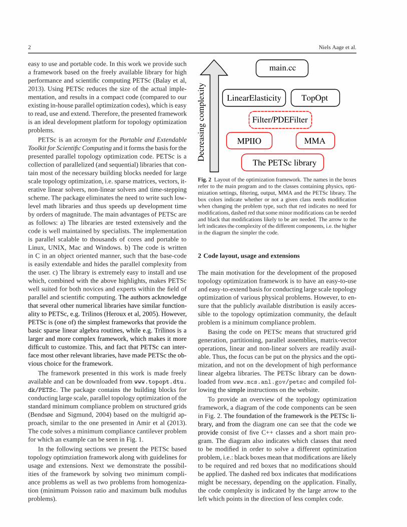
Fig. 2 Layout of the optimization framework. The names in the boxesrefer to the main program and to the classes containing physics, opti-mization settings, filtering, output, MMA and the PETSc library. Thebox colors indicate whether or not a given class needs modificationwhen changing the problem type, such that red indicates no need formodifications, dashed red that some minor modifications can be neededand black that modifications likely to be are needed. The arrow to theleft indicates the complexity of the different components,i.e. the higherin the diagram the simpler the code.

2 Code layout, usage and extensions

The main motivation for the development of the proposedtopology optimization framework is to have an easy-to-useand easy-to-extend basis for conducting large scale topologyoptimization of various physical problems. However, to en-sure that the publicly available distribution is easily acces-sible to the topology optimization community, the defaultproblem is a minimum compliance problem.

Basing the code on PETSc means that structured gridgeneration, partitioning, parallel assemblies, matrix-vectoroperations, linear and non-linear solvers are readily avail-able. Thus, the focus can be put on the physics and the opti-mization, and not on the development of high performancelinear algebra libraries. The PETSc library can be down-loaded fromwww.mcs.anl.gov/petsc and compiled fol-lowing thesimpleinstructions on the website.

To provide an overview of the topology optimizationframework, a diagram of the code components can be seenin Fig. 2.The foundation of the framework is the PETSc li-brary, and fromthe diagram one can see that the codeweprovideconsist of five C++ classes and a short main pro-gram. The diagram also indicates which classes that needto be modified in order to solve a different optimizationproblem, i.e.: black boxes mean that modifications are likelyto be required and red boxes that no modifications shouldbe applied. The dashed red box indicates that modificationsmight be necessary, depending on the application. Finally,the code complexity is indicated by the large arrow to theleft which points in the direction of less complex code.

Topology optimization using PETSc: 3

2.1 Class structure

Since the goal is to obtain a versatile framework, the classesare divided into clearly separated units. This means for ex-ample, that changing the physics only requires modificationsof a single class, i.e. the physics class which in the defaultcase solves a linear elasticity problem. A list of the classeswith description is given below

– TopOpt Contains information on the optimization prob-lem, gridsize, parameters and general settings.

– LinearElasticityThe physics class which solves thelinear elasticity problem on a structured 3D grid using8-node linear brick elements, see e.g. Zienkiewicz andTaylor (2000). It also contains methods necessary for theminimum compliance problem, i.e. objective, constraintand sensitivity calculations (Bendsøe and Sigmund, 2004).The default linear solver is a Galerkin projection multi-grid preconditioned flexible GMRES with GMRES/SORsmoothing, which follows the implementation presentedin Amir et al (2013), except for the choice of Krylovmethod and smoother. An example on how to changethe solver is given in the upcoming section.

– Filter/PDEFilterare filter classes which contains bothsensitivity (Sigmund, 1997), density (Bruns and Tortorelli,2001; Bourdin, 2001) and PDE (Lazarov and Sigmund,2011) filters through a common interface.

– MMAClass containing a fully parallelized implementationof the Method of Moving Asymptotes (MMA) (Svan-berg, 1987) following the description given in Aage andLazarov (2013).

– MPIIO A versatile output class capable of dumping arbi-trary field data into a single binary file.

The distribution also includesPythonscripts that convenientlyconverts the binary outputdata to the VTU format (Schroederet al, 2003) that can be visualized in e.g. ParaViewversion4 or newer(Ahrens et al, 2005).

2.2 Compiling and running the code

Assuming that PETSc is already installed (seewww.mcs.

anl.gov/petsc) the user is only required to perform thefollowing six steps to get started on a64-bitLinux platform1. Note that visualization of the results requires Python forpostprocessing and ParaView for the actual visualization.

1. Download and extract the code fromwww.topopt.dtu.dk/PETSc.

2. Modify themakefile such thatPETSC_DIR andPETSC_ARCH points to the local PETSc installation onyour system.

1 For other operating systems please follow the guidelines onwww.

mcs.anl.gov/petsc. After PETSc is installed, the compilation of theTopOpt application is done similar to that described in section 2.2.

3. Typemake topopt in a terminal to compile the code.4. Typempiexec -np 2 ./topopt to run the code on two

processors using the default settings. The optimizationand solver settings along with optimization history willbe written to the terminal.

5. Prepare the outputdata for ParaView by typingpython bin2vtu #, where # is the desired timestep.Note that the default settings saves data the first 10 itera-tions and then subsequently every 10th iteration in orderto save space.

6. Visualize in ParaView by typingparaview *.vtu.

The default problem is the minimum compliance cantileverproblem as described in Aage and Lazarov (2013) on a 2×1×1 domain using sensitivity filter with radius 0.08 and avolume fraction of 0.12 percent. The contrast between solidand void is set to 109, the convergence criteria is||xk −

xk−1||∞ < 0.01 or a maximum of 400 design cycles. Resultsbased on the default settings can be seen on the downloadpage.

2.3 Run time options

The flexibility of the framework allows the user to changea number of settings and parameters at run time. The opti-mization specific options that can be changed at run time arewritten to screen before the optimization begins, whereas thePETSc specific options, e.g. linear solver, can be found inthe PETSc manual. For example changing the filter to PDEfiltering with a radius of 0.2, a volume fraction of 0.3 and atotal of 200 iterationsis done inthe following command

mpiexec -np 2 ./topopt -filter 2 -rmin 0.2 \

-volfrac 0.3 -maxItr 200

Due to the flexible construction of PETSc it is possible tochange, monitor and test a vast variety of different solvercombinations simply by changing the run command. For ex-ample, changing the linear solver from the default to a Ja-cobi preconditioned conjugate gradient method can be ob-tained as follows

mpiexec -np 2 ./topopt -ksp_type cg \

-ksp_max_it 10000 -pc_type jacobi

However, using such a simple solver would result in in-creasedCPUtime, especially for large problems.

2.4 Extension

The list of possible extension that can be achieved, usingthe presented framework as a platform, covers everythingfrom linear to non-linear mechanics, fluid mechanics, acous-tics, electromagnetics and generalized multiphysics prob-lems. Describing all aspects of such extensions is outside

4 Niels Aage et al.

the scope of this paper, and we will therefore limit this sec-tion to discuss how to change the boundary conditions forthe minimum compliance problem and give a few generalguidelines for switching to a new physical setting.

To solve the minimum compliance problem with dif-ferent loading and support conditions, changes should onlybe made to a single method in the physics class, i.e. theSetUpLoadandBC()method inLinearElasticity.h/cc.This method simply sets the boundary conditions based oncoordinates and modifications are thereforestraightforward.

The modular composition of the optimization frameworkmeans that changing the physics to e.g. fluids, homogeniza-tion, etc, only requires that a single new class is written. Thecoding complexity is further minimized since much of theprovided linear elasticity solver can be reused or at leastprovide inspiration for the new physical problem. To demon-strate the versatility of the framework we alsoshow resultsfrom homogenization problems in the example section.

3 Examples

In the following sections the capabilities of the frameworkis presented by solving different minimum compliance prob-lems as well as material design problems for maximum bulkmodulus and minimum Poison’s ratio.Unless otherwise stated,all examples are run on a cluster with a total of 21 nodes,each equipped with two Intel Xeon 5650 6-core CPUs and48GB memory connected by Infiniband. All problems aresolved using theafore mentioned Galerkin projection ge-ometric multigrid preconditioned flexible-GMRES. If nototherwise stated we use four multigrid levels, four GMRES/SORsmoothing steps per level and a relative convergence toler-ance of 10−5. The coarse level problem is solved with GM-RES/SOR to 10−8 or a maximum of 30 iterations.Due tothe effectiveness of the multigrid preconditioning strategy,the F-GMRES is never restarted,i.e. for the presented ex-amples all linear solves are obtained with much less thanthe allowed 200 F-GMRES iterations.

3.1 Minimum compliance

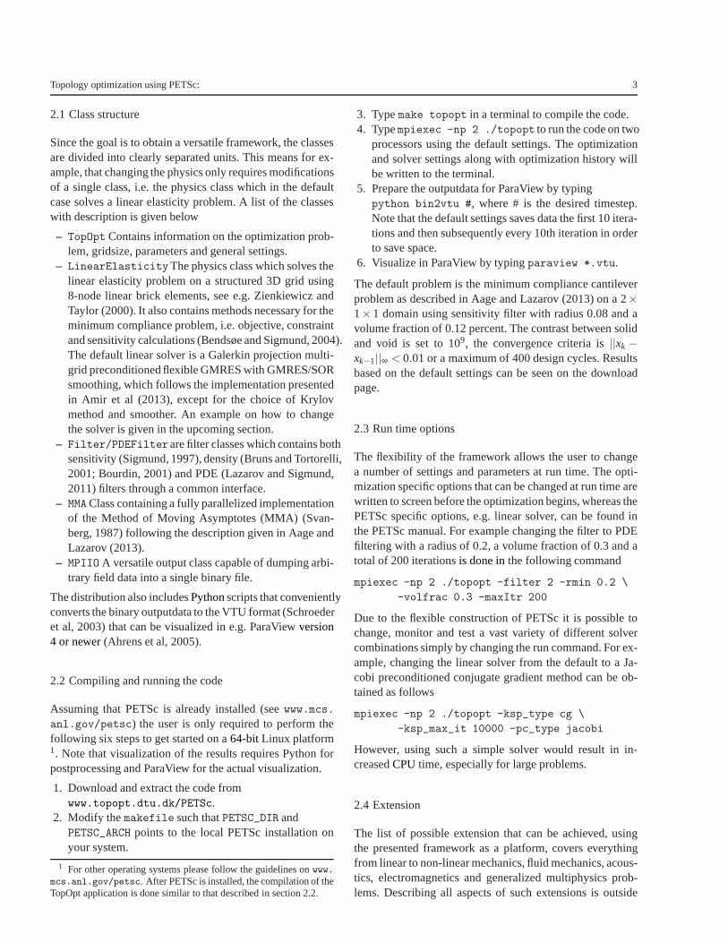
The first example is a re-run of the cantilever problem pre-sented in (Aage and Lazarov, 2013). In this work we dis-cretize the 2×1×1 cantilever by 480×240×240 elements,i.e. 27.6 million design elements and 83.8 million state dofs.The problem is then solved for various filter radii, i.e. fromrmin = 0.01 to 0.1, with a solid/void contrast of 109. Thedesign problemshave been runfor 1000 design iterationson 24 CPUs (144 cores) yielding an average iteration timevarying from 60s to 30s for the smallest and largest filter ra-dius, respectively. The relationship between lengthscaleand

(a) (b)

(c) (d)

(e) (f)

Fig. 3 Optimized cantilever beams on a 2× 1× 1 domain allowing12% material discretized by 27.6 million elements. The design prob-lems differ through the filter radius such thatrmin = 0.01 for (a,c),rmin = 0.03 for (b,d),rmin = 0.04 for (e) andrmin = 0.10 for (f). Plot(c) and (d) shows cross sections of the designs withrmin = 0.01 and0.03, and illustrates the internal holes generated for the smaller filterradius. All the designs are thresholded atρPhys= 0.5 and colored bythe magnitude of the displacement field.

solution time (i.e. number of iterations for GMRES) is ex-pected for the chosen multigrid preconditioner, since smallerlengthscales are harder to represent on the coarse grids. Theoptimized designs can be seen in Fig. 3. It is especially inter-esting to note that the high design resolution and small filterradius, leads to a design where the beams contain internalholes.

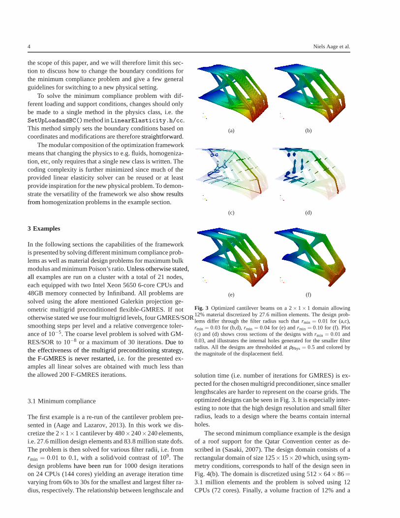
The second minimum compliance example is the designof a roof support for the Qatar Convention center as de-scribed in (Sasaki, 2007). The design domain consists of arectangular domain of size 125×15×20 which, using sym-metry conditions, corresponds to half of the design seen inFig. 4(b). The domain is discretized using 512×64×86=3.1 million elements and the problem is solved using 12CPUs (72 cores). Finally, a volume fraction of 12% and a

Topology optimization using PETSc: 5

(a)

(b)

Fig. 4 Minimum compliance design of a roof support, c.f. the QatarConvention center (Sasaki, 2007). The plot in (a) shows the full op-timized roof structure, while plot (b) shows a single of the two sup-port structures. The design domain is due to symmetry reduced to onequarter of the domain seen in (a) or half of (b). The computationalmesh consists of 3.1 million elements. Both plots are thresholded atρPhys= 0.5 and colored by the density field.

filter radius ofrmin = 3.0 is used to obtain the design shownin Fig. 4. The design of the roof support requires two ex-tensions to the default code: First a passive solid domainof size 125× 15× 1, i.e. the roof, is introduced and sec-ondly a Heaviside projection continuation method (Guestet al, 2004) is necessary due to the large filter radius usedfor the PDE filter.

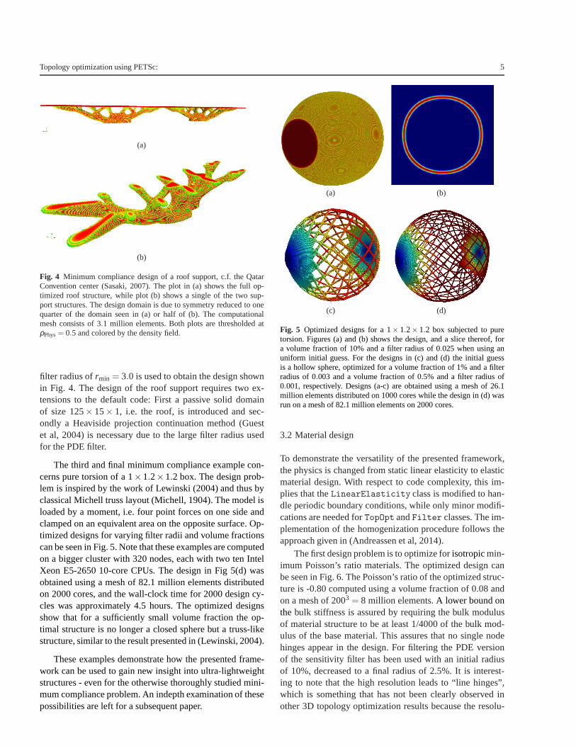
The third and final minimum compliance example con-cerns pure torsion of a 1×1.2×1.2 box. The design prob-lem is inspired by the work of Lewinski (2004) and thus byclassical Michell truss layout (Michell, 1904). The model isloaded by a moment, i.e. four point forces on one side andclamped on an equivalent area on the opposite surface. Op-timized designs for varying filter radii and volume fractionscan be seen in Fig. 5. Note that these examples are computedon a bigger cluster with 320 nodes, each with two ten IntelXeon E5-2650 10-core CPUs. The design in Fig 5(d) wasobtained using a mesh of 82.1 million elements distributedon 2000 cores, and the wall-clock time for 2000 design cy-cles was approximately 4.5 hours. The optimized designsshow that for a sufficiently small volume fraction the op-timal structure is no longer a closed sphere but a truss-likestructure, similar to the result presented in (Lewinski, 2004).

These examples demonstrate how the presented frame-work can be used to gain new insight into ultra-lightweightstructures - even for the otherwise thoroughly studied mini-mum compliance problem. An indepth examination of thesepossibilities are left for a subsequent paper.

(a) (b)

(c) (d)

Fig. 5 Optimized designs for a 1× 1.2× 1.2 box subjected to puretorsion. Figures (a) and (b) shows the design, and a slice thereof, fora volume fraction of 10% and a filter radius of 0.025 when using anuniform initial guess. For the designs in (c) and (d) the initial guessis a hollow sphere, optimized for a volume fraction of 1% and afilterradius of 0.003 and a volume fraction of 0.5% and a filter radius of0.001, respectively. Designs (a-c) are obtained using a mesh of 26.1million elements distributed on 1000 cores while the designin (d) wasrun on a mesh of 82.1 million elements on 2000 cores.

3.2 Material design

To demonstrate the versatility of the presented framework,the physics is changed from static linear elasticity to elasticmaterial design. With respect to code complexity, this im-plies that theLinearElasticity class is modified to han-dle periodic boundary conditions, while only minor modifi-cations are needed forTopOpt andFilter classes. The im-plementation of the homogenization procedure follows theapproach given in (Andreassen et al, 2014).

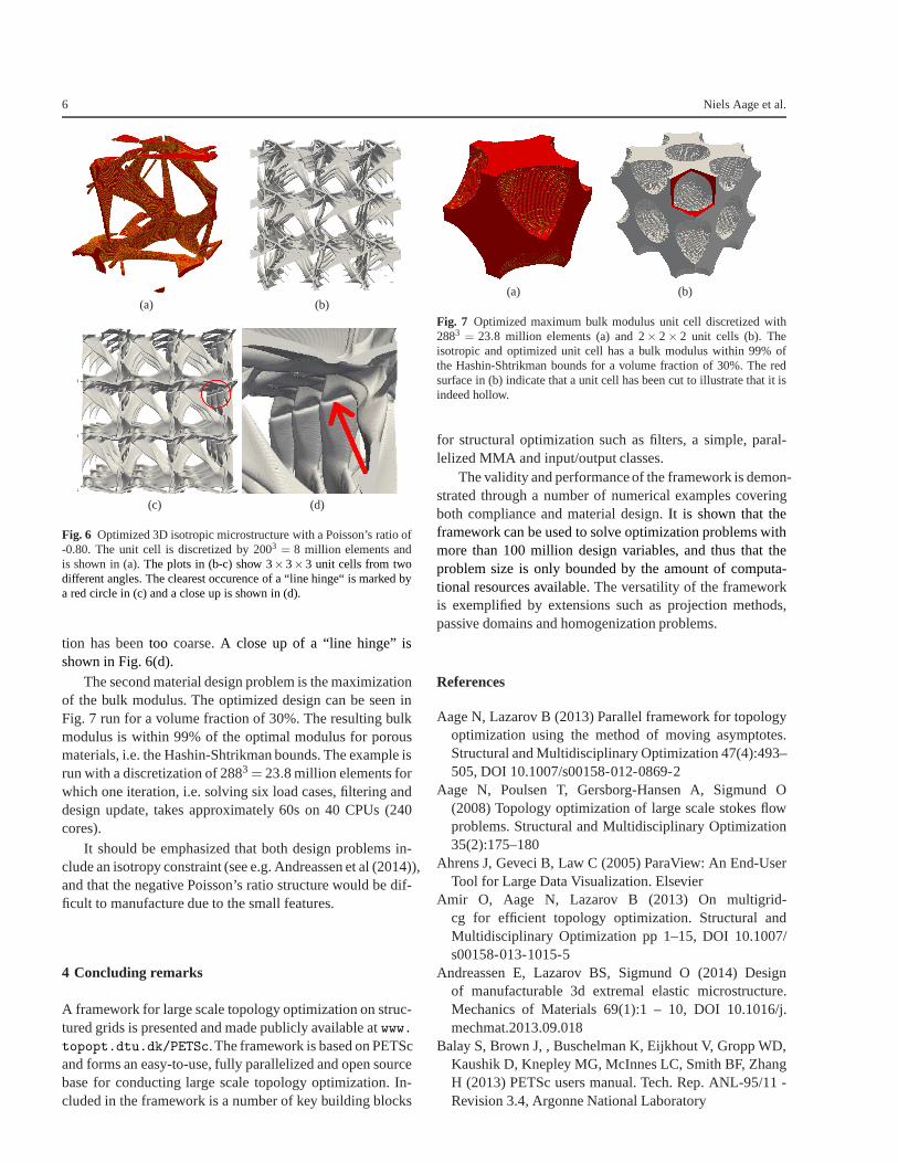
The first design problem is to optimize forisotropicmin-imum Poisson’s ratio materials. The optimized design canbe seen in Fig. 6. The Poisson’s ratio of the optimized struc-ture is -0.80 computed using a volume fraction of 0.08 andon a mesh of 2003 = 8 million elements.A lower bound onthebulk stiffness is assured by requiring the bulk modulusof material structure to be at least 1/4000 of the bulk mod-ulus of the base material. This assures that no single nodehinges appear in the design. For filtering the PDE versionof the sensitivity filter has been used with an initial radiusof 10%, decreased to a final radius of 2.5%. It is interest-ing to note that the high resolution leads to “line hinges”,which is something that has not been clearly observed inother 3D topology optimization results because the resolu-

6 Niels Aage et al.

(a) (b)

(c) (d)

Fig. 6 Optimized 3D isotropic microstructure with a Poisson’s ratio of-0.80. The unit cell is discretized by 2003

= 8 million elements andis shown in (a).The plots in (b-c) show 3×3×3 unit cells from twodifferent angles. The clearest occurence of a “line hinge“ is marked bya red circle in (c) and a close up is shown in (d).

tion has beentoo coarse.A close up of a “line hinge” isshown in Fig. 6(d).

The second material design problem is the maximizationof the bulk modulus. The optimized design can be seen inFig. 7 run for a volume fraction of 30%. The resulting bulkmodulus is within 99% of the optimal modulus for porousmaterials, i.e. the Hashin-Shtrikman bounds. The example isrun with a discretization of 2883 = 23.8 million elements forwhich one iteration, i.e. solving six load cases, filtering anddesign update, takes approximately 60s on 40 CPUs (240cores).

It should be emphasized that both design problems in-clude an isotropy constraint (see e.g. Andreassen et al (2014)),and that the negative Poisson’s ratio structure would be dif-ficult to manufacture due to the small features.

4 Concluding remarks

A framework for large scale topology optimization on struc-tured grids is presented and made publicly available atwww.

topopt.dtu.dk/PETSc.The framework is based on PETScand forms an easy-to-use, fully parallelized and open sourcebase for conducting large scale topology optimization. In-cluded in the framework is a number of key building blocks

(a) (b)

Fig. 7 Optimized maximum bulk modulus unit cell discretized with2883

= 23.8 million elements (a) and 2× 2× 2 unit cells (b). Theisotropic and optimized unit cell has a bulk modulus within 99% ofthe Hashin-Shtrikman bounds for a volume fraction of 30%. The redsurface in (b) indicate that a unit cell has been cut to illustrate that it isindeed hollow.

for structural optimization such as filters, a simple, paral-lelized MMA and input/output classes.

The validity and performance of the framework is demon-strated through a number of numerical examples coveringboth compliance and material design.It is shown that theframework can be used to solve optimization problems withmore than 100 million design variables, and thus that theproblem size is only bounded by the amount of computa-tional resources available.The versatility of the frameworkis exemplified by extensions such as projection methods,passive domains and homogenization problems.

References

Aage N, Lazarov B (2013) Parallel framework for topologyoptimization using the method of moving asymptotes.Structural and Multidisciplinary Optimization 47(4):493–505, DOI 10.1007/s00158-012-0869-2

Aage N, Poulsen T, Gersborg-Hansen A, Sigmund O(2008) Topology optimization of large scale stokes flowproblems. Structural and Multidisciplinary Optimization35(2):175–180

Ahrens J, Geveci B, Law C (2005) ParaView: An End-UserTool for Large Data Visualization. Elsevier

Amir O, Aage N, Lazarov B (2013) On multigrid-cg for efficient topology optimization. Structural andMultidisciplinary Optimization pp 1–15, DOI 10.1007/s00158-013-1015-5

Andreassen E, Lazarov BS, Sigmund O (2014) Designof manufacturable 3d extremal elastic microstructure.Mechanics of Materials 69(1):1 – 10, DOI 10.1016/j.mechmat.2013.09.018

Balay S, Brown J, , Buschelman K, Eijkhout V, Gropp WD,Kaushik D, Knepley MG, McInnes LC, Smith BF, ZhangH (2013) PETSc users manual. Tech. Rep. ANL-95/11 -Revision 3.4, Argonne National Laboratory

Topology optimization using PETSc: 7

Bendsøe M, Sigmund O (2004) Topology Optimization;Theory, Methods and Applications, 2nd edn. SpringerVerlag Berlin Heidelberg New York

Borrvall T, Petersson J (2001) Large-scale topology op-timization in 3d using parallel computing. ComputerMethods in Applied Mechanics and Engineering 190(46-47):6201–6229

Bourdin B (2001) Filters in topology optimization. Int J Nu-mer Meth Engng 50(9):2143–2158

Bruns TE, Tortorelli DA (2001) Topology optimization ofnon-linear elastic structures and compliant mechanisms.Computer Methods in Applied Mechanics and Engineer-ing 190(26-27):3443–3459

Challis V, Roberts A, Grotowski J (2013) High resolutiontopology optimization using graphics processing units(GPUs). Structural and Multidisciplinary Optimization pp1–11, DOI 10.1007/s00158-013-0980-z

Evgrafov A, Rupp CJ, Maute K, Dunn ML (2008) Large-scale parallel topology optimization using a dual-primalsubstructuring solver. Structural And MultidisciplinaryOptimization 36(4):329–345

Guest JK, Prevost JH, Belytschko T (2004) Achievingminimum length scale in topology optimization usingnodal design variables and projection functions. Inter-national Journal For Numerical Methods In Engineering61(2):238–254

Heroux MA, Bartlett RA, Howle VE, Hoekstra RJ, Hu JJ,Kolda TG, Lehoucq RB, Long KR, Pawlowski RP, PhippsET, Salinger AG, Thornquist HK, Tuminaro RS, Willen-bring JM, Williams A, Stanley KS (2005) An overview ofthe trilinos project. ACM Trans Math Softw 31(3):397–423, DOI http://doi.acm.org/10.1145/1089014.1089021

Kim TS, Kim JE, Kim YY (2004) Parallelized structuraltopology optimization for eigenvalue problems. Interna-tional Journal of Solids and Structures 41(9-10):2623–2641

Lazarov BS, Sigmund O (2011) Filters in topology opti-mization based on helmholtz-type differential equations.International Journal For Numerical Methods In Engi-neering

Lewinski T (2004) Michell structures formed on surfaces ofrevolution. Structural and Multidisciplinary Optimization28(1):20–30, DOI 10.1007/s00158-004-0419-7

Mahdavi A, Balaji R, Frecker M, Mockensturm EM (2006)Topology optimization of 2D continua for minimum com-pliance using parallel computing. Structural And Multi-disciplinary Optimization 32(2):121–132

Michell AGM (1904) The limits of economy of materials inframe structures. DOI 10.1080/14786440409463229

Sasaki M (2007) Morphogenesis of Flux Structure. Archi-tectural Association Publications London

Schmidt S, Schulz V (2011) A 2589 line topology opti-mization code written for the graphics card. Comput-

ing and Visualization in Science 14(6):249–256, DOI10.1007/s00791-012-0180-1

Schroeder W, Martin K, Lorensen B (2003) The Visualiza-tion Toolkit, Third Edition. Kitware Inc.

Sigmund O (1997) On the design of compliant mechanismsusing topology optimization. Mechanics of Structures andMachines 25(4):493–525

Svanberg K (1987) The method of moving asymptotes -a new method for structural optimization. InternationalJournal for Numerical Methods in Engineering 25

Vemaganti K, Lawrence WE (2005) Parallel methods for op-timality criteria-based topology optimization. ComputerMethods in Applied Mechanics and Engineering 194(34-35):3637–3667

Wadbro E, Berggren M (2009) Megapixel topology opti-mization on a graphics processing unit. SIAM Review51(4):707–721

Zienkiewicz OC, Taylor RL (2000) Finite Element Method:Volume 1, 5th edn. Butterworth-Heinemann