topological vertex and quantum mirror curveskanehisa.takasaki/res/ocu1511slide.pdf · topological...

Topological vertex

and quantum mirror curves

Kanehisa Takasaki, Kinki University

Osaka City University, November 6, 2015

Contents1. Topological vertex2. On-strip geometry3. Closed topological vertex

Based on1. K. T., arXiv:1301.4548 [math-ph]2. K. T. and T. Nakatsu, arXiv:1507.07053

1

1. Topological vertex

Web diagrams of non-compact toric Calabi-Yau threefolds

On-strip geometryClosed topological vertex

Topological vertex

“Topological vertex” (Aganagic, Klemm, Marino and Vafa 2003)is a diagrammatic method to construct the partition functions(or amplitudes) of topological string theory on non-compacttoric Calabi-Yau threefolds.

2


Vertex weight

Cλµν = qκ(µ)/2s tν(q−ρ)∑η∈P

s tλ/η(q−ν−ρ)sµ/η(q−tν−ρ)

• λ = (λi)∞i=1, µ = (µi)∞i=1, ν = (νi)∞i=1 arepartitions representing Young diagrams ofarbitrary shapes. tν denotes the conjugatepartition of ν.

λ µ

ν

• κ(µ) is the second Casimir invariant

κ(µ) =∞∑i=1

µi(µi − 2i+ 1) = 2∑

(i,j)∈µ

(j − i)

3


Vertex weight (cont’d)

Cλµν = qκ(µ)/2s tν(q−ρ)∑η∈P

s tλ/η(q−ν−ρ)sµ/η(q−tν−ρ)

• s tν(q−ρ), s tλ/η(q−ν−ρ) and sµ/η(q−tν−ρ) are special values

of the Schur/skew Schur functions s tν(x), s tλ/η(x), sµ/η(x),x = (x1, x2, · · · ), at

q−ρ = (qi−1/2)∞i=1, q−ν−ρ = (q−νi+i−1/2)∞i=1,

q−tν−ρ = (q−

tνi+i−1/2)∞i=1

• Vertex weights are glued together along the internal lines.Edge weights are assigned to those lines.

4


Examples (local P1 geometry)

1. Open string amplitudes of X = O(−1)⊕O(−1) → CP1 (resolved conifold):

Zα0α2β1β2

=∑

α1∈PCα1α0β1(−Q)|α1|C tα1α2β2

2. Open string amplitudes of X = O ⊕O(−2) → CP1:

Zα0α2β1β2

=∑

α1∈PCα1α0β1(−Q)|α1|

× (−1)|α1|q−κ(α1)/2Cα2tα1β2

(A framing factor is inserted in this case.)

β1

β2

α0

α2

α1,Q

β1

β2

α0

α2

α1,Q

5


Building blocks of operator formalism

• Charge-zero sector of fermionic Fock space spanned by theground states 〈0|, |0〉 and the excited states

〈λ| = 〈−∞| · · ·ψ∗λi−i+1 · · ·ψ∗

λ2−1ψ∗λ1,

|λ〉 = ψ−λ1ψ−λ2+1 · · ·ψ−λi+i−1 · · · | −∞〉

• Fermion bilinears

L0 =∑n∈Z

n:ψ−nψ∗n:, K =

∑n∈Z

(n− 1/2)2:ψ−nψ∗n:,

Jm =∑n∈Z

:ψm−nψ∗n:, m ∈ Z,

V (k)m = q−km/2

∑n∈Z

qkn:ψm−nψ∗n:, k,m ∈ Z.

6


• Vertex operators

Γ±(z) = exp

( ∞∑k=1

zk

kJ±k

), Γ′

±(z) = exp

(−

∞∑k=1

(−z)k

kJ±k

)and the multi-variable extensions

Γ±(x) =∏i≥1

Γ±(xi), Γ′±(x) =

∏i≥1

Γ′±(xi)

Fermionic expression of vertex weight

Cλµν = s tν(q−ρ)〈 tλ|Γ−(q−ν−ρ)Γ+(q−tν−ρ)qK/2|µ〉

= s tν(q−ρ)〈λ|Γ′−(q−ν−ρ)Γ′

+(q−tν−ρ)q−K/2| tµ〉

(Okounkov, Reshetikhin and Vafa 2003)

7


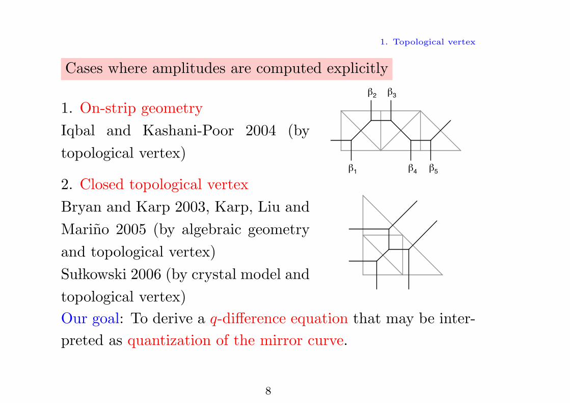
Cases where amplitudes are computed explicitly

1. On-strip geometryIqbal and Kashani-Poor 2004 (bytopological vertex)

β1

β2

β3

β4

β5

2. Closed topological vertexBryan and Karp 2003, Karp, Liu andMarino 2005 (by algebraic geometryand topological vertex)Su lkowski 2006 (by crystal model andtopological vertex)Our goal: To derive a q-difference equation that may be inter-preted as quantization of the mirror curve.

8

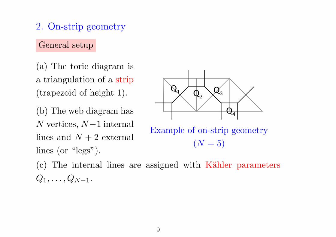
2. On-strip geometry

General setup

(a) The toric diagram isa triangulation of a strip(trapezoid of height 1).

(b) The web diagram hasN vertices, N−1 internallines and N + 2 externallines (or “legs”).

Q1 Q

2

Q3

Q4

Example of on-strip geometry(N = 5)

(c) The internal lines are assigned with Kahler parametersQ1, . . . , QN−1.

9


General setup (cont’d)

(d) The external lines areassigned with partitionsα0, β1, . . . , βN , αN .

(e) The sign (or type) σn

of the n-th vertical legare defined as

σn =

+1 if the leg points ↑

−1 if the leg points ↓

β2

β3

β1

β4

β5

α0

α5

σ2 = σ3 = +1,σ1 = σ4 = σ5 = −1

Let Zα0αNβ1...βN

denote the open string amplitude constructed bytopological vertex.

10


Infinite-product formula of amplitude

If α0 = αN = ∅, the amplitude can be computed explicitlywith the aid of the Cauchy identities for skew Schur functions(Iqbal and Kashani-Poor 2004):

Z∅∅β1···βN

= s tβ1(q−ρ) · · · s tβN

(q−ρ)

×∏

1≤m<n≤N

∞∏i,j=1

(1 −Qmnq− tβ

(m)i −β

(n)j +i+j−1)−σmσn

where

β(n) =

βn if σn = +1,tβn if σn = −1,

Qmn = QmQm+1 · · ·Qn−1

11


Fermionic expression of amplitude

The infinite-product formula holds only for α0 = αN = ∅. Forgeneral cases, the following fermionic expression is available:

Zα0αNβ1···βN

= q(1−σ1)κ(α0)/4q(1+σN )κ(αN )/4s tβ1(q−ρ) · · · s tβN

(q−ρ)

× 〈 tα0|Γσ1− (q−β(1)−ρ)Γσ1

+ (q−tβ(1)−ρ)(σ1Q1σ2)L0 · · ·

× ΓσN−1− (q−β(N−1)−ρ)ΓσN−1

+ (q−tβ(N−1)−ρ)(σN−1QN−1σN )L0

× ΓσN− (q−β(N)−ρ)ΓσN

+ (q−tβ(N)−ρ)|αN 〉

where Γσ± denote Γ± if σ = +1 and Γ′

± if σ = −1 (Eguchi andKanno 2003, Bryan and Young 2008 for special cases; Nagao2009 and Su lkowski 2009 for general cases)

12


Wave functions

Wave functions are defined as

Ψn(x) =∞∑

k=0

Zn,(1k)

Zn,∅xk, Ψn(x) =

∞∑k=0

Zn,(k)

Zn,∅xk

for n = 0, 1, . . . , N,N + 1, where

Z0,λ = Zλ∅∅···∅, Zn,λ = Z∅∅

···∅λ∅··· (1 ≤ n ≤ N), ZN+1,λ = Z∅λ∅···∅

Remark: Zn,λ’s are the coefficients of Schur function expansionof a KP tau function τn. In this sense, these wave functionsare Baker-Akhiezer functions (at the initial time t = 0) thatcorrespond to free fermion fields ψ(−x), ψ∗(x).

13


Ψn and Ψn for n = 1, . . . , N are q-hypergeometric series

Ψn(x) = 1+∞∑

k=1

Cn(1)Cn(q) · · ·Cn(qk−1)Bn(1)Bn(q) · · ·Bn(qk−1)(1 − q) · · · (1 − qk)

qk/2xk

where Bn(y) and Cn(y) are Laurent polynomials in y:

Bn(y) =∏

m<n, σmσn>0

(1 −Qmnyσn) ×

∏m>n, σmσn>0

(1 −Qnmy−σn),

Cn(y) =∏

m<n, σmσn<0

(1 −Qmnyσn) ×

∏m>n, σmσn<0

(1 −Qnmy−σn)

Remark: When N = 1, Ψ reduces to a quantum dilog:

Ψ(x) = 1 +∞∑

k=1

qk/2xk

(1 − q) · · · (1 − qk)=

∞∏i=1

(1 − qi−1/2x)−1

14


Ψ1, . . . ,ΨN satisfy q-difference equation

Ψn(x) − Ψn(qx) = q1/2xCn(qx∂x)Bn(qx∂x)

Ψn(x)

or, equivalently,

Bn(q−1qx∂x)(1 − qx∂x)Ψn(x) = q1/2xCn(qx∂x)Ψn(x)

(Kashani-Poor 2006, Hyun and Yi 2006, Gukov and Su lkowski2011 for the resolved conifold).

Remark: These equations are also studied in the context of theAGT correspondence (Kozcaz, Pasquetti and Wyllard 2010,Taki 2010) and the vortex partition function (Bonelli, Tanziniand Zhao 2011).

15


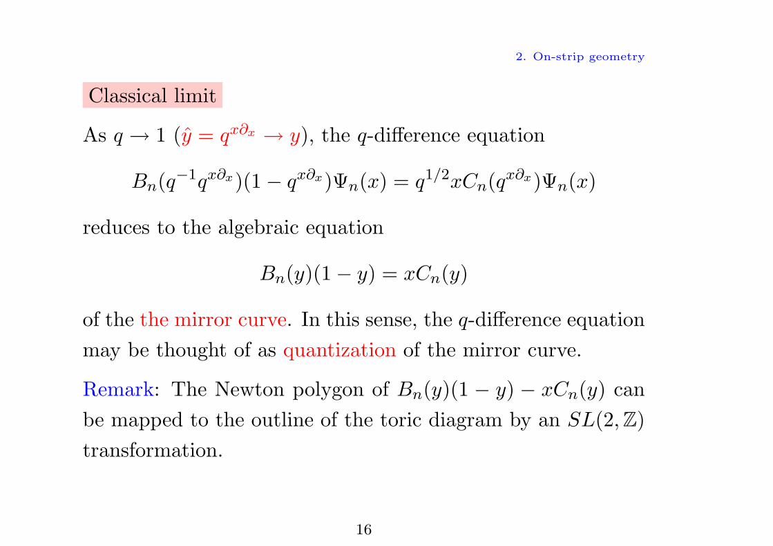
Classical limit

As q → 1 (y = qx∂x → y), the q-difference equation

Bn(q−1qx∂x)(1 − qx∂x)Ψn(x) = q1/2xCn(qx∂x)Ψn(x)

reduces to the algebraic equation

Bn(y)(1 − y) = xCn(y)

of the the mirror curve. In this sense, the q-difference equationmay be thought of as quantization of the mirror curve.

Remark: The Newton polygon of Bn(y)(1 − y) − xCn(y) canbe mapped to the outline of the toric diagram by an SL(2,Z)transformation.

16


How the equations for different n’s are related

x = (1 − y)Bn(y)Cn(y)

(♥)−→ x = (1 − y)Bn+1(y)Cn+1(y)

(♥) y = Qσnn yσnσn+1 , x = g(y, y)xσnσn+1

where

g(y, y) =

−y−1 if σn = +1, σn+1 = +1,

1 if σn = +1, σn+1 = −1,

yy if σn = −1, σn+1 = +1,

−y if σn = −1, σn+1 = −1

Birational map (♥) preserves the symplectic structure:

d log x ∧ d log y = d log x ∧ d log y

17


What about Ψ0 and ΨN+1 ?

They are related to quantum dilogs. E.g., if σ1 = +1, Ψ0(x) isa product of quantum dilogs and satisfies the equation

Ψ0(qx) = (1 − q1/2x)−1N∏

n=2

(1 −Qn−1q1/2x)−σnΨ0(x).

Its classical limit is the algebraic equation

y = (1 − x)−1N∏

n=2

(1 −Qn−1x)−σn .

This equation can be transformed to the equation x = (1 −y)B1(y)/C1(y) by a birational symplectic map (x, y) 7→ (x, y):d log y ∧ d log x = d log x ∧ d log y.

18

3. Closed topological vertex

Setup

(a) Three internal linesare assigned with Kahlerparameters Q1, Q2, Q3

(b) Two vertical externallines are assigned withpartitions β1, β2. Allother external lines aregiven ∅.

Q2

β1

β2

Q1

Q3

Let Zctvβ1β2

denote the open string amplitude in this setting.

19


Method of computation of Zctvβ1β2

• Reconstruct the amplitudeZctv

β1β2by gluing a single vertex

C tα∅∅ to the amplitude of anon-strip geometry.

• Borrow tools from our previ-ous study on integrable struc-tures of the melting crystalmodels (5D U(1) instanton sumand its variants) (Nakatsu andK.T, since 2007) to computethe sum over α ∈ P.

tα

β1

β2

α

Q3

Gluing a vertex (top) to anon-strip geometry (bottom)

20


Result of computation of Zctvβ1β2

Zctvβ1β2

= qκ(β2)/2∞∏

i,j=1

(1 −Q1Q2q−β1i− tβ2j+i+j−1)−1

× 〈 tβ1|Γ−(q−ρ)Γ+(q−ρ)(−Q1)L0Γ′−(q−ρ)Γ′

+(q−ρ)(−Q3)L0

× Γ−(q−ρ)Γ+(q−ρ)(−Q2)L0Γ′−(q−ρ)Γ′

+(q−ρ)| tβ2〉.

• The main part Yβ1β2 := 〈 tβ1| · · · | tβ2〉 is essentially the openstring amplitude of yet another on-strip geometry. This strangecoincidence is a key to derive a q-difference equation.

• Letting β1 = β2 = ∅, this expression reduces to the knownresult of the closed string amplitudes (Bryan and Karp 2003,Karp, Liu and Marino 2005).

21


Wave functions

Wave functions are defined as

Ψ(x) =∞∑

k=0

Zctv(1k)∅

Zctv∅∅

xk, Ψ(x) =∞∑

k=0

Zctv(k)∅

Zctv∅∅

xk

along with the auxiliary wave functions

Φ(x) =∞∑

k=0

Y(1k)∅

Y∅∅xk, Φ(x) =

∞∑k=0

Y(k)∅

Y∅∅xk

obtained from the main part Yβ1β2 = 〈 tβ1| · · · | tβ2〉 of Zctvβ1β2

.

22


Wave functions (cont’d)

• The coefficients of Ψ(x) =∞∑

k=0

akxk and Φ(x) =

∞∑k=0

bkxk,

a0 = b0 = 1, are related as

ak = bk

k∏i=1

(1 −Q1Q2qi−1)−1

• Φ(x) is build from quantum dilogs, and satisfies the q-differenceequation

Φ(qx) =(1 − q1/2x)(1 −Q1Q3q

1/2x)(1 −Q1q1/2x)(1 −Q1Q2Q3q1/2x)

Φ(x).

23


Transforming q-difference equation

The q-difference equation

(1 −Q1q1/2x)(1 −Q1Q2Q3q

1/2x)Φ(qx)

= (1 − q1/2x)(1 −Q1Q3q1/2x)Φ(x)

for Φ(x) is transformed to the q-difference equation

(1 −Q1Q2q−2qx∂x −Q1q

1/2x)(1 −Q1Q2q−1qx∂x −Q1Q2Q3q

1/2x)Ψ(qx)

= (1 −Q1Q2q−2qx∂x − q1/2x)(1 −Q1Q2q

−1qx∂x −Q1Q3q1/2x)Ψ(x)

for Ψ(x). Let us rewrite this equation as

H(x, qx∂x)Ψ(x) = 0

and examine the q-difference operator H(x, qx∂x).

24


Reducing q-difference equation to final form

The operator H(x, qx∂x) can be factorized as

H(x, qx∂x) = (1 −Q1Q2q−2qx∂x)K(x, qx∂x)

where

K(x, qx∂x) = (1 −Q1Q2q−1qx∂x)(1 − qx∂x) − (1 +Q1Q3)q1/2x

+Q1(1 +Q2Q3)q1/2xqx∂x +Q1Q3qx2.

Since the prefactor 1−Q1Q2q−2qx∂x is invertible on the space

of power series of x, the equation H(x, qx∂x)Ψ(x) = 0 reducesto

K(x, qx∂x)Ψ(x) = 0

This is the final form of our quantum mirror curve.

25


Classical limit

As q → 1, the q-difference operator

K(x, qx∂x) = (1 −Q1Q2q−1qx∂x)(1 − qx∂x) − (1 +Q1Q3)q1/2x

+Q1(1 +Q2Q3)q1/2xqx∂x +Q1Q3qx2

turns into the polynomial

Kcl(x, y) = (1 −Q1Q2y)(1 − y) − (1 +Q1Q3)x

+Q1(1 +Q2Q3)xy +Q1Q3x2

Its Newton polygon has the same shape as the triangular out-line of the toric diagram.

26


What about wave functions obtained from β2 = (k), (1k) ?

The q-difference equations become slightly more complicatedbecause of the framing factor qκ(β2)/2.

What about putting β1 and β2 on other legs ?

The open string amplitude can be expressed in a similar form.However qK/2’s remain in the operator product, and they pre-vent us from doing explicit computation. A similar difficultytakes place when one attempts to prolong the branches of theclosed topological vertex.

What about web diagrams with cycle(s) ?

It is an ultimate goal of our project, but we have currently noidea.

27

topological vertex and quantum mirror curveskanehisa.takasaki/res/ocu1511slide.pdf · topological...

Documents