topics in - ihesvanhove/slides/deruelle-ihes-apr2010.pdf · topics in f(r) theories of gravity...
TRANSCRIPT
1
Topics in
f(R) THEORIES OF GRAVITY
Nathalie Deruelle
APC-CNRS, Paris
ihes, April 22th 2010

2
INTRODUCTION
The observed universe is well represented by a Friedmann-Lemaıtre spacetimethe scale factor of which started to accelerate recently
No Big Bang
1 2 0 1 2 3
expands forever
-1
0
1
2
3
2
3
closed
recollapses eventually
Supernovae
CMB
Clusters
open
flat
Knop et al. (2003)Spergel et al. (2003)Allen et al. (2002)
Supernova Cosmology Project
Ω
ΩΛ
M
ds2 = gijdxidxj = −dt2 + a2(t)dσ2k
Gij = κ T totalij ; DjT
ij = 0
H2 + ka2 = κ
3ρtotal ; H = 1a
dadt(
HH0
)2
= Ω0rad
(a0a
)4 + Ω0mat
(a0a
)3 + Ω0k
(a0a
)2 + Ω0Λ
H0 ≈ 70 ; Ω0rad ≈ 10−4 ; Ω0
mat ≈ 0.3 , Ω0k ≈ 0
Ω0Λ ≈ 0.7 : Dark Energy
=⇒ κTΛij = −Λgij , a(t)→ e
√Λ/3 t , Λ = 3Ω0
ΛH20

3
Origin of this acceleration
• An artefact of the averaging process ?
Gij(<gkl>) = κ <Tij > instead of <Gij(gkl)>= κ <Tij >G(<gkl>) 6=<G(gkl)>) Ellis, 1971,..., see review Buchert, 2006 et seq.
• Exotic matter ? (ρΛ + pΛ ≈ 0)
– Chaplygin gas : pρ = −A, (Kamenshchik et al., 2001)– Quintessence : R.G. plus ϕ with V ∝ 1/ϕn (Steinhardt et al., 1997)
• “Modified” gravity ?
– Λ : the simplest explanation, (Bianchi and Rovelli, Feb 2010)– MOND, see, e.g., Navarro and Acoleyen, 2005– “Branes” : DGP (2000), Deffayet (2001)– f(R) lagrangian, instead of Hilbert’s R
C.D.T.T. (2003), Capozziello et al. (2003)

4
Outline of the talk
1. Introducing f(R) theories of gravity
or : f(R) theories as scalar-tensor theories of gravity
2. f(R) cosmological models of dark energyor : the search for viable models
3. f(R) gravity and local testsor : how to hide the scalar d.o.f. of gravity
4. Back to cosmological modelsor : how to hide the scalar d.o.f. of gravity
5. Remarks on Black Holes in f(R) theories
(uniqueness and thermodynamics)
5
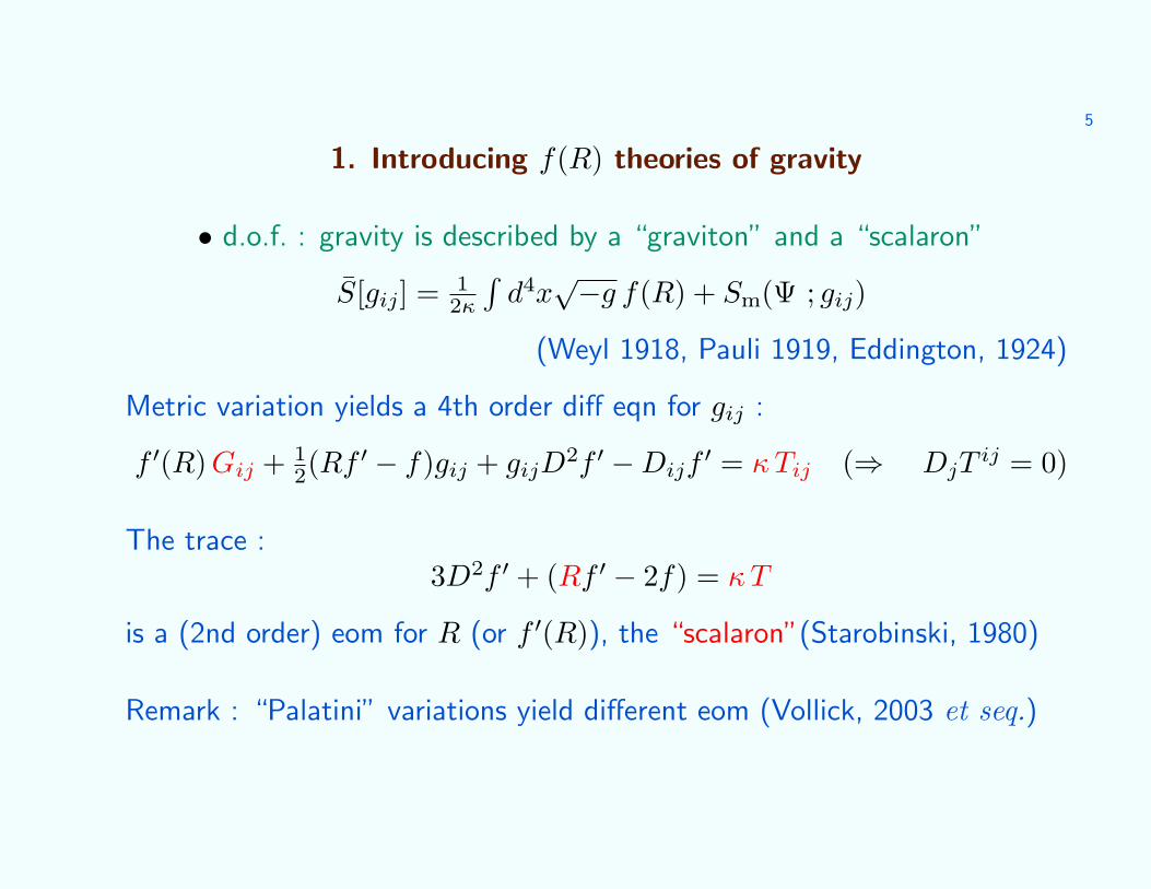
1. Introducing f(R) theories of gravity
• d.o.f. : gravity is described by a “graviton” and a “scalaron”
S[gij] = 12κ
∫d4x√−g f(R) + Sm(Ψ ; gij)
(Weyl 1918, Pauli 1919, Eddington, 1924)
Metric variation yields a 4th order diff eqn for gij :
f ′(R) Gij + 12(Rf ′ − f)gij + gijD
2f ′ −Dijf′ = κ Tij (⇒ DjT
ij = 0)
The trace :3D2f ′ + (Rf ′ − 2f) = κ T
is a (2nd order) eom for R (or f ′(R)), the “scalaron”(Starobinski, 1980)
Remark : “Palatini” variations yield different eom (Vollick, 2003 et seq.)
6
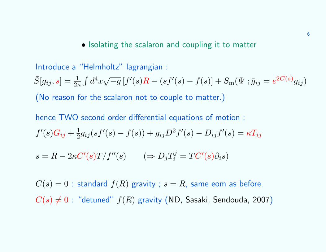
• Isolating the scalaron and coupling it to matter
Introduce a “Helmholtz” lagrangian :
S[gij, s] = 12κ
∫d4x√−g [f ′(s)R− (sf ′(s)− f(s)] + Sm(Ψ ; gij = e2C(s)gij)
(No reason for the scalaron not to couple to matter.)
hence TWO second order differential equations of motion :
f ′(s)Gij + 12gij(sf ′(s)− f(s)) + gijD
2f ′(s)−Dijf′(s) = κTij
s = R− 2κC ′(s)T/f ′′(s) (⇒ DjTji = TC ′(s)∂is)
C(s) = 0 : standard f(R) gravity ; s = R, same eom as before.
C(s) 6= 0 : “detuned” f(R) gravity (ND, Sasaki, Sendouda, 2007)

7
• Jordan vs Einstein frame description of f(R) gravity
– The “Jordan frame” is the spacetime, M, with metric gij = e2Cgij towhich matter is minimally coupled (that is : DjT
ij = 0, e.g. ρ ∝ 1/a3).
In this frame the action is a Brans-Dicke type action (up to a divergence)
S[gij,Φ] = 12κ
∫d4x√−g
[ΦR− ω(Φ)
Φ (∂Φ)2 − 2U(Φ)]
+ Sm[Ψ; gij]
where Φ(s) = f ′(s)e−2C(s) , U(s) = 12(sf
′(s)− f(s))e−2C(s)
and ω(s) = −3K(s)(K(s)−2)2(K(s)−1)2
with K(s) = d C
d ln√
f ′.
For standard f(R) gravity, C(s) = 0 ; the Jordan frame is the original one.And ω = 0 ; if U ≈ 0, f(R) gravity is ruled out since ω > 40000 (Cassini)(see Damour Esposito-Farese, 1992, and below)

8
– The “Einstein frame” is the spacetime, M∗, the metric of which,g∗ij = e−2kgij, makes the action for f(R) gravity look like Einstein’s :
S∗[g∗ij, ϕ] = 2κ
∫d4x√−g∗
[R∗
4 −12(∂
∗ϕ)2 − V (ϕ)]
+ Sm[Ψ; gij = e2k(ϕ)g∗ij]
where ϕ(s) =√
3 ln√
f ′(s) , V (s) = sf ′(s)−f(s)4f ′2(s) , e2k(s) = e2C(s)
f ′(s)
– M 6=M∗ unless gij = g∗ij, that is, C(s) = ln√
f ′(s),(Magnano-Sokolewski, 1993, 2007)
– hence : f(R) gravity is coupled quintessence
Ellis et al. (1989), Damour-Nordvedt-Polyakov (1993), Wetterich (1995),Amendola (1999), Copeland et al. (2006),...

9
• Jordan vs Einstein frames : an endless debate
– Einstein frame is the “physical” frame :
Magnano-Sokolewski (93, 07), Gunzig-Faraoni (98) (but see Faraoni (06))
(“DEC does not hold in JF hence no positive energy theorem”)
– Jordan frame is the “physical” frame : Damour Esposito-Farese (92) · · ·
“Jordan metric defines the lengths and times actually measured bylaboratory rods and clocks (which are made of matter)” (Esposito-FaresePolarski, 2000)
– Jordan and Einstein frames are equivalent (classically) : Flanagan (04);Makino-Sasaki (91), Kaiser (95) (CMB anisotropies) ; Catena et al (06)(cosmo)

10
• Jordan vs Einstein frames : an example
– Capozziello et al, 10. FRW metric in JF (ds2 = −dt2 + a2(t)dx2).
Define H(z) as : H(t) ≡ aa, z(t) ≡ a0
a − 1
Define : H∗(t) ≡ H∗n
a∗da∗dt∗
, z∗(t) ≡ a∗na∗(t)
− 1
(where t∗ =∫ √
f ′dt, a∗ =√
f ′ a.and a∗n and H∗
n such that q∗(tn) = q0 and a∗n ≡ a∗(tn), H∗(tn) = H0.)
The H(z) and H∗(z∗) are different. (Correct.)
Since H(z) and H∗(z∗) are “Hubble laws”, “the Jordan and Einsteinframes are physically inequivalent”. (Wrong.) Indeed :

11
– First, relate observable variables :
redshift (Z = νν0− 1) vs luminosity (D =
√L
4πl with L = Nhν2)
where ν is the frequency of some atomic transition “there and then” ;where ν0 and l are the observed frequency and apparent luminosity.
In the JF, matter is minimally coupled, the EEP holds and ν is the same as
in the lab now. Hence, as in GR : Z = a0a − 1, D = (1 + Z)
∫ Z
0dZH
– Second, recall that matter is not minimally coupled in EF :
In the EF, the interaction of φ with matter implies m∗ = m/√
f ′ (DamourGef, 92). Now ν∗ ∝ m∗ and the frequency “there and then” (ν∗) is NOTthe frequency measured in the lab now (ν).
Hence find : Z∗ ≡ νν∗0−1 = Z and D∗ = D. (Catena et al,. ND Sasaki) :
Relationships between observables do not depend on the frame.
12
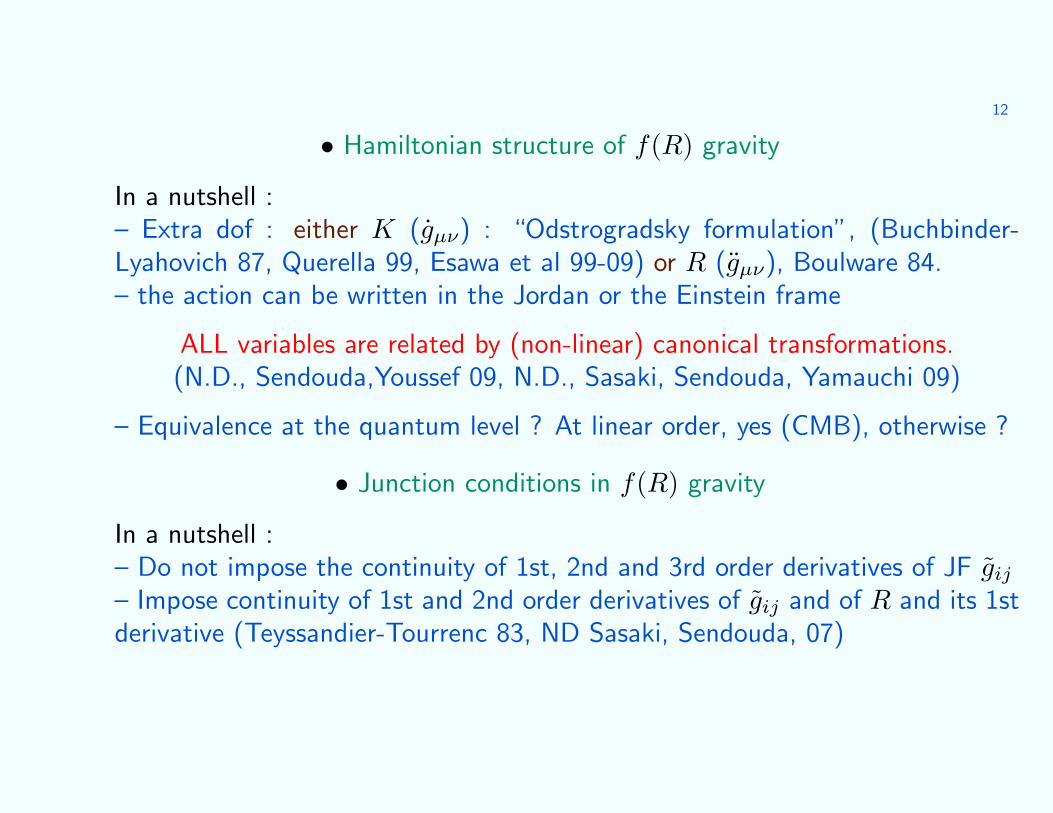
• Hamiltonian structure of f(R) gravity
In a nutshell :– Extra dof : either K (gµν) : “Odstrogradsky formulation”, (Buchbinder-Lyahovich 87, Querella 99, Esawa et al 99-09) or R (gµν), Boulware 84.– the action can be written in the Jordan or the Einstein frame
ALL variables are related by (non-linear) canonical transformations.(N.D., Sendouda,Youssef 09, N.D., Sasaki, Sendouda, Yamauchi 09)
– Equivalence at the quantum level ? At linear order, yes (CMB), otherwise ?
• Junction conditions in f(R) gravity
In a nutshell :– Do not impose the continuity of 1st, 2nd and 3rd order derivatives of JF gij
– Impose continuity of 1st and 2nd order derivatives of gij and of R and its 1stderivative (Teyssandier-Tourrenc 83, ND Sasaki, Sendouda, 07)

13
Reminder : outline of the talk
1. Introducing f(R) theories of gravity
or : f(R) theories as scalar-tensor theories of gravity
2. f(R) cosmological models of dark energyor : the search for viable models
3. f(R) gravity and local testsor : how to hide the scalar d.o.f. of gravity
4. Back to cosmological modelsor : how to hide the scalar d.o.f. of gravity
5. Remarks on Black Holes in f(R) theories
(uniqueness and thermodynamics)

14
2. f(R) cosmological models of Dark Energy
• The Carroll-Duvvuri-Trodden-Turnerand Capozziello-Carloni-Troisi proposal (2003)
f(R) = R− µ2(1+n)
Rn (n > 0) ; µ2 ∼ 10−33eV or µ2 = 1`2
with ` ∼ H−10
Late time Einstein frame Friedmann equations when matter has becomenegligible (ϕ large, > 2, say) :
3H2∗ − ϕ2 − 2V (ϕ) ≈ 0, ϕ + 3H2
∗ϕ + dVdϕ ≈ 0 with V (ϕ) ∝ e
− (n+2)ϕ
2√
3(n+1)
Solution : a∗(t) ∝ tq (q → 3 , w∗DE → −0.77 for large n), ϕ ∼√
3 p ln t
Jordan frame scale factor : ds2 = t−2pds2∗ = −dt2 + a2(t)dx2
hence : a(t) ∝ t2
3(1+wDE)
with wDE = −1 + 2(n+2)3(n+1)(2n+1) → −1 for large n (2,3,4 is enough)
15
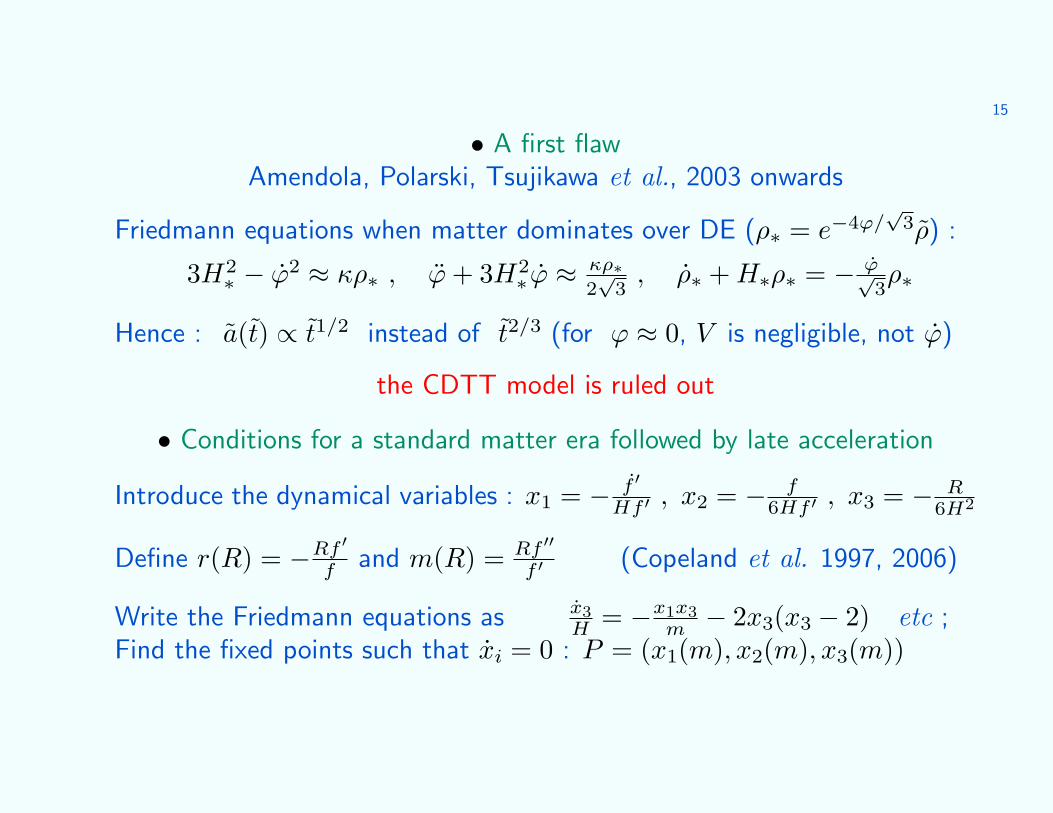
• A first flawAmendola, Polarski, Tsujikawa et al., 2003 onwards
Friedmann equations when matter dominates over DE (ρ∗ = e−4ϕ/√
3ρ) :
3H2∗ − ϕ2 ≈ κρ∗ , ϕ + 3H2
∗ϕ ≈κρ∗2√
3, ρ∗ + H∗ρ∗ = − ϕ√
3ρ∗
Hence : a(t) ∝ t1/2 instead of t2/3 (for ϕ ≈ 0, V is negligible, not ϕ)
the CDTT model is ruled out
• Conditions for a standard matter era followed by late acceleration
Introduce the dynamical variables : x1 = − f ′
Hf ′ , x2 = − f6Hf ′ , x3 = − R
6H2
Define r(R) = −Rf ′
f and m(R) = Rf ′′
f ′ (Copeland et al. 1997, 2006)
Write the Friedmann equations as x3H = −x1x3
m − 2x3(x3 − 2) etc ;Find the fixed points such that xi = 0 : P = (x1(m), x2(m), x3(m))

16
The“phase space trajectory” m = m(r) can connect a (saddle) matterpoint
PM = (r ≈ −1,m ≈ 0+) with dm/dr|−1 > −1
to a stable fixed point corresponding to
– either exponential acceleration, PS ∈ r = −2, if 0 < m(−2) ≤ 1
– or a ∝ tr, r > 1, PA ∈ m = −(1 + r), if dmdr < −1 and
√3−12 < m < 1
Example :
f(R) = R± µ2(1+n)
Rn with −1 < n < 0
Developments (Capoziello-Tsujikawa, 2007) :
– wDE < −1 for z < zb “crossing of the phantom boundary”
– wDE diverges at z = zc, zb and zc →∞ for n→ −1

17
3. f(R) gravity and local tests
• A ninety year old mistake
CDTT, 2003 : “Many solar system tests of gravity theory depend on theSchwarzschild (de Sitter) solution, which Birkhoff’s theorem ensures is theunique, static, spherically symmetric solution (...) Astrophysical tests ofgravity will be unaffected by the modification we have made.”
Weyl (1918), Pauli (1919) and Eddington (1924) had said the same...
Pechlaner-Sexl (1966), Havas (1977) : f(R) field equations are fourthorder differential equations ; they possess extra-runaway solutions : there isno Birkhoff theorem ; the solution outside an extended source is not theSchwarzschild metric and depends on its equation of state.

18
• One-scale f(R) models of DE are ω = 0 Brans-Dicke theory
Chiba (2003), Olmo (2005), Erickcek et al (2006), Navarro-Acoleyen (2006),...
The short answer :
Recall that f(R)-gravity is of Brans-Dicke type with ω = 0 and a potential
U = 12(Rf ′(R)− f(R))
Teyssandier-Tourrenc, 1983
Can U be neglected when studying gravity in the solar system ? Yes
Indeed f(R) = R−H40/R, yields U = O(H2
0) = O(1/`2) with ` LSS.
Therefore, see e.g Will or Damour-Esposito Farese, ω must be large tocomply with solar system observations : ω > 40000 (Cassini).
Hence, all one-scale f(R) models of dark energy are ruled out.

19
The details :
The equations of motion are :
D2∗ϕ−dV
dϕ = 4πG∗√3
T ∗ , G∗ij−2∂iϕ∂jϕ+g∗ij
[(∂∗ϕ)2 + 2V (ϕ)
]= 8πG∗ T ∗ij
with g∗ij = f ′gij , ρ∗ = ρ/f ′2 , f ′ = e2ϕ/√
3
Linearize : ϕ = ϕc + ϕ1, g∗ij = f ′c(ηij + hij) with Vc = O(κρc) = O(1/`2).
scalaron : 4ϕ1−m2ϕ1 ≈ −4πGeff√3
ρ (4∗ = 4/f ′c , Geff = G∗/f ′c)
m2 = f ′cd2V
dϕ2 |c = O(1/`2) whereas 4 = O(1/L2SS) hence ϕ1 ≈ GeffM√
3r
metric : ds2∗/f ′c ≈ −(1− 2GeffM/r)dt2 + (1 + 2GeffM/r)d~x2
ds2 ≈(1− 2φ1√
3
)ds2∗
f ′c≈ −
(1− 2GM
r
)dt2 +
(1 + 2γGM
r
)d~x2 , G = 4Geff
3 , γ = 1/2

20
A scalar curvature “locked” at its cosmological, small, value :
Equation of motion for the scalar curvature (or scalaron, that is, ϕ) :
3D2f ′ + (Rf ′ − 2f) = κT (not R = κT as in GR !)
Linearize : R = Rc + R1 so that D2R1 −m2R1 = κT3f ′′c
, m2 = (f ′−Rf ′′)|c3f ′′c
Solve with source being, say, a constant density star—or numerically,Multamaki-Vilja, Kanulainen et al, (2007)
and find that, if mr 1, then R ≈ Rc outside and inside the star.
**
On the other hand, if mr 1, find Schwarzschild (hence γ = 1) :
ds2 ≈ −(1− 2GM(1−ε)
r
)dt2 +
(1 + 2GM(1+ε)
r
)d~x2 , ε = e−m(r−r)
2m2r2≈ 0
but... R ≈ −κT Rc inside the star : linear approximation breaks down

21
• Where do we stand ?
– the original CDTT model f(R) = H20(RH−2
0 − 1/(RH−20 )n) failed :
final acceleration but no matter era
– various one-scale cosmologically viable models had been proposed, e.g. :f(R) = H2
0(RH−20 + (RH−2
0 )n) with 0 < n < 1
– all badly failed to comply with local gravity constraints because the scalarcurvature is locked at its cosmological value R = O(H2
0) = O(κρcosmo)everywhere, even inside the Sun where, instead, GR gives R = O(κρ)
– however, if the scalaron could be given a heavy mass, the linearapproximation (violated in that limit) indicates that the gravity field of theSun would be the same as in GR
– hence : look for two-scale f(R) models and solve the full non-linearscalaron eom

22
• Conventional wisdom...:e.g. Starobinski, 2007
linearise the scalaron eom on the SS background : dVdϕ |SS ∝ κρ :
4ϕ1 −m2ϕ1 ≈ 0 with m2 = f ′−Rf ′′
3f ′′
If, for R 1/`2, e.g. R ∼ κρ : f ′ → 1 and m2SS ≈ 1
3f ′′|SSis positive and
large ((mL)SS 1) then deviations from Einstein’s GR are small.
CDTT model : m2SS is large and negative (Dolgov-Kawasaki, 2003)
• ...and the “Chameleon” effectKhoury-Weltman (2003)
Navarro-Acoleyen (2006), Capozziello-Tsujikawa (2007)
or : how can the scalar curvature become equal to the local matter density

23
Chameleon details (Takami-Tsujikawa 2008)
(For a review see Brax et al., P. Brax ihes seminar)
Once again, look at scalaron eom : D2∗ϕ− dV
dϕ = κ2√
3T∗
In ≈ flat background : 4∗ϕ = dVeffdϕ with dVeff
dϕ = dVdϕ −
κρ∗2√
3
Contrarily to V , Veff may have minima for ϕ = ϕ inside the Sun and forϕ = ϕe outside. One looks for ϕ|e, = ϕ(Re,) such that Re, ≈ κρe,.
Solution outside : ϕ = ϕe + C rr when mer 1 with m2
e = d2Vdϕ2 |e
Solution inside : ϕ ≈ ϕ up to r = r1, then interpolation to ϕ outside.
if r1 ≈ r, then C = 3βClin with β = ϕe−ϕGM/r
≈ ϕeGM/r
One needs β < 10−5 to have γ − 1 < 10−5 (Cassini)

24
• A new family of f(R) models of dark energy
Hu-Sawicki (2007), Starobinski (2007), Odintsov et al (2008), ...
f(R) = R + λRc
[1
(1+R2/R2c)
n − 1], etc
dVdϕ −
κρe
2√
3= 0 gives ϕe = O (ρc/ρe)
2n+1
Now, β ≈ ϕeGM/r
≈ 106ϕe < 10−5 ; hence ϕe < 10−11
For ρe = ρgalaxy = 105ρc then ϕe = O(10−5(2n+1)) and hence themodels evade Local Gravity Constraints as soon as n > 1/2
In a nutshell : the Chameleon effect relies on (1)“locking” ϕ, that is, thescalar curvature, on its Einstein value inside the Sun, and (2) on a localenvironment much denser than the asymptotic, cosmological, value.
• Beyond flat background : f(R) dense star models
Frolov (2008); Kobayashi-Maeda (2008) : Rcentral →∞ ?Babichev-Langlois (2009) : NO, if ρ− 3P > 0.

25
4. Back to cosmology : “cured viable” models
• An uncontrolable scalaron instability ?
The new family of models yield cosmological scale factors which areundistinguishable from Λ-CDM until after the end of the matter era andtend to a de Sitter regime a ∝ eHt.... However, because the mass of the scalaron is chosen to be high inhigh matter density environment (in order to comply with Local gravityConstraints), the cosmological perturbations of the scalaron diverge inthe early matter era unless their amplitude is tuned to a very small value.
Starobinski (2007), Tsujikawa (2007)... but this problem can be cured too :
f(R) = R− µRc(R/Rc)
2n
(R/Rc)2n+1+ R2
6M2
Appleby, Battye and Starobinsky (2009).............. Better than Λ ???

26
• f(R) models of Dark Energy, summary– Failed attempt ? technically no, observationaly, not yet...
— ...aesthetically... ?

27
... What is then the origin of the present acceleration of the universe ?...
• “Modified” gravity ?– f(R)-gravity : standard models : not convincing ; “detuned” f(R)?– MOND ? “Branes” ?
• Exotic matter ?– Chaplygin gas ? Quintessence ? (see Efstathiou et al. 2007)
• An artefact of the averaging process ?Gij(<gkl>) = κ <Tij > instead of <Gij(gkl)>= κ <Tij >
• ... or “simply” Λ ?usual objections : why so small, and why now ? Bianchi-Rovelli (2010) :
– Λ is no “blunder”– no strong probability argument against “now”– if 120 orders of magnitude off HEP prediction: HEP problem !

28
Reminder : outline of the talk
1. Introducing f(R) theories of gravity
or : f(R) theories as scalar-tensor theories of gravity
2. f(R) cosmological models of dark energyor : the search for viable models
3. f(R) gravity and local testsor : how to hide the scalar d.o.f. of gravity
4. Back to cosmological modelsor : how to hide the scalar d.o.f. of gravity
5. Remarks on Black Holes in f(R) theories
(uniqueness and thermodynamics)
29
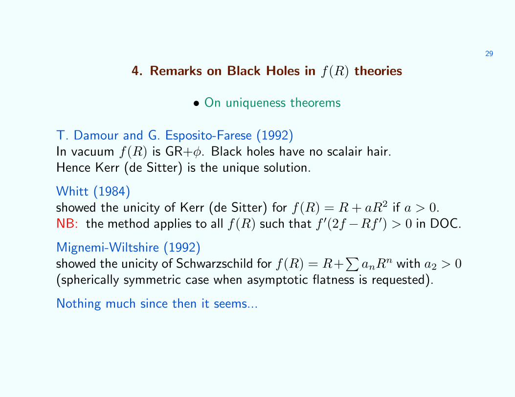
4. Remarks on Black Holes in f(R) theories
• On uniqueness theorems
T. Damour and G. Esposito-Farese (1992)In vacuum f(R) is GR+φ. Black holes have no scalair hair.Hence Kerr (de Sitter) is the unique solution.
Whitt (1984)showed the unicity of Kerr (de Sitter) for f(R) = R + aR2 if a > 0.NB: the method applies to all f(R) such that f ′(2f−Rf ′) > 0 in DOC.
Mignemi-Wiltshire (1992)showed the unicity of Schwarzschild for f(R) = R+
∑anRn with a2 > 0
(spherically symmetric case when asymptotic flatness is requested).
Nothing much since then it seems...
30
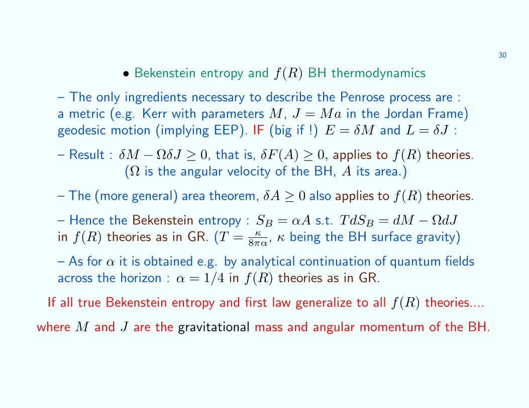
• Bekenstein entropy and f(R) BH thermodynamics
– The only ingredients necessary to describe the Penrose process are :a metric (e.g. Kerr with parameters M , J = Ma in the Jordan Frame)geodesic motion (implying EEP). IF (big if !) E = δM and L = δJ :
– Result : δM −ΩδJ ≥ 0, that is, δF (A) ≥ 0, applies to f(R) theories.(Ω is the angular velocity of the BH, A its area.)
– The (more general) area theorem, δA ≥ 0 also applies to f(R) theories.
– Hence the Bekenstein entropy : SB = αA s.t. TdSB = dM − ΩdJin f(R) theories as in GR. (T = κ
8πα, κ being the BH surface gravity)
– As for α it is obtained e.g. by analytical continuation of quantum fieldsacross the horizon : α = 1/4 in f(R) theories as in GR.
If all true Bekenstein entropy and first law generalize to all f(R) theories....
where M and J are the gravitational mass and angular momentum of the BH.

31
• Wald entropy and “Global charges” of f(R) spacetimes
Entropy as a Noether charge, Wald (1993) : SW = f ′(Rh)S.
Various methods to define global charges : Euclidean methods plus :
– Start with eg Kerr (M , a, Jordan Frame). Go to the Einstein frame(where no geodesic motion) : at∞, M →
√f ′∞M , ξt =
√f ′∞(1, 0, 0, 0).
Obtain the global charges as Mi = f ′∞M , Ji = f ′∞J .
– Hamiltonian formulation (ADM, 1959)Vary f(R) action with a YGH term in JF, keep track of boundary terms
S = 12κ
∫d4x√−g [f ′(s)R− (sf ′(s)− f(s)] + 1
κ
∫∂V d3x
√|h|K f ′(s)
Obtain :EADM ≡ Hon shell = −1
κ
∫S d2x
√σ(f ′(s)k + f ′′ra∂as) = f ′∞M
NB : OK with Deser-Tekin (2002), not Deser-Tekin (2007)
– Ashtekar-Magnon (1984) method (see also, ND, J Katz, 2006)applied to f(R) in JF yields Mconf = f ′∞M (Koga et al, 2005).

32
begin(• The Katz Bicak Lynden-Bell method (1985, 1997)
– Nœther identities, conserved current, superpotential and charge :Vary L ≡
√−g L + surface term for xµ → xµ + ξµ ; get (on shell) :
∂µjµ = 0 =⇒ ∂µj[µν] = jν
=⇒ q ≡∫
SdD−2x j[01] is constant in time.
– Choice for the vector ξµ :
Translation (mass) and rotation (angular momenta) Killing vectors,“appropriately” normalized
– Regularization (“zero point energy”, background) :
Q ≡∫
SdD−2J [01] ; J [µν] ≡ − 1
16π(j[µν] − j[µν])– Choice for surface term :
L ≡ L + Dµkµ where the vector kµ is chosen “appropriately”
– Extensions : ND-Katz-Ogushi (03) ; ND-Katz (04); ND-Morisawa (05)

33
• KBL mass in f(R) theories (ND, 2007)
δ∫M dDx (L + Dµkµ) =
∫∂M dD−1x nµ(V µ + δkµ) (on shell)
with L = f(R) and V µ = −(⊗µνρδgνρ −⊗µνρσ δΓσ
νρ)
δgµν = 2D(µξν), find : j[µν] = 2(2ξ[µDν]f ′(R) + Dµ[ξν]f ′(R) + ξ[µkν])
choose kµ = (gµν∆ρνρ − gνρ∆µ
νρ)f′(R) where ∆µ
νρ ≡ Γµνρ − Γµ
νρ
Hence Q = − 18π
∫S∞
dD−2x(D[0ξ1] −D[0ξ1] + ξ[0k1]
)(”Komar +”).
choose ξµ : timelike KV ξµ = (1, 0, 0, 0)
find, for Kerr (de Sitter) solution : Mi = f ′(R∞)M
Note that for purely quadratic theories : f ′(R∞) = f ′(0) = 0...(Deser-Tekin 2007)
end)
34
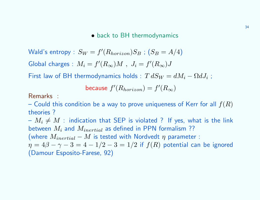
• back to BH thermodynamics
Wald’s entropy : SW = f ′(Rhorizon)SB ; (SB = A/4)
Global charges : Mi = f ′(R∞)M , Ji = f ′(R∞)J
First law of BH thermodynamics holds : T dSW = dMi − ΩdJi ;
because f ′(Rhorizon) = f ′(R∞)Remarks :– Could this condition be a way to prove uniqueness of Kerr for all f(R)theories ?– Mi 6= M : indication that SEP is violated ? If yes, what is the linkbetween Mi and Minertial as defined in PPN formalism ??(where Minertial −M is tested with Nordvedt η parameter :η = 4β − γ − 3 = 4 − 1/2 − 3 = 1/2 if f(R) potential can be ignored(Damour Esposito-Farese, 92)

35
When question marks begin to accumulate it is wiser to stop...
Thank you for your attention