topics in labor economics - uni- · pdf fileprof. bernd fitzenberger, ph.d. ws 2013/2014...
TRANSCRIPT

Prof. Bernd Fitzenberger, Ph.D. WS 2013/2014
Topics in Labor Economics
Content: This lecture is a topics course covering current research issues in laboreconomics. Prerequisites include basis microeconomic theory, intermediate eco-nometrics and the lecture ’Labor Economics for Master/Diploma’ or equivalentprior knowledge. The course has two parts. In the first part, there is a series offive lectures on static and dynamic labour supply models, human capital, labordemand, and search and matching theory. In the second part, participants willhave to present and discuss critically a research paper or a policy report and towrite a critical referee report on the chosen paper/report. The referee report hasto be turned in on the day of the presentation. A particular emphasis in this courseis on the interaction of theoretical and empirical modelling and its relevance foreconomic policy. The students in the course will learn to understand and criticallydiscuss current research papers and reports in the area of labor economics. It isrecommended for students to have a good background in economic theory andeconometrics.
The assignment of the research papers to be discussed by the students take placeduring the first and second lecture.
Time Schedule
Five Lectures
1. Labor Supply (Thursday November 7, 10:00h – 14:00h)
2. Human Capital (Thursday November 14, 12:00h – 14:00h)
3. Labor Demand (Thursday November 28, 10:15h – 12:30h)
4. Search and Matching Theory (Thursday December 19, 10:30h – 14:00h)
The presentations of the research papers will take place on:
1. Wednesday 29 January 2013: 14:00-18:00h
2. Thursday 30 January 2013: 10:00-14:00h
1

All lectures and paper presentations take place in room 2330 (KG II).
References:
• O. Ashenfelter and D. Card (eds) (1999) Handbook of Labor Economics,Volume 3A-C, North-Holland.
• O. Ashenfelter and D. Card (eds) (2011). Handbook of Labor Economics,Volume 4A and 4B, North Holland, Elsevier, Amsterdamm.
• P. Cahuc and A. Zylberberg (2004) Labor Economics. MIT Press, Cam-bridge, Massachusetts.
• Franz, W. (2013) Arbeitsmarktokonomik. 8th edition, Springer.
Section 1: Read the chapter by Blundell/MaCurdy in Ashenfelter/Card (1999)and Franz (2009, chapter 2)
Section 2: Read the chapter by Card in Ashenfelter/Card (1999) and Franz (2009,chapter 3)
Section 3: Read Franz (2009, chapter 4) and Cahuc/Zylberberg (2004, chapter4)as well as- Acemoglu, D. (2002), Technical Change, Inequality and the Labor Market.Journal of Economic Literature.- The chapter by Autor and Acemoglu in Ashenfelter/Card (2011)
Section 4: Read Cahuc/Zylberberg (2004, chapter 3)as well as- The chapter by Mortensen and Pissaridis in Ashenfelter/Card (1999)
2
Course Material – Section 1. Labor Supply
• Participation
• Home production
• Family labor supply
Dimensions of Labor Supply
- Quantity dimension: Number of persons supplying labor (head count)
- Behavioral dimension: Participation, hours
- Quality dimension: Heterogeneity in ability and education
Measures:
Participation rate =
EMP
Employees +UNP
Unemployed PersonsPopulation [in working age]
POP
Employment rate =Employees
Population [in working age]
Unemployment rate =Unemployed persons
EMP + UNP
Labor Supply = EMP + UNP ?
3
Static Models of Labor Supply
Reservation Wage versus Market Wage
Individual i:
- Reservation wage wRi
- Market wage wi
Individual i will offer Hi hours of work, if wi ≥ wRi
Formally this means
Hi
{= 0 for wi ≤ wR
i
> 0 wi > wRi
wi and wRi are determined by:
wi = XMi · β =km∑j=1
XMi,j · βj(1)
wRi = XRi · βR =
kR∑j=1
XRi,j · βRj(2)
where XMi , XRi are determinants of wi, wRi (row vectors) and β, βR are
column vectors of coefficients (magnitude of the influence), respectivelyThen, the decision rule can be written as:
Hi
{= 0 for XMi · β ≤ XRi · βR
> 0 XMi · β > XRi · βR
Assumption here: wi is exogenously predeterminedThis assumption will be given up later
→ Investments in Human Capital→ Search Theory
Here, we discuss the factors that influence wRi : opportunity costs of work
→ The value of leisure time→ Other income→ Situation in family
4

Participation and the Hours of Work as a Result of Individual UtilityMaximization
- The labor supply is derived from the demand of leisure time as part ofindividual utility maximization problem → Consumer demand frommicroeconomics
Utility function:
U = U(X,F,R, µ)
X: consumption of goodsF: leisure timeR: observable individual characteristicsµ: unobservable individual characteristics
Assumption: U is quasi-concave and twice differentiable
UX =∂U
∂X> 0, UF =
∂U
∂F> 0, UXX =
∂2U
∂X2< 0, UFF =
∂2U
∂F 2< 0
- Positive but diminishing marginal utility
Constraints:
F = T −H T: Total disposable hoursH: Hours of work
F ≥ 0H ≥ 0
PX = W ·H + V P: Price of consumption good (assumptionof a representative good)V: Non-labor income
X ≥ 0
One can restrict analysis to the following two cases:
H > 0 ParticipationH = 0 No participation
5

Kuhn–Tucker Problem
max U(X,T −H)s.t. PX = wH + VH ≥ 0
Lagrange Function:
L = U(X,T −H︸ ︷︷ ︸F
)− λ(PX − wH − V ) + κH; κ > 0 for H = 0
κ = 0 for H > 0
First Order Conditions:
(1) ∂L∂X = UX − λP = 0
(2) ∂L∂H = −UF + λw = 0 for H > 0
≤ 0 for H = 0
6
-
κ > 0
H
H = 0L
0
6

Approach : U is quasi-concave
1) Solve (1)+ (2) for X and H→ If solution results in X,H > 0, then there exists interior solution andindividual supplies work.
2) Solve (1) for H = 0→If there is no solution under (1), then this is the solution.
Interior solution, H > 0:
It follows from (1)+(2) that
UX = λPUF = λw
} UFUX
= wP
↑ ↑Marginal rate of substitution Real wage
H=0:
UFUX≥ w
p
i.e. if the marginal utility from leisure time relative to the marginal utility fromconsumption exceeds the real wage at zero hours already, then the individualdoesn’t supply any labor.
The other way round, the marginal utility ratio at zero hours defines the realreservation wage, i.e. the minimal level of wage for a positive labor supply.
wR
P=UF
UX
∣∣∣∣∣H=0
or wR = P · UF
UX
∣∣∣∣∣H=0
7
Graphical Analysis
6
-
PPPPPPPPPPPPPPPPPP
I1
I2
F1 T
T − F1 = H1
F(Leisure)
VP
X1
wT+VP
X(Consumption)
Budget line with the slope− wP
����
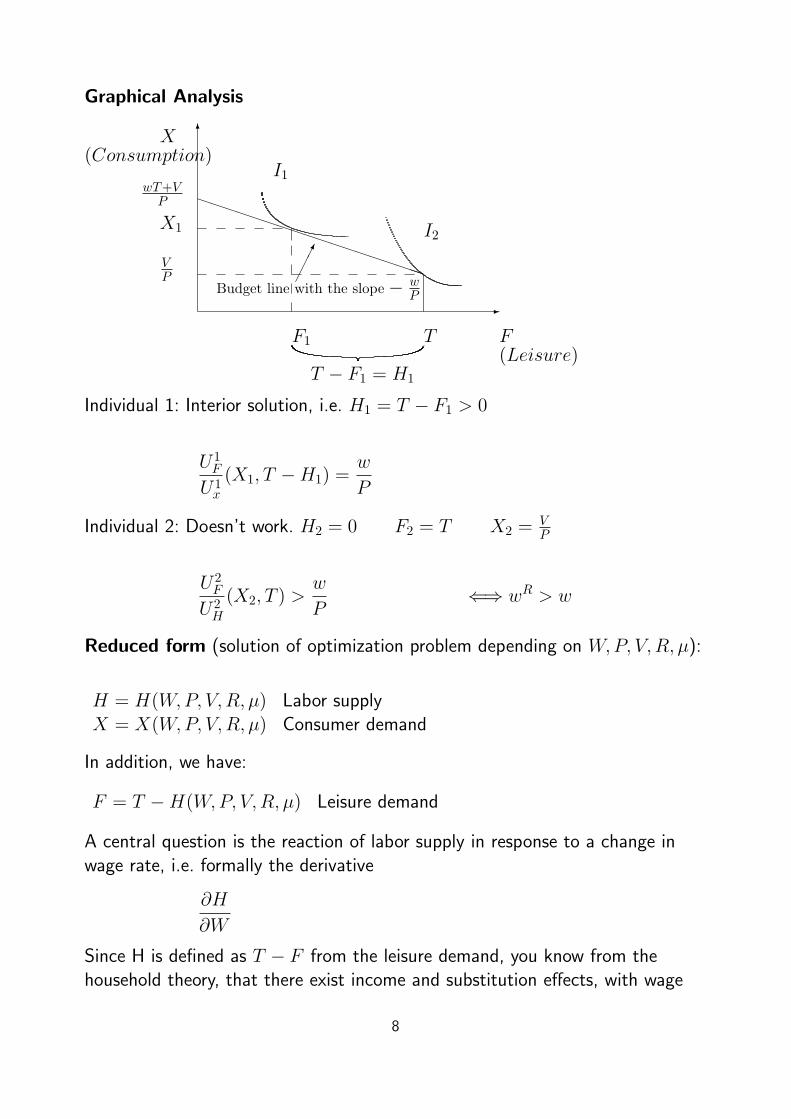
Individual 1: Interior solution, i.e. H1 = T − F1 > 0
U 1F
U1x
(X1, T −H1) =w
P
Individual 2: Doesn’t work. H2 = 0 F2 = T X2 =VP
U 2F
U 2H
(X2, T ) >w
P⇐⇒ wR > w
Reduced form (solution of optimization problem depending on W,P, V,R, µ):
H = H(W,P, V,R, µ) Labor supplyX = X(W,P, V,R, µ) Consumer demand
In addition, we have:
F = T −H(W,P, V,R, µ) Leisure demand
A central question is the reaction of labor supply in response to a change inwage rate, i.e. formally the derivative
∂H
∂W
Since H is defined as T − F from the leisure demand, you know from thehousehold theory, that there exist income and substitution effects, with wage
8
being the price for leisure. For the interior solution (H > 0), this is shown bythe Slutsky decomposition:
∂H
∂w=
(H∂H
∂V
)︸ ︷︷ ︸
Income effect (-)
+
(∂H
∂w
)s︸ ︷︷ ︸
Substitution effect (+)
⇓here ∂F
∂V > 0 if leisure is not an inferior good
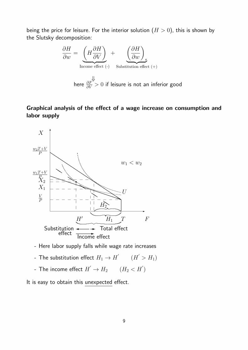
Graphical analysis of the effect of a wage increase on consumption andlabor supply
6
-
r
H1
H2
w1 < w2
Income effect
Substitutioneffect
Total effect� -
PPPPPPPPPPPPPPPPPP
-
QQQ
QQQQ
QQQ
QQQQ
QQQQ
X
F
X1
X2
w1T+VP
w2T+VP
VP
H ′ T
U
- Here labor supply falls while wage rate increases
- The substitution effect H1 → H′
(H′> H1)
- The income effect H′ → H2 (H2 < H
′)
It is easy to obtain this unexpected effect.
9
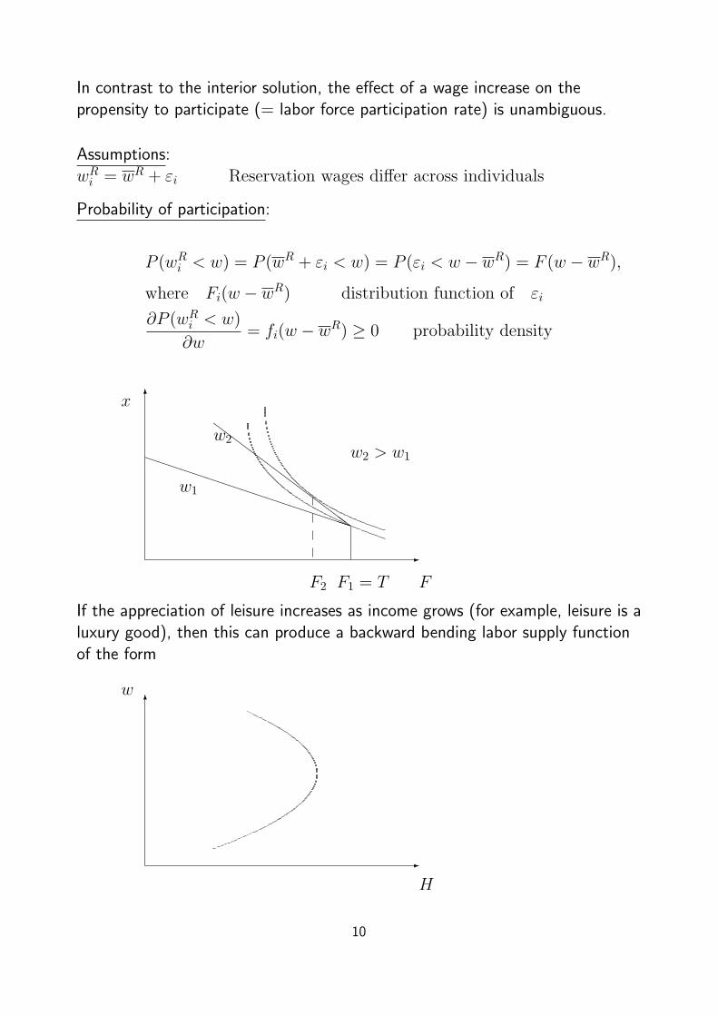
In contrast to the interior solution, the effect of a wage increase on thepropensity to participate (= labor force participation rate) is unambiguous.
Assumptions:wR
i = wR + εi Reservation wages differ across individuals
Probability of participation:
P (wRi < w) = P (wR + εi < w) = P (εi < w − wR) = F (w − wR),
where Fi(w − wR) distribution function of εi
∂P (wRi < w)
∂w= fi(w − wR) ≥ 0 probability density
6
-
PPPPPPPPPPPPPPPPPP
x
F
ZZ
ZZZ
ZZZZ
ZZZ
w1
w2
F2 F1 = T
w2 > w1
If the appreciation of leisure increases as income grows (for example, leisure is aluxury good), then this can produce a backward bending labor supply functionof the form
6
-
w
H
10
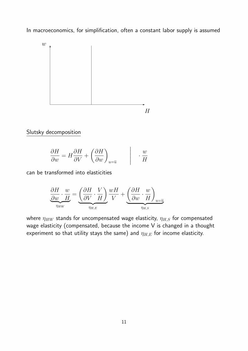
In macroeconomics, for simplification, often a constant labor supply is assumed
6
-
w
H
Slutsky decomposition
∂H
∂w= H
∂H
∂V+
(∂H
∂w
)u=u
∣∣∣∣∣ · wH
can be transformed into elasticities
∂H
∂w· wH︸ ︷︷ ︸
ηHW
=
(∂H
∂V· VH
)︸ ︷︷ ︸
ηH,E
wH
V+
(∂H
∂w· wH
)u=u︸ ︷︷ ︸
ηH,S
where ηHW stands for uncompensated wage elasticity, ηH,S for compensatedwage elasticity (compensated, because the income V is changed in a thoughtexperiment so that utility stays the same) and ηH,E for income elasticity.
11

Slutzky Decomposition for Interior Solution
(S)∂H(w, V )
∂W= H
∂H
∂V︸ ︷︷ ︸Income effect
+
(∂H
∂W
)s︸ ︷︷ ︸
Substitution effect
where w hourly wage, V nonlabor income, and H(w, V ) Marshallian labor supply (based ondemand for leisure).
Substitution effect: ( ∂H∂W
)s > 0
Income effect: ∂F∂V
> 0 assuming leisure is a normal good ⇔ ∂H∂V
< 0Therefore sign of ∂H
∂Wis ambiguous
Note: If leisure is an inferior good (∂F/∂V < 0⇔ ∂H/∂V > 0), then unambiguously it holds∂H/∂W > 0 .
We show the comparative static result (S):
First order conditions for interior solution
(1a) UF − λw = 0(1b) Ux − λp = 0
}(1) pUF−wUx = 0
(2) px− wH = V
→ Total differentiation of (1) and (2) with respect to x,H (these are the endogenous variables)and w, V (these are the exogenous variables), respectively
Differentiate with respect to x,H, and w:
(1′) −pUFFdH + pUFxdx− UxdW + wUxFdH − wUxxdx = 0
(2′) pdx−HdW − wdH = 0
In matrix notation:(−pUFF + wUxF pUFx − wUxx
−w p
)(dHdx
)=
(Ux
H
)dW
By Cramer´s rule, we have:
dH
dW=
∣∣∣∣ Ux pUFx − wUxx
H p
∣∣∣∣∣∣∣∣ −pUFF + wUxF pUFx − wUxx
−w p
∣∣∣∣ =+︷︸︸︷pUx −Hp
?︷︸︸︷UFx +wH
−︷︸︸︷Uxx
D︸︷︷︸+
→ sign of dH/dW is ambiguous
Sign of denominator D :
D = −p2UFF + wpUxF + wpUFx − w2Uxx
= −(pw)(UFF UFx
UxF Uxx
)(wp
)> 0
12
since middle matrix is negative definite.
Now, it is necessary to determine the income effect: Total differentiation
(−pUFF + wUxF pUFx − wUxx
−w p
)(dHdx
)=
(01
)dV
dH
dV=
∣∣∣∣ 0 pUFx − wUxx
1 p
∣∣∣∣D
=−
?︷ ︸︸ ︷pUFx +
−︷ ︸︸ ︷wUxx
D︸︷︷︸+
?
UFx is presumably positive → Marginal utility of consumption increases with leisure
Leisure is no inferior good:
dH
dV< 0 ⇔ dF
dV> 0 since dF = −dH
Substitution effect:
(1′) (−pUFF + wUxF )dH + (pUFx − wUxxdx = UxdW
and individual stays on a given indifference curve
(3) dU = −UFdH + Uxdx = 0
Solution by Cramer’s rule:
(dH
dW
)s
=
∣∣∣∣ Ux pUFx − wUxx
0 Ux
∣∣∣∣Ux(−pUFF + wUxF ) + UF (pUFx − wUxx)
=pUx
−p2UFF + wpUxF + UF
Ux· (p2UFx − wpUxx)
First order condition: UF
Ux= w
p(dH
dW
)s
=pUx
−p2UFF + wpUxF + wpUFx − w2Uxx
=pUx
D> 0
Thus, Slutzky decomposition follows:
dH
dW=pUx
D+H
wUxx − pUFx
D=
(dH
dW
)s
+HdH
dV
... and the derivation is completed!
13
Taxation of Labor Income: Less Clear Effects
Linear income tax
w · (1− t)︸ ︷︷ ︸w
H + V (t) = P ·X (t: tax rate)
w: net wage (analysis as above)
∂H
∂t=∂H
∂w· ∂w∂t
+∂H
∂V· dVdt
=
[(∂H
∂w
)s
+H
(∂H
∂V
)](−w) + ∂H
∂V· dVdt
ambiguous +
> 0 if income effect dominates< 0 if substitution effect dominates
+ − − −−−
⇒ As long as leisure is not an inferior good, also tax effect is ambiguous.
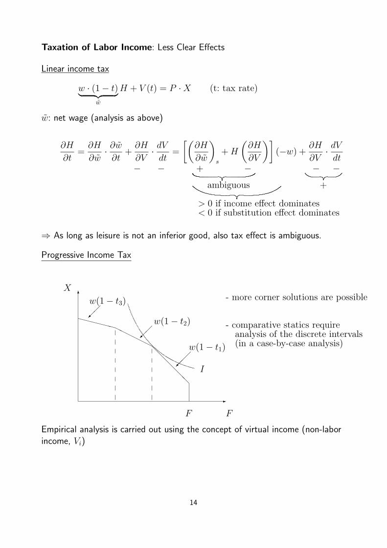
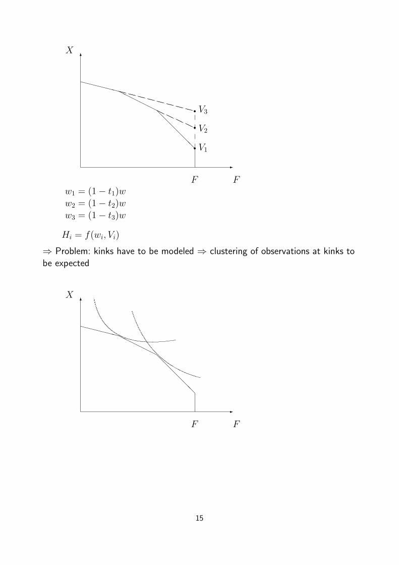
Progressive Income Tax
6
-
F
X
F
w(1− t1)
w(1− t2)
w(1− t3)
���
��
��
I
@@@@
@@
HHHHHH
XXXXXX
- more corner solutions are possible
- comparative statics requireanalysis of the discrete intervals(in a case-by-case analysis)
Empirical analysis is carried out using the concept of virtual income (non-laborincome, Vi)
14
HH HH HH HH
XX XX XX XX XX XX XX XX
rrr
6
-
@@@@
@@
HHHHHH
XXXXXX
F
X
F
V1
V2
V3
w1 = (1− t1)ww2 = (1− t2)ww3 = (1− t3)w
Hi = f(wi, Vi)
⇒ Problem: kinks have to be modeled ⇒ clustering of observations at kinks tobe expected
6
-
@@@@
@@
HHHHHH
XXXXXX
F
X
F
15

Non-convex budget constraint due to a high tax rate for welfare transfers(benefit withdrawal rate):
6
-
hhhhhaa
ll
llll
HHH
XXX
r rrrr
r
F
x
Cases to be distinguished: comparison of optimal interior/corner solutions innon-convex part
• Hours H are not a continuous function of wage rate
• Observations clustering at the kink points is not observed in actual data
⇒ Differentiable Approximation of the Budget Constraint: MaCurdy etal.(1990)
16
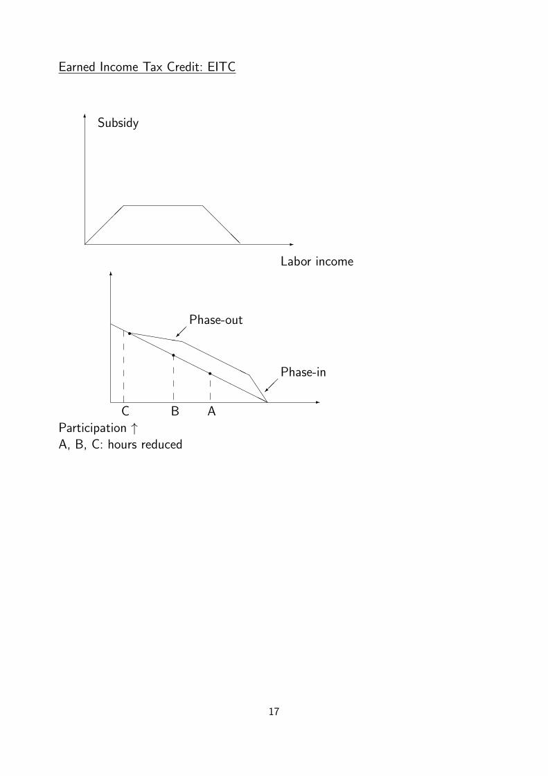
Earned Income Tax Credit: EITC
6
-
Subsidy
Labor income
����� @
@@@@
6
-
rrrHHHHHHHHHHHHHHHHHH
ABC
hhhhhhHHHHHHHH
JJ
J
Phase-out
Phase-in
��
��
Participation ↑A, B, C: hours reduced
17

Home Production
6
-
��������
PX
HHHHHHHHHHHHHHHHHH
T
f(h2)
wh1
h1: time in paid job
h2: time in home production
P=1
max U(
F︷ ︸︸ ︷T − h1 − h2, X)
s.t. X = f(h2) + wh1
L = U(F,X)−λ[X − f(h2)− wh1]
(1) ∂U∂h1
= −UF + λw = 0 Interior solution
(2) ∂U∂h2
= −UF + λf ′(h2) = 0
(3) ∂U∂X = Ux − λ = 0 ⇔ λ = UX
(1′) UF = UXw
(2′) UF = UXf′(h2)
}f ′(h2) = w → h∗2(w)
6
-
X
FTh∗2h∗1
Interior solutionbbbb
bbbb
bbrr
18

6
-
X
FT
bbbb
bbbb
bbr
T -h2 T -h∗2
h∗1 = 0
19

Intertemporal Labor Supply
max{x(t),F (t)}
V (0) =
K∑t=0
(1 + s)−tU [x(t), F (t)]
s.t.:A(0) +K∑t=0
(1 + r)−t[w(t)H(t)− P (t)x(t)] = 0
T = H(t) + F (t)
Lagrangean
L = V (0) + λ{A(0) +k∑t=0
(1 + r)−t[w(t) ·H(t)− P (t)x(t)]}
First order conditions:
(i) (1 + s)−tUx(t)− λ(1 + r)−tP (t) = 0
(ii) (1 + s)−tUF (t)− λ(1 + r)−tw(t) ≥ 0
(iii) A(0) +∑k
t=0(1 + r)−t[w(t) ·H(t)− P (t)x(t)] = 0
Reduced form solutions (interior solution for i + ii)
H(t) = H [λθtw(t), λθtP (t)]
x(t) = x[λθtw(t), λθtP (t)]
with θ = 1+s1+r given λ Frisch demand.
20

w(t), wR(t)
Ag
w1(t) = w0(t) + w
���
wR1 (t)
wR0 (t)
t1 t2 t3 t4 t5 t6 t7 t8 K
w0(t)
���
w0(t)→ w1(t)
wR1 (t) > wR
0 (t)
• Working life reduced form t3 − t8 to t4 − t7• Works more hours during [t5, t6]
• Works less hours during [t4, t5] + [t6, t7]
21

Empirical Specification of Participation Probability using a Probit Model
Ii =
{1 for wi > wR
i : Hi > 0
0 for wi ≤ wRi : Hi = 0
EIi = Pr(wi > wRi ) · 1 + Pr(wi ≤ wR
i ) · 0= Pr(wi > wR
i )
= Prob. of Participation
Probit Model assumes:
EIi = Pr(Hi > 0) = Φ(xiβ) = Φ
(n∑k=0
xikβk
)with Φ(z) distribution function of standard normal
xi1, ..., xin factors affecting participation
φ(z) =dΦ(z)
dz=
1√2πe−
z2
2 density of a standard normal
Effect of xik on participation probability
∂Pr(Hi > 0)
∂xik= βkφ(
n∑k=1
xikβk) = βkφ(xiβ)
Maximum Likelihood Estimation
maxβL =
N1∏i=1
Φ(xiβ)︸ ︷︷ ︸Hi > 0 for i = 1, .., N1
·n∏
i=N1+1
[1− Φ(xiβ)]︸ ︷︷ ︸Hi = 0 for i = N1 + 1, .., N
22

Problem of Sample Selection Bias
wi only observable when Hi > 0 : Ii = 1
wi typically not known when Hi = 0 : Ii = 0
Estimation of coefficients γ in
wi = XMiγ + vi i = 1, ..., N1
is biased because based only on employees.
Employed : Ii = 1
with E[vi|Ii = 1, xi] = δ ·M(xiβ)
joint normality = δ · φ(xiβ)Φ(xiβ)
= 0
M(xiβ) is called the inverse Mills Ratio
Consistent estimation with selection correction term (Heckman
Correction) wi = XMiγ + δM(xiβ) + vi based on estimated β.
⇒ yields consistent estimates for γ and δ.
Problem Endogeneity of Market Wage
wi = XMiγ + vi Wage equation(4)
Hi = αwi + xiθ + εi Hours equation if hours positive(5)
Correlation between error terms vi and εi implies that equation (5)
cannot be estimated consistently, i.e. α and θ cannot be determined
consistently.
Endogeneity of wi as explanatory variable in the hours equation.
23
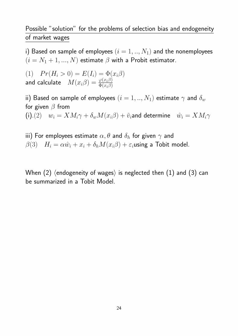
Possible ”solution” for the problems of selection bias and endogeneity
of market wages
i) Based on sample of employees (i = 1, .., N1) and the nonemployees
(i = N1 + 1, ..., N) estimate β with a Probit estimator.
(1) Pr(Hi > 0) = E(Ii) = Φ(xiβ)
and calculate M(xiβ) =φ(xiβ)Φ(xiβ)
ii) Based on sample of employees (i = 1, .., N1) estimate γ and δwfor given β from
(i).(2) wi = XMiγ + δwM(xiβ) + viand determine wi = XMiγ
iii) For employees estimate α, θ and δh for given γ and
β(3) Hi = αwi + xi + δhM(xiβ) + εiusing a Tobit model.
When (2) ⟨endogeneity of wages⟩ is neglected then (1) and (3) can
be summarized in a Tobit Model.
24
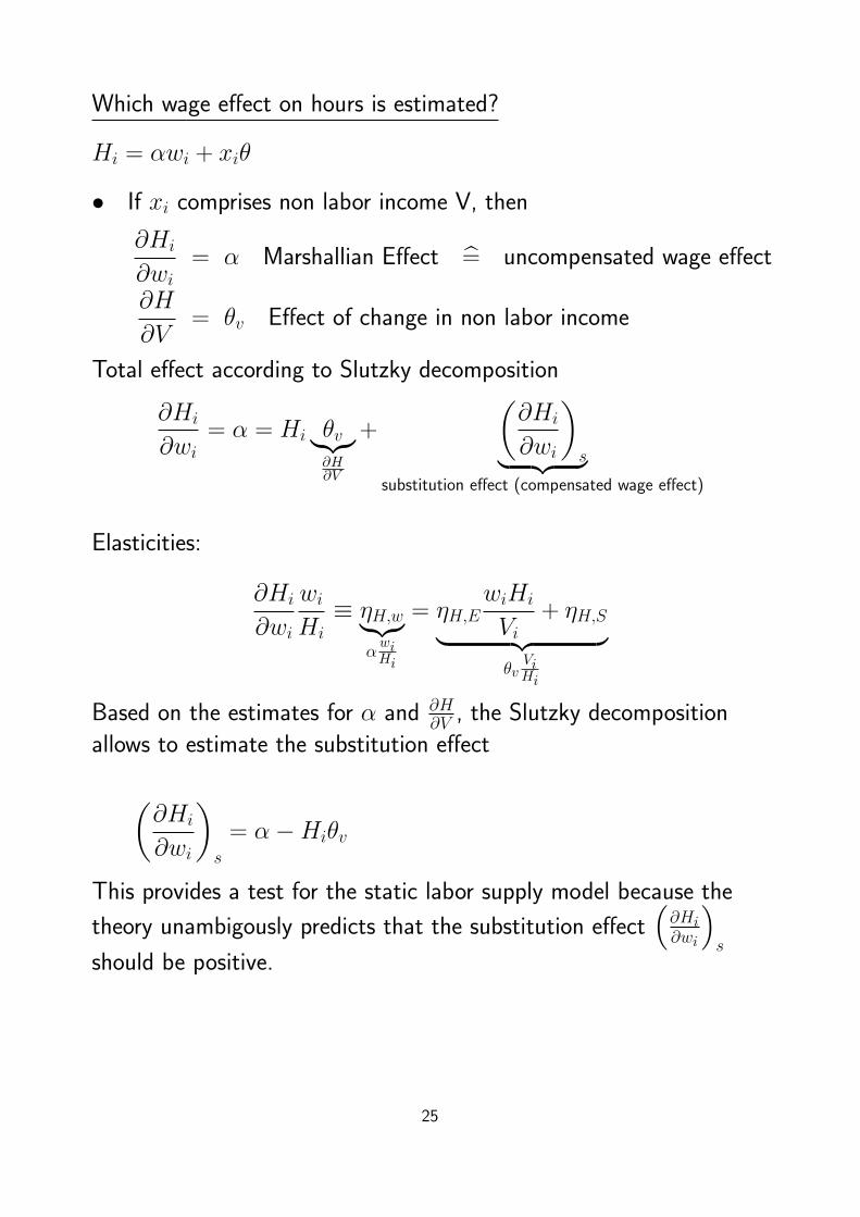
Which wage effect on hours is estimated?
Hi = αwi + xiθ
• If xi comprises non labor income V, then
∂Hi
∂wi= α Marshallian Effect = uncompensated wage effect
∂H
∂V= θv Effect of change in non labor income
Total effect according to Slutzky decomposition
∂Hi
∂wi= α = Hi θv︸︷︷︸
∂H∂V
+
(∂Hi
∂wi
)s︸ ︷︷ ︸
substitution effect (compensated wage effect)
Elasticities:
∂Hi
∂wi
wiHi≡ ηH,w︸︷︷︸
αwiHi
= ηH,EwiHi
Vi+ ηH,S︸ ︷︷ ︸
θvViHi
Based on the estimates for α and ∂H∂V , the Slutzky decomposition
allows to estimate the substitution effect
(∂Hi
∂wi
)s
= α−Hiθv
This provides a test for the static labor supply model because the
theory unambigously predicts that the substitution effect(∂Hi∂wi
)s
should be positive.
25

Frisch Labor Supply under Uncertainty
Value Function Approach (assume Pt = 1)
V (At, t) ≡ max{Xt,Ft}{U(Xt, Ft) +1
1+sEtV (At+1, t+ 1)}
where
• V (At, t) ≡ value (of current and future periods´ consumption) in periodt
• U(Xt, Ft) ≡ current period’s utility flow
• EtV (At+1, t+ 1) ≡ expected value of value in period t+ 1 giveninformation in period t
s.t.: At+1 = (1 + rt+1)(At +WtHt −Xt)
• At : state variable (financial assets in period t)
• Hours worked in period t: Ht = T − Ft
Why value function approach?
This approach allows to reduce the full intertemporal optimization problem intoa sequence of current period decisions about this period and the future (thelatter is captured by the value in t+1).⇒ Bellmann Principle
• At : state variable
• Xt, Ft, Ht : decision variables
26
First order conditions:Decision variables
∂Vt∂Ft
= UF (t)− 11+sEt
∂Vt+1∂At+1
· (1 + rt+1)Wt = 0
where ∂V∂At+1
≡ λt+1 is the ’marginal utility of wealth’
⇔ UF (t)Wt
= 11+sEtλt+1(1 + rt+1)
where λt+1(1 + rt+1) involves uncertainty about future (regarding rt+j andWt+j for j = 1, ...)
∂V∂Xt
= Ux(t) +1
1+sEt∂V
∂At+1· ∂At+1
∂xt= 0
⇔ Ux(t) =1
1+sEtλt+1(1 + rt+1)
State variable: Decision variables respond to changes in At
∂V∂At
= λt =∂V∂Ft· ∂Ft∂At
+ ∂V∂Xt· ∂Xt∂At
+ 11+sEt
∂V∂At+1
(1 + rt+1)
Optimal decisions (interior solutions!) in Ft, Xt imply:
∂V
∂Ft=∂V
∂Xt= 0
[Note: a corner solution would imply: ∂V∂Ft≥ 0 for Ht = 0 ]
F.O.C. for the state variable At (interior solution):
∂V
∂At= λt =
1
1 + sEtλt+1(1 + rt+1)
27

Take log´s and introduce prediction error
⇒ ln(λt+1) = ln(λt) + b∗t+1 + ε∗t (U)
where
• b∗t+1 depends upon (1 + s), (1 + rt+1), and the moments of ε∗t
• ε∗t error term with Etε∗t = 0
”Random Walk with drift in marginal utility“
Interpretation: Individual ”sets“ λ0 at beginning of life cycle and then revises λt(”updates information on rt and wages Wt“) according to equation (U).
28
MaCurdy’s Approach To Model Intertemporal Labor SupplyAssuming Interior Solutions In All Periods
Period Specific Utility (individual i, period t):
Ui(xit, hit, Ait, ϵit) = bitxγ1it −
citγhγit
wherexit consumption and hit labor supplyγ = 1+ 1
γ , γ > 0, γ is the intertemporal elasticity of substitution in labor supply,0 < γ1 < 1 determines the intertemporal elasticity of substitution inconsumptionbit, cit taste shifters
Specification of taste shifter (individual specific effect) for labor supply(disutility of work):
cit = exp
[1
γ(−βAit − ϵit)
]Ait : observable characteristics
ϵit : unobservable characteristics
Note the additive separability between consumption xit and labor supply hit inthe utility function. This implies that holding λ constant (λ is the Lagrangemultiplier) the first order condition for labor supply (consumption) does notdepend upon consumption (labor supply).
Define θ = 1+s1+r where s discount rate and r interest rate.
First order condition for labor supply hit:
∂Ui
∂Fit= − ∂Ui
∂hit= −λ0iθtwit
this defines Frisch labor supply where λ0i is the Lagrange Multiplier forindividual i
29

From the first order condition, it follows
−citγγhγ−1it = −λ0iθtwit ⇔ hγ−1it =
λ0iθtwit
cit
⇔ (γ − 1)ln(hit) = ln(λ0i) + tlnθ + ln(wit)− ln(cit)Note that (γ − 1) = 1 + 1
γ − 1 = 1γ . Then, we have
1
γln(hit) = ln(λ0i) + tln(θ) + ln(wit)−
1
γ(−βAit − ϵit)
As the final labor supply specification, one obtains
ln(hit) = γln(λ0i) + γln(θ)t+ γln(wit) + βAit + ϵit
Note that γln(λ0i) are the unobserved individual specific effects (fixed effects)introduced by MaCurdy into the panel analysis of labor supply.
γ(ln(θ))t represents the age effects relative to λ0i reflecting both thediscounting of utility and the interest rate.
The above specification yields the Frisch labor supply elasticity
∂ln(hit)
∂ln(wit)= γ
which is the (λ constant) labor supply elasticity which represents the responseto evolutionary wage changes.
Econometric Analysis:
i) Estimation in first differences for panel of individuals employed in all timeperiods (e.g. for prime-age males)
∆ln(hit) = γln(θ) + γ∆ln(wit) + β∆Ait +∆ϵit
Instrument ∆ln(wit) because wage change may be endogenous.
This allows us to estimate the intertemporal elasticity of labor supply γ butdoes not provide estimates for the labor supply effects of parametric wagechanges. For the latter, we also need to estimate the wage effects through λ0i,which is the next point.
30
ii) Modelling λ0i as a function of exogenous characteristics and of the entiretime path of endogenous variables
→ correlated random effects models (Chamberlain, MaCurdy)
- For intertemporal labor supply, it is crucial to model λ0i as a sufficientstatistic for the life cycle effect.
- Thus, λ0i captures the labor supply response to parametric wage changes,i.e. anticipated changes in wage profile.
Assume the following specification:
ln(λ0i) = D0φ∗0 +
τ∑j=0
γ∗0jE0 {ln(wij)}+ θ∗0A0 + a∗0
where E0 denotes expectation in period 0
Define φ0 = γφ∗0, γ0j = γγ∗0j, and θ0 = γθ∗0. Then, the labor supply function is:
ln(hit) = D0φ0 +∑j =t
γ0jE0 {ln(wij)}+ θ0A0 + (γ + γ0t)ln(wit) + βAit + eit
with eit = ϵit + a0 − γ0t [ln(wit)− E0(ln(wit))]
Assuming for wage equation
E0 {ln(wit)} = π0 + π1t+ π2t2 + ut
Assume for property (interest) income (income accruing from inital wealth A0)
E0 {Yit} = ζ0 + ζ1t+ ζ2t2 + ηt
to predict initial wealth A0 as present value. Note that actual evolution ofwealth is endogenized by the model (savings, interest income) and this is notpart of property income!
Now, we have a specification of ln(λ0i) and we can estimate γ0t (typically viaIV estimation).
Based on the estimates, the response of ln(hit) to parametric wage change inperiod t is given by (γ + γ0t).
31

Interpretation of Cross-sectional Econometric Labor Supply Specificationsin light of Intertemporal Labor Supply Model:
- Studies often do not distinguish evolutionary and parametric wage changeswhen estimating the wage elasticity of labor supply.
- What is actually estimated depends upon whether the regressors(covariates) used explicitly or implicitly control for the life cycle effect, i.e.if proxies for the marginal utility of life time income are used.
Two Benchmark Examples:
i) A regression explaining hours of work as a function of current period wageuses all anticipated (age independent) determinants of wages over thelifecycle and preferences as additional regressors.⇒ The wage elasticity estimated in this specification represents the FrischElasticity wrt evolutionary wage changes.
ii) Hours regression on property income (only referring to initial wealth), age,age squared, and log wage in current period yields reaction in response toparametric wage changes, i.e. the estimated wage elasticity combines theintertemporal elaticity of substitution γ and the change in the individualspecific effect (λ0i : marginal utility of wealth).⇒ Such a specification may use individual characteristics as instrumentsfor the wage (i.e. the changes in the wage profiles)
Conclusion: Static regressions of labor supply typically do not fall into either ofthese two benchmark categories and the resulting estimated wage elasticitiesare often difficult to interpret in a life cycle model.
32

Basic Approaches in Family Labor Supply
Ref.: Blundell/MaCurdy (1999), section 7, Franz, Chapter 2.4
• Labor supply decisions are made in the context of the family
Unitary modelExtend the consumption leisure choice problem to include two leisure decisions
Family maximizes U(C,L1, L2, X)
where L1, L2 are hours of leisure for two family membersC family consumption (distribution does not matter)X observable household characteristics
Constraints:
Budget constraint C = Y︸︷︷︸nonlaborincome
+W1(T − L1) +W2(T − L2)
Time budget
L1 +H1 = T
L2 +H2 = T
λ : Lagrange multiplier of budget contraintAssume Pt = 1
First Order Conditions:
∂U
∂L1≡ UL1
= λW1 and UL2≥ λW2︸ ︷︷ ︸
possibility individu-al 2 does not work
UC = λ
These conditions imply:
UL1− UCW1 = 0
UL1− UCW2 ≥ 0
33

- Optimal labor supply choices in this framework satisfy the standardconsumer demand restrictions of symmetry, negative semidefiniteness ofSlutzky substitution matrix, and zero homogeneity in wages, prices, andnonlabor income.
- Symmetry requires equality between Slutzky cross-substitution terms
∂Li
∂Wj+ Lj
∂Li
∂Y︸ ︷︷ ︸(∂Li∂Wj
)s
=∂Lj
∂Wi+ Li
∂Lj
∂Y︸ ︷︷ ︸(∂Lj∂Wi
)s
for i = j
→ testable implications
Two regimes of working behavior:
i) both spouses participate:
H1 = T − L1 > 0 and H2 = T − L2 > 0
ii) individual 2 does not participate :
H1 = T − L1 > 0 and H2 = T − L2 = 0
34

Further implications (which are unlikely to hold!):
a) Y = Y1 + Y2 : Private unearned income Yi received byindividual i (i = 1, 2)
Income pooling:
∂Li
∂Y1=∂Li
∂Y2i = 1, 2
→ source of income does not matter
b) Non-participation of individual 2
UL2− UCW2 ≥ 0
→ It is the reservation wage of individual 2 rather than the marketwage that affects marginally the labor supply decision of the part-ner, i.e. outside option value of paid work for a non-participantdoes not influence the allocation within the household. The latterwould not hold in a strategic bargaining situation!
35

Collective model of family labor supply
• Basis for a lot of recent empirical work in labor supply effects of changes intax/welfare policies
• Relaxing symmetry and income pooling, seeking instead solutions fromefficient bargaining theory
• Basic premise: Individuals in family are a collection of individuals with theirown utility function
Collective Framework:
max[θU1 + (1− θ)U2]
s.t. C1 + C2 +W1L1 +W2L2 =M
·U1, U2 utility of husband (1), wife (2)
Egoistic utility: U1(C1, L1, X), U2(C2, L2, X) are separate utilities of husbandand wife
Caring utility: Fj[U1(C1, L1, X), U2(C2, L2, X)], j = 1, 2 where Fj is total utilityof j
→ Separability: L2 enters Fj only through U2 (private utility of wife) but nodirect impact on husband
36

· Application of this model generates pareto-efficient outcomes:
→ goods privately consumed→ no household productionθ : utility weight of individual 1 with θ = f(W1,W2,M)
Equivalent to sharing rule/decentralized solution:
• 1 gets income M − φ(W1,W2, X,M) and allocates income according to
max U1 s.t. C1 +W1L1 =M − φ(W1,W2, X,M)
where φ(W1,W2, X,M) is defined as sharing rule
• 2 analogous
→ allocation in family depends upon relation wages and other va-riables in a way that reflects bargaining position of individuals
⇒ deviation from traditional marginal conditions possible
37

Course Material – Section 2. Human Capital
Analogy between Human Capital
and Physical Capital
Physical Capital Human Capital
Investment Buying Machines Time spent in education/ to educate plus mone-tary cost of educationalmaterials / tuition ...
“Return”≡directeffect
Used as input factor inproduction of goods andservices
Increases Labor produc-tivity, Increases Marginalutility of Leisure / reduc-tion of disutility of work
Interest rate (Re-turn)
Capital user costs (inte-rest rate equals marginalproductivity)
Wage W=RHK*HKRHK=“Price of HK”HK=“Amount of Hu-man Capital”
Depreciation Usage of physical capi-tal for finite amount oftime / limited amountof production; obsole-scence when goods pro-duced are not in demandany more
Forgetting Knowledge /Knowledge becomes ob-solete when new produc-tion techniques are in-troduced
Second hand mar-ket / Capital Loss
Incomplete in most ca-ses→ can be sold at gre-at loss in most cases
Human Capital cannotbe “sold” since incorpo-rated in person (Liquida-tion impossible)
Amortization (Re-turn period)
Product cycle Working life (focus onproductivity effect)
38
Derivation of Mincerian earnings function based on Franz (2013, Chapter 3)
Yt = Et − Ct with(6)
Yt: Earnings in period tEt: Potential earnings (= all time devoted to work)Ct: Human Capital investment in period t (direkt costs and time spent)Effect of human capital accumulation
Et = Et−1 + rt−1Ct−1 with rt : rate of return(7)
= Et−1(1 + rt−1kt−1) kt−1 =Ct−1
Et−1: investment rate
This results in
Et = E0 ∗t−1∏j=0
(1 + rjkj) ∼ E0 ∗ e∑t−1
j=0 rjkj(8)
Taking logs:
ln(Et) = ln(E0) +t−1∑j=0
rjkj(9)
= ln(E0) + rs
s−1∑j=0
kj + rp
t−1∑i=s
ki
with s : years of schooling associated with rs
t− s : years of post school training with rate of return rp
Mincer assumes: kj = 1 for 0 ≤ j ≤ s− 1 schooling periodand ki = ks(1− i−s
T ) s ≤ i post schooling period
ks : investments in first year of workki : declines linearly to zero at the end of working life (i = T + s)For the schooling period:
∑s−1j=0 kj = s
39
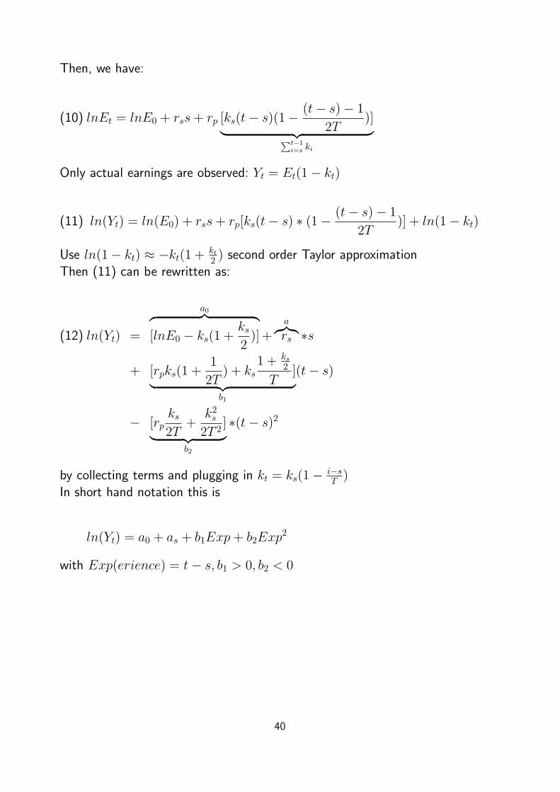
Then, we have:
lnEt = lnE0 + rss+ rp [ks(t− s)(1−(t− s)− 1
2T)]︸ ︷︷ ︸∑t−1
i=s ki
(10)
Only actual earnings are observed: Yt = Et(1− kt)
(11) ln(Yt) = ln(E0) + rss+ rp[ks(t− s) ∗ (1−(t− s)− 1
2T)] + ln(1− kt)
Use ln(1− kt) ≈ −kt(1 + kt2 ) second order Taylor approximation
Then (11) can be rewritten as:
ln(Yt) =
a0︷ ︸︸ ︷[lnE0 − ks(1 +
ks2)]+
a︷︸︸︷rs ∗s(12)
+ [rpks(1 +1
2T) + ks
1 + ks2
T]︸ ︷︷ ︸
b1
(t− s)
− [rpks2T
+k2s2T 2
]︸ ︷︷ ︸b2
∗(t− s)2
by collecting terms and plugging in kt = ks(1− i−sT )
In short hand notation this is
ln(Yt) = a0 + as + b1Exp+ b2Exp2
with Exp(erience) = t− s, b1 > 0, b2 < 0
40

Human Capital Formation
a) Earnings Functions
The causal effect of education on wages
Mincer Earnings Equation: yi earnings
ln(yi) = α + βSi + γ1EXi + γ2EXi2 + εi
Human capital accumulation
Si: Years of schooling(formal education)
β > 0 returns toeducation
EXi: Years of work experi-ence (learning-by-doing,on-the-job training)
γ1 > 0γ2 < 0
returns to ex-perience
• Very successful and often estimated regression
• Increasing wage differences between (and within) skillgroups in various countries (US, UK, . . . )
• Society’s investment in human capital should dependon potential returns
−→ Causal interpretation of β, γ1, γ2 ?
Reference: Card, D. (1999) The Causal Effect ofEducation on Earnings, Handbook of Labor Economics,Vol. 3A.
41

Problems (endogeneity of education and heterogeneity ofreturns to education):
• Ability Bias• Self selection Bias
• Measurement error in education variables
Card’s (1999) human capital model withindividual specific effects
Utility function of individual
(1) U(S, y) = ln(y)− h(S)
S: educational level (years of schooling)y(S): earnings level averaged over work phase
→ being in the labor market: earnings increasewith work experience
h(S): convex cost function describing the disutilityassociated with an additional year of schooling(h′(S) = marginal costs)
Equation (1): condensed version of fully intertem-poral problem
42

Special case: Discounted Present Value (DPV ) Objective
DPV =
∞∫S
y(S) exp(−rt)dt = y(S)exp(−rS)
r
ln(DPV ) = ln(y(S))− (rS + ln(r))︸ ︷︷ ︸h(S)
Optimal Choice of S:
(2)∂U
∂S=y′(S)
y(S)− h′(S) = 0
Special case of DPV :
∂ ln(y)
∂S=y′(S)
y(S)= h′(S) = r Interest rate
Return to education:∂ ln(y)
∂S> r Too little investment in
human capital∂ ln(y)
∂S< r Too much investment
in human capital
All the above assumes log(y(S)) being concave
Individual specific effects:
• Heterogeneity in marginal costs h′(S)
• Heterogeneity in returns ∂ ln(y)∂S = y′(S)
y(S)
43

Simple specification discussed by Card:
y′(S)
y(S)= bi − k1S(3)
h′(S) = ri + k2S(4)
Note:Only the levels bi, ri of the marginal effects differ byindividuals i
Changes of marginal effects k1 > 0, k2 > 0 are constantacross individuals i.
Optimal choice of education:
(5) S∗ =bi − rik1 + k2
=bi − rik
where k = k1 + k2
Comparative Statics: ∂S∗
∂bi> 0 and ∂S∗
∂ri< 0
i.e. individuals with a higher marginal return to S at agiven S choose a higher level of S. With the increase inS, the marginal return to education decreases accordingto equation (3)⇒ Suppose b1 < b2 , then observed difference:
y′(S2)
y(S2)− y′(S1)
y(S1)< b2 − b1
44

• The specification in (3) is used in many empiricalstudies and it is typically assumed that bi is knownwhen making the schooling decision.
Marginal return to education observed:
βi = bi − k1S∗1 = bi
(1− k1
k
)+ ri
k1k
⇒ heterogeneous marginal returns across individualsdepending both on bi and ri !!!
Special cases of constant marginal returns observedβi = constant, if either
a) ri = r and k2 = 0all individuals face the same constant marginalcosts or
b) bi = b and k1 = 0all individuals face the same constant marginalreturns
• Distribution of returns is endogenous in generalequilibrium→ higher supply of highly qualified workers
should reduce the average marginal return
• Assume that return schedules (3) are given from theview point of one cohort of young individuals
45
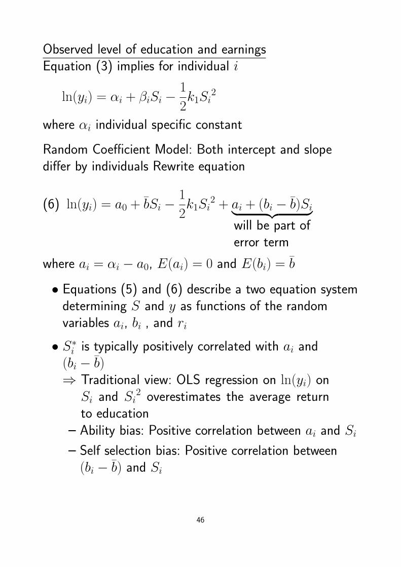
Observed level of education and earningsEquation (3) implies for individual i
ln(yi) = αi + βiSi −1
2k1Si
2
where αi individual specific constant
Random Coefficient Model: Both intercept and slopediffer by individuals Rewrite equation
(6) ln(yi) = a0 + bSi −1
2k1Si
2 + ai + (bi − b)Si︸ ︷︷ ︸will be part oferror term
where ai = αi − a0, E(ai) = 0 and E(bi) = b
• Equations (5) and (6) describe a two equation systemdetermining S and y as functions of the randomvariables ai, bi , and ri
• S∗i is typically positively correlated with ai and(bi − b)⇒ Traditional view: OLS regression on ln(yi) on
Si and Si2 overestimates the average return
to education– Ability bias: Positive correlation between ai and Si
– Self selection bias: Positive correlation between(bi − b) and Si
46
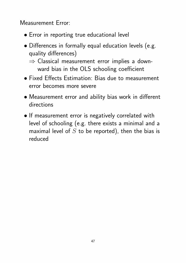
Measurement Error:
• Error in reporting true educational level
• Differences in formally equal education levels (e.g.quality differences)⇒ Classical measurement error implies a down-
ward bias in the OLS schooling coefficient
• Fixed Effects Estimation: Bias due to measurementerror becomes more severe
• Measurement error and ability bias work in differentdirections
• If measurement error is negatively correlated withlevel of schooling (e.g. there exists a minimal and amaximal level of S to be reported), then the bias isreduced
47
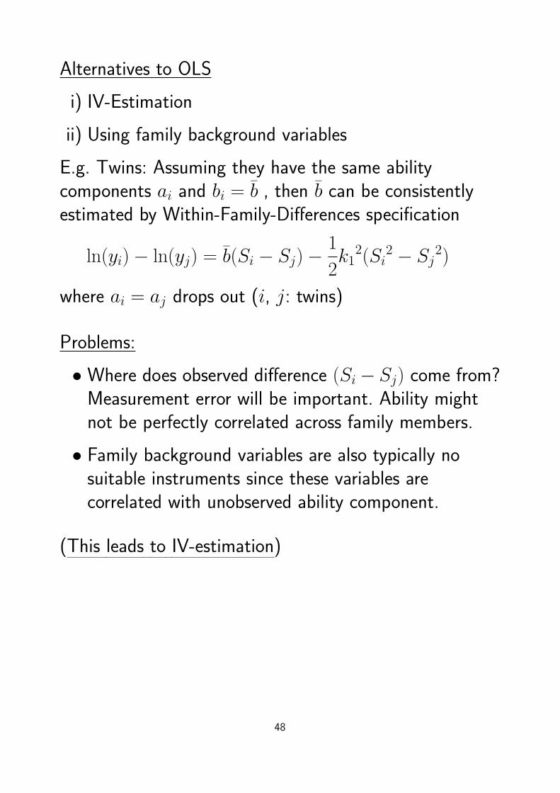
Alternatives to OLS
i) IV-Estimation
ii) Using family background variables
E.g. Twins: Assuming they have the same abilitycomponents ai and bi = b , then b can be consistentlyestimated by Within-Family-Differences specification
ln(yi)− ln(yj) = b(Si − Sj)−1
2k1
2(Si2 − Sj2)
where ai = aj drops out (i, j: twins)
Problems:
• Where does observed difference (Si− Sj) come from?Measurement error will be important. Ability mightnot be perfectly correlated across family members.
• Family background variables are also typically nosuitable instruments since these variables arecorrelated with unobserved ability component.
(This leads to IV-estimation)
48

ad i) IV-Estimation
Supply and Demand considerations suggest to usesupply-side variables Zi as instruments for educationwhere Zi affect the cost of education ri but Zi areuncorrelated with the unobserved ability components aiand bi → Card (2001) Econometrica
Take random coefficients model
(6) ln(yi) = a0 + bSi −1
2k1Si
2 + ai + (bi − b)Si
Assume
ri = Ziπ1 + ηi
where E[ηi|Zi] = E[ai|Zi] = E[(bi − b)|Zi] = 0 i.e. Ziaffect ri and are uncorrelated to ability components aiand (bi − b)
Choice of education:
S∗i =bi − rik
= Z ′iπ + ξi︸︷︷︸=bi−b−ηi
k
49

If Zi is independent of ai, bi − b, and ξi, then b can beestimated consistently with IV but not a0 (with i.i.d. errorterms)
E[Si2|Zi] = E[(Ziπ + ξi)
2|Zi]
= (Ziπ)2 + E[ξi
2|Zi]︸ ︷︷ ︸= constant
E[(bi − b)Si|Zi] = E[(bi − b)Ziπ|Zi]︸ ︷︷ ︸= 0
+E[(bi − b)ξi|Zi]︸ ︷︷ ︸= constant
In general: Independence is a too strong assumption sincea change in Zi affects the entire mapping between abilityand schooling – even though the error terms areuncorrelated with Zi – leading to a systematic correlationbetween (bi − b)Si and Zi !!!
50

• Orthogonality conditions are not sufficient to estimateaverage returns (average slope coefficients) in randomcoefficients model based on standard IV estimation
• Standard IV estimate
(1) Si = Ziπ
(2) ln(yi) = β1 + β2Si + β3Si2
• Estimates: β2, β3 in (2) →
estimate reflects the effect of observedchanges in instruments Zi on educationlevels and the associated changes inearnings for those individuals who areinduced to change their education level inreaction to the observed changes in Zi
LATE: Local Average Treatment Effect
51

Wald–Estimator with Endogenous Dummy Variable
(Important Special Case)
Yi = β0 + δDi + εi mit E{εi|Di} = 0
Coefficient δ (=treatment effect) is constant
and a dummy variable Z = 0, 1 is available as instrument
Wald-IV-Estimator on the basis of two samples {Z = 0} and{Z = 1}
δ =Y Z=1 − Y Z=0
P (D = 1|Z = 1)− P (D = 1|Z = 0)
where P (D = 1|Z = j) =N1,j
Nj
← number {D = 1} in group {Z = j}
← size of group {Z = j}
Wald’s Estimator is equivalent to the 2SLS-estimator for this model
(equation for D is a linear probability model)
⇒ IV-estimator relates induced (=exogenous) change of Y by
instrument variable (Y Z=1−Y Z=0) to the average change of
the endogenous regressor E(D|Z = 1)− E(D|Z = 0).
Local-Average-Treatment-Effect (LATE) Interpretation:
In the presence of heterogeneous effects of the dummy, the
IV-estimator identifies the average effect induced by variation of the
instrument, i.e. the estimated parameter depends on the instrument
(critique by Heckman, 1997, JHR).
52

Extension: Control function approach
(1) Si = Ziπ and ξi = Si − Si(2) E[ln(yi)|Si, Zi]
= a0 + bSi − 12k1Si
2 + λ1ξi + ψ1ξiSi
This is valid if the conditional expectations of ai and biare linear in Si and Zi
E(ai|Si, Zi) = λ1Si + λZZiE((bi − b)|Si, Zi) = ψ1Si + ψZZi
Equation (2) can be estimated consistently based on theresiduals ξi from the first stage regression of Si on theinstruments Ziλ1 = 0 Ability biasψ1 = 0 Self selection bias → consistent estimate for b
53

Generalization of Control Function Approach for Linear Regression
Y1i = Z ′iπ + ε1i
Yi = X ′iγ + αiY1i + εi
= X ′iγ + αY1i + εi + (αi − α)Y1i
Determination of E[εi + ( αi − α︸ ︷︷ ︸ηi
)Y1i|Y1i, Zi]
E{εi|Y1i, Zi} = E{εi|ε1i = Y1i − Z ′iπ} =Cov(εi, ε1i)
V ar(ε1i)· ε1i
E{ηi|Y1i, Zi} =Cov(ε1i, ηi)
V ar(ε1i)· ε1i
Two-stage approach:
1. Regression of Y1i on Zi: ε1i = Y1i − Z ′iπ
2. Regression: Yi = X ′iγ + α Y1i + γ1 ε1i + γ2 Y1i ε1i + εiγ1 = 0: Endogeneity (Durbin-Wu-Hausman Test)
γ2 = 0: Endogenous coefficients (αi are correlated with Y1i)
54
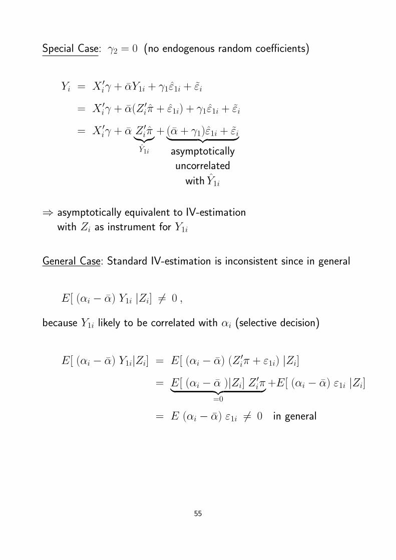
Special Case: γ2 = 0 (no endogenous random coefficients)
Yi = X ′iγ + αY1i + γ1ε1i + εi
= X ′iγ + α(Z ′iπ + ε1i) + γ1ε1i + εi
= X ′iγ + α Z ′iπ︸︷︷︸Y1i
+ (α + γ1)ε1i + εi︸ ︷︷ ︸asymptotically
uncorrelated
with Y1i
⇒ asymptotically equivalent to IV-estimation
with Zi as instrument for Y1i
General Case: Standard IV-estimation is inconsistent since in general
E[ (αi − α) Y1i |Zi] = 0 ,
because Y1i likely to be correlated with αi (selective decision)
E[ (αi − α) Y1i|Zi] = E[ (αi − α) (Z ′iπ + ε1i) |Zi]
= E[ (αi − α )|Zi] Z ′iπ︸ ︷︷ ︸=0
+E[ (αi − α) ε1i |Zi]
= E (αi − α) ε1i = 0 in general
55

Course Material – Section 3. Static Labor Demand
(i) Cost of labor: Wi · Li- Not only wages and salaries, but also auxiliary labor costs,
fluctuation costs, fringe benefits, costs of government regulation.
- Is the wage rate predetermined for a firm? Most likely, this is the
case for contract (union) wages.
→ Additional benefits are not obligatory
Efficiency wage considerations
Monopsony on the labor market
What is Labor demand?
- Persons
- Hours
}effects of reduction of working time (standard hours)
Homogeneous labor is a fiction
(ii) Besides labor, other input factors are used
Here: Capital stock K with the factor price R (capital user costs)
- Substitution, when capital becomes more expensive → LD ↑
- Scale effect, when capital becomes more expensive
→ production and therefore LD falls
(iii) Production technology y = F (L,K)
- Substitution possible between labor and other production factors
- Elasticity of substitution: describes extent by which firm can
substitute labor for capital when wage rises
→ it depends also on technical progress (rationalization and capital
deepening)
56
→ new jobs in other sectors
- Low and high skilled labor
→ complementarity between capital/technical progress and high
skilled labor ?
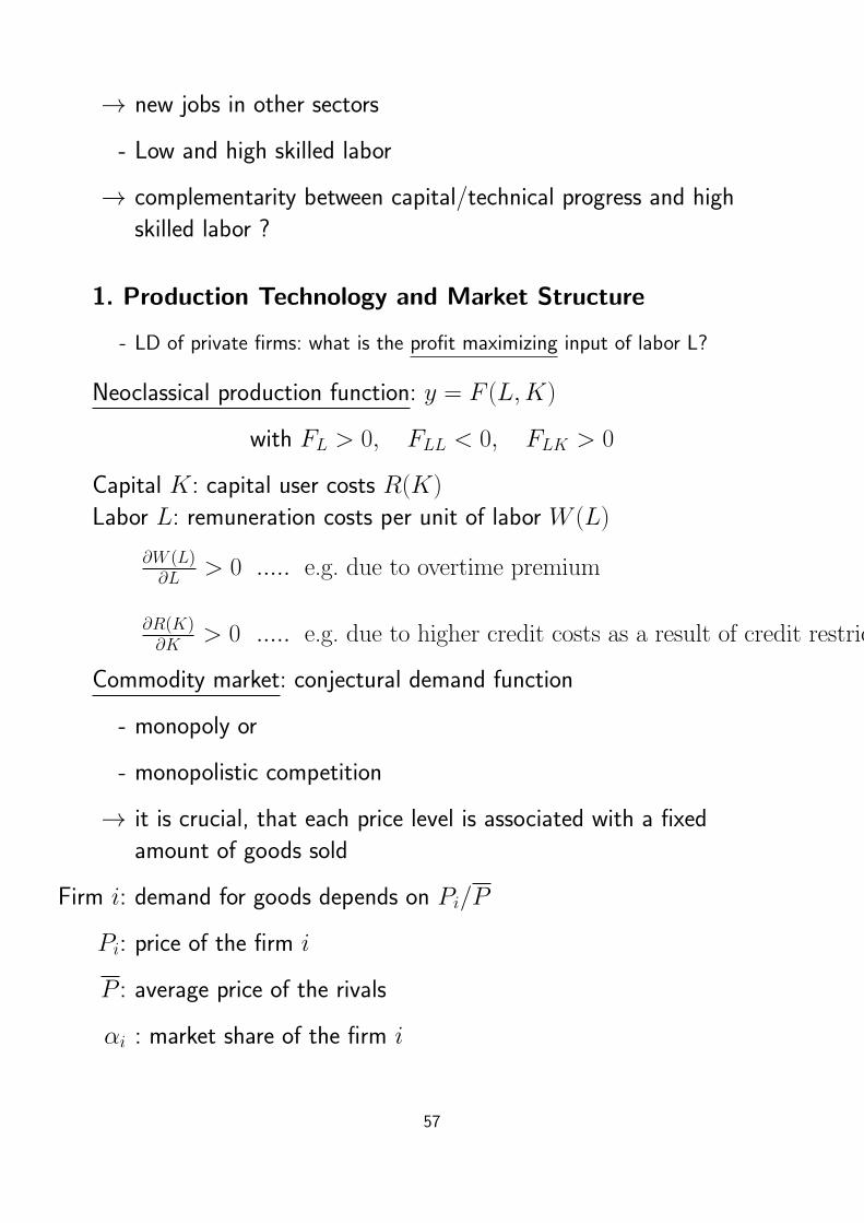
1. Production Technology and Market Structure
- LD of private firms: what is the profit maximizing input of labor L?
Neoclassical production function: y = F (L,K)
with FL > 0, FLL < 0, FLK > 0
Capital K: capital user costs R(K)
Labor L: remuneration costs per unit of labor W (L)
∂W (L)∂L > 0 ..... e.g. due to overtime premium
∂R(K)∂K > 0 ..... e.g. due to higher credit costs as a result of credit restrictions
Commodity market: conjectural demand function
- monopoly or
- monopolistic competition
→ it is crucial, that each price level is associated with a fixed
amount of goods sold
Firm i: demand for goods depends on Pi/P
Pi: price of the firm i
P : average price of the rivals
αi : market share of the firm i
57

αi(Pi/P ) with∂αi
∂(Pi/P )< 0
Aggregate demand:
y(P ) with∂y
∂P< 0
Demand for goods from firm’s i perspective
(4.2) yi = αi(PiP) · y(P ) = yi(Pi, P )
(4.3) ηiyi,P = ∂yi∂Pi· Piyi < 0, ηy,P = ∂y
∂P· Py < 0
- The two elasticities, ηiyi,P = ηy,P , are identical in monopoly case
Note: in what follows, all elasticities are written as absolute
values
- First we analyze variation of Pi at constant P
Profit function for firm i: (without index i except for ηiy,P )
(4.4) Π(L,K, y) = P (y)·y−W (L)·L−R(K)·K−λ·[y−F (L,K)]
• Production function as constraint
First order conditions FOC (differentiate with respect to L, K, y):
(4.5) λ · FL = W · (1 + ηW,L)
(4.6) λ · FK = R · (1 + ηR,K)
(4.7) λ = P ·(1− 1
ηiy,P
)where ηW,L > 0, ηR,K > 0 are relative factor price changes
associated with a change in required quantity of factor input
λ: Lagrange multiplier shows increase in profit when production
increases by one unit
58
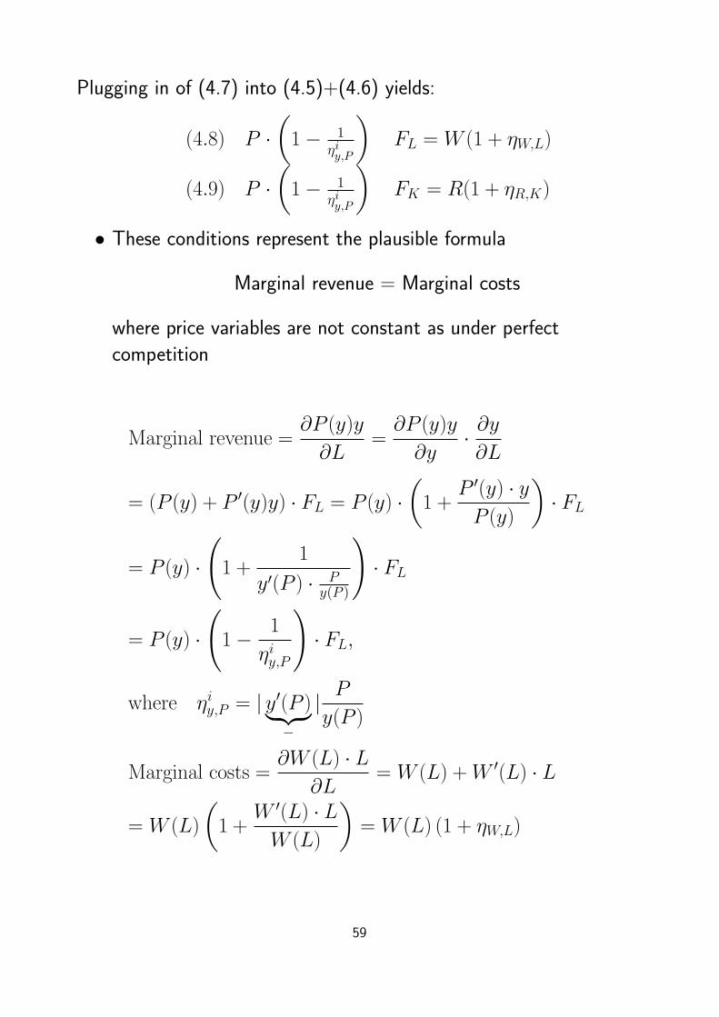
Plugging in of (4.7) into (4.5)+(4.6) yields:
(4.8) P ·(1− 1
ηiy,P
)FL = W (1 + ηW,L)
(4.9) P ·(1− 1
ηiy,P
)FK = R(1 + ηR,K)
• These conditions represent the plausible formula
Marginal revenue = Marginal costs
where price variables are not constant as under perfect
competition
Marginal revenue =∂P (y)y
∂L=∂P (y)y
∂y· ∂y∂L
= (P (y) + P ′(y)y) · FL = P (y) ·(1 +
P ′(y) · yP (y)
)· FL
= P (y) ·
(1 +
1
y′(P ) · Py(P )
)· FL
= P (y) ·
(1− 1
ηiy,P
)· FL,
where ηiy,P = | y′(P )︸ ︷︷ ︸−
| Py(P )
Marginal costs =∂W (L) · L
∂L= W (L) +W ′(L) · L
= W (L)
(1 +
W ′(L) · LW (L)
)= W (L) (1 + ηW,L)
59
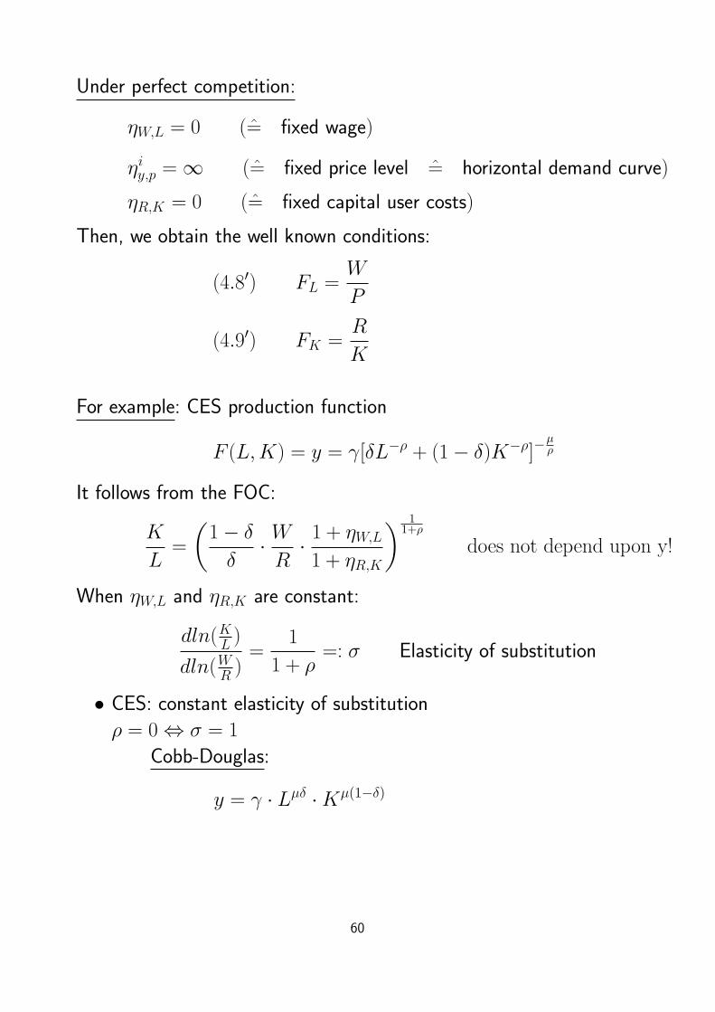
Under perfect competition:
ηW,L = 0 (= fixed wage)
ηiy,p =∞ (= fixed price level = horizontal demand curve)
ηR,K = 0 (= fixed capital user costs)
Then, we obtain the well known conditions:
(4.8′) FL =W
P
(4.9′) FK =R
K
For example: CES production function
F (L,K) = y = γ[δL−ρ + (1− δ)K−ρ]−µρ
It follows from the FOC:
K
L=
(1− δδ· WR· 1 + ηW,L1 + ηR,K
) 11+ρ
does not depend upon y!
When ηW,L and ηR,K are constant:
dln(KL )
dln(WR )=
1
1 + ρ=: σ Elasticity of substitution
• CES: constant elasticity of substitutionρ = 0⇔ σ = 1
Cobb-Douglas:
y = γ · Lµδ ·Kµ(1−δ)
60
2. Factor price changes and labor demand- For simplification:
• Perfect competition in the input market (W and R exogenous)
• Linear homogeneous production function
Reaction of LD in response to factor price changes
(i) substitution effect: firm uses less of the factor, which became
comparatively more expensive
→ movement on an isoquant
e.g.: if W increases or R declines, the firm uses less labor
(ii) scale effect:
a) Rise in the factor price reduces the profit maximizing output
and therefore the amount of input factors needed
→ rise in wages clearly causes a lower use of labor
→ rise in capital costs has this effect only in case, when
scale effect overcompensates substitution effect
b) the purchasing power effect arising from a wage increase
shifts goods demand function to the right after substraction
of scale effect losses
→ practically irrelevant in the micro-economic partial
analysis
Here, we abstract from the purchasing power effect of
wage increase
We are interested in factor demand elasticities:
ηL,W =∂L
∂W· WL
and ηL,R =∂L
∂R· RL
61
Derivation (unfortunately quite involved): Firm i
- In initial situation: production = sales (no storage)
– Marginal Value Product (corrected for goods demand
elasticities) matches factor price
(1) y(P, P ) = F (L,K)
(2) W = FL · P ·(1− 1
ηiy,p
)(3) R = FK · P ·
(1− 1
ηiy,p
)- if all firms react to factor price changes by adjusting their prices,
the assumption of P being constant has to be given up
→ for symmetric firms: dP = dP
As a simplification, we can write then:
(4) y(λ) = F (L,K) with λ = P
(1− 1
ηiy,p
)(5) W = FL · λ(6) R = FK · λ
To determine the effect of a change in wages, equations (4)-(6) have
to be differentiated with respect to W :
(7) − ∂λ
∂W· ηy,λ ·
y
λ= FL
∂L
∂W+ FK ·
∂K
∂W
(8) 1 = FL ·∂λ
∂W+ λ ·
(FLL ·
∂L
∂W+ FLK ·
∂K
∂W
)62
(9) 0 = FK ·∂λ
∂W+ λ ·
(FKL ·
∂L
∂W+ FKK ·
∂K
∂W
)Because of results for linearly homogeneous production functions, we
obtain
(7′) y · ηy,λ ·∂λ
∂W+W · ∂L
∂W+R
∂K
∂W= 0
(8′) y · σ ∂λ∂W− K
L·R · ∂L
∂W+R
∂K
∂W=y · λW
σ
(9′) y · σ ∂λ∂W
+W∂L
∂W− L
K·W · ∂K
∂W= 0
To determine ∂L∂W , apply Cramer’s rule:
- Because it is very involved, I now present only the results (please
check on your own!)
(10)∂L
∂W= − L
W
(L ·Wy · λ
· ηy,λ +R ·Ky · λ
σ
)so that
(11) ηL,W ≡∂L
∂W· WL
= −
L · FLy︸ ︷︷ ︸SL
ηy,λ +K · FKy︸ ︷︷ ︸
SK=1−SL
·σ
Production elasticities correspond to shares:
∂lnY
∂lnK= sK and
∂lnY
∂lnL= sL
This results in:
(12) ηL,W = −sLηy,λ − (1− sL)σ
Under perfect competition:
(13) ηL,W = −sLηy,p − (1− sL)σ
63

since ηy,λ = ηy,p due to ηiy,p =∞
Again:
ηL,W = −sL ηy,p︸ ︷︷ ︸scale effect︸ ︷︷ ︸big if sL big
− (1− sL)σ︸ ︷︷ ︸substitution effect︸ ︷︷ ︸small if sL big
Note: Both terms are unambiguously negative
ηy,p: Sensitivity of aggregate demand with respect to the increase in
prices in all firms
- Difference between (12) and (13):
λ =MR = P(1− 1
ηiy,p
)is in (12) the basis for the firm’s decision making
↑ (monopolistic competition)
Marginal revenue
→ labor demand effect in (12) is weaker because MR increases at
lower y
In an analogous manner to ηLW , one can derive ηL,R (cross price
elasticity) for perfect competition:
(14) ηL,R = (1− sL) · ( σ − ηy,p)
+ -
subst. scale effect
effect
- Reduction in capital user costs results in higher employment only
if the scale effect dominates
64

It follows from (13) and (14):
(15) ηLW+ηLR = −=0︷ ︸︸ ︷
(1− sL)σ + (1− sL)σ−sLηy,p+(1−sL)ηy,p= −ηy,p < 0
- When W and R increase by the same relative amount (in percent),
then only scale effect operates → employment falls
3. Profit maximization versus cost minimization
• Because of methodical considerations and in light of available
data for empirical work: alternative illustration of production
technology using duality theory based on cost function
6
-
r
@@@
@@@@
@@@
@@
K
−wR L
y
- Cost-minimizing use of factors
C = R ·K +W · L = C
K =C
R− W
RL
minC = WL +RK
s.t. : y = F (L,K)
}L = WL +RK + λ[y − F (L,K)]
FOC:∂L∂L = W − λFL = 0∂L∂K = R− λFK = 0
}W
R=FLFK
65

∂L∂λ
= y − F (L,K) = 0
- The first two FOC correspond to those under profit maximization
in case of perfect competition on the factor markets
- The factor demand in case of cost minimization arises as a
function of factor prices (W,R) and output y
L = L(W,R, y)
K = K(W,R, y)
}zero homogeneous in factor prices
C = C(L(W,R, y), K(W,R, y)) = C(W,R, y)
According to Shephard’s Lemma:
L =∂C(W,R, y)
∂WK =
∂C(W,R, y)
∂R
⇒ The cost function incorporates the same information about the
technology as the production function (cost function and production
function are dual to each other)
⇒ These relationships are very important for the empirical analysis.
Example:
C = y ·W α ·R1−α
Applying Shepard’s Lemma:
L =∂C
∂W= y · α ·W α−1 ·R1−α = y · α ·
(R
w
)q−αK =
∂C
∂R= y · (1− α) ·W α ·R−α = y · (1− α)
(W
R
)α
66
Solving both equations for
(W
R
):
(W
R
)1−α=yα
L⇔ W
R=
(yα
L
) 11−α
W
R=
(y(1− α)
K
)− 1α
(yαL
) 11−α
=
(y(1− α)
K
)− 1α
⇔ y1
1−α +1α = α
− 11−αL
11−α · (1− α)−
1αK
1α
⇔ yα+1−αα(1−α) = α
− 11−α(1− α)−
1αL
11−αK
1α
⇔ y = α−α(1− α)−(1−α)︸ ︷︷ ︸A
LαK1−α
i.e. Cobb-Douglas cost function is dual to Cobb-Douglas production
function.
General 2nd order approximation of cost function (Translog cost
function):
ln(C) = c0 + a1ln(y) + 0.5a2ln(y)2 + a3ln(y)ln(W )
+a4ln(y)ln(R) + c1ln(W ) + 0.5c2ln(W )2
+c3ln(W )ln(R) + 0.5c4ln(R)2
+c5ln(R) + β1t + β2ln(W )t + β3ln(R)t
67
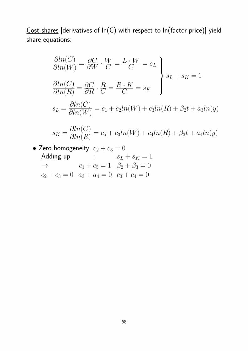
Cost shares [derivatives of ln(C) with respect to ln(factor price)] yield
share equations:
∂ln(C)∂ln(W )
= ∂C∂W· WC = L ·W
C = sL
∂ln(C)∂ln(R)
= ∂C∂R· RC = R ·K
C = sK
sL + sK = 1
sL =∂ln(C)∂ln(W )
= c1 + c2ln(W ) + c3ln(R) + β2t + a3ln(y)
sK =∂ln(C)∂ln(R)
= c5 + c3ln(W ) + c4ln(R) + β3t + a4ln(y)
• Zero homogeneity: c2 + c3 = 0Adding up : sL + sK = 1
→ c1 + c5 = 1 β2 + β3 = 0
c2 + c3 = 0 a3 + a4 = 0 c3 + c4 = 0
68
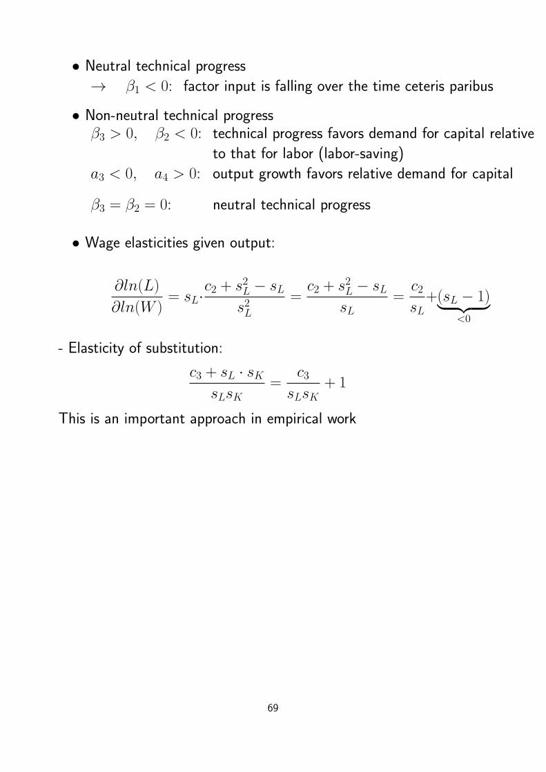
• Neutral technical progress→ β1 < 0: factor input is falling over the time ceteris paribus
• Non-neutral technical progressβ3 > 0, β2 < 0: technical progress favors demand for capital relative
to that for labor (labor-saving)
a3 < 0, a4 > 0: output growth favors relative demand for capital
β3 = β2 = 0: neutral technical progress
• Wage elasticities given output:
∂ln(L)
∂ln(W )= sL·
c2 + s2L − sLs2L
=c2 + s2L − sL
sL=c2sL
+(sL − 1)︸ ︷︷ ︸<0
- Elasticity of substitution:
c3 + sL · sKsLsK
=c3
sLsK+ 1
This is an important approach in empirical work
69
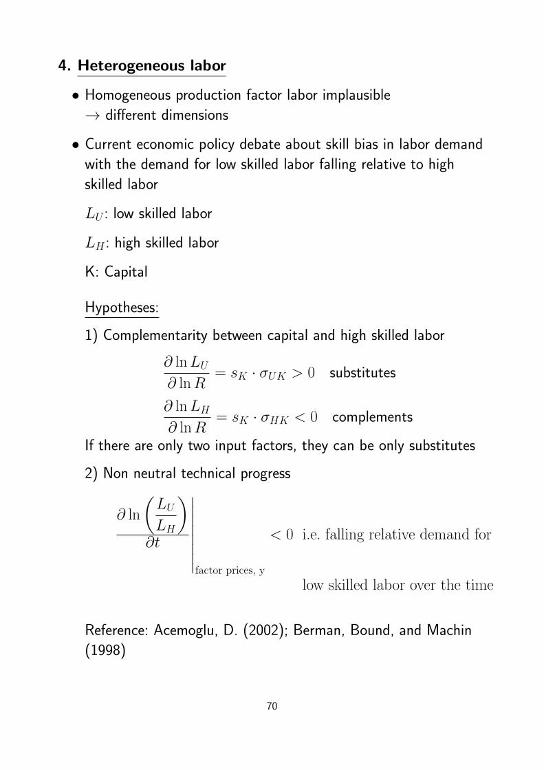
4. Heterogeneous labor
• Homogeneous production factor labor implausible
→ different dimensions
• Current economic policy debate about skill bias in labor demand
with the demand for low skilled labor falling relative to high
skilled labor
LU : low skilled labor
LH : high skilled labor
K: Capital
Hypotheses:
1) Complementarity between capital and high skilled labor
∂ lnLU∂ lnR
= sK · σUK > 0 substitutes
∂ lnLH∂ lnR
= sK · σHK < 0 complements
If there are only two input factors, they can be only substitutes
2) Non neutral technical progress
∂ ln
(LULH
)∂t
∣∣∣∣∣∣∣∣factor prices, y
< 0 i.e. falling relative demand for
low skilled labor over the time
Reference: Acemoglu, D. (2002); Berman, Bound, and Machin
(1998)
70

Heterogeneous demand for labor, skill biased technologicalchange (SBTC), globalization, and institutionsReference: Acemoglu, D. (2002) Technical Change, Inequality, and
the Labor Market. Journal of Economic Literature.
Stylized view: The increase in earnings inequality in the UK/US and
the rise in unemployment rates in continental Europe during the 80s
and 90s reflect an increase in the relative demand for more highly
skilled labor since the relative supply of more highly skilled labor has
increased at the same time.
Framework mostly used to study these developments: Supply,
demand, and institutions SDI
Two skill groups: S skilled
U unskilled
NS, NU employment
wS, wU wages
71

ln(wSwU
)
ln(NSNU
)
w1
w0
N0 N1
S0 S1
D0
D1A
C
D
B
Change from period 0 to period 1:
• Inelastic relative supply increases from N0 to N1
• Labor demand increases from D0 to D1
We observe
• higher skill differential in wages w1 in period 1 compared to w0
in period 0 and
• higher relative employment of skilled workers N1 in period 1
relative to N0 in period 0
72

→ The increase in demand at a given wage ratio was larger than
the increase in supply
⇒ Search for reasons why relative demand has changed: SBTC,
change in product demand across industries with different skill
intensities e.g. through increasing international trade
Institutional effects:
Intersection of supply and demand curves describes competitive
equilibrium
→ Rents for groups of workers can change over time
→ Minimum wages (e.g. through unions) can prevent wage adjust-
ment in equilibrium: If wage remains at old level w0, the relative
demand NSNU
exceeds the relative supply resulting in unemploy-
ment of the unskilled workers
73

Formalization based on a CES-Produktion Function
Output: Constant returns to scale
Qt = [αt(atNst)ρ + (1− αt)(btNut)
ρ]1ρ
Nst, Nut: skilled/unskilled employment in period t
σ = 11−ρ: elasticity of substitution and ρ ≤ 1 ⇔ σ > 0
αt: share of activity assigned to skilled employ-
ment
at, bt: skilled/unskilled labor augmenting technical
progress
Skill biased technical change (SBTC)
Increases in atbtor αt
atbt↑ intensive SBTC: skilled workers become relatively
better at existing jobs
αt ↑ extensive SBTC: ”upskilling” of work tasks
74

If both input factors are paid by their marginal products
wstwut
=αt
1− αt·(atbt
)ρ·(Nst
Nut
)− 1σ
In logarithms:
ln
(wstwut
)= ln
(αt
1− αt
)+ ρ ln
(atbt
)︸ ︷︷ ︸
technical progress
− 1
σln
(Nst
Nut
)︸ ︷︷ ︸
supply
This equation explains the skill differential in wages as the result of
relative factor supplies (× inverse of elasticity of substitution) and
technical progress shifting relative labor demand.
Only for ρ > 0 (i.e. σ > 1) does a skill bias in entensive technical
progress (atbt ↑) yield a higher skill differential in wages.
75