Topics in generating functions

Qiaochu YuanMassachusetts Institute of Technology

Department of Mathematics

Written for the Worldwide Online Olympiad Training programhttp://www.artofproblemsolving.com

April 7th, 2009

1 Introduction

Suppose we want to study a sequence a0, a1, a2, .... Such a sequence might be defined bya recurrence relation we’re given, or it might count some family of sets. There are manyspecific classes of sequences with very different properties, so what general methods exist tostudy sequences? The general technique we’ll discuss here is that of studying a sequence bystudying its Z-transform, or generating function

A(x) = a0 + a1x+ a2x2 + ... =

∑n≥0

anxn. (1)

An obvious advantage of this representation is that it’s a very compact way of describingmany simple sequences: for example, geometric series can be written as

a+ arx+ ar2x2 + ... =a

1− rx

which is just the statement of the geometric-series-summation formula. You can thinkof the introduction of the parameter x as useful because it allows you to restrict to x smallenough so that we have convergence regardless of the value of r, but you don’t really needcalculus to understand generating functions: for most purposes it’s more convenient to regardgenerating functions as formal and ignore questions of convergence. The ring of formal powerseries, denoted C[[x]], consists of infinite sums of precisely the above form, with additiondefined by

(a0 + a1x+ ...) + (b0 + b1x+ ...) = (a0 + b0) + (a1 + b1)x+ ... (2)

and multiplication defined by

(a0 + a1x+ ...)(b0 + b1x+ ...) = c0 + c1x+ ..., cn =n∑k=0

akbn−k. (3)

(cn) is called the convolution of the sequences (an) and (bn). One big advantage of thegenerating function approach is that convolution is a natural operation on many sequencesof combinatorial interest and that talking about multiplying functions is easier than writingdown convolutions. But as we’ll see, the value of the generating functions approach is muchdeeper than this.

Example Denote the probability of rolling a sum of n with d six-sided dice by pn,d. Clearlyone rolls a sum of n by rolling a sum of n− k with the first d− 1 dice and rolling a sum ofk on the last die; in other words, we have the recurrence

pn,d =pn−1,d−1 + pn−2,d−1 + ...+ pn−6,d−1

6.

This recurrence is difficult to work with until we realize that it is a convolution andequivalent to the following identity:

1

∑n≥0

pn,dxn =

(x+ x2 + ...+ x6

6

)(∑n≥0

pn,d−1xn

)

=

(x+ x2 + ...+ x6

6

)d.

Note that, as expected, this identity tells us that the probability of rolling a sum lessthan d is zero and that the probability of rolling a sum of either d or 6d is 1

6d. The generating

function x+x2+...+x6

6is just p1,1x + p2,1x

2 + ..., the function that describes the probability ofrolling each face on a six-sided die.

Now here’s a computation you really don’t want to do without generating functions: thefactorization

x+ x2 + ...+ x6 = x

((x3 − 1)(x3 + 1)

x− 1

)= x(x+ 1)(x2 + x+ 1)(x2 − x+ 1),

which implies the following factorization:

(x+ x2 + ...+ x6)2 = x(x2 + 1)(x2 + x+ 1) · x(x2 + 1)(x2 + x+ 1)(x2 − x+ 1)2

= (x+ 2x2 + 2x3 + x4)(x+ x3 + x4 + x5 + x6 + x8).

What this means, interpreted combinatorially, is as follows: the probability distributionof rolling two normal six-sided dice is the same as the probability distribution of rolling adie with sides 1, 2, 2, 3, 3, 4 and sides 1, 3, 4, 5, 6, 8, and in fact substituting x = 1 and playingaround with the factors above should convince you that this is the only other pair of six-sideddice for which this is true. A fact like this, which might seem to require a lot of tediouscasework to verify, follows directly from the factorization of polynomials of the form xn − 1into their irreducible factors, known as cyclotomic polynomials.

In harder combinatorial problems, the sequence of interest won’t have a nice formulaeven though it has a nice generating function. For example, the number of partitions p(n) ofa positive integer n into a sum of other positive integers (ignoring order) has the beautifulgenerating function ∑

n≥0

p(n)xn =1

(1− x)(1− x2)(1− x3)....

While sequences like p(n) don’t have ”nice” closed forms, we can learn two very interestingthings from this generating function: multiplying out the denominator (which is harderthan it sounds), Euler obtained his pentagonal number theorem, which implies the beautifulrecursion

p(k) = p(k − 1) + p(k − 2)− p(k − 5)− p(k − 7) + p(k − 12) + p(k − 15)−−+ +....

2

While it is possible to give a combinatorial proof of this result, it’s hard to imagine thatit could’ve been discovered without generating functions. And the power of the generatingfunction doesn’t step there: analytic arguments allow us to deduce the asymptotic

p(n) ∼ 1

4√

3neπ√

2n3 .

This beautiful result, due to Hardy and Ramanujan, is uniquely analytic. While we won’tdiscuss the methods by which such estimates are obtained, it’s good to keep in mind thatgenerating functions can give us genuinely new information; see [6].

For combinatorialists, generating functions make the proof of certain combinatorial iden-tities so easy in some cases that there are various combinatorial identities whose only proofsare via generating functions and for which a combinatorial proof isn’t known. Hence gen-erating functions also provide us with a rich source of difficult and interesting identities toexplain.

1.1 What a ”problem-solver” needs to know

There’s a good reason to learn how to use generating functions properly, even if they don’tshow up too often on Olympiads: if you figure out what generating function to use on aproblem, it tends to become very easy (at least, compared to other Olympiad problems). Soit’s a good idea to learn how to solve them in case they do show up!

This is not to say that it is always possible to apply these techniques automatically. Oftenfiguring out the generating function becomes the main challenge of the problem. Fortunately,there are fairly systematic ways to do this, which we will attempt to cover. Keep the followinggeneral strategies and principles in mind as you read the specific strategies in the rest of thispaper.

1. Be familiar with the simplest generating functions so you can recognize their coefficientswhen they appear in problems. (You’ll know what these are once you’re done reading.)

2. See if the problem statement implies a recursion. Recursions imply generating functionidentities.

3. Many natural operations on generating functions (multiplying by x, differentiating)are linear operators. If a computation seems difficult to do for a specific function Fbut it is easy to do for a class of functions F and it is linear, see if you can write F asa sum of functions in F . (This might be called the Fourier-analytic point of view.)

4. If a summation seems symmetric, it might be the result of a product of generatingfunctions. The simplest example is the sum

∑akbn−k, which can be written more

symmetrically as∑

i+j=n aibj. The sum∑

i+j+k=n aibjck, for example, is a product ofthree generating functions.

3

5. If you know the closed form of a single generating function F , you know the closed formof any generating function you can get by manipulating F and you can compute anysum you can get by substituting specific values into any of those generating functions.

6. Special cases are harder than general cases because structure gets hidden. If youintroduce extra variables, you might figure out what the general case is and you cansolve that instead. On the other hand, there is more than one way to introduce avariable into a problem.

7. Exchanging orders of summation can turn difficult computations into simple ones. [6]has some very good examples.

8. Sequences don’t have to be numbers.

4

2 Basic results

Given a sequence (an), we call the associated function A(x) =∑

n≥0 anxn its ordinary

generating function, or ogf for short. There are many other kinds of generating function,but we’ll explore this case first. Given a function A(x), the notation [xn]A(x) denotes thecoefficient an of xn. Adding generating functions is easy enough, but multiplication is worthdiscussing.

Definition Given two generating functions A(x) =∑

n≥0 anxn, B(x) =

∑n≥0 bnx

n, theirproduct AB is the generating function C(x) =

∑n≥0 cnx

n with coefficients

cn =n∑k=0

akbn−k. (4)

(cn) is called the Cauchy product or convolution of (ak) and (bk).

The following suggests a combinatorial motivation for this definition.

Proposition 2.1. If A is a family of sets and ak is the number of sets of ”weight” k in Aand B is a family of sets such that bk is the number of sets of ”weight” k in B, then cn isthe number of pairs of a set from A and a set from B of total ”weight” n. We can thereforewrite

A(x) =∑a∈A

x|a|, B(x) =∑b∈B

x|b|, C(x) =∑

c=(a,b)∈A×B

x|c| (5)

where |a| is the weight of a and |c| = |a| + |b| (by definition). We call A(x) the weightenumerator of A.

Note that the definition of weight is arbitrary: that’s what makes this idea so powerful.Algebraically, this is the definition we would expect if we simply required that formal seriesmultiply like polynomials, but as the combinatorial interpretation of the definition shows, itis both very general and usually the ”correct” multiplication to think about combinatorially.If you think of the sets A,B as being ”combinatorial sets,” then C can be thought of astheir ”combinatorial Cartesian product”; this is the point of view taken up by species theory,which we will not discuss further, but the interested reader can consult [1].

Example Let A be the family of subsets of an n-element set X with weight the number ofelements in a subset, and let B be the family of subsets of an m-element set Y , likewise. Anordered pair of a subset of X and a subset of Y determines a subset of the disjoint unionX t Y , which has m+ n elements. Thus(

m+ n

k

)=

k∑i=0

(m

i

)(n

k − i

).

In generating function terms, (1 + x)m+n = (1 + x)m(1 + x)n. This is known as Vander-monde’s identity, and we will return to it later.

5

Note that convolution is very different from the pointwise or Hadamard product∑

n≥0 anbnxn,

which is in general very difficult to compute given only A,B.While multiplication is natural to look at combinatorially, there are more natural oper-

ations on a single sequence.

Proposition 2.2. Let A(x) =∑

n≥0 anxn be the generating function of (an) and define

sn = a0 + ...+ an. Then

S(x) =∑n≥0

snxn =

A(x)

1− x= A(x) (1 + x+ ...) . (6)

Corollary 2.3. Define d0 = a0, dn = an − an−1. Then

D(x) =∑n≥0

dnxn = (1− x)A(x). (7)

We call the transformation (an) 7→ (dn) the (backward) finite difference operator and willwrite dn = ∇an. Later we will discuss both of these transformations in more depth, but firstan application.

Example The harmonic numbers Hn are defined by Hn = 1 + 12

+ ... + 1n. Compute their

generating function.

Proof. We simply need to take the partial sums of the generating function∑

n≥1xn

n. With

some familiarity with calculus, you might recognize this as the generating function of ln 11−x ;

it then follows that ∑n≥1

Hnxn =

1

1− xln

1

1− x.

Let P (x) =∑

n≥0 pnxn describe the probabilities of rolling various faces of a die (which

can be finite or infinite; that is, P can be either a polynomial or a formal series); pn is theprobability of rolling face n, and we require that pn ≥ 0∀n and P (1) = 1. We can thereforededuce the following from definition, which is very convenient.

Proposition 2.4. The expected value of a dice roll with generating function P is P ′(1).

Generally, given a generating function for a sequence (an) we can easily compute thegenerating function for the sequence (nan).

Proposition 2.5. Given A(x) =∑

n≥0 anxn, the generating function for nan is x d

dxA(x).

Thus to multiply a sequence by a polynomial (equivalently, to take a Hadamard productof a sequence with a polynomial) all we have to do is repeatedly differentiate and multiply byx. We often abbreviate the derivative as D, and so the above can be understood as applying

6

an operator xD repeatedly. To multiply by higher-degree polynomials, apply xD repeatedly(that is, take it to various powers) and add the results.

Applying xD repeatedly to the generating function 11−x tells us how to compute the

generating function of any polynomial.

Corollary 2.6. The generating function of a polynomial p(x) is p(xD)(

11−x

).

If p(x) =∑n

i=0 pixi, then p(xD) is shorthand for the operator

∑ni=0 pi(xD)i, which means

”for each i, apply the differential operator xD i different times, multiply by pi, and add theresults obtained.” This is an annoying computation to perform for polynomials of evenmoderate degree. In the next section we present an alternate method for computing thegenerating function of polynomials.

Example You have a coin that flips heads with probability p and tails with probability1 − p. Flip the coin until you flip tails. What is the expected value of the square of thenumber of flips necessary for this to occur?

Proof. The probability of flipping heads n times and flipping tails is pn(1− p), which gives

P (x) =∑k≥0

pk(1− p)xk =1− p

1− px.

Note that P (1) = 1 as is necessary. (This is a probabilistic proof of the geometric seriessummation formula.) We now have to compute

∑k2pk(1 − p). We readily compute that

xD(

11−px

)= px

(1−px)2 and

xD

(px

(1− px)2

)=

px

(1− px)2+

2p2x2

(1− px)3

hence we find that ∑k≥0

k2pk(1− p)xk =(1− p)(px+ p2x2)

(1− px)3.

Substituting x = 1 gives p(1+p)(1−p)2 .

A remark is in order. The derivative on formal power series is purely a formal operation.It does not require any notion of a limit; it is defined by what it does to each term, and assuch it is valid for coefficients in any ring. This observation will be of use later. In any case,if the derivative can be defined formally, then so can the integral, which has the followingconsequence.

Proposition 2.7. Given A(x) =∑

n≥0 anxn, the generating function for an

n+1is∫ x

0A(t) dt.

This observation is the basis for concocting rather difficult-looking identities.

7

Example Compute∑n

k=01

k+1

(nk

). (This is one of the less difficult-looking ones.)

Proof. We merely have to integrate the generating function for the binomial coefficients,which gives ∫ 1

0

(1 + t)n dt =(1 + t)n+1 − 1

n+ 1,

and substituting t = 1 we obtain the answer 2n+1−1n+1

.

8

2.1 Exercises

Generally the exercises will vary wildly in difficulty and not really be arranged in order ofincreasing difficulty.

1. What is the expected size of a random subset of {1, 2, ...n}?

2. USAMO 1989 #1: For each positive integer n, let

Sn = 1 +1

2+ ...+

1

n

Tn = S1 + S2 + ...+ Sn

Un =T1

2+T2

3+ ...+

Tnn+ 1

.

Find, with proof, integers 0 < a, b, c, d < 10000 such that T1988 = aS1989 − b andU1988 = cS1989 − d.

3. For a, b positive integers, compute

b∑i=0

(−1)b−i1

a+ b− i

(b

i

).

4. (a) (Almost) USAMO 1996 #6: Determine (with proof) whether there is a subsetX of the non-negative integers with the following property: for any non-negativeinteger n there is exactly one solution of a+ 2b = n with a, b ∈ X.

(b) Putnam 2003 A6: For a set S of non-negative integers let rS(n) denote the numberof ordered pairs of distinct elements s1, s2 ∈ S such that s1 + s2 = n. Is itpossible to partition the non-negative integers into disjoint sets A and B suchthat rA(n) = rB(n) for all n?

5. USAMO 1991 #2: For any nonempty set S of numbers, let σ(S) and π(S) denote thesum and product, respectively, of the elements of S. Prove that∑ σ(S)

π(S)= (n2 + 2n)−

(1 +

1

2+ ...+

1

n

)(n+ 1)

where∑

denotes a sum involving all nonempty subsets of {1, 2, ...n}.

9

3 Polynomials, finite differences, and summations

If functions of the form 1(1−x)n have coefficients which are polynomials, perhaps it would

be worthwhile to figure out 1) exactly what polynomials these are, and 2) how to write anarbitrary polynomial as a linear combination of such polynomials. This would, in principle,be easier than repeated differentiation. If we could do so, it would be very easy to figure outthe answer to evaluate sums such as

n∑k=0

k3

since all we would have to do is compute∑

k≥0 k3xk and multiply it by 1

1−x as we haveseen. A generalization of Proposition 2.3 turns out to be exactly what we need. Recall that∇an = an − an−1.

Proposition 3.1. Let ∇0an = an,∇k+1an = ∇(∇kan). If A(x) =∑

n≥0 anxn, then∑

n≥0

∇kanxn = (1− x)kA(x). (8)

Corollary 3.2. Let San = a0 + a1 + ...+ an, and S0an = an,Sk+1an = S(Skan). Then∑

n≥0

Skanxn =

A(x)

(1− x)k(9)

The proposition explains why taking repeated finite differences of a generic sequence getsyou binomial coefficients, if you have ever observed this pattern without understanding it.But if we understand the coefficients of (1− x)n, what are the coefficients of 1

(1−x)n ? Whenn = 0, this is the generating function of the sequence 1, 0, 0, 0, .... Repeatedly taking partialsums gives us the following family of sequences:

1 1 1 1 1 . . .1 2 3 4 5 . . .1 3 6 10 15 . . .1 4 10 20 35 . . .1 5 15 35 70 . . ....

......

......

. . .

The obvious conjecture immediately presents itself: this is Pascal’s triangle turned side-ways! This matrix is referred to as the (infinite) symmetric Pascal matrix. The constructionwe presented above is equivalent to the usual construction of Pascal’s triangle, and it impliesthe following result.

Proposition 3.3. The coefficient of xk in 1(1−x)n is

(n+k−1n−1

), a polynomial of degree n− 1.

10

Corollary 3.4. ∑n≥0

(n

k

)xn =

xk

(1− x)k+1.

Pascal’s triangle, however, is not the end of the story. The product of (1+x+x2+...) withitself n times counts the number of solutions, in non-negative integers, to a1+a2+...+an = k.This is because we can think of evaluating this product as choosing xa1 from the first factor,xa2 from the second factor, and so forth. We can then understand the above result as follows:there are n distinguishable urns into which we want to place k indistinguishable balls; thenumerical value of ai is the number of balls in urn i. To solve the problem combinatorially,consider a string of symbols, one for each of the k balls and n − 1 other divider symbols.There are clearly

(n+k−1n−1

)ways of arranging these symbols. On the other hand, given any

arrangement of balls and dividers we can take the set of balls before the first divider tobelong in the first urn, the balls between the first and second divider to belong in the secondurn, and so forth.(

n+k−1k

)is also the number of multisets of k elements among n elements of a set. A

multiset is a set into which an element may be placed more than once; the number ofmultisets of k elements from n elements is denoted

((nk

)). Now, an application.

Example Compute the probability of rolling a sum of 18 on 4 six-sided dice.

Proof. This is the coefficient of x18 in(x+x2+...+x6

6

)4

, but how do we actually compute it

without going through a lot of tedious expansion? First, we can recognize that by thesymmetry of the coefficients the coefficient of x18 is equal to the coefficient of x10: in balls-and-urns terms, instead of solving the equation a + b + c + d = 18 where 1 ≤ a, b, c, d ≤ 6we can equivalently solve (7− a) + (7− b) + (7− c) + (7− d) = 10. Now for the importantstep: factor as

x4

64

(1− x6

1− x

)4

.

Now we only have to compute the coefficient of x6 in (1− x6)4 · 1(1−x)4 , and we know the

coefficients in both of those now! The x6 term of the right factor is(6+4−1

3

)=(93

)and there

is an additional term −4x6 from the left factor, so our final answer is(93

)− 4

64.

The combinatorial interpretation of the above argument is essentially inclusion-exclusion:first we count all solutions to a+b+c+d = 16 (or 12) by balls-and-urns, then we subtract thesolutions where one of a, b, c, d is greater than 6, and so forth. Of course, this generalizes.

Thinking of 1(1−x)n as (1 − x)−n suggests the following generalization of the binomial

theorem, which was proven by Newton.

11

Theorem 3.5. For α ∈ C and a non-negative integer k, define(α

k

)=α(α− 1)...(α− (k − 1))

k!. (10)

Then

(1 + x)α =∑n≥0

(α

n

)xn. (11)

The polynomial(αk

)is sometimes called a Newton polynomial of degree k. It specifies to

the usual binomial coefficient when α is a non-negative integer.

Proof. The kth derivative of (1 + x)α is k!(αk

)(1 + x)α−k by induction, so this follows by the

familiar Taylor series formula. Ideally, we’d like to prove a version of this theorem that holdsfor actual values of x, but for now we will only require this identity to hold formally, whichmeans it is really a definition of the function (1 + x)α which we will assume (but can prove)has all of the properties we expect it to have.

Now, Corollary 5.6 tells us that the generating function of the Newton polynomial(nk

)(with k fixed!) is xk

(1−x)k+1 . To develop the theory of Newton polynomials it will be con-ceptually nicer to replace the backward finite difference operator with the forward finitedifference operator ∆an = an+1−an. Note that unlike the backward difference operator, theforward difference operator is not invertible, and for that reason it more closely resemblesthe derivative.

Proposition 3.6. Given A(x) =∑

n≥0 anxn,∑

n≥0

∆anxn =

A(x)− A(0)

x− A(x) =

1− xx

A(x)− A(0)

x. (12)

But this now implies that ∆(nk

)=(nk−1

), which is just Pascal’s identity again. If we write

k!(nk

)= (n)k = n(n− 1)...(n− (k − 1)), the falling factorial, this now implies that

∆(n)k = k(n)k−1

which bears a striking resemblance to the similar rule for the polynomials nk underdifferentiation. The similarity is not coincidental; identities of this kind are the subject ofumbral calculus, which we will not discuss further, but see Rota’s book [2] for an illuminatingaccount. (Rota has some beautiful ideas about generating functions that are far beyond thescope of this article.) The point here is that we can prove an analogue of Taylor expansion.

Theorem 3.7. Let P (n) be a polynomial of degree d, and define pk = (∆kP (n))n=0. Then

P (n) =d∑

k=0

pk

(n

k

)=

d∑k=0

pk(n)kk!

. (13)

12

Corollary 3.8.

∑n≥0

P (n)xn =d∑

k=0

pkxk

(1− x)k+1=

1

1− xF

(1

1− x

)(14)

where F (x) =∑

k≥0 pkxk. (In fact, this holds for arbitrary F !)

Corollary 3.9. Let Q(n) be the polynomial of degree d+ 1 such that Q(0) = 0 and Q(n) =P (0) + ...+ P (n). Then

Q(n) =d∑

k=0

pk

(n+ 1

k + 1

).

Corollary 3.10. A polynomial P (n) takes on integer values for integer values of n if andonly if it is an integer-linear combination of the polynomials

(nk

).

Proof. Let R(n) =∑d

k=0 pk(nk

)and observe that R(0) = p0 and that

∆iR(n) =d∑k=i

pk

(n

k − i

)and therefore that (∆iR(n))n=0 = pi. This is exactly analogous to the proof of the Taylor

formula; now P (n) − R(n) has all of its first finite differences up to the dth difference zero.But recall that the dth difference of a polynomial of degree d is constant (which we can alsoprove by generating function methods using Corollary 2.6), hence all of its finite differencesare zero and P (n)−R(n) = 0 as desired.

Observe that the fact that(nk

)= 0 if n < k implies the following:

P (0) = p0

P (1) = p0 + p1

P (2) = p0 + 2p1 + p2

and so forth. Generally, the following matrix identity holds:

1 0 0 0 . . . 01 1 0 0 . . . 01 2 1 0 . . . 01 3 3 1 . . . 0...

......

.... . .

...(d0

) (d1

) (d2

) (d3

). . .

(dd

)

p0

p1

p2

p3...pd

=

P (0)P (1)P (2)P (3)

...P (d)

.

The matrix in question here is a (finite) lower-triangular Pascal matrix, and lower-triangular matrices are clearly invertible, so we have a second affirmation of the notionthat P is determined by p0, ...pd. Now, at last, it is time for some applications.

13

Example Compute∑n

k=0 k3.

Proof. P (k) = k3 has first four terms 0, 1, 8, 27, which gives the finite differences 1, 7, 19,followed by 6, 12, followed by 6. It follows that

k3 = 6

(k

3

)+ 6

(k

2

)+

(k

1

)⇔

n∑k=0

k3 = 6

(n+ 1

4

)+ 6

(n+ 1

3

)+

(n+ 1

2

)which simplifies to the usual answer.

Example A polynomial P of degree d satisfies P (k) = 2k, k = 0, 1, 2, ...d. Compute P (d+1).

Proof. Every finite difference is of the form 1, 2, 4, ..., which gives the quite elegant

P (n) =

(n

0

)+

(n

1

)+ ...+

(n

d

).

Setting n = d+ 1 we compute that P (d+ 1) = 2n − 1.

A generalization is considered in the exercises.

14

3.1 Exercises

1. Computen∑k=0

Fk

(n

k

)where Fk is the Fibonacci sequence (without using Binet’s formula).

2. P is a polynomial of degree d satisfying P (k) = qk, k = 0, 1, ...d, where q ∈ C. ComputeP (d+ 1). Using this result, solve the following two problems.

3. Putnam 2008 A5: Let n ≥ 3 be an integer. Let f(x) and g(x) be polynomials withreal coefficients such that the points (f(1), g(1)), ...(f(n), g(n)) in R2 are the verticesof a regular n-gon in counterclockwise order. Prove that at least one of f, g has degreegreater than or equal to n− 1.

4. USAMO 1984 #5: P (x) is a polynomial of degree 3n such that

P (0) = P (3) = ... = P (3n) = 2

P (1) = P (4) = ... = P (3n− 2) = 1

P (2) = P (5) = ... = P (3n− 1) = 0

P (3n+ 1) = 730.

Find n.

15

4 Binomial coefficients and lattice paths

The generalized binomial theorem alone, combined with the rule for products, is alreadypowerful enough to prove several interesting identities. First, the observation that (1 +x)α(1 + x)β = (1 + x)α+β gives us the following.

Proposition 4.1. For any α, β ∈ C,(α + β

k

)=

k∑i=0

(α

i

)(β

k − i

). (15)

This is a generalization of the Vandermonde identity to arbitrary α, β. The tricky thingto do is apply this identity in cases where α, β aren’t non-negative integers.

Corollary 4.2. For any non-negative integers n,m, and in multichoose notation,((n+m

k

))=

k∑i=0

((n

i

))((m

k − i

)). (16)

Proof. Recall that(−nk

)= (−1)n

((nk

)); then this follows from Vandermonde’s identity upon

setting α = −n, β = −m. We can also interpret the statement combinatorially in the obviousway: a multiset from an n-element set and a multiset from an m-element set determines amultiset of their disjoint union. Or stated in terms of balls-and-urns, putting k balls intom+ n urns is the same thing as putting i balls into the first n urns and putting k − i ballsinto the last m urns for some i.

Besides negative integers, there’s one more particularly nice choice of α that occurssurprisingly often in combinatorial problems.

Proposition 4.3. The generating function for the central binomial coefficients(2nn

)is∑

n≥0

(2n

n

)xn =

1√1− 4x

. (17)

Proof. The coefficient of xn on the RHS is, by the general binomial theorem,

(−4)n(−1

2

n

)= (−4)n

(−1)(−3)(−5)...(1− 2n)

2nn!=

(2nn!)1 · 3 · 5 · ... · (2n− 1)

n!n!=

(2n)!

n!n!

as desired.

Integrating the above generating function, one obtains (nearly) the generating function forthe Catalan numbers Cn = 1

n+1

(2nn

). Because this sequence is so ubiquitous in combinatorics,

we treat it separately instead. Catalan numbers count the following classes of objects:

1. Rooted ordered binary trees with n+ 1 leaves.

16

2. Rooted unordered binary trees with n internal vertices such that every vertex has either0 or 2 children.

3. Ballot sequences of length 2n: a sequence of n 1s and n −1s such that the partial sumsof the sequence are always non-negative. Equivalently, Dyck words (where 1 is A and−1 is B) or Dyck paths: paths from (0, 0) to (n, n) going right or up that never crossthe diagonal.

4. Number of triangulations of an n+ 2-gon with diagonals.

Stanley (see [4]) has compiled a list of combinatorial interpretations of the Catalan num-bers that currently stands at at least 168; 66 are included in his book. For now, we willcontent ourselves with presenting the classic derivation of their generating function. To thatend, let C(x) =

∑n≥0Cnx

n. Given a rooted ordered binary tree with n + 2 leaves, deletethe root. What remains is a tree with k + 1 leaves on the left and n − k + 1 leaves on theright for some k, unless we started with the empty tree (which consists of a root alone). Itfollows that

Cn+1 =n∑k=0

CkCn−k ⇔

C(x) = 1 + xC(x)2.

This is because the coefficients of C(x)2 count the number of ordered pairs of binary treeswith n + 2 leaves. Now, this is a quadratic equation, which we can solve. One of the rootsdoesn’t have a power series expansion about 0 and the other one does, so we take the onlypossible choice, which is

C(x) =1−√

1− 4x

2x.

Multiplying by x and taking the derivative gives

(xC(x))′ =1√

1− 4x

so Cn = 1n+1

(2nn

)as desired.

Alright, so how do we actually prove binomial coefficient identities? The first techniquewe’ll investigate is based on the following results.

Proposition 4.4.(m+nm

)is the number of lattice paths on Z2 from (0, 0) to (m,n) that only

go to the right or up, i.e. in steps of the form (0, 1) or (1, 0).

Corollary 4.5.(2nn

)is the number of lattice paths from (0, 0) to (2n, 2n) that only go right

or up. Equivalently, it is the number of lattice paths from (0, 0) to (2n, 0) in steps of theform (1, 1) or (1,−1).

17

Corollary 4.6. Cn = 1n+1

(2nn

)is the number of lattice paths from (0, 0) to (n, n) that only go

right or up and that don’t cross the diagonal y = x. Equivalently, it is the number of latticepaths from (0, 0) to (n, 0) in steps of the form (1, 1) or (1,−1) that don’t cross the x-axis.(This is equivalent to the ballot-sequence definition.)

Proof. Such a path must consist of m steps to the right and n steps up arranged in someorder. But of course the number of ways to arrange m + n symbols, m of which are of onetype and n of which are of the other, is just

(m+nm

)as desired. This result has a pretty

geometric interpretation: suppose we write on each lattice point in the first quadrant thenumber of ways to get there from (0, 0). Then we have written down an infinite Pascalmatrix! The entries on the diagonal y = x are the central binomial coefficients. It is alsopretty easy to prove things like Vandermonde’s identity this way: a path to (k,m + n − k)has to pass through a point of the form (i,m − i) for some i, i.e. the ith row of Pascal’striangle.

The generating functions interpretation is quite deep. To study lattice paths we’ll intro-duce a two-variable generating function

F (x, y) =∑m,n≥0

l(m,n)xmyn (18)

where l(m,n) is the number of paths from (0, 0) to (m,n). Clearly you can only get to(m,n) from either (m− 1, n) or (m,n− 1), hence we have the recurrence

l(m,n) = l(m− 1, n) + l(m,n− 1)

where l(m,n) = 0 if (m,n) is not in the first quadrant. Along with the ”boundaryconditions” l(m, 0) = l(0, n) = 1, this recurrence is equivalent to

F (x, y) = xF (x, y) + yF (x, y) + 1⇔

F (x, y) =1

1− x− y=∑k≥0

(x+ y)k

and the binomial theorem gives us the desired result. Alternately, you should be able toconvince yourself directly that (x + y)k is the generating function for the number of pathsof length k: a choice of x or y from each factor is precisely a choice to move to the left orright, respectively.

The general method, then, is to interpret a binomial coefficient identity as counting somefamily of paths and, once you’ve figured out what the constraints on the steps are, turnit into a generating function. Here we will give an example of doing things the other wayaround, to remove the mystery.

Example Let’s count the number of lattice paths starting at (0, 0) in steps of the form (1, 1)or (2, 0) ending on the line x = n. On the one hand, we don’t even need all of the machinery

18

we just built up: at any point during the walk, the x-coordinate of the current location ofthe walk incremented by either 1 or 2, so if Sn is the number of such paths then

Sn = Sn−1 + Sn−2

and we’re just dealing with the Fibonacci recurrence! In particular, S1 = 1, S2 = 2 givesSn = Fn+1.

On the other hand, all the machinery we just built up gives us stronger results. For agiven point (n, n− 2j) on the line (note that x− y is even at every step of the walk) we needto take n − 2j steps of the form (1, 1) and hence j steps of the form (2, 0); the number ofways we can do this is

(n−jj

), hence we have the beautiful identity

Fn+1 =∑j≥0

(n− jj

)with a combinatorial explanation built in.On the third hand, the generating function for taking k steps of the form (1, 1) or (2, 0)

is (xy + x2)k, and summing over all k we obtain

1

1− xy − x2=∑n≥0

∑j≥0

((n− jj

)yn−2j

)xn.

The polynomial Fn+1(y) =∑

j≥0

(n−jj

)yn−2j is called a Fibonacci polynomial, and it

generalizes the Fibonacci numbers. The Fibonacci polynomials satisfy F1(y) = 1, F2(y) =y, Fn+2(y) = yFn+1(y) + Fn(y), and specialize to the usual Fibonacci numbers when y = 1,which gives in particular ∑

n≥0

Fn+1xn =

1

1− x− x2.

Beautiful! We’ll return to this generating function later.

The second general method of proving binomial coefficient identities we will discuss iswhat Wilf in [6] calls the snake-oil or ”external” method. He contrasts this with the ”inter-nal” method, which is about manipulating the individual terms of a summation via variousidentities until the desired identity is proven. Wilf’s approach is much slicker in some situ-ations (no pun intended!) and can be carried out with surprisingly little knowledge of thecombinatorial motivation for an identity. It is also very easy to describe: given a binomialidentity which depends on a parameter n, multiply both sides by xn and sum over all n, andthen exchange the order of summation.

Example Show thatn∑k=0

(−1)k(n+ k

2k

)Ck = 0

for all positive integers n.

19

Proof. This identity isn’t as straightforward as a simple product of two generating functions;we’ll just have to multiply by xn and hope everything goes for the best. Now,

∑n≥0

n∑k=0

(−1)k(n+ k

2k

)Ckx

n =∑k≥0

(−1)kCkxk∑n≥0

(n+ k

n− k

)xn−k

which looks promising; the inner sum looks like a familiar generating function, exceptthat we need to set r = n− k. Then the sum is∑

k≥0

(−1)kCkxk∑n≥0

(r + 2k

2k

)xr =

∑k≥0

(−1)kCkxk

(1− x)2k+1

which looks very promising: if we set y = −x(1−x)2 and factor out the 1

1−x , then this is just

1

1− x∑k≥0

Ckyk =

1

1− x1−√

1− 4y

2y.

Then some beautiful simplification occurs:√

1− 4y = 1+x1−x , and the above simplifies to

1− 1+x1−x

−2x1−x

=−2x

−2x= 1

so indeed the coefficient of xn is 0 for all positive integers n as desired.Can we translate this into a combinatorial proof? This is harder - we haven’t discussed

what it means combinatorially to substitute one generating function into another, so we’llprove as follows instead: following our Fibonacci discussion,

(n+k2k

)counts the number of

lattice paths with n − k steps of the form (2, 0) and 2k steps of the form (1, 1). Then Ckis the number of ways to change the (1, 1) steps into a Dyck path - in other words,

(n+k2k

)Ck

counts the number of lattice paths with n − k steps of the form (2, 0) and 2k steps of theform either (1, 1) or (1,−1) ending at (2n, 0) and not crossing the x-axis. What we want toshow is that there exists a bijection between the number of such paths with k even and thenumber of such paths with k odd, and that will prove the identity.

The bijection is as follows: find the first spot at which there is either a (1, 1) step followedby a (1,−1) step or a (2, 0) step, and switch them: if it’s the former, change it to the latter,and vice versa. This spot is uniquely determined by the path, so this bijection is its owninverse, and every path has a spot like this: since it has to start and end at the x-axis, ithas to go up then down, so if it doesn’t have a (2, 0) step at any point then at some pointit attains a ”local maximum.” And we can readily see that this bijection changes the parityof k, which either increases or decreases by one.

20

4.1 Exercises

1. In the style of the Vandermonde identity (1 + x)α(1 + x)β = (1 + x)α+β, give one-lineproofs of the following identities.(

n− 1

k − 1

)+

(n− 1

k

)=

(n

k

)(Pascal’s identity)

n∑i=0

(i+ k − 1

k − 1

)=

(n+ k

k

)(the Hockey-stick identity)

n∑k=0

(−1)n−k(n

k

)2

=

{0 if n is odd

(−1)n/2(nn/2

)if n is even

k∑i=0

(−1)i(n

i

)(n+ k − i− 1

k − i

)=

{1 if k = 0

0 otherwise

n∑k=0

(2k

k

)(2(n− k)

n− k

)= 4n.

[xk](1 + x+ x2 + x3)n =n∑j=0

(n

j

)(n

k − 2j

)(Putnam 1992 B2)

Try to also give combinatorial proofs wherever possible.

2. How many lattice paths are there from (0, 0) to (m,n) of length l if we allow up, down,left, and right steps?

3. Compute ∑k≥0

(n

3k

).

(Hint: think of this as∑

k≥0

(nk

)ek where ek = 1 if k ≡ 0 mod 3 and 0 otherwise.)

4. (a) Putnam 2005 B4: For positive integers m,n, let f(m,n) denote the number ofn-tuples (x1, ...xn) of integers such that |x1|+ ...+ |xn| ≤ m. Show that f(m,n) =f(n,m).

(b) Show that ∑n≥0

f(n, n)xn =1√

1− 6x+ x2.

21

5 Linear recurrences, matrices, and walks on graphs

An important and well-understood class of sequences are those defined by a particularlysimple kind of recurrence.

Definition A sequence (sn) satisfies a linear homogeneous recurrence of degree d if thereexist coefficients ad−1, ...a0 such that

sn+d = ad−1sn+d−1 + ad−2sn+d−2 + ...+ a0sn. (19)

The polynomial P (x) = xd − ad−1xd−1 − ... − a0 is called the characteristic polynomial of

(sn).

Example Every geometric series an = rn satisfies an+1 = ran. They have characteristicpolynomial x− r.

Example Let t1 < t2 < ... < tk be a sequence of distinct integers and let Tn be the numberof lattice paths from (0, 0) to (n, 0) in steps of the form (ti, 0) for some i. Then

Tn = Tn−t1 + Tn−t2 + ...+ Tn−tk .

When t1 = 1, t2 = 2 we recover the Fibonacci recursion. Tn can also be thought of as thenumber of tilings of a 1 × n board with tiles of size 1 × ti, or as the number of words fromthe alphabet {t1, ...tk} with sum of ”digits” equal to n. Tn has characteristic polynomialxtk − xtk−t1 − ...− 1.

Example Let pn denote the probability that, if you roll a six-sided die continually and addup the partial sums, one of the partial sums will be equal to n. Then

pn =pn−1 + pn−2 + ...+ pn−6

6.

Note the similarity to the previous example. pn has characteristic polynomial x6− x5+...+16

.

Example A polynomial sequence qn of degree d has constant (d + 1)th difference, hencesatisfies

qn+d+1 −(d+ 1

1

)qn+d +

(d+ 1

2

)qn+d−1 ∓ ...+ (−1)d+1qn = 0.

qn has characteristic polynomial (x− 1)d+1.

So we see that 1) sequences defined by linear homogeneous recurrences subsume bothpolynomials and geometric series, two of the simplest types of sequences, and 2) the behaviorof such a sequence seems intimately related to the behavior of its characteristic polynomial.The basic facts making this precise can be proven by elementary means, but what we’relooking for is generating functions!

22

Proposition 5.1. Suppose sn satisfies a recurrence with characteristic polynomial P (x) ofdegree d and let Q(x) = xdP

(1x

)be the polynomial whose coefficients are the coefficients of

P in reverse order. Then there is a polynomial R(x) of degree less than d such that∑n≥0

snxn =

R(x)

Q(x).

Proof. If you think about this hard enough, multiplying by Q(x) tells you everything youneed to know, but a good way to understand this result is via the following lemma.

Lemma 5.2. Given S(x) =∑

n≥0 snxn, the generating function for sn+1 is

S(x)− S(0)

x.

The operation sn 7→ sn+1 is called the left shift operator, which we will denote by La.What we need is the following idea: linear recurrences can be thought of as ”differentialequations” where the derivative is replaced with L! To be more precise, the recurrence

sn+d = ad−1sn+d−1 + ...+ a0sn

is equivalent to the statement

Lds = ad−1Ld−1s+ ...+ a0s⇔

P (L)s = 0.

where P is the characteristic polynomial of (sn). Note that the 0 on the RHS meansthe zero sequence. Here we are thinking about Ls as a sequence in the abstract - L isa linear operator on the space of sequences just as differentiation is a linear operator onthe space of (nice) functions. The analogy with differential equations can be made preciseif (sn) is interpreted as the Taylor series of some function, but we will not pursue thisinterpretation. The point is that our lemma lets us translate this statement into a statementabout generating functions: since L is basically division by x, up to the inclusion of an extraterm, what we have is, after multiplying out by xd,

xdP

(1

x

)S(x) = R(x)

for some polynomial R(x) determined by the −S(0)x

terms accumulated from repeatedapplication of L that we don’t need to write down.

We’ve already seen a special case of this result at work: in the one-dimensional latticewalk / tiling example above, the number of ways to put together m tiles of size t1, t2, ...tk isjust

(xt1 + xt2 + ...+ xtk)m

23

so summing over all m we obtain∑n≥0

Tnxn =

1

1− xt1 − xt2 − ...− xtk

exactly as the more general result suggests, and in exact agreement with our specificdiscussion of the Fibonacci numbers. In fact, we can do better than this: suppose each tile,in addition to coming in different sizes, also comes in ci different colors. Then it’s not hardto see, either by looking at the recursion our summing over all m as above, that∑

n≥0

Tnxn =

1

1− c1xt1 − ...− ckxtk.

We can go even further: think of the cis as probabilities that at any given step a particulartiling will be used, i.e. we are rolling a die with sides t1, t2, ...tk and probabilities c1, c2, ...ckof rolling each side, and we obtain a generalization of the dice example.

Okay, so what now? Well, if you’re familiar with the theory of ODEs like the one wejust wrote down, what we do is write the answer as a sum of exponentials. If why thisworks has never been explained to you, don’t worry - we’ll get it as a corollary of what we’reabout to do. The important viewpoint here is to think of exponentials as eigenvectors of thederivative operator, since of course

d

dxerx = rerx

so we can think of erx as an eigenvector with eigenvalue r, and every eigenvector takesthis form. In terms of their Taylor series, this is very easy to see: the Taylor series of erx

just has coefficients 1, r, r2, ..., which gets sent to r, r2, r3, .... What’s the analogous functionfor the left shift? That’s also straightforward:

A(x)− A(0)

x= rA(x)⇔

A(x) =A(0)

1− rx,

precisely the functions which are generating functions of 1, r, r2, ...! (The connectionhere is provided by the Laplace transform, which is not important for our purposes.) Inother words, the corresponding thing to do for the left-shift operator is partial fractiondecomposition. The standard example here is the Fibonacci numbers: as we saw earlier,∑

n≥0

Fnxn =

x

1− x− x2.

This is just x times the generating function we deduced using lattice paths, and you canalso deduce it using left-shifts. The partial fraction decomposition of the RHS is

1

φ− ϕ

(1

1− φx− 1

1− ϕx

)24

where φ, ϕ are the positive and negative roots of the characteristic polynomial x2 = x+1,and by expanding 1

1−rx we recover Binet’s formula. Note that although the denominator ofthe generating function has roots which are the reciprocal of the roots of the characteristicpolynomial, partial fraction decomposition tells us the answer in terms of the reciprocal ofthose, i.e. the original roots of the characteristic polynomial as we suspected all along.

Now, just as in the ODE theory, we run into a slight problem when the characteristicpolynomial has multiple roots. In the ODE theory this is resolved by multiplying the ex-ponentials by a polynomial factor (in x), which is the same thing as multiplying the Taylorseries by a polynomial factor (in n) - and in terms of L, this just means that now we’relooking at the functions 1

(1−rx)k , which in the language of linear algebra are the generalizedeigenvectors. And these, if you’re familiar with partial fraction decomposition, are all weneed. Similarly, just as in the ODE theory, we will sometimes want to solve recurrences ofthe form

P (L)s = t

where tn is some other sequence, such as 2n or n2. The secret here is that tn is almostalways, at least in problems of this type that I have seen, a sequence that satisfies someother recursion Q(L)t = 0, so it’s straightforward to see that

Q(L)P (L)s = 0

and we proceed as before.So how do we actually compute partial fraction decompositions? If you’ve been doing this

all your life by solving a system of linear equations, the following might come as a pleasantsurprise.

Proposition 5.3. Let A(x)B(x)

be a rational function such that r is a factor of B(x) with mul-

tiplicity 1 and suppose that cr is the coefficient of 1x−r in the partial fraction decomposition

of AB

. Then cr = A(r)B′(r)

.

Corollary 5.4. Let p(x) =∑

i≥0 pixi be the probability distribution of some event where

event i occurs with probability pi and let

1

1− p(x)=∑n≥0

qnxn

be the generating function for the probability qn that at some point, the sum of multipletrials of p will add up to exactly n. Suppose, in addition, that limn→∞ qn exists. Then

limn→∞

qn =1

p′(1)

where p′(1) is the expected value of p. (This is just the coefficient of 11−x in the partial

fraction decomposition.)

25

Corollary 5.5. Let B(x) =∏d

i=1(x− xi) where the xi are distinct and let

A(x)

B(x)=

d∑i=1

yiB′(xi)(x− xi)

Then A is the unique polynomial of degree less than d such that A(xi) = yi. This isknown as Lagrange interpolation.

Corollary 5.6. Let P (x) =∏d

i=1(x− ri). Then

P ′(x)

P (x)=

d∑i=1

1

x− ri.

This last corollary, appropriately manipulated, is equivalent to Newton’s sums. It’s alsoa handy reminder of the value of logarithmic diferentiation as a ”shortcut” to the productrule and can be surprisingly useful.

Proof. A slick way to see that this is true is by l’Hopital’s rule. Simply compute

limx→r

A(x)(x− r)B(x)

= limx→r

(x− r)A′(x) + A(x)

B′(x)=

A(r)

B′(r).

In the partial fraction decomposition on the RHS, multiplying by x − r isolates cr andeverything else is sent to zero (since r occurs with multiplicity 1). A similar statement istrue for higher multiplicities, except that one must take more derivatives of B. Equivalently,write B(x) =

∏di=1(x− ri). Then

limx→r

A(x)(x− r)B(x)

= limx→r

A(x)∏di=1,ri 6=r(x− ri)

=A(r)∏d

i=1,ri 6=r(r − ri)

which, by the product rule, agrees with the above.

It’s a little messier to figure out the corresponding result for repeated roots. If r hasmultiplicity m, then the coefficient of 1

(x−r)m is just A(r)

B(m)(r), but the rest of the coefficients

are at best coefficients in the Taylor expansion of A(x)(x−r)mB(x)

about x = r, and these are alittle more tedious to figure out.

One useful thing about these coefficients that we’ve figured out is that they can be usedto extract some (admittedly coarse) asymptotics.

Example For large n, approximately how many ways are there to make change for n centsusing pennies, nickels, dimes, and quarters?

26

Proof. The relevant generating function is∑n≥0

cnxn =

1

(1− x)(1− x5)(1− x10)(1− x25).

We don’t really want to compute the entire partial fraction decomposition (although wecan make things a little easier for ourselves if we wanted to by setting y = x5 and multiplyingby 1 − x, then putting it back in again), but the important thing here is that the roots ofthe denominator are all roots of unity, so they contribute periodic terms with constant orpolynomial coefficients. (Such a function is called a quasi-polynomial, and as this exampleshows they are quite common in combinatorics.) The fifth roots of unity have multiplicity3, so they contribute a periodic quadratic term; the other roots of unity have multiplicity 1;but x = 1 has multiplicity 4 and contributes a non-periodic cubic term, so this cubic termdominates in the limit. To compute it, we simply compute

limx→1

1

(1 + ...+ x4)(1 + ...+ x9)(1 + ...+ x24)=

1

5 · 10 · 25

which is the coefficient of 1(1−x)4 =

∑n≥0

(n+3

3

)xn. It follows that

cn ∼n3

5 · 10 · 25 · 3!.

A simple geometric argument actually shows that this is obvious: cn is the number ofsolutions to x1 + 5x2 + 10x3 + 25x4 = n in non-negative integers, which is also the numberof solutions to 5x2 + 10x3 + 25x4 ≤ n. The set of all points (x2, x3, x4) in the positive octantsuch that this is true form a tetrahedron with side lengths n

5, n

10, n

25- which has area precisely

the leading term we computed! The periodic terms, then, are a consequence of a higher-dimensional generalization of Pick’s theorem called an Ehrhardt quasi-polynomial that wewon’t discuss further.

5.1 Matrices and walks on graphs

Although many, many types of counting problems are described by linear recurrences, it’snot always obvious how to write them down. Sometimes it’ll be more natural to define asystem of recurrences. The goal of this section is to describe a systematic way of doing so,and from there a systematic way to write down a single recurrence that describes the originalproblem.

Example (AIME 1990 #9) A fair coin is to be tossed 10 times. Let ij

be the probability,in lowest terms, that heads never occurs on consecutive tosses. Find i+ j.

Proof. Call a string of n tosses good if heads never occurs on consecutive tosses. Let Hn bethe number of strings of n good tosses ending in heads and let Tn be the number of strings

27

of n good tosses ending in tails. The flip before the last heads in a good toss must be a tails,whereas the flip before the last tails in a good toss is arbitrary, so

Hn = Tn−1

Tn = Hn−1 + Tn−1.

Combining this information, we find that Tn = Tn−1 + Tn−2 and similarly Hn = Hn−1 +Hn−2, so the total number of good tosses Gn = Tn + Hn satisfies the same recurrence. Butthis is just the Fibonacci recurrence! In fact, since H1 = 2, H2 = 3 we find precisely thatHn = Fn+2. In particular, H10 = 144, so

144

210=

9

64

and the answer is 73.

Although this particular system of recurrences was easy to translate into a single recur-rence, we want a general method to do this. One way to think aboutt his problem is tointroduce two generating functions

H(x) =∑n≥0

Hnxn

T (x) =∑n≥0

Tnxn

and translate the system into a system of linear equations for H,T . This method isvery general, since it can handle a system of recurrences each of which has arbitrary order,but in combinatorial questions of the above sort we often find that each of our recurrenceshas degree 1 since we write them down by considering what would happen at any givenstep. Perhaps there’s a more specialized theory. And indeed, observe that the above has thematrix form [

Hn

Tn

]=

[0 11 1

] [Hn−1

Tn−1

]which suggests that what we want are the tools of linear algebra. If we like, we can even

define a matrix generating function. Let T be the above matrix; then

(I−Tx)−1 =∑n≥0

Tnxn.

Since I−Tx is invertible unless x is the inverse of an eigenvalue and we can take x to bevery small, this operation makes sense analytically, but again we’ll think of it as formal in xfor our purposes. Now, we can think of the above as formal in both x and T, but there’s noneed.

28

Theorem 5.7. For every n× n matrix M there exists a polynomial P of degree at most n,its characteristic polynomial, such that P (M) = 0. This polynomial is precisely

P (t) = det(tIn −M). (20)

The characteristic polynomial of T is T2 = T+ I, precisely the characteristic polynomialof the Fibonacci sequence (why?). This suggests that we think of T as an ”algebraic number”(more formally, an element of F [t]/(t2 − t− 1) where F = C(x)) and try to divide directly.To ”rationalize the denominator” here, we need to figure out the ”conjugate” of T, which isjust I−T, hence

I− (I−T)x

(I−Tx)(I− (I−T)x)=

I(1− x) + Tx

I(1− x− x2)=

[1−x

1−x−x2x

1−x−x2

x1−x−x2

11−x−x2

].

Hence Tn =

[Fn−1 FnFn Fn+1

]. It’s not hard to see that the denominator we’ll end up

getting here, in terms of x, is the same as the denominator we’d get if we solved for eitherH or T individually and took generating functions. But rather than discuss how to dothis computation in general (it gets a little messy for higher than quadratic characteristicpolynomials), we’ll focus on the fact that computing the characteristic polynomial of a matrixthat describes the sequence we want is the same thing as figuring out a recurrence for it. Sohow do we write these matrices down in the first place?

To, we can think about what we did in the coin problem algorithmically: we build a goodtoss by deciding, at each step, what letter to add to the end of a string (H or T ). At everypoint in this algorithm, we keep track of the last letter of the string because it determinesthe next letter we can add. In other words, we’re behaving like a finite state machine: thetwo states are ”current string ends in H” and ”current string ends in T ,” and the allowabletransitions are from the first state to the second, from the second state to the first, and fromthe second state to itself. But rather than using the language of automata, it’ll be morenatural to use the language of graph theory.

Definition A finite directed graph with multiple edges G = (V,E) is a set V of verticesv1, v2, ...vn together with a multiset E of ordered pairs (vi, vj) of directed edges, vertices, orarcs. (A graph without multiple edges has the requirement that E is a set.) A walk of lengthl is a sequence of vertices w0, ...wl such that (wi, wi+1) ∈ E for every i. (Note that a walk oflength l is a word of length l + 1.)

Example The graph that describes the previous problem is as follows:

29

H T

A walk on this graph is precisely a sequence of Hs and T s such that H never appearstwice in a row. I like to call this graph the Fibonacci graph.

The adjacency matrix A(G) of a graph G is the matrix with entries aij equal to thenumber of edges from vi to vj. For example, T is the adjacency matrix of the Fibonaccigraph. A graph is undirected if its adjacency matrix is symmetric; that is, (vi, vj) is an arcif and only if (vj, vi) is an arc. An undirected graph is simple if aij = 0 or 1 and in additionaii = 0. Not only does the adjacency matrix of a graph completely describe it, but it turnsout to be the natural way to talk about walks.

Proposition 5.8. The number of walks of length l from vi to vj is (A(G))lij.

The proof is by induction and the definition of matrix multiplication. In fact, one canregard this as the definition of matrix multiplication if an arbitrary matrix is regarded asa weighted graph where the number of edges between two vertices is replaced by a ”flow.”Such graphs occur in the study of electrical circuits and other networks, but we will notbe concerned with them here. What we are concerned with is that, once constructed, theadjacency matrix automatically encodes a system of linear recurrences.

Proposition 5.9. Let G be a graph with vertices v1, v2, ...vn and for each i let si,l denote thenumber of walks of length l ending at vi. Then

sl =

s1,l

s2,l...sn,l

= A(G)l

11...1

. (21)

It follows that sl+1 = Asl.

Corollary 5.10. For any i, j, the sequence al = (M)lij satisfies a linear recurrence withcharacteristic polynomial the characteristic polynomial of M.

30

So in fact when we found the roots of the characteristic polynomial of a recurrence, wewere really studying the eigenvalues of the adjacency matrix of a corresponding graph! (Thereis a close relationship between the notion of eigenvalue here and the notion of eigenvalue asapplied to the left-shift operator.) Now what we want to do is this: given a combinatorialproblem, convert it into the problem of counting walks on some graph. Rather than state atheorem, I’d like to illustrate this point with a few examples.

Example The characteristic polynomial of the adjacency matrix of the Fibonacci graph isx2 − x − 1 = 0, as can be verified by direct calculation, and in total agreement with ourother discussions. In fact, from the path-walking interpretation of the Fibonacci numbersalone we can re-derive the identity[

0 11 1

]n=

[Fn−1 FnFn Fn+1

]that we proved using generating functions, which gives, upon taking determinants, the

neat identity Fn+1Fn−1 − F 2n = (−1)n. Can you find a combinatorial proof of this fact?

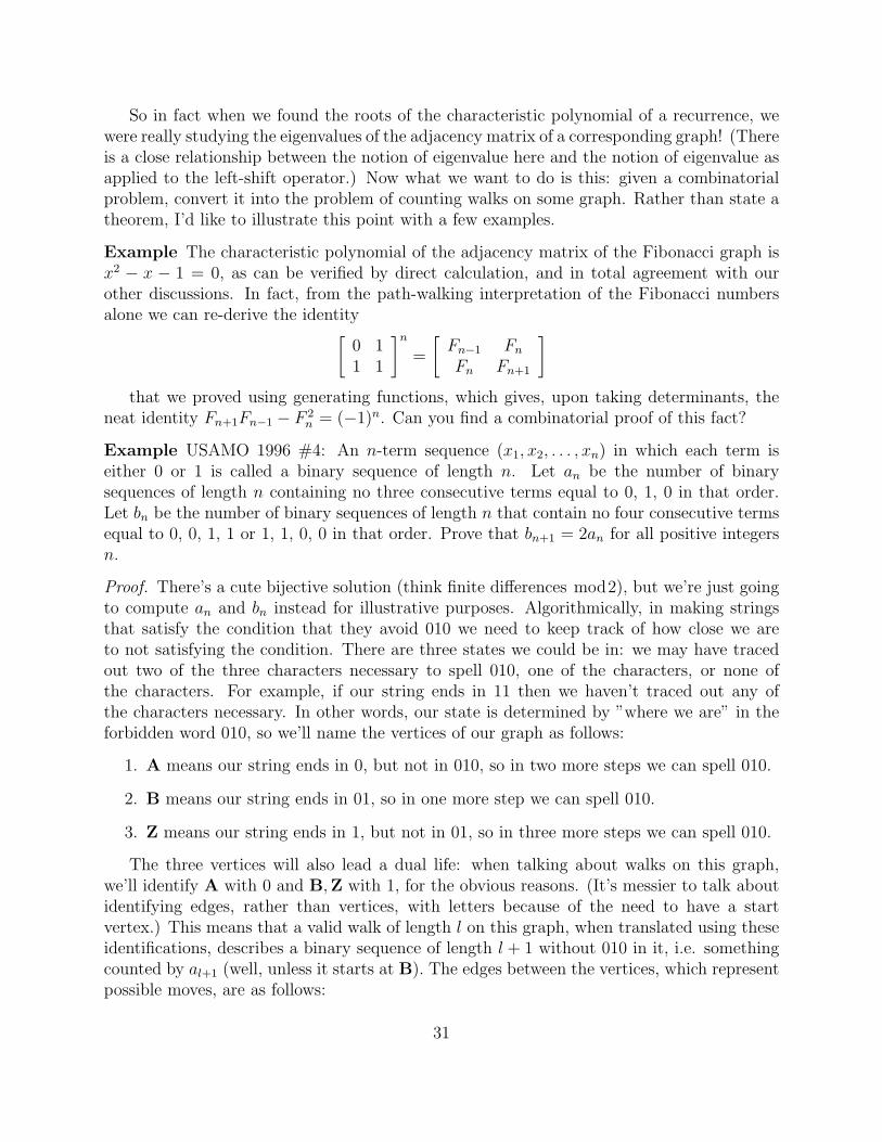
Example USAMO 1996 #4: An n-term sequence (x1, x2, . . . , xn) in which each term iseither 0 or 1 is called a binary sequence of length n. Let an be the number of binarysequences of length n containing no three consecutive terms equal to 0, 1, 0 in that order.Let bn be the number of binary sequences of length n that contain no four consecutive termsequal to 0, 0, 1, 1 or 1, 1, 0, 0 in that order. Prove that bn+1 = 2an for all positive integersn.

Proof. There’s a cute bijective solution (think finite differences mod2), but we’re just goingto compute an and bn instead for illustrative purposes. Algorithmically, in making stringsthat satisfy the condition that they avoid 010 we need to keep track of how close we areto not satisfying the condition. There are three states we could be in: we may have tracedout two of the three characters necessary to spell 010, one of the characters, or none ofthe characters. For example, if our string ends in 11 then we haven’t traced out any ofthe characters necessary. In other words, our state is determined by ”where we are” in theforbidden word 010, so we’ll name the vertices of our graph as follows:

1. A means our string ends in 0, but not in 010, so in two more steps we can spell 010.

2. B means our string ends in 01, so in one more step we can spell 010.

3. Z means our string ends in 1, but not in 01, so in three more steps we can spell 010.

The three vertices will also lead a dual life: when talking about walks on this graph,we’ll identify A with 0 and B,Z with 1, for the obvious reasons. (It’s messier to talk aboutidentifying edges, rather than vertices, with letters because of the need to have a startvertex.) This means that a valid walk of length l on this graph, when translated using theseidentifications, describes a binary sequence of length l + 1 without 010 in it, i.e. somethingcounted by al+1 (well, unless it starts at B). The edges between the vertices, which representpossible moves, are as follows:

31

1. A points to B and itself. If we plop down a 1, we’re at B. If we plop down a 0, we’restill at A.

2. B points to Z. Since we can’t spell 010, the only thing we can do is plop down a 1,and that takes us ”back to the beginning,” i.e. we haven’t spelled out any of 010.

3. Z points to A and itself. If we plop down a 0, we’re at A; otherwise, we’re still ”atthe beginning.”

This gives the following graph:

A B

Z

What we’ve done is essentially performed the Knuth-Morris-Pratt algorithm, which isan algorithm that searches for a string by constructing a finite state machine that measureshow close a given text is to spelling it out at any point. This state machine is very nearlythe directed graph we want to construct to avoid this string; the above example should beenough to get the idea across in lieu of an actual description of the algorithm.

Now, the adjacency matrix of this graph is therefore 1 1 00 0 11 0 1

which has characteristic polynomial Pa(λ) = λ3− 2λ2 + λ− 1. It’s easy to verify that Pa

has no rational roots, but the point is that an is the number of walks starting from either Zor A of length n− 1, so we can write down the recursion

an+3 = 2an+2 − an+1 + an

32

and even compute initial values fairly quickly. What I’d like to emphasize is that theabove procedure is totally algorithmic and hence very general. While it might be possibleto cleverly figure out the above recursion for this particular problem, the KMP algorithmallows us to solve any problem of the type ”count the number of strings on some alphabetthat avoid a particular substring.”

The KMP algorithm doesn’t apply to computing bn because there are now two substringswe want to avoid, but it is not hard to modify: the generalization is called the Aho-Corasickalgorithm, but again rather than describe the algorithm we’ll perform it for bn. The verticesand edges are as follows, with similar reasoning as the reasoning for an:

1. A means the string ends in 0, but not in 110. A points to D and B.

2. B means the string ends in 00, but not in 1100. B points to C and itself.

3. C means the string ends in 001. C points to A.

4. D means the string ends in 1, but not in 001. D points to E and A.

5. E means the string ends in 11, but not in 0011. E points to F and itself.

6. F means the string ends in 110. F points to D.

The graph is as follows:

A B C

D E F

As before, bn is the number of walks of length n−1 starting from A or D. The adjacency

33

matrix of the graph is 0 1 0 1 0 00 1 1 0 0 01 0 0 0 0 01 0 0 0 1 00 0 0 0 1 10 0 0 1 0 0

=

[M NN M

]

where M,N are 3× 3 matrices. Now, it’s not hard to see that we can block-diagonalizeas follows: [

I II −I

]−1 [M NN M

] [I II −I

]=

[M + N 0

0 M−N

]where I is the 3× 3 identity. This block-diagonalization takes advantage of a particular

symmetry of the problem, but the point stands: Aho-Corasick is a totally algorithmic wayof solving problems like this in general. But let’s finish. Since bn is the number of walksstarting from either A or D, it was (before we changed bases) generated by the vector withentries 1, 0, 0, 1, 0, 0 - but this is precisely the first column of the matrix we changed basesby! It follows that the vector we want in the new basis is just 1, 0, 0, 0, 0, 0; that is, bn is thefirst entry in

[M + N 0

0 M−N

]n−1

100000

and hence it is totally determined by the behavior of

M + N =

1 1 00 1 11 0 0

.But this is just a permutation of the adjacency matrix of the graph of an! So in fact an and

bn satisfy the same recursion, and the rest can be proven by checking initial conditions or bywriting down exactly how an and bn are related by permuting the above matrix appropriately.We’ve even been naturally led, in some sense, to the bijective proof: what the above tells usis that certain pairs of points in the graph of bn get sent to certain other pairs in the sameway that points of the graph of an get sent to other points.

34

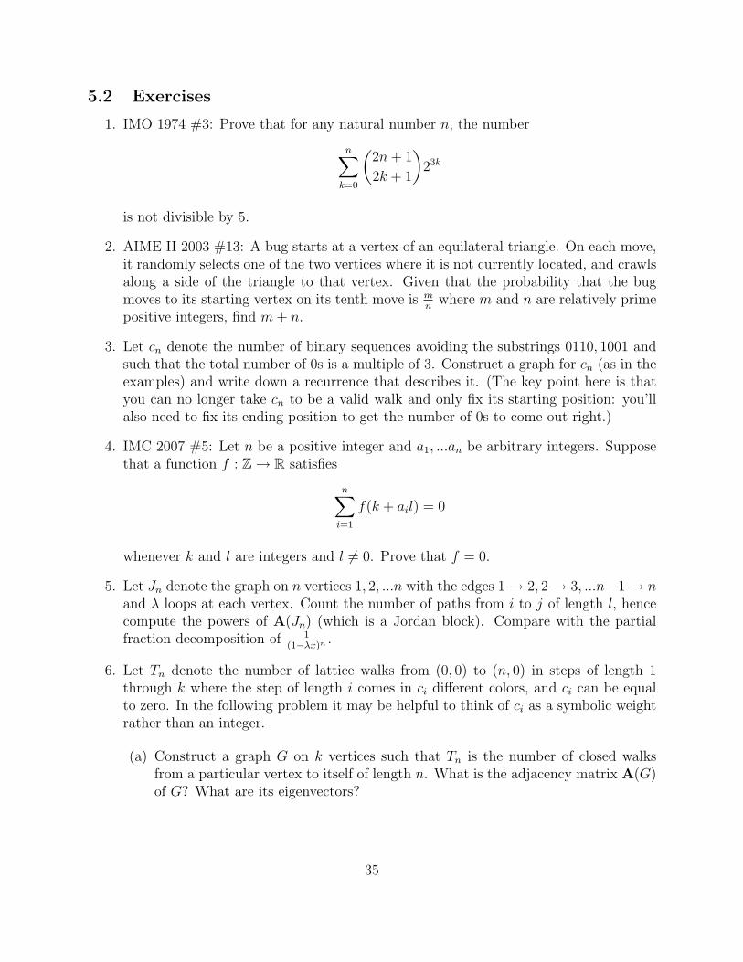
5.2 Exercises

1. IMO 1974 #3: Prove that for any natural number n, the number

n∑k=0

(2n+ 1

2k + 1

)23k

is not divisible by 5.

2. AIME II 2003 #13: A bug starts at a vertex of an equilateral triangle. On each move,it randomly selects one of the two vertices where it is not currently located, and crawlsalong a side of the triangle to that vertex. Given that the probability that the bugmoves to its starting vertex on its tenth move is m

nwhere m and n are relatively prime

positive integers, find m+ n.

3. Let cn denote the number of binary sequences avoiding the substrings 0110, 1001 andsuch that the total number of 0s is a multiple of 3. Construct a graph for cn (as in theexamples) and write down a recurrence that describes it. (The key point here is thatyou can no longer take cn to be a valid walk and only fix its starting position: you’llalso need to fix its ending position to get the number of 0s to come out right.)

4. IMC 2007 #5: Let n be a positive integer and a1, ...an be arbitrary integers. Supposethat a function f : Z→ R satisfies

n∑i=1

f(k + ail) = 0

whenever k and l are integers and l 6= 0. Prove that f = 0.

5. Let Jn denote the graph on n vertices 1, 2, ...n with the edges 1→ 2, 2→ 3, ...n−1→ nand λ loops at each vertex. Count the number of paths from i to j of length l, hencecompute the powers of A(Jn) (which is a Jordan block). Compare with the partialfraction decomposition of 1

(1−λx)n .

6. Let Tn denote the number of lattice walks from (0, 0) to (n, 0) in steps of length 1through k where the step of length i comes in ci different colors, and ci can be equalto zero. In the following problem it may be helpful to think of ci as a symbolic weightrather than an integer.

(a) Construct a graph G on k vertices such that Tn is the number of closed walksfrom a particular vertex to itself of length n. What is the adjacency matrix A(G)of G? What are its eigenvectors?

35

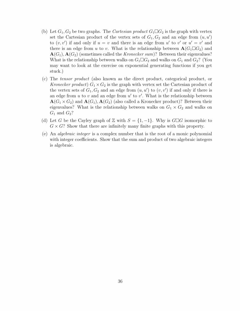
(b) Let G1, G2 be two graphs. The Cartesian product G1�G2 is the graph with vertexset the Cartesian product of the vertex sets of G1, G2 and an edge from (u, u′)to (v, v′) if and only if u = v and there is an edge from u′ to v′ or u′ = v′ andthere is an edge from u to v. What is the relationship between A(G1�G2) andA(G1),A(G2) (sometimes called the Kronecker sum)? Between their eigenvalues?What is the relationship between walks on G1�G2 and walks on G1 and G2? (Youmay want to look at the exercise on exponential generating functions if you getstuck.)

(c) The tensor product (also known as the direct product, categorical product, orKronecker product) G1×G2 is the graph with vertex set the Cartesian product ofthe vertex sets of G1, G2 and an edge from (u, u′) to (v, v′) if and only if there isan edge from u to v and an edge from u′ to v′. What is the relationship betweenA(G1×G2) and A(G1),A(G2) (also called a Kronecker product)? Between theireigenvalues? What is the relationship between walks on G1 × G2 and walks onG1 and G2?

(d) Let G be the Cayley graph of Z with S = {1,−1}. Why is G�G isomorphic toG×G? Show that there are infinitely many finite graphs with this property.

(e) An algebraic integer is a complex number that is the root of a monic polynomialwith integer coefficients. Show that the sum and product of two algebraic integersis algebraic.

36

6 The roots of unity filter

Suppose we have a polynomial or a power series

F (x) =∑n≥0

fnxn

and we’re interested in extracting only the terms with n even or n odd. It’s not hard tosee how to do this by noting that

F (−x) =∑n≥0

fn(−x)n

which, combined with F , allows us to isolate the even and odd terms: in fact, we have∑n≥0

f2nx2n =

F (x) + F (−x)

2

∑n≥0

f2n+1x2n+1 =

F (x)− F (−x)

2.

Probably the most famous example of such an extraction is F (x) = eix. This also offersa pretty easy proof that∑

k≥0

(n

2k

)=∑k≥0

(n

2k + 1

)=

(1 + 1)n ± (1− 1)n

2= 2n−1,

although this is a pretty easy identity to prove combinatorially. Nevertheless, this ideais surprisingly useful.

Example Let Sn = {12, 1

3, ... 1

n} and, given a subset S of Sn, let P (S) denote the product of

all of the elements of S. What is the sum of all such products over all subsets S with aneven number of elements?

Proof. Remove the parity constraint. A moment’s thought reveals that the answer is

n∏k=2

(1 +

1

k

)=n+ 1

2

since the expansion of this product contains every product P (S) exactly once. This is justan expression of the fact that (1 + t1)...(1 + tn) gives the elementary symmetric polynomialsin t1, ...tn. Now, add the parity constraint back in. The sum over all products P (S) with |S|even minus the products with |S| odd is then, after another moment’s thought,

n∏k=2

(1− 1

k

)=

1

n.

Then the answer we want is justn+1

2+ 1n

2= n2+n+2

4n.

37

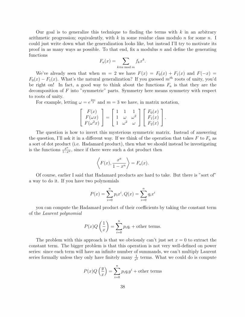
Our goal is to generalize this technique to finding the terms with k in an arbitraryarithmetic progression; equivalently, with k in some residue class modulo n for some n. Icould just write down what the generalization looks like, but instead I’ll try to motivate itsproof in as many ways as possible. To that end, fix a modulus n and define the generatingfunctions

Fa(x) =∑

k≡a mod m

fkxk.

We’ve already seen that when m = 2 we have F (x) = F0(x) + F1(x) and F (−x) =F0(x)− F1(x). What’s the natural generalization? If you guessed mth roots of unity, you’dbe right on! In fact, a good way to think about the functions Fa is that they are thedecomposition of F into ”symmetric” parts. Symmetry here means symmetry with respectto roots of unity.

For example, letting ω = e2πi3 and m = 3 we have, in matrix notation, F (x)

F (ωx)F (ω2x)

=

1 1 11 ω ω2

1 ω2 ω

F0(x)F1(x)F2(x)

.The question is how to invert this mysterious symmetric matrix. Instead of answering

the question, I’ll ask it in a different way. If we think of the operation that takes F to Fa asa sort of dot product (i.e. Hadamard product), then what we should instead be investigatingis the functions xa

1−xn , since if there were such a dot product then⟨F (x),

xa

1− xn

⟩= Fa(x).

Of course, earlier I said that Hadamard products are hard to take. But there is ”sort of”a way to do it. If you have two polynomials

P (x) =n∑i=0

pixi, Q(x) =

n∑i=0

qixi

you can compute the Hadamard product of their coefficients by taking the constant termof the Laurent polynomial

P (x)Q

(1

x

)=

n∑i=0

piqi + other terms.

The problem with this approach is that we obviously can’t just set x = 0 to extract theconstant term. The bigger problem is that this operation is not very well-defined on powerseries: since each term will have an infinite number of summands, we can’t multiply Laurentseries formally unless they only have finitely many 1

xkterms. What we could do is compute

P (x)Q(yx

)=

n∑i=0

piqiyi + other terms

38

but it’s still not clear how to extract the constant term here. If only there were somekind of linear operator that could conveniently remove the other terms...

Depending on how familiar you are with Fourier analysis, you may or may not find thenext step motivated. We’re going to substitute x = eit and integrate away all the terms wedon’t want. More formally, the following is true.

Theorem 6.1. Let A(t) =∑

n∈Z aneint, B(x) =

∑n∈Z bne

int be two Fourier series. Then∑anbn =

1

2π

∫ π

−πA(t)B(t) dt.

This is known as Parseval’s theorem: it implies that the Fourier transform is unitary. Ifyou haven’t seen it before, just remember that the terms einte−int in the product A(t)B(t)integrate to 2π whereas the terms einte−imt,m 6= n integrate to zero. What Parseval’stheorem tells us is that, letting z = eit, A(t) = F (rz) for some r which you can think of asbeing either formal or in the disc |r| < 1, and B(t) = za

1−zn , we obtain

Fa(r) =1

2π

∫ π

−π

F (rz)zn−a

zn − 1dt

=1

2πi

∫ π

−π

F (rz)zn−a−1

zn − 1iz dt

=1

2πi

∮|z|=1

F (rz)zn−a−1

zn − 1dz

where we’ve rewritten the integral from −π to π in x as a contour integral over the circlein z. Those familiar with complex analysis should recognize the Cauchy integral formula asbeing applicable, which says this:

Theorem 6.2. Let D be a disc in C, let C be the boundary of D, and let f be a holomorphicfunction on an open set containing D. Then for every p in the interior of D,

f(p) =1

2πi

∮C

f(z)

z − pdz.

All we have to do now is figure out the partial fraction decomposition of zn−a−1

zn−1. But this

is straightforward: Proposition 5.3 gives

zn−a−1

zn − 1=

n−1∑k=0

ζk(n−a−1)

nζk(n−1)(z − ζk)=

1

n

n∑k=0

ζ−ka

z − ζk

where ζ = e2πin is a primitive nth root of unity. Now, of course, we have all the tools we

39

need because the Cauchy integral formula tells us that

Fa(r) =1

2πi

∮|z|=1

n−1∑k=0

F (rz)ζ−ka

z − ζkdz

=1

n

n−1∑k=0

F (rζk)ζ−ka.

You may be familiar with the a = 0 case - it’s the easiest one to convince yourself of -but the general case has a nice ring to it.

Example Let’s compute the sum ∑k≡a mod m

(n

k

).

For some reason, sums of this type appear on competitions a lot (such as Putnam 1974,which is m = 3, but it’s not worth repeating when we can handle the general case immedi-ately). If we take F (x) = (1 + x)n, then the above is just

Fa(1) =1

m

m−1∑i=0

(1 + ζ i)nζ−ia.

In particular, ∑(n

3k

)=

2n + (−ω)n + (−ω2)n

3.

The m = 3 and m = 4 cases are somewhat special, since the terms 1 + ζ i are themselves(at least multiples of) roots of unity; this stops being true for large m.

To see how this relates to inverting the matrix we wrote down earlier, think about Corol-lary 5.5, which says that if

P (x)

Q(x)=

n−1∑i=0

yiQ′(xi)(x− xi)

then P (xi) = yi∀i. If we write P (x) =∑n−1

i=0 pixi, then writing this condition out produces

a system of linear equations whose matrix is the Vandermonde matrix for x0, ...xn−1. If welet then xi = ζ i and yi = ζ(n−a−1)i, the interpolation is obvious: P (x) = xn−a−1 (andQ(x) = xn − 1). On the other hand, this is exactly the partial fraction decompositionwe just found! And what we have to do to solve this interpolation problem is invert theVandermonde matrix

1 1 1 . . . 11 ζ ζ2 . . . ζn−1

1 ζ2 ζ4 . . . ζ2(n−1)

1 ζ3 ζ6 . . . ζ3(n−1)

......

.... . .

...1 ζn−1 ζ2(n−1) . . . ζ(n−1)(n−1)

40

which is precisely the matrix that relates Fa(x) to F (ζkx). In fact, the result we justderived is equivalent to the rather remarkable statement that the above matrix is unitary(well, after multiplying by 1√

n), i.e. its conjugate transpose is its own inverse. Actually, the

connection goes even deeper: recall that the Fourier coefficients of a function on [−π, π] aredefined by

f̂(n) =1

2π

∫ π

−πf(x)e−inx dx

which gives

f(x) =∑n∈Z

f̂(n)einx

whereas here we have the relationship

Fa =1

n

n−1∑k=0

F (rζk)ζ−ka

that was deduced from the relationship

F (x) =n−1∑k=0

Fa(x)ζa.

Look familiar? If we identify n with 2π, the sum with the integral, and ζ with eix

these formulas are identical! In fact, the relationship between F and Fa is also that of aFourier transform. The unitary matrix that relates F and Fa is called the discrete Fouriertransform matrix of order n, and these two cases are examples of a deeper phenomenoncalled Pontryagin duality. For a survey of the basic results I highly recommend Stein andShakarchi [5].

As promised, I want to motivate what we’re doing here in as many ways as possible.One way to think about what we did is the following: Fa is an n-periodic function in a. Ann-periodic function satisfies the linear recurrence

sn+k = sk∀k

so its characteristic polynomial is xn − 1 and every such function can be written as asum of nth roots of unity raised to the appropriate power. If we’ve solved the problem forthe periodic sequence 1, 0, 0, ...1, 0, 0, ... then we can just shift whatever coefficients we get inthat case to get the coefficients for the other cases, and by linearity we’re done. But observethat the claim that the DFT matrix is unitary is equivalent to the claim that the vectors(ζak) form an orthonormal basis of the space of n-periodic functions (if we define the innerproduct correctly): ⟨

ζak, ζbk⟩

=1

n

n−1∑k=0

ζakζbk =

{1 if a = b

0 otherwise.

41

Some authors don’t put the n in the inner product and instead take the basis to be ζak√n

,but I think this is unnecessary. Orthogonality is a general property of Fourier series, andalthough it is very deep, it’s also very easy to prove in this case: if a 6= b then n can’t dividea− b, so ζ(a−b)k is some multiple of some sum of primitive mth roots of unity for some m|n,and it’s obvious that these will sum to zero. And once we have an orthonormal basis, wealso know how to write any vector in that basis: the coefficient of ζak is

⟨s, ζak

⟩=

1

n

n−1∑k=0

skζ−ak.

And this is the bare-bones of how Fourier analysis on the cyclic group Z/nZ works.Here’s another way to think about these results. If you think of the ζks as being eigen-

values of some adjacency matrix, then the sums we’ve been looking at must count paths onsome graph. And there is a very good candidate for such a graph if we think about whathaving a characteristic polynomial of xn = 1 entails.

Definition Let G be a group and let S be a generating set for G. The Cayley graph of Gwith respect to S is the graph with vertex set G and edges (g, h) if and only if there is s ∈ Ssuch that h = sg. If s ∈ G⇔ s−1 ∈ G, then the edges can be treated as undirected.

Note that if G = Z then we recover the one-dimensional walk with S the set of steps, andif G = Z2 then we recover the two-dimensional walk! Hence our discussion of lattice-pathcounting is really a special case of a more general phenomenon.

The graph we want is the Cayley graph Cn of Z/nZ with S = {1}, otherwise known asa directed cycle. You can think of it as the n-gon that the nth roots of unity trace out inthe complex plane with S = {ζ}. Unlike the other graphs we looked at, this one is easy tovisualize. Counting paths on Cn is very easy. The number of paths of length l from 0 to ais 0 if n 6 |l − a and 1 if n|l − a. This sequence has generating function xa

1−xn ; look familiar?The adjacency matrix of Cn is

0 1 0 0 . . . 00 0 1 0 . . . 00 0 0 1 . . . 00 0 0 0 . . . 0...

......

.... . .

...1 0 0 0 . . . 0

,

which is a cyclic permutation matrix, which we’ll denote P. Powers of this matrix behavein the obvious way, and its eigenvalues are 1, ζ, ...ζn−1, exactly as expected. What are its

42

eigenvectors? Well:

0 1 0 0 . . . 00 0 1 0 . . . 00 0 0 1 . . . 00 0 0 0 . . . 0...

......

.... . .

...1 0 0 0 . . . 0

1ζa

ζ2a

ζ3a

...ζ(n−1)a

= ζa

1ζa

ζ2a

ζ3a

...ζ(n−1)a

so we have the following beautiful result: the discrete Fourier transform matrix diago-

nalizes cyclic permutations! (One of the exercises considers a generalization of this result.)If you like, you can think of these eigenvectors as the ”harmonics” of the n-gon. Now count-ing paths by diagonalizing gets us orthogonality, the same as before, as well as the partialfraction decomposition of xa

1−xn .Actually, we don’t even need to count paths: instead, we can take S = {1,−1} and

construct the undirected cycle UCn, which is like the directed cycle but, well, undirected.The adjacency matrix of the undirected cycle is

0 1 0 0 . . . 11 0 1 0 . . . 00 1 0 1 . . . 00 0 1 0 . . . 0...

......

.... . .

...1 0 0 0 . . . 0

which is P+Pn−1. Since P commutes with itself, it follows that the eigenvectors haven’t

changed and the eigenvalues are of the form ζ + ζn−1 = 2 cos 2πian

, which are real sincethe adjacency matrix is symmetric. But now we get orthogonality as a consequence of thespectral theorem.

Counting paths on UCn is quite interesting: you can think of it as a finite approximationto counting paths on Z, and so it becomes natural to think about, for example, the closedpaths of length 2l from 0 to 0. (If n is even, there are no closed paths of odd length, so thisquestion will be easier to answer.) As the number of vertices n gets large, if our intuition iscorrect we should expect this number to be asymptotic to

(2ll

), the number of ways to walk

2l steps in one dimension and get back to the origin. To show that this is the case, we’ll usethe following lemma.

Lemma 6.3. Let A be an adjacency matrix of a graph. The total number of closed paths oflength l is tr(Al).

This is by definition; that’s exactly what the sum of the diagonal elements are. But wecan take advantage of the fact that the trace of a matrix is also the sum of its eigenvalues,and since the graph we’re looking at has this nice rotational symmetry, to find the number

43

of closed paths from a particular vertex to itself we just have to divide by n, so we want tocompute

1

n

n−1∑k=0

(2 cos

2πk

n

)2l

=1

n

n−1∑k=0

(ζk + ζ−k)2l

=1

n

n−1∑k=0

2l∑i=0

(2l

i

)ζk(2i−2l)

=2l∑i=0

(2l

i

)1

n

n−1∑k=0

ζk(2i−2l).

But we know how to compute sums like these; the sum over all k will just be zero unless2i− 2l ≡ 0 mod n. Hence this sum will be equal to∑

2i≡2l mod n

(2l

i

).

This is definitely the correct answer from a combinatorial standpoint: we’re just countingwalks from (0, 0) to (2l, 2i − l) for some i such that 2i ≡ 2l mod n. Note that, exactly asexpected, if l < n then

(2ll

)is the lone term, since if we haven’t walked more than l steps then

our graph is indistinguishable from Z. Here’s the fun part: if we take the limit as n → ∞,the above sum becomes a Riemann sum and hence an integral: in fact, we have∫ 1

0

(2 cos 2πx)2l dx =

(2l

l

).

Thus in some sense 2 cos 2πx, x ∈ [0, 1) is an infinite set of eigenvalues, or spectrum, forthe Cayley graph of Z. We are also led to the philosophy that Fourier analysis on the circleis in some sense a ”limit” of Fourier analysis on Z/nZ as n is taken to infinity.

I’d like to end with a nontrivial application.

Example Suppose that the non-negative integers are written as a disjoint union of a finitenumber of arithmetic progressions with common differences d1 ≥ d2 ≥ ... ≥ dn ≥ 1. Provethat d1 = d2.

Proof. The generating functions proof is more or less obvious: this is possible if and only if

1

1− x=

n∑k=1

xak

1− xdk

where the arithmetic progression with common difference dk has initial term ak. If d1 >d2, then the partial fraction decomposition of the RHS has terms involving dth1 roots of unitythat don’t cancel with any of the other terms.

44

But there’s a philosophy behind this solution that is worth thinking about. Subsets of theintegers can be identified with their indicator functions, which is the function on Z that is 0if an element isn’t in the set and 1 if it is. And indicator functions have Fourier coefficients:in particular, large Fourier coefficients imply correlation with an arithmetic progression.This is a surprisingly powerful idea and has found some highly nontrivial applications incombinatorics, for example in the proof of Roth’s theorem.

What it means for us is that there is a very nice interpretation of what we’ve done: let Sbe a disjoint union of a finite number of arithmetic differences. If d1 > d2, then the Fouriercoefficients of period d1 of the indicator function of S are nonzero. On the other hand, theindicator function of the non-negative integers is the constant function, so all of its Fouriercoefficients are zero.

45

6.1 Exercises

1. Putnam 1983 A4: Let k be a positive integer and let m = 6k − 1. Let

S(m) =2k−1∑j=1

(−1)j+1

(m

3j − 1

).

Prove that S(m) is never zero.

2. Putnam 1985 A6: If p(x) = a0 + a1x+ ...+ amxm is a polynomial with real coefficients

ai, then setΓ(p(x)) = a2

0 + a21 + ...+ a2

m.

Let F (x) = 3x2 + 7x + 2. Find, with proof, a polynomial g(x) with real coefficientssuch that g(0) = 1 and Γ(f(x)n) = Γ(g(x)n) for every integer n ≥ 1.

3. Let Vn,m = span{(a1x1+a2x2+...+anxn)m|(a1, ...an) ∈ Cn} considered as a subspace ofC[x1, ...xn]. Show that it contains every monomial xλ1

1 xλ22 ...x

λnn where λ1 + ...+λn = m,

i.e. it is as large as it can be.

4. Let Un(y) denote the characteristic polynomial of the adjacency matrix of UCn, withthe conventions U0(y) = 1, U1(y) = y. Compute

∞∑n=0

Un(y)xn.

What are the roots of Un(y)?

5. An n × n matrix is called circulant if its entries aij are a function of the value ofi− j mod n.

(a) Show that every circulant matrix is a sum of powers of the cyclic permutationmatrix P. Hence show that every circulant matrix is diagonalized by the DFTmatrix. Conclude that the product of two circulant matrices is circulant and thecirculant matrices form an algebra.

(b) IMO 1979 #6: Let A and E be opposite vertices of an octagon. A frog starts atvertex A. From any vertex except E it jumps to one of the two adjacent vertices.When it reaches E it stops. Let an be the number of distinct paths of exactly njumps ending at E. Prove that

a2n−1 = 0, a2n =(2 +

√2)n−1 − (2−

√2)n−1

√2

.

46

(c) Putnam 1985 B5: Let Mn be the (2n+ 1)× (2n+ 1) for which

(Mn)ij =

0 if i = j

1 if i− j ≡ 1, 2, ...n mod (2n+ 1)

−1 if i− j ≡ n+ 1, ...2n mod (2n+ 1).

Find the rank of Mn.

(d) Construct a graph on m vertices 0, 1, 2, ...m− 1 such that the number of walks oflength l from 0 to a is ∑

k≡a mod m

(l

k

).

More generally, what kind of graphs have circulant adjacency matrices?

6. Let G = (Z/2Z)n be the abelian group consisting of all n-tuples of 0s and 1s undercomponentwise addition mod2.

(a) Describe the Fourier transform on G: in other words, given a function f : G →R (we don’t need all of C), decompose it into a sum of homomorphisms, orcharacters, of G, which are functions χu : G→ R such that

χu(ab) = χu(a)χu(b)

and1

2n

∑g∈G

χu(g)χv(g) =

{1 if u = v

0 otherwise.

(b) Let S be the set of all elements of G with exactly one 1. What familiar geometricshape is the Cayley graph (G,S)? What are the eigenvalues and eigenvectors ofits adjacency matrix?

(c) IMO 2008 #5: Let n and k be positive integers with k ≥ n and k − n an evennumber. Let 2n lamps labelled 1, 2, ..., 2n be given, each of which can be eitheron or off. Initially all the lamps are off. We consider sequences of steps: at eachstep one of the lamps is switched (from on to off or from off to on).

Let N be the number of such sequences consisting of k steps and resulting in thestate where lamps 1 through n are all on, and lamps n+ 1 through 2n are all off.

Let M be number of such sequences consisting of k steps, resulting in the statewhere lamps 1 through n are all on, and lamps n + 1 through 2n are all off, butwhere none of the lamps n+ 1 through 2n is ever switched on.

Determine NM

.

47

7 Additional exercises

The following problems don’t fit neatly into the above categories, but you should find yourselfwell-prepared to tackle them anyway!

1. Let f(x) = a0 + a1x + ... be a power series with integer coefficients, with a0 6= 0.

Suppose that the power series expansion of f ′(x)f(x)

at x = 0 also has integer coefficients.

Prove or disprove that a0|an for all n ≥ 0.

2. Putnam 1999 B3: Let A = {(x, y) : 0 ≤ x, y < 1}. For (x, y) ∈ A, let

S(x, y) =∑

12≤mn≤2

xmyn

where m,n are positive integers. Evaluate

lim(x,y)→(1,1),(x,y)∈A

(1− xy2)(1− x2)S(x, y).

3. (a) Let p be a prime. Show that (x+ 1)p ≡ xp + 1 mod p.

(b) Let m,n be positive integers with base p representations

m = mkpk +mk−1p

k−1 + ...+m0

n = nkpk + nk−1p

k−1 + ...+ n0.

Prove Lucas’ theorem: (m

n

)≡

k∏i=0

(mi

ni

)mod p.

(c) Putnam 1983 A3: Let p be an odd prime and let

F (n) = 1 + 2n+ 3n2 + ...+ (p− 1)np−2.

Prove that if a 6≡ b mod p then F (a) 6≡ F (b) mod p.

(d) IMO Shortlist 1988 #2: Let n be a positive integer. Find the number of oddcoefficients in

un(x) = (x2 + x+ 1)n.

4. Let p be a prime and let vp(n) denote the greatest power of p that divides n. Let sp(n)denote the sum of the digits of n in base p.

(a) Show that

vp(n!) =n− sp(n)

p− 1.

Prove Kummer’s theorem: vp((mn

))is the number of carries required to add n

and n−m in base p.

48

(b) Compute ∑n≥0

sp(n)xn.

5. Let T (n) denote the number of non-congruent non-degenerate triangles with integerside lengths adding up to n. For example, T (3) = 1. Show that∑

n≥0

T (n)xn =q3

(1− q2)(1− q3)(1− q4).

6. The exponential generating function of a sequence an is given by

Ea(x) =∑n≥0

anxn

n!.

(a) Show that EaEb = Ec, where

cn =n∑k=0

(n

k

)akbn−k =

∑S,T

a|S|b|T |

where S, T range over disjoint subsets of some n-element set.

(b) Suppose an, bn are sequences such that an =∑n

k=0

(nk

)bk. Show that

bn =n∑k=0

(−1)n−k(n

k

)ak.

Interpret this result in terms of Cartesian products of graphs.

(c) Show that the exponential generating function of a sequence satisfying a linearhomogeneous recurrence satisfies a linear homogeneous ordinary differential equa-tion.

(d) The Bell numbers Bn count the number of partitions of the set {1, 2, 3, ...n}, whereneither the order of the partitions nor the order of the elements of the partitionsmatter. Show that

Bn+1 =n∑k=0

(n

k

)Bk

and hence compute∑

n≥0Bnxn

n!.

(e) Let In denote the number of permutations of n elements which have order 2. Showthat

In+1 = In + nIn−1

and hence compute∑

n≥0 Inxn

n!.

49

(f) Prove the fundamental theorem of exponential generating functions : given a se-quence f(n), define h(0) = 1 and

h(|S|) =∑k≥0

∑B

f(|B1|)...f(|Bk|)

where B1, ...Bk range over all partitions of S into disjoint subsets. Show thatEh = exp(Ef ). Use this result to give a second proof of the result of the previousproblem. What about the number of permutations with order 3?

(g) IMO 1987 #1: Let pn(k) be the number of permutations of {1, 2, ...n} which haveexactly k fixed points. Prove that

n∑k=1

kpn(k) = n!.

(h) Putnam 2005 B6: Let Sn denote the set of all permutations of {1, 2, ...n}. Forπ ∈ Sn, let σ(π) = 1 if π is an even permutation and−1 if π is an odd permutation.Also, let ν(π) denote the number of fixed points of π. Show that∑

π∈Sn

σ(π)

ν(π) + 1= (−1)n+1 n

n+ 1.

(A permutation is called even or odd if it can be written as a product of, re-spectively, an even or odd number of transpositions. Equivalently, σ(π) is thedeterminant of the permutation matrix associated to π.)

7. Given a function a(n) : N→ C, define its Dirichlet generating function

L(s, a) =∑n≥1

a(n)

ns.

where s ∈ C.

(a) Suppose a(n) is multiplicative, i.e. a(mn) = a(m)a(n) if gcd(m,n) = 1. Showthat

L(s, a) =∏

p is prime

∑k≥0

a(pk)

pks,

i.e. L has an Euler product. Show a similar result in the case that a(n) is totallymultiplicative (the gcd assumption can be dropped), hence the case that a(n) = 1(the Riemann zeta function).

50

(b) Show that the a(n) = 1 Euler product implies that∑p is prime

1

p

diverges. Conclude that there are infinitely many primes and, moreover, thatthere does not exist a finite collection of polynomials of degree 2 or greater suchthat their values at the integers contain the primes.

(c) Show that L(s, a)L(s, b) = L(s, c), where

c(n) =∏d|n

a(n)b(nd

)is the Dirichlet convolution of a and b, to be written a ∗ b. Conclude that theDirichlet convolution of two multiplicative functions is multiplicative.

(d) Show that the totient function ϕ(n), the divisor function d(n), and the Mobiusfunction µ(n) (which is equal to 1 if n is a product of an even number of distinctprimes, −1 if n is a product of an odd number of distinct primes, and 0 otherwise)are multiplicative. Compute their Dirichlet generating functions.

(e) Prove Mobius inversion: b = a ∗ 1 if and only if a = b ∗ µ.

(f) Let a necklace of length l be a string of l beads that can be one of n colors, withthe equivalence relation that two necklaces are the same if one can be obtainedfrom the other by cyclic permutation. Compute the number of distinct necklacesof length l.

(g) For a given modulus m, define a Dirichlet character with respect to m to be afunction χ : N→ C such that χ(n) = 0 if (n,m) > 1, χ(n) = χ(n+m), and χ isa homomorphism from (Z/mZ)∗ to C, i.e. it is a group character of Z/ϕ(m)/Z.Among other things, this implies that χ is totally multiplicative. For m = 3, 4,use the values of L(s, χ) as χ ranges over all characters to show that∑

p is prime,p≡a mod m

1

p

diverges, where gcd(a,m) = 1. (The proof is substantially harder for general m;the result is known as Dirichlet’s theorem.)

(h) Let r2(n) denote the number of ways n can be written as a sum of two squares,where order and sign are both taken into account, and let χ(n) be the Dirichletcharacter with respect to 4 given by χ(3) = −1. Show that

r2(n) =∑d|n

χ(d).

51

8. Given a semigroup G (a group which is not required to have inverses or an identity),its semigroup algebra C[G] is the algebra of formal linear combinations of elements ofG with multiplication given by the semigroup operation, i.e. g(ah1 + bh2) = a(gh1) +b(gh2) where a, b ∈ C and g, h1, h2 ∈ C. If G is a group, C[G] is called the groupalgebra and is also known as the regular representation of G.

(a) Show that the algebra of ordinary generating functions in n variables is (isomor-phic to) the semigroup algebra of the free semigroup on n generators, i.e. forn = 1 the non-negative integers under addition. Also show that the algebra ofDirichlet generating functions is (isomorphic to) the semigroup algebra of thepositive integers under multiplication.

(b) Show that the algebra of n × n circulant matrices is (isomorphic to) the groupalgebra of Z/nZ, hence to C[x]/(xn − 1). More generally, show how to get aCayley graph out of an element of a group algebra. Hence rework the last exercisein the last section by figuring out an easy way to write down the group algebraof (Z/2Z)n.

(c) Show that if G is a finite abelian group, C[G] has a basis in which all of itselements, considered as linear operators on C[G], are diagonal. Describe theFourier transform on G.

52

References

[1] F. Bergeron, G. Labelle, P. Leroux. Combinatorial Species and Tree-like Structures.Cambridge University Press, 1998.

[2] G. C. Rota. Finite Operator Calculus. Academic Press, Inc., 1975.

[3] R. Stanley. Enumerative Combinatorics, vol. I. Monterey: Wadsworth andBrooks/Cole, 1987.

[4] R. Stanley. Enumerative Combinatorics, vol. II. Cambridge University Press, 2001.

[5] E. M. Stein, R. Shakarchi. Fourier Analysis: an Introduction. Princeton UniversityPress, Princeton, NJ, 2003.

[6] H. Wilf. Generatingfunctionology. Academic Press, Inc., 1994.http://www.math.upenn.edu/ wilf/DownldGF.html.

53