topic nine serial correlation bsc (hons) finance ii/ bsc (hons) finance with law ii module:...

Topic Nine Serial Correlation

BSc (Hons) Finance II/ BSc (Hons) Finance with Law II

Module: Principles of Financial Econometrics I

Lecturer: Dr Baboo M Nowbutsing

Topic 10: Autocorrelation


Outline 1. Introduction 2. Causes of Autocorrelation 3. OLS Estimation 4. BLUE Estimator5. Consequences of using OLS 6. Detecting Autocorrelation


1. Introduction

Autocorrelation occurs in time-series studies when the errors associated with a given time period carry over into future time periods.

For example, if we are predicting the growth of stock dividends, an overestimate in one year is likely to lead to overestimates in succeeding years.


1. Introduction

Times series data follow a natural ordering over time.

It is likely that such data exhibit intercorrelation, especially if the time interval between successive observations is short, such as weeks or days.


1. Introduction

We expect stock market prices to move or move down for several days in succession.

In situation like this, the assumption of no auto or serial correlation in the error term that underlies the CLRM will be violated.

We experience autocorrelation when

0)( jiuuE


1. Introduction

Sometimes the term autocorrelation is used interchangeably.

However, some authors prefer to distinguish between them.

For example, Tintner defines autocorrelation as ‘lag correlation of a given series within itself, lagged by a number of times units’ whereas serial correlation is the ‘lag correlation between two different series’.

We will use both term simultaneously in this lecture.


1. Introduction

There are different types of serial correlation. With first-order serial correlation, errors in one time period are correlated directly with errors in the ensuing time period.

With positive serial correlation, errors in one time period are positively correlated with errors in the next time period.


2. Causes of Autocorrelation

1. Inertia - Macroeconomics data experience cycles/business cycles.

2. Specification Bias- Excluded variable Appropriate equation:

Estimated equation

Estimating the second equation implies

ttttt uXXXY 4433221

tttt vXXY 33221

ttt uXv 44



3. Specification Bias- Incorrect Functional Form

tttt vXXY 223221

ttt uXY 221

ttt vXu 223



4. Cobweb Phenomenon In agricultural market, the supply reacts to

price with a lag of one time period because supply decisions take time to implement. This is known as the cobweb phenomenon.

Thus, at the beginning of this year’s planting of crops, farmers are influenced by the price prevailing last year.



5. Lags

The above equation is known as autoregression because one of the explanatory variables is the lagged value of the dependent variable.

If you neglect the lagged the resulting error term will reflect a systematic pattern due to the influence of lagged consumption on current consumption.

ttt unConsumptionConsumptio 121



6. Data Manipulation

This equation is known as the first difference form and dynamic regression model. The previous equation is known as the level form.

Note that the error term in the first equation is not autocorrelated but it can be shown that the error term in the first difference form is autocorrelated.

ttt uXY 21 11211 ttt uXY

ttt vXY 2



6. Nonstationarity When dealing with time series data, we

should check whether the given time series is stationary.

A time series is stationary if its characteristics (e.g. mean, variance and covariance) are time variant; that is, they do not change over time.

If that is not the case, we have a nonstationary time series.


3. OLS Estimation

Assume that the error term can be modeled as follows:

is known as the coefficient of autocovariance and the error term satisfies the OLS assumption.

This Scheme is known as an Autoregressive (AR(1))process

ttt uXY 21 0)( jiuuE

ttt uu 1 1 1


3. OLS Estimation

2

22

1)()(

tt uEuVar

2

2

1)(),(

ssttstt uuEuuCov

sstt uuCor ),(

21 1 12 1

2 2 2 2ˆ( ) 1 2 2 .... 2t t t t t tn

tt t t t

x x x x x xVar

x x x x


4. BLUE Estimator

Under the AR (1) process, the BLUE estimator of β2 is given by the following expression.

Cxx

yyxxn

t tt

tt

n

t ttGLS

2

2 1

12 1

2)(

))((ˆ

Dxx

Varn

t tt

GLS

2

2 1

2

2)(

)ˆ(


4. BLUE Estimator

The Gauss Theorem provides only the sufficient condition for OLS to be BLUE.

The necessary conditions for OLS to be BLUE are given by Krushkal’s theorem.

Therefore, in some cases, it can happen that OLS is BLUE despite autocorrelation. But such cases are very rare.


5. Consequences of Using OLS

OLS Estimation Allowing for Autocorrelation As noted, the estimator is no more not BLUE,

and even if we use the variance, the confidence intervals derived from there are likely to be wider than those based on the GLS procedure.

Hypothesis testing: we are likely to declare a coefficient statistically insignificant even though in fact it may be.

One should use GLS and not OLS.


5. Consequences of Using OLS

OLS Estimation Disregarding Autocorrelation

The estimated variance of the error is likely to overestimate the true variance

Over estimate R-square Therefore, the usual t and F tests of significance are

no longer valid, and if applied, are likely to give seriously misleading conclusions about the statistical significance of the estimated regression coefficients.


5. Detecting Autocorrelation

Graphical Method There are various ways of examining the residuals. The time sequence plot can be produced. Alternatively, we can plot the standardized residuals

against time. The standardized residuals is simply the residuals

divided by the standard error of the regression. If the actual and standard plot shows a pattern, then

the errors may not be random. We can also plot the error term with its first lag.



The Runs Test- Consider a list of estimated error term, the errors term can be positive or negative. In the following sequence, there are three runs.

(─ ─ ─ ─ ─ ─ ) ( + + + + + + + + + + + + + ) (─ ─ ─ ─ ─ ─ ─ ─ ─ ─ ─ )

A run is defined as uninterrupted sequence of one symbol or attribute, such as + or -.

The length of the run is defined as the number of element in it. The above sequence as three runs, the first run is 6 minuses, the second one has 13 pluses and the last one has 11 runs.



Define N: total number of observations N1: number of + symbols (i.e. + residuals)

N2: number of ─ symbols (i.e. ─ residuals)

R: number of runs Assuming that the N1 >10 and N2 >10, then

the number of runs is normally distributed with:



Then,

If the null hypothesis of randomness is sustainable, following the properties of the normal distribution, we should expect that

Prob [E(R) – 1.96 R ≤ R ≤ E(R) – 1.96 R]

Hypothesis: do not reject the null hypothesis of randomness with 95% confidence if R, the number of runs, lies in the preceding confidence interval; reject otherwise

12

)( 21 N

NNRE

)1()(

)2(22

21212

NN

NNNNNR



The Durbin Watson Test

It is simply the ratio of the sum of squared differences in successive residuals to the RSS.

The number of observation is n-1 as one observation is lost in taking successive differences.

nt

tt

nt

ttt

u

uu

d

1

2

2

21

ˆ

)ˆˆ(



A great advantage of the Durbin Watson test is that based on the estimated residuals. It is based on the following assumptions:

1. The regression model includes the intercept term.

2. The explanatory variables are nonstochastic, or fixed in repeated sampling.

3. The disturbances are generated by the first order autoregressive scheme.



4. The error term is assumed to be normally distributed.

5. The regression model does not include the lagged values of the dependent an explanatory variables.

6. There are no missing values in the data. Durbin-Watson have derived a lower bound dL and

an upper bound dU such that if the computed d lies outside these critical values, a decision can be made regarding the presence of positive or negative serial correlation.



Where

But since -1 ≤ ≤ 1, this implies that 0 ≤ d ≤ 4.

2

1

2

12

12

ˆ

ˆˆ12

ˆ

ˆˆ2ˆˆ

t

tt

t

tttt

u

uu

u

uuuud

12 d

2

1

ˆ

ˆˆˆ

t

tt

u

uu



If the statistic lies near the value 2, there is no serial correlation.

But if the statistic lies in the vicinity of 0, there is positive serial correlation.

The closer the d is to zero, the greater the evidence of positive serial correlation.

If it lies in the vicinity of 4, there is evidence of negative serial correlation



If it lies between dL and dU / 4 –dL and 4 – dU, then we are in the zone of indecision.

The mechanics of the Durbin-Watson test are as follows:

Run the OLS regression and obtain the residuals Compute d For the given sample size and given number of

explanatory variables, find out the critical dL and dU.

Follow the decisions rule



Use Modified d test if d lies in the zone in the of indecision. Given the level of significance ,

Ho: = 0 versus H1: > 0, reject Ho at level if d < dU. That is there is statistically significant evidence of positive autocorrelation.

Ho : = 0 versus H1 : < 0, reject Ho at level if 4- d < dU. That is there is statistically significant evidence of negative autocorrelation.

Ho : = 0 versus H1 : ≠ 0, reject Ho at 2 level if d < dU and 4- d < dU. That is there is statistically significant evidence of either positive or negative autocorrelation.



The Breusch – Godfrey The BG test, also known as the LM test, is a general

test for autocorrelation in the sense that it allows for

1. nonstochastic regressors such as the lagged values of the regressand;

2. higher-order autoregressive schemes such as AR(1), AR (2)etc.; and

3. simple or higher-order moving averages of white noise error terms.



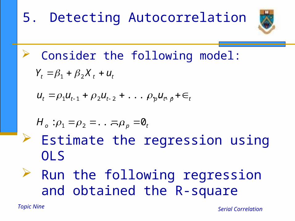
Consider the following model:

Estimate the regression using OLS Run the following regression and obtained the

R-square

ttt uXY 21

tptpttt uuuu ........2211

tpoH 0.....: 21



If the sample size is large, Breusch and Godfrey have shown that (n – p) R2 follow a chi-square

If (n – p) R2 exceeds the critical value at the chosen level of significance, we reject the null hypothesis, in which case at least one rho is statistically different from zero.



Point to note: The regressors included in the regression model may

contain lagged values of the regressand Y. In DW, this is not allowed.

The BG test is applicable even if the disturbances follow a pth-order moving averages (MA) process, that is ut is integrated as follows:

A drawback of the BG test is that the value of p, the length of the lag cannot be specified as a priori.

ptpttttu ........2211



Model Misspecification vs. Pure Autocorrelation

It is important to find out whether autocorrelation is pure autocorrelation and not the result of mis-specification of the model.

Suppose that the Durbin Watson test of a given regression model (wage-productivity) reveals a value of 0.1229. This indicates positive autocorrelation



However, could this correlation have arisen because the model was not correctly specified?

Time series model do exhibit trend, so add a trend variable in the equation.



The Method of GLS

There are two cases when (1) is known and (2) is not known

ttt uXY 21 ttt uu 11 11



When is known If the regression holds at time t, it should hold at

time t-1, i.e.

Multiplying the second equation by gives

Subtracting (3) from (1) gives

11211 ttt uXY

11211 ttt uXY

)()1( 1211 tttt XXpYY

)( 1 ttt uu



The equation can be

The error term satisfies all the OLS assumptions Thus we can apply OLS to the transformed variables

Y* and X* and obtain estimation with all the optimum properties, namely BLUE

In effect, running this equation is the same as using the GLS.

ttttt XY ****



When is unknown, there are many ways to estimate it.

Assume that = +1 the generalized difference equation reduces to the first difference equation

)()( 112 tttttt uuXXYY

ttt XY 2



The first difference transformation may be appropriate if the coefficient of autocorrelation is very high, say in excess of 0.8, or the Durbin-Watson d is quite low.

Maddala has proposed this rough rule of thumb:

Use the first difference form whenever d< R2.



There are many interesting features of the first difference equation

There is no intercept regression in it. Thus, you have to use the regression through the origin routine

If however by mistake one includes an intercept term, then the original model has a trend in it.

Thus, by including the intercept, one is testing the presence of a trend in the equation.



Another interesting feature relates to the stationarity property.

When =1, the error term, ut, is nonstationary, for the variances and covariances become infinite.

When =1, the first differenced ut becomes stationary, as it is equal to q white noise error term.



Based on Durbin-Watson d statistic From the Durbin – Watson Statistics, we

know that

In reasonably large samples one samples one can obtain rho from this equation and use it to transform the data as shown in the GLS.

21

d



Based on the error terms

Estimate the following equation

ttt uu 11

ttt vuu 1ˆ.ˆˆ



Iterative Procedure - We can estimate rho by successive approximation,

starting with some initial value of rho. the Cochran-Orcutt iterative procedure, the Cochran-

Orcutt two-step procedure, the Durbin-Watson two-step procedure and the Hildreth-Lu scanning or search procedure.

The most popular one is the Cochran-Orcutt iterative procedure.

topic nine serial correlation bsc (hons) finance ii/ bsc (hons) finance with law ii module:...

Documents

order serial correlation

positive serial correlation

autocorrelation slide

lag correlation

introduction autocorrelation

causes of autocorrelation

term autocorrelation

nowbutsing topic