topic modeling: proof to practice - microsoft.com · input: term-doc matrix topic 1: identified...

Topic Modeling: Proof to Practice

MSR India . . . . . . . . . . .Bing Ads . . . . . . . . . . . .Indian Institute of Science . . . . . . .

Ravi Kannan, Harsha SimhadriKushal Dave, Shrutendra Harsola

Chiranjib Bhattacharyya

Non-Negative Matrix Factorization

OutputInput

≥ 0 ≥ 0

≥ 0

Topic Modeling

▪𝒏 (106 +) documents. Doc is a 𝒅(5K+) vector of word frequencies.

▪ Assume there are 𝒌 (100s) unknown topics (topic is also a 𝑑-vector) so that each doc is approximately a convex combination of topics.

▪ Find Topics. Too hard in general. Assume Generative Model.

▪ Latent Dirichlet Allocation (LDA) Model [Blei, Ng, Jordan]. For each doc:▪ (Randomly) Generate k-vector of topic weights; take weighted combination of

topics as word-probabilities-vector.

▪ Generate words independently with these probabilities

▪Nice theory. Many applications. But..

INPUT: Term-Doc Matrix

Topic 1: Identified with ``Election’’, ``Putin’’ and ``Debate’’. We can call it ``Politics’’ (ex post facto).Topic 3: ``Weather’’ or ``Seattle’’.Doc 1 ≈ 0.3 (Topic 1) + 0.4 (Topic 2) + 0.3 (Topic 3) = (0.114, 0.084, 0.081, … )

(Latent) Stochastic Model: Has Topic Matrix. Generates topic weights (.3,.4,.3). Generates say 100 words as per 0.114, 0.084, 0.081, … .Out: Only freq of words generated.

OUTPUT : Topics Matrix

ML and Theory

▪Machine Learning has long (since 1990’s) studied these problems.

▪ML: Generative Models. Simple Heuristics. Empirical results.

▪ Theory: developed provable algorithms. Here- ``best of both’’: ▪ Empirically verifiable assumptions.

▪ Good provable time and error bounds.

▪ Scales up on real data (to 100M docs, 6B tokens, 1000 topics on a single box)

▪ Provable: ▪ If data was generated (by unknown model), alg should provably (approx) find

the generating model (Reconstruction).

▪ Prove (good) poly time bounds (for every model satisfying assumptions)

Provable Algorithms for Topic Models, NMF

▪ Arora, Ge, Kannan, Moitra: Provable alg for NMF with assumptions. (STOC 2012).

▪ Arora, Ge, Moitra: Ditto for Topic Modeling. Assumptions.(ICML 2013).

▪ Anandakumar, Foster, Hsu, Kakade: Tensor-based methods (2012)

▪ Bansal, Bhattacharyya, Kannan: Provable Topic Modeling Algorithm under realistic, empirically verified assumptions. (NIPS 2014).

▪ Proof of the pudding: Scalable. Billions of tokens.

▪ Metrics for Real Data (generating model not available).

Given docs (o’s), find 𝑴

Helps to find nearly pure documents (o’s near corners).

x o

Geometry of Topic Modeling: Basic Topics in space spanned by vocabulary

𝑴.,𝟏 = (0.38, 0.28, 0.27, 0, 0, 0, 0, 0.03, 0.01, 0.02, 0.01)

𝑴.,𝟐= (0, 0, 0, 0.38, 0.6, 0, 0, 0, 0.02, 0, 0)𝑴.,𝟑

x o

ox

o x

x o

x o 𝑴.,𝒍 ∶ 𝑙-th topic vector

x : Probability Vector of each doc

= Weighted combination of 𝑀𝑙(𝑷 = 𝑴𝑾 : all probabilities)

o : Observation, i.e., generated doc

(𝑨 : all observations)xo

o x

x o

x o

Dependent Topics

• Existing Models- assume the topic vectors are linearly (``very’’) independent.

• If true, we want to scale upto 5K topics, (essential) rank of data matrix must be 5K. Lets Check! Rank of Data: Observable.

• Real data has rank <<5K! How then can be scale up number of topics?

• Must have linearly dependent topics.

• Our Model: Small number of lin indep basic topics. • Each (actual) topic is a convex combination of two basic topics.

Squared singular values of data matrix

PubMedNY Times

σk2(A)

k

σk2(A)

k

Geometry of Topic Modeling: Edge Topics

x o

ox

o x

x ox o

xo

o x

x o

x o 𝑸𝝉

Edge topics

3 basic topics (corners of triangle) and 6 edge topics.

If there aren’t too many points near corners, edge topics provide tighter explanation of data.

Our Model – Assumption I

▪ Each topic has a set of Catchwords.▪ Each Catchword has higher frequency in its topic than in other topics.

▪ All catchwords together have frequency at least 0.1.

▪ Replaces Anchor words assumption of earlier provable algorithms.

▪ Anchor Words Vs Catchwords:▪ Homerun occurs only in topic baseball; every 10th word in baseball is Homerun.

▪ Freq of each of Batter, Bases, homerun in baseball is 1.1 times frequency in any other topic and every 10th word is one of these.

Our Model – Assumptions II and III

▪ Each doc has a dominant topic whose weight is ≥ say 0.2, (when 𝑘 = 100) and the weight of each other topic in document is ≤ 0.15.

▪Nearly pure docs: For each topic, there is a fraction (say 1/10𝑘) of documents whose weight on the topic is ≥ 0.9.

▪ All three assumptions are▪ Empirically verified

▪ Provably hold if we assume LDA model.

▪ Like previous models, we also need some technical assumptions.

▪ Assumption 0: Documents are independent random.

SVD gets a bad rap

• Latent Semantic Indexing (Susan Dumais – 1990-state of the art): Pre-Topic Modeling (uses SVD)

• Papadimitriou, Vempala: LSI provably does Topic Modeling when each doc has a single topic (1998).

• Folklore: SVD does not help when multiple topics per doc.

• Response: Blei, Ng, Jordan: Latent Dirichlet Allocation - LDA (2003).

• Arora, Ge, Moitra “Beyond SVD...” - Optimization based algorithm for topic models.

ISLE Importance Sampled Learning for Edge Topics

▪Three simple steps for basic topics: ▪ Threshold▪ SVD and Cluster by dominant topic▪ Find Catchwords and Topics.

▪+ One step for edge topics

▪Why ISLE?▪ Provable bounds on reconstruction error and time.▪ Performs better on many quality metrics.▪ Fast in practice. Highly parallelizable.▪ Can scale to terabytes of data via 𝑙2

2-sampling: Can run on sampled data with two passes over disk resident data.

Step I: Thresholding to the rescue

We develop an algorithm to find the right threshold for each word and prove its efficacy.

Step 2: SVD and Cluster

▪ Idea: Use k-means clustering to the thresholded data to get dominant topics.

▪ But, no proof of convergence in general

▪ Leveraging earlier theory [Kumar, Kannan]

▪ We prove clustering in SVD projection gives a good start, and convergence.

▪ Can reduce SVD and cluster compute time:

▪ 𝐿22 sampling of thresholded documents

𝝁𝟏 = (0.38, 0.28, 0.27, 0, 0, 0, 0, 0.03, 0.01, 0.02, 0.01)

𝝁𝟐 = (0, 0, 0, 0.38, 0.6, 0, 0, 0, 0.02, 0, 0)𝝁𝟑

x o

ox

o x

x o

x o

x o

𝝁𝒍 ∶ 𝑙-th topic vector

x : Probability Vector

= Weighted combination of 𝜇𝑙o : Obserbations, i.e., documents

xo

o x

What careful clustering gave us

Given documents (o’s), find 𝝁𝒍.

Helps to find nearly pure documents (o’s near corners).

Cannot take average of points in each cluster. Need Corners.

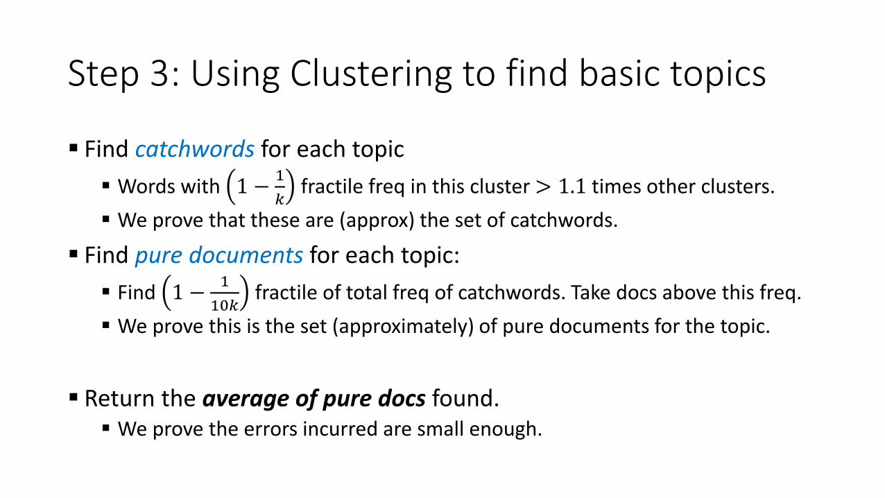
Step 3: Using Clustering to find basic topics

▪ Find catchwords for each topic

▪ Words with 1 −1

𝑘fractile freq in this cluster > 1.1 times other clusters.

▪ We prove that these are (approx) the set of catchwords.

▪ Find pure documents for each topic:

▪ Find 1 −1

10𝑘fractile of total freq of catchwords. Take docs above this freq.

▪ We prove this is the set (approximately) of pure documents for the topic.

▪ Return the average of pure docs found. ▪ We prove the errors incurred are small enough.

Step 4: Edge Topics from Basic Topics

• For each document s, find 𝒍𝟏 𝒔 and 𝒍𝟐 𝒔 , the basic topics whose catchwords have first and second highest count in s.

• 𝑋 𝑙, 𝑙′ = 𝑠 𝑙 = 𝑙1 𝑠 , 𝑙′ = 𝑙2 𝑠 , 𝑤𝑡 𝑜𝑓 𝑙′ ≥∗∗∗}

• If 𝑋 𝑙, 𝑙′ ≥∗∗, average of doc’s in 𝑋(𝑙, 𝑙′) is an edge topic.

Empirical Results : Quality

▪ Metrics▪ Topic Coherence: Log (pair-wise co-occurence) of the top 5 words in each topic.

▪ Likelihood: Given 𝑨, find MLE M and likelihood under M.

▪ Reconstruction Error: Does the topic model constructed from finite number of samples converge to a perceived ground truth.

▪ Comparison with LightLDA [Yuan, Gao, Lui, Ma (MSR), Ho, Dai, Wei, Zheng (CMU)]:

▪ Compare results on NY Times, Wikipedia and their biggest open dataset – Pubmed.▪ Compared with 100 iterations of TLC’s LightLDA.

ISLE is mostly better than LightLDA

ISLE vs LightLDA: Topic Coherence and Likelihood

For k0 = 100; 1000; 2000 basic topics and k = 10K; 20K; 50K edge topics.Edge topics were generated using 2000 basic topics.Bold is better.

Importance Sampling

Average topic coherence and log-likelihood of k0 basic topics for ISLE with r = s/10 (10%) sampling and r = s (100%).

Sampling does not significantly affect quality.

Reconstruction Error: PubMed

L1 Distance ISLE LightLDA

100K samples 0.63 Avg

1.16 Max

1.39 Avg

1.98 Max

200K samples 0.48 Avg

0.99 Max

1.31 Avg

1.90 Max

▪ Take 2 samples from corpus and compare best-matched L1 distance between the two topic matrices returned by the algorithm.

▪ This obviates knowing ``ground truth.’’ Note: we are not given generating matrix.▪ Closer is better. L1 distance range: [0, 2].

Empirical Results: Time

• 16 core workstation, dual Intel® Xeon® E5-2630 v3128 CPUs, 128GB RAM

• ISLE• VC++/VS2015, OpenMP for multi-core parallelism.• Intel® Math Kernel Library 17.x.y for parallel sparse and dense math calls.• SVD using Spectra Eigenvalue solver library, a C header reimplementation of ARPACK

with Eigen Matrix Classes and Intel MKL.• Distance calculations translated to BLAS calls, linked to MKL.

e.g. For points P and centers C (matrix columns are coordinates):

𝑳𝟐𝟐 𝑷, 𝑪 = 𝟏𝑻𝒄𝒐𝒍𝒔𝒖𝒎𝟐 𝑷 + 𝒄𝒐𝒍𝒔𝒖𝒎𝟐 𝑪 𝟏𝑻 − 𝟐𝑷𝑪

• LightLDA: MAML v3.6, 24 threads, 100 iterations

https://github.com/yixuan/spectra

http://eigen.tuxfamily.org/

PubMed Time

Computing Edge Topics from Basic Topics takes at most 2 minutes.

LightLDA in TLC 3.6 is about 2-3 times faster than in TLC 3.2 and TLC 2.8!

Time on 16 core machine

ISLE(r=s/10, 10%)

ISLE(r=s, 100%)

LightLDA (100 iter)

100 Basic topics 6 min 17 min 74 min



100000 Edge topics(from 2000 Basic Topics)

149 min 503 min 237 min

Wikipedia Time

Our running time for 100M ProductAds was 8.5 hours for 1000 topics and the coherence was -25.3

Time on 16 core machine

ISLE(r=s/10, 10%)

ISLE(r=s, 100%)

LightLDA (100 iter)




100000 Edge topics(from 2000 Basic Topics)

174 min 759 min 411 min

Potential improvements in time

• SVD solver Improvements in Spectra library

• K-means++ for initialization Explore faster seeding algorithms

• K-means, currently Lloyds Elkans, YingYang (TLC) algorithms

• Goal: Multi-node implementation, work with 1TB scale data.

Conclusion

• New topic models with large sample sets, vocabularies, and topics.

• Polynomial time algorithms with provable bounds on recovery error

• Empirical Validation: better than LightLDA in quality and time

• Scalable Implementations: more to come.

New Projects

• Flash algorithms

• Nested Dataflow

Potential Applications in Microsoft

• Bing Ads: Snippet Generation

• Office Substrate

• Triage for customer complaints.

NMF with Realistic Noise

▪ Same assumptions on 𝐵, 𝐶 (the factors) as in Topic Modeling, EXCEPT▪ We do not assume the data points are stochastically generated.

▪ Earlier provable algorithms assumed instead of Stochastic generation a strict noise model:▪ Noise 𝐴 − 𝐵𝐶 in each data point << data.

▪ Violated by most points for Topic Models!

▪ Bhattacharyya, Goyal, Kannan, Pani (ICML 2016) assume:▪ Subset Noise: For any subset of 1/10 th of the data points,

▪ Noise in average of subset in ≤ 𝜀(average of the data). Holds for many situations.

▪ Same Algorithm as for Topic Modeling works. Proof quite different (because there is no stochastic model). More efficient than previous algs.