1

Topic 4: Introduction to Exchange Rates

Part 1: Definitions and empirical regularities - The models we studied earlier include only real variables

and relative prices. We now extend these models to have a nominal side and nominal exchange rates.

- Some Basic Definitions: - nominal exchange rate (e): home currency price of a unit

of foreign currency. Note that a rise in e is a depreciation in the value of the home currency.

- real exchange rate (q): relative aggregate price levels of

two economies. Usually defined as ratio of CPIs: q=eP*/P.

2

- Purchasing power parity (PPP), hypothesis that the aggregate price level should be the same across countries when adjusted to a common currency.

*eP P Note that PPP implies that real exchange rate is constant

at value q=1.

- Relative PPP: in percent changes: % % % *e P P Currency depreciation equals inflation differential.

3

Logic of PPP - Based on the law of one price (LOP) for individual goods.

says the price of any individual good should be the same across countries when converted to same currency:

Pi = e Pi*, for individual good i

- Failure of condition implies an arbitrage opportunity to purchase good where cheap and resell where expensive:

- This should affect the prices, lowering them where they had been high, and raising them where had been low

- PPP claims this equality applies also if goods prices are

aggregated to compute CPI.

4

There are several reasons why PPP might fail to hold:

1) Different consumption baskets across countries: aggregating goods prices with different weights produces different aggregate values.

2) Nontraded goods: Nontraded goods may have different prices in different countries, because it is impossible to arbitrage these if they can’t be traded

3) trade barriers: also can prevent arbitrage

4) Imperfect competition: market segmentation lets firms set different prices for differing market conditions.

5) sticky prices, if the exchange rate changes while prices can’t adjust right away, this would cause prices of goods to be different for a while, in common units.

5

Stylized facts Transparency of statistics for the real exchange rate

- very volatile: 4x that of output.

- very persistent: serial correlation of 0.8 on average.

- The Real and nominal exchange rates move closely together. The correlation is is almost unity.

Similar characteristics to the terms of trade in Backus et al (1992).

Mussa (1986 Carnegie Rochester): also noted that the

volatility of both real and nominal exchange rates are lower during fixed nominal exchange rate regimes.

6

7

Debate over real v. nominal shocks: Nominal shocks: (Mussa position) - Using the definition of the real exchange rate above:

*Pq eP

- Then one way to explain the volatility of the real exchange rate and its comovement with e, is to assume prices are sticky:

- If money supply or demand shocks affect e, while P and

P* are fixed, then this is passed on to q. - We will study sticky price models in detail soon.

8

Real shocks: (Stockman position)

- Inverting the definition of the real exchange rate:

*

Pe qP

- Can argue that it is movements in the real exchange rate,

due to real shocks (such as productivity shocks in RBC models) that get passed on to nominal exchange rate.

- This theory also can explain the comovement of real and

nominal exchange rates.

- It can easily explain persistence of real exchange rate, since productivity shocks are usually highly persistent.

9

Questions for discussion: 1) How does the “real exchange rate puzzle” remind you of

the “relative price puzzle” we discussed previously in the context of RBC models?

2) What problems do you see with the Stockman position

(real shocks) in explaining some items on the list of stylized facts for the real exchange rate given above?

3) What shortcomings do you see in the Mussa explanation

(nominal shocks) for persistent real exchange rates, given it is based on sticky prices?

4) How might you test between the nominal shock and real

shock explanations for the real exchange rate?

10

Part 2: Time-series studies of PPP Early tests of relationship of nominal e and relative prices

(PPP) took the form of a simple OLS regression (1970s): *

tt t te p p where all variables are in logs - The test is if =1. - Most tests rejected this. - But know now that if the nominal exchange rate or

relative prices are nonstationary, we can’t use traditional confidence intervals for .

11

Unit Root tests - Next set of tests impose the assumption that =1 and

compute real exchange rate, then test if it is stationary. - The idea is that even if PPP does not hold at each point

in time, we want to test if it holds as a long-run equilibrium condition.

- The real exchange rate may be pushed away from its

equilibrium PPP value by shocks, but will it tend to return to it’s equilibrium value over time?

- So we compute: q = e x (P* / P), and apply one of a

variety of unit root tests.

12

- Early tests were not favorable to PPP: could not reject unit root in the real exchange rate.

- But literature realized this could be due to the notoriously

weak power of existing tests to reject unit root. - Frankel (1986 book chapter) showed the post Bretton

Woods data used in the preceding studies simply is not enough data to be able to reject a unit root.

Suppose the real exchange rate (q) follows an

autoregression:

ttt qqqq 1

13

And suppose the half-life is 36 months, so that the autoregressive coefficient for monthly data would be 0.981.

- The authors then demonstrate it would require 72 years

of data to be able to correctly reject unit root at 5% level. - Literature in recent years has progressively found

stronger evidence to support PPP in the long run, and the time to get there may be shorter than originally thought.

14

Approaches taken in the literature: 1) Longer Time Series: Lothian and Taylor (1996 JPE):

- 200 years of data on dollar/pd and pd/FF, strongly rejects unit root, both for full sample and pre 1945 period (since 1945-73 had fixed exchange rates).

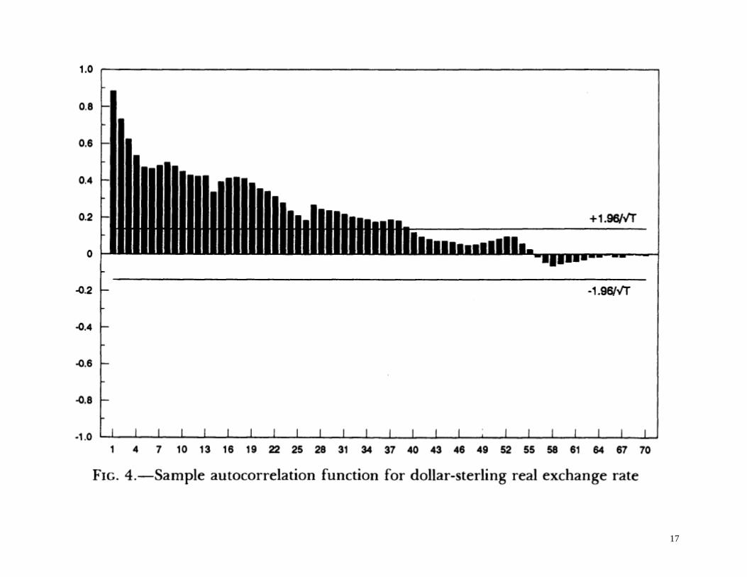
- Graphs of the autocorrelation functions show that it may

take a very long time for the real exchange rate to return to its equilibrium level, but it does eventually get there.

- Autoregressions estimate an autoregressive coefficient for the dollar pound rate of 0.887, or a decay rate of 0.113. This indicates the half life of fluctuations in the real exchange rate is log(1/2) / log(0.887) = 5.7 years.

- Similar autoregressions indicated a half-life of about 3

years for the pound/French franc real exchange rate.

15

16

17

18

19

Taylor-Taylor

20

21

2) Panel regressions: - If we need more data to get a good test, then take

multiple time series for multiple bilateral exchange rates, and use them together in a panel regression.

- Use annual data for 150 countries. They mostly reject the

unit root using critical values for panel regression. They estimate a half-life of about 4 years.

- Introduced by Frankel and Rose (JIE 1996). - Large literature using more recent panel econometric

techniques; control for contemporaneous correlation in errors (CCE).

22

Aggregation Bias: Imbs et al (QJE 2005)

- Idea: This paper questions the stylized fact that real exchange rates are persistent.

- It claims that large estimates of half-lives simply due to an econometric bias, arising from heterogeneity in the persistences of individual goods in the CPI basket.

- If econometric methods are used to control for this heterogeneity, then the estimate of the half life of PPP deviations drops to less than one year.

- Implication: There is hope for the sticky price explanation for real exchange rates, if the persistence of real exchange rates and prices both are about 1 year.

23

Imbs et. Al. Setup: For simplicity, consider a panel of just one country pair. There are N sectors indexed by i. Suppose the international relative price in each sector, itq , follows the process: 1it i i it itq q Where i represents the persistence, characterized by:

i i ,where i is mean zero.

it is the sectoral disturbance term with variance 2i and

covariance across sectors ij (reflecting common shocks).

24

Put the sectors in order of increasing persistence: 1i i Define the real exchange rate as an aggregation over sectors:

1 1

, 1N N

t j jt jj j

q q

This implies for an AR(1) specification of the real exchange rate:

1

11 1

t t t

N N

t j jt j j jtj j

q q

q

The lagged dependent variable in error term biases the least squares estimate of the persistence parameter, call it Q .

25

,lim QN Tp p

1

22

2

22

21

1 1

1 1

N

i ii

Ni ji

i iji ji i j

iN N

i jii ij

i i ji i j

where

is a weighting over the sectors.

26

The paper proves that: 1) The bias is positive if the covariance between the vector of persistence parameters i and the vector of coefficients i is positive, as this implies that the high persistence sectors have disproportionate weights in the average. 2) The positive bias tends to increase with the cross-sectoral dispersion in persistence. Note: the covariances between sectoral price residuals affect both the magnitude and sign of the bias, so we will need to control for these correlations in empirical work. The main point: in the face of heterogeneity, the persistence of the real exchange rate will not be a consistent estimate of the mean persistence of relative prices.

27

Econometric method: - Use estimation models that allow for heterogeneity -

Mean Group (MG) estimator of Pesaran and Smith (1995), a generalized fixed effects estimator that allows for heterogeneity.

- Will combine this with common correlated effects (CCE) estimator, that controls for correlation in the residuals.

Data: Eurostat, price indices for 19 two-digit consumption goods for 13 countries, monthly 1981:1-1995:12 to avoid periods with missing data. Prices relative to US dollar.

28

29

Findings

- Sectoral data appears at first to be highly persistent, as in past studies of aggregate data. Half-lives around 3 years.

- Controlling for heterogeneity and common correlated effects (MG-CCE, main case) reduces the persistence to half-life of less than one year.

- This lower degree of persistence could plausibly be explained by price stickiness.

30

Bergin, Glick, Wu (2014, JME) Idea: apply panel methods to estimate half-life of real exchange rate for fixed exchange rate period of Bretton Woods (WWII – 1973). Finding: The long half-life of aggregate real exchange rates during floating exchange rate period does not apply to the fixed exchange rate period.

31

Data:

- Bilateral nominal exchange rates with the U.S. dollar and consumer prices indices, for 20 industrialized countries.

- Source: International Financial Statistics.

- Annual in frequency 1949 to 2010. Monthly frequency starting in 1957.

32

Methodology:

- Compute real exchange rate, and estimate autoregression:

, , , ,1

( )M

j t j j m j t m j tmq c q

- Estimate for two periods: Use panel estimator that

controls for common correlated error terms, by including cross-sectional means in the regression.

- Also to control for potential bias, conduct bootstrap bias

correction procedure of Kilian (1998).

33

Results:

- Half-life of Bretton Woods period is 2.27 years; for post Bretton Woods period is 4.31 years. Confirmed in graph.

- Mussa question: why would nominal exchange rate regime affect persistence of the real exchange rate?

34

35

36

Results cont: Source of Mussa volatility finding

- Can decompose the variance of the real exchange rate.

, ,2

1var var1j t j t

j

q

- Var(q) rose by 102%, first term on right rose by 66%.

- So nearly 2/3 of rise in variance under flexible exchange rates is due to rise in persistence rather than rise in volatility of exogenous shock.

37

38

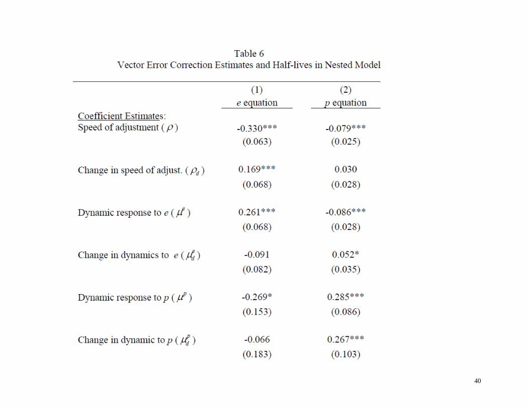
- Results cont: Why regimes matter

- Estimate a VECM with 2 equations

, , , , 1 , , 1 , , 1 ,( ) ( ) ( )e p ej t e j e j j t e j j t e j j t j te q e p

, , , , 1 , , 1 , , 1 ,( ) ( ) ( )e p pj t p j p j j t p j j t p j j t j tp q e p

- Majority of rise in real exchange rate persistence is due

to greater persistence in short run response of inflation to e shocks and p shocks: ,

ep j and ,

pp j .

- Can be interpreted as a rise in price stickiness or inertia.

- Supports use of sticky price models to explain real exchange rate behavior.

39

40

41

42

Part 3: Empirical tests of exchange rate models PPP provides a basis for a convenient starting point for a simple theory of the nominal exchange rate.

- Rearranging PPP implies that the nominal exchange should be the ratio of national price levels:

/ *e P P - This theory becomes usable if we combine PPP with a

theory of what determines the overall national price level, such as a money market equilibrium theory:

- Suppose that real money demand is a positive function of

income (y) and a negative function of interest rate (i) (we derive such conditions later in a micro-founded model:

43

,d dm m y i - And nominal money supply is exogenous: SM M - Suppose money market equilibrium condition equating

real money demand with real money supply:

,d Mm y iP

- Produces a theory of the price level: ,dP M m y i - This provides one simple theory of the exchange rate.

**

, ,*, ** *, *

d d

dd

M m y i m y iP MeM m y iP M m y i

44

**

, ,*, ** *, *

d d

dd

M m y i m y iP MeM m y iP M m y i

- A version of the “monetary approach to exchange rates” - Predicts that the home currency depreciates if the home

money supply rises, output falls, or interest rate rises (may reflect rise in expected inflation).

45

Meese - Rogoff (JIE 1983): - Study out of sample fit of exchange rate models

developed in the 1970s, such as monetary model above.

- Some early tests indicated these models fit the data fairly well, when tested “in sample.”

- Write flexible price monetary model, based on PPP, as: m and m* represent money supplies in logs, y represents

income in logs and i the nominal interest rate. The latter two terms enter because they determine the

level of real money demand in the monetary model.

* * *( ) ( )t t t t t t t

s m m y y i i

46

- The terms are parameters estimated from data. - The authors also test a sticky price version of the

monetary model, which adds an extra term involving expected future exchange rate movements.

- Begin by estimating the parameter values based on data

running from March 1973 to December 1976.

- Then generate forecast for the exchange rate for January 1977 using parameters estimated on data for preceding months, and value for the regressors for the month of the forecast. This is “out of sample forecast.”

- Then add one month of data and re-estimate the model,

and then construct the February 1977 fitted value by using actual data on right side variables for Feb. 1977.

and

1/ 77s

47

- To be concrete, for example with the flex-price model, we

would have They then calculate out-of-sample mean-squared-error - Is it a big number? Compare it to the mean-squared

change in the log of the exchange rate. That is, the m.s.e. from a “naïve” forecast of the exchange rate:

They generally found that at 1-, 3-, 6- and 12-month

horizons, the model could not “beat a random walk”.

* * *

2 / 77 2 / 77 2 / 77 2 / 77 2 / 77 2 / 77 2 / 77( ) ( )s m m y y i i

2

1

1 ( )ˆk

j jjs s

k

21

1

1 ( )k

j jj

s sk

48

49

A common interpretation of the Implications: - The result indicates that macroeconomic fundamentals

are not useful for explaining exchange rate movements. - A long subsequent literature has supported this finding,

testing various improvements on the macroeconomic model, and finding they cannot beat a random walk.

- In response, some papers use models of other types to

explain exchange rate movements. One example is to borrow from the finance literature and use models of information heterogeneity among traders.

50

Flood & Rose (EJ 1999) “Understanding Exchange Rate Volatility Without the Contrivance of Macroeconomics”.

- Note that standard macro fundamentals are not sufficiently

volatile to explain the high volatility of the exchange rate. - Build on Mussa observation: exch. rate volatility under

flexible exch rate regimes higher than under fixed regimes. - But macro fundamentals under flexible exchange rate

regimes is not noticeably higher.

- Instead argue that foreign exchange market is subject to shocks: taste shocks between home and foreign bond.

- A flexible exchange rate regime allowing international

asset trade lets these shocks affect equilibrium exch. rate.

51

Engel & West Papers (2005, 2006, 2008)

- These papers offer a reinterpretation of the earlier evidence, indicating that it need not conflict with a fundamental based model of the exchange rate.

- They borrow from asset pricing models in finance, which

posit asset price is a discounted sum of future fundamen-tals (ie stock price is discounted sum of future dividends)

where b is the discount factor x are observable fundamentals z are unobservable fundamentals

0 0(1 ) (1 )j j

t t t j t t jj j

s b b E x b b E z

52

Engel and West show: - If the fundamentals are nonstationary, then as the

discount factor approaches 1, the exchange rate implied by this model approaches a random walk.

- Intuition: Think of fundamentals as having a random walk

component, and a stationary component that fluctuates around the random walk component.

- As b goes to one, the distant future matters a lot. All the

weight goes to the permanent component of fundamen-tals because stationary component expected to die out.

53

b is discount factor, are persistence of

fundamentals 1and

54

First, is this relevant? - It depends on how big b is in practice. What matters is

the size of b and the persistence of the transitory component.

- Engel-West do some calibration and simulation

exercises. Simulate data for b=0.9, and put in standard tests, cannot reject nonstationarity of exchange rate.

- The implication is that we cannot discard models based

on fundamentals if they cannot forecast out of sample. This is what you should expect if fundamentals are highly persistent and discount factors are high.

55

One test of the theory: Granger Causality tests - If expectations for future fundamentals determine the

exchange rate, than instead of testing whether lagged fundamentals explain exchange rates, we should be testing if lagged exchange rate predicts fundamentals.

- The authors test this by Granger causality tests. - Obtain data on fundamentals from monetary model:

relative money supplies across countries, interest rate differential, inflation differential, output growth differential

- Regress fundamentals on lags of the exchange rate, and

vice versa.

- Test for significant of coefficients in regression.

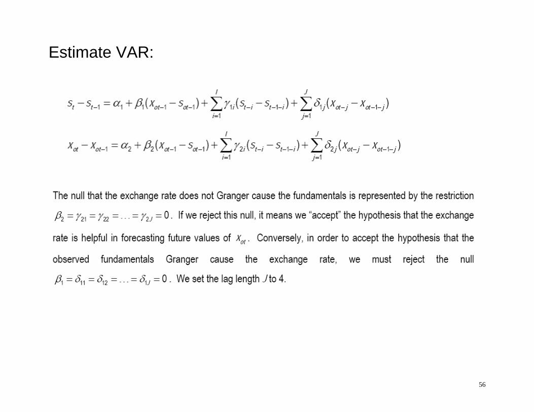
56

Estimate VAR:

57

58

Findings: - It appears that the exchange rate Granger causes

fundamentals. - But fundamentals do not Granger cause the exchange rate. - This is consistent with their theory.

59

A further test of the theory: quasi present value tests - The theory proposed above resembles the present value

model for the current account we studied earlier (CA was a discounted sum of expected changes in net output, NO.)

- Recall that to test that model, we used VARs on NO and

CA to generate a forecast of future changes in NO. These put into a present value formula to compute CA prediction.

- The authors are reluctant to fully use the present value

model here, as some of the fundamentals are assumed unobservable.

- Engel-West (2005) does part of the test, by running a VAR

on lagged fundamentals (and the exchange rate) to get a forecast of future changes in fundamentals, call it F.

60

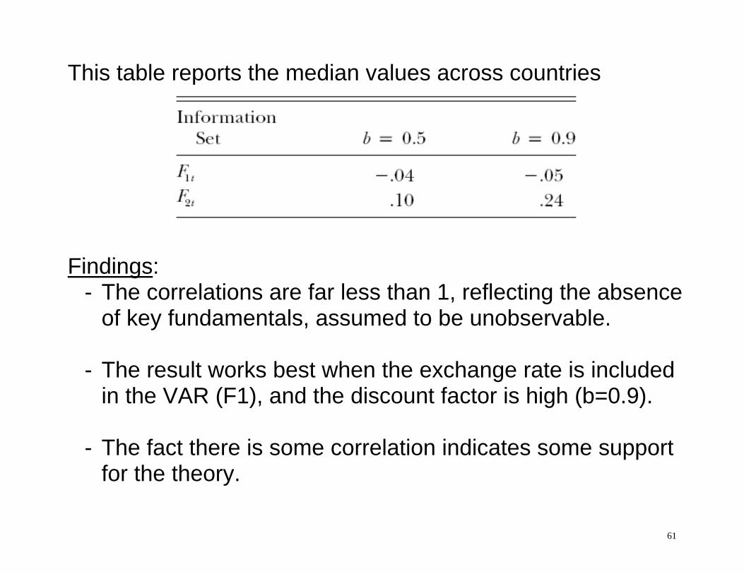
- Then just see of this F is correlated with changes in the exchange rate. Results will report correlations between measures of future fundamentals (F) and exchange rate.

- F1 is fundamentals forecast using just lagged fundamentals

in the VAR, F2 uses exchange rate also in the VAR.

61

This table reports the median values across countries

Findings: - The correlations are far less than 1, reflecting the absence

of key fundamentals, assumed to be unobservable. - The result works best when the exchange rate is included

in the VAR (F1), and the discount factor is high (b=0.9). - The fact there is some correlation indicates some support

for the theory.

62

Engel - West (2006 JMCB) goes farther in implementing the present value test, but for slightly different exch. rate model. Instead of using PPP with money demand, they start instead with monetary policy rules: interest rate reaction functions to inflation ( ) and output gap (y):

1t q t t t y ti q E y for home country * ** *

1t tq t t y ti q E y for foreign A Taylor rule: central bank raises interest rate in response to expected future inflation to try to prevent that inflation. Also raises interest rate in response to expected output above normal level, as may also be inflationary.

63

Combine these with uncovered interest rate parity condition (to be discussed later) in place of the PPP condition used in monetary model above:

*1t t t t ti i E s s

Sub in policy rules for interest rates and solve forward, to compute a forward looking equation for real exch. rate, q:

* *11

0

1 11

j

tt t t y t tj q

q E y y

Take estimates of policy parameters from Taylor rule literature and y ; q from related open-economy literature.

64

Estimate expected future inflation and output by estimating a VAR on these variables, and generating forecast. Substitute forecasts and parameters into the present value condition above (as we did previously in class for present value tests of current account models). Engel-West (2006) used data on US dollar-Deutsch Mark exchange rate, 1979:10-1998:12.

65

66

Results limited because expectations of market participants depend on many things other than just the lagged values. - Figure not terrible. Correlation between model prediction

and data on real exchange rate is 0.32.

- But prediction is much less volatile; sdev is 1/5 of data.

67

Engel-Mark-West (2008): in addition to replicating the results from earlier papers, it conducts several additional tests Volatility: It critiques the claim (ie from Flood-Rose) that fundamentals can’t explain the exchange rate, because the volatility of exchange rates is much higher than of macro fundamentals. Makes the point that is the pdv of future fundamentals that matters, and if they are nearly nonstationary with low discounting, then the pdv might be quite volatile. Define:

68

Estimate expectations from forecast based on 4th order autoregression. Table reports variance of first difference in each monetary fundamental (h) to that of exchange rate (s), under alternative assumptions about discount factor. Table shows that monetary fundamentals can generally account for a fair fraction of exchange rate variance (around 0.5 on average).

69

70

Survey Measures of Expectations: An alternative to VARs as method to proxy for expectations of future fundamentals is to use survey data. Consensus Forecasts surveys economic forecasters twice a year on expectations for the current year, next five and next 6-10 years of these variables. Estimate the pdv equation from above in first differences,

Data: April 1997 – Dec 2006. Because data series short, pool countries and estimate as a panel over US real exchange rate with 11 countries.

71

Note that the coefficient on inflation is negative, contrary to the monetary model. The reason is the monetary policy rule. Question: can you explain why this is the case?

72

Questions for Discussion: 1) We see the important role of expectations. What do you

think about the merits of the alternative ways of dealing with expectations here: VARs, surveys? Any better ideas?

2) Are there more general monetary models you think might

work better (Several have been tried in the literature)