top-of-the-line corrosion control by continuous chemical
TRANSCRIPT

Department of Chemistry
Top-of-the-Line Corrosion Control by
Continuous Chemical Treatment
Mike C. Oehler
This thesis is presented for the Degree of
Doctor of Philosophy
of
Curtin University
December 2012

I
Declaration
To the best of my knowledge and belief this thesis contains no material
previously published by any other person except where due acknowledgment
has been made.
This thesis contains no material which has been accepted for the award of
any other degree or diploma in any university.
Signature: ………………………………………….
Date: ………………………...
II
Summary
Top-of-the-Line (TOL) corrosion is a severe problem associated with the
transportation of wet natural gas. It has the potential to cost the oil and gas
industry millions of dollars every year through lost production and the
necessity to replace effected pipelines.
Research was carried out in order to better understand and estimate the TOL
corrosion risk and its control. The first part of the research focused on the
development of a domain diagram. The TOL corrosion domain diagram was
designed to gain a better understanding of how carbon dioxide partial
pressure, acetic acid concentration, and temperature influence TOL
corrosion at a constant condensation rate. It summarises the effects of some
important parameters on TOL corrosion. TOL corrosion tests were
performed with three different carbon dioxide partial pressures of 5 bar
(72.5 psi), 10 bar (145 psi), and 20 bar (290 psi), and different acetic acid
concentrations of 0 ppm, 500 ppm, and 1000 ppm. The sample temperature
was also varied at 30 ⁰C and 80 ⁰C. The gas temperatures were adjusted to
91 ⁰C and 115 ⁰C to maintain a constant condensation rate in both
temperature regimes of 0.40 g/m2/s.
The next part of the research was focused on volatile corrosion inhibitors
(VCIs). 16 potential VCI compounds (Aminoethylpiperazine, Amino-
morpholine, Aniline, Benzylamine, Cyclohexylamine, Dicyclohexylamine,
Diethylamine, Dimethylethylamine, Methyldiethanolamine, Methyl-
morpholine, Methylpiperazine, Morpholine, Octylamine, Picoline,
Pyridazine, and Pyridine) were chosen and tested in a variety of TOL
corrosion test rigs. It was possible to identify the properties and
characteristics of a potential VCI compound in the presence of acetic acid.
The same VCIs were also tested in a rotating cylinder electrode test set-up
using electrochemistry, mainly linear polarisation resistance (LPR) and
electrochemical impedance spectroscopy (EIS), to test their Bottom-of-the-
Line (BOL) inhibition ability as well as their mechanism of inhibition. All of
the compounds showed BOL inhibition capability. One compound stood out

III
as a good film former on carbon steel despite an uncommon molecular
structure for a film forming corrosion inhibitor.
Design modifications for the different TOL corrosion set-ups used in the
experiments were devised using the data and experience gained in this
research. A modified TOL corrosion apparatus was constructed, capable of
high pressure, high temperature TOL corrosion testing, with the potential to
standardize TOL corrosion and VCI testing was suggested.

IV
Publications, Presentations, Posters
Oehler, M.C., Bailey, S.I., Gubner, R., (2013). Top-of-the-Line Corrosion
Research under High Pressure. Accepted Paper at NACE Corsym 2013,
Chennai, India.
Oehler, M.C., Bailey, S.I., Gubner, R., Gough, M. (2012). Testing of Generic
Volatile Inhibitor Compounds in Different Top-of-the-Line Laboratory Test
Methods. Paper # C2012-0001483. Paper presented at NACE Corrosion
2012, Salt Lake City, USA.
Oehler, M.C., Bailey, S.I., Gubner, R., Heidersbach, K., Gough, M. (2012).
Comparison of Top-of-the-Line Corrosion Test Methods for Generic Volatile
Corrosion Inhibitor Compounds. Oral Presentation at NACE - 3rd
International Top-of-the-Line Corrosion Conference, Bangkok, Thailand.
Oehler, M.C., Comparison of Different Top-of-the-Line Corrosion
Laboratory Test Methods (2011). Poster presentation at NACE Corrosion
2011, Houston, USA.

V
Acknowledgements
I sincerely acknowledge my main supervisor, Dr. Stuart Bailey, for his
contribution, discussions, guidance, and support during the course of the
project. I would also like to recognise Dr. Brian Kinsella, Dr. Doug John, and
Dr. Thomas Ladwein for giving me the opportunity to start my PhD by
research at Curtin University in Perth. I would also like to thank Dr. Rolf
Gubner, director of the Corrosion Centre at Curtin University, for providing
me with a top class corrosion laboratory and equipment. He was also
building bridges for me, which opened up opportunities to meet people in
the field of materials and corrosion.
I would also like to acknowledge the contribution from Chevron Energy
Technology Company, Nalco Pacific Pte Ltd, and the Curtin International
Postgraduate Research Scholarship for their financial contribution, for
without it, the work would not have been possible. Special thanks goes to
Krista Heidersbach (Chevron ETC), Dallas Thill (Chevron ETC), and Mark
Gough (BP – formerly Nalco) for their expertise, guidance, and vivid
discussions throughout the course of the project. I am sincerely grateful.
The Australian and Western Australian Governments and the North West
Joint Venture Partners as well as the Western Australian Energy Research
Alliance (WA:ERA) are acknowledged.
A special thank you also goes to the laboratory staff from Nalco Singapore,
especially Si Lin and Nadiah, for helping me out with my experiments and
making my stay in Singapore an exceptional experience. I also want to
mention the staff of the chemistry department (especially Tanya Chambers,
Peter Chapman, and Thomas Becker) and the corrosion centre (Lomas
Capelli) who were very supportive during the course of my PhD, everyone in
his or her own way. My fellow research students in the Corrosion Centre
students (especially Laura, Priya, and Amalia) and Chemistry Department
(Karen and Elaine) deserve also a special mention for making the experience
one to remember.

VI
I also want to thank Jens Maier and Anja Werner for introducing me into a
new world at Curtin University and Perth, making my move to Australia an
easy one.
Special appreciations go to my girlfriend, Gizelle Cuevas, for the support and
patience with me during the research and write-up of this thesis. I’m sure it
wasn’t always easy. Thank you for brightening up every day of my life!
Lastly, I want to give the deepest gratitude to my family, to my loving mother
Gabi, my brother Marco, and in memory of my father, Helmut. Thank you for
always believing and supporting me.
VII
List of Abbreviations
A Area
AAS Atomic absorption spectrometry
A-HCT Altered Horizontal Cooled Tube
(aq) Aqueous
B Stern-Geary constant
ba Beta A value (0.12)
bc Beta C value (0.12)
BOL Bottom-of-the-Line CFP Cooled Finger Probe
CR Corrosion rate
DEA Diethylamine
DMEA Dimethylethylamine
EDX Energy dispersive X-ray
EW Equivalent weight
(g) Gaseous
IC Iron concentration
icor Corrosion current density
IE Inhibition efficiency
IFM Infinite focus microscope
I-HCT Improved Horizontal Cooled Tube
HCT Horizontal Cooled Tube
Icor Corrosion current density
K1 Constant (3.27 *10-3 mm
g/A cm yr)
LPR Linear polarisation resistance
m Mass
MDEA Methyldiethanolamine
N Number of Specimens
NP Number of pitted specimens
OCP Open circuit potential
P Pitting probability
pCO2 Partial pressure of CO2
PD Potentiodynamic
PIG Pipeline inspection gauge
Ra Arithmetical mean roughness
RCT Charge transfer resistance
RP Polarisation resistance
RS Solution resistance
RCE Rotating cylinder electrode
Rz Ten-point mean roughness
SEM Scanning electron microscope
t Time
TA Temperature Autoclave
TS Temperature Sample
TOL Top-of-the-Line
VCI Volatile corrosion inhibitor
WCO World Corrosion Organisation
WL Weight loss
Units
A Ampere
cm3 Cubic centimetre
⁰C Degree Celsius
g Gram
h Hours
Hz Herz (Frequency)
m2 Square metre
mL Millilitre
mm Millimetre
m Micrometre
mV Millivolts
ppm Parts per million
rpm Revolutions per minute
s Second
V Volt
y Year

VIII
Table of Contents
Declaration ........................................................................................................ I
Summary .......................................................................................................... II
Publications, Presentations, Posters ............................................................... IV
Acknowledgements .......................................................................................... V
List of Abbreviations ......................................................................................VII
Table of Contents ......................................................................................... VIII
1. Introduction ............................................................................................... 1
1.1. Top-of-the-Line Corrosion .................................................................. 1
1.2. Top-of-the-Line Corrosion Control ..................................................... 2
1.3. Research Objectives ............................................................................. 4
2. Top-of-the-Line Domain Diagram ............................................................ 5
2.1. Introduction ......................................................................................... 5
2.1.1. CO2 Corrosion ............................................................................... 5
2.1.2. Effect of Acetic Acid on CO2 Corrosion ........................................ 7
2.1.3. Top-of-the-Line (TOL) Corrosion ................................................ 8
2.2. Experimental ..................................................................................... 12
2.2.1. Pressure Reactor and Corrosion Sample .................................... 12
2.2.2. Preparation of a TOL Corrosion Test ......................................... 14
2.2.3. Corrosion Rate Determination ................................................... 15
2.2.4. Condensation Rate Determination ............................................. 19
2.2.5. Test Conditions ........................................................................... 20
2.2.6. Corrosion Sample Identification ................................................ 21
2.2.7. Surface Investigation .................................................................. 22
2.3. Results and Discussion ...................................................................... 23
2.3.1. Horizontal Cooled Tube Test development ................................ 23
2.3.2. Top-of-the-Line Corrosion Domain Diagram ............................ 24
2.4. Conclusions ........................................................................................ 41

IX
3. Generic Volatile Corrosion Inhibitor Compound Investigation ............. 42
3.1. Introduction ....................................................................................... 42
3.1.1. CO2 Corrosion Inhibition ............................................................ 42
3.1.2. Top-of-the-Line Corrosion Inhibition ........................................ 43
3.2. Experimental ..................................................................................... 46
3.2.1. Generic Volatile Corrosion Inhibitor Candidates ...................... 46
3.2.2. Horizontal Cooled Tube (HCT) Test .......................................... 48
3.2.3. Cooled Finger Probe (CFP) Test ................................................. 50
3.2.4. Altered Horizontal Cooled Tube (A-HCT) Test .......................... 54
3.2.5. Rotating Cylinder Electrode (RCE) Test .................................... 56
3.2.6. Corrosion Rate ............................................................................60
3.2.7. Inhibition Efficiency ................................................................... 61
3.3. Results and Discussion ...................................................................... 62
3.3.1. Blank Test – No Inhibitor ........................................................... 62
3.3.2. Low performing VCIs - Results .................................................. 71
3.3.3. High Performing VCIs - Results ................................................. 98
3.3.4. Conclusion Generic VCI Compounds ....................................... 129
4. Top-of-the-Line Corrosion Test Set-ups ................................................ 131
4.1. Introduction ...................................................................................... 131
4.2. Discussion ........................................................................................ 132
4.2.1. Horizontal Cooled Tube (HCT) Test ........................................ 132
4.2.2. Altered Horizontal Cooled Tube (A-HCT) Test ........................ 134
4.2.3. Cooled Finger Probe (CFP) Test ............................................... 135
4.2.4. Rotating Cylinder Electrode (RCE) Test .................................. 136
4.3. Conclusion Improved TOL Corrosion Research Test Method ....... 138
5. Conclusions and Future Work ............................................................... 140
5.1. Conclusions ...................................................................................... 140
5.2. Future Work .................................................................................... 142
6. Bibliography ........................................................................................... 145
1
1. Introduction
Corrosion is an often overlooked, but omnipresent phenomenon. It was
estimated by the World Corrosion Organisation (WCO) in 2010 that 3% of
the world’s GDP, $ 2.2 trillion was the annual direct cost of corrosion
worldwide (Hays 2010). This huge number makes the annual corrosion costs
in the US oil and gas industry in exploration, production, refining, and
pipelines of about $ 12 billion look comparatively small. (Koch et al. 2002).
Corrosion in the oil and gas industry is still taken very seriously since
millions of dollars can be saved using the right treatments or making the
right choices. An even bigger factor is that corrosion is also associated with
numerous fatalities, injuries and environmental tragedies all over the world
(NTSB 1969- 2012) (Bills and Agostini 2009).
To keep incidents to the bare minimum, research is undertaken in many
directions; one of which is CO2 corrosion and its mitigation. CO2 corrosion,
also known as “sweet corrosion” is the prevalent form of internal corrosion
for carbon steel pipelines. Carbon steel is the most common pipeline
material, despite the fact that it is prone to CO2 corrosion. Nevertheless, with
the right corrosion prevention programs, like inhibition or pH stabilisation,
along with corrosion monitoring programs, it is a more cost effective solution
than higher alloyed steels.
1.1. Top-of-the-Line Corrosion
“Vapour-phase corrosion due to the condensation of water vapour in the
presence of acid gases and in the absence of hydrocarbon condensate has
been identified as the corrosion mechanism in the Crossfield gas gathering
system”. This was concluded in the investigation of a pipe burst in the
Crossfield gas gathering system near Calgary, Alberta, Canada in 1985 (Bich
and Szklarz 1988). This was most likely one of the first descriptions Top-of-
the-Line corrosion induced failure in a CO2 dominated environment.

2
TOL corrosion can occur when hot wet natural gas is transported in a poorly
insulated pipeline with a high heat transfer coefficient to the surrounding
area; for example subsea pipelines. The gas is cooled down rapidly and the
water vapour condenses at the pipe walls. The condensed water is very
aggressive and often referred to as “hungry water” due to the lack of
buffering agents and dissolved iron. The CO2 dissolves in the water and is
converted into carbonic acid, lowering the pH, causing the water to become
more aggressive. It is reported that a condensation rate of 0.25 g/m2/s is
sufficient to induce TOL corrosion in these conditions (Gunaltun and Larrey
2000). The necessary condensation rate is lowered by a magnitude as soon
as a sufficient amount of organic acids are present.
Organic acids, predominantly acetic acid, are a very common by-product in
the natural gas production. Concentrations of about a few hundred to a few
thousand ppm are not uncommon, and they are reported to increase the
corrosion rate and affect the protective scale formation even in relative low
concentrations.
1.2. Top-of-the-Line Corrosion Control
Many efforts to mitigate TOL corrosion have been suggested and tested.
Some of these efforts are more successful and practical than others. As long
as a field is in the building stage, the first kilometres can be built of corrosion
resistant alloys without heat insulation. Water vapour then can be condensed
out so it is no longer present further down the line. Another solution is
burying the pipeline deeper into the ocean floor, increasing the heat
insulation. These are engineering efforts that can be implemented in newly
developed fields but not in already developed and working pipelines. In these
cases, inhibition plays a major role in TOL corrosion mitigation.
Major hurdles are the distribution of the inhibitor to the TOL. One of the
more common techniques is inhibitor batch treatment. A sticky long chain
organic inhibitor is put in between two Pipeline Inspection Gauges (PIGs)
and it is run through the pipelines. Unfortunately, the production of the pipe

3
or even large parts of a field needs to be shut down for this procedure,
resulting in a big loss for the operating companies.
Another method would be a rather novel approach using a spray PIG. The
PIG uses the Venturi Effect and sprays solution from the Bottom-of-the-Line
(BOL) with a high inhibitor concentration to the TOL. The field doesn’t need
to be shut down completely, but the pipeline still needs a launching and
receiving point for PIGs as well as the risk of a PIG being stuck in a pipeline.
Another promising approach is Volatile Corrosion Inhibitors (VCI). VCIs are
commonly known to be small chain amines due to the required volatility.
These VCIs are continuously injected into the BOL, utilizing the same
injectors installed for conventional BOL corrosion inhibitors. It is not well
understood how VCIs work, but commonly, VCIs are thought to evaporate
and co-condense at the TOL with all the other fluids and inhibit the CO2
corrosion directly where it occurs. Nevertheless, most of the commercially
available VCIs are not yet effective enough at inhibiting the TOL corrosion
for them to be used as the sole countermeasure. So far, they are mainly used
in combination with PIGs to extend the cycles in which they have to be used,
which is already an enormous benefit.
This research investigates several generic potential VCI compounds; some of
them are in use in commercial formulations. As mentioned above, it is not
yet clearly known how they reach the TOL (foaming, volatility) and by which
mechanism they inhibit (neutralizing, film forming) TOL corrosion.
Different laboratory-based equipment was used to gain a better
understanding of TOL corrosion under different conditions and investigate
the performance and inhibition mechanism of the different VCIs.

4
1.3. Research Objectives
Developing a TOL corrosion domain diagram with variable carbon
dioxide partial pressure, acetic acid concentration, and temperature
under constant condensation rate
Gain a better understanding of TOL corrosion testing under high
carbon dioxide partial pressures
Find a working VCI compound able to be used in a formulated
commercial VCI
Examine the mechanism of TOL corrosion inhibition through various
VCI compounds
Identify properties of a potential generic VCI compound
Improve the existing TOL corrosion test methods
Develop a TOL corrosion test method with the potential to be
accepted as standard test method for VCI evaluation

5
2. Top-of-the-Line Domain Diagram
2.1. Introduction
2.1.1. CO2 Corrosion
CO2 corrosion in the oil and gas industry was discovered for the first time in
the 1940s and has been a problem in the industry ever since. Several
research teams all over the world keep investigating the phenomenon to gain
a better understanding of the mechanisms of CO2 corrosion (Crolet and
Bonis 1983; Sun and Nesic 2006; Tan et al. 2010). Nevertheless, the exact
mechanism is still widely debated. The following equations display the trail
of CO2 becoming a corrosive environment for carbon steel in combination
with water.
CO2 in the gas phase and in the liquid phase are in equilibrium.
Equation 1
CO2 then dissolves in the water phase forming carbonic acid.
Equation 2
H2CO3(aq) dissociates in two steps releasing two H+ as seen in the next
equations.
Equation 3
Equation 4
The amount of carbonic acid and all subsequent carbonates is highly
dependent on the CO2 partial pressure (Equation 1- Equation 4) which in
turn has a direct influence on the corrosivity of the liquid phase.

6
The exact mechanism how CO2 corrodes carbon steel is still under debate
and is very much dependent on other factors like water chemistry,
temperature, pH, partial pressure and others. The overall equation for CO2
corrosion of carbon steel is also often shown as
Equation 5
Dugstad concludes in his review paper that CO2 is assumed to contribute to
the cathodic reaction rate in two different ways. H2CO3 can be directly
reduced and the dissociation of H2CO3 can serve as a source of H+ ions
(Dugstad 2006). The equation for direct reduction would look like the
following.
Equation 6
The free iron (II) ion then can react with the carbonate ion to form iron
carbonate.
Equation 7
The iron carbonate then accumulates in the water phase. With ongoing
corrosion, the concentration of iron carbonate in solution will increase until
it hits the saturation limit and an iron carbonate film starts forming on the
carbon steel surface. The precipitation rate is a function of supersaturation
and temperature (Sun and Nesic 2006). It was shown that FeCO3 is more
soluble at lower temperatures and therefore higher FeCO3 concentrations are
necessary to reach supersaturation at lower temperatures (Johnson 1991;
Dugstad 1998). Once an iron carbonate film has formed it stays protective
even at a much lower supersaturation (Dugstad 1998). The iron carbonate
then acts as a protective corrosion product layer retarding further corrosion.
Once again, the protectiveness of the corrosion layer depends, strongly on
environmental parameters like surface condition, temperature, pH and
others (Nesic et al. 2001; Nesic et al. 2002).

7
2.1.2. Effect of Acetic Acid on CO2 Corrosion
Acetic acid is a weak organic acid that provides a single hydrogen ion upon
dissociation. The connection between organic acids and CO2 corrosion was
reported for the first time as early as 1944 by Menaul in the Oil and Gas
Journal (Menaul 1944). Later it has been shown that mainly formic, acetic,
propionic and, butyric acid are present with acetic acid being by far the most
prevalent at up to 90% (Dougherty 2004). Studies have shown that there is
very little difference in the corrosion behaviour of the diverse low molecular
weight organic acids (Fajardo et al. 2007). Therefore, the focus here will be
on the most abundant, acetic acid, and its contribution to CO2 corrosion.
Over the years many different even contradictory theories were put forward
to explain the contribution of acetic acid to CO2 corrosion. In 1999 it was
published that acetate (CH3COO-), which is dissociated acetic acid, increases
the corrosion rate (Hedges and Mc Veigh 1999). At the same conference it
was concluded that it is in fact not the acetate but just the concentration of
free acetic acid that increases the corrosion rate (Crolet et al. 1999). Many
experiments and publications later, it can be concluded that the latter theory
is the right one (George and Nesic 2007).
Acetic acid is reported to increase the cathodic corrosion reaction of bare
steel in two ways. It is believed that acetic acid supplies H+ ions to the
corrosion site (by dissociation) very similar to CO2 corrosion. Additionally, it
is directly reduced on the steel surface (Garsany et al. 2002; Crolet and Bonis
2005) in form of Equation 8.
Equation 8
In real life applications, iron carbonate scale is often present on the metal.
The effect of acetic acid on the growth, protectiveness and thickness of an
iron carbonate layer is also the subject of contradicting publications. In 1999,
it was published that acetic acid reduced the thickness and protectiveness of
the corrosion layer (Hedges and Mc Veigh 1999). Some more recent
publications state that there is no significant effect on the iron carbonate
scale formation and its protectiveness (Nafday and Nesic 2005).

8
Another approach to explain the contribution of acetic acid in relation to
corrosion product layers was made by Fajardo et al. by arguing that acetic
acid initiates a “scale undermining effect”. Thicker iron carbonate scales in
presence of organic acids were found. It was concluded that plenty of iron
carbonate was formed but due to the higher corrosion rates initiated by
acetic acid, it took longer for the film to take a foothold retarding further
corrosion. (Fajardo et al. 2007).
Acetic acid also seems to induce localized corrosion in different
environments. It was reported that acetic acid induces a local potential
difference promoting the initiation of localized corrosion (Amri et al. 2009).
A higher concentration was also connected to an increased pit penetration
rate (Gulbrandsen and Bilkova 2006). Acetic acid has also be found to
exhibit corrosion inhibitive effects on the anodic part (Gulbrandsen and
Bilkova 2006), but it still increases the overall corrosion rate.
Crolet et al. showed also that it is possible, at least in low CO2 partial
pressures, that genuine acetic acid corrosion can occur and replace iron
carbonate with iron acetate. Iron acetate has a much greater solubility
decreasing the protectiveness of the scale drastically (Crolet et al. 1999).
It has also been reported that acetic acid strongly contributes to, or even is
necessary for Top-of-the-Line corrosion (Dougherty 2004).
2.1.3. Top-of-the-Line (TOL) Corrosion
Many TOL corrosion problems have been reported, especially in the Asia-
Pacific region (Gunaltun et al. 1999; Gunaltun 2006; Gunaltun et al. 2010).
TOL corrosion has been cited as one of the most complex forms of corrosion
in the oil and gas industry (Bailey 2010). It is a specific form of CO2 corrosion
limited to the production and transportation of wet gas in carbon steel
pipelines with a stratified flow regime (Figure 1).
TOL corrosion was reported for the first time in 1981 by Paillassa et al. in a
H2S containing gas field in France (Paillassa et al. 1981). It didn’t take too
long before the first case was described in a CO2 corrosion dominated gas
9
field (Bich and Szklarz 1988). Studies have been conducted and awareness
has been raised ever since, but TOL corrosion is still not yet fully understood.
Figure 1: Schematic cross-section of a gas pipeline
A key factor to consider in trying understanding TOL corrosion is the pipe
and gas temperature. The most incidences of TOL corrosion are in the first
kilometres of carbon steel pipelines where the gas is still comparatively hot
and moist and the pipe is cold. These conditions are found in poorly
insulated subsea pipelines, river crossings or upheaval buckling sections.
This combination results in a high rate of condensation. Reportedly the
condensation rate needs to be above 0.15-0.25 g/m2/s to initiate TOL
corrosion in a low organic acid environment (Gunaltun and Belghazi 2001).
It also has been reported that the condensation rate can be even as low as
0.025g/m2/s with very high (2500 ppm) concentrations of organic acids
(Gunaltun et al. 2006) making TOL corrosion possible even in rather well
insulated pipelines.
The condensing water is often referred to as “hungry water” because no
buffer and low pH values are present. Co-condensing organic acids and
dissolved CO2 decrease the pH of the condensate even further making it even
more aggressive. A race between iron carbonate saturation (and therefore

10
iron carbonate precipitation) and dilution by further condensation
commences when water first condenses. The carbon steel pipeline corrodes,
saturating the condensed water with iron carbonate. The constant supply of
condensing liquid keeps diluting the solution. Eventually a droplet will form
and either rinse down the side wall or drop off the TOL. In the case of a low
condensation rate, the pH will increase and a protective corrosion product
layer can form, mitigating further corrosion (Andersen et al. 2007). At high
condensation rates this is not the case and corrosion keeps going, rather
unrestricted.
Temperature also plays a major role in the formation of corrosion products.
As for general CO2 corrosion, the protectiveness of a FeCO3 layer depends on
the temperature of the substrate on which it is grown. As described in section
2.1.1, a protective FeCO3 layer is more likely to form at elevated temperatures
due to the supersaturation levels required.
The concentration of acetic acid at the TOL is driven by the liquid/ vapour
equilibrium of free acetic acid at the Bottom-of-the-Line (BOL) and total
acetic acid at the TOL. The distribution of free acetic acid at the TOL depends
then mainly on the pH of the condensed liquid (Hinkson et al. 2010). The
percentage of free acetic acid at the TOL or the BOL can be calculated by the
following formula:
Equation 9
with % CH3COOH is the percentage of undissociated acetic acid, pH of the
solution, and pKa of the acid, in this case acetic acid. It is possible to
calculate the percentage of undissociated acetic acid for the necessary pH
range and plot it in a graph (Figure 2). It can be seen that the dissociation of
acetic acid is highly dependent on the pH of the solution.
Besides the temperature, condensation rate and acetic acid concentration the
gas velocity also plays a role in TOL corrosion. At low velocities, stagnant
droplets are formed whereas at higher gas velocities the droplets are sliding
along the TOL and eventually slide to the BOL. For stagnant droplets it is

11
easier to form a protective FeCO3 layer whereas sliding droplets are generally
not in contact long enough with the steel and rather form a non-protective
layer (Singer et al. 2009). In many of the case studies localized corrosion was
reported at the TOL. There seems to be a strong correlation between
localized attack and acetic acid and temperature (Singer et al. 2009).
Many different laboratory test setups have been developed to investigate
TOL corrosion. Large flow loops are used to replicate field conditions as
closely as possible under laboratory conditions (Nyborg et al. 2009; Singer et
al. 2010) but they are a large, labour intensive piece of equipment and
expensive to maintain and run. Then there are many test setups replicating
TOL corrosion in bench top experiments for easier handling and greater
flexibility (Pots and Hendriksen 2000; John et al. 2009; Chen et al. 2011).
Many TOL corrosion experiments are even conducted with a specimen
submerged in a glass cell, similar to BOL corrosion tests (Amri et al. 2011). It
is difficult to implement all factors into a single test rig and therefore
priorities and research objectives have to be defined.
Figure 2: Acetic acid dissociation curve
0
10
20
30
40
50
60
70
80
90
100
2 3 4 5 6 7 8
% o
f C
H3
CO
OH
pH of solution

12
2.2. Experimental
2.2.1. Pressure Reactor and Corrosion Sample
The test reactor is a slightly modified version of a commercially available 316
stainless steel 2 L PARR high pressure reactor. It is built to withstand up to
130 bar pressure at 350° C. It is equipped with an internal purge tube and a
gas outlet, both sealed with a high pressure valve. It is also fitted with a
rupture disc that releases the internal pressure in case it exceeds its
maximum limit. Two independent pressure gauges are fitted as well; an
analogue gauge and a digital gauge which is connected to a PARR control
unit. The control unit is connected to a thermocouple to measure
temperature, a pressure gage to read pressure inside the reactor, and a
furnace to control the temperature. An upper and lower safety limit for both
the temperature and the pressure can be set, where the control unit cuts off
the power and the reactor cools down to prevent the pressure or temperature
from rising further.
The reactor in its original state as supplied by the manufacturer is equipped
with an internal cooling coil through which water is pumped. This cooling
coil was removed and the TOL corrosion set up was installed instead. A
13 cm long ¼ inch carbon steel tube (ASTM-A179 2005), bent into a
rectangular U-shape using a tube bender, was attached as corrosion sample
using stainless steel Swagelok fittings, Swagelok elbows, and Teflon ferrule
tube fittings.
After the tube was bent into shape, a heat treatment was conducted. The
sample was placed inside a furnace for 90 minutes at 650 °C to remove
residual stresses in the material (ASM 1998) induced by the bending process.
An inhibited cooling fluid (5% sodium nitrite in water) was pumped through
the test sample at a controlled temperature to initiate a temperature
difference but prevent internal corrosion (Hayyan et al. 2012). Due to the
lower temperature of the carbon steel pipe, condensation occurred on the

13
outside of the pipe, triggering condensed water corrosion as an analogue of
TOL corrosion.
1 cm of each side of the carbon steel tube was inside the fittings; therefore, 11
cm of the tube can be considered as the sample length, producing a total
surface area of 22.14 cm2. The chemical composition of the sample (as
provided by the manufacturer) is listed in Table 1 below.
Table 1: Chemical analysis of the tube material used as corrosion samples
[%] C Mn P S
Test samples 0.079 0.429 0.014 0.007
ASTM A179 0.06- 0.18 0.27- 0.63 <0.035 <0.035
Figure 3: Schematic and image of the Horizontal Cooled Tube test set-up

14
2.2.2. Preparation of a TOL Corrosion Test
The test solution (650 mL of milliQ water) was pre-purged with high purity
CO2 (99.99% pure) for at least two hours inside the body of the pressure
reactor. In the meantime, the carbon steel tube (already bend and heat
treated) was internally and externally sandblasted in a Hafco Sandblasting
cabinet to ensure a smooth and clean surface. Throughout the duration of the
research, the same sandblasting garnet product was used; old and abraded
garnet was constantly filtered out of the sandblaster cabinet and the garnet
was periodically topped up wish fresh product to ensure a reproducible
surface finish. After the sample was sandblasted it was put upside down into
a beaker of acetone and treated for 5-10 minutes in an ultrasonic bath to
thoroughly clean the specimen inside and out. The cleaned sample was then
rinsed with milliQ water and acetone and subsequently dried in an oven for
20 minutes at 70 ⁰C. After the 20 minutes it was left in a vacuum desiccator
to cool down to room temperature to be weighed.
After the sample was weighed, it was attached to the head of the reactor
using the Teflon and stainless steel tube connections. The appropriate
amount of acetic acid was added to the solution. The head of the pressure
reactor was then attached to the body and tightened using the split ring and
drop band according to the specifications provided by PARR. To remove any
residual oxygen in the system, the closed up pressure reactor was allowed to
purge for another 10 minutes with CO2 through the purge tube.
After the 10 minutes of pre-purging, the reactor was pressurised to 20 bar
and subsequently depressurised using the same high purity CO2. This
pressurizing – depressurizing cycle was repeated four times to reduce the
oxygen to a minimum. During the fifth pressurisation the system was
allowed to equilibrate for 20 minutes at 20 bar.
After the 20 minutes, the reactor was sealed and placed into a controlled
heating sleeve and heated to the appropriate temperature of the test (91°C or
115 °C). After the temperature was reached, cooling of the tube was started
and the test was considered to be initialized.

15
The procedure for low pCO2 testing was the same as above up to the
pressurizing and depressurizing cycles. After the fourth cycle to 20 bar, the
pressure was reduced to 5 or 10 bar (depending on the test) and held for
20 minutes to equilibrate. Afterwards, the pressure was topped up to 20 bar
with nitrogen and again held for 20 minutes.
The residual oxygen was measured using an Orbisphere for some tests to
verify whether or not the method described above is achieves the intent of an
oxygen free environment. The oxygen concentration was verified to be below
4 ppb in all tested cases.
2.2.3. Corrosion Rate Determination
The corrosion rate was determined in two ways, by weight loss and by
analysing the iron concentration in the bulk solution. Clarke’s solution was
used to determine the weight loss of the samples. The solution was prepared
in batches and used for several specimens.
2.2.3.1. Clarke’s Solution
Every batch of Clarke’s solution was prepares using the chemicals as stated
in the standard ASTM-G1. The sequence of preparation was as the following:
A 1 L volumetric flask was filled half with hydrochloric acid (HCl)
(ASTM-G1 2003) (ASTM-G1 2003) (ASTM-G1 2003) (ASTM-G1
2003)
50 g of stannous oxide and 20 g of antimony trioxide was weight on an
analytical balance and dissolved in the HCl
The volumetric flask was filled up with HCl to exactly 1 L
A stirrer bar was placed into the volumetric flask which was
subsequently covered and stirring was conducted for 24 hours
After 24 hours, the solution was filtered using a vacuum filter unit and
filter paper sheets
The last step might be repeated in case the solution was not clear

16
The filtered Clarke’s solution is ready to use and can be stored in a
sealable glass bottle
2.2.3.2. Corrosion Rate by Weight Loss (WL)
The mass (m1) of the sample was taken before the test using an analytical
balance. Every time before the weight of a sample was taken a standard
weight of exactly 20.0000 g was weighed to ensure the analytical balance
was properly calibrated, not out of zero, and working well.
After the test, the sample was carefully removed from the test setup and
cleaned using DI water and acetone. Afterwards the sample was heated in an
oven for 20 minutes at 70 ⁰C to thoroughly dry and was then stored in a
vacuum desiccator to cool down to room temperature. After the sample
cooled down to ambient temperature the mass (m2) of the sample was taken
with an analytical balance.
Figure 4: Mass loss vs. cleaning cycle diagram (ASTM G1)

17
The sample still has the full layer of corrosion product that needs to be
removed. This is performed using a procedure based on ASTM-G1. The
sample was dipped into Clarke’s solution for 30 seconds at room
temperature. The sample was cleaned, rinsed with DI water and acetone,
heated in the oven for 20 min at 70 ⁰C, left to cool down in the desiccator,
and weighed on the analytical balance. The procedure was repeated several
times to produce a mass loss vs. cleaning cycles diagram (Figure 4). This
diagram will show 2 straight lines AB and BC. The latter will correspond to
corrosion of the metal after removal of corrosion products. The mass of
corrosion product will correspond approximately to point B (ASTM-G1
2003).
The final mass of the sample will be:
Equation 10
Therefore, the total mass loss due to corrosion can be calculated by the
following equation:
Equation 11
Where WL is the total weight loss, m1 the mass of the sample before- and m3
the mass of the sample after the corrosion test.
Equation 12 was used to calculate the corrosion rates (CR) by weight loss in
mm/year where K is a constant (8.76*104), WL is the mass loss in g, A is the
sample area in cm2, t is the exposure time in hours and is 7.85 g/cm3
(density) (ASTM-G1 2003). The CR by weight loss is an average corrosion
rate over the entire test period, which in this case is 7 days.
Equation 12
2.2.3.3. Corrosion Rate by Iron Concentration (AAS)
Corrosion takes place on the external surface of the cooled tube. A small
amount of the corrosion product forms an iron carbonate corrosion product

18
layer, but most of the iron ends up in a droplet of condensed liquid forming
on the tube, which eventually detaches and falls into the bulk solution.
A daily ritual of sample-taking was conducted. First, approximately 10 mL of
bulk solution was removed to rinse the residual solution off the sampling
tube and to determine the pH of the solution. Then, another 10 mL was taken
and used to measure the iron concentration by means of atomic absorption
spectrometry (AAS). The samples were preserved in 1.85 mL of concentrated
32% HCl. The overall HCl concentration in the solution was then 5 %. The
samples were stored until there was a small batch (approximately 40 – 50).
They were then diluted 1:50 (sometimes 1:100) using a 5 % HCl in milliQ
water solution to decrease the iron concentration to less than 10 ppm.
AAS is a comparative technique, standard solutions were necessary to
produce a standard curve comparing absorption to a concentration. 5
standards were produced by diluting a 100 ppm iron solution to 2, 4, 6, 8,
and 10 ppm.
The standard solutions are measured before the actual samples. A calibration
curve is plotted as shown in Figure 5 where a known iron concentration is
related to the absorbance (the absorbance can change and depends on
different factors like the adjustment of the flame or quality of the lamp
measuring the absorbance; therefore it has to be prepared every time the
machine is used). It is now possible to correlate the measured absorbance of
a sample and correlate it by means of the calibration curve to an iron
concentration.

19
Figure 5: Example for an iron calibration curve between 0 and 10 ppm of Iron
The same AAS machine (Spectra AA), software (Spectra AA), and standard
solutions were used throughout the testing for the domain diagram. A new
calibration curve was measured before the machine was used.
After the iron concentration in the bulk solution was determined, the mass
loss was calculated and then Equation 12 was used to calculate the corrosion
rate.
2.2.4. Condensation Rate Determination
The condensation rate was determined experimentally using a beaker to
collect the condensed liquid of the test sample. The beaker was covered with
a Teflon lid, allowing the condensed liquid to go into the beaker but
minimizing evaporation off the beaker during the test. The amount of liquid
was measured and the condensation rate was calculated using Equation 13.
Equation 13
where m is the mass of condensed liquid in kilogram, A is the area of
condensation in square meters and t the test duration in seconds.
0
0.05
0.1
0.15
0.2
0.25
0.3
0.35
0.4
0.45
0.5
0 2 4 6 8 10
Ab
sorb
ance
Iron concentration [ppm]
Calibration Curve

20
Despite all efforts to minimize evaporation off the beaker, evaporation still
occurred. Therefore, the same Teflon covered beaker was filled with a known
amount of liquid and put into the autoclave at different temperatures to
measure the amount of evaporation. An evaporation rate in grams per hour
was calculated and later added on to the calculated condensation rate. Both
the condensation and evaporation tests were conducted for about 20 hours.
2.2.5. Test Conditions
Each test has a unique combination of acetic acid concentration, pCO2, and
temperature regime whereas other parameters like condensation rate, test
duration and overall pressure were kept constant. The acetic acid
concentration is the total acetic acid by volume. Table 2 below shows all
parameters used in the test. The parameters were chosen to be as close to
real conditions as possible; restricted due to technical limitations,
practicality and health and safety regulations.
Table 2: Top-of-the-Line domain diagram test conditions
Test duration 7 days (approx. 160 hours)
Total pressure at Troom 20 bar (290 psi)
Condensation Rate 0.40 g/m2/s
Bulk solution 650 ml milliQ water
pCO2 5, 10 or 20 bar
Acetic acid 0, 500 or 1000 ppm
Temperature regime 1 91 ⁰C autoclave temperature (TA)
30 ⁰C sample temperature (TS)
Temperature regime 2 115 ⁰C autoclave temperature (TA)
80 ⁰C sample temperature (TS)
The condensation rate was chosen to be well above the commonly accepted
and well documented threshold for TOL corrosion in literature of
0.25 g/m2/s (Gunaltun and Larrey 2000). The sample temperature of 30 ⁰C

21
couldn’t be lowered due to the limitation of the circulating pump which had
no cooling ability.
Acetic acid concentrations relate to the total acetic acid in solution. It has to
be differentiated between total acetic acid and free acetic acid. The term total
acetic acid will refer to the amount of acetic acid that is added into the
solution in the beginning of the test and will include dissociated (
) and undissociated acetic acid ( ). Free acetic acid will
just refer to the undissociated acetic acid ( ). The amount of free
acetic acid depends on the pH of the solution, the higher the pH the lower
the free acetic acid concentration. Due to the high pressure nature of the
tests and constantly changing pH it was more practical to work with total
acetic acid and calculate free acetic acid after the tests.
More than 50 corrosion tests (including duplicates and triplicates) were
conducted to gain the results for this domain diagram.
2.2.6. Corrosion Sample Identification
The sample names used in this chapter are arranged by the acetic acid
concentration, CO2 partial pressure and temperature regime. The next two
examples will demonstrate how the names are produced and how the
information can be read.
Example:
500C10T9130: 500 ppm acetic acid; 10 bar pCO2; TA: 91 ⁰C and TS: 30 ⁰C
Or
0C5T11580: 0 ppm acetic acid; 5 bar pCO2; TA: 115 ⁰C and TS: 80 ⁰C
where TA stands for the autoclave temperature and TS for the sample
temperature.

22
2.2.7. Surface Investigation
To evaluate the surface two different techniques have been used; a scanning
electron microscope (SEM) and an Alicona Infinite Focus Microscope (IFM).
The SEM was a Zeiss Evo with an Energy Dispersive X-ray (EDX) detector.
The accelerating voltage, spot size and working distance are shown
individually on each picture. In general, pictures taken by the SEM are in
much higher magnification than pictures taken by the IFM. The focus of all
surface investigations was on the lower side of the sample where the
condensation rate accumulated.
The IFM is an optical microscope that is able to adjust all three axes (X, Y
and Z axis) automatically in very small increments. A particular volume (X, Y
and Z direction) is set by the user to be captured and the microscope takes
the pictures. Then, software puts the pictures together and by just using the
part of the picture that is in focus, the software develops a 3 dimensional
model of the specimen. Using this technique it is possible to capture a
magnified picture over a large area and depth, especially important for the
curvature of the ¼ inch carbon steel tubes.
Using the software of the microscope, it was then possible to subtract the
curvature of the sample and transform it digitally into a flat data set. By
doing so, it was possible to measure the depths and size of the localized
corrosion. Unfortunately, it was only possible to use this technique on
limited parts of the sample due to the severe curvature of the sample in all
three dimensions.
It was possible to calculate an important value; the probability that pits will
be initiated in the given circumstances (ASTM-G46 2005).
The pitting probability (P) is calculated as
Equation 14
with NP as the number of pitted specimens and N as total number of
specimen in the given test.

23
2.3. Results and Discussion
2.3.1. Horizontal Cooled Tube Test development
The Horizontal Cooled Tube (HCT) test is a high pressure TOL corrosion
bench top test developed and continuously improved at Curtin University.
Originally it started as the so called “U-tube test” (Figure 6) with a vertical ¼
inch (0.635 cm) carbon steel tube (John et al. 2009). The water was
condensing on the tube surface just to immediately run down the pipe wall to
the tip of the “U”. The vertical shape made it impossible for the droplets to be
saturated with iron carbonate and eventually form an iron carbonate layer.
A very similar effect was present at the bottom of the pipe despite that the
droplets gathered at that spot. The condensation from the entire surface
congregated there and even with an overall rather low condensation rate,
with all condensation collecting at one spot, droplets were detaching too
rapidly to form any protective layer. In that case, just the spot where the
droplet formed can be defined as TOL corrosion.
Figure 6: Early version of the TOL corrosion test set up

24
The design was modified so that the ¼ inch tube was moved from the
vertical into a horizontal position in order to spread the condensation over
the entire surface of the tube. In consequence, the TOL corrosion was also
more distributed over the entire sample surface increasing the actual surface
area of TOL corrosion testing.
2.3.2. Top-of-the-Line Corrosion Domain Diagram
The Top-of-the-Line (TOL) Domain Diagram was developed to gain a better
understanding of TOL corrosion in presence of different CO2 partial
pressures (pCO2), acetic acid concentrations and temperature regimes. The
condensation rate was kept constant to eliminate its contribution and focus
on the other variables. Figure 7 shows the average corrosion rates of weight
loss and AAS, which were performed as duplicate or triplicate if necessary.
The corrosion rates by weight loss and by AAS were very consistent with each
other; hence, the average was calculated and displayed in the same diagram.
Figure 7: TOL domain diagram results; average CR determined by means of WL and AAS
0.00
0.10
0.20
0.30
0.40
0.50
0.60
0.70
0.80
0.90
0C
5T9
13
0
50
0C
5T9
13
0
10
00
C5
T91
30
0C
10
T91
30
50
0C
10
T91
30
10
00
C1
0T9
13
0
0C
20
T91
30
50
0C
20
T91
30
10
00
C2
0T9
13
0
0C
5T1
15
80
50
0C
5T1
15
80
10
00
C5
T11
58
0
0C
10
T11
58
0
50
0C
10
T11
58
0
10
00
C1
0T1
15
80
0C
20
T11
58
0
50
0C
20
T11
58
0
10
00
C2
0T1
15
80
Co
rro
sio
n R
ate
[m
m/y
]

25
It is eye catching (and probably expected) that the corrosion rate increases
with increased concentrations of acetic acid and decreases with increased
sample temperature. In the following sections the participation of the
different parameters on the corrosion rate will be discussed in more detail.
2.3.2.1. Effect of Temperature
In order to keep the condensation rate constant, it was not possible to vary
the sample temperature and the gas temperature separately. Corrosion and
corrosion product layer formation takes place at the actual steel sample,
therefore the sample temperature is the important factor in this test and the
gas temperature was adjusted accordingly.
In Figure 7, the effect of temperature is very obvious. The low temperature
samples show in every case approximately double the corrosion rate of the
respective high temperature sample. This can also be seen in the overall
average of all low and high temperature tests of 0.61 mm/y and 0.3 mm/y,
respectively. Therefore it can be said that the sample temperature played the
most crucial role in these TOL corrosion studies. This finding is consistent
with recently published data obtained using a different test apparatus but
similar conditions (Ojifinni and Li 2011).
A protective iron carbonate corrosion product layer cannot form at low
temperatures and with 30 ⁰C, the critical temperature is not reached (Nazari
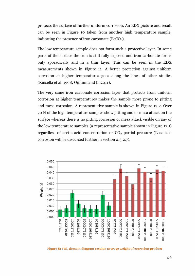
et al. 2010). In Figure 8 the weight of the corrosion product scale of each
condition is displayed. With overall averages of 0.011 and 0.039 g the high
temperature samples developed 3.5 times more scale than the low
temperature ones. After that scale has been developed on the surface, it
protects the surface from further uniform corrosion. A surface layer for a low
and high temperature sample can be seen in Figure 9; acetic acid and pCO2
are the same in both samples, 1000 ppm and 20 bar, respectively. The
images of the surface are representative for low and high temperature
samples and it does not change significantly with varying acetic acid or CO2
concentrations. It can be seen that the high temperature sample forms a very
dense, thick, and protective iron carbonate layer (cubes in Figure 9.4) which
26
protects the surface of further uniform corrosion. An EDX picture and result
can be seen in Figure 10 taken from another high temperature sample,
indicating the presence of iron carbonate (FeCO3).
The low temperature sample does not form such a protective layer. In some
parts of the surface the iron is still fully exposed and iron carbonate forms
only sporadically and in a thin layer. This can be seen in the EDX
measurements shown in Figure 11. A better protection against uniform
corrosion at higher temperatures goes along the lines of other studies
(Kinsella et al. 1998; Ojifinni and Li 2011).
The very same iron carbonate corrosion layer that protects from uniform
corrosion at higher temperatures makes the sample more prone to pitting
and mesa corrosion. A representative sample is shown in Figure 12.2. Over
70 % of the high temperature samples show pitting and or mesa attack on the
surface whereas there is no pitting corrosion or mesa attack visible on any of
the low temperature samples (a representative sample shown in Figure 12.1)
regardless of acetic acid concentration or CO2 partial pressure (Localized
corrosion will be discussed further in section 2.3.2.7).
Figure 8: TOL domain diagram results; average weight of corrosion product
0.000
0.005
0.010
0.015
0.020
0.025
0.030
0.035
0.040
0.045
0.050
0C
5T9
13
0
50
0C
5T9
13
0
10
00
C5
T91
30
0C
10
T91
30
50
0C
10
T91
30
10
00
C1
0T9
13
0
0C
20
T91
30
50
0C
20
T91
30
10
00
C2
0T9
13
0
0C
5T1
15
80
50
0C
5T1
15
80
10
00
C5
T11
58
0
0C
10
T11
58
0
50
0C
10
T11
58
0
10
00
C1
0T1
15
80
0C
20
T11
58
0
50
0C
20
T11
58
0
10
00
C2
0T1
15
80
We
igh
t [g
]

27
Figure 9: SEM images from low (1, 2 - 1000C20T9130) and high (3, 4 -1000C20T11580) temperature samples
1 2
3 4
Figure 10: EDX measurements on a high temperature sample

28
Figure 12: HCT samples; 1 - low temperature (500C20T9130) without localized corrosion
2 - high temperature (500C20T11580) with localized corrosion
1 2
Figure 11: EDX measurements on a low temperature sample on two different spots

29
2.3.2.2. Effect of CO2 partial pressure (pCO2)
The effect of pCO2 isn’t as obvious in Figure 7 as the effect of temperature.
Therefore, the data was rearranged and displayed in Figure 13. It is shown
that both high and low temperature samples follow the same trend with
increasing pCO2.
In the tests without acetic acid (the first three blue and orange columns) the
corrosion rate increases with increasing pCO2. In the case of the low
temperature samples, the average corrosion rate increases over the 7 day
period from 0.47 mm/y to 049 mm/y and 0.64 mm/y for 5 bar, 10 bar and
20 bar pCO2, respectively. A similar increase can be observed for the high
temperature samples where the corrosion rate stays constant for 5 bar and
10 bar at 0.20 mm/y and then increases for 20 bar pCO2 to 0.25 mm/y.
These results are consistent with many other studies where an increase of
pCO2 increases the corrosion rate due to a higher concentration of carbonic
acid and therefore a lower pH in the liquid phase.
Within the tests containing 500 ppm acetic acid (the centre three blue and
orange columns) the corrosion rate slightly decreases with rising pCO2 at low
temperature and basically stays constant for the high temperature testing.
The effect of a falling corrosion rate is even more pronounced with a
1000 ppm acetic acid concentration.
The corrosion rate of the low temperature samples at 1000 ppm decreases
from 0.80 mm/y to 0.66 mm/y and stays more or less constant at
0.67 mm/y with 5 bar, 10 bar, and 20 bar pCO2, respectively. At high
temperature virtually the same decrease of corrosion rate can be observed.
The corrosion rate is 0.43 mm/y, 0.34 mm/y, and 0.35 mm/y for 5 bar,
10 bar, and 20 bar pCO2.

30
Figure 13: TOL domain diagram results; data from Figure 7 presented to show the effect of carbon dioxide
The effect of a declining corrosion rate at the TOL with an increasing pCO2 at
high acetic acid concentration has not been reported before in the literature.
Some publications would even suggest the opposite by saying that a higher
pCO2 decreases the pH in the condensed liquid which in turn locally re-
associates acetic acid which then increases the corrosion rate. This effect is
not observed in the present study.
It can be concluded that an increase in pCO2 without any acetic acid present
results in a decreasing pH of the condensed liquid which results in a more
severe environment and therefore in an increased corrosion rate. This is in
line with previously published data, experimental and predictive.
A different mechanism must come into play at medium and high acetic acid
concentrations. More experiments need to be conducted in similar
conditions with focus on the formation and structure of the protective film
formed. At this stage is can be anticipated that the protective film that forms
at elevated acetic acid concentrations becomes more protective with an
increasing pCO2. This might be the case due to the fact that the negative
influence of a higher pCO2, the lower pH in the condensed liquid, is not as
0.00
0.10
0.20
0.30
0.40
0.50
0.60
0.70
0.80
0.90
0C
5T9
13
0
0C
5T1
15
80
0C
10
T91
30
0C
10
T11
58
0
0C
20
T91
30
0C
20
T11
58
0
50
0C
5T9
13
0
50
0C
5T1
15
80
50
0C
10
T91
30
50
0C
10
T11
58
0
50
0C
20
T91
30
50
0C
20
T11
58
0
10
00
C5
T91
30
10
00
C5
T11
58
0
10
00
C1
0T9
13
0
10
00
C1
0T1
15
80
10
00
C2
0T9
13
0
10
00
C2
0T1
15
80
Co
rro
sio
n R
ate
[m
m/y
]

31
pronounced at higher acetic acid concentrations due to an already low pH in
these conditions. A protective corrosion product layer was observed in
previous studies, even in lower temperatures (Zhang et al. 2007).
2.3.2.3. Effect of Total Acetic Acid
The influence of acetic acid on TOL corrosion rate was observed to be very
strong. Figure 7 clearly displays that within the same CO2 partial pressure
and temperature regime, the corrosion rate increases with increasing acetic
concentration, except for one value which is 0C20T9130. This test was
repeated 5 times and always gives a higher corrosion rate compared to the
tests with acetic acid.
The average of all tests with the same total acetic acid concentration shows
the same trend; the more acetic acid, the higher the corrosion rate (Figure
14). The low temperature tests show an average corrosion rate of 0.54 mm/y,
0.59 mm/y and 0.71 mm/y as an average of 0 ppm, 500 ppm and 1000 ppm
of acetic acid, respectively. High temperature tests give an average corrosion
rate of 0.22 mm/y, 0.30 mm/y and 0.38 mm/y for 0 ppm, 500 ppm and
1000 ppm acetic acid, respectively (Figure 14).
At high temperatures, the corrosion rate correlates linearly with the total
acetic acid concentration. This can be seen by looking at the R-squared value.
R-squared is a statistical tool that indicated how well a trend line, in this case
a linear trend line, fits the values with 0 being no fit at all and 1 being a
perfect fit. The high temperature samples display a perfect linear fit with an
R-squared value of 1. The low temperature tests don’t seem to follow a linear
increase in corrosion rate against acetic acid concentration. It shows a
0.05 mm/y increase from 0 ppm to 500 ppm acetic acid and a 0.12 mm/y
increase from 500 ppm to 1000 ppm acetic acid, resulting in an R-squared
value of 0.9465 (Figure 14).

32
Figure 14: Average corrosion rates of the different acetic acid concentrations at low (LT) and high (HT) temperatures
By calculating the average without the unusually heavily corroded sample
0C20T9130 for the average corrosion rate without acetic acid at low
temperatures a linearity can be observed (Figure 15). The average corrosion
rate would be 0.48 mm/y for no acetic acid and would display an increase of
0.11 mm/y from 0 ppm to 500 ppm acetic acid and a 0.12 mm/y increase
from 500 ppm to 1000 ppm acetic acid. The R-squared value in this case is
0.9994 which is a much better linear fit than the R-squared value of 0.9465
of the previously calculated CR.
Taking these values into consideration, the low temperature samples can be
seen as more susceptible to an increasing acetic acid concentration displayed
by the gradient of the corrosion rate.
The scale formation seems to be also affected by the acetic acid concentration
as displayed in Figure 8. In 4 out of 6 sets (at 20 bar pCO2 and low
temperature and all tests at high temperature) the weight of scale formed on
the samples is the lowest at 0 ppm acetic acid, followed by 1000 ppm acetic
acid and the highest weight of scale is at 500 ppm acetic acid. Most of them
results are within the error bars of the tests, but a trend is clearly visible.
0.54
0.59
0.71
0.22
0.3 0.38
R² = 0.9465
R² = 1
0
0.1
0.2
0.3
0.4
0.5
0.6
0.7
0.8
0 500 1000
Co
rro
sio
n R
ate
[m
m/y
]
Total Acetic Acid Conc. [ppm]
Avrg. CR at LT
Avrg. CR at HT

33
Figure 15: Average corrosion rates of different acetic acid concentrations at low (LT) and high (HT) temperatures, without sample 0C20T9130
2.3.2.4. Effect of Free Acetic Acid
The free acetic acid can be calculated from the total acetic acid and the pH
value (For more information see Equation 9 and Figure 2). The amount of
free acetic acid was therefore calculated using the measured pH of the
samples. Unfortunately, during the beginning of the testing, the pH was not
measured for all tests; therefore not all samples can be evaluated here.
Nevertheless, in Figure 16 the corrosion rates are plotted against the free
acetic acid concentration for those experiments for which data was available.
The blue and orange data points represent low and high temperature
samples, respectively. Symbols of the same colour and shape are taken from
the same test.
As a test progresses, the free acetic acid goes down due to a rising pH in the
bulk solution. The corrosion rate also decreases with the decreasing free
acetic acid over time in an almost linear way. For any given set of conditions
the corrosion rate is higher for a higher free acetic acid concentration, which
is again in line with previous published data (Singer et al. 2004; George and
Nesic 2007; Singer et al. 2009). This goes along with the observation of a
0.48
0.59
0.71
0.22
0.3
0.38 R² = 0.9994
R² = 1
0
0.1
0.2
0.3
0.4
0.5
0.6
0.7
0.8
0.9
0 500 1000
Co
rro
sio
n R
ate
[m
m/y
]
Total Acetic Acid Conc. [ppm]
Avrg. CR at LT
Avrg. CR at HT

34
higher average corrosion rate with an increasing total acetic acid
concentration.
The data also reveal that the HCT TOL corrosion test rig in its current state is
not able to maintain a constant specific free acetic acid concentration.
Corrosion products in a droplet at the TOL constantly fall into the bulk
solution, changing the pH and therefore the free acetic acid concentration.
This could be addressed by slight modifications to the set-up, which will be
discussed further in section 4.2 on page 132 onwards.
Figure 16: Free acetic acid concentration against corrosion rate – high vs. low temperature
2.3.2.5. The effect of bulk pH
The pH in the bulk solution was neither a constant nor a controlled variable
of the test; it was the result of all test parameters and it was constantly
changing throughout every test. The pH at the beginning of each test was
essentially dependent on the acetic acid concentration and the pCO2.
For the iron concentration measurements, a bulk solution sample was taken
every 24 hours. The pH and iron concentration were measured and the
corrosion rate calculated for this sample. Using this data, it was possible to
0
0.2
0.4
0.6
0.8
1
1.2
1.4
1.6
1.8
2
0 200 400 600 800 1000 1200
Co
rro
sio
n R
ate
[m
m/y
]
Free Acetic Acid [ppm]
HT LT

35
correlate an average corrosion rate over 24 hours for a representative pH
range. This range of pH was determined from the measurement at the
beginning and end of each 24 hour period. In Figure 17 (low temperature)
and Figure 18 (high temperature) the corrosion rates are plotted against the
pH range, regardless of what day of the 7 day test period the measurement
was recorded. In the graphs the total acetic acid concentration is
differentiated using different colours.
Regardless of the original total acetic acid concentration and the day of
sampling, both, in the low and high temperature test the corrosion rate
against pH graphs follow almost an exponential decay curve as indicated in
red. Also at both temperatures, comparing tests where acetic acid is present
and absent in the same diagram, it seems that there are numerous outliers in
the tests without acetic acid. Most of the outliers of the low temperature
testing are from first two days of testing 0C20T9130 sample with an
unusually high corrosion rate especially in the beginning of the test.
Nevertheless, the overall picture follows the same trend.
Figure 17: Corrosion rate against pH for all low temperature samples; differentiated only in 0 ppm, 500 ppm and 100 ppm of acetic acid
0
0.2
0.4
0.6
0.8
1
1.2
1.4
1.6
1.8
2
3 3.5 4 4.5 5 5.5 6
Co
rro
sio
n R
ate
[m
m/y
]
pH
0
500
1000

36
Figure 18: Corrosion Rate against pH for all high temperature samples; differentiated only in 0 ppm, 500 ppm and 100 ppm of acetic acid
The pH has a very strong influence on the amount of free acetic acid; with
the data shown in this section, it can be assumed that the corrosion rate is
highly affected by both the pH itself and the resulting decrease of free acetic
acid.
2.3.2.6. Surface Roughness
Using the Infinite Focus Microscope (IFM) it was possible to capture a large
portion of the curved surface and transform it back into a flat area suitable
for further data processing. Surface roughness was calculated but no pattern
was observed in these results. For example, in Figure 19 the results of two
surface roughness measurements are shown. Both measurements are
performed on the same sample on the same spot with a totally different
outcome. The results of Figure 19 are representative for most measurements.
Because all samples are slightly different and the flattening of the surface
worked slightly different for each sample, it was not possible to gather a
representative and comparable roughness values.
0
0.1
0.2
0.3
0.4
0.5
0.6
0.7
0.8
0.9
1
3 3.5 4 4.5 5 5.5 6 6.5
Co
rro
sio
n R
ate
[m
m/y
]
pH
0
500
1000

37
Figure 19: Surface roughness measurements using the IFM, 50x magnified, flattened, in false colours
2.3.2.7. Localized Corrosion
The evaluation for localized corrosion was performed also by means of the
IFM but much more successfully than the roughness measurements. The
localized attack was usually wide and flat bottomed (Figure 20) which allows
easy examination with an optical microscope. Due to issues indicated in the
previous section on “surface roughness” the values should be regarded as an
approximation rather than an exact value of the pit depth.
Temperature has the most dominant effect on localized attacks within the
tested parameters. Of all the samples tested at low temperature, just two
show localized attacks. One sample was exposed to 0 ppm and the other one
to 500 ppm of acetic acid; however, both samples were exposed to a high CO2
partial pressure (20 bar). In both instances, the localized corrosion is very
shallow (< 30 m) and rather wide. The pitting probability for all low
temperature samples is 7 % and therefore very low compared to the high
temperature samples with 70 % pitting probability.
As indicated by the very high pitting probability, much more pitting was
evident at high temperatures. All of the different parameter combinations
showed one or more samples with localized corrosion except for 500 ppm
acetic acid at pCO2 = 10 bar.
In general, the localized attack was also more severe at high temperatures.
The shape of most of the pits was wide with steep walls and a flat bottom, it
Ra: 4.750 m Rz: 29.595 m Ra: 1.900 m Rz: 15.554 m

38
can be considered as mesa corrosion (Nyborg and Dugstad 2003). For mesa
attack to form, a partially protective corrosion product film needs to form,
which is the case at high temperatures in this test (Nyborg 1998). During the
evaluation of the mesa corrosion it was observed that the number of localized
attacks per sample increases with increasing acetic acid concentration
regardless of the pCO2.
The connection of acetic acid and pCO2 to the width and depth of the
localized attacks is not straight forward. Figure 21 plots the average depth of
the localized corrosion attack for each condition. It can be seen that at low
pCO2 (5 bar) the pitting depth is significantly higher with 1000 ppm of acetic
acid compared to 0 ppm and 500 ppm acetic acid. The total opposite effect
was observed at high CO2 partial pressure (20 bar) where the average depth
of the localized corrosion is reduced with increasing acetic acid
concentration. At 10 bar pCO2, the depth of the localized corrosion increased
slightly from 0 ppm to 1000 ppm acetic acid concentration but dropped to 0
m at 500 ppm acetic acid (The occurrence of localized attacks is given as a
pitting probability and therefore it might be coincidental that there is no
pitting).
Figure 22 displays the results from Figure 21 in a rearranged form to
emphasize the effect of pCO2. A very similar trend is visible as seen with the
acetic acid concentration. At 0 ppm acetic acid, the average localized
corrosion depth increases with increasing pCO2, whereas the average depth
decreases at 1000 ppm acetic acid with increasing pCO2. It is also slightly
higher at 500 ppm acetic acid across the range from 5 to 20 bar pCO2.
Regardless of the depth and size, an increase of localized attacks could be
observed with increasing acetic acid concentration within the same CO2
partial pressure range.
There are many contradictory publications available concerning the
influence of acetic acid concentrations and pCO2 at low pressures for BOL
and TOL corrosion (Crolet et al. 1999; Mendez et al. 2005; Nafday and Nesic
2005; Amri et al. 2010; Fajardo 2011). The results indicate that there might
be a more complicated relation between acetic acid, higher CO2 partial

39
pressures, and pitting depth. It is very important to note that there is a
pitting probability, it means that there is a high chance that pitting will
occur, but it is not a pitting certainty. This may lead to the contradicting
results in comparable conditions, especially in laboratory tests which are
usually short in duration.
Figure 20: Example of localized corrosion 1) SEM image 2) IFM image (1.3 mm x 1 mm)
Figure 21: Average depth of the localized corrosion in different conditions; emphasising the effect of acetic acid
0
50
100
150
200
250
HAc: 0 HAc:500
HAc:1000
HAc: 0 HAc:500
HAc:1000
HAc: 0 HAc:500
HAc:1000
Pit
tin
g D
ep
th [
m]
1 2
| pCO2: 5 bar | | pCO2: 10 bar | | pCO2: 20 bar |

40
Figure 22: Average depth of localized corrosion in different conditions; emphasising the effect of pCO2
0
50
100
150
200
250
pCO2: 5 pCO2:10
pCO2:20
pCO2: 5 pCO2:10
pCO2:20
pCO2: 5 pCO2:10
pCO2:20
Pit
tin
g D
ep
th [
m]
| 0 ppm HAc | | 500 ppm HAc | | 1000 ppm HAc |

41
2.4. Conclusions
The corrosion at the TOL is affected by many parameters.
The main influence on TOL corrosion within the investigated
parameters of this study had the pipe temperature. A dense and
protective corrosion layer formed at high temperatures.
Localized attacks were observed regularly at the higher temperatures.
A high CO2 partial pressure (20 bar) has a positive influence at high
acetic acid concentrations (1000 ppm).
A very important parameter is the pH of the bulk solution, which is
directly related to the concentration of free acetic acid. The lower the
pH, the more acetic acid is present in its undissociated state and
therefore increases the corrosion at the TOL.
No localized corrosion was observed for medium pCO2 (10 bar) and
medium acetic acid concentration (500 ppm).
The lowest average depth of localized corrosion of the high
temperature samples was observed for low and medium pCO2 (5 and
10 bar) with no acetic acid as well as for high pCO2 (20 bar) with a
high acetic acid concentration (1000 ppm).
The correlation between higher pCO2 and acetic acid concentrations
on TOL corrosion needs further investigation
Influence on TOL corrosion of
Temperature > acetic acid concentration > pCO2

42
3. Generic Volatile Corrosion Inhibitor
Compound Investigation
3.1. Introduction
3.1.1. CO2 Corrosion Inhibition
Carbon steel is widely used as pipeline steel in the oil and gas industry for a
vast variety of applications. Many of the environments are corrosive for
carbon steel and therefore carbon steel requires protection. There are two
main approaches protecting against CO2 corrosion of carbon steel; corrosion
inhibition or pH stabilisation. Inhibition by pH stabilisation increases the pH
of the formation water to 6.5– 7.5 which facilitates the formation of a
protective iron carbonate layer on the steel surface, reducing Bottom-of-the-
Line (BOL) corrosion considerably (Dugstad et al. 2003). The pH
stabilisation method can be used in combination with glycol to prevent the
formation of hydrate (Dugstad and Dronen 1999). In this way, the pH
stabilising agents can be reclaimed with the glycol and it becomes a more
cost efficient way of inhibition (Halvorsen and Andersen 2003). The limiting
factor for this technique is formation water; it cannot be used with large
quantities of formation water due to the formation of calcium carbonate scale
close to the pipeline inlet at elevated pH levels (Nyborg 2009).
Corrosion inhibition is one of the most common corrosion control methods
for oil and gas production and transportation (Kapusta 1999). The inhibitors
are usually long chained organic compounds. These compounds attach their
polar head to the carbon steel surface and form a physical barrier between
the steel and the corrosive environment. The corrosion inhibitors were
thought to form a mono layer, but more recent studies have shown that
above a critical concentration they can adsorb to the surface in several
“shapes” like spheres, rods, or double layers. The exact mode of adsorption to
the steel highly depends on the type and concentration of the inhibitor (John

43
et al. 2006; Bosenberg et al. 2007). Tests have shown that inhibitors are
effective in quantities as low as 10 ppm (Thomas 2000) and even lower at 0.5
ppm (Jovancicevic et al. 2000). The film formed by many inhibitors is
proven to be very stable and cannot easily be removed at shear stresses
commonly found in pipelines (Xiong et al. 2011).
The corrosion inhibitors are usually applied continuously by injection into
the liquid phase of the pipeline. Consequently, the inhibitors only prevent
corrosion in the liquid phase of the pipeline; therefore they are commonly
referred to as Bottom-of-the-Line inhibitors. The gas phase above the liquid
phase is beyond the influence of normal BOL inhibitors which leads to the
potential risk of Top-of-the-Line (TOL) corrosion in wet gas pipelines.
3.1.2. Top-of-the-Line Corrosion Inhibition
The inhibition of TOL corrosion is a common problem in the transportation
of wet gas. There are several different approaches to the problem.
The best known and longest used inhibition technique is the inhibitor batch
treatment. A batch of inhibitor with a high film persistency is carried through
the pipeline between two PIGs reaching and applying inhibitor to the TOL.
The treatment has to be repeated periodically, otherwise the corrosion
protection will decrease significantly over time (Punpruk et al. 2010). There
are several problems with the batch treatment; not all pipelines are prepared
to launch PIGs or the PIG launcher might be too small for the large volume
of inhibitor required (Gunaltun and Belghazi 2001). Most importantly, the
production has to be shut down to perform the operation which results in a
huge production loss for the operating company.
In 2003, a novel approach using a PIG was presented, the TLCC-PIG
(Gunaltun and Payne 2003). The TLCC-PIG is launched into the pipeline
during production. The gas pressure propels the PIG through the pipeline.
Utilizing the Venturi Effect, the TLCC-PIG sprays the conventionally
inhibited formation water from the BOL to the TOL. The production does not
have to be stopped entirely, which is a major advantage over the
conventional PIGs. Nevertheless, some lines require cleaning before a TLCC-

44
PIG can be run to prevent the nozzles being jammed (Freeman 2009). Also,
the possibility of a TLCC-PIG getting stuck in a pipeline is still present which
would result in a huge loss of production and incur recovery costs.
The best solution to inhibit the TOL would be a continuous chemical
treatment that is able to reach the TOL without the assistance of a PIG.
Modes of transport to the TOL for continuous chemical treatment include
foaming, spreading, and volatility.
Foaming inhibitors are generally not in use because the foam will cause
problems in the processing of the formation water and natural gas or even
require the addition of anti-foaming agents, increasing the total cost.
Nonetheless, solely from the point of corrosion inhibition, published results
indicate that foaming does work in the laboratory as a mode of inhibitor
transport (Jevremovic et al. 2012).
The spreading inhibitor model was mainly researched and published by
Günter Schmitt at al. where a spreading agent was reported to be able to
carry the inhibitor to the TOL against gravity (Scheepers 2001; Schmitt et al.
2001). No literature could be found of a field trial performed using spreading
inhibitors.
Volatile Corrosion Inhibitors (VCIs) are thought to be a promising way
forward of continuous chemical TOL corrosion mitigation. VCIs are injected
into the liquid phase of the pipeline, similar to conventional BOL corrosion
inhibitors. It is believed that the VCIs evaporate and co-condense at the TOL
and inhibit corrosion. Due to their volatility, VCIs are able to reach the entire
surface of the carbon steel pipeline, including complex shaped parts and
crevices (Andreev and Kuznetsov 1998). Unfortunately, VCIs are not as
frequently researched as conventional BOL corrosion inhibitors. Therefore,
the actual mechanism of inhibition of most individual VCI compounds is not
known. Some commercially available VCIs are not even volatile and they
simply stabilize the pH at the BOL. A higher pH at the BOL leaves less
organic acid available for the TOL and therefore less TOL corrosion is
occurring (Gunaltun et al. 2010). BOL pH stabilisation is indeed a way to
mitigate TOL corrosion, but the inhibitor cannot accurately be called a VCI.

45
Reliable field data is also rarely published, and when it is, the identity of the
compounds is often kept confidential (Gunaltun 2006; Pou 2009).
Nevertheless, a paper has been published with an inhibition efficiency of
about 70 % in a field trial (Punpruk et al. 2010). The scarce amount of
information does leave enormous room for improvement and research for
VCIs.
In the following sections, the TOL corrosion inhibition potential of a variety
of amines is investigated by different methods. Amines with a variety of
molecular structures, chemical, and physical properties were chosen to shed
light onto TOL corrosion inhibition by VCIs.

46
3.2. Experimental
3.2.1. Generic Volatile Corrosion Inhibitor Candidates
Different potential generic VCI compounds were investigated for their ability
to inhibit TOL corrosion (Table 3). Some of the VCIs were chosen because
they are used in VCI applications outside the oil and gas industry. Some
others were already used in commercially available VCIs in the oil and gas
industry but were never thoroughly investigated. Again others were chosen
due to their similarity in molecular formulation (small amino molecules) or
physical properties (e.g. boiling point) (Bastidas et al. 1990; Petersen et al.
2004; Bhargava et al. 2009).
All 16 generic VCIs are amines or feature amine functional groups and
therefore they are all bases. Amines of different classes were chosen
including primary-, secondary-, tertiary- and cyclic amines. Some of the
generic VCIs also have the characteristic of a combination of the classes
mentioned. An extreme example combining all classes is
1-(2-aminoethyl)piperazine. It has three nitrogen atoms; a primary, a
secondary and a tertiary one in a form of a ring (cyclic) with a tail. A graphic
illustration of the different classes and their typical chemical structures can
be found in Table 4. Dark grey atoms represent Carbon (C), small light grey
atoms are Hydrogen (H), blue atoms are Nitrogen (N) and red atoms are
Oxygen (O) in all graphics used hereafter.
The results of all compounds in every test are duplicated. If the results are
not satisfactory, a triplicate was conducted. The numeric value presented for
each individual test is the average of successful tests. It was deemed not
practical to show individual error bars in the diagrams since it would either
clutter the diagram in its current state or it would have been necessary to
show the results individually, which in turn would have multiplied the
amount of diagrams approximately by 8. Additional to the vast amount of
diagrams, it would have made a visual comparison between the individual
VCIs much harder, if not impossible.

47
A list of the investigated generic VCIs including their molecular formula can
be found in Table 3. A table with the basic physical and chemical properties
and a basic description for each compound can be found in the results and
discussion (in section 3.3.2, Table 11 and in section 3.3.3, Table 16) for the
respective compound. All compounds were sources from Sigma Aldrich
where also all the MSDS sheets can be accessed.
The GVCIs were tested using a variety of test setups to investigate their TOL
and BOL inhibition properties. Most of the generic VCIs underwent all tests,
but some limitations apply due to a shortage of generic VCI or equipment
usability. The different testing procedures will be described in the following
sections.
Table 3: List of GVCIs investigated
Name Formula
1-(2-Aminoethyl)piperazine C6H15N3
4-Aminomorpholine C4H10N2O
Aniline C6H7N
Benzylamine C7H9N
Cyclohexylamine C6H13N
Diethylamine (DEA) C4H11N
Dicyclohexylamine C12H23N
N,N-Dimethylethylamine (DMEA) C4H11N
N-Methyldiethanolamine (MDEA) C5H13NO2
4-Methylmorpholine C5H11NO
Methylpiperazine C5H12N2
Morpholine C4H9NO
Octylamine C8H19N
4-Picoline C6H7N
Pyridazine C4H4N2
Pyridine C5H5N

48
Table 4: Graphic illustration of the different types of amines
Example Formula Straight Molecule Cyclic Molecule
Primary Amine
NH2
Secondary Amine
NH
Tertiary Amine
N
3.2.2. Horizontal Cooled Tube (HCT) Test
Most of the experimental procedures and materials used to evaluate VCIs
using the HCT test setup are identical to the procedures and materials used
to develop the TOL domain diagram. Therefore, detailed information about
the pressure reactor, corrosion samples, preparation of a test, and corrosion
rate determination can be referred back to the experimental section of the
previous chapter (Section 2.2 Experimental).
3.2.2.1. VCI Charging Process
A 150 mL high pressure liquid charging pipette manufactured by Swagelok
was used to insert the VCI into the pressurized reactor. A tedious procedure

49
had to be followed to maintain the lowest possible oxygen contamination in
the test chamber.
High purity CO2 was connected to the top of the pipette (1). All valves were
opened and CO2 gas flowed through the pipette to remove oxygen. After a
few minutes, the tube fitting (4) was attached to the valve of the pressure
reactor while gas was still flowing through. After the tube fitting was
connected to the valve of the pressure reactor, the lower valve of the high
pressure pipette (3) was closed, leaving the tube (between 3 and 4) slightly
under pressure but free of oxygen. Then, the pressure from the rest of the
pipette was released and the CO2 was disconnected and the top valve (2) was
removed from the pipette. 100 mL of a pre-sparged 0.1 % NaCl solution and
1000 ppm of the VCI (0.75 mL) was inserted into the pipette and sparged for
10 minutes using high purity CO2. After the 10 minutes of sparging, the
sparge tube was removed and the top valve (2) was reattached to the pipette.
The reattachment of the valve was the only step where a very small amount
of oxygen ingress might have occurred. Then the CO2 line was reconnected
(1) and the pipette was pressurized to a higher pressure as the TOL test
reactor. The lower valve (3) was opened, than the valve at the TOL test
reactor was opened and the whole volume of the pressure pipette was
transferred into the TOL test reactor.
After the process, a sample of the bulk solution was taken to have a baseline
reading of iron from the bulk solution at the moment the VCI was inserted.
Figure 23: Liquid charging pipette
1 2 3 4

50
3.2.2.2. Test Conditions
The test conditions used for generic VCI testing can be seen in Table 5. All
test parameters were kept constant throughout all generic VCI tests to allow
maximum comparability.
Table 5: Test conditions for generic VCI testing using the HCT test
Test duration 7 days (approx. 160 h)
Pre-corrosion 1 day (approx. 20 h)
Bulk solution 750 mL 0.1 % NaCl
Condensation rate 0.4 g/m2/s
Total pressure/pCO2 @ Troom 20 bar (290 psi)
Acetic acid conc. 1000 ppm
VCI conc. 1000 ppm
Temperature regime 91 ⁰C Tautoclave
30 ⁰C Tsample
3.2.3. Cooled Finger Probe (CFP) Test
The CFP approaches the testing of VCI from a totally different angle. Tests
are performed under ambient pressure using a combination of corrosion
under TOL conditions and electrochemistry in the condensed liquid. The test
method was developed and performed at Nalco Energy Solutions in
Singapore (Gough et al. 2009).
3.2.3.1. CFP Corrosion Sample and Conditions
The CFP test chamber is a slightly modified 2 L glass cell and a glass head
with jointed fittings (Figure 24). Water saturated CO2 was constantly sparged
into the cell though the bulk solution which consisted of a 0.1 % sodium
chloride solution with 1000 ppm acetic acid. The exiting CO2 flowed through
a bubbler to maintain ambient pressure and prohibiting oxygen from
entering the cell. The bulk solution was heated using a hot plate connected to
a thermocouple in the solution to control the solution temperature.

51
An externally cooled LPR probe was used for testing. Three 1018 grade
carbon steel pins (ASTM-A29 2011) were attached to the LPR probe and
subsequently cleaned for an hour in a cleaning alcohol. The carbon steel pins
were commercial test samples commonly used for this type of probe and for
each test a new set was used.
The LPR probe was suspended over a beaker inside the class cell. Liquid
condensed at the three carbon steel pins corroding them under TOL
conditions for 22 hours a day. The condensed liquid was then collected in the
beaker. For 2 hours a day, the LPR probe was immersed into the collected
condensed liquid in the beaker and LPR scans were performed using a
Gamry Reference 600 potentiostat. The carbon steel pins are 4.75 mm in
diameter and 30.5 mm long resulting in a total surface area for all three pins
of 14.03 cm2.
After the LPR scans were performed, the condensed liquid was sampled from
the beaker. It was analysed for acetic acid (by means of gas chromatography),
iron concentration (by means of a Hach spectrophotometer), and pH. Every
48 hours, a 25 mL sample from the bulk solution was taken and also
analysed for acetic acid, iron and pH. Any liquid that was removed from the
cell in any way was replenished into the bulk liquid with a pre-sparged
0.1 % sodium chloride, 1000 ppm acetic acid solution.
The CR calculated by means of LPR and IC does not necessarily give the
same values of CR because different corrosion mechanisms are responsible
for the corrosion. LPR essentially just measures the corrosivity of the
condensed liquid after the 22 hours of TOL corrosion. The CR by means of IC
on the other hand, is directly affected by severity of the TOL corrosion which
is, in turn, highly affected by the condensation rate. Nevertheless, both
follow the same trend indicating whether or not a VCI compound has
inhibiting properties, which can be seen in the “Results and Discussion”
section.
In addition to the LPR tests and iron concentration (IC) measurements, the
corrosion rate was also determined by means of weight loss of the carbon
steel pins.

52
The acetate concentration was determined by means of ion chromatography.
With the acetate concentration and the pH it was then possible to calculate
the concentration of the dissociated and undissociated acetic acid; in other
words, how much of the measured acetate is present in the solution as acetic
acid and therefore contributes to TOL corrosion (more in section 2.1.3).
Equation 9
The test duration was 7 days, where the first two days were dedicated to a pre
corrosion of the sample under TOL conditions but without VCI in the system.
After the two days of pre-corrosion, the generic VCI compound was inserted
into the bulk solution.
As the condensed liquid removed from the cell, the condensation rate was
calculated daily and was found to be between 0.25 g/m2/s and 0.40 g/m2/s
using the following equation:
Equation 13
where m is the mass of condensed liquid in kilograms, A the sample area in
square meters and t is the time in seconds over which the condensation
occurs (here 22 hours = 79200 s).
Table 6: Test conditions for the cooled finger probe tests
Test duration 7 days (approx. 160 h)
Pre-corrosion 2 day (approx. 48 h)
Bulk solution 850 mL 0.1 % NaCl
Condensation rate 0.25 – 0.40 g/m2/s
Total pressure Ambient
pCO2 ~50 ml/min
Acetic acid conc. 1000 ppm
VCI conc. 1000 ppm
Temperature regime 80 ⁰C TBulk
0 ⁰C TCoolant

53
Figure 24: Image and schematic of the Cooled Finger Probe test set up

54
3.2.4. Altered Horizontal Cooled Tube (A-HCT) Test
An alternative version of the HCT test was invented to minimize the effect of
the VCI on the pH of the bulk solution. In this way, the volatility and
inhibition effect directly at the TOL can be investigated.
To achieve this objective, two stainless steel cups were attached to the inside
of the reactor. A schematic and a photograph are shown in Figure 25. The top
cup is designed to collect any condensation and corrosion product to prevent
it from mixing with the bulk solution and altering the pH. The lower cup
holds a VCI solution and separates the VCI from the bulk solution, again to
prevent any changes in pH. The lower cup is partly submerged in the bulk
solution to maintain the same temperature. The VCI concentration of
1000 ppm is calculated by means of the total solution in the pressure reactor.
It takes the 750 mL of bulk solution as well as the 100 mL of solution in the
lower beaker into account, totalling 850 mL. Therefore, 0.85 mL of VCI was
inserted in the lower beaker.
The contents of the top cup were removed daily and a 10 mL bulk solution
sample was taken at least every second day. Both samples were analysed for
their iron concentration by means of AAS and the pH was measured.
The bulk solution and condensed liquid samples are drawn by opening the
valve of the autoclave and the high pressure inside the autoclave forces the
fluid out. Because of large sample sizes (approx. 85 mL per day) and
therefore large pressure drop, the internal pressure was topped up to the
original pressure of the autoclave after two days. The test conditions for the
A-HCT testing are displayed in Table 7.

55
Table 7: Test conditions for generic VCI testing using the A-HCT test
Test duration 5 days (approx. 90 h)
Pre-corrosion No pre-corrosion
Total liquid in vessel 850 mL 0.1 % NaCl
Condensation rate 0.4 g/m2/s
Total pressure/pCO2 @ Troom 20 bar (290 psi)
Acetic acid conc. 1000 ppm
Total VCI conc. 1000 ppm
Temperature regime 91 ⁰C TAutoclave
30 ⁰C TSample
Figure 25: Schematic and photograph of the A-HCT test setup

56
3.2.5. Rotating Cylinder Electrode (RCE) Test
RCE tests were performed to investigate the inhibition effect of the VCI on
the BOL corrosion. The aim also was to investigate the mechanism of
inhibition for the given VCIs.
500 mL of a 0.1 % NaCl solution with 1000 ppm of acetic acid was used to
perform all electrochemical tests. The solution was pre-sparged for about
60 minutes with CO2 and continuously sparged throughout the test at a rate
of approximately 50 ml/min. A silver silver-chloride reference electrode and
a platinum mesh counter electrode were used in each test. Low rotation
speeds of 200 rpm were used throughout the testing (Figure 26).
A 1030 grade carbon steel sample with a density of 7.87 g/cm3 was used as
the RCE sample. Samples were machined from a rod and subsequently
stored in a desiccator until they were used. It was wet ground using water
with 120, 320 and 600 grit silicon carbide grinding paper and rinsed with
water and acetone. Afterwards, it was put into a beaker containing acetone
and sonicated in the ultrasonic bath for 10- 15 minutes. Then, it was rinsed
again with fresh acetone, dried, and screwed onto the RCE sample holder
between two Teflon washers to prevent crevice corrosion. The diameter and
height were measured to calculate the sample area (approximately 3 cm2)
and the test was started.
A Gamry Reference 600 potentiostat with Gamry software was utilized to run
a test sequence consisting of an open circuit potential (OCP) for 30 minutes,
followed by alternating linear polarisation resistance (LPR) scans and
electrochemical impedance spectroscopy (EIS), and finally a
potentiodynamic (PD) scan. The entire test duration was 18 hours.
1000 ppm of VCI was inserted into the system after 4 or 5 LPR and EIS tests
(approximately 4 hours) to record the blank corrosion rate for every sample.
The pH was measured right before and after the VCI was inserted. Two
different approaches have been tested for every VCI sample:
- After the pre-corrosion the VCI was injected into the solution. The
VCI raises the pH of the solution and inhibits the corrosion of the steel

57
sample. The overall inhibition performance of the VCI was verified in
this way.
- In other tests, the VCI was also injected into the bulk solution after the
pre-corrosion. The difference was that the pH was adjusted back to a
value before the VCI was inserted into the system (pH 3.20) using HCl
and NaOH. In this way, the inhibition by neutralisation was
eliminated and the ability of the VCI to inhibit by a different
mechanism was investigated. It can be assumed that the residual
inhibition mechanism was due to film forming.
In the following “Results and Discussion” section both results are
distinguished by the addition “+ HCl”.
It was possible to determine the ratio of inhibition by film forming
(Inhibition efficiency of the pH adjusted tests “+HCl”) and neutralisation
(difference in inhibition efficiency of pH adjusted and non-adjusted tests).
Inhibition efficiency will be introduced in section 3.2.7.
Figure 26: Rotating cylinder test set up

58
3.2.5.1. Linear Polarisation Resistance (LPR)
The OCP was allowed to stabilize for 30 minutes before LPR measurements
were initiated. The LPR was measured ±10 mV around the OCP with a scan
rate of 0.125 mV/s. Beta A and Beta C values of 0.12 were assumed
(Ogundele and White 1986) to calculate the Stern-Geary constant (B) of
26.05 using the following equation
Equation 15
The calculated Stern-Geary constant was then used to calculate the corrosion
current density icor in the following equation
Equation 16
where Rp is the polarisation resistance measured in the LPR test.
An example of a LPR scan is displayed in Figure 27. The polarisation
resistance RP has to be gained out of each of the LPR plots to calculate the
icorr using Equation 16. icorr is then used to calculate the CR in Equation 17.
Equation 17
where K1 is a constant of 3.27 *10-3 mm g/A cm y, the constant is needed
that the resulting CR is given in mm/y, icor is the corrosion current density
in A/cm2, the density of the material in g/cm3, in this case 7.87 g/cm3,
and 27.92 was used as the equivalent weight (EW) (ASTM-G102-89 2010).
The calculated CRs are then plotted as a function of time to evaluate the
VCIs. It is possible to run subsequent tests because LPR is essentially a non-
destructive technique (Fontana and Staehle 1980; Enos 1997; Mansfeld
2005).

59
Figure 27: Linear polarisation resistance (LPR) plot of the blank sample – 500 mL of 0.1 % NaCl solution with 1000 ppm acetic acid at 200 rpm
LPR is not able to distinguish between charge transfer resistance and
solution resistance and is better suited for solutions with a high conductivity
(and therefore low solution resistance). To verify the LPR results, EIS
measurements were performed using the RCE test set up.
3.2.5.2. Electrochemical Impedance Spectroscopy
After an initial LPR test a subsequent EIS test was performed (both, LPR and
EIS were continuously alternated). EIS measurements were performed
between 10000 Hz and 0.01 Hz frequency with an AC voltage of 10 mV rms
and 10 points/decade were recorded. The focus of the investigation was on
the Nyquist plot (Figure 28). The advantage of EIS is the possibility to clearly
distinguish between solution resistance (RS) and charge transfer resistance
(RCT) where RS should not be incorporated in the calculation of the CR.
Figure 28 is an actual blank EIS measurement of the investigation. It can be
seen that the solution resistance is quite high, but more on this topic in the
Results and Discussion of this chapter.
ZView software (Scribner Associates Inc.) was used to extract RS and RCT
from the recorded data. The CR was then calculated using Equation 15,
-0.675
-0.67
-0.665
-0.66
-0.655
-0.65
-4.00E-05 -2.00E-05 0.00E+00 2.00E-05 4.00E-05
Po
ten
tial
[V
vs.
Re
f.]
Current Density [A/cm2]

60
Equation 16, and Equation 17. All results are displaying the evolution of the
CR over time and no single EIS plots are shown anymore.
Figure 28: EIS (Nyquist) plot of the blank sample – 500 mL of 0.1 % NaCl solution with 1000 ppm acetic acid at 200 rpm
3.2.5.3. Potentiodynamic Scan
At the end of each test sequence a potentiodynamic scan was performed from
-250 mV to +500 mV around the OCP with a scan rate of 0.167 mV/s.
3.2.6. Corrosion Rate
All TOL corrosion test methods feature two or more ways to determine the
CR of the samples. In all cases, the CR was calculated by means of weight
loss (WL) and by means of the iron concentration (IC) in the solution. In the
case of the CFP, LPR measurements were used as an additional method to
calculate the corrosion rate. The formulas used to calculate the CR by WL
and IC can be found in section 2.2.3 on page 15 “Corrosion Rate
Determination”. To calculate the CR by means of LPR and EIS the Equation
15, Equation 16, and Equation 17 were used.
-30
-25
-20
-15
-10
-5
0
0.00 20.00 40.00 60.00 80.00 100.00
Z"
Z'
RS RCT

61
3.2.7. Inhibition Efficiency
The inhibition efficiency (IE) was calculated for every compound in every
TOL corrosion test. The higher the IE, the more efficient the inhibitor works.
It is calculated by the following equation:
Equation 18
with IE given in percent (Durnie et al. 2001). The unit of CR is irrelevant as
long it is used consistently; here mm/y was used.
To calculate the IE the pre-corrosion values were not taken into account for
electrochemical (LPR and EIS) and iron count data. Technically, the longer a
pre-corrosion would last, the lower the IE of an inhibitor would be. By not
taking the pre-corrosion into account, this effect can be eliminated and the
IE data is more representative for the individual generic VCI compound.

62
3.3. Results and Discussion
In this section, the performance of the individual GVCI compounds will be
discussed separately for each test setup. Due to the vast amount of
compounds and test methods corresponding results to discuss, they were
split into two groups based on their overall performance.
The bottom 8 performing TOL corrosion inhibitors will be discussed in a
group and the focus will be on some key attributes of the different
compounds.
The top 8 performing TOL corrosion inhibitors will be discussed individually
for each test set up. The aim is to propose a mechanism of inhibition for each
compound.
All VCIs are compared to the respective blank test for each set up which will
be presented in the following section.
3.3.1. Blank Test – No Inhibitor
To define an uninhibited CR, blank tests for each set up were performed. The
blank tests were identical to all following VCI tests except for the insertion of
the actual VCI into the system. All upcoming inhibitor efficiency (IE)
measurements will refer to the blank test of the respective set up.
3.3.1.1. Horizontal Cooled Tube - Blank
The results for the blank test in the HCT test can be seen in Table 8 and
Figure 29. The CR during the first two days is around 1.5 mm/y and falls on
day three to approximately 0.6 mm/y where it plateaus until the end of the
test. This is a huge drop for an uninhibited system. The main reason for the
declining CR is the neutralization of the bulk solution via the iron corrosion
product in the droplets which reduces the volatile amount of acetic acid and
therefore the amount of acetic acid available for TOL corrosion.
Nevertheless, the average corrosion rate by weight loss is 0.84 mm/y and via

63
iron concentration it is 0.71 mm/y. The weight loss via iron concentration
does not include the first day, which explains the slightly lower average CR.
The relationship between the pH of the bulk solution and the CR at the TOL
becomes clear in Figure 29. The CR is the highest during the first 48 hours of
the test (above 1.4 mm/y), during this time the pH increases rapidly from
pH 3.2 to pH 4.5. As the pH is above 4.5, the CR drops down to
approximately 0.5 mm/y and stays rather constant while the pH still rises,
but not as fast as in the beginning.
The blank CR and pH graphs will be in displayed in the diagrams of the VCIs
for the purpose of comparison in a grey colour. The blue line is a “trend line”
to highlight development of the data points over time. The average CRs will
be used to calculate the IE of the VCIs.
Table 8: Corrosion rates and inhibition efficiencies from the blank HCT test
Iron conc. (IC) Weightloss (WL)
CR [mm/y] 0.71 0.84
IE [%] - -
Figure 29: Corrosion rate by iron concentration, pH, and corrosion rate trend line from the HCT blank test (without VCI)
0.0
1.0
2.0
3.0
4.0
5.0
6.0
0.0
0.2
0.4
0.6
0.8
1.0
1.2
1.4
1.6
1.8
2.0
0 24 48 72 96 120 144 168
pH
Co
rro
sio
n R
ate
[m
m/y
]
Time [h]
Blank CR-IC Blank pH Linear (Blank CR-IC)

64
3.3.1.2. Cooled Finger Probe - Blank
The blank results for the corrosion test using the CFP are displayed in Figure
30. The CR by means of LPR is higher throughout the test compared to the
CR by means of the IC (as described in section 3.2.3.1). Both, the CR by
means of LPR and IC follow the same trend though. They slightly decline
during day 1-4 and stay levelled at about 0.8 mm/y and 0.4 mm/y,
respectively.
The yellow curve in Figure 30 is the calculated condensation rate for the
respective time period. It stays fairly constant throughout the entire test. The
condensation rate slightly increases from day 2 to day 3 which can
immediately be seen in the CR by means of IC, which decreases at a slower
rate compared to the day before or day after. It is well documented in the
literature that the condensation rate has a strong effect on the CR at the TOL.
At high condensation rates the corrosion product containing droplet is
diluted quickly by condensing liquid, which in turn, makes it hard form a
protective corrosion product layer since it the iron super saturation level
cannot be reached.
In Figure 31 the pH of the bulk solution and the condensed liquid are
displayed. The pH of the bulk solution stays very constant around pH 3. The
pH of the bulk solution stays throughout the experiment because, in contrast
to the HCT test (Section 3.3.1.1) because the condensed liquid with the
corrosion product are collected in an isolated beaker totally separating bulk
solution and condensed liquid. The pH of the condensed liquid also stays
relatively constant but slightly declines from pH 5.3 on the first day to pH 4.9
on the last day.
The CR by weight loss and average CRs by means of LPR and IC are shown in
Table 9. The pre-corrosion was not taken into account for CR by LPR and IC
to be able to calculate the true IE in the later tests.
The curves in Figure 30 and Figure 31 will be displayed in grey in all
upcoming graphs of VCI compounds and the values of Table 9 will be used to
calculate the IE for the VCI compounds.

65
Table 9: Corrosion rates and inhibition efficiencies from the CFP blank test
LPR Iron conc. (IC) Weightloss (WL)
CR [mm/y] 0.78 0.40 1.98
IE [%] - - -
Figure 30: Corrosion rate and condensation rate of the blank sample from the A-HCT test
Figure 31: pH of the bulk solution and condensed liquid of the blank sample from the A-HCT test
0.0
0.2
0.4
0.6
0.8
1.0
1.2
1.4
1.6
0 24 48 72 96 120 144
Time [h]
Blank CR-LPR [mm/y]
Blank CR-IC [mm/y]
Condensation Rate [g/m2/s]
0
1
2
3
4
5
6
7
0 24 48 72 96 120 144
pH
Time [h]
Blank pH Cond.
Blank pH bulk

66
3.3.1.3. Altered Horizontal Cooled Tube – Blank
The blank CR of the A-HCT test slightly decreases from day 1 to day 2 from
1.5 to 1.4 mm/y but then increases again up to 1.9 mm/y by the end of the
test as seen in Figure 32. The development of the CR correlates very well with
the measured condensation rate which essentially stays constant on day 1
and 2 around 0.4 g/m2/s but then increases up to 0.6 g/m2/s. This increase
of condensation rate might be explained with the decrease of pressure due to
the sampling process. The observed increase in CR generated by an increase
in condensation rate goes along with a similar observation in the blank test
of the CFP in section3.2.3.1 Therefore, the close relationship of condensation
rate and CR is witnessed in two blank tests in different test set-ups.
Figure 33 shows that the pH of the bulk solution and condensed liquid stay
constant over time. The bulk solution increases from pH 3.3 to 3.6 whereas
the pH of the condensed liquid decreases from pH 6.1 to pH 5.8.
The average CRs are listed in Table 10. As with the other test methods, the
average CRs are used to calculate the IE for the VCI compounds and the
necessary blank curves will be displayed in grey for a good comparison.
Table 10: Corrosion rates, inhibition efficiencies and scale from the blank A-HCT test
Iron conc. (IC) Weightloss (WL)
CR [mm/y] 1.61 1.31
IE [%] - -

67
Figure 32: Corrosion rate and condensation rate from the blank A-HCT (without VCI)
Figure 33: pH of the bulk solution and condensed liquid from the A-HCT blank sample
0.0
0.5
1.0
1.5
2.0
2.5
0 24 48 72 96
Time [h]
Blank CR-IC [mm/y]
Condensation Rate [g/m2/s]
0
1
2
3
4
5
6
7
0 20 40 60 80 100
pH
Time [h]
Blank pH cond. Blank pH bulk

68
3.3.1.4. Rotating Cylinder Electrode
The blank CRs by means of LPR can be seen in Figure 34 as the scatter
diagram. Two different tests were conducted; the first test was left alone
from beginning to end (black graph labelled ‘Blank - LPR’) and in the second,
the pH was slightly adjusted to pH 3.20 after 5 hours using HCl. The
adjustment was later performed with all VCIs as well to eliminate the
neutralising effect of the VCI to the solution.
In both blank tests, the CR stays constant over the entire test period at
around 1.0 mm/y. The pH at the start of both experiments was 3.25 and at
the end of the blank test, it was 3.48. The slight increase in pH was due to the
corrosion products in the solution. These curves are used as reference for
later LPR measurements.
LPR measurements were alternated with EIS measurements throughout the
tests. The EIS results for the blank tests can also be seen in Figure 34 as line
curves. Both blank tests show a CR of around 2.5 mm/y. It can be seen that
the CRs calculated by means of EIS are about 2.5 times higher than the CRs
calculated by LPR. As explained in the
LPR is not able to distinguish between charge transfer resistance and
solution resistance and is better suited for solutions with a high conductivity
(and therefore low solution resistance). To verify the LPR results, EIS
measurements were performed using the RCE test set up.
Electrochemical Impedance Spectroscopy section 3.2.5 before, EIS can
differentiate between RP and RS and therefore calculates a more exact CR
where LPR includes RS to RP resulting in a higher resistance and therefore
lower CR. Nevertheless, LPR is a standard method to determine the CR in
the field and laboratory which will therefore be continued throughout the
VCI investigation as comparison.

69
Figure 34: LPR and EIS results from the blank RCE tests with (red) and without (black) pH adjustment
A potentiodynamic scan from -0.25 to + 0.5 V around the OCP was
performed at the end of every test procedure. The scans can be seen below in
Figure 35 with an Ecorr of -0.67 V for the blank and 0.63 V the blank with HCl
sample. The potentiodynamic scans of the VCIs will be compared to the
respective blank tests.
Figure 35: Potentiodynamic scan from the blank RCE tests with (red) and without (black) pH adjustment
0
0.5
1
1.5
2
2.5
3
3.5
4
0 5 10 15 20 25 30 35
Co
rro
sio
n R
ate
[m
m/y
]
Time [h]
Blank EIS Blank EIS - HCl
Blank LPR Blank LPR - HCl
1E-08
0.0000001
0.000001
0.00001
0.0001
0.001
0.01
0.1
1
-1 -0.8 -0.6 -0.4 -0.2 0
Cu
rre
nt
[A]
Potential [V]
Blank Blank HCl

70
3.3.1.5. Conclusion on the Blank Tests
The Blank tests are going to be used as a baseline and reference for all tests
including VCIs. For the blank TOL corrosion samples, it can be concluded
that the CR is very responsive to the condensation rate. An impact of the
condensation rate on the CR was observed in two tests, the CFP and the A-
HCT test, which are also the only tests where the condensation rate is being
monitored.
CR rate values of LPR and EIS tests do not match well in the blank test.
Nevertheless, both techniques indicate a stable CR over time in the blank
tests. Since LPR is a standard test in many laboratories, both techniques will
be continued to investigate the VCIs and the electrochemical techniques.

71
3.3.2. Low performing VCIs - Results
In the following section, 8 of the generic VCI compounds will be discussed.
These 8 compounds were the compounds with the lowest performance in
regards of TOL corrosion inhibition. The molecular structures (displayed
using the free molecule editor software Avogadro 1.0.3) and some of the
basic properties of each molecule can be found in
Table 11. The properties of the molecules were taken from the respective
MSDS sheets accessed via the homepage of the supplier, Sigma Aldrich
(MSDS 2009; MSDS 2010; MSDS 2011; MSDS 2011; MSDS 2012; MSDS
2012; MSDS 2012; MSDS 2012).
The molecular structure is displayed as grey, blue, red, and small light grey
spheres representing carbon, nitrogen, oxygen, and hydrogen, respectively.
All of the compounds are amines or involve an amino group. Amino groups
can be found either as primary, secondary, tertiary, cyclic amino group, or in
any combination. Within the compounds discussed in this section,
aminomorpholine is the only molecule that contains an oxygen atom.
The grey graph in every diagram represents the blank test and every VCI
compound has its designated colour/marker combination throughout the
entire “Low performing VCI” discussion.

72
Table 11: Structures and properties of all low performing VCI compounds
Aminoethyl-piperazine
Amino-morpholine
Aniline Dicyclo-
hexylamine
Formula C6H15N3 C4H10N2O C6H7N C12H23N
Molecular weight [g/mol]
129.2 102.14 93.13 181.32
Boiling point [⁰C]
218-222 168 184 256
Vapour pressure [mm Hg]
0.076
(@ 20 ⁰C)
1.65
(@ 25 ⁰C)
1.00
(@ 35 ⁰C)
0.034
(@ 25 ⁰C)
Purity [%] 99 97 99 99
Molecular Structure
Octylamine Picoline Pyridazine Pyridine
Formula C8H19N C6H7N C4H4N2 C5H5N
Molecular Weight [g/mol]
129.24 93.13 80.09 79.1
Boiling
point [⁰C] 175-177 145 208 115
Vapour pressure [mm Hg]
1.00
(@ 20 ⁰C)
4.00
(@ 20 ⁰C)
2.33
(@ 25 ⁰C)
18.00
(@ 25 ⁰C)
Purity [%] 99 99 98 99
Molecular Structure

73
3.3.2.1. Horizontal Cooled Tube
The HCT was used as a first evaluation of the VCIs. Due to a very limited
availability, aminomorpholine was not tested in the HCT test.
The evolution of the CR over time is displayed in Figure 36. It is visible that
all VCIs follow more or less the same pattern of CR over time, except for
three candidates. The majority of the VCI candidates significantly decrease
the CR as soon the VCI was inserted into the autoclave. Nevertheless, tests
that involve picoline, pyridazine or pyridine do not follow the pattern
mentioned before. The CR of the test including pyridine declines slightly
after it was inserted, but levels out around 0.80 mm/y and even increases on
the last day. A very similar trend is shown by picoline and pyridazine except
that CRs for both decrease only during the last day. All three compounds
show a negative IE by means of WL and a very weak or even negative IE by
means of IC (
Table 12). The neutralisation curves of these three VCIs couldn’t be more
different as seen in Figure 37. Pyridazine has the weakest neutralisation
effect on the bulk solution of all tested VCIs (from pH 3.3 to pH 4.1), whereas
picoline and pyridine belong to the VCIs with the greatest neutralising effect
with an increase to pH 5.2 and pH 4.9, respectively (blank pH 3.5).
Within the group of the low performing VCIs aminoethylpiperazine, aniline,
dicyclohexylamine, and octylamine were among the better performers in the
HCT test set up. All tests follow the same trend in which the CR drops
directly after the VCI was inserted into the system. Aminoethylpiperazine
and dicyclohexylamine manage to drop the CR by IC to 0.74 mm/y and
0.60 mm/y on the day after insertion, respectively. Both VCIs maintain a CR
around 0.50 mm/y from day 3 until the end of the test. Aniline and
octylamine follow a very similar trend but show greater fluctuation from day
3 to the end. The average CR by means of IC decreases through the VCIs
aminoethylpiperazine, aniline, dicyclohexylamine and octylamine to
0.59 mm/y, 0.52mm/y, 0.50mm/y to 0.47 mm/y, respectively (
Table 12) compared to a blank CR of 0.71 mm/y. The same trend can be seen
with the CR by means of WL.

74
Aminoethylpiperazine achieves the highest pH neutralisation of the bulk
solution but performs as the worst VCI in this group of four. Straight after
injection the pH increases to pH 5.5 and at the end of the experiment is was
at pH 5.9. The three other VCIs, aniline, dicyclohexylamine, and octylamine
all affect the pH of the bulk solution the in a similar way. Straight after
insertion, the pH of all three is around 4.6, and at the end of the test, the pH
ends up around 5.1.
Table 12: Corrosion rates and Inhibition efficiency by weight loss and iron count from the HCT test
CR [mm/y] IE [%]
IC WL IC WL
Aminoethylpiperazine 0.59 0.75 18 12
Aniline 0.52 0.71 27 17
Dicyclohexylamine 0.5 0.64 30 25
Octylamine 0.47 0.54 34 36
Picoline 0.66 1 7 -22
Pyridazine 0.61 1.6 15 -88
Pyridine 0.96 1 -35 -21
Blank 0.71 0.84 - -
Figure 36: Corrosion rates from the HCT test – VCI was injected right after the first measurement
0.0
0.2
0.4
0.6
0.8
1.0
1.2
1.4
1.6
1.8
2.0
0 24 48 72 96 120 144 168
Co
rro
sio
n R
ate
[m
m/y
]
Time [h]
Aminoethylpiperazine Aniline
Dicyclohexylamine Octylamine
Picoline Pyridazine
Pyridine Blank

75
Figure 37: pH evolution of the bulk solution from the HCT test
3.3.2.1.1. Conclusions from the Horizontal Cooled Tube Test
Most of the tested VCIs display their very good ability of neutralisation in
this test. All VCIs increase the pH straight away. None of the tested
compounds displays good inhibition ability in this test. It can be concluded
that bulk neutralisation alone does not determine the ability of a good VCI.
This can be seen especially in the case of aminoethylpiperazine and picoline,
which raise the pH the highest throughout the test but exhibit a
comparatively poor IE. The best performing VCIs of this group in the HCT
test are octylamine and dicyclohexylamine with only less than 35 % IE.
0
1
2
3
4
5
6
0 24 48 72 96 120 144 168
pH
Time [h]
Aminoethylpiperazine Aniline
Dicyclohexylamine Octylamine
Picoline Pyridazine
Pyridine Blank

76
3.3.2.2. Cooled Finger Probe
The same VCIs were tested in the CFP set up and will be discussed in this
section. Aniline was not available for this test; therefore aminomorpholine
was included in this series of experiments. Using the CFP, it was possible to
track the evolution of the CR over time by means of two different methods;
LPR (Figure 38) and iron count (Figure 39). Additionally the CR was also
measured by means of WL and the condensation rate of every 24 hour period
recorded.
It is worth reiterating that the VCI was injected into the system after
48 hours, which means that the first CR affected by the VCI is after 72 hours.
Also important to note is the fact that Figure 38 and Figure 39 have a
different scale on the Y-axis. In general, all CR calculated by means of IC are
lower compared to the CR calculated by means of LPR. Also, the pH of the
bulk solution of the CFP test is lower compared to the HCT test since the
entire corrosion product is collected in the condensed liquid beaker, and
therefore does not elevate the bulk pH.
Similar to the HCT test, most of the tests follow a similar pattern where the
CR by means of LPR decreases after the VCI was inserted and then stays
relatively level. Tests containing aminomorpholine and picoline as VCI do
not follow this pattern. The CRs by means of LPR for both tests stay above
the blank CR throughout the test. Picoline also has a higher CR throughout
by means of IC and the CR by IC of aminomorpholine equals the blank at the
end of the test. Both VCIs display a very poor IE overall, with both at
negative IE values (Table 13).
The correlation of condensation rate and corrosion rate by means of IC for
picoline seems very counterintuitive. When the condensation rate increases,
the CR decreases; and when the condensation rate decreases, the CR
increases throughout the test. Picoline is the only investigated compound in
the CFP test that has that kind of behaviour. It seems that picoline affects the
volatility of acetic acid. The test with picoline has an average acetic acid
concentration in the bulk solution (Figure 43) but an unusually high
concentration of acetic acid in the condensed liquid (Figure 44). There might

77
be a connection between the unusual condensation rate – CR correlation and
the high acetic acid concentration in the condensed liquid, but the
connection cannot be fully explained.
Picoline and aminomorpholine neutralise the bulk solution from pH 3 to a
pH of 3.8 and pH 4.4, respectively (Figure 41). There is no impact on the pH
of the condensed liquid at the TOL where both remain around pH 5
throughout the test (Figure 42).
Octylamine, pyridazine and pyridine are the next three VCIs discussed more
detail. The pre-corrosion by means of LPR for octylamine and pyridazine is,
as expected, very similar to the blank test. Pyridine starts with a lower CR
compared to all the other VCIs due to a slightly lower acetic acid
concentration in the bulk solution and lower condensation rate at the
beginning of the test (Figure 40 and Figure 43). Nevertheless, as soon the
VCI was inserted, the CR by means of LPR for octylamine decreases in a step
and levels out at 0.60 mm/y. The CR for both pyridazine and pyridine
continues to decrease slowly until it reaches a CR by means of LPR of
0.46 mm/y.
The CR by means of IC of all three tests seems to be unaffected by the
injection of the VCI. The CRs fluctuate around the blank CR throughout the
entire test period and seem to be more affected by the condensation rate
than the VCIs. This can also be seen in the IEs where octylamine and
pyridine display a very poor performance by means of IC (-2% and 2% IE).
The pH adjustment of the bulk solution is very different for all three VCIs.
Octylamine increases the pH from pH 2.8 to pH 4.2, pyridine increases the
pH just to 3.5, and pyridazine has virtually no effect on the pH in the bulk
solution. Interestingly, the progression of the pH in the condensed liquid is
very similar to the pH of the condensed liquid of the blank test for all three
tests.
The final set of VCIs discussed are aminomorpholine and dicyclohexylamine
which are also the better VCIs within this low performing VCI group.

78
Dicyclohexylamine starts equivalent to the blank test during the pre-
corrosion as seen in Figure 38. As soon as the VCI is inserted after 48 hours,
the CR decreases to 0.61 mm/y and continues the downward trend until the
end where a CR of 0.43 mm/y is reached. The CR of aminoethylpiperazine
also ends up at a very similar value (0.39 mm/y), but in this case, the CR
drops in one step (as soon the VCI was inserted), going from 0.70 mm/y to
0.42 mm/y, and staying essentially constant until the end of the test.
The CR chart by means of IC is again very responsive to a change in the
condensation rate. This can be seen especially well in the curve of
aminoethylpiperazine after 48 hours, but also throughout the entire graph.
Nevertheless, as soon the VCIs were inserted into the system, both graphs
stay well below the blank curve.
The very good performance of aminoethylpiperazine here might be explained
by its extraordinary ability of neutralisation. The pH of the bulk solution was
raised from 2.9 to 5.1, which in turn raised the pH of the condensed liquid to
an uncommonly high level in the range from pH 5.2 to pH 5.8. The acetic
acid concentration in the bulk solution is average compared to most other
tests, but the acetic acid in the condensed liquid is much lower. This is
probably due to the high pH in the bulk solution dissociating more of the
acetic acid into acetate which is not volatile and therefore can’t alter the pH
in the condensed liquid of the TOL. In the case of aminoethylpiperazine, the
neutralisation of the bulk solution might have played a major role in the
inhibition of TOL.
Dicyclohexylamine does not have the same neutralisation ability as
aminoethylpiperazine, and only raises the pH in the bulk solution from pH
2.8 to pH 4.0. Therefore, the effect on the pH of the condensed liquid is not
as strong, but it still maintains a higher pH than the blank test.
The acetic acid concentration in the bulk solution for all VCIs in this chapter
is very consistent, except for aminomorpholine which is slightly higher than
all others. Also, the acetic acid concentration in the condensed liquid is very
consistent for most of the tests. Aminoethylpiperazine is an exception with a
very low acetic acid concentration in the condensed liquid. Picoline and

79
aminomorpholine both show a high concentration of acetic acid in the
condensed liquid. The acetic acid concentration of all other tests is between
650 ppm and 800 ppm in the condensed liquid at the end of the test.
Table 13: Corrosion rates and Inhibition efficiency by LPR, weight loss, and iron count from the CFP test
CR [mm/y] IE [%]
LPR IC WL LPR IC WL
Aminoethylpiperazine 0.40 0.27 1.30 49 32 34
Aminomorpholine 0.95 0.35 1.89 -22 13 4
Dicyclohexylamine 0.49 0.34 1.18 37 14 40
Octylamine 0.59 0.41 1.69 24 -2 14
Picoline 1.00 0.56 1.95 -29 -39 1
Pyridazine 0.50 0.31 1.42 36 22 28
Pyridine 0.46 0.39 1.40 41 2 29
Blank 0.78 0.40 1.98 - - -
Figure 38: Corrosion rates by LPR from the CFP test
0.0
0.2
0.4
0.6
0.8
1.0
1.2
1.4
1.6
1.8
2.0
0 24 48 72 96 120 144
Co
rro
sio
n R
ate
[m
m/y
]
Time [h]
Aminoethylpiperazine AminomorpholineDicyclohexylamine OctylaminePicoline PyridazinePyridine Blank

80
Figure 39: Corrosion rates by iron count from the CFP test
Figure 40: Condensation rate from the CFP test
0.0
0.2
0.4
0.6
0.8
1.0
1.2
1.4
1.6
0 24 48 72 96 120 144
Co
rro
sio
n R
ate
[m
m/y
]
Time [h]
Aminoethylpiperazine AminomorpholineDicyclohexylamine OctylaminePicoline PyridazinePyridine Blank
0.0
0.1
0.2
0.3
0.4
0.5
0.6
0 24 48 72 96 120 144
Co
nd
en
sati
on
Rat
e [
g/m
2/s
]
Time [h]
Aminoethylpiperazine AminomorpholineDicyclohexylamine OctylaminePicoline PyridazinePyridine Blank

81
Figure 41: Bulk pH from the CFP test
Figure 42: Condensed liquid pH from the CFP test
0
1
2
3
4
5
6
0 24 48 72 96 120 144
pH
Time [h]
Aminoethylpeperazine AminomorpholineDicyclohexylamine OctylaminePicoline PyridazinePyridine Blank
3
3.5
4
4.5
5
5.5
6
0 24 48 72 96 120 144
pH
Time [h]
Aminoethylpiperazine AminomorpholineDicyclohexylamine OctylaminePicoline PyridazinePyridine Blank

82
Figure 43: Acetic acid concentration in the bulk solution
Figure 44: Acetic acid concentration in the condensed liquid
0
500
1000
1500
2000
2500
3000
0 24 48 72 96 120 144
Ace
tic
Aci
d c
on
. [p
pm
]
Time [h]
Aminoethylpiperazine AminomorpholineBenzylamine OctylaminePicoline PyridazinePyridine Blank
0
500
1000
1500
2000
2500
3000
0 24 48 72 96 120 144
Ace
tic
acid
co
nce
ntr
atio
n [
pp
m]
Time [h]
Aminoethylpiperazine AminomorpholineBenzylamine OctylaminePicoline PyridazinePyridine Blank

83
3.3.2.2.1. Conclusion Cooled Finger Probe
In this test, it was shown again that most of the compounds have a strong
neutralising effect on the bulk solution. This alone is, in most cases, not
sufficient to inhibit TOL corrosion, but in the case of aminoethylpiperazine it
plays a major role due to the extent of neutralisation.
The CR by means of IC is very closely related to the corrosivity of the
condensed liquid measured by means of the LPR. There is a very strong
response of CR by means of IC to the condensation rate visible in most of the
samples.
The best performing VCI of this group in the CFP test is
aminoethylpiperazine. The comparatively good performance of
aminoethylpiperazine is can be explained with the high pH in the bulk
solution and condensed liquid with a resulting low concentration of free
acetic acid. Nevertheless, the overall performance of all compounds is not
satisfactory with none of the IE above 50 %.
84
3.3.2.3. Altered Horizontal Cooled Tube
Most of the VCIs of this section were also tested in the A-HCT test. The
difference to the normal HCT test is that the condensed liquid is collected in
a beaker in order to keep it off the bulk solution. In theory, the VCI should be
kept away from the bulk solution to keep the acetic acid fully dissociated,
only testing the effect of the VCI directly on the TOL. Unfortunately, due to
the handling, mainly the purging, and the pressurising with CO2 into the
autoclave, the separation was not achieved in all tests. It is assumed that if
the separation was properly achieved, the pH of the bulk solution should be
reasonably low (which is the case in some tests). Some tests though, have a
comparatively high pH in the bulk solution after 24 hours. Therefore it is
assumed that during the pressurising (due to the bubbling) some of the bulk
solution flooded the beaker with VCI, partly mixing it into the bulk solution.
To start the discussion, the VCIs resulting in the highest and lowest CRs will
be considered first; pyridazine and aminoethylpiperazine. Both VCIs seem to
be the odd ones out therefore they are discussed together. The CRs of
pyridazine and all other tested VCIs can be seen in Figure 45. The CR and
condensation rate is very close to the respective blank rate throughout the
entire test (Figure 46). Also, the bulk pH and condensed pH are very similar
to the respective blank pH (Figure 47, Figure 48). Pyridazine has essentially
no effect on any parameter of this test. This can also be seen in the IE by
means of IC and WL; exactly 2 % for both.
Aminoethylpiperazine, on the other hand, is seemingly the best performing
VCI in this test despite a comparatively high condensation rate.
Unfortunately, due to the very high neutralisation ability of
aminoethylpiperazine, a small volume is enough to elevate the bulk pH and
neutralizes the acetic acid into acetate. The bulk pH was already at 5.6 after
24 hours, and it is strongly assumed that it happened due to the previously
explained problem with the pressurising. Therefore, the results of
aminoethylpiperazine from this test have to be excluded from the “rating”
and cannot be compared to the blank results.

85
The four other VCIs display very comparable corrosion inhibition
behaviours, at least by means of IC. Picoline and pyridine neutralize the bulk
solution in the same way. Both start after 24 hours at pH 4.6 and end up at
pH 4.3. These are the only bulk solutions which become more acidic over
time. The CR of picoline stays constant around 0.8 mm/y whereas the CR of
pyridine stays just below 1.00 mm/y. The average CRs and IEs can be seen in
Table 14 where it becomes obvious that both VCIs display reasonably good IE
by means of IC of 40- 50 %. The IE by means of WL, on the other hand, does
not match the IC measurements of both VCIs. The pH of the condensed
liquid is unaffected by both VCIs.
Dicyclohexylamine and octylamine are the last VCIs to be discussed in this
group. The CR of the test containing octylamine stays around 0.80 mm/y
throughout the first three days and increases slightly to 0.88 mm/y on the
last day of the test. The pH in the bulk solution started just below pH 4 but
did rise up to pH 4.7 after 90 hours. The pH of the condensed liquid was not
affected by octylamine and stays at the same level as the blank test over the
90 hours test period. As with the picoline and pyridine, the IE by means of IC
and WL do not match up. Dicyclohexylamine was the overall best performing
VCI in this test group. Despite an increasing condensation rate after
48 hours, the CR stayed constant and even dropped slightly at the end of the
test from a constant 0.75 mm/y to 0.64 mm/y. The pH in the bulk solution
started as the second lowest of the tested VCIs with pH 3.7 and rose up to pH
4.5 over time. The pH in the condensed liquid started on day 1 around pH 6
(as the blank test did), but then dropped over time down to pH 4.8. This
might be the result of an increasing condensation rate and a constant or
slightly declining CR; more condensed water with less corrosion product will
result in a lower pH. The IE by means of IC and WL is 55 % and 56 %,
respectively, which are the highest IEs within the tested VCIs in this test. All
results of dicyclohexylamine combined (higher condensation rate – constant
CR – declining pH in the condensed liquid) indicate that dicyclohexylamine
inhibited the sample by forming a film directly on the surface.

86
Table 14: Average corrosion rates and inhibition efficiencies by iron concentration and weight loss from the A-HCT test
CR [mm/y] IE [%]
IC WL IC WL
Aminoethylpiperazine 0.47 0.54 - -
Dicyclohexylamine 0.72 0.57 55 56
Octylamine 0.80 1.46 51 -11
Picoline 0.81 1.29 50 1
Pyridazine 1.58 1.28 2 2
Pyridine 0.95 1.03 41 22
Blank 1.61 1.31 - -
Figure 45: Corrosion rate by IC from the A-HCT test
0.00
0.50
1.00
1.50
2.00
2.50
0.00 24.00 48.00 72.00 96.00
Co
rro
sio
n R
ate
[m
m/y
]
Time [h]
Aminoethylpiperazine DicyclohexylamineOctylamine PicolinePyridazine PyridineBlank

87
Figure 46: Condensation rates from the A-HCT test
Figure 47: Bulk pH from the A-HCT test
0
0.1
0.2
0.3
0.4
0.5
0.6
0.7
0.8
0.9
1
0 24 48 72 96
Co
nd
en
sati
on
Rat
e [
mm
/y]
Time [h]
Aminoethylpiperazine DicyclohexylamineOctylamine PicolinePyridazine PyridineBlank
0
1
2
3
4
5
6
7
0 24 48 72 96
pH
Time [h]
Aminoethylpiperazine DicyclohexylamineOctylamine PicolinePyridazine PyridineBlank

88
Figure 48: Condensed liquid pH from the A-HCT test
3.3.2.3.1. Conclusion Altered Horizontal Cooled Tube
With this test set-up, the element of neutralisation should have been
eliminated. Due to the difficulties in the preparation and handling of the test,
it was not entirely achieved for all VCIs.
Aminoethylpiperazine was taken out of the equation in this test. Most of the
other VCIs show significant discrepancies between the average CR by means
of IC and WL. Nevertheless, dicyclohexylamine as a VCI works very well in
this set-up. The starting pH was reasonably low and the CR stays constant
despite the rising condensation rate as more and more dicyclohexylamine
reached the TOL sample through the vapour phase.
It also proves the concept of the test to be a viable set-up to investigate the
volatility and effectiveness of VCIs.
3
3.5
4
4.5
5
5.5
6
6.5
7
0 24 48 72 96
pH
Time [h]
Aminoethylpiperazine DicyclohexylamineOctylamine PicolinePyridazine PyridineBlank

89
3.3.2.4. Rotating Cylinder Electrode Testing
The rotating cylinder electrode test set up was used with alternating LPR and
EIS tests, with a potentiodynamic scan at the end of the testing period. For
all tests, pre corrosion was allowed for approximately 5 hours. All tests
displayed in Figure 52 were treated additionally with HCl for the purpose of
eliminating the neutralizing effect of the VCI. All tests were performed with
1000 ppm acetic acid and 200 rpm rotation speed. In this section, all VCIs
are discussed separately in respect to their performance in the different RCE
tests.
In general, the CRs calculated by LPR (Figure 49; Figure 52) follow the same
trend as the CRs calculated by EIS (Figure 50; Figure 53) with and without
HCl. The big difference in the results of LPR and EIS in these tests is the
actual values of the pre-corrosion. After the VCIs were injected into the
system, the calculated CRs of both are quite similar to each, compared to the
values before the VCI was added. This happens mainly because without VCI
in the system the ratio of RS to RCT is too large. The value for RS in the given
test solution is relatively high and the RCT for the bare carbon steel is
relatively low. In that case, LPR detects a high resistance (RP + RCT) resulting
in a lower calculated CR associated with a low level of reliability of the LPR
measurements.
After a working VCI was injected, RCT increases significantly. The better the
inhibition, the more RCT increases. RS decreases in most cases due to a better
conductivity of the solution. Therefore, the ratio of RS to RCT decreases
significantly, and so does the discrepancy in the CR calculated by LPR,
bringing EIS and LPR results closer together. It can be seen in Table 15 that
once the IE was calculated, the values by LPR and EIS are very comparable.
Aminoethylpiperazine was the amine with the highest neutralisation ability
at the TOL. In these tests as well, aminoethylpiperazine raised the pH higher
than the other VCIs. At the beginning of all tests, the pH is around 3.15; with
aminoethylpiperazine inserted the pH climbed around 5.2. Nevertheless, an
inhibition effect could not be achieved with this compound. Straight after
injection, the CR increased constantly over the next 20 hours to over

90
2.00 mm/y as seen in Figure 49 and Figure 50. When HCl was added to
decrease the pH back to a pre VCI value, the CR calculated be LPR dropped
briefly from just above 1.00 mm/y to 0.65 mm/y but then came back up to
the blank CR. It seems that the negative effect seen without HCl was gone,
but no inhibition effect was observed. The CR calculated by means of EIS did
show a much more positive evolution with an IE of 64 %.
All other tested VCIs exhibited a very different behaviour compared to
aminoethylpiperazine in all tests. Dicyclohexylamine, octylamine, and
pyridine have an IE by LPR of 86 %, 56 %, and 89 %, respectively if
neutralization of the solution is permitted (Table 15; Figure 49). The IE
calculated by LPR was confirmed by EIS where 93 %, 78 %, and 93 % was
calculated for dicyclohexylamine, octylamine, and pyridine, respectively.
In the potentiodynamic scans in Figure 51 it can be seen that all of VCIs
(except Octylamine) shift the corrosion potential to a more noble value.
Octylamine did not affect the corrosion potential at all. It can also be
observed that all other VCIs (except Pyridazine) lower the cathodic part of
the scan and leave the anodic side virtually unaffected. Pyridazine displays in
the potentiodynamic scans the biggest shift to a more positive corrosion
potential and Pyridazine decreased the corrosion current to the lowest value
of all VCI compounds by lowering the anodic and cathodic parts of the
potentiodynamic curve.
In Figure 52 and Figure 53 it can be seen that the compounds still display a
comparatively good inhibition in the presence of HCl. In the order, pyridine,
octylamine to dicyclohexylamine, the IE calculated by LPR increases from
25 % to 41 % to 55 %. The IE’s by EIS are even higher with 56 %, 63 %, and
77 % for the same order of VCIs. The IEs of the tests with HCl are all lower
compared to the tests without HCl, but a good part of inhibition remains.
The potentiodynamic scans, including HCl, also show that the anodic
reaction is unaffected and the cathodic corrosion current lowered.
The last amine to be discussed in this section is also the best performing
amine in presence of HCl in the RCE test set up. Pyridazine decreased the CR
by LPR to 0.10 mm/y (0.24 mm/y by EIS) and therefore achieved an IE of

91
93 % by LPR and 90 % by EIS without the addition of HCl. The pH increased
to 3.75 after pyridazine was inserted, a very minor change compared to the
other amines. Pyridazine is the only compound that significantly changes the
shape of the potentiodynamic curve; the corrosion potential is shifted from -
0.67 V to -0.52 V, the cathodic corrosion current is lower than the blank and
the anodic side is also slightly lower than the blank.
The addition of HCl affects the performance of pyridazine and lowers the IE
calculated by LPR and EIS to 78 % and 84 %, respectively. It is the best IE
after the addition of HCl and the appearance of the potentiodynamic scan is
virtually unaffected by HCl. The corrosion potential is still located at -0.52 V
(Figure 54). Pyridazine displays superior BOL inhibition properties (in
respect of the molecule size) as tested with the RCE test set up.
Table 15: Inhibition efficiencies by LPR and EIS from the RCE test without and with (+HCl) pH adjustment
[%] IE by LPR (Figure 49)
IE by EIS (Figure 50)
IE by LPR + HCl (Figure 52)
IE by EIS + HCl (Figure 53)
Aminoethyl-piperazine
-- - 10 64
Dicyclo-hexylamine
86 93 55 77
Octylamine 56 78 41 63
Picoline - - - -
Pyridazine 86 90 78 84
Pyridine 89 93 25 56
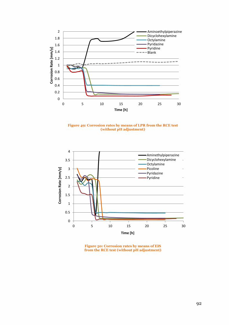
92
Figure 49: Corrosion rates by means of LPR from the RCE test (without pH adjustment)
Figure 50: Corrosion rates by means of EIS from the RCE test (without pH adjustment)
0
0.2
0.4
0.6
0.8
1
1.2
1.4
1.6
1.8
2
0 5 10 15 20 25 30
Co
rro
sio
n R
ate
[m
m/y
]
Time [h]
AminoethylpiperazineDicyclohexylamineOctylaminePyridazinePyridineBlank
0
0.5
1
1.5
2
2.5
3
3.5
4
0 5 10 15 20 25 30
Co
rro
sio
n R
ate
[m
m/y
]
Time [h]
AminethylpiperazineDicyclohexylamineOctylaminePicolinePyridazinePyridine

93
Figure 51: Potentiodynamic scans from the RCE test (without pH adjustment)
Figure 52: Corrosion rates by means of LPR from the RCE test (pH adjusted +HCl)
1E-08
0.0000001
0.000001
0.00001
0.0001
0.001
0.01
0.1
1
-1 -0.8 -0.6 -0.4 -0.2 0
Cu
rre
nt
[A]
Potential [V]
Aminomorpholine
Dicyclohexylamine
Octylamine
Pyridazine
Pyridine
Blank
0
0.2
0.4
0.6
0.8
1
1.2
1.4
1.6
1.8
2
0 5 10 15 20 25 30
Co
rro
sio
n R
ate
[m
m/y
]
Time [h]
Aminoethylpiperazine DicyclohexylamineOctylamine PyridazinePyridine Blank

94
Figure 53: Corrosion rates by means of EIS from the RCE test (pH adjusted +HCl)
Figure 54: Potentiodynamic scans from the RCE test (pH adjusted +HCl)
0
0.5
1
1.5
2
2.5
3
3.5
4
0 5 10 15 20 25 30
Co
rro
sio
n R
ate
[m
m/y
]
Time [h]
AminoethylpiperazineDicyclohexylamineOctylaminePyridazinePyridineBlankl
1E-08
0.0000001
0.000001
0.00001
0.0001
0.001
0.01
0.1
1
-1 -0.8 -0.6 -0.4 -0.2 0
Cu
rre
nt
[A]
Potential [V]
Aminoethylpiperazine
Dicyclohexylamine
Octylamine
Pyridazine
Pyridine
Blank

95
3.3.2.4.1. Conclusions from the Rotating Cylinder Test
Much information was gathered by means of the RCE tests. Excluding
aminoethylpiperazine, all the tested VCIs inhibited the corrosion in this test.
All of the other VCIs displayed some kind of alternative inhibition in addition
to the neutralisation. It can be assumed that a protective film was formed on
the surface of the corrosion sample.
Pyridazine, as one of the worst performers in the actual TOL tests, displayed
a superior performance as film forming BOL corrosion inhibitor.
3.3.2.5. Discussion and Conclusion “Low performing VCIs”
None of the tested VCIs was a satisfactory TOL corrosion inhibitor by itself.
All of the tested VCIs except of Pyridazine display a high ability to increase
the pH of an acidic solution. Due to the overall lack of satisfactory TOL
inhibition, it can also be concluded that pH neutralisation is not the
predominant inhibition mechanism in TOL corrosion inhibition by VCIs.
RCE testing showed that all of the tested VCI compounds have a good BOL
corrosion inhibition ability. Even after the solution was neutralized using
HCl, much of the inhibition ability was still remaining indicating that a large
portion of inhibition is by film forming rather than neutralisation.
In general, it can be concluded that the poor TOL inhibition in the tested
conditions is a result of the high boiling point and rather low vapour pressure
of all low performing VCIs.
3.3.2.5.1. Aminoethylpiperazine
Aminoethylpiperazine is an excellent pH neutralizer. It significantly
increased the bulk pH in all TOL tests as well as in the RCE tests. It also
displayed, in comparison to the other VCIs tested in this section, good TOL
inhibition properties. Nevertheless, the CR by means of RCE doubled to
2 mm/y after the VCI was inserted into the system. Therefore, the compound
cannot be used in the tested environments and concentrations.

96
3.3.2.5.2. Aminomorpholine
Aminomorpholine was the most expensive compound and only a very limited
amount was available for testing. Therefore, testing was stopped after it
failed to show TOL corrosion inhibition properties in the CFP.
3.3.2.5.3. Aniline
Aniline was only tested in the HCT test and therefore the conclusions are
very limited. Within the tested VCIs in the HCT, it was an average performer.
3.3.2.5.4. Dicyclohexylamine
Dicyclohexylamine isn’t volatile enough in the given conditions to have a
good effect on TOL corrosion. Despite a good inhibition in the A-HCT test, it
didn’t inhibit as well in the other TOL corrosion tests. An IE of up to 93 %
was achieved in the RCE test. Dicyclohexylamine seems to be a film forming
and neutralising amine that is not volatile enough to be part of a successful
VCI formulation that inhibits TOL corrosion.
3.3.2.5.5. Octylamine
The vapour pressure and volatility of octylamine is also not sufficient to be
effective at the TOL. The BOL inhibition, in comparison to the other VCIs
tested in this section is also underwhelming.
3.3.2.5.6. Picoline
Picoline has a negative effect on TOL corrosion. In the HCT and CFP test the
CR was increased with the injection of picoline. Therefore, it was not further
investigated on its BOL corrosion inhibition properties.

97
3.3.2.5.7. Pyridazine
Pyridazine is the only tested compound that does not have a significant
neutralisation effect on the solution. It does not inhibit in either the HCT or
A-HCT set up, but shows average TOL inhibition properties in the CFP. It
was the best performing compound (including all amines, meaning also the
high performing amines discussed later) in the RCE test in the presence of
HCl. The IE was still between 78– 84 % with HCl and up to 90 % without
HCl. It seems to be mainly a film forming inhibitor, limited to the BOL. It is
assumed that the two N atoms stick to the metal surface separating it from
the corrosion media. Further investigation might reveal possible fields of
application for a small molecular, film forming amine. Unfortunately, this is
outside the scope of this research.
3.3.2.5.8. Pyridine
The TOL inhibition of pyridine was not satisfying, but Pyridine showed
decent BOL inhibition properties without HCl in the system. An IE of 93 %
was achieved. The large part of the BOL inhibition properties was lost with
HCl being included in the testing indicating the inhibition is mainly achieved
by neutralisation.

98
3.3.3. High Performing VCIs - Results
In the following section, 8 of the generic VCI compounds will be discussed.
These 8 compounds were the compounds with the best performance in
regards of TOL corrosion inhibition. The molecular structures (displayed
using the free molecule editor software Avogadro 1.0.3) and some of the
basic properties of each molecule can be found in Table 16. The properties of
the molecules were taken from the respective MSDS sheets accessed via the
homepage of the supplier, Sigma Aldrich (MSDS 2011; MSDS 2011; MSDS
2011; MSDS 2011; MSDS 2011; MSDS 2011; MSDS 2011; MSDS 2012).
The molecular structure is displayed as grey, blue, red, and small light grey
spheres representing carbon, nitrogen, oxygen, and hydrogen, respectively.
All of the compounds are amines or involve an amino group. Amino groups
can be found either as primary, secondary, tertiary, cyclic amino group, or in
any combination. Three of the compounds contain oxygen; MDEA with two
oxygen atoms, methylmorpholine and morpholine with one oxygen atom
each. The molecular weight of all compounds lies between 73.14 and
119.16 g/mol and the boiling points are between 36 and 248 ⁰C.
The grey graph in every diagram represents the blank test, and every VCI
compound has its dedicated colour/marker combination throughout the
entire “High Performing VCI” discussion. Where necessary, some graphs
have been split up into two for clarity.

99
Table 16: Structures and properties of all high performing VCI compounds
Benzylamine Cyclohexyl-
amine Diethylamine
(DEA)
Dimethyl-ethylamine
(DMEA)
Formula C7H9N C6H13N C4H11N C4H11N
Molecular weight [g/mol]
107.15 99.17 73.14 73.14
Boiling
point [⁰C] 184-185 134 55 36-38
Vapour pressure [mm Hg]
0.662
(@ 25 ⁰C)
10
(@ 22 ⁰C)
418
(@ 20 ⁰C)
237
(@ 25 ⁰C)
Purity [%] 99 99 99 99
Molecular Structure
Methyl-
diethanol-amine (MDEA)
Methyl-morpholine
Methyl-piperazine
Morpholine
Formula C5H13NO2 C5H11NO C5H12N2 C4H9NO
Molecular Weight [g/mol]
119.16 101.15 100.16 87.12
Boiling point [⁰C]
246-248 115-116 138 126-130
Vapour pressure [mm Hg]
<0.01
(@ 20 ⁰C)
18
(@ 20 ⁰C)
7.5
(@ 20 ⁰C)
10.4
(@ 25 ⁰C)
Purity [%] 99 99 99 99
Molecular Structure

100
3.3.3.1. Horizontal Cooled Tube
In this section, the performance of the high performing VCIs is discussed. In
Figure 55 and Figure 56 the CRs by means of IC are displayed and Table 17
lists the average CRs by means of IC and WL as well as the IEs of all VCIs.
During the first 24 hours without VCI in the system, all tests averaged a CR
of around 1.50 mm/y. As soon as the VCIs were injected into the test, the CRs
drop to approximately 0.60 mm/y. The CRs kept declining until day three
(72 hours) in all tests.
Benzylamine stays constantly just below 0.40 mm/y after 72 hours until the
end of the test. A very similar behaviour can be observed for the CR of
cyclohexylamine, DEA, DMEA and methylpiperazine. They all levelled
around 0.40 mm/y until the end of the testing period.
MDEA, methylmorpholine and morpholine display a slightly different
behaviour. The CR of all three tests continues to decline slightly until the end
of the test.
Figure 57 displays the pH evolution of each test. All tested compounds alter
the pH of the bulk solution in a very similar fashion. The pH at the very
beginning of each test is 3.2. The pH of the test straight after the VCIs were
injected is in a range of 4.9 to 5.3 which is approximately 1.5 pH units higher
than the blank pH. At the end of the test, the pH ranges between 5.4 and 5.7
(blank pH 5.0). The pH in the blank test increased 1.5 pH units from day two
to day seven, whereas the VCI tests increased about 0.5 pH units during the
same time period.

101
Table 17: Corrosion rates and inhibition efficiencies by iron concentration and weight loss from the HCT test
CR [mm/y] IE [%]
IC WL IC WL
Benzylamine 0.45 0.62 37 27
Cyclohexylamine 0.44 0.65 39 24
DEA 0.42 0.58 41 32
DMEA 0.40 0.59 44 31
MDEA 0.47 0.64 35 25
Methylmorpholine 0.39 0.66 46 22
Methylpiperazine 0.40 0.65 44 24
Morpholine 0.45 0.63 37 26
Blank 0.71 0.84 - -
Figure 55: Corrosion rates from the HCT test (High performing VCIs Part 1)
0.0
0.2
0.4
0.6
0.8
1.0
1.2
1.4
1.6
1.8
2.0
0 24 48 72 96 120 144 168
Co
rro
sio
n R
ate
[m
m/y
]
Time [h]
Benzylamine CyclohexylamineDEA DMEABlank

102
Figure 56: Corrosion rates from the HCT test (High performing VCIs Part 2)
Figure 57: pH evolution from the HCT test
3.3.3.1.1. Conclusion Horizontal Cooled Tube
All VCIs discussed here have potent pH neutralisation abilities, and despite
the variety of compounds, it was not possible to really distinguish them by
0.0
0.2
0.4
0.6
0.8
1.0
1.2
1.4
1.6
1.8
2.0
0 24 48 72 96 120 144 168
Co
rro
sio
n R
ate
[m
m/y
]
Time [h]
MDEA MethylmorpholineMethylpiperazine MorpholineBlank
0
1
2
3
4
5
6
0 24 48 72 96 120 144 168
pH
Time [h]
Benzylamine CyclohexylamineDEA DMEAMDEA MethylmorpholineMethylpiperazine MorpholineBlank
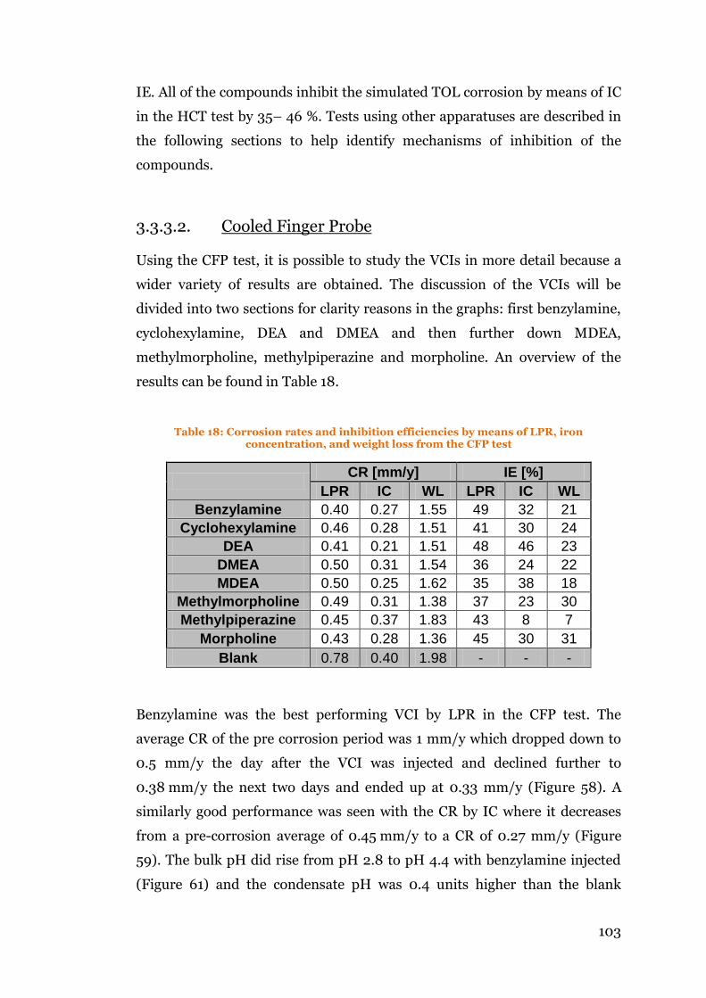
103
IE. All of the compounds inhibit the simulated TOL corrosion by means of IC
in the HCT test by 35– 46 %. Tests using other apparatuses are described in
the following sections to help identify mechanisms of inhibition of the
compounds.
3.3.3.2. Cooled Finger Probe
Using the CFP test, it is possible to study the VCIs in more detail because a
wider variety of results are obtained. The discussion of the VCIs will be
divided into two sections for clarity reasons in the graphs: first benzylamine,
cyclohexylamine, DEA and DMEA and then further down MDEA,
methylmorpholine, methylpiperazine and morpholine. An overview of the
results can be found in Table 18.
Table 18: Corrosion rates and inhibition efficiencies by means of LPR, iron
concentration, and weight loss from the CFP test
CR [mm/y] IE [%]
LPR IC WL LPR IC WL
Benzylamine 0.40 0.27 1.55 49 32 21
Cyclohexylamine 0.46 0.28 1.51 41 30 24
DEA 0.41 0.21 1.51 48 46 23
DMEA 0.50 0.31 1.54 36 24 22
MDEA 0.50 0.25 1.62 35 38 18
Methylmorpholine 0.49 0.31 1.38 37 23 30
Methylpiperazine 0.45 0.37 1.83 43 8 7
Morpholine 0.43 0.28 1.36 45 30 31
Blank 0.78 0.40 1.98 - - -
Benzylamine was the best performing VCI by LPR in the CFP test. The
average CR of the pre corrosion period was 1 mm/y which dropped down to
0.5 mm/y the day after the VCI was injected and declined further to
0.38 mm/y the next two days and ended up at 0.33 mm/y (Figure 58). A
similarly good performance was seen with the CR by IC where it decreases
from a pre-corrosion average of 0.45 mm/y to a CR of 0.27 mm/y (Figure
59). The bulk pH did rise from pH 2.8 to pH 4.4 with benzylamine injected
(Figure 61) and the condensate pH was 0.4 units higher than the blank

104
during the first 24 hours of injection, but it stayed close to the blank pH
during the rest of the test with a maximum difference of 0.2 units (Figure
62). The acetate concentration in the bulk solution slightly increases over
time from 1160 ppm on day two to 1330 ppm on day four and stayed
constant afterwards (Figure 63). By using Equation 9 it is possible to
calculate the acetic acid concentration of this test. There is 933 ppm acetic
acid in the bulk solution after 96 hours (blank test 872 ppm) and still
940 ppm of acetic acid at the very end of the test (blank 1100 ppm). So,
despite the elevated pH, the acetic acid concentration with VCI is very
comparable to the acetic acid concentration of blank test. This means the
bulk neutralisation effect is eliminated here. The acetate concentration
increases slightly because a 1000 ppm acetic acid concentration solution is
used to top up sampled liquid and accumulates acetates. Due to the VCI, the
acetate concentration in the condensed liquid decreased from 800 ppm
during the first two days down to 500 ppm over the next two days (Figure
64). Acetic acid was constantly topped up and therefore the concentration in
the condensed liquid increased back up to 650 ppm. Despite the increase, the
pH and CR was virtually unaffected which gives a positive indication for
benzylamine as a VCI.
Cyclohexylamine and DEA exhibit almost the same characteristics as
described for benzylamine. The CR by LPR of the test with cyclohexylamine
drops from 0.80 mm/y down to 0.52 mm/y and keeps decreasing to
0.41 mm/y at the end of the test (Figure 58). The CR by means of IC also
decreases over time from 0.44 mm/y during pre-corrosion down to
0.31 mm/y to a final 0.27 mm/y (Figure 59) with a very constant
condensation rate (Figure 60). The CR by LPR of DEA falls from 0.78 mm/y
the second day of pre-corrosion to 0.42 mm/y the first day of VCI in the
system and keeps decreasing to 0.35 mm/y at the end of the test. DEA
changes the CR by means of IC to the lowest CR of all tested VCIs in this
system. The CR drops from 0.38 mm/y to 0.22 mm/y down to a final
0.19 mm/y. The pH, acetate and acetic acid concentration evolution is almost
exactly the same as described before for benzylamine and will not be
described again.

105
The last VCI in this group of four is DMEA. Within this group and test,
DMEA is the least effective performing VCI, despite the comparatively low
acetic acid concentration (Figure 63). After the VCI was injected, the CR by
LPR decreased to 0.57 mm/y and kept decreasing to 0.44 mm/y at the end of
the test. The CR by means of IC levelled around 0.31 mm/y after the VCI was
injected with an average condensation rate. As mentioned, the acetic acid
concentration of the bulk solution and therefore also in the condensed liquid
was lower than the blank test. Despite the slightly less aggressive conditions
cyclohexylamine and DEA did not perform as well as benzylamine.
Figure 58: Corrosion rates by LPR from the CFP test – Part 1
0.0
0.2
0.4
0.6
0.8
1.0
1.2
1.4
1.6
1.8
2.0
0 24 48 72 96 120 144
Co
rro
sio
n R
ate
[m
m/y
]
Time [h]
Benzylamine CyclohexylamineDEA DMEABlank

106
Figure 59: Corrosion rates by iron concentration from the CFP test – Part 1
Figure 60: Condensation rates from the CFP test – Part 1
0.0
0.1
0.2
0.3
0.4
0.5
0.6
0.7
0.8
0.9
1.0
0 24 48 72 96 120 144
Co
rro
sio
n R
ate
[m
m/y
]
Time [h]
Benzylamine CyclohexylamineDEA DMEABlank
0.0
0.1
0.2
0.3
0.4
0.5
0.6
0 24 48 72 96 120 144
Co
nd
en
sati
on
Rat
e [
g/m
2/s
]
Time [h]
Benzylamine CyclohexylamineDEA DMEABlank

107
Figure 61: pH of the bulk solution from the CFP test – Part 1
Figure 62: pH of the condensed liquid from the CFP test– Part 1
0
1
2
3
4
5
6
0 24 48 72 96 120 144
pH
Time [h]
Benzylamine Cyclohexylamine
DEA DMEA
Blank
3.0
3.5
4.0
4.5
5.0
5.5
6.0
0 24 48 72 96 120 144
pH
Time [h]
Benzylamine CyclohexylamineDEA DMEABlank

108
Figure 63: Acetic acid concentration of the bulk solution from the CFP test– Part 1
Figure 64: Acetic acid concentration in the condensed liquid from the CFP test– Part 1
0
200
400
600
800
1000
1200
1400
1600
1800
2000
0 24 48 72 96 120 144
Ace
tic
acid
co
nc.
[p
pm
]
Time [h]
Benzylamine CyclohexylamineDEA DMEABlank
0
200
400
600
800
1000
1200
1400
1600
1800
2000
0 24 48 72 96 120 144
Ace
tic
acid
co
nc.
[p
pm
]
Time [h]
Benzylamine CyclohexylamineDEA DMEABlank

109
The second set of four VCIs includes MDEA, methylmorpholine,
methylpiperazine and morpholine. The evolution of the CR by means of LPR
for all four VCIs is nearly identical. During the pre-corrosion the CR is
around 1.00 mm/y and it falls to 0.6 mm/y, 0.55 mm/y, 0.47 mm/y and
0.43 mm/y for MDEA, methylmorpholine, methylpiperazine and
morpholine, respectively. The CR for all four VCIs falls further over the next
three days between 0.43 mm/y and 0.50 mm/y (Figure 65).
The CRs by means of IC are more separated on first appearance (Figure 66).
Methylpiperazine stands out with a higher CR than the other VCIs. By
comparing the condensation rates of the VCIs, it becomes clear that the
condensation rate of methylpiperazine is higher than all others (Figure 67).
Also seen in all other tests before, the CR is affected very much by the
condensation rate. Despite the higher condensation rate, methylpiperazine
still keeps the CR below the blank CR. A similar effect can be seen by
methylmorpholine where the condensation rate briefly increases after 96 and
120 hours. With the increase in condensation rate, the CR increases, too. The
CR by IC for MDEA, methylmorpholine and morpholine decreases from
around 0.40 mm/y pre corrosion to 0.27 mm/y corrosion with VCI. At the
end of the test, all three show a CR around 0.27 mm/y (Figure 66). The
acetate concentrations are higher than the blank and therefore, the acetic
acid concentrations are again (as with the first set of four VCIs) very
comparable with the blank test. The pH of the bulk solution is between 4.3
and 4.6 the day of VCI injection and falls to between pH 4.1 and 4.4 until the
end of the test (Figure 68). The pH of all four VCIs in the condensed liquid
the day after injection is also very similar and lies between pH 5.3 and 5.4. It
falls to pH 5.0 at the end of the test with MDEA, methylmorpholine and
morpholine (Figure 69). The pH of methylpiperazine falls to pH 4.77 a day
before the end and stays constant on the last day. This might be in
correlation with the increase of condensation rate during the last two days.
The average CRs and IEs in Table 18 on page 103 also indicates how similar
the tested VCIs in this section are especially in regards of the CR and IE by
means of LPR.

110
Figure 65: Corrosion rates by LPR from the CFP test – Part 2
Figure 66: Corrosion rates by iron concentration from the CFP test – Part 2
0.0
0.2
0.4
0.6
0.8
1.0
1.2
1.4
1.6
1.8
2.0
0 24 48 72 96 120 144
Co
rro
sio
n R
ate
[m
m/y
]
Time [h]
MDEA MethylmorpholineMethylpiperazine MorpholineBlank
0.0
0.2
0.4
0.6
0.8
1.0
1.2
1.4
1.6
0 24 48 72 96 120 144
Co
rro
sio
n R
ate
[m
m/y
]
Time [h]
MDEA Methylmorpholine
Methylpiperazine Morpholine
Blank

111
Figure 67: Condensation rates from the CFP test – Part 2
Figure 68: pH of the bulk solution from the CFP test – Part 2
0.0
0.1
0.2
0.3
0.4
0.5
0.6
0 24 48 72 96 120 144
Co
nd
en
sati
on
Rat
e [
g/m
2/s
]
Time [h]
MDEA Methylmorpholine
Methylpiperazine Morpholine
Blank
0
1
2
3
4
5
6
0 24 48 72 96 120 144
pH
Time [h]
MDEA Methylmorpholine
Methylpiperazine Morpholine
Blank

112
Figure 69: pH of the condensed liquid from the CFP test – Part 2
Figure 70: Acetic acid concentration of the bulk solution from the CFP test – Part 2
3.0
3.5
4.0
4.5
5.0
5.5
6.0
0 24 48 72 96 120 144
pH
Time [h]
MDEA MethylmorpholineMethylpiperazine MorpholineBlank
0
200
400
600
800
1000
1200
1400
1600
1800
2000
0 24 48 72 96 120 144
Ace
tic
acid
co
nc.
[p
pm
]
Time [h]
MDEA Methylmorpholine
Methylpiperazine Morpholine
Blank

113
Figure 71: Acetic acid concentration in the condensed liquid from the CFP test– Part 2
3.3.3.2.1. Conclusion Cooled Finger Probe
All of the “high performing” compounds tested in the CFP display very
similar properties to each other. For example, the pH of the bulk solution of
each of the tested compounds the day of injection is between pH 4.3 and pH
4.6 and at the end of the test, the pH is between pH 4.1 and pH 4.5. The pH
of the condensed liquid (except for DMEA) also lies in a very tight range,
between pH 4.8 and pH 5.1 at the end of the test. More importantly, the
evolution of the CRs and the resulting IEs are very similar, too. It can be
concluded that all of the tested VCIs in this section work well in inhibiting
TOL corrosion in the given conditions provided by the CFP test.
3.3.3.3. Altered Horizontal Cooled Tube
In this section, the performance of the “high performing VCIs” in the A-HCT
will be discussed. The average CRs and IEs are listed in Table 19 and it is
obvious that the performance of the VCIs show more variation than with the
CFP test in the section before. Therefore, the results of the “high performing
VCIs” are displayed in one graph for each parameter: CRs, condensation
0
200
400
600
800
1000
1200
1400
1600
1800
2000
0 24 48 72 96 120 144
Ace
tic
acid
co
nc.
[p
pm
]
Time [h]
MDEA Methylmorpholine
Methylpiperazine Morpholine
Blank

114
rates, bulk pH, and condensed pH (Figure 72, Figure 73, Figure 74, and
Figure 75).
The bulk pH is an important indication in these results. It should start low
which would ensure that the VCI and the bulk solution have good separation.
The tests discussed in this section have a low starting pH except for
methylmorpholine and DEA. Both of those VCI tests start up with a bulk pH
of over pH 4 and therefore the results need to be evaluated with care and it
might be necessary to exclude the results from the following discussions
(Figure 74).
The average CR of benzylamine by means of IC and WL is 1.14 mm/y and
1.12 mm/y, respectively resulting in an IE of 29 % and 14 %. The CR starts at
1.30 mm/y and declines on day two to 0.80 mm/y with the condensation rate
staying constant around 0.44 g/m2/s. On day three, the CR increases back up
to 1.25 mm/y and then just increases slightly to 1.32 mm/y on day four as the
condensation rate also increases up to 0.60 g/m2/s on day three and four.
The condensed pH stays around pH 6.0 throughout the test. The high
condensed pH is very similar to the blank version and is mainly due to the
reasonably high corrosion rate. Benzylamine is not a suitable VCI in this test
set up.
Cyclohexylamine displays just slightly better inhibition than benzylamine.
The CR declines from 1.35 mm/y on day one to 1.01 mm/y on day three and
increases again to 1.25 mm/y during the last 24 hours (Figure 72). A slightly
increase in condensation rate is also observed in this test from 0.33 g/m2/s
to 0.49 g/m2/s over the four days of testing. The effect on the pH of the
condensed liquid is also limited, and the pH stays constantly around 6.0.
As mentioned in the beginning of this section, the bulk pH of DEA starts off
high. Additionally, the condensation rate is comparatively low (0.32 g/m2/s-
0.43 g/m2/s) which results inevitably in a low CR. The same can be said
about methylmorpholine. It has a high pH in the bulk solution at the
beginning and the condensation rate is even lower. Both results will not be in
the assessment of the performance of these VCIs.

115
DMEA shows a very good IE by means of IC and WL of about 64 % and 58 %,
respectively (Table 19). The CR starts at 0.72 mm/y and decreases to a final
0.49 mm/y on day four. The condensation rate starts low around
0.32 g/m2/s but doubles over the next days to 0.65 g/m2/s but the CR stays
low. The pH in the bulk solution starts at a very low pH of 3.4 and increases
to pH 5.6 over the test duration. The huge increase indicates that DMEA has
comparatively high volatility. The pH of the condensed liquid starts slightly
lower than the pH of the other VCIs at pH 5.7 and decreases to pH 4.8 at the
end of the test. All results of this test together indicate very good inhibition
behaviour of DMEA.
MDEA also displays very good IEs by means of IC and WL of 56 % and 60 %,
respectively. With a rising condensation rate and a consistently low bulk pH,
the CR decreases from 1.1 mm/y in the beginning of the test to 0.39 mm/y
after three days. As the condensation rate keeps increasing, the CR also
increases to a final of 0.70 mm/y.
Methylpiperazine has the highest IE by means of IC in the A-HCT test of all
tested VCIs with in IE of 65 % (excluding DEA and methylmorpholine for the
high pH and low condensation rates). The CR by IC declines during the test
from 0.78 mm/y to 0.34 mm/y by the end. The condensation rate increases
from 0.33 g/m2/s to 0.50 g/m2/s during the test and is comparatively low
after four days. The pH of the bulk solution increases from pH 3.9 to pH 5.3
and the pH in the condensed liquid decrease from pH 6.2 to pH 5.3.
The pH of the bulk solution and condensed liquid of morpholine is
essentially the same as the just described methylpiperazine. The
condensation rate in the case of morpholine was higher than in any of the
other VCIs tests. An IE of 49 % and 42 % for IC and WL, respectively, is a
very good result given the slightly harsher circumstances. The CR after day
two is constant around 0.70 mm/y.

116
Table 19: Average corrosion rates and inhibition efficiencies by iron concentration and weight loss from the A-HCT test
CR [mm/y] IE [%]
IC WL IC WL
Benzylamine 1.14 1.12 29 14
Cyclohexylamine 1.16 1.00 28 23
DEA 0.47 0.54 71 58
DMEA 0.58 0.56 64 58
MDEA 0.71 0.53 56 60
Methylmorpholine 0.43 0.59 73 55
Methylpiperazine 0.56 0.72 65 45
Morpholine 0.82 0.76 49 42
Blank 1.61 1.31 - -
Figure 72: Corrosion rate by iron concentration from the A-HCT test
0.0
0.5
1.0
1.5
2.0
2.5
0 24 48 72 96
Co
rro
sio
n R
ate
[m
m/y
]
Time [h]
Benzylamine CyclohexylamineDEA DMEAMDEA MethylmorpholineMethylpiperazine MorpholineBlank

117
Figure 73: Condensation rate from the A-HCT test
Figure 74: Bulk pH from the A-HCT test
0
0.1
0.2
0.3
0.4
0.5
0.6
0.7
0.8
0.9
1
0 24 48 72 96
Co
nd
en
sati
on
Rat
e [
g/m
2/s
]
Time [h]
Benzylamine CyclohexylamineDEA DMEAMDEA MethylmorpholineMethylpiperazine MorpholineBlank
0
1
2
3
4
5
6
7
0 24 48 72 96
pH
Time [h]
Benzylamine CyclohexylamineDEA DMEAMDEA' MethylmorpholineMethylpiperazine MorpholineBlank

118
Figure 75: Condensed liquid pH from the A-HCT test
3.3.3.3.1. Conclusions Altered Horizontal Cooled Tube
The A-HCT test must be performed with utmost care to produce reliable
results. Nevertheless, it seems to be a great test for research purposes under
high pressure due to unique set of data it produces.
All of the tested high performing VCIs have a positive impact on the CR in
the A-HCT test.
3.3.3.4. Rotating Cylinder Electrode
The last experiments to be discussed are the RCE tests of the high
performing VCIs. In Figure 76 and Figure 77 the CR is displayed calculated
by means of LPR and EIS, respectively. The CRs at the beginning of the test
(approximately 5 hours) are the blank CRs of the respective tests; around
1.00 mm/y for LPR and 2.5 mm/y for EIS measurements. While tests were
running, the VCI was injected into the system to alter the CR.
The characteristic of the CR evolution was the same for every compound; the
CR dropped drastically to a lower value and remained there until the end of
0
1
2
3
4
5
6
7
0 24 48 72 96
pH
Time [h]
Benzylamine CyclohexylamineDEA DMEAMDEA MethylmorpholineMethylpiperazine MorpholineBlank

119
the test. The CR over time curves calculated from the LPR tests are shown in
Figure 76 and for EIS they are displayed in Figure 77. Most of the resulting
CRs at the end of the tests are within a narrow window. The CR calculated by
LPR for the tests with Cyclohexylamine, DEA, DMEA, MDEA,
methylmorpholine, and morpholine all drop abruptly to a lower CR as soon
the VCI was injected and stabilizes between 0.40 mm/y and 0.75 mm/y. A
very similar picture can be seen in the evolution in the CR by calculated by
EIS where the resulting CRs dropped down between 0.59 mm/y and
0.86 mm/y. The IEs of the mentioned generic VCIs are in the range of 34 % -
58 % and 66 % - 75 % by LPR and EIS, respectively (Table 20).
The potentiodynamic scans are displayed in Figure 78. None of the VCIs
significantly affects the potential or the anodic side of the curve in any way.
The maximum difference in corrosion potential from the blank is less than
25 mV. All of the VCIs slightly lower the cathodic current.
To investigate the mechanism of inhibition of the VCIs, a second test was run
where the effect of the VCI on the pH was eliminated by adding an
appropriate amount of HCl to adjust the pH back to pH 3.15. The CR graphs
are shown in Figure 79 and Figure 80 and the IEs are listed in the second
column of Table 20. The CRs calculated by LPR indicate a large drop in
inhibition as the HCl is added. In Figure 79 it can be seen that the curves are
spread out more than without HCl and the IEs are much lower between 0% -
32 %. The same tests investigated by EIS indicate a better inhibition ability of
the compounds. The resulting CRs are altogether higher than without HCl
added into the system, but with IEs between 34 % - 66% much more efficient
than calculated by LPR. In this case, the EIS results are more trustworthy. As
described under Rotating Cylinder Electrode (RCE) Test in section 3.2.5,
LPR cannot distinguish between solution resistance (RS) and charge transfer
resistance (RCT). In the experiments involving addition of VCI and HCl the
charge transfer resistance increases due to inhibition but the effect is
diminished in the LPR measurements by a smaller solution resistance due to
the addition of VCI and more importantly HCl and NaOH to adjust the pH.
The amines have a higher film forming ability as seen with the LPR tests.

120
The two remaining VCI compounds are benzylamine and methylpiperazine.
Benzylamine displays very good inhibition as calculated by both LPR and EIS
with a final CR of 0.12 mm/y and 0.13 mm/y and an IE of 88 % and 97 %,
respectively. Methylpiperazine actually increases the CR significantly in all
tests without HCl in the cell and therefore it was not possible to calculate an
IE for this compound. Almost surprisingly, methylpiperazine does have a
positive effect on the CR in the tests with HCl included. It shows a calculated
IE of 44 % and 72 % by LPR and EIS, respectively. The compound decreases
the CR significantly straight after it was injected into the system, but the CR
increases over time as calculated by both, LPR and EIS.
Benzylamine on the other hand still displays a very good IE with HCl in the
system. The IE calculated by EIS is 79 % and therefore this is the most
effective of the high performing VCIs in the presence of HCl.
In Figure 81, the potentiodynamic scans are displayed of the tests with HCl.
None of the curves are affected in a major fashion by any of the VCIs
including HCl. The corrosion potential is shifted not more than 40 mV, this
to a more cathodic value, though. Nevertheless, neither the cathodic nor the
anodic corrosion current is significantly affected and stays very close to the
blank curve.
Table 20: Inhibition efficiencies by LPR and EIS from the RCE test set up without and with pH adjustment (+HCl)
[%] IE by LPR (Figure 76)
IE by EIS (Figure 77)
IE by LPR + HCl (Figure 79)
IE by EIS + HCl (Figure 80)
Benzylamine 88 97 59 79
Cyclohexyl-amine
42 70 0 34
DEA 40 66 10 39
DMEA 34 67 19 55
MDEA 51 75 33 66
Methyl-morpholine
47 72 23 61
Methyl-piperazine
- - 44 72
Morpholine 58 - 32 65

121
Figure 76: Corrosion rate by LPR from the RCE test (without pH adjustment)
Figure 77: Corrosion rate by EIS from the RCE test (without pH adjustment)
0
0.5
1
1.5
2
2.5
0 5 10 15 20 25 30
Co
rro
sio
n R
ate
[m
m/y
]
Time [h]
Benzylamine CyclohexylamineDEA DMEAMDEA MethylmorpholineMethylpiperazine MorpholineBlank
0
0.5
1
1.5
2
2.5
3
3.5
4
0 5 10 15 20 25 30
Co
rro
sio
n R
ate
[m
m/y
]
Time [h]
BenzylamineCyclohexylamineDEADMEAMDEAMethylmorpholineMethylpiperazine

122
Figure 78: Potentiodynamic scans from the RCE test (without pH adjustment)
Figure 79: Corrosion rate by LPR from the RCE test (pH adjusted +HCl)
1.00E-09
1.00E-08
1.00E-07
1.00E-06
1.00E-05
1.00E-04
1.00E-03
1.00E-02
1.00E-01
1.00E+00
-1 -0.8 -0.6 -0.4 -0.2 0
Cu
rre
nt
[A]
Potential [V]
CyclohexylamineDEADMEAMDEAMethylmorpholineBlank
0
0.2
0.4
0.6
0.8
1
1.2
1.4
1.6
1.8
2
0 6 12 18 24
Co
rro
sio
n R
ate
[m
m/y
]
Time [h]
Benzylamine CyclohexylamineDEA DMEAMDEA MethylmorpholineMethylpiperazine MorpholineBlank

123
Figure 80: Corrosion rate by EIS from the RCE test (pH adjusted +HCl)
Figure 81: Potentiodynamic scans from the RCE test (pH adjusted +HCl)
0
0.5
1
1.5
2
2.5
3
3.5
4
0 5 10 15 20 25 30
Co
rro
sio
n r
ate
[m
m/y
]
Time [h]
Benzylamine CyclohexylamineDEA DMEAMDEA MethylmorpholineMethylpiperazine MorpholineBlank
1E-09
1E-08
0.0000001
0.000001
0.00001
0.0001
0.001
0.01
0.1
1
-1 -0.8 -0.6 -0.4 -0.2 0
Cu
rre
nt
[A]
Potential [V]
BenzylamineCyclohexylamineDEADMEAMDEAMethylmorpholineMorpholineBlank

124
3.3.3.4.1. Conclusions Rotating Cylinder Electrode
The high performing VCIs show a very positive behaviour in the RCE test. All
of the tested VCIs show an IE of over 66 % calculated by EIS. The addition of
HCl distinguishes the different modes of inhibition of the different VCIs. IEs
with HCl range from 34 % - 79 % calculated by EIS. In general, the low
performing VCIs are better BOL inhibitors than the high performing VCIs.
EIS investigation is much better suited to the conditions tested in this
investigation. 0.1 % NaCl solution is not conductive enough to gain
trustworthy results by means of LPR. Especially in TOL corrosion
investigations where condensed waters are replicated or directly measured,
LPR tests seem to be misleading and inhibition properties of VCIs can be
underestimated.
On the positive side, LPR overestimates the CR which is the more
conservative outcome and therefore preferred by pipeline operators.
Unfortunately, a VCI compound which actually works to protect against TOL
corrosion, or even a fully formulated VCI, may be rejected as an option to
inhibit the TOL because of a misleading measurement in the laboratory or in
the field since many of the monitoring techniques utilise LPR to monitor the
CR in the field.
3.3.3.5. Discussion and Conclusions “High Performing VCIs”
In this section, all the results for the individual VCIs will be discussed
including the results of the individual test methods. The EIS results are used
to draw conclusions for the RCE test.
3.3.3.5.1. Benzylamine
Benzylamine was an overall well performing compound despite its high
boiling point and low vapour pressure. TOL corrosion was successfully
inhibited in the HCT and CFP with a better performance in the LPR test than
the WL or IC measurements. The performance in the A-HCT test was not
very good.

125
The RCE tests with and without HCl were the best of the high performing
VCIs with an IE of 97 % and 79 % with and without HCl as calculated by EIS,
respectively. The very high IE with HCl in the system indicates that
Benzylamine is forming a stable film on the steel surface that separates the
steel form the corrosive media around.
Due to the low vapour pressure, high boiling point and the results gained in
the TOL corrosion test set-ups, it is concluded that the inhibition by
benzylamine is mainly by neutralizing the bulk solution and not by forming a
film on the TOL. Nevertheless, RCE tests at the BOL indicate that
benzylamine is also form a film on the surface.
3.3.3.5.2. Cyclohexylamine
Cyclohexylamine was consistently an average performing VCI. The
performance was average in the HCT and CFP but not good in the A-HCT.
Due to these results it can be concluded that the boiling point and vapour
pressure are still not favourable enough to make cyclohexylamine a very
good TOL VCI compound. Most of its inhibition results from the
neutralisation of the bulk solution and in the given conditions the volatility is
too low so not enough of the VCI compound reaches the TOL.
Cyclohexylamine displayed an IE of 70 % in the RCE test. As soon HCl was
added IE dropped to 34 %. This indicates a poor film forming capability of
cyclohexylamine.
3.3.3.5.3. Diethylamine (DEA)
DEA was one of the best performing VCIs across all TOL corrosion test
methods. It has a strong ability to neutralize the bulk solution. It displayed
the best IE by WL in the HCT test. It also decreased the CR by means of IC in
the CFP to the lowest value resulting in the highest IE by IC of 46 % (the next
best IE by IC is 32 %). The performance in the A-HCT is also very good. Due
to the high starting pH and therefore bulk neutralisation in the A-HCT test it
can’t be significantly relied on, but the performance in the A-HCT goes along

126
with the overall performance of DEA. DEA has a low boiling point of 55 ⁰C
and a very high vapour pressure of 418 mmHg (at 20 ⁰C). This seems to
confirm the necessity of a low boiling point a high vapour pressure as
characteristic for a successful VCI for TOL corrosion inhibition. The boiling
point of DEA was in between the bulk solution temperature of the TOL tests
(80 and 91 ⁰C) and the test sample temperatures (below 55 ⁰C). The boiling
point was just right for the compound to evaporate from the bulk solution
and condense at the TOL and inhibit corrosion. This could explain the rather
good TOL inhibition properties despite the rather poor BOL inhibition
properties tested in the RCE. DEA was just right for the conditions in the
TOL corrosion tests.
The performance in the RCE test, with an IE of 66 % without and 39 % with
the addition of HCl was lower than average. A large part of the inhibition
seems to result from film forming.
The results indicate that DEA neutralizes the bulk solution and it seems to be
volatile enough to reach the TOL. It then can form a film and neutralize the
condensing liquid right at the TOL.
3.3.3.5.4. Dimethylethylamine (DMEA)
DMEA has excellent neutralisation properties and therefore shows a good
inhibition in the HCT test and also the A-HCT test. The performance in the
CFP was lower than average.
The IE in the RCE test without HCl was with 67 % also lower than average.
The IE with HCl was with 55 % also on the lower end of the VCIs but it also
shows that a huge part of the inhibition seems to be a result of film forming.
Additionally to the neutralisation of the bulk solution, DMEA has a very low
boiling point and high vapour pressure and is therefore volatile. Similarly to
DEA, the BOL inhibition is low compared to the other tested VCIs but the
TOL inhibition is rather good. It can again be concluded that the boiling
point of DMEA is located just right for this test where due to the high
temperature the VCI evaporates from the bulk solution and co-condenses at

127
the TOL due to the lower temperature. DMEA seems to neutralise the
condensed liquid and forms a film on the steel surface.
3.3.3.5.5. Methyldiethanolamine (MDEA)
Within the “high performing VCIs”, MDEA has the weakest pH
neutralisation ability which can be seen in the bulk pH of the HCT and CFP.
The IE by means of IC was the lowest in the HCT test and also the lowest by
means of LPR in the CFP. The IE by means of IC in the A-HCT is
comparatively low but shows a certain inhibition effect. Nevertheless, the
compound shows a good inhibition in the RCE test set up and maintains
most of the IE in the tests including HCl with 75 % and 66 %, respectively.
Due to its high boiling point it is not very volatile, but MDEA seems to be
protective directly at the TOL as seen in the A-HCT test. Much of the
performance comes from its film forming abilities.
3.3.3.5.6. Methylmorpholine
Methylmorpholine seems to work well in the HCT and A-HCT with 46 % and
73 % IE by IC, respectively. Both values are the highest in the respective test
set up. In the CFP test, the performance was average except for the WL data
with an IE of 30 % which is just 1 % short of morpholine as the best
performing VCI. The LPR performance was relatively good with an IE of
72 % without HCl and 61 % with HCl.
Methylmorpholine shows potential in the pressurised test set ups. It shows
volatility but most of the performance comes from neutralisation of the bulk
solution. In the RCE test it shows a pronounced film forming ability.
3.3.3.5.7. Methylpiperazine
Methylpiperazine is one of the better performing VCIs in all tests. In the CFP
though, it reaches an IE of 43 % by means of LPR and only 8 % and 7 % of IE
by means of IC and WL, respectively, both the lowest measured values. A

128
comparatively high condensation rate is responsible for the high CR rates by
means of IC and WL. Taking all test results into account, methylpiperazine
performed well as a VCI.
Methylpiperazine seems to increase the CR in the given conditions and
concentration in the RCE test without HCL. When HCl was added into the
test as a neutraliser, the IE was comparatively good at 72 %.
Due to the good inhibition of methylpiperazine, the increasing CR at the BOL
inhibition should be investigated further. Experiments at a lower
concentration should be valuable.
Methylpiperazine is a volatile compound with good film forming,
neutralizing, and inhibiting properties.
3.3.3.5.8. Morpholine
Morpholine is the smallest cyclic compound in the high performing section.
It is an average performing compound with solid IEs throughout the tests. In
the A-HCT test it was challenged with the highest condensation rates which
probably resulted in a lower IE.
In the RCE test with HCl morpholine showed a residual IE of 65 % indicating
a high possibility of film forming.
The volatility of morpholine is sufficient to reach the TOL and inhibit there
directly by neutralisation and film formation. As with all other high
performing VCIs, morpholine also neutralises the bulk solution.

129
3.3.4. Conclusion Generic VCI Compounds
Several generic VCI compounds were tested in a variety of test set ups.
Unfortunately, the “silver bullet” against TOL corrosion was not within the
tested compounds.
Nevertheless, some important data about the chemical compounds was
gathered during the experiments. The conclusions of the separate
compounds have been presented after the tests under “Low performing
VCIs” and “High performing VCIs”.
In general, it seems that the boiling point is one very important property of a
successful VCI compound. Most of the low performing VCI compounds have
high boiling points. The lowest boiling point was 115 ⁰C for pyridine, with all
other low performing compounds having a boiling point of 145 ⁰C and
higher, up to 256 ⁰C. In the high performing VCIs, the compounds with the
highest boiling points were MDEA, benzylamine and then cyclohexylamine
where two of the three performed poorly in the A-HCT test where volatility is
a key property. DEA and DMEA, the two compounds with the lowest boiling
point (and highest vapour pressure) were performing well in the TOL tests
despite both were exhibiting a “lower than average” IE in the RCE tests. In
other words, this means that the n actual inhibition ability of the compounds
is low compared to the other contestants but due to the “right” boiling point
the compounds are able to evaporate from the bulk solution and re-condense
at the TOL at a higher rate and therefore perform the inhibition to a more
satisfactory grade. These results highlight the importance of choosing the
right compound for the right circumstance.
The chemical structure is another important property. Four out of six low
performing cyclic amines contain a benzene ring where just one of the high
performing VCIs has a benzene ring, benzylamine. The benzene ring is not
responsible for the high boiling point, but seems to be disadvantageous for
TOL corrosion inhibition.

130
Overall, to be able to inhibit TOL corrosion directly, the boiling point must
be low, the volatility high, and the molecular weight low. These necessary
properties are usually not found in a film forming compound since these are
traditionally long chained polar molecules. Therefore, all of the tested and
more successful TOL inhibitors have stronger neutralisation ability than film
forming ability. Nevertheless, most compounds also tend to form a film on
the surface which does inhibit TOL corrosion to some extent.
A very positive finding was made on BOL corrosion inhibition with
pyridazine. Despite the very small size of the molecule a very strong
inhibition was revealed in the RCE test set up. More importantly, the
inhibition effect is solely due to film forming effects since pyridazine had
virtually no effect on the pH and in the RCE test that did include HCl most of
the inhibition was still observed. Pyridazine reached an IE of 90 % in the
RCE tests with 84 % left with HCl in the system. Compared to many other
BOL inhibition compounds 90 % IE at a concentration of 1000 ppm is
relatively poor performance. Nevertheless, further research might reveal that
pyridazine might be a good candidate for niche applications like under
deposit corrosion or it might be useful as an additional compound in a
formulated BOL corrosion inhibitor.

131
4. Top-of-the-Line Corrosion Test Set-ups
4.1. Introduction
There are numerous TOL corrosion test methods in use. Many research
groups and virtually every company which produce and sells VCIs have their
own method of TOL corrosion testing and VCI testing (Pots and Hendriksen
2000; Gough et al. 2009; Singer et al. 2009; Gunaltun et al. 2010;
Kashkovskiy and Kuznnetsov 2012; Oehler et al. 2012). All of the methods
produce different results and are difficult to compare.
Experience with the different set-ups was gained during the research.
Advantages and disadvantages of the test methods will be assessed and
suggestions for improvements will be made.
An improved set-up will be proposed to be used for future TOL corrosion and
VCI research at Curtin University. If accepted by others, it could also cater as
a standardized method for VCI research to be able to independently test and
compare the efficiency of VCIs in different laboratories.

132
4.2. Discussion
The experiments discussed in the previous chapters are used and examined
from the perspective of the test method rather than the angle of corrosion.
The HCT (introduced in section 2.2), A-HCT (introduced in section 0), CFP
(introduced in section 3.2.3) as TOL corrosion test methods and the RCE test
(introduced in section 3.2.5) as a BOL or condensed liquid test method are
discussed in this section.
All of the TOL corrosion tests used in this research are static systems, which
do not take any gas flow into consideration. Any dynamic system is more
complicated and consists of more moving parts increasing the initial and
running costs of the system. Nevertheless, the results show that the HCT set-
up is generally suitable for performing TOL corrosion research. Indeed, all of
the test methods are applicable to perform VCI research, each with its own
advantages and disadvantages.
4.2.1. Horizontal Cooled Tube (HCT) Test
The HCT test was already largely improved from its original U-tube design,
in which the sample was hanging in a U-shape and all the condensate
collected at the lowest point as explained in section 2.3.1 and displayed in
Figure 6 (John et al. 2009).
One problem is the test sample preparation by sandblasting. An effort was
made to keep a constant ratio of fresh to used garnet in the sandblaster to
maintain the same sample surface for each test. As the garnet is used over
time the grains become smaller and rough edges are smoothened and
therefore the surface roughness decreases. A smaller surface area is the
result of the reduced surface roughness which decreases the condensation
rate which again reduces corrosion. Hence, the consistency of the garnet
can’t be guaranteed as it can be by using a new set of grinding paper unless
fresh garnet is used at all times. Maintaining fresh garnet at all times would
be possible, but was not achievable for the amount of testing during the

133
research (over 110 tests with a cooled tube set-up) and the very old and basic
sandblaster used.
The major disadvantage for the test set-up would be the fact that the
condensed liquid drops into the bulk solution, which elevates the pH and
therefore decreases the availability of free acetic acid. As can be seen in the
CR calculated by means of AAS for the blank sample, the CR drops
significantly after two days, most likely due to the rising pH (Figure 82). The
composition of condensed liquid and bulk cannot be studied separately for
the same reasons.
The biggest advantage of the system clearly is its ability to perform high
pressure and high temperature testing. Investigations can be performed at
exactly the same conditions as found or expected in the field. By adjusting
the temperature of the cooling fluid (therefore the sample temperature) and
the autoclave temperature, it is possible to achieve a vast variety of
condensation rates. In fact it even allows the adjustment of the condensation
rate throughout the experiment. Another positive feature is that the pressure
reactor and control unit are basically an “off the shelf” item with just minor
modifications. The parts for the HCT could be ordered, built, and used all
over the world with minimal effort or modifications. The test sample is also
commercially available as a ¼ inch carbon steel tube, which could be
exchanged for any available ¼ inch tube material.
In the case of VCI investigation, the high pressure pipette allows for pre-
corrosion of the test sample before an inhibiting chemical is injected into the
system. It would also be possible to replenish the bulk solution completely,
keeping the system under pressure.

134
Figure 82: CR calculated by IC and pH in the HCT test
4.2.2. Altered Horizontal Cooled Tube (A-HCT) Test
The difference between A-HCT and HCT are the two added stainless steel
cups; one to collect the condensed liquid and the second to hold the VCI and
separate it from the bulk solution. The test was designed to be used with
VCIs, especially to investigate the effect of VCIs directly to the TOL,
eliminating neutralisation effects in the bulk solution.
The “weak point” of the set-up is actually the lower beaker that holds the VCI
solution. The vessel is pressurized and de-pressured to remove oxygen out of
the system. The pressurizing is performed with the sparge tube through the
bulk solution of the autoclave. This procedure often splashes up the bulk
solution which sometimes floods the content (VCI solution) of the lower
beaker in to the bulk solution. The VCI then increases the pH of the bulk
solution, which in turn makes the second cup redundant and even worse, this
happens in an uncontrolled fashion.
Slight modifications on the equipment, like a conical cup and a gas disperser
to avoid the extensive splashing and flooding could substantially increase the
value of the test set-up.
0.0
1.0
2.0
3.0
4.0
5.0
6.0
0.0
0.2
0.4
0.6
0.8
1.0
1.2
1.4
1.6
1.8
0 24 48 72 96 120 144 168
pH
Co
rro
sio
n R
ate
[m
m/y
]
Time [h]
Blank CR-IC Blank pH

135
Nevertheless, in the blank test, it can be seen that the condensed liquid
doesn’t alter the pH of the bulk solution due to the collecting beaker.
Therefore the CR stays high (Figure 83). Separating the condensed liquid
and bulk solution has been proven to be important for a robust TOL
corrosion test method.
Figure 83: Corrosion rate by IC, condensation rate, condensed pH and bulk pH of the blank test from the A-HCT set-up
4.2.3. Cooled Finger Probe (CFP) Test
The CFP test operates under ambient pressure and needs CO2 sparging
continuously to maintain an oxygen-free environment, increasing the
running costs of a test. Nevertheless, the CFP test is very well suited for VCI
testing and evaluation. The collection cup and LPR probe of the test make it
possible to run in-situ electrochemical tests of the condensed liquid, adding
another source of information beside WL and IC. The beaker also makes it
possible to determine the exact condensation rate of the preceding 24 hour
period, identifying irregularities in the test.
0
1
2
3
4
5
6
7
8
0 24 48 72 96Time [h]
Blank CR-IC [mm/y] Condensation Rate [g/m2/s]
Blank pH cond. Blank pH bulk
136
The CFP is limited in its application for TOL corrosion research due to the
inability to operate at higher pressures, and therefore it is limited to bulk
solution temperatures of less than 100 ⁰C.
An improvement to the set up would be the exchange of LPR tests to EIS
tests. As seen in the RCE test in the previous chapter, LPR is not well suited
in condensed water conditions with low conductivity. Therefore, EIS would
improve the significance of the results gained by electrochemical testing of
the condensed liquid.
4.2.4. Rotating Cylinder Electrode (RCE) Test
RCE tests are a very useful research tool for most kinds of corrosion,
including TOL corrosion. It is possible to replicate the condensed liquid and
investigate its corrosivity in a simple set-up. It is also possible to investigate
the performance of VCIs as demonstrated in the previous chapter.
In tests with a relatively high solution resistance or in instances where the
conductivity of the solution might be changed by the addition of inhibitor or
any other substance, EIS should be chosen to investigate the corrosion
processes. In the VCI investigation discussed in the previous chapter, the
solution resistance (RS) decreased with the addition of VCI and HCl (Figure
84 from RS1 to RS2). Due to the inhibition effect of the VCI the polarisation
resistance (RCT) increased (Figure 84 from RCT1 to RCT2). The inhibition was
not very strong, but existed and was recorded by EIS. LPR on the other hand
did not record any changes in CR and the inhibitor appeared not to have any
effect on the system whatsoever.
Therefore, for future TOL corrosion research, EIS should be used for both,
RCE and CFP testing. It reinforces the confidence in the results and increases
the amount of valuable information gathered.

137
Figure 84: Nyquist plot of EIS measurement with and without VCI
-50
-45
-40
-35
-30
-25
-20
-15
-10
-5
0
0.00 20.00 40.00 60.00 80.00 100.00 120.00
Z"
Z'
RS2
RS1 RCT1
RCT2
RLPR

138
4.3. Conclusion Improved TOL Corrosion
Research Test Method
Combining all the experience gained by handling different TOL corrosion
test methods, an improved set-up for TOL corrosion research and VCI
evaluation can be proposed based on the HCT test.
The major problem with the HCT test was that the condensed liquid drips
into the bulk solution, increasing the pH due to the dissolved corrosion
products, and thus limiting further corrosion. Including a single stainless
steel cup into the system that collects the condensed liquid over a 24 hour
period and therefore separates the condensed liquid from the bulk solution
solves the problem and additionally allows the condensation rate to be
monitored throughout the test (Figure 85). This makes it possible to
eliminate the neutralizing effect of the condensed liquid on the acetic acid in
the bulk solution.
With the improved set-up, TOL corrosion research and VCI research can be
carried out in a more complete way. The VCIs can be injected into the bulk
solution after a pre-corrosion period using the high pressure pipette,
reproducing the conditions of a real pipeline where corrosion may have been
occurring for a substantial period of time.
Once the condensed liquid is extracted out of the vessel it can be used for
further tests such as electrochemical measurements to investigate the
corrosivity of the liquid or spectrophotometry measurements of corrosion
products etc.
The improved HCT test combines all advantages such as the high pressure
capability, high temperature capability, condensation rate monitoring
(including the ability to vary the condensation rate), versatility of the
corrosion sample, and maintaining constant bulk pH into one system.
To research the volatility of the VCIs without the neutralising effect of the
bulk solution, a second, rimmed beaker and gas dispenser can be added to

139
the system to separate VCI from bulk solution. This would be an improved
version of the A-HCT test, making the test even more versatile.
Figure 85: Schematic for the Improved Horizontal Cooled Tube (I-HCT) TOL corrosion and VCI test method

140
5. Conclusions and Future Work
Different aspects of TOL corrosion, TOL corrosion inhibition, and TOL
corrosion testing have been investigated. The major findings and conclusions
will be summarized in this chapter, including a proposal for further future
work.
5.1. Conclusions
High CO2 partial pressure (20 bar) has a positive influence at high
acetic acid concentrations (1000 ppm).
Research for the domain diagram revealed the severity of the
influential factors on TOL corrosion from greatest to least:
Temperature > Acetic acid Concentration > CO2 partial pressure
The VCI research stressed the importance of the condensation rate. It
was shown to be the most influential factor on TOL corrosion.
A low boiling point and a high vapour pressure are two key
characteristics for a possible VCI candidate. The results received by
DEA and DMEA indicate that it would be very advantageous to choose
a boiling point between the high bulk solution temperature and the
cooler sample/wall temperature. This allows the VCI to evaporate
from the bulk solution and co-condense at the sample/wall in
sufficient quantities to inhibit TOL corrosion.
This research showed that a benzene ring is disadvantageous for a VCI
candidate since it results in a lower vapour pressure and a higher
boiling point.
Pyridazine is a very good film forming BOL inhibitor. The molecular
structure is very small compared to conventional, long chained BOL
inhibitors. Pyridazine should be tested on its performance in specific
applications like under deposit corrosion.

141
EIS is recommended as the preferred technique to investigate
simulated and experimentally condensed water applications because it
is possible to distinguish between solution resistance (RS) and charge
transfer resistance (RCT). LPR on the other hand, only measures
polarisation resistance, which is Rs + RCT with RS being comparatively
high in the condensed water applications due to low concentration of
dissolved salts.
EIS should be the preferential technique to be used when the solution
resistance (RS) is altered during the test by the addition of high
concentrations of (volatile) corrosion inhibitors or when pH
adjustment is performed. EIS is also recommended when solutions
with different RS values are compared with each other.
An improved TOL corrosion research method was proposed
combining the advantages of the different methods.
o High pressure, high temperature capability
o Condensation rate is adjustable due to high variability of
cooling and gas temperatures
o Beaker separates the bulk solution from the condensed liquid
o Condensed liquid will be sampled every 24 hours and can be
used for further tests such as electrochemical tests or
spectrophotometry measurements etc.
o High pressure pipette allows for pre-corrosion before (volatile)
corrosion inhibitor is injected into the system
o Commercially available corrosion sample; any ¼ inch tube
material can be used
o “Off the shelf” set-up with minor modifications necessary

142
5.2. Future Work
TOL corrosion has a high potential to be “engineered away” in newly
developed fields. In new fields with TOL corrosion potential, a corrosion
resistant alloy will most likely be chosen for the first kilometres of the
pipeline, which would be installed without heat insulation in order to cool
down the gas and condense out any water vapour, eliminating any potential
for TOL corrosion to occur. Nevertheless, already existing natural gas fields
will stay in production for many years to come and therefore TOL corrosion,
its mitigation, and prediction need to be well understood.
TOL corrosion research should continue under different conditions
using the proposed I-HCT TOL corrosion test system utilizing the
condensed liquid collecting beaker, especially in high pCO2
environments. With a focus on surface investigation by means of SEM
or similar techniques, it could be possible to learn more about the
mechanism of corrosion product layer formation and the protectivity
under various conditions.
TOL corrosion in the presence of hydrocarbons and/or monoethylene
glycol (MEG) can be performed in the I-HCT system using separation
beakers. The co-condensation of any substance at the TOL is an
important subject and can be achieved by the I-HCT test.
TOL corrosion and its mitigation in the presence of H2S should be
investigated using the Hastelloy version of the I-HCT set-up available
at Curtin University. TOL corrosion in the presence of H2S is driven
by entirely different mechanisms but can be investigated using the
same equipment.
VCI investigation should continue with a focus on low boiling point
compounds. They have been proven to be the most efficient VCIs in
this research.
Atomic force microscopy (AFM) is a powerful and commonly used tool
for investigating film forming effects of conventional inhibitors. The
technique was used in a trial to investigate the film forming ability of a

143
VCI compound at a concentration of 5000 ppm on a perfectly flat
Mica surface [K2Al4(Al2Si6)O20(OH)4]. It was possible to observe a film
formation in-situ (Figure 86). The dark brown surface in the images is
the background with a VCI layer growing a film on the surface over 3
hours (brighter parts). This research reinforces the findings of the
RCE testing, that even very small molecules are able to form a film on
a surface; in this case, on Mica.
A variety of possible VCI compounds can be investigated on their film
forming abilities on different surfaces in different environments using
the AFM.
Time restriction prevented further research during this project. Future
research could involve polished steel samples and adhesion force
measurements.

144
Figure 86: AFM images of a generic VCI compound forming a film on a Mica surface over time

145
6. Bibliography
Every reasonable effort has been made to acknowledge the owners of
copyright material. I would be pleased to hear from any copyright owner who
has been omitted or incorrectly acknowledged.
Amri, J., E. Gulbrandsen and R. P. Nogueira (2009). EFFECT OF ACETIC ACID ON PROPAGATION AND STIFLING OF LOCALIZED ATTACKS IN CO2 CORROSION OF CARBON STEEL. NACE Corrosion NACE International, Houston, TX, # 09284.
Amri, J., E. Gulbrandsen and R. P. Nogueira (2010). "Propagation and Arrest of Localized Attacks in Carbon Dioxide Corrosion of Carbon Steel in the Presence of Acetic Acid." Corrosion 66(3): 7.
Amri, J., E. Gulbrandsen and R. P. Nogueira (2011). ROLE OF ACETIC ACID IN CO2 TOP OF THE LINE CORROSION OF CARBON STEEL. NACE Corrosion, NACE International, Houston, TX, #11329.
Andersen, T. R., A. M. K. Halvorsen, A. Valle and G. P. Kojen (2007). THE INFLUENCE OF CONDENSATION RATE AND ACETIC ACID CONCENTRATION ON TOL-CORROSION IN MULTIPHASE PIPELINES. NACE Corrosion, NACE International, Houston, TX, # 07312.
Andreev, N. N. and Y. I. Kuznetsov (1998). Volatile Corrosion Inhibitors for CO2 Corrosion. NACE Corrosion NACE International, Houston, TX, # 98241.
ASM (1998). ASM Handbook, Vol. 4, Heat Treating ASM International. ASTM-A29 (2011). Standard Specification for Steel Bars, Carbon and Alloy, Hot-Wrought.
A29/A29M-11, ASTM International. ASTM-A179 (2005). Standard Specification for Seamless Cold-Drawn Low-Carbon Steel
Heat-Exchanger and Condenser Tubes. A179/ A179 M-90a, ASTM International. ASTM-G1 (2003). Standard Practice for Preparing, Cleaning, and Evaluating Corrosion Test
Specimens. G1, ASTM Internaional. ASTM-G46 (2005). Standard Guide for Examination and Evaluation of Pitting Corrosion. G46
- 94, ASTM International. ASTM-G102-89 (2010). Standard Practice for Calculation of Corrosion Rates and Related
Information from Electrochemical Measurements. G102 - 89, ASTM International. Bailey, S. I. (2010). Techniques Used in Research for the Prevention of Top-of-the-line
Corrosion. Exploration & Production, Touch Briefings. 9. Bastidas, J. M., E. M. Mora and S. Feliu (1990). "The protective action of two vapour phase
inhibitors on the corrosion of mild steel." Werkstoffe und Korrosion 41. Bhargava, G., T. A. Ramanarayanan, I. Gouzman, E. Abelev and S. L. Bernasek (2009).
"Inhibition of Iron Corrosion by Imidazole: An Electrochemical and Surface Science Study." Corrosion 65(5).
Bich, N. N. and K. E. Szklarz (1988). CROSSFIELD CORROSION EXPERIENCE. NACE Corrosion, NACE International, Houston, TX, #88196.
Bills, K. and D. Agostini (2009). Offshore Petroleum Safety Regulation Varanus Island Incident Investigation, Government of Western Australia.
Bosenberg, S., D. John, T. Becker, S. Bailey and R. De Marco (2007). RESOLVING THE STRUCTURE OF CARBON DIOXIDE CORROSION INHIBITORS ON SURFACES. Corrosion Control. Sydney, Australia, Australasian Corrosion Association Inc.

146
Chen, Y., L. Zhang, H. Qin, L. Xu and M. Lu (2011). EFFECTS OF TEMPERATURE ON CO2 TOP OF LINE CORROSION OF PIPELINE STEEL. NACE Corrosion, NACE International, Houston, TX, # 11327.
Crolet, J. L. and M. Bonis (2005). WHY SO LOW FREE ACETIC ACID THRESHOLDS IN SWEET CORROSION AT LOW Pco2 ? NACE Corrosion, NACE International, Houston, TX, #05272.
Crolet, J. L. and M. R. Bonis (1983). "pH MEASUREMENTS IN AQUEOUS CO2 SOLUTIONS UNDER HIGH PRESSURE AND TEMPERATURE." Corrosion 39(2).
Crolet, J. L., N. Thevenot and A. Dugstad (1999). ROLE OF FREE ACETIC ACID ON THE C02 CORROSION OF STEELS. NACE Corrosion, NACE International, Houston, TX, # 99024.
Dougherty, J. A. (2004). A Review of the Effect of Organic Acids on CO2 Corrosion. NACE Corrosion, NACE International, Houston, TX, #04376.
Dugstad, A. (1998). Mechanism of Protective Film Formation during CO2 Corrosion of Carbon Steel. NACE Corrosion, NACE International, Houston, TX # 98031.
Dugstad, A. (2006). Fundamental Aspects of CO2 Metal Loss Corrosion Part 1: Mechansim. NACE Corrosion, NACE International, Houston, TX, #06111.
Dugstad, A. and P.-E. Dronen (1999). EFFICIENT CORROSION CONTROL OF GAS CONDENSATE PIPELINES BY pH-STABILISATION. NACE Corrosion NACE International, Houston, TX, # 99020.
Dugstad, A., R. Nyborg and M. Seiersten (2003). FLOW ASSURANCE OF pH STABILIZED WET GAS PIPELINES. NACE Corrosion 2003, NACE International, Houston, TX, #03314.
Durnie, W., B. Kinsella, R. De Marco and A. Jefferson (2001). "A study of the adsorption properties of commercial carbon dioxide corrosion inhibitor formulations." Journal of Applied Electrochemistry 361: 6.
Enos, D. G. (1997). The Potentiodynamic Polarisation Scan, Solatron analytical: 19. Fajardo, V. (2011). Localized CO2 Corrosion in the Presence of Organic Acids. Master of
Science, Ohio University. Fajardo, V., C. Canto, B. Brown and S. Nesic (2007). EFFECT OF ORGANIC ACIDS IN CO2
CORROSION. NACE Corrosion NACE international, Houston, TX, # 07319. Fontana, M. G. and R. W. Staehle (1980). Advances in corrosion science and technology.
Volume 7. Freeman, E. N. (2009). Advancements in Spray Pig Applications. International TLC
Conference. Bankok. Garsany, Y., D. Plecher and B. Hedges (2002). The Role of Acetate in CO2 Corrosion of
Carbon Steel: Has the Chemistry been forgotten? . NACE Corrosion, NACE International, Houston, TX: 16.
George, K. S. and S. Nesic (2007). "Investigation of Carbon Dioxide Corrosion of Mild Steel in Presence of Acetic Acid - Part 1: Basic Mechanisms." Corrosion 63(2): 9.
Gough, M., I. Salim, R. Saberon and M. H. Asraf (2009). Design and Development of Inhibitors for TOL Corrosion Control. TOL Corrosion Symposium. Bangkok.
Gulbrandsen, E. and K. Bilkova (2006). SOLUTION CHEMISTRY EFFECTS ON CORROSION OF CARBON STEELS IN PRESENCE OF CO2 AND ACETIC ACID. NACE Corrosion, NACE International, Houston, TX, # 06364.
Gunaltun, Y. M. (2006). Management of top of Line Corrosion in wet gas lines. Gunaltun, Y. M. and A. Belghazi (2001). CONTROL OF TOP OF LINE CORROSION BY
CHEMICAL TREATMENT. NACE Corrosion, NACE International, Houston, TX, # 01033.
Gunaltun, Y. M., U. Kaewpradap, M. Singer, S. Nesic, S. Punpruk and M. Thammachart (2010). PROGRESS IN THE PREDICTION OF TOP OF THE LINE CORROSION AND CHALLENGES TO PREDICT CORROSION RATES MEASURED IN GAS PIPELINES. NACE Corrosion, NACE International, Houston, TX, #10093.

147
Gunaltun, Y. M. and D. Larrey (2000). CORRELATION OF CASES OF TOP OF LINE CORROSION WITH CALCULATED WATER CONDENSATION RATES. NACE Corrosion, NACE International, Houston, TX, # 00071.
Gunaltun, Y. M. and L. Payne (2003). A NEW TECHNIQUE FOR THE CONTROL OF TOP OF THE LINE CORROSION: TLCC-PIG. NACE Corrosion, NACE International, Houston, TX, #03344.
Gunaltun, Y. M., R. Piccardino and D. Vinazza (2006). INTERPRETATION OF MFL AND UT INSPECTION RESULTS IN CASE OF TOP OF LINE CORROSION. NACE Corrosion, NACE International, Houston, TX, #06170.
Gunaltun, Y. M., T. E. Pou, M. Singer, C. Duret and S. Espitalier (2010). LABORATORY TESTING OF VOLATILE CORROSION INHIBITORS. NACE Corrosion, NACE International, Houston, TX, #10095.
Gunaltun, Y. M., D. Supriyatman and J. Achmad (1999). TOP OF LINE CORROSION IN MULTIPHASE GAS LINES. A CASE HISTORY. NACE Corrosion, NACE International, Houston, TX, # 99036.
Halvorsen, A. M. K. and T. R. Andersen (2003). PH STABILISATION FOR INTERNAL CORROSION PROTECTION OF PIPELINE CARRYING WET GAS WITH CO2 AND ACETIC ACID. NACE Corrosion, NACE International, Houston, TX, # 03329.
Hays, G. F. (2010). Now is the Time. World Corrosion Organisation. Hayyan, M., S. A. Sameh, A. Hayyan and I. M. AlNashef (2012). "Utilizing of Sodium Nitrite
as Inhibitor for Protection of Carbon Steel in Salt Solution." International Journal of Electrochemical Science 7.
Hedges, B. and L. Mc Veigh (1999). THE ROLE OF ACETATE IN C02 CORROSION: THE DOUBLE WHAMMY. NACE Corrosion, NACE International, Houston, TX, # 99021.
Hinkson, D., Z. Zhang, M. Singer and S. Nesic (2010). "Chemical Composition and Corrosiveness of the Condensate in Top-of-the-Line Corrosion." Corrosion 66(4).
Jevremovic, I., A. Debeljkovic, M. Singer, M. Achour, S. Nesic and V. Miskovic-Stankovic (2012). "A mixture of dicyclohexylamine and oleylamine as a corrosion inhibitor for mild steel in NaCl solution saturated with CO2 under both continual immersion and top of the line corrosion." Journal of the Serbian Chemical Society 77(8): 15.
John, D., A. Blom, S. Bailey, A. Nelson, J. Schulz, R. De Marco and B. Kinsella (2006). "The application of neutron reflectometry and atomic force microscopy in the study of corrosion inhibitor films." Physica B: Condensed Matter 385–386, Part 2(0).
John, D., L. Capelli, B. Kinsella and S. Bailey (2009). TOP OF THE LINE CORROSION CONTROL BY CHEMICAL TREATMENT. NACE Corrosion NACE International, Houston, TX, # 09286.
Johnson, M. L. (1991). Ferrous Carbonate Precipitation Kinetics: A Temperature Ramped Approach, Rice University.
Jovancicevic, V., Y. Ahn, J. Dougherty and B. Alink (2000). CO2 CORROSION INHIBITION BY SULFUR-CONTAINING ORGANIC COMPOUNDS. NACE Corrosion, NACE International, Houston, TX, # 00007.
Kapusta, S. D. (1999). CORROSION INHIBITOR TESTING AND SELECTION FOR E&P: A USER’S PERSPECTIVE. NACE Corrosion, NACE International, Houston, TX #99016.
Kashkovskiy, R. V. and Y. I. Kuznnetsov (2012). "Inhibition of hydrogen sulfide corrosion of steel by volatile amines." International Journal of Corrosion and Scale Inhibition 1(2).
Kinsella, B., Y. J. Tan and S. Bailey (1998). "Electrochemical Impedance Spectroscopy and Surface Characterization Techniques to Study Carbon Dioxide Corrosion Product Scales." Corrosion 54(10): 835-842.
Koch, G. H., M. P. H. Brongers, N. G. Thompson, Y. P. Virmani and J. H. Payer (2002). "Cost of Corrosion Study." Materials Performance.

148
Mansfeld, F. (2005). "Tafel slopes and corrosion rates obtained in the pre-Tafel region of polarization curves." Corrosion Science 47.
Menaul, P. L. (1944). "Causative Agents of Corrosion in Distillate Field." Oil and Gas Journal 43(27).
Mendez, C., M. Singer, A. Camacho, S. Hernandez, S. Nesic, Y. M. Guntalun, M. Joosten, Y. Sun and P. Gabbetta (2005). EFFECT OF ACETIC ACID, pH AND MEG ON THE CO2 TOP OF THE LINE CORROSION. NACE Corrosion, NACE International, Houston, TX, #05278.
MSDS, S. A. (2009). MSDS Pyridazine MSDS, S. A. (2010). MSDS 4-Aminomorpholine. MSDS, S. A. (2011). MSDS 1-Methylpiperazine. MSDS, S. A. (2011). "MSDS 4-Methylmorpholine." MSDS, S. A. (2011). MSDS Aniline. MSDS, S. A. (2011). MSDS Benzylamine. MSDS, S. A. (2011). MSDS Cyclohexylamine. MSDS, S. A. (2011). MSDS Morpholine. MSDS, S. A. (2011). MSDS N-Methyldiethanolamine. MSDS, S. A. (2011). "MSDS N,N- Dimethyethylamine." MSDS, S. A. (2011). MSDS Pyridine. MSDS, S. A. (2012). MSDS 1-(2-Aminoethyl)piperazine. MSDS, S. A. (2012). MSDS Dicyclohexylamine. MSDS, S. A. (2012). MSDS Diethylamine. MSDS, S. A. (2012). MSDS Octylamine. MSDS, S. A. (2012). MSDS Picoline. Nafday, O. A. and S. Nesic (2005). IRON CARBONATE SCALE FORMATION AND CO2
CORROSION IN THE PRESENCE OF ACETIC ACID. NACE Corrosion, NACE International, Houston, TX, #05295: 27.
Nazari, M. H., S. R. Allahkaram and M. B. Kermani (2010). "The effects of temperature and pH on the characteristics of corrosion product in CO2 corrosion of grade X70 steel." Materials & Design 31(7).
Nesic, S., K. L. J. Lee and V. Ruzic (2002). A MECHANISTIC MODEL OF IRON CARBONATE FILM GROWTH AND THE EFFECT ON CO2 CORROSION OF MILD STEEL. NACE Corrosion, NACE International, Houston, TX, #02237.
Nesic, S., M. Nordsveen, R. Nyborg and A. Stangeland (2001). A Mechanistic Model for C02 Corrosion with Protective Iron Carbonate Films. NACE Corrosion, NACE International, Houston, TX, #01040.
NTSB. (1969- 2012). "Pipeline Accident Reports." Retrieved 19-09-12, 2012, from http://www.ntsb.gov/investigations/reports_pipeline.html.
Nyborg, R. (1998). INITIATION AND GROWTH OF MESA CORROSION AlTACK DURING CO2 CORROSION OF CARBON STEEL. NACE Corrosion, NACE International, Houston, TX, # 98048.
Nyborg, R. (2009). PIPELINE CORROSION PREVENTION BY pH STABILIZATION OR CORROSION INHIBITORS. Rio Pipeline, Brazilian Petroleum, Gas and Biofuels Institute, # IBP1527_09.
Nyborg, R. and A. Dugstad (2003). UNDERSTANDING AND PREDICTION OF MESA CORROSION ATTACK. NACE Corrosion, NACE International, Houston, TX, #03642.
Nyborg, R., A. Dugstad and T. G. Martin (2009). TOP OF THE LINE CORROSION WITH HIGH CO2 AND TRACES OF H2S. NACE Corrosion NACE International, Houston, TX, # 09283.

149
Oehler, M. C., S. I. Bailey, R. Gubner and M. Gough (2012). Testing of Generic Volatile Inhibitor Compounds in Different Top-of-the-Line Corrosion Laboratory Test Methods. NACE Corrosion, NACE International, Houston, TX, # C2012-0001483: 15.
Ogundele, G. I. and W. E. White (1986). "Some Observations on Corrosion of Carbon Steel in Aqueous Environments Containing Carbon Dioxide." Corrosion 42(2).
Ojifinni, R. and C. Li (2011). A PARAMETRIC STUDY OF SWEET TOP-OF-THE-LINE CORROSION IN WET GAS PIPELINES. NACE Corrosion, NACE International, Houston, TX, #11331: 13.
Paillassa, R., M. Dieumegard and M. M. Estavoyer (1981). Corrosion control in the gathering system at Lacq sour gas field, H2S corrosion in oil & gas production : a compilation of classic papers.
Petersen, P. R., S. A. Lordo and G. R. McAteer (2004). "Choosing a neutralising amine corrosion inhibitor." PTQ.
Pots, B. F. M. and E. L. J. A. Hendriksen (2000). CO 2 CORROSION UNDER SCALING CONDITIONS - THE SPECIAL CASE OF TOP-OF-LINE CORROSION IN WET GAS PIPELINES. NACE Corrosion NACE International, Houston, TX, # 00031.
Pou, T. E. (2009). Global corrosion inhibitors development TOL Corrosion Symposium Bangkok.
Punpruk, S., M. Thammachart and Y. Gunaltun (2010). FIELD TESTING OF VOLATILE CORROSION INHIBITORS AND EVALUATION OF BATCH TREATMENT EFFICIENCY BY COOLED PROBE. NACE Corrosion, NACE International, Houston, TX, #10096.
Punpruk, S., M. Thammachart and Y. Guntalun (2010). FIELD TESTING OF VOLATILE CORROSION INHIBITORS AND EVALUATION OF BATCH TREATMENT EFFICIENCY BY COOLED PROBE. NACE Corrosion, NACE International, Houston, TX, #10096: 13.
Scheepers, M. (2001). Die Spreitungsinhibition - ein neues Konzept fuer die Inhibition von Erdgaspipelines Dissertation RWTH Aachen.
Schmitt, G., M. Scheepers and G. Siegmund (2001). INHIBITION OF THE TOP-OF-THE-LINE CORROSION UNDER STRATIFIED FLOW. NACE Corrosion, NACE International, Houston, TX, # 01032.
Singer, M., A. Camacho, B. Brown and S. Nesic (2010). SOUR TOP OF THE LINE CORROSION IN THE PRESENCE OF ACETIC ACID. NACE Corrosion, NACE International, Houston, TX, #10100.
Singer, M., D. Hinkson, Z. Zhang, H. Wang and S. Nesic (2009). CO2 TOP OF THE LINE CORROSION IN PRESENCE OF ACETIC ACID: A PARAMETRIC STUDY. NACE Corrosion NACE International, Houston, TX, # 09292.
Singer, M., S. Nesic and Y. Guntalun (2004). TOP OF THE LINE CORROSION IN PRESENCE OF ACETIC ACID AND CARBON DIOXIDE NACE Corrosion NACE International, Houston, TX, # 04377.
Sun, W. and S. Nesic (2006). BASICS REVISITED: KINETICS OF IRON CARBONATE SCALE PRECIPITATION IN CO2 CORROSION. NACE Corrosion, NACE International, Houston, TX, #06365: 21.
Tan, Y., Y. Fwu, K. Bhardwaj, S. Bailey and R. Gubner (2010). REVIEW OF CRITICAL ISSUES IN CARBON DIOXIDE CORROSION TESTING AND MONITORING TECHNIQUES. NACE Corrosion, NACE International, Houston, TX, #10155.
Thomas, M. J. J. S. (2000). CORROSION INHIBITOR SELECTION - FEEDBACK FROM THE FIELD. NACE Corrosion, NACE Corrosion, Houston, TX, # 00056.
Xiong, Y., A. Pailleret, B. Kinsella and S. Nesic (2011). THE MECHANICAL PROPERTIES OF SURFACTANT CORROSION INHIBITOR FILMS BY AFM MEASUREMENTS. 18th International Corrosion Congress 2011, #504. Perth.
Zhang, Z., D. Hinkson, M. Singer, H. Wang and S. Nesic (2007). "A Mechanistic Model of TOP-of-the-Line Corrosion." Corrosion 63(11): 11.