Tool Visualizations, Metrics, and Profiled Entities Overview

Adam Leko

HCS Research LaboratoryUniversity of Florida

2

Summary Give characteristics of existing tools to aid our design discussions

Metrics (what is recorded, any hardware counters, etc) Profiled entities Visualizations

Most information & some slides taken from tool evaluations Tools overviewed

TAU Paradyn MPE/Jumpshot Dimemas/Paraver/MPITrace mpiP Dynaprof KOJAK Intel Cluster Tools (old Vampir/VampirTrace) Pablo MPICL/Paragraph

3

TAU Metrics recorded

Two modes: profile, trace Profile mode

Inclusive/exclusive time spent in functions Hardware counter information

PAPI/PCL: L1/2/3 cache reads/writes/misses, TLB misses, cycles, integer/floating point/load/store/stalls executed, wall clock time, virtual time

Other OS timers (gettimeofday, getrusage) MPI message size sent

Trace mode Same as profile (minus hardware counters?) Message send time, message receive time, message size,

message sender/recipient(?) Profiled entities

Functions (automatic & dynamic), loops + regions (manual instrumentation)

4

TAU Visualizations

Profile mode Text-based: pprof (example next slide), shows a

summary of profile information Graphical: racy (old), jracy a.k.a. paraprof

Trace mode No built-in visualizations Can export to CUBE (see KOJAK), Jumpshot (see

MPE), and Vampir format (see Intel Cluster Tools)

5

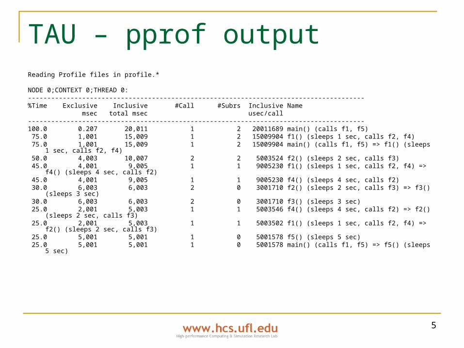
TAU – pprof outputReading Profile files in profile.*

NODE 0;CONTEXT 0;THREAD 0:---------------------------------------------------------------------------------------%Time Exclusive Inclusive #Call #Subrs Inclusive Name msec total msec usec/call---------------------------------------------------------------------------------------100.0 0.207 20,011 1 2 20011689 main() (calls f1, f5) 75.0 1,001 15,009 1 2 15009904 f1() (sleeps 1 sec, calls f2, f4) 75.0 1,001 15,009 1 2 15009904 main() (calls f1, f5) => f1() (sleeps

1 sec, calls f2, f4) 50.0 4,003 10,007 2 2 5003524 f2() (sleeps 2 sec, calls f3) 45.0 4,001 9,005 1 1 9005230 f1() (sleeps 1 sec, calls f2, f4) =>

f4() (sleeps 4 sec, calls f2) 45.0 4,001 9,005 1 1 9005230 f4() (sleeps 4 sec, calls f2) 30.0 6,003 6,003 2 0 3001710 f2() (sleeps 2 sec, calls f3) => f3()

(sleeps 3 sec) 30.0 6,003 6,003 2 0 3001710 f3() (sleeps 3 sec) 25.0 2,001 5,003 1 1 5003546 f4() (sleeps 4 sec, calls f2) => f2()

(sleeps 2 sec, calls f3) 25.0 2,001 5,003 1 1 5003502 f1() (sleeps 1 sec, calls f2, f4) =>

f2() (sleeps 2 sec, calls f3) 25.0 5,001 5,001 1 0 5001578 f5() (sleeps 5 sec) 25.0 5,001 5,001 1 0 5001578 main() (calls f1, f5) => f5() (sleeps

5 sec)

6

TAU – paraprof

7

Paradyn Metrics recorded

Number of CPUs, number of active threads, CPU and inclusive CPU time

Function calls to and by Synchronization (# operations, wait time, inclusive wait time) Overall communication (# messages, bytes sent and received),

collective communication (# messages, bytes sent and received), point-to-point communication (# messages, bytes sent and received)

I/O (# operations, wait time, inclusive wait time, total bytes) All metrics recorded as “time histograms” (fixed-size data

structure) Profiled entities

Functions only (but includes functions linked to in existing libraries)

8

Paradyn Visualizations

Time histograms Tables Barcharts “Terrains” (3-D histograms)

9

Paradyn – time histograms

10

Paradyn – terrain plot (histogram across multiple hosts)

11

Paradyn – table (current metric values)

12

Paradyn – bar chart (current or average metric values)

13

MPE/Jumpshot Metrics collected

MPI message send time, receive time, size, message sender/recipient

User-defined event entry & exit Profiled entities

All MPI functions Functions or regions via manual instrumentation

and custom events Visualization

Jumpshot: timeline view (space-time diagram overlaid on Gantt chart), histogram

14

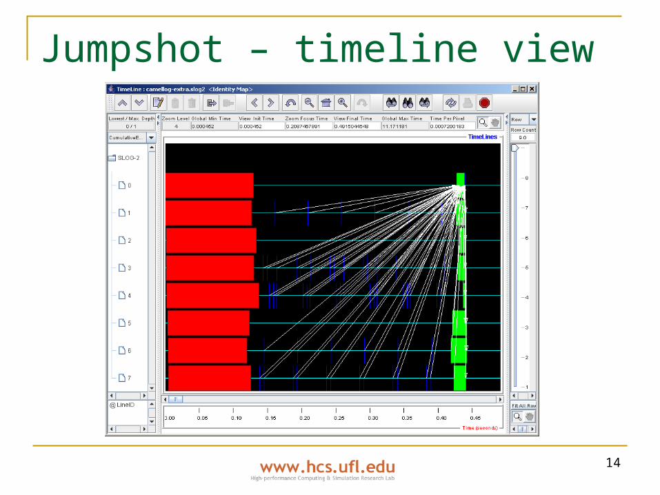
Jumpshot – timeline view

15

Jumpshot – histogram view

16

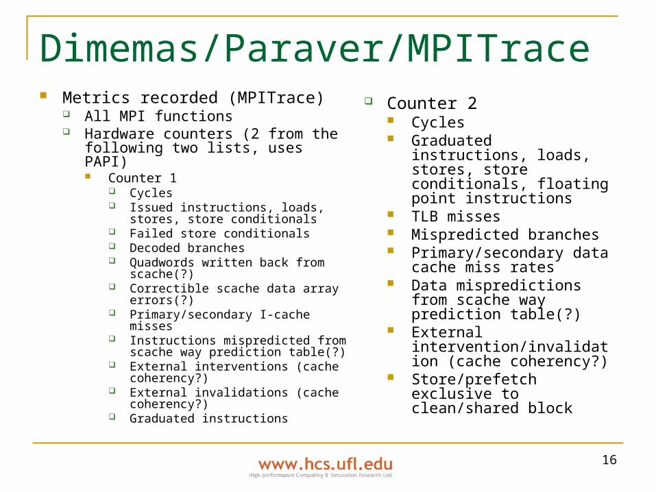
Dimemas/Paraver/MPITrace Metrics recorded (MPITrace)

All MPI functions Hardware counters (2 from the

following two lists, uses PAPI) Counter 1

Cycles Issued instructions, loads, stores,

store conditionals Failed store conditionals Decoded branches Quadwords written back from

scache(?) Correctible scache data array

errors(?) Primary/secondary I-cache misses Instructions mispredicted from

scache way prediction table(?) External interventions (cache

coherency?) External invalidations (cache

coherency?) Graduated instructions

Counter 2 Cycles Graduated instructions,

loads, stores, store conditionals, floating point instructions

TLB misses Mispredicted branches Primary/secondary data

cache miss rates Data mispredictions from

scache way prediction table(?)

External intervention/invalidation (cache coherency?)

Store/prefetch exclusive to clean/shared block

17

Dimemas/Paraver/MPITrace Profiled entities (MPITrace)

All MPI functions (message start time, message end time, message size, message recipient/sender)

User regions/functions via manual instrumentation Visualization

Timeline display (like Jumpshot) Shows Gantt chart and messages Also can overlay hardware counter information

Clicking on timeline brings up a text listing of events near where you clicked

1D/2D analysis modules

18

Paraver – timeline (standard)

19

Paraver – timeline (HW counter)

20

Paraver – text module

21

Paraver – 1D analysis

22

Paraver – 2D analysis

23

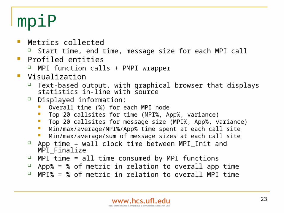
mpiP Metrics collected

Start time, end time, message size for each MPI call Profiled entities

MPI function calls + PMPI wrapper Visualization

Text-based output, with graphical browser that displays statistics in-line with source

Displayed information: Overall time (%) for each MPI node Top 20 callsites for time (MPI%, App%, variance) Top 20 callsites for message size (MPI%, App%, variance) Min/max/average/MPI%/App% time spent at each call site Min/max/average/sum of message sizes at each call site

App time = wall clock time between MPI_Init and MPI_Finalize MPI time = all time consumed by MPI functions App% = % of metric in relation to overall app time MPI% = % of metric in relation to overall MPI time

24

mpiP – graphical view

25

Dynaprof Metrics collected

Wall clock time or PAPI metric for each profiled entity

Collects inclusive, exclusive, and 1-level call tree % information

Profiled entities Functions (dynamic instrumentation)

Visualizations Simple text-based Simple GUI (shows same info as text-based)

26

Dynaprof – output[leko@eta-1 dynaprof]$ wallclockrpt lu-1.wallclock.16143

Exclusive Profile.

Name Percent Total Calls

------------- ------- ----- -------

TOTAL 100 1.436e+11 1

unknown 100 1.436e+11 1

main 3.837e-06 5511 1

Inclusive Profile.

Name Percent Total SubCalls

------------- ------- ----- -------

TOTAL 100 1.436e+11 0

main 100 1.436e+11 5

1-Level Inclusive Call Tree.

Parent/-Child Percent Total Calls

------------- ------- ----- --------

TOTAL 100 1.436e+11 1

main 100 1.436e+11 1

- f_setarg.0 1.414e-05 2.03e+04 1

- f_setsig.1 1.324e-05 1.902e+04 1

- f_init.2 2.569e-05 3.691e+04 1

- atexit.3 7.042e-06 1.012e+04 1

- MAIN__.4 0 0 1

27

KOJAK Metrics collected

MPI: message start time, receive time, size, message sender/recipient

Manual instrumentation: start and stop times 1 PAPI metric / run (only FLOPS and L1 data misses

visualized) Profiled entities

MPI calls (MPI wrapper library) Function calls (automatic instrumentation, only available on

a few platforms) Regions and function calls via manual instrumentation

Visualizations Can export traces to Vampir trace format (see ICT) Shows profile and analyzed data via CUBE (described on

next few slides)

28

CUBE overview: simple description Uses a 3-pane approach to display

information Metric pane Module/calltree pane

Right-clicking brings up source code location

Location pane (system tree) Each item is displayed along with a

color to indicate severity of condition Severity can be expressed 4 ways

Absolute (time) Percentage Relative percentage (changes

module & location pane) Comparative percentage

(differences between executions)

Despite documentation, interface is actually quite intuitive

29

CUBE example: CAMEL

After opening the .cube file (default metric shown = absolute time take in seconds)

30

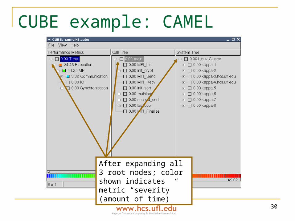
CUBE example: CAMEL

After expanding all 3 root nodes; color shown indicates metric “severity” (amount of time)

31

CUBE example: CAMEL

Selecting “Execution” shows execution time, broken down into part of code & machine

32

CUBE example: CAMEL

Selecting mainloop adjusts system tree to only show time spent in mainloop per each processor

33

CUBE example: CAMEL

Expanded nodes show exclusive metric (only time spent by node)

34

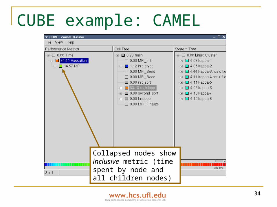
CUBE example: CAMEL

Collapsed nodes show inclusive metric (time spent by node and all children nodes)

35

CUBE example: CAMEL

Metric pane also shows detected bottlenecks; here, shows “Late Sender” in MPI_Recv within main spread across all nodes

36

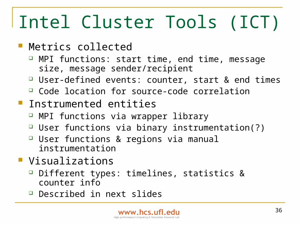
Intel Cluster Tools (ICT) Metrics collected

MPI functions: start time, end time, message size, message sender/recipient

User-defined events: counter, start & end times Code location for source-code correlation

Instrumented entities MPI functions via wrapper library User functions via binary instrumentation(?) User functions & regions via manual instrumentation

Visualizations Different types: timelines, statistics & counter info Described in next slides

37

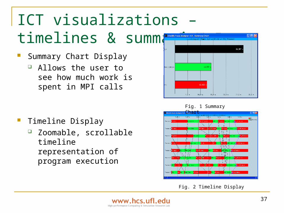
ICT visualizations – timelines & summaries Summary Chart Display

Allows the user to see how much work is spent in MPI calls

Timeline Display Zoomable, scrollable

timeline representation of program execution

Fig. 1 Summary Chart

Fig. 2 Timeline Display

38

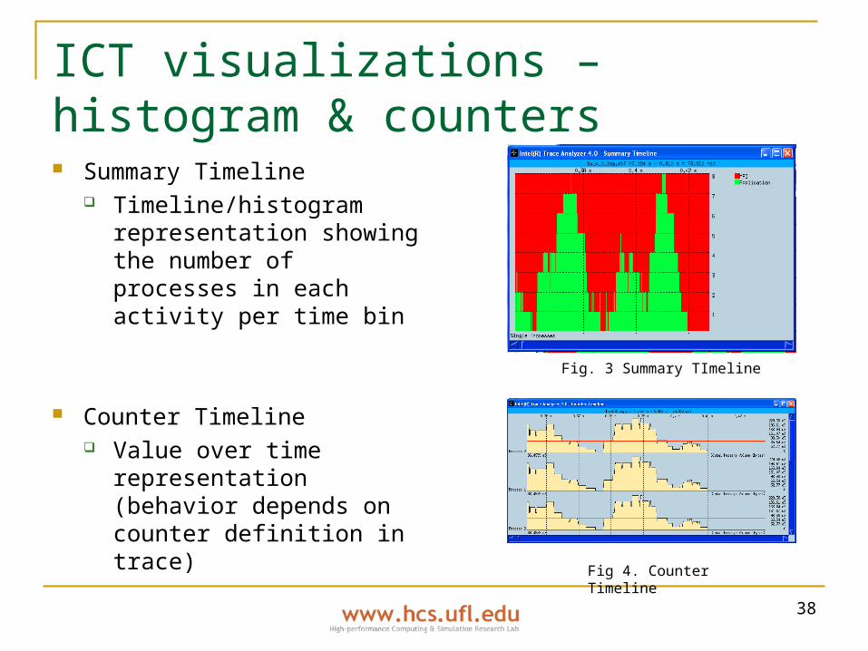
ICT visualizations – histogram & counters Summary Timeline

Timeline/histogram representation showing the number of processes in each activity per time bin

Counter Timeline Value over time

representation (behavior depends on counter definition in trace)

Fig. 3 Summary TImeline

Fig 4. Counter Timeline

39

ICT visualizations – message stats & process profiles Message Statistics Display

Message data to/from each process (count,length, rate, duration)

Process Profile Display Per process data regarding

activities

Fig. 5 Message Statistics

Fig. 6 Process Profile Display

40

ICT visualizations – general stats & call tree Statistics Display

Various statistics regarding activities in histogram, table, or text format

Call Tree Display

Fig. 7 Statistics Display

Fig. 8 Call Tree Display

41

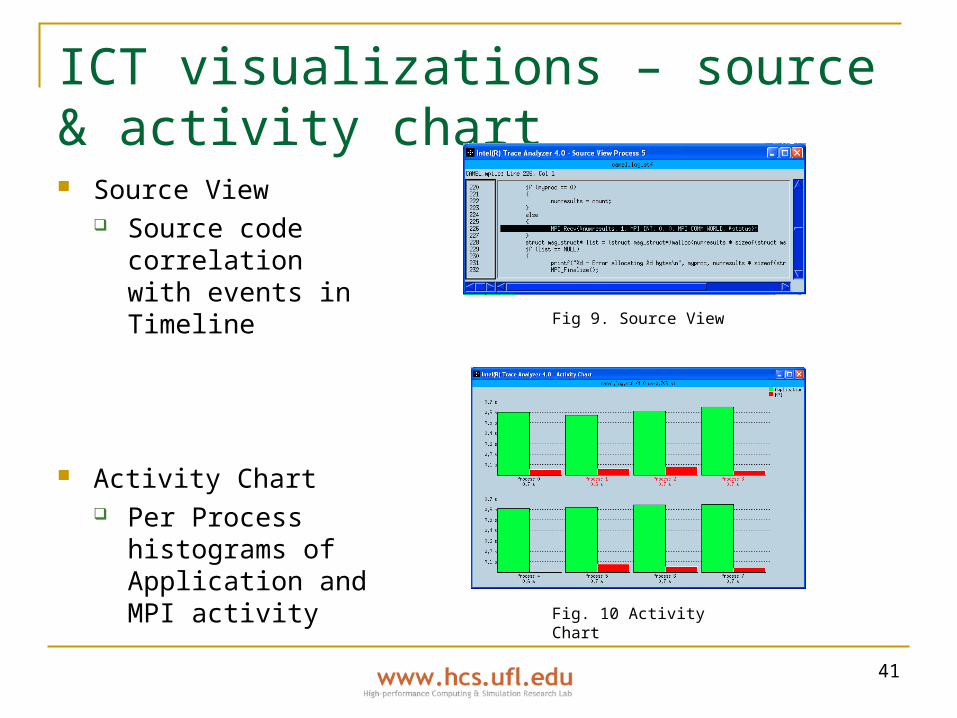
ICT visualizations – source & activity chart Source View

Source code correlation with events in Timeline

Activity Chart Per Process

histograms of Application and MPI activity

Fig 9. Source View

Fig. 10 Activity Chart

42

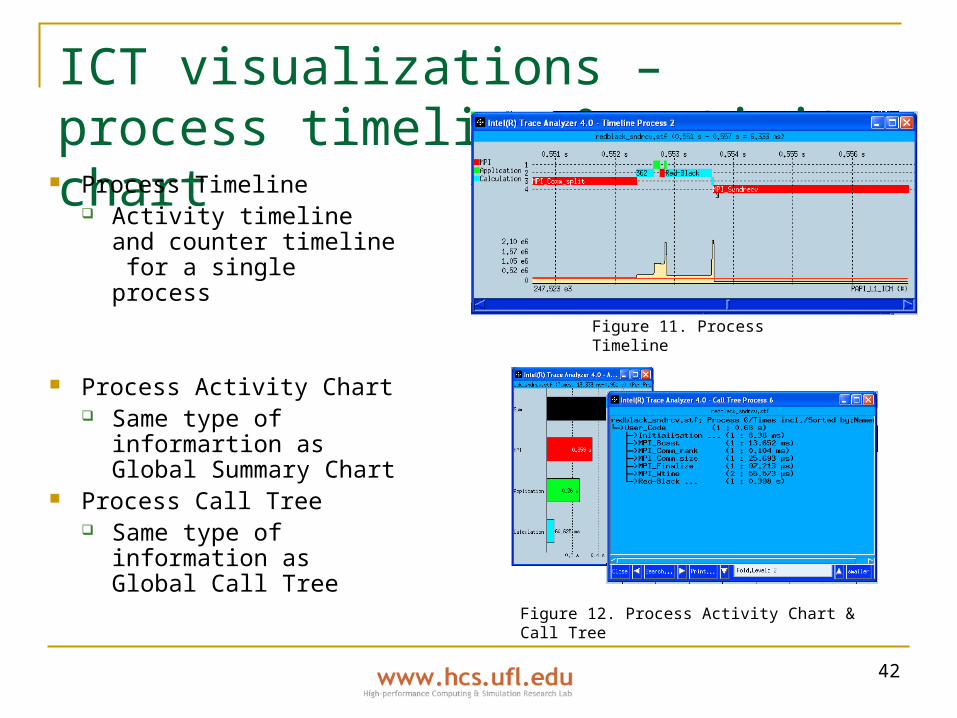
ICT visualizations – process timeline & activity chart

Process Timeline Activity timeline and

counter timeline for a single process

Process Activity Chart Same type of

informartion as Global Summary Chart

Process Call Tree Same type of

information as Global Call Tree

Figure 11. Process Timeline

Figure 12. Process Activity Chart & Call Tree

43

Pablo Metrics collected

Time inclusive/exclusive of a function Hardware counters via PAPI Summary metrics computed from timing info

Min/max/avg/stdev/count

Profiled entities Functions, function calls, and outer loops All selected via GUI

Visualizations Displays derived summary metrics color-coded and inline

with source code Shown on next slide

44

SvPablo

45

MPICL/Paragraph

Metrics collected MPI functions: start time, end time, message size, message

sender/recipient Manual instrumentation: start time, end time, “work” done

(up to user to pass this in) Profiled entities

MPI function calls via PMPI interface User functions/regions via manual instrumentation

Visualizations Many, separated into 4 categories: utilization,

communication, task, “other” Described in following slides

46

ParaGraph visualizations Utilization visualizations

Display rough estimate of processor utilization Utilization broken down into 3 states:

Idle – When program is blocked waiting for a communication operation (or it has stopped execution) Overhead – When a program is performing communication but is not blocked (time spent within MPI library) Busy – if execution part of program other than communication

“Busy” doesn’t necessarily mean useful work is being done since it assumes (not communication) := busy

Communication visualizations Display different aspects of communication Frequency, volume, overall pattern, etc. “Distance” computed by setting topology in options menu

Task visualizations Display information about when processors start & stop tasks Requires manually instrumented code to identify when processors start/stop tasks

Other visualizations Miscellaneous things

47

Utilization visualizations – utilization count

Displays # of processors in each state at a given moment in time

Busy shown on bottom, overhead in middle, idle on top

48

Utilization visualizations – Gantt chart

Displays utilization state of each processor as a function of time

49

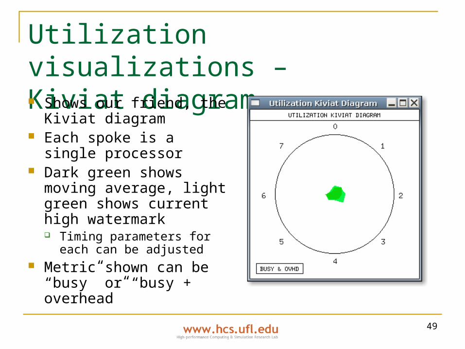
Utilization visualizations – Kiviat diagram Shows our friend, the

Kiviat diagram Each spoke is a single

processor Dark green shows moving

average, light green shows current high watermark Timing parameters for each

can be adjusted Metric shown can be

“busy” or “busy + overhead”

50

Utilization visualizations – streak

Shows “streak” of state Similar to winning/losing

streaks of baseball teams

Win = overhead or busy Loss = idle

Not sure how useful this is

51

Utilization visualizations – utilization summary

Shows percentage of time spent in each utilization state up to current time

52

Utilization visualizations – utilization meter

Shows percentage of processors in each utilization state at current time

53

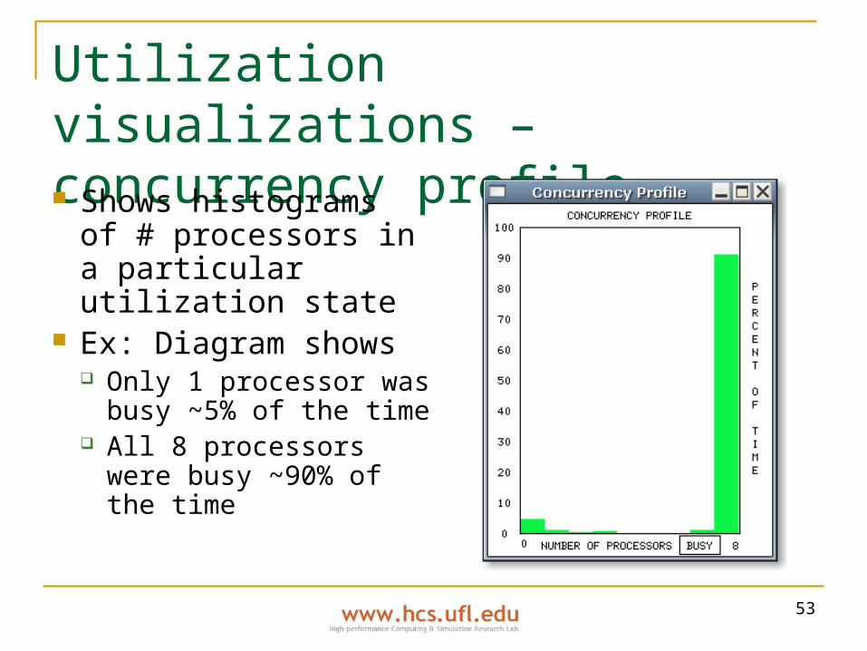
Utilization visualizations – concurrency profile Shows histograms of

# processors in a particular utilization state

Ex: Diagram shows Only 1 processor was

busy ~5% of the time All 8 processors were

busy ~90% of the time

54

Communication visualizations – color code

Color code controls colors used on most communication visualizations

Can have color indicate message sizes, message distance, or message tag Distance computed by topology set in options menu

55

Communication visualizations – communication traffic

Shows overall traffic at a given time Bandwidth used, or Number of messages in flight

Can show single node or aggregate of all nodes

56

Communication visualizations – spacetime diagram

Shows standard space-time diagram for communication Messages sent from node to node at which times

57

Communication visualizations – message queues

Shows data about message queue lengths Incoming/outgoing Number of bytes queued/number of messages queued

Colors mean different things Dark color shows current moving average Light color shows high watermark

58

Communication visualizations – communication matrix Shows which

processors sent data to which other processors

59

Communication visualizations – communication meter Show percentage of

communication used at the current time

Message count or bandwidth 100% = max # of messages /

max bandwidth used by the application at a specific time

60

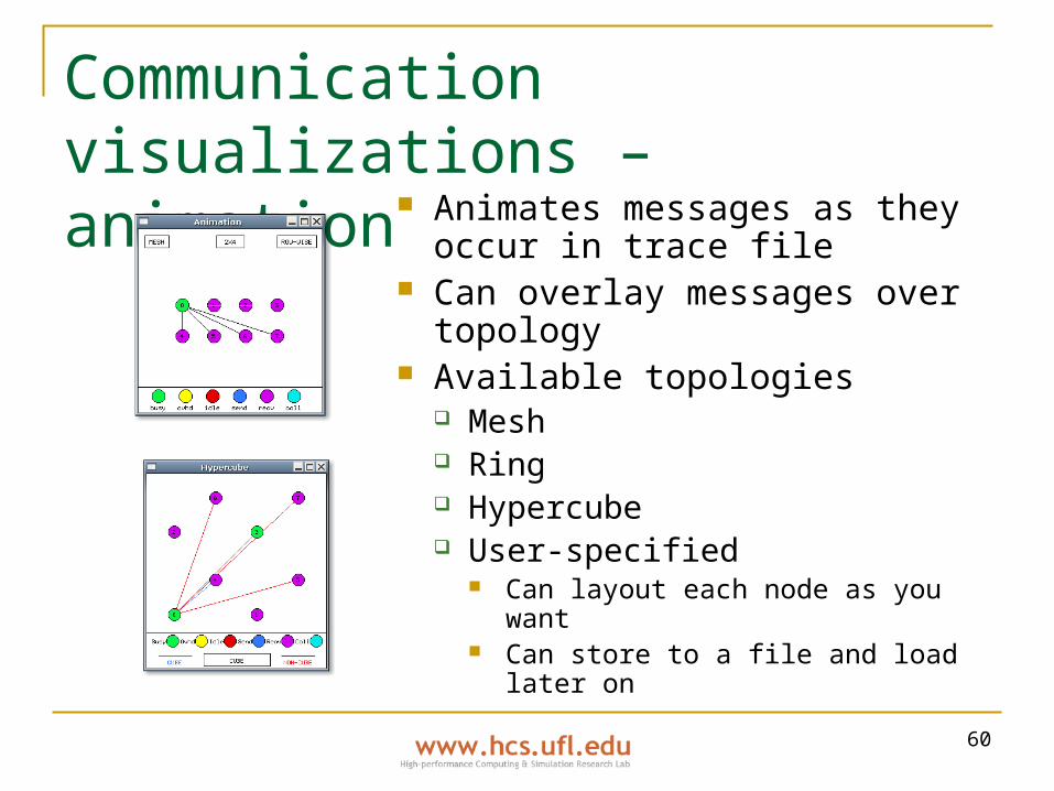
Communication visualizations – animation Animates messages as they

occur in trace file Can overlay messages over

topology Available topologies

Mesh Ring Hypercube User-specified

Can layout each node as you want Can store to a file and load later on

61

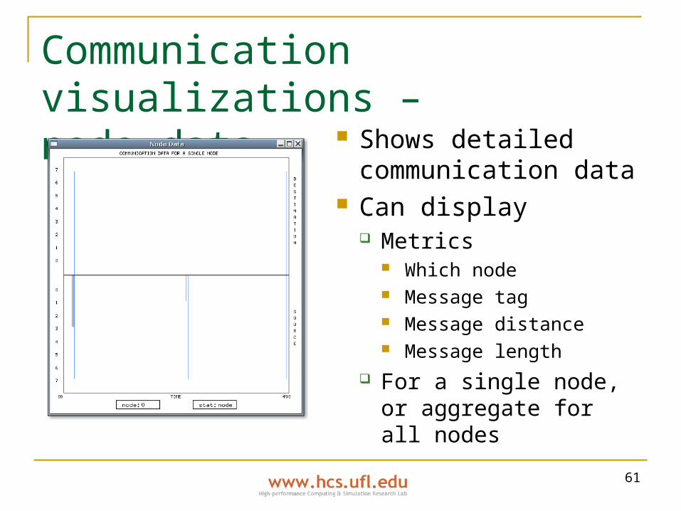
Communication visualizations – node data Shows detailed

communication data Can display

Metrics Which node Message tag Message distance Message length

For a single node, or aggregate for all nodes

62

Task visualizations – task count

Shows number of processors that are executing a task at the current time

At end of run, changes to show summary of all tasks

63

Task visualizations – task Gantt

Shows Gantt chart of which task each processor was working on at a given time

64

Task visualizations – task speed

Similar to Gantt chart, but displays “speed” of each task Must record work done by task in instrumentation call (not

done for example shown above)

65

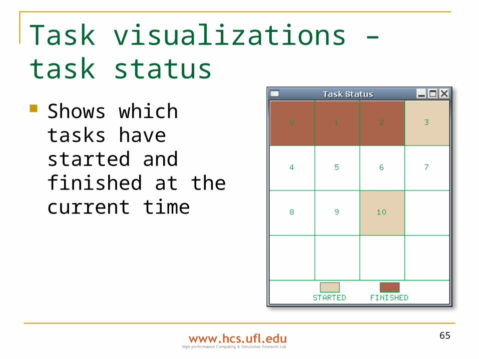
Task visualizations – task status Shows which tasks

have started and finished at the current time

66

Task visualizations – task summary

Shows % time spent on each task Also shows any overlap between tasks

67

Task visualizations – task surface

Shows time spent on each task by each processor

Useful for seeing load imbalance on a task-by-task basis

68

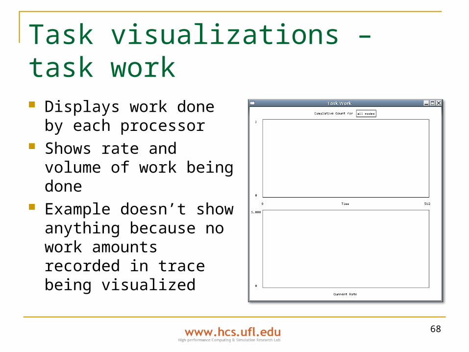
Task visualizations – task work Displays work done by

each processor Shows rate and volume

of work being done Example doesn’t show

anything because no work amounts recorded in trace being visualized

69

Other visualizations – clock, coordinates Clock

Shows current time Coordinate information

Shows coordinates when you click on any visualization

70

Other visualizations – critical path

Highlights critical path in space-time diagram in red Longest serial path shown in red Depends on point-to-point communication (collective can screw it

up)

71

Other visualizations – phase portrait Shows relationship

between processor utilization and communication usage

72

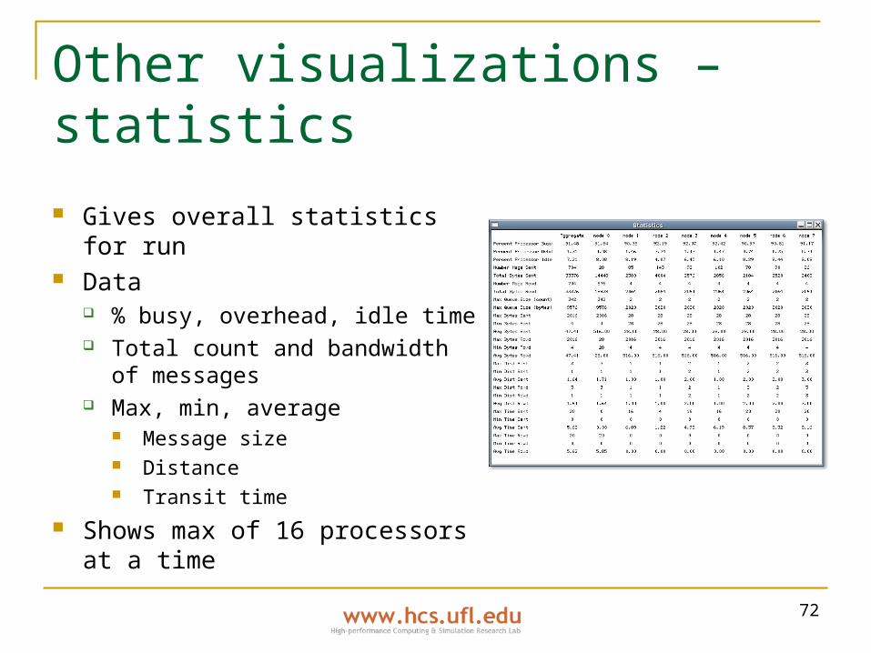
Other visualizations – statistics

Gives overall statistics for run Data

% busy, overhead, idle time Total count and bandwidth of

messages Max, min, average

Message size Distance Transit time

Shows max of 16 processors at a time

73

Other visualizations – processor status Shows

Processor status Which task each

processor is executing Communication (sends

& receives) Each processor is a

square in the grid (8-processor example shown)

74

Other visualizations – trace events

Shows text output of all trace file events