tony prato h.a. cowden professor division of applied social sciences university of missouri...
TRANSCRIPT
Tony PratoTony PratoH.A. Cowden ProfessorH.A. Cowden Professor
Division of Applied Social SciencesDivision of Applied Social SciencesUniversity of MissouriUniversity of Missouri
Evaluating Land Use Change Evaluating Land Use Change for Alternative Futures in for Alternative Futures in
Northwest MontanaNorthwest Montana

Global ChangeGlobal Change
• There are two major components of global change: climate change and land use change.
• Global change reduces biodiversity, modifies hydrological systems, and alters global biogeochemical cycles all of which have significant impacts on human and natural systems.

Extent of Land Use ChangeExtent of Land Use Change
• During the last three centuries, nearly
1.2 million km2 of forest and woodland and
5.6 million km2 of grassland and pasture have been converted to developed land uses on a global basis.
• Between 1982 and 1997, 121,000 km2 of non-federal land in the U.S. were converted to urban uses.

• Through its impacts on the quantity and quality of fish and wildlife habitat, land use change has contributed to the dramatic 1,000-fold increase in species extinction that occurred during the past 400 years.

Research ProjectResearch Project
Assessing Ecological Economic Assessing Ecological Economic Impacts of Landscape Change in Impacts of Landscape Change in
Montana’s Flathead County Montana’s Flathead County

ContributorsContributors• Tony Prato (PI), Kris Dolle, and Yan Barnett, Center
for Applied Research and Environmental Systems, University of Missouri (economics and geography)
• Anthony Clark, Associate Professor of Economics, Lindenwood University, Missouri (economics)
• Ramanathan Sugumaran, Department of Geography, University of Northern Iowa (geography)
• Dan Fagre and Greg Pederson, USGS Northern Rocky Mountain Science Center (ecology)

Objectives of StudyObjectives of Study
• Simulate the economic and land use impacts of alternative economic growth-land use policy futures for Flathead County, Montana.
• Assess the impacts of the simulated future changes in land use on wildlife habitat.
• My presentation will focus on the first objective.

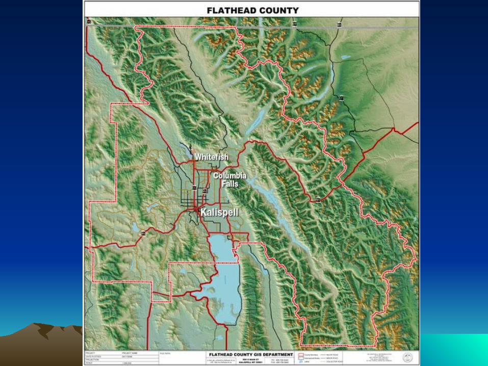
Study AreaFlathead County, Montana


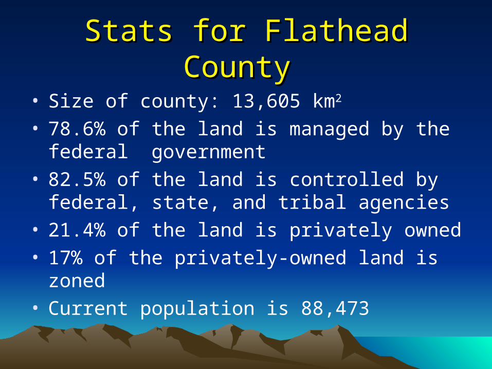
Stats for Flathead County Stats for Flathead County
• Size of county: 13,605 km2
• 78.6% of the land is managed by the federal government
• 82.5% of the land is controlled by federal, state, and tribal agencies
• 21.4% of the land is privately owned • 17% of the privately-owned land is zoned• Current population is 88,473

• 810,000 ha are forested• 405,000 ha are designated
wilderness• Flathead Valley’s elevation is 914
m• The tallest mountain peaks are at
about 3,050 m.

Natural ResourcesNatural ResourcesBob Marshall-Great Bear-Scapegoat Wilderness complex, Flathead National Forest, and the west side of Glacier National Park.
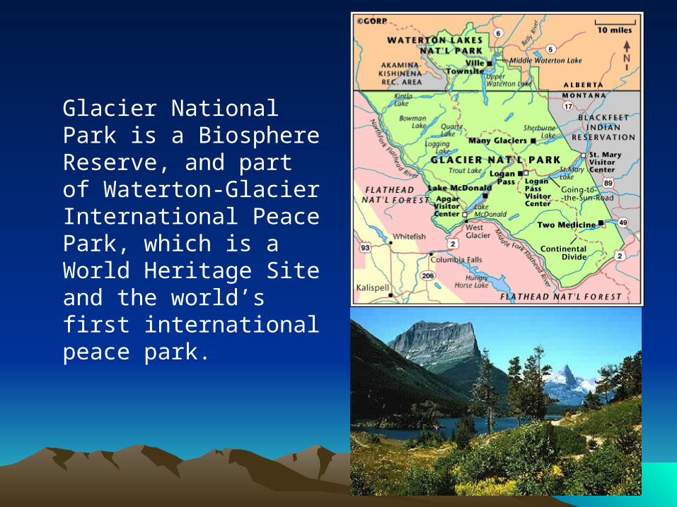
Glacier National Park is a Biosphere Reserve, and part of Waterton-Glacier International Peace Park, which is a World Heritage Site and the world’s first international peace park.

Despite its temperate climate, the county contains a highly diverse flora and fauna with 300 species of aquatic insects, 22 native and introduced species of fish, and nearly all of the large mammals of North America.

Threatened and Threatened and Endangered SpeciesEndangered Species
• Threatened species– grizzly bear– Canada lynx– bull trout– water howellia– spalding catchfly
• Endangered species– whooping crane– gray wolf

Importance of Open SpaceImportance of Open SpaceA 2002 attitudinal survey of Kalispell residents indicated that 42% of the respondents agreed with the statement that there is adequate undeveloped open space in the community; 76% indicated they were concerned about the potential loss of existing open space.
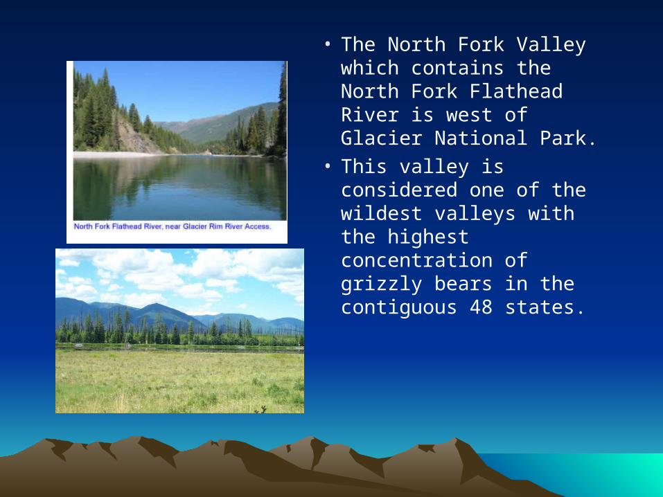
• The North Fork Valley which contains the North Fork Flathead River is west of Glacier National Park.
• This valley is considered one of the wildest valleys with the highest concentration of grizzly bears in the contiguous 48 states.
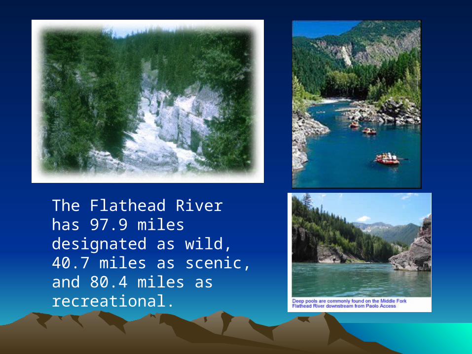
The Flathead River has 97.9 miles designated as wild, 40.7 miles as scenic, and 80.4 miles as recreational.

Flathead Lake is one of the 300 largest lakes in the world and the largest body of freshwater in the western United States.

EconomyEconomy
• Historically, the Flathead economy was highly dependent on extractive resource industries, including lumber and wood products, agriculture, and mining.
• Labor earnings in those industries dropped from a high of $97 million in 1993 to $75 million in 2000.

• Tourism and outdoor recreation are major sources of income and employment in the county.
• 40% of all personal income is the county comes from non-labor sources (i.e., transfer payments from investments, retirement accounts, and social security).
• Overall, the economy has been strong and continues to grow due to a steady wave of new migrants and seasonal residents that are attracted to the area because of its abundant environmental amenities and quality of life.

• Per capita and median incomes have been steadily rising, poverty is falling, and unemployment was at a 30-year low before the current recession.

Flathead Valley

• Flathead Valley and outlying areas are losing open space due to land development.
• Much of the developed land was previously in agricultural uses.
• In the last 30 years, 42,998 ha of farmland in Flathead Valley have been converted to developed uses.

Methods Used in StudyMethods Used in Study• Remote sensing• Land cover classification• Geographic information systems• Land use change analysis• Alternative futures analysis• Economic impact analysis• Surveys

Alternative Futures AnalysisAlternative Futures Analysis
• It is difficult for planners and stakeholders to foresee the potential ecological and economic consequences of their choices, policies, and plans because no one knows for sure what the future will bring.
• Since no single vision of the future is accurate or
superior to others, it is useful to model a set of alternative futures for a region that encompasses a spectrum of possible futures.

• Alternative futures analysis allows a community to assess the possible ecosystem and economic consequences of alternative assumptions about future growth and development.

Other ApplicationsOther Applications• Monroe County, PA• Region of Camp Pendleton, CA• Willamette River Basin, Oregon• Southern Rocky Mountains, AL• Mojave Desert, CA• Northern Highlands Lake District of Wisconsin • Iowa Corn Belt• Upper San Pedro River Basin, AZ and Sonora
(Mexico)• Utah’s Wasatch Front
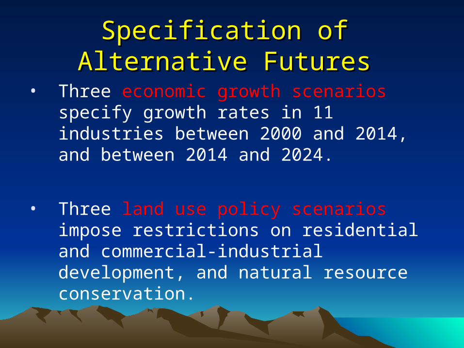
Specification of Alternative FuturesSpecification of Alternative Futures
• Three economic growth scenarios specify growth rates in 11 industries between 2000 and 2014, and between 2014 and 2024.
• Three land use policy scenarios impose restrictions on residential and commercial-industrial development, and natural resource conservation.
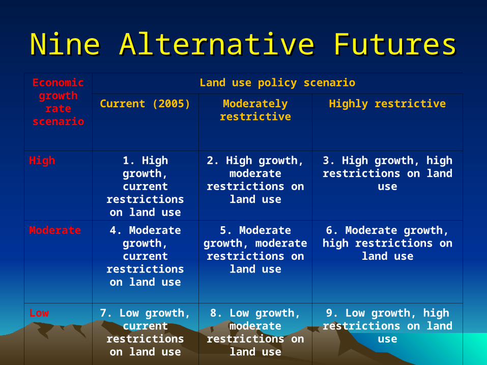
Nine Alternative FuturesNine Alternative FuturesEconomic
growth rate
scenario
Land use policy scenario
Current (2005) Moderately restrictive
Highly restrictive
High 1. High growth, current
restrictions on land use
2. High growth, moderate
restrictions on land use
3. High growth, high restrictions on land use
Moderate 4. Moderate growth, current restrictions on
land use
5. Moderate growth, moderate
restrictions on land use
6. Moderate growth, high restrictions on land use
Low 7. Low growth, current
restrictions on land use
8. Low growth, moderate
restrictions on land use
9. Low growth, high restrictions on land use
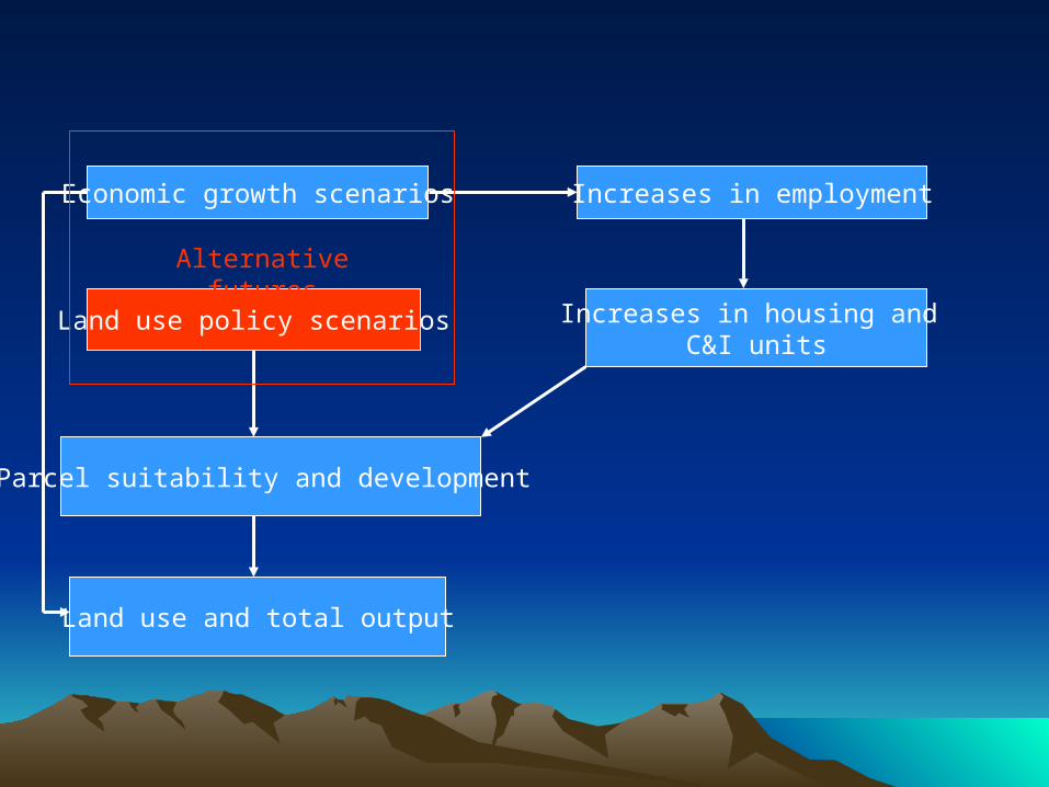
Ecosystem Landscape Ecosystem Landscape Modeling System (ELMS)Modeling System (ELMS)
ELMS simulates the economic and land use impacts of the conversion of land from undeveloped uses to developed uses for the nine alternative futures.

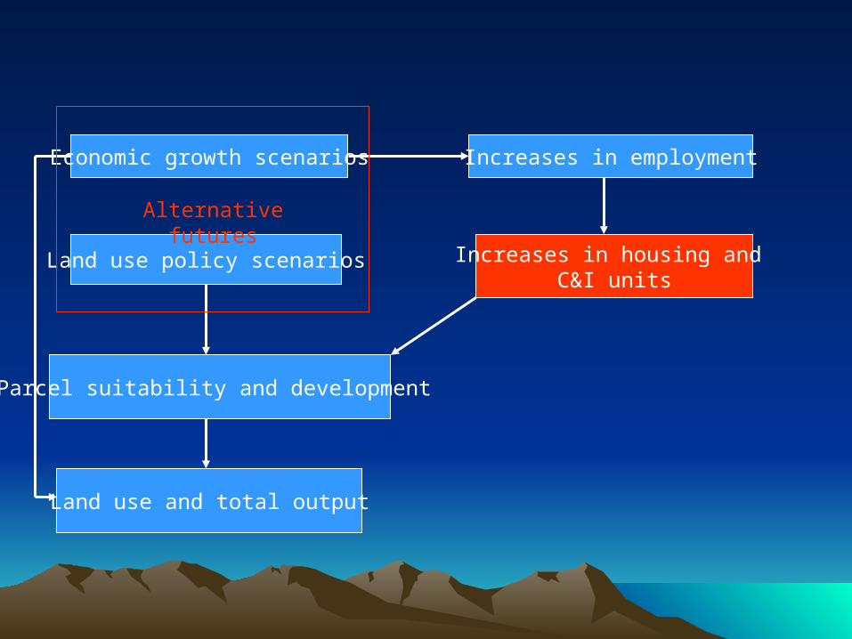
Overview of ELMSOverview of ELMS
Economic growth scenarios Increases in employment
Increases in housing and C&I units
Land use policy scenarios
Parcel suitability and development
Land use and total output
Alternative futures

Economic growth scenarios Increases in employment
Increases in housing and C&I units
Land use policy scenarios
Parcel suitability and development
Land use and total output
Alternative futures

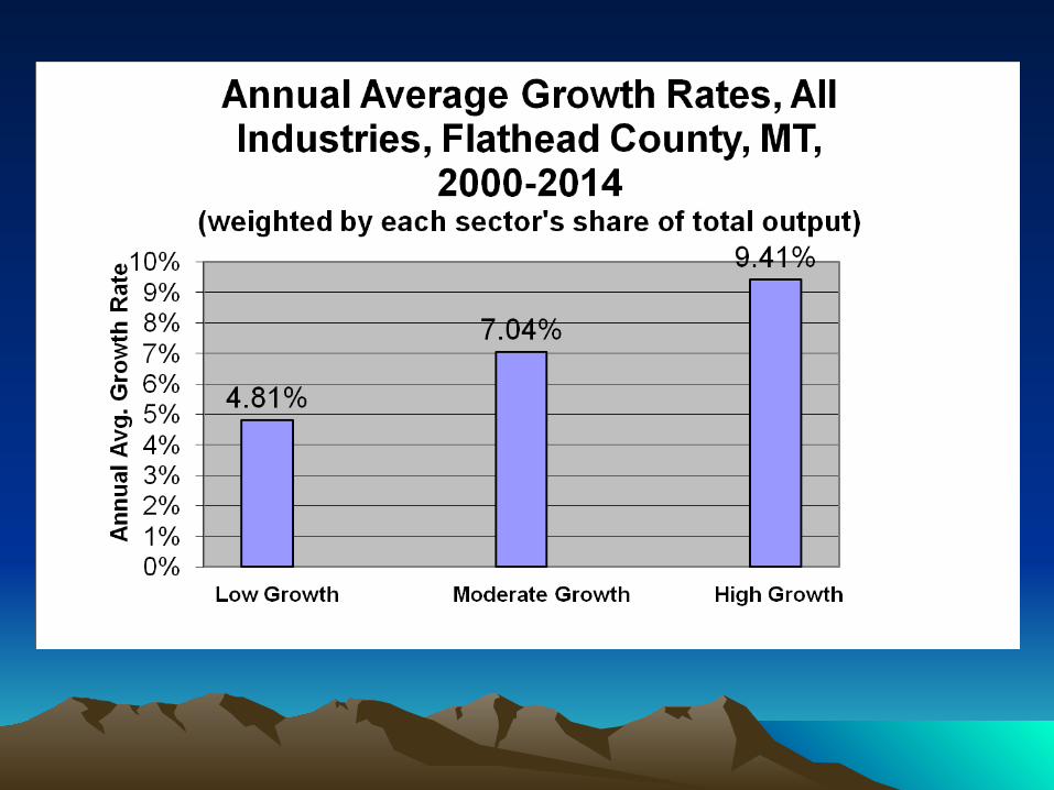
Industry Annual average percentage growth rates
High Moderate Low
Farming and Ranching 0.25 0.22 0.15
Agricultural, Forestry, and Fishery 0.09 -0.14 -0.32
Mining 16 12 8
Construction 11 8 5
Manufacturing (including forest products)
7 5 3
Transportation, Communications and Public Utilities
4 2 0
Finance, Insurance, and Real Estate 10 8 6
Services 11 9 7
Government 10 8 5
Wholesale Trade 9 5 3
Retail Trade 9 5 3
Scenario Growth Rates:Scenario Growth Rates: 2000-20142000-2014

Scenario Growth Rates: 2014-2024Scenario Growth Rates: 2014-2024 Industry Annual average percentage growth rates
High Moderate Low
Farming and Ranching 0.13 0.11 0.08
Agricultural, Forestry, and Fishery
-0.05 -0.07 -0.16
Mining 8 6 4
Construction 5.5 4 2.5
Manufacturing (including forest products)
3.5 2.5 1.5
Transportation, Communications and Public Utilities
2 1 0
Finance, Insurance, and Real Estate (FIRE)
5 4 3
Services 5.5 4.5 3.5
Government 5 4 2.5
Wholesale Trade 4.5 2.5 1.5
Retail Trade 4.5 2.5 1.5


IMPLAN ModelIMPLAN Model
The IMPLAN model was used to estimate increases in total output and employment for each of the 11 industries between 2000 and 2014 and between 2014 to 2024 for the three growth scenarios.

Estimated Increases in Total OutputEstimated Increases in Total Output(millions of 2000 dollars)
2004-2014 2004-2024
Low Mod. High Low Mod. High
4,708 5,114 5,577 7,388 9,892 13,423

Economic growth scenarios Increases in employment
Increases in housing and C&I units
Land use policy scenarios
Parcel suitability and development
Land use and total output
Alternative futures

• Economic growth rates were used in conjunction with IMPLAN multipliers to estimate the increase in employment for each industry and total employment for the three growth scenarios.
• A productivity adjustment was applied to the multipliers to account for improvements in technology that are likely to occur during the two time periods. The adjustment was based on forecasts of productivity increases published by the U.S. Bureau of Labor Statistics.

Simulated Increases in Total Simulated Increases in Total Employment for Growth ScenariosEmployment for Growth Scenarios
0
50,000
100,000
150,000
200,000
2000-2014 2000-2024
Low
Moderate
High
Economic growth scenarios Increases in employment
Increases in housing and C&I units
Land use policy scenarios
Parcel suitability and development
Land use and total output
Alternative futures
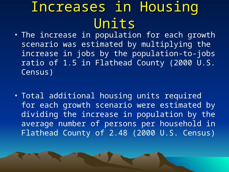
Increases in Housing UnitsIncreases in Housing Units• The increase in population for each growth
scenario was estimated by multiplying the increase in jobs by the population-to-jobs ratio of 1.5 in Flathead County (2000 U.S. Census)
• Total additional housing units required for each growth scenario were estimated by dividing the increase in population by the average number of persons per household in Flathead County of 2.48 (2000 U.S. Census)

Simulated Increases in Total Housing Simulated Increases in Total Housing Units for Growth ScenariosUnits for Growth Scenarios
020,00040,00060,00080,000
100,000120,000140,000
2000-2014 2000-2024
Low
Moderate
High

Increases in C&I AreaIncreases in C&I Area
• The additional area required for new C&I units was estimated by multiplying the increase in total jobs for each growth scenario by the average acreage in C&I land uses per job in Montana of 0.03078 (U.S. Bureau of Economic Analysis, 2000).
Economic growth scenarios Increases in employment
Increases in housing and C&I units
Land use policy scenarios
Parcel suitability and development
Land use and total output
Alternative futures

Land Use Policy ScenariosLand Use Policy Scenarios
• Percent of total housing units in different housing densities
• Area required for each housing density• Setbacks of new houses and C&I units from wetlands
and water bodies• Restrictions on new residential and C&I units in other
environmentally sensitive areas (wetlands, streams, rivers, lakes, ponds, and shallow aquifers)
• Types of development allowed on parcels with and without access to sewers

• Percent of total housing units in each housing density for land use policy scenarios:
Housing Baseline Mod. Restr. Highly Restr. density High 11 17 30 Urban 11 21 28 Suburban 18 21 18 Rural 23 16 9 Exurban 21 13 8 Agricultural 16 12 7
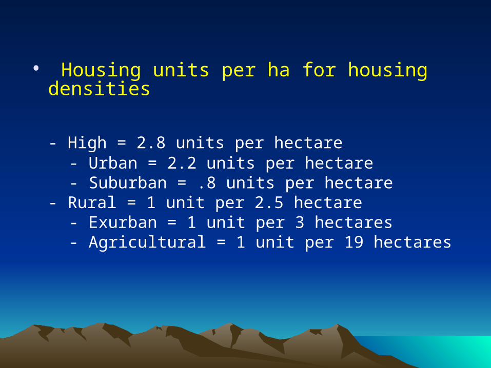
• Housing units per ha for housing densities
- High = 2.8 units per hectare - Urban = 2.2 units per hectare - Suburban = .8 units per hectare
- Rural = 1 unit per 2.5 hectare - Exurban = 1 unit per 3 hectares - Agricultural = 1 unit per 19 hectares

• Setbacks of new housing and C&I units from water bodies for land use policy scenarios:
Policy scenario Setback distance Baseline 6.1 m Moderately restrictive 10.7 m
Highly restrictive 15.2 m

• Treatment of environmentally sensitive areasTreatment of environmentally sensitive areas
The current land use policy scenario imposes no restrictions on the housing densities in environmentally sensitive areas.
The moderately restrictive land use policy scenario allows urban, suburban, rural, exurban, and agricultural densities in a 1.61 km wide buffer area around environmentally sensitive areas.

The highly restrictive land-use policy scenario allows only suburban, rural, exurban, and agricultural densities in a 1.61 km wide buffer area around environmentally sensitive areas.
None of the land use policy scenarios allow the construction of new CI&I units in the buffer areas.

• Development and sewer accessA sewer accessible parcel is located within
the 2003 growth boundaries established for the three incorporated cities (i.e., Columbia Falls, Kalispell, and Whitefish) and the boundaries for the four unincorporated cities (i.e., Bigfork, Evergreen, Hungry Horse, and Lakeside).
Only CI&I, and high, urban, and suburban density housing is allowed on developable, sewer-accessible parcels.

Rural, exurban, and agricultural densities are allowed on any developable parcels.
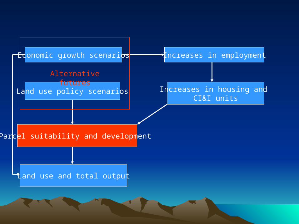
Economic growth scenarios Increases in employment
Increases in housing and CI&I units
Land use policy scenarios
Parcel suitability and development
Land use and total output
Alternative futures

Parcel SuitabilityParcel Suitability
• Suitability of parcels for development was determined based on development attractiveness scores.
• Scores were calculated using a multiple attribute evaluation method that incorporates the attributes of parcels and the weights assigned to those attributes.
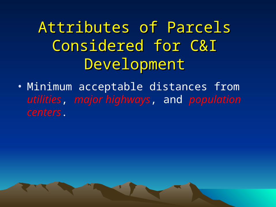
Attributes of Parcels Considered for Attributes of Parcels Considered for C&I DevelopmentC&I Development
• Minimum acceptable distances from utilities, major highways, and population centers.

1. Maximum acceptable distance from utilities
2. Minimum acceptable distance from a major highway
3. Maximum acceptable distance from the edge of town
4. Minimum acceptable distances from eight amenities: mountains, lake, river, preserve, golf course, ski resort, park, and forest
5. The elevation from the valley floor
6. Minimum acceptable distances from seven disamenities: industrial facility or park, mining facility, trailer park, busy highway, commercial center, railroad tracks, and airport
Attributes of Parcels Considered for Residential Development

From the highest to lowest development attractiveness score in the following order of priority:
1. C&I units
2. High density housing units
3. Urban density housing units
4. Suburban density housing units
5. Rural density housing units
6. Exurban density housing units
7. Agricultural density housing units
Order of Parcel DevelopmentOrder of Parcel Development

Economic growth scenarios Increases in employment
Increases in housing and CI&I units
Land use policy scenarios
Parcel suitability and development
Land use and total output
Alternative futures

Land Shortages and SurplusesLand Shortages and Surpluses
• A land shortage occurs when the area available for development is less than the area required for development.
• A land surplus occurs when the area available for development is greater than the area required for development.
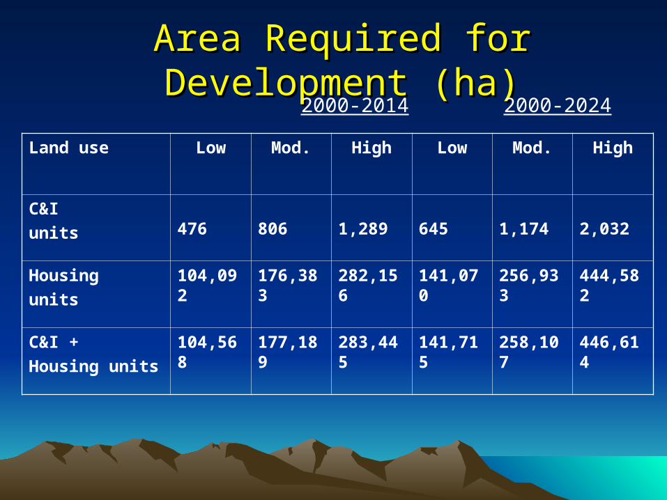
Area Required for Development (ha)Area Required for Development (ha) 2000-2014 2000-2024
Land use Low Mod. High Low Mod. High
C&I
units
476 806 1,289 645 1,174 2,032
Housing
units
104,092 176,383 282,156 141,070 256,933 444,582
C&I +
Housing units
104,568 177,189 283,445 141,715 258,107 446,614

Area DevelopedArea DevelopedCurrent Land Use Policy (ha)Current Land Use Policy (ha) 2000-2014 2000-2024
Land use Low Mod. High Low Mod. High
C&I
units
476 806 1,289 645 1,174 2,032
Housing
units
104,092 176,383 215,641 141,070 215,756 214,898
C&I +
Housing units
104,568 177,189 216,930 141,715 216,930 216,930
Surplus or
Shortage
112,363 39,741 -66,515 75,215 -41,177 -229,683

Area Developed Area Developed Mod. Restrictive Land Use Policy (ha)Mod. Restrictive Land Use Policy (ha)
2000-2014 2000-2024
Land use Low Mod. High Low Mod. High
C&I
units
463 785 1,264 627 1,198 2,036
Housing
units
63,961 108,398 173,600 86,697 157,792 164,309
C&I +
Housing units
64,424 109,182 174,864 87,324 158,989 166,345
Surplus 154,277 109,519 43,837 131,378 59,712 52,357

Area Developed Area Developed Highly Restrictive Land Use Policy (ha) Highly Restrictive Land Use Policy (ha)
2000-2014 2000-2024
Land use Low Mod. High Low Mod. High
C&I
units
464 784 1,257 627 1,155 1,991
Housing
units
32,281 64,893 103,526 51,832 94,365 163,077
C&I +
Housing units
38,745 65,676 104,783 52,460 95,519 165,068
Surplus 172,035 145,103 105,996 158,320 115,260 45,711

2000-2014 2000-2024
Land use Low Mod. High Low Mod. High
C&I
units
112,363 39,741 -66,515 75,215 -41,177 -229,683
Housing
units 154,277 109,519 43,837 131,378 59,712 52,357
C&I +
Housing units 172,035 145,103 105,996 158,320 115,260 45,711
Surplus or
Shortage
112,363 39,741 -66,515 75,215 -41,177 -229,683
Summary of Land Surpluses and Summary of Land Surpluses and Shortages (ha)Shortages (ha)

Interpretation of ResultsInterpretation of Results
• Whether land surpluses or land shortages occur depends on the alternative future.
• Although land shortages decrease as economic growth decreases, it is not politically feasible to control growth in Flathead County.
• Continuation of current (2005) land-use policy can lead to land shortages in the period 2000-2014 with the high growth scenario, and in the period 2014-2024 with the moderate and high growth scenarios.
• It appears that potential land shortages can be alleviated by implementing a more restrictive land use policy.
CaveatsCaveats• As land requirements for new housing and C&I
units approach the remaining amount of developable land, land prices would increase.
• Higher land prices would alleviate land shortages.
• Higher land prices would drive up housing costs, decrease housing affordability, and adversely impact limited-income families.

PublicationsPublications
Prato, T., A.S. Clark, K. Dolle, and Y. Barnett. 2007. Evaluating alternative economic growth rates and land use policies for Flathead County, Montana. Landscape and Urban Planning 83:327–339.
Prato, T., A. Clark, and Y. Barnett. 2008. Evaluating potential wildlife impacts of future land development adjacent to protected areas. George Wright Forum 25:70-88.
Prato, T. In press. Evaluating tradeoffs between economic and wildlife values associated with future economic growth and development in the Northern Rocky Mountains. Mountain Research and Development.

Spatial Decision Support ToolSpatial Decision Support Toolhttp://projects.cares.missouri.edu/montana/

Questions and Comments
Questions and Comments