WPS6062

POLICY RESEARCH WORKING PAPER 6062

Together We Stand?

Agglomeration in Indian Manufacturing

Ana M. Fernandes

Gunjan Sharma

The World BankDevelopment Research GroupTrade and Integration Team

May 2012

Pub

lic D

iscl

osur

e A

utho

rized

Pub

lic D

iscl

osur

e A

utho

rized

Pub

lic D

iscl

osur

e A

utho

rized

Pub

lic D

iscl

osur

e A

utho

rized

Pub

lic D

iscl

osur

e A

utho

rized

Pub

lic D

iscl

osur

e A

utho

rized

Pub

lic D

iscl

osur

e A

utho

rized

Pub

lic D

iscl

osur

e A

utho

rized

POLICY RESEARCH WORKING PAPER 6062

Abstract

This paper uses plant-level data to examine the impact Second, plants respond differently to policy reformsof industrial and trade policy reforms on the geographic based on their size. Liberalization in foreign directconcentration of manufacturing industries in India investment and de-licensing caused small plants tofrom 1980 to 1999. First, the research shows that de- disperse, while trade liberalization had the opposite effect.licensing and liberalization in foreign direct investment However, for large plants trade liberalization led to lowersignificantly reduced spatial concentration, but trade spatial concentration.reforms had no significant effect on spatial concentration.

Tbis paper is a product of the Trade and Integration Team, Development Research Group. It is part of a larger effort bythe World Bank to provide open access to its research and make a contribution to development policy discussions aroundthe world. Policy Research Working Papers are also posted on the Web at http://econ.worldbank.org. The authors may becontacted at afernandes@worldbank.org and sharmag@missouri.edu.

r he Policy Research Working Paper Series disseminates thefindings ofwork inprogress to encourage the exchange ofideas about development

issues. An objective ofthe series is to get the findings out quickly, even ifthe presentations are less than fully polished. The papers carry the

names ofthe authors and should be cited accordingly. The findings, interpretations, and conclusions expressed in this paper are entirely those

ofthe authors. They do not necessarily represent the views ofthe International Bank for Reconstruction and Development/World Bank and

its affiliated organizations, or those ofthe Executive Directors ofthe World Bank or the governments they represent.

Produced by the Research Support Team

Together We Stand? Agglomeration in Indian

Manufacturing

Ana M. Fernandes*and Gunjan Sharnat

JEL classification:F10, F15, 02, R12. Keywords: Trade, Foreign direct investment, de-

licensing, a , i:i, spatial distribution, India

*World Bank Development Research Group, af ernandes(Dworldbank. orgtUniversity of Missouri, sharmagOmissouri. edu

ýSupport froin the governnents of Norway, Sweden and the United Kingdon through the Multi-DonorTrust Fnd for Trade and Development is - 1 0F,fill·. acknowledged. We would like to thank Devashish Mitraand Hiau Looi Kee as well as seninar participants at Uni-, i-i -. of Missouri, the Midwest Trade Meetings, theIGC Urbanization Conference, the North Anerican Summer Meeting of the Econometrics q.. i, I -., and theWorld Bank. The findings expressed in this paper are those of the authors and do not i., - -- I; representthe views of the World Bank.

1 Introduction

Recent literature has shown that 1I.- tiis and economic density are important drivers

of productivity and economic growth (e.g., Ciccone and Hall (1996), Cingano and Schivardi

(2004), Lall et al. (2004), Brulhart and Sbergami (2009)). However, the clustering of pro-

duction may lead to increased regional concentration of income if labor is imperfectly mobile

(Hanson and Harrison (1999), Topalova (2004)). This in turn may lead to a regional concen-

tration of poverty and increasing inter-regional disparities, particularly when labor mobility

across regions is limited. Both these factors are extremely relevant for India where the spatial

distribution of manufacturing has several interesting and peculiar features.'

Firstly, the distribution of industries across Indian states is highly skewed. In 1985, the

locational gini coefficient for Indian manufacturing was 0.7 as compared to 0.25 for (Ili1. %.

manufacturing. 2 Secondly, the spatial distribution of manufacturing industries in India ex-

perienced significant changes in the 1980s and 1990s. The growth rate of the various states'

share of manufacturing employment exhibits differing trends not only across the two decades

but also across smaller sub-periods. Thirdly, there is significant heterogeneity in - 1-

ation patterns across Indian industries.' Fourth, from 1950 to 1990 industrial policy - in

particular, licensing - was explicitly used by the government to make the spatial distribution

of industry "less unequal". These features gain even more significance in face of the major

'Regional trends in in, 1 dif-. in India have been a cause of concern, particularly in view of the massiveeconomic changes the country experienced since the mid-1980s. Deaton and Dreze (2002) show evidence ofdivergence in per capita consumption across states and of growing urban-rural inequalities, both within andacross states. See Pal and Ghosh (2007) for a detailed review of evidence of increasing regional disparities inIndia.

2For each country, the locational gini coefficient measures the in, I.11 i -. in a measure of regional special-

ization of industry j and its formula is given by qj _ Ginij(rj,) where rj, ,L with Lj, beingz1 L3 ~ in

employment of industry j in geographic area s and L, being total manufacturing employment in geographicarea s, s = 1, ..M. The coefficient for China is taken from Ge (2009) while that for India is the average acrossthe Gini coefficients for 2-digit industries calculated by the authors.

'Unreported figures (available from the authors) show that for example employment shares in the wool,silk and man-made fiber industry (NIC 24) grew at fairly similar rates across Indian states between 1980 and1990 providing no evidence of increasing agglomeration. However from 1990 to 1999, most states experiencednegative growth rates while a handful experienced extremely high positive growth rates of employment shareof this industry. Thus the industry agglomerated from 1990 to 1999. On the other hand, it is difficult tosay whether employment in the chemical and chemical products industry (NIC 30) became relatively moreagglomerated during the 1990s compared to the 1980s. What happened was a change in the i.1], if-. of thestates with high growth rates of employment share of this industry from 1980s to the 1990s.

2

industrial and trade policy reforms and the general shift towards market-oriented economic

policies that occurred in the 1980s and 1990s in India. Theory does not offer clear-cut pre-

dictions regarding the effect of industrial de-licensing, trade liberalization, and foreign direct

investment reforms on spatial concentration of manufacturing industries, and hence the need

for empirical analysis.

In this paper we ask the following questions. What are the determinants of the high level

of spatial concentration in Indian manufacturing? How much of the changes in the spatial

distribution of Indian manufacturing industries can be attributed to policy reforms, after

conditioning on the traditional determinants on 1 1 - endowments, Mlarshallian-

type linkages and knowledge spillovers? Does the spatial distribution of manufacturing plants

of different sizes differ in response to policy changes? To answer these questions, we focus on

indices of geographic concentration of manufacturing industries in India constructed following

Ellison and Glaeser (1997) - henceforth EG indices - based on plant-level data from the Annual

Survey of Industries (ASI) for the period 1980-99.

Our results show that industrial de-licensing has a significant negative impact on geo-

graphic concentration levels (a one standard deviation increase in the proportion of output

de-licensed leads to a 9.; V decline in the EG index) and the same is true for foreign direct

investment (FDI) liberalization (with a one standard deviation increase in the proportion

of industry output open to FDI reducing the average EG index by 10. ). However, our

estimates also show that trade policy has no effect on the spatial concentration of Indian

manufacturing. Further we find that there is significant size-based variation in the response

of concentration to the policy as well as the traditional determinants of :w1iii i:f1ij. De-

licensing and FDI liberalization cause small plants to disperse. Trade policy has no effect on

the concentration of medium-size plants but a one standard deviation decline in the effective

rate of protection leads to a decline in the EG index of large plants and a 2.1 " increase

in the EG index of small plants. Our results are robust to heteroskedasticity-correcting

FGLS techniques and controls for persistence in the h111 i..ij process as well as to a

wide variety of fixed effects and specification tests.

A large literature provides evidence of a significant positive effect of :' economies

on firm-level as well as iiregate-level productivity. Thus, our finding that policy reforms

3

in India raised geographic dispersion would imply that there were productivity losses (or at

the very least, lower productivity gains as a result of the reforms) in Indian manufacturing.

This implication of our results could be one explanation for the finding that only a quarter

of the Indian growth miracle can be attributed to the policy reforms shown by Bollard et al.

(2010). That is, the tendency of Indian manufacturing to disperse after trade and industrial

policy reforms reduced its ability to take advantage of 1.I.-rti:f1i economies, and hence

reduced regate productivity growth.

Our study's contribution to the literature is three-fold. First, our index of :1I.-rti:fvij -

the EG index - provides a detailed picture of spatial concentration at a micro level. Since it is

computed at a relatively disaggregated 3-digit level of industries across Indian states it avoids

problems associated with plants changing product mix (and hence, changing their industrial

classification which would occur if we considered 4-digit industries), and problems associated

with very small geographic units. 4 Second, our study is one of the first that explicitly

controls for and measures the impact of three different policies - industrial de-licensing,

trade reforms, FDI liberalization - in addition to controlling for public sector presence in

Indian manufacturing. Third, unlike other studies which focus on cross-sections or very

short panels, our data spans a 19 year period for approximately 170 industries. Hence, our

measures of industrial and trade policy as well as the proxies for the traditional determinants

of concentration cover a long and interesting time span. They allow us to present a complex

and nuanced picture of the forces that affect spatial concentration. Moreover, the use of

a long panel of industries allows us to control for industry and time fixed effects in our

specifications. Also we are able to lag explanatory variables to account for the slow moving

nature of the determinants of 1.I.-r i..ij. We account for serial correlation by estimating

clustered standard errors. Lastly, to the best of our knowledge our study is the first to

consider EG indices of - h 1 1 .tii for different plant size categories.

The paper is organized as follows. In Section 2 we discuss the measurement of :- i-

eration and the evidence on the traditional determinants of :-1iii i..i. In Section 3

we discuss the policy determinants of :w1iim .ti - de-licensing, trade reforms, and FDI

4 According to Mayer and Mayer (2004) the use of very small geographic units "can lead to an underesti-mation of agglomeration levels since it :, i It-1. separates clusters that sprawl across the border betweenunits".

4

liberalization. In Section 4 we describe and summarize our data. Section 5 presents the es-

timation strategy while Section 6 discusses the results. Section 7 discusses the results using

plant-size-based measures of : h1 .i:'fji. Section 8 presents the results from alternate

specifications. Section 9 concludes.

2 Agglomeration: Measurement and Traditional Deter-

minants

2.1 Measurement of Agglomeration

Several indices can be used to measure the geographic concentration of an industry within

a country: e.g., locational Gini coefficients, Hoover indices and Theil indices. Suppose that

s5j is the share of geographic area s, s = 1, ..M, in industry j's total employment in the

country that is, sj = . Further, x, is the share of geographic area s in total manufac-

turing employment in the country, that is, x, = L. The first measure we consider is a raw

geographic concentration index for each industry j in a given time period which is given by

Gj = EM (sj, - x,) 2 . The index measures the degree to which the geographic pattern of

employment in the industry departs from the geographic pattern of manufacturing employ-

ment in the country as a whole. The index takes a value of zero if industry employment

is uniformly spread across geographic areas. Greater values of the index indicate relatively

stronger geographic w 1 i of the industry. A potential problem with this raw geo-

graphic concentration index is that even if plant location was chosen completely at random it

would by definition be larger in industries including only a small number of very large plants.

Thus Gj could be large solely due to industrial structure.

Hence, the second and main measure we consider is the EG index proposed by Ellison

and Glaeser (1997) which controls for the number and size distribution of plants, i.e., the

impact of the industrial structure. The EG index is the most commonly used index in the

1.-issi i: literature. Ellison and Glaeser (1997) develop a plant location choice model

to analyze geographic concentration at the industry-level that captures both the random

~i1i :1tij- that would be generated if plants chose their location by throwing darts on

5

a board as well as additional i l.in-:itiij caused by localized industry-specific spillovers

and natural advantages. Drawing upon their model they propose an index of geographic

concentration of employment in an industry that controls for industry characteristics, namely

for the size distribution of plants in the industry.' Indeed, one of the key advantages of the

EG index is that it allows for cross-industry comparisons.

Considering the aforementioned raw geographic concentration index Gj for industry jand its plant size distribution as measured by the Herfindahl index, Hj = I 1 z , where zij

is plant i's share in employment of industry j, the EG index for industry j in a given time

period is defined by Equation 1:6

(, - x()2)5(1- _ _1 1. -2 _EN G-2 (1 _ EMX2)Hj( 1- E ZX2) - (1 J - Hj) (1)

The subtraction of the term (1 - EMIx2)Hj in Equation 1 accounts for the aforementioned

problem that Gj would be larger in industries with just a few large plants even if plants

chose their locations randomly. That term corresponds to the level of concentration that

would be expected (in the model of Ellison and Glaeser (1997)) if plants in the industry

chose their locations independently and randomly and both industry-specific spillovers and

natural advantages played no role. Therefore, the EG index measures the concentration

of employment in an industry over and above the level of concentration that would have

prevailed if plants were distributed completely at random. Greater values of the EG index

are associated with greater geographic concentration of the industry.7 Dumais et al. (2002)

show that the index can be generalized to a dynamic setting. Note that we compute the

Herfindahl index Hj based on our plant level data for Indian industries, rather than take

it from external sources as in other studies. This is a particularly important advantage of

5The main prediction of the model is that the relationship between average levels of concentration andindustry characteristics is the same whether concentration is caused by from spillovers, from natural advan-tage, or from a combination of both. This prediction implies that one can construct an index that controlsfor industry differences, regardless of the cause of concentration.

'The Herfindahl index is defined as usual covering all plants in the industry without a geographic dimen-S10n.

'A value of zero for the EG index indicates that industry employment is as concentrated as would beexpected from a random location process. Ellison and I ( - i (1997) suggest that industries with EG indexvalues higher than 0.05 are highly concentrated while those with EG index values below 0.02 are not veryconcentrated.

6

our index since it allows us to compute the Herfindal index at the same level of industrial

disaggregation as the raw geographic concentration index Gj.

2.2 Traditional Determinants of Agglomeration

Mayer and Mayer (2004) and Combes and Overman (2004) review in detail a large number

of studies that analyze the determinants of :-se1 ii ii measured by the rate of growth

of employment of an industry in a particular location or by some ;-1-- 1 ij index for

an industry. These studies focus on knowledge externalities (Glaeser et al. (1992)), labor

pooling (Overman and Puga (2009), Amiti and Cameron (2007)), input networks (Holmes

(1999), Rosenthal and Strange (2001)), demand networks (Hanson (1996), Hanson (1997)),

natural advantage, and increasing returns to scale (Kim (1995), Amiti (1999), Haaland et al.

(1999)) as factors that affect plant location. The intuition behind these various mechanisms

for 1ii is the following.

First, plants will tend to locate in areas that provide localization economies (for example,

areas near raw material suppliers, areas with existing input networks, areas where the supply

of the types of workers that the plant needs is plentiful, areas with good infrastructure) and

urbanization economies (for example, areas where sectors and plants that are a source of

demand for the plant's product are located). This means that an industry which is more

reliant on, say, domestically purchased inputs, or on transportation will tend to locate in areas

that have existing input networks. Thus such industry will tend to be more -1.n.t-

than an industry that is less dependent on inputs and roads.

Second, industries with increasing returns to scale can lower their costs of production

and raise productivity if they locate production in a few locations only. Hence, industries

characterized by increasing returns to scale will tend to be more geographically concentrated

than other industries. However Haaland et al. (1999) argue that while theory provides an

unambiguous prediction that industries characterized by a higher degree of returns to scale

will tend have higher levels of absolute concentration (i.e., when an industry is unequally

distributed across geographic units), no such prediction holds for the case of relative con-

centration. That is, a higher degree of returns to scale may not affect how different the

geographic spread of an industry is relative to the average spread of industries between geo-

7

graphic units. As Mayer and Mayer (2004) report, there is little evidence that the degree of

returns to scale affects -p1ii .irii. In fact, Haaland et al. (1999) find that higher degrees

of economies of scale are associated with lower relative and absolute concentration levels.

Third, plants will also choose location based on dynamic externalities - the Marshall

(1890), Arrow (1962), Romer (1984) or MAR externalities. As plants tend to locate near

one another, the extent of knowledge spillovers increases, leading to greater productivity of

the industry. This results in a higher rate of growth of employment of that industry and

that location. Other dynamic externalities include those modeled by Porter (1991), that

relate the degree of competition in a location to higher innovation and hence to greater

knowledge spillovers and greater concentration, as well as others modeled by Jacobs (1969)

which relate variety and diversity in a location to greater knowledge spillovers, and hence to

greater concentration in that location. Our specification will include controls for all these

traditional determinants of :w1 i.ificpi. as described in Section 5.

3 Policy Determinants of Agglomeration

Before describing in detail the policy reforms in India, we discuss existing evidence regarding

the explicit role of government policy for the geographic concentration of manufacturing.

Lall and Chakravorty (2005, 2007) study the determinants of the location of new private

and public sector industrial investments in India as structural reforms proceeded between

1992 and 1998. Their results show that new private sector industrial investments were biased

towards existing industrial clusters and coastal districts and depended on the size of the

investments in the same location prior to the reforms and on the size of the investments

in neighboring locations as reform proceeded. The authors infer that structural reform led

to increased spatial inequality in terms of industrialization. These studies provide some

interesting and important stylized facts about the location of manufacturing industry in India.

However, due to the nature of the data used they are unable to analyze long-term patterns

and determinants of '-g1iii n.-1i as we do in this paper. Bai et al. (2004) investigate

the evolution of the Hoover index of :- :1 i constructed using Cliij. industry-

level data from 1985 to 1997. They estimate the impact of local protectionism (i.e., the

8

fact that local governments shelter certain industries in the region from competition) on

1.i.t i.. Their results show that industries with high past profit margins and high

shares of state ownership are less geographically concentrated.' Lu and Tao (2009) address

that same question using(Iiii. %.. industry-level data from 1998 to 2005 and show that there is

less geographic concentration in industries with higher shares of employment in state-owned

enterprises. Fujita and Hu (2001) show an increasing income disparity between China's

coastal and interior regions and attribute it to the clustering of manufacturing and the self-

selection of FDI into coastal Special Economic Zones. Ge (2009) demonstrates that access

to foreign trade and FDI is a driving force of unbalanced spatial distribution in China. In

particular, industries dependent on foreign trade and FDI are more likely to locate in regions

with better access to foreign markets.

Martincus and Sanguinetti (2009) estimate the impact of the interaction between tar-

iffs and distance to the capital city on the regional employment shares of manufacturing

industries in Argentina (for years 1974, 1985, and 1994). They find that lower tariffs were

associated with the de-concentration of manufacturing activities away from Buenos Aires

and its surrounding region, which they interpret as indicative that with the opening to trade,

demand and cost linkages weakened and 1.in-.tii diseconomies such as high commut-

ing costs or high land rents prevailed. 9 Using measures of openness based on trade volumes

rather than trade policies, Martincus (2010) estimates a similar econometric specification to

explain the distribution of Brazilian industries across states and shows that more open in-

dustries tended to locate in states near the country's largest trading partner Argentina, and

this tendency increased with the trade liberalization of the 1990s. These studies demonstrate

that industrial policies can have large and long term impacts on spatial concentration and,

potentially, on interregional wage and income inequality. In the sections below, we describe

the policies that were in place in India prior to the reforms and whose liberalization we expect

'Thei mechanism behind their findings is that in the fiscally decentralized Chinese regime local governmentshave an incentive to protect industries with high profit margins and state-owned enterprises because they areable to expropriate some of their profits through ad-hoc taxes and fees.

'This finding is obtained in specifications that control for comparative advantage and input-output (IO)linkages factors through interactions of industry characteristics (e.g., intermediate input in, ) and regioncharacteristics (e.g., natural resource endowments).

9

to have an effect on the spatial distribution of manufacturing.'o

We consider below three types of industrial policies - licensing of private industry, barriers

to international trade, and regulation of FDI - and their potential impact on the spatial

distribution of manufacturing industries. Note that these policy reforms were implemented

differentially across industries and time, but not differentially across geographic regions.

3.1 The License "Raj"

Since the 1950s, industrial licensing was one of the major methods to control private enter-

prise in India and to direct private capital into desirable industries. Under the Industries

(Development and Regulation) Act of 1951, all factories that were already operating or wished

to operate in a specified list of industries were required by the government to obtain a license

to continue or begin production." Licenses were issued only by the central government and

affected several aspects of a plant's operation. Almost by definition, the licensing regime

controlled entry into the industry and hence the amount of competition faced by a plant. A

license also specified the amount of output that a plant could produce. Importantly, licenses

were conditional on the proposed location of the project and permission was required to

change locations.12

During the 1970s and 1980s the Indian licensing regime was used as an important instru-

ment for determining location decisions. " The administration of the licensing regime allowed

the central government to give positive weight to proposals intending to locate production in

backward areas and to give negative weight to proposals located in/ near identified metropoli-

0 For more details, see Krishna and Mitra (1996), Sharma (2006b), Sivadasan (2009) and Topalova andKhandelwal (2011) and (1.!in I1-c0- .II, and Sharma (2011).

"Factories are defined as (i) enterprises that do not use power but employ more than 100 workers or (ii)enterprises that use power and employ more than 50 workers.

1 2 In addition, the exact nature of the item to be produced was also specified and the plant needed permissionor another license to change its product mix. Even the type of technology and inputs that the plant could usein production (though not specified on the license) was determined because the most crucial raw materials(steel, cement, coal, fuel, furnace oil, railway wagon movements, licenses to import inputs) were controlled bythe government and the plant needed to get annual allotments of these for its production. While deciding ona license, the considerations of the licensing committee were mainly macro-economic in nature and had littleto do with the project's merits. For example, policy-makers disdained variety and thought that competitionwas wasteful.

"sAppendix A provides more details on how the industrial policy regime (in particular, licensing) was usedto impact the spatial distribution of manufacturing industries.

10

tan and urban areas.' 4 Marathe (1989) finds that these policies were quite effective: e.g., in

1975 and 1976 4,'( of approved licenses corresponded to projects located in backward areas

but at the same time all the other licenses went to only four industrialized states. Thus

the industrial distribution in India was tending towards bi-modal. In the 1980s, the Indian

government started to relax the licensing regime by de-licensing certain industries. Table 1

shows the percentage of manufacturing employment that was de-licensed in selected years

in the 1980s and 1990s as well as the cumulative percentage of total employment, output

and capital that was de-licensed. This piecemeal approach to reforming industrial policy

continued throughout the 1980s. In 1991, the Indian economy faced a balance of payment

(BOP) crisis and was forced to take loans from the International Monetary Fund (IMF). Un-

der pressure from the IMF, the most significant de-licensing episode occurred - industrial

licensing was removed for s-1. of manufacturing output.

Some aspects of the first phase of reforms in the 1980s are noteworthy. First, the impact

of de-licensing in a particular industry was different for differently sized plants. The licensing

regime included a size-based exemption which meant that plants below a certain size threshold

were exempt from the licensing provisions (Sharma (-1i it,. -.h)). However these small plants

still faced locational constraints - for example, they could not locate near any large Indian city

- but these constraints were milder than those imposed on large plants. Thus, within a given

industry, one can expect different patterns of spatial concentration for plants of different sizes.

Second, de-licensing of industries in the 1980s was accompanied by continued restrictions on

plant location. In particular, large plants could avail of the de-licensing only if they located in

a set of "backward ;i. that is, those with little or no manufacturing industry. This again

points to the possibility of a size-based response of spatial concentration to de-licensing of

an industry.

The potential impact of de-licensing on concentration in India is ambiguous. On the one

hand, the industrial policy regime was willfully used to settle industry in backward, non-

industrialized areas. Hence, after an industry was de-licensed, plants would tend to choose

locations based on economic criteria: e.g., areas with good infrastructure, availability of

14 The administration of the licensing regime was characterized by trials by a licensing committee, a high

degree of centralization, and a tradition of placing microeconomic constraints on firms regarding output,technology and input use.

11

input networks, and an appropriately skilled labor force. This would suggest that industrial

de-licensing should be associated with an increase in-aw1 ti.-,fv. On the other hand,

industrial policy was creating artificial clusters of industry in backward areas. As licensing

requirements were removed, these clusters would likely break up, leading to a decline in

1i. i:vij levels." Another issue to note is that de-licensing in the 1980s was conditional

on plant size and location. That is, a large plant was considered de-licensed only if it located

in certain "backward" areas. Thus, de-licensing might have led to even more geographic

dispersion in plant location in India.

3.2 The Tariff-Quota "Raj"

Prior to reform India's trade regime was one of the most restrictive in Asia. The regime

consisted of high nominal tariffs, a complex import licensing system, an actual user policy that

restricted imports by intermediaries, restrictions of certain exports and imports to the public

sector, phased manufacturing programs that mandated progressive import substitution, and

government purchase preferences for domestic producers (Topalova and Khandelwal (2011)).

After the BOP crisis of 1991, there were major changes in both the tariff and non-tariff barrier

levels applied to Indian industries, as well as in the methods by which the trade regime was

implemented. Non-tariff barriers were rationalized and scaled down: e.g., 26 import licensing

lists were removed and a single list that contained prohibited imports (the hg.rivC list)

was established. Average tariffs fell by 43 percentage points between 1990 and 1996, and the

standard deviation of tariffs fell by 50%. The Rupee was devalued 21 against the dollar in

1991 and in 1993 India adopted a flexible exchange rate regime. The rationalization of tariff

and non-tariff barriers continued into the early 2000s.

The implications of trade liberalization for the regional distribution of industries within

a country have been examined by several N v- Economic Geography (NEG) models, where

the location choices of firms and consumers are determined by opposing centripetal and cen-

trifugal forces.16 The :-1ii 1 i (centripetal) forces result from the interaction between

5Ideally, we would like to consider, in addition to the licensing regime, the direct impact of subsidy andconcessional finance schemes that were offered at the state level but data for these are not available.

"For excellent reviews of the literature on the spatial effects of international trade see Mayer and Mayer(2004) and Briilhart (2010). The essential features of NEG models are: (1) increasing returns to scale

12

IRS, market size (location of demand), the costs of trading across regions and countries,

and/ or backward and forward linkages among producers. The dispersion (centrifugal) forces

differ across NEG models, in some cases they arise from the costs that firms face to reach an

exogenously dispersed demand of immobile consumers (working in the agricultural sector)

while in other cases they arise from congestion costs (rent and commuting costs) associated

with large industrial in. .tii

Several NEG models generate the prediction that trade liberalization favors the geographic

concentration of manufacturing activities within the liberalizing country. Paluzie (2001) and

Monfort and Nicolini (2000) derive this prediction by extending the models by Krugman

(1991) and Krugman and Venables (1995) to the set-up of, respectively, a country with

two symmetric regions liberalizing its trade with the rest of the world and a country with

two symmetric regions liberalizing trade against a foreign country (also with two symmetric

regions). As international trade is liberalized, (i) access to foreign demand (exports) lowers

the incentives for domestic firms to locate near domestic consumers that now represent a

smaller share of sales and (ii) the presence of foreign supply (imports) lowers the incentives for

domestic firms to locate near other domestic firms for input-output (10) linkages since foreign

firms now represent a larger share of supply to domestic consumers. The incentive for a firm

to locate away from domestic competitors (in the periphery) is provided by the possibility

of being sheltered when serving the local market. With trade liberalization, competition

in the periphery comes also from foreign firms and makes the dispersion of manufacturing

activities less attractive. Briilhart et al. (2004) and Crozet and Koenig (2004) consider

regions that differ in their distance to the rest of the world: a border region and an interior

region. The main prediction from their NEG models is that trade liberalization fosters

spatial concentration of manufacturing in the border region with better access to international

markets. The novel forces in these models are that domestic firms may be attracted to the

border region to reap the full benefits from improved access to foreign demand and domestic

(IRS) internal to the firm (e.g., due to indivisible fixed costs) and monopolistic competition generally of theDixit and Stiglitz (1977) type in the manufacturing sector; (2) costs of trading outputs produced and inputsused by firms across distances; (3) endogenous firm location decisions ; (4) endogenous location of demand.Despite a vast NEG literature following Krugman (1991), due to technical difficulties in characterizing theequilibrium distribution of economic activity, only recent models that assume many regions within a countryand distinguish across regions and countries allow researchers to characterize the response of agglomerationto international trade liberalization.

13

consumers face an incentive to i 1 1 .-:f in the border region to access imported goods.

However, another set of NEG models generate the prediction that trade liberalization

favors the geographic dispersion of manufacturing activities within the liberalizing country.

Krugman and Elizondo (1996) consider a model with symmetric regions and congestion costs

and show that upon opening to trade, the importance of foreign demand and foreign supply

increases and the weight of backward and forward linkages decreases. Hence, the location of

domestic firms and consumers in a larger domestic market becomes less important.' 7 Since

congestion costs are present and independent of trade openness, their strength under a large

set of parameter values leads to the dispersion of manufacturing activities. Behrens et al.

(2007) obtain the same prediction in a model with endogenous competition effects." In

this model the 1.hI-.ti.ijo of competing firms reduces their market power, which imposes

downward pressure on their local markups and this pro-competitive effect acts as an addi-

tional dispersion force. Summing up, the sign of the relationship between trade liberaliza-

tion and -x1i.ti:fjij of manufacturing firms within a country is theoretically ambiguous.

Hence, empirical evidence is necessary to determine that sign in the case of India.

3.3 FDI Liberalization

The industrial policy regime in India from the 1970s onwards controlled foreign direct in-

vestment. Prior to 1991 foreign ownership rates were restricted to be below -In in most

industries (Sivadasan (2009)). In addition, restrictions were placed on the use of foreign

brand names, on remittances of dividends abroad, and on the proportion of local content

in output. Liberalization of FDI occurred only after the BOP crisis of 1991. Foreign own-

ership of up to 51% was allowed for a group of industries and other restrictions on brands,

remittances and local content were relaxed.

To our knowledge, the theoretical effects of FDI liberalization on the -. w1-.F -. iti-j of17The authors use their model to rationalize the existence of giant cities in developing countries as a

by-product of import substitution policies. The prediction is obtained assuming that inter-regional trans-port costs within the country are lower than international transport costs and the autarkic equilibrium ischaracterized by a spatial concentration of economic activities due to backward and forward linkages.

"The paper extends to a spatial setting the monopolistic competition model of Ottaviano et al. (2002)where firms face a variable demand -I - i.f-.. In this model, the exogenously dispersed demand of unskilledworkers is the dispersion force and trade liberalization has a pro-competitive effect i.e., firm mark-ups fallwith the number of local producers rather than being fixed as in most other NEG models.

14

manufacturing industries have not been explicitly studied, but some insights from the NEG

literature can be borrowed to conjecture about those effects. FDI liberalization in an industry

is expected to bring the entry of new foreign firms, with a direct effect on the concentration or

dispersion of manufacturing across regions, but can also affect the location decisions of (new

or incumbent) domestic firms, with an indirect effect on the concentration of manufacturing

across regions.

Focusing first on the entry of new foreign firms, NEG models suggest that if this new

FDI enters the country to supply the domestic market, it would tend to locate close to large

markets to economize on inter-regional transport costs. If those transport costs are low,

however, then foreign firms would be indifferent about their location since they could serve

domestic customers from anywhere, possibly contributing to the geographic dispersion of the

industry. The theoretical model and the evidence in Amiti and Javorcik (2008) show that

market access was crucial in determining the location of new FDI inflows across (Ili1. %..

provinces. For new FDI aimed at exploiting production advantages such as cheap unskilled

labor and targeting export markets, the optimal location choice is not clear. On the one hand,

a new foreign firm may have an incentive to locate away from main industrial centers where

wages are higher - leading to industrial dispersion - but on the other hand it could prefer to

locate near major centers to use a pool of skilled labor or to be near ports or major borders -

increasing industrial.-1iin i:f1i. Amiti and Javorcik (2008) show that lower production

costs also played an important role in attracting new FDI inflows to certain Cilio %..provinces.

For new FDI of both types, the degree of usage of domestic versus imported inputs could

also affect location choices. A new foreign firm relying heavily on domestic 10 linkages would

have an interest in locating close to suppliers which may or may not be already located in

highly concentrated industrial areas. Amiti and Javorcik (2008) show that supplier access

was critical in determining the location choices of new FDI inflows in China.' 9

Focusing next on the location decisions of domestic firms in response to the entry of

foreign firms, on the one hand domestic firms would have an incentive to locate away from

foreign firms if those are competitors in serving the domestic market as in NEG models. But

on the other hand, the possibility of 10 linkages with (and expected knowledge spillovers

"See Ottaviano and Thisse (2008) for a survey of the rationales for location of new FDL

15

from) foreign firms could lead domestic firms to locate near foreign firms. Since the location

of foreign firms themselves near or far from existing i1,ll! i.,ji is not clear-cut, the

effects for domestic firms' choices of location are also not clear-cut. In policy-making circles

it is often believed that FDI can stimulate the geographical concentration of activities for

example into i lln i.ifipji of small firms acting as suppliers to multinationals (Propris

and Driffield (2006)). In some cases, new foreign firms are explicitly attracted to be part

of such clusters as is the case for Special Economic Zones in China. But at the same time

many policy-makers believe that FDI can support the regeneration of less-favored regions,

which would result in a dispersion of industrial activity. The large subsidies provided to FDI

firms to locate in la'. 'rd regions in developed and developing countries alike illustrate this

perspective (Haskel et al. (2007)).

As in the case of trade liberalization, the overall effect of FDI liberalization on industrial

1i vt vi.I is ambiguous 1iii&. among others, on the motive for FDI, the degree of

local sourcing of inputs by new foreign firms, and the pre-existing geographical distribution

of industries.

3.4 Public Sector Reservation

The mixed economy framework prevailing in India prior to reforms mandated a large and

growing role for the public sector. Certain important industries were reserved exclusively to

the public sector. Additionally, the location of public sector enterprises was used to further

the goal of industrializing the backward regions of the country, disregarding economic con-

ditions. It is therefore possible that the spatial distribution of Indian industries with a large

share of public sector enterprises differs systematically from that of comparable industries

with less public sector presence. Moreover, the economic reforms of 1991 brought a paradigm

shift in political and public views regarding the role of the public and the private sector in

India. As Table B.1 shows, the average share of output produced by state-owned enterprises

declined from an average of : in the 1980s to l in 1994, and then to 1:1 in 1999.

16

4 Data

We use plant-level data from the Annual Survey of Industries (ASI) conducted by the Central

Statistical Organization (CSO), a department of the Ministry of Programme Planning and

Implementation of the Government of India to compute our -ighiin.-.iti.j indices for all

consecutive years in the period 1980-81 to 1999-00, with the exception of 1995-96 when the

survey was not conducted. The length of our data allows us to cover all the Indian reforms

of the 1980s as well as the major reform episode of 1991. The survey covers all factories

registered under the Factories Act of 1948. The ASI frame can be classified into 2 sectors:

the 'census sector' and the 'sample sector'. Units employing more than 100 workers constitute

the census sector. Units in the census sector are covered with a sampling probability of one

while units in the sample sector are covered with sampling probabilities lower than one (one-

half until 1987-88 and one-third after 1987-88)."

As Bollard et al. (2010) explain in detail in their appendix, there are substantial caveats

to the use of these data. Sampling schedule changes in 1997 led to drastic changes in sample

size: the number of total plants covered and the number of plants in the census sector dropped

sharply. 2' There is a sharp increase in the standard deviation of average employment in both

the census and the sample sectors, causing us to worry about heteroskedasticity. In order

to correct for the noise and heteroskedasticity, we will weight all descriptive statistics and

regressions by 3-digit industry-year total employment. That is, we will give more weight

to larger, presumably less noisy industries.2 As an alternative to employment weights,

we will also use FGLS techniques to weight each observation by the inverse of its variance

relative to industry and year means. That is, we will downweight observations which are

very far from industry and year means. We discuss the technique in detail below. In order

to measure changes in industrial policy, we use the detailed dataset of industrial policy in

India constructed by Sharma (2006a,b) and used in Chamarbagwalla and Sharma (2011).

This dataset identifies which 4-digit industries underwent reform in terms of freedom from

licensing requirements in each year from 1970 to 1990. Table 1 shows the quantum of de-20Note that the ASI data is a series of repeated cross-sections of plants, not a panel of plants, thus it does

not allow one to identify entry and exit.21See Appendix Figures B.1 and B.2.22Appendix Table B.1 shows the weighted averages of the key variables used in our analysis.

17

licensing that took place during the sample years and brings forward two important points.

The first is that the reforms of the 1980s were quite significant in terms of the percentage of

manufacturing output, employment and capital affected. Cumulatively, 2. . of output and

employment had been de-licensed as of 1990. Hence, studies that ignore the pre-1991 changes

in the licensing regime provide misleading estimates of the impact of the 1991 reforms. The

second is that de-licensing in 1991 was not across the board as is the common assumption in

most studies. After 1991, 1'. of manufacturing output and 11% of employment remained

under compulsory licensing though some of these industries were gradually de-licensed in

1993 and 1994. The de-licensing measure used by Sharma (2006a) is a dummy variable at

the 4-digit industry level denoted by Dekt that is equal to one in all years greater than equal

to year t if industry k was de-licensed in year t. Since our EG index is computed at the 3-

digit industry level, we need to calculate the proportion of employment in the 3-digit industry

that was de-licensed as of year t. Hence, our measure of industrial de-licensing is given byNj

DEL t = Ek Dcktykt where k indexes the 4-digit industries within the 3-digit industry j andEk-1 Ykt

Y refers to employment.

Data on trade policy are obtained from Das (2003). The author computes the effective

rate of protection (ERP) for 3-digit Indian manufacturing industries in four sub-periods:

1980-81 to 1985-86, 1986-87 to 1990-91, 1991-92 to 1994-95, and 1995-96 to 1999-00.23 We

also use tariff data from Topalova and Khandelwal (2011) which are available for every year

but only from 1987 to 1999 therefore reducing our sample size. However, these data have rich

cross-sectional and time-series variation - which the ERP data lack. We estimate all our main

specifications with both measures of trade protection. We use the FDI deregulation variable

from Sivadasan (2009) which is a dummy variable indicating which 4-digit industries were

FDI-deregulated in 1992.24 We combine this dummy variable with the ASI data to calculate

the proportion of employment in a 3-digit industry that was exposed to FDI. Hence, ourNj

measure of FDI deregulation is given by FDIjt FDIktyt where k indexes the 4-digitEk=1 Ykt

industries within the 3-digit industry j and Y refers to employment.

23Das (2003) calculates these ERP measures of trade for 72 3-digit industries. In order to use all industriesin our analysis, we use the average of his ERP measure for the corresponding 2-digit industry and in somecases, the economy-wide average. Note that for any given industry, the ERP has a constant value in all yearswithin each of the four sub-periods.

24 The announcement of this reform was made in August 1991, but its implementation began only in 1992.

18

5 Estimation Strategy

In order to calculate the raw- h1. 1s.tii index G for each 3-digit industry and year we

regate the plant-level employment data to the 3-digit industry and state level in each

year weighting by sampling weights. To obtain the EG index for each 3-digit industry and

year using Equation 1, we make use also of a Herfindahl index for each industry and year

calculated using plant-level data on market shares." Table 2 shows that the mean of the

EG index rose from 1980 to 1990 and then declined in 1999. Thus Indian manufacturing

;1.-. i.-'t1 during the 1980s and dispersed during the 1990s. Appendix Tables B.2 and

B.3 present the ten most and least - 1.-. n.-.t1 industries in 1980 and the evolution of their

EG indices over the next 19 years.

Our main specification modifies that used by Rosenthal and Strange (2001) based on two

important considerations. First, the spatial distribution of manufacturing industry is a slow

moving process. This is bound to be the case although both the raw - 1.-.fn.-:.-jij index G as

well as the EG index are expected to respond fairly quickly to changes in their determinants.

That is because these indices change not only due to entry/ exit of plants, but also due to

changes in employment by existing plants. However, it does take time for existing plants to

change location or for new plants to emerge in response to changes in policies or industry

characteristics. Hence, we allow all our independent variables to affect 1-ii.-.1j with

a lag. Second, spatial concentration is likely to be persistent: industries that were more

concentrated in the past may tend to be systematically more concentrated in the present

and in the future. We account for a very general form of serial correlation in concentration

by clustering the standard errors at the 3-digit industry level. The main specification we25The ASI data do not allow us to identify geographic units smaller than states: the data includes a numeric

district variable but no label to go with it. Hence it is not possible to identify which district corresponds to aparticular value of the district variable. However, we were able to identify districts using matching techniquesto create a pseudo-panel of plants and presuming that a given plant does not change location over time. Oncedistricts can be identified and followed over time we are able to calculate the EG index using the district asthe geographic unit. For most industries we find that the values of the EG index calculated at the districtlevel tend to be smaller compared to those of the EG index calculated at the state level. This is consistentwith the findings in other studies 1 i and Mayer (2004)). These results can be obtained from the authors

upon request.

19

estimate is the following where j denotes a 3-digit industry and t denotes a year:

GjtorEGjt = 01DELjt-k + 02ERPjit-k + 3FDIjt-k + 4 PUBjt-k

+ 0-.[ATSjt-k ± 6INVENjt-k ± 7LPOOLjt-k ±8IRSjt-k

+ o0 ,+6t +e (2)

The main coefficients of interest in Equation 2 are those on the policy variables: indus-

trial de-licensing or deregulation (DEL), trade protection measured by the log effective rate

of protection (ERP) or by log tariffs (TAR) in some specifications, and FDI liberalization

(FDI). Our main specification also controls for traditional determinants of the geographic

concentration of an industry related to the importance of localization economies. Following

Rosenthal and Strange (2001) we proxy externalities from labor pooling (LPOOL) by the

wage bill share of skilled (non-production) workers in the industry. Industries benefit from

positive externalities via shared input-output networks, proxied by the log of materials per

shipment (MATS). We use the log of inventories of finished goods per shipment to proxy

for an industry's dependence on transport networks (INVEN) and average real capital per

plant in an industry to proxy for the returns to scale in the industry (IRS). Capital is

measured as the book value of average fixed capital owned by the plant. Summary statistics

and definitions of these determinants of :1iii n.f1i are provided in Appendix Table B.1.

As Rosenthal and Strange (2001) point out, the coefficients on these industry characteristics

reflect the equilibrium relationship between geographic concentration and localization and ur-

banization economies. Thus, LPOOL, MATS and INVEN affect geographic concentration

but are also affected by it. Hence, the coefficients on these variables cannot be interpreted

as causal, though the problem may be ameliorated by the use of 1.'p.l values of these vari-

ables. In either direction of causality, the relationship hinges on cost reduction: geographic

concentration reduces the costs of labor and inputs and because of this, industries sensitive

to labor and input costs tend to concentrate. Thus, there is still valuable information to be

gleaned from the coefficients on the variables capturing localization economies.

As most other studies on the determinants ofivwhIiF i:tim. we do not have appropriate

measures to capture two other potentially important determinants: natural advantage and

20

knowledge spillovers. To address the potential omitted variable bias problem that may result,

we control for industry fixed effects at the 2-digit industry level in our specifications (aj,).26

We also include year fixed effects (6t) in all our specifications to account for secular changes

in the geographic concentration of manufacturing industries in India. In particular, these

year fixed effects may capture generalized improvements in infrastructure that led to more

possibilities for geographic concentration. To reduce the influence of outliers and to control

for heteroskedasticity, we weight each industry-year observation by its size (measured as total

employment) and inversely by its estimated variance relative to the industry-year mean. In

the case of the EG index the weights are given by:

(E[Vart(EGjt - EGt)]1/Nt)(E[Varj(EGjt - EGj)]/Nj)

where EG is the average EG in year t and EGj is the average EG in industry j. 7 To

apply the GLS technique, we first estimate Equation 2 in an ancillary regression where each

observation is weighted by its size and obtain the corresponding residuals. Then we project

the square of those residuals on industry-year fixed effects. The predicted values from this

second regression are the variance estimates used to obtain the FGLS estimator. Finally, we

estimate Equation 2 again but now weighing each observation by w3 that is its size divided

by the variance estimate. The use of w3 allows us to downweight both noisy industries and

noisy years. In robustness specifications we will consider alternative weights that downweight

just noisy industries or just noisy years.

6 Results

6.1 Main Results

The first column of Table 3 shows the results of estimating Equation 2 using the raw ge-

ographic concentration index as the dependent variable, including the one year lag of all

-' \W chose not to include fixed effects at the 3-digit level since these would soak up too much of the poten-tially meaningful variation in the data. Though we have a long panel of 3-digit industries, the determinantsof agglomeration are industry characteristics that change slowly over time. Thus, cross-sectional variation isvery important in id1. I., , the coefficients on those determinants.

27In1 the case of the G index the weights are defined similarly replacing EG by G.

21

independent variables. Both de-licensing and FDI liberalization lead to a significant decline

in spatial concentration of Indian industries while trade liberalization has no significant ef-

fect. The estimates using the EG index as dependent variable are presented in Column 2

and show that geographic concentration declines significantly with de-licensing and FDI lib-

eralization conditional on standard Marshallian externalities. However, :tii does

not respond significantly to changes in trade policy. Hence plant location in deregulated and

FDI-liberalized industries is increasingly dispersed. Note that the determinants considered

in our specifications explain a large fraction ( i) of the variation in spatial concentration

of manufacturing in India.

In both specifications, the coefficient on the degree of returns to scale is negative and

significant. This result may seem puzzling at first. But as Haaland et al. (1999) point out, the

theoretical relation between returns to scale and relative concentration is ambiguous. That

is, the degree of returns to scale characterizing an industry may affect where the industry

locates, in the center or the periphery. Returns to scale by themselves do not allow us to

draw any conclusions about how concentrated an industry is relative to other industries. One

concern regarding the effects of the degree of returns to scale is that the proxy for IRS is

highly correlated with the proxy for labor pooling, as shown by Table B.4. To address this

potential multicollinearity problem we estimate Equation 2 excluding the proxy for returns

to scale and present the results in Column 3 of Table 3. Note that we focus in what follows

on specifications that use the EG index as dependent variable given its advantages relative

to the G index. While in Column 3 the magnitudes of the other coefficients are similar

to those in Column 2, the standard errors on some of the variables change zAiwrting the

importance of multicollinearity. Another explanation for the negative coefficient on returns

to scale relates to the actual proxy for returns to scale used. Haaland et al. (1999) aver

that capital per plant is a better measure of the extent of unexploited economies of scale

than of realized scale economies in an economy. Consider two industries with identical cost

functions. In the industry with higher output per plant, scale economies are mostly realized

and hence the marginal cost improvements from a further increase in scale are likely to be

small. In the industry with lower output per plant, there is scope to monetize unexploited

scale economies. Thus, one interpretation of the result is that the greater the unexploited

22

scale economies, the less geographically concentrated will be an industry. Given our concern

about multicollinearity, the results that we will present hereafter correspond to specifications

that exclude the measure of returns to scale. But we should note that all results would be

qualitatively similar if the measure of returns to scale was included."

To subject the large effects of de-licensing and FDI liberalization in Columns 1-3 to a more

stringent specification, we present in Column 4 of Table 3 the results from a specification

where we replace individual 2-digit industry and year fixed effects with 2-digit industry-year

interaction fixed effects. These interaction fixed effects control for time-varying industry-

specific omitted variables such as technological changes or political economy factors. The

estimates show that our results are robust to the control for these interaction fixed effects.

29

In order to provide a clear economic magnitude for the coefficient estimates, we compute

the elasticity of the EG index with respect to each of the independent variables using the

coefficient estimates from Column 4 of Table 3 - our preferred specification - and the values

of the average EG index in the first sample year 1980 (0.084). A one standard deviation

rise in the proportion de-licensed output (0.49) reduces the EG index by 9. ?.while a one

-"T . --- results are :,- iI -I .- upon request.29 0ne could argue that the estimated policy effects indicate that industries that are more -, - i i. I

concentrated are more organized, have greater 1.1.1 .-1. ; power, and thus were able to lobby the Indiangovernment to not de-license them or to not 1l..: iI .-- FDI. That is, there might be reverse < n1- Ji I-., betweengeographic concentration and de-licensing or FDI liberalization. However, two points need to be made withrespect to such potential reverse < n1- i1 1.:. First, there is no evidence that Indian industrialists were 11 .1.. .I, -

for particular kinds of industrial policy during the initial reforms of the 1980s. Since the reforms were notannounced nor discussed within the government and legislature, it is not clear whether industrialists knewthat such reforms were in the works. Further, the industrial de-licensing that took place in 1991 was aresult of a BOP crisis for which political economy factors played no role. Second, even if political economyfactors were important, it is not clear what type of policy stance lobbyists from geographically concentratedindustries would be asking for. One the one hand, the licensing regime was a source of rents for largeincumbents that would want to preserve the status quo. On the other hand, these large incumbents had tosuffer the onerous conditions imposed by the licensing regime, as they could not change production levels,product mix, technology of production, nor location of production without permission. For example, Sharma(2006b) documents massive shortages of commodities like cement, scooters, and cars in India during the1970s and 1980s, but incumbents could not respond to these profit-making opportunities due to the licensingrestrictions they faced. This means that industrialists might prefer to be de-licensed. Overall, it is not clearwhether_ - -- J iI. -11 concentrated induistries wouild have a unified 1. .1 ... - effort in order to influenceindustrial policy. Assuming that political economy factors existed, they might be captured by industryfixed effects. But if they varied over time they could still bias our results: e.g.. -, - i. 11 . concentratedindustries might realize the benefits of deregulation from observing other deregulated industries within theircluster and change their 1. .1 .1.-. - efforts from maintaining the status quo to asking for deregulation. Thespecification in Column 4 address these concerns by including the interaction fixed effects.

23

standard deviation rise in FDI-liberalized output (0.2) leads to a 10.: fall in the EG index

around its mean. Interestingly, evidence from other countries (particularly China) shows that

FDI deregulation leads to increased average geographic concentration. Fujita and Hu (2001)

examine increasing regional (coast versus interior) disparity in growth in China particularly

in the context of the location of establishments in Special Economic Zones and attribute

it to the clustering of manufacturing, and the self-selection of FDI into coastal SEZs. Ge

(2006) also finds evidence that foreign investments are more likely to locate in regions with

better access to foreign markets. Our results show that FDI liberalization leads to increased

industrial dispersion. This might highlight differences between FDI that is geared towards

exports of finished products (the case in China) versus FDI that is meant to produce for the

dispersed domestic (host) market which may be the case for India.

6.2 Robustness Tests

Given the ambiguity of theory regarding the effect of trade liberalization on intra-national

concentration, the insignificant coefficient on ERP is not surprising. To check the robustness

of this non-result, Column 1 of Table 4 shows the results from estimating our main spec-

ifications including nominal tariffs instead of ERP. The results show an insignificant effect

of tariffs on h11 i:f1ij. Further, in unreported results we combine these nominal tariffs

with coefficients based on input-output tables to create a proxy for input tariffs faced by each

industry and find no significant effects of input tariffs on c i1 1 :nf1i. 3s

One potential reason for these findings could be multicollinearity between trade and FDI

policy. Both reforms occurred simultaneously in August 1991 and were broad in scope. Thus

in Column 2 we present a specification that includes de-licensing and FDI liberalization as

the policy variables but excludes trade policy while in Column 3 we present a specification

that includes de-licensing and trade liberalization as the policy variables but excludes FDI

liberalization. We find that the impact of de-licensing and FDI on geographic concentration

rises marginally when trade policy is excluded, but overall the results are qualitatively similar

to those in Table 3. Similarly, the effects of de-licensing and the insignificant effect of trade

soThe specification considered includes both final goods tariffs as well as input tariffs. These results are; I.- upon request.

24

liberalization are maintained when FDI liberalization is dropped.

Although we control for public sector presence in all specifications so far and find the

corresponding effects to be generally insignificant, it is possible that industries reserved for

the public sector exhibit patterns of spatial concentration that are systematically different

from those of other industries. Hence, in Column 4 of Table 4 we estimate Equation 2

including ERP again and focusing on the set of industries which were not reserved for the

public sector and find that the basic qualitative results from Table 3 continue to hold.

Appendix Table B.5 presents the results from additional robustness checks. Column 1

shows the estimates weighing each industry-year observation according to its employment size

which are qualitatively similar (though weaker) than those in Table 3. However, Breusch-

Pagan and White tests for heteroskedasticity imply a rejection of the hypothesis of constant

variance. Columns 2 and 3 show the estimates downweighting, respectively, just noisy in-

dustries and just noisy years. These corrections for heteroskedasticity reduce the standard

errors for almost all coefficients when compared to those in Column 1 obtained when obser-

vations are weighted only by industry employment size. Moreover, it is important to note

that all results - estimated using either weighted or unweighted regressions - are robust to

restricting the sample to the years with less noisy ASI data - 1980-94.3' Appendix Table B.5

also presents the results from estimating Equation 2 including two or three year lags of the

independent variables. Allowing for this longer response of geographic concentration to its

determinants does not change the coefficients much relative to those in Table 3.32 It is in-

teresting to note that Tables 3 and 4 show that the EG index responds reasonably quickly

(within one year) to changes in policy variables. This result would be less plausible if we

were examining .-, v1 ii using the more direct and interesting approach of modeling a

plant's location decision as in Mayer et al. (2010). Unfortunately, our data do not allow us to

consider a plant's location decisions since the data are repeated cross-sections of plants rather

than a panel. The EG index which we use essentially measures the change in a location's

employment share relative to the employment share in the average location. Thus, the EG

"These results are;:- , I uplon request.32An alternative model for the evolution process of spatial concentration would include the various lags of

the independent variables in a single specification. However since tests reveal a very high degree of correlationbetween the lags, it is not clear that the results from such a specification could be relied upon.

25

index and its components can increase fast in response to changes in location determinants

since an employment share may increase due to a capacity expansion of incumbent plants

rather than the construction of new factories. Our use of a one year lag of the independent

variables does not imply any unreasonable assumptions about the birth of new plants from

one year to the next.

7 Agglomeration Patterns for Plants of Different Sizes

In this section, we consider the degree of spatial concentration for different plant sizes within

each industry. While industrial policy in India was geared towards macroeconomic goals, it

was implemented differentially across plants, based on their size. In particular, Indian plants

with a book value of fixed capital below a certain threshold (call it Ktrge) were exempt

from licensing provisions, they did not need to take permission to enter or produce and

were subject to less strict location provisions. Another category of plants with fixed capital

below an even smaller threshold (Ktm'1), entitled "small %..., were exempt from licensing

in addition to having certain products reserved for their production and being subject to

very lenient location provisions.

Another motivation to consider size-based EG indices is that during the 1980s, even de-

licensing was administered differentially for the large plants: plants whose fixed capital was

greater than K;are were de-licensed only if they located in certain backward areas. Overall

it might be insightful to assess whether all other determinants considered in Section 6 affect

ii n.-t1i. differentially across various plant size categories. To compute size-based EG

indices, we define three dummy variables at the plant level - Slit equal to one if Kit <=

Ksmal; S2it equal to one if K'az < Kit < K;arge and

S3it equal to one if Kit >= K arge. The first category S1 is small plants, the second category

S2 is medium-sized plants (exempt from licensing provisions but not small enough to be small

scale), and the third category S3 is not exempt large plants. We compute the EG index for

each size category in each industry, using data from the corresponding set of plants. Figure 1

presents the evolution of the average EG indices over the sample period for the three plant

size categories. The figure shows significant variation in the patterns and levels of spatial

26

concentration: small plants are more concentrated than medium-sized plants, which in turn

are more concentrated than large plants. The EG index for medium-sized and for large plants

also exhibits more variability relative to the EG index for small plants. All three indices show

an increasing trend up to 1994, and a declining trend thereafter. But for the years 1996-99,

this could be the result of noisier data rather than actual changes in spatial concentration.

Table 5 presents the results of estimating Equation 3 below for each size-based EG index

separately:

EG8, = BIDELjt- +0 2ERPjt +0 3FDIjt +04PUBjt-1 ± -ATS

+ 06 NNt- 1 + 07LPOOL8l

+ 0o + aj, + 6t + ejt for s - small, medium, large (3)

where each of the Marshallian externalities' variables are calculated separately for the three

plant size categories within each industry instead of being calculated for the average plant

in each industry as in Equation 3. For example, the variable MATS, which proxies for 10

linkages is obtained as the average ratio of materials to sales for plants of size s in industry

j. The same reasoning applies to the variables INVNst and LPOOL>1 .3 3

Columns 1-3 of Table 5 show the results for small, medium-sized and large plants, re-

spectively. The spatial concentration of the three types of plants responds differentially to

policies. As a result of FDI liberalization in an industry, small plants disperse while medium-

sized and large plants exhibit no significant response. Specifically, a one standard deviation

rise in the proportion of FDI-deregulated output is associated with a 9.'" ' decline in the EG

index for small plants. Further, a one standard deviation rise in the proportion of delicensed

output is associated with a 11.T, decline in .1if. i,-:1i of small plants and a increase

in w1-.1ij of medium-sized plants. Small plants tend to disperse geographically with

trade liberalization: a one standard deviation fall in log ERP results in a 2." ' decline in the

EG index for small plants.34 As further evidence of differential size-based responses, we find

"This flexible functional form to assess size-based effects of the determinants of agglomeration is informedby recent literature that documents tremendous h. I. i -. across plants even within narrowly definedindustries (e.g., Foster et al. (2001)).

14 We use the mean EG index of -0.015 for large plants and of 0.104 for small plants, as well as the0.49 standard deviation of DEL and 0.73 as the standard deviation of ERP to calculate these economic

27

that large plants are significantly more spatially concentrated as a result of trade reforms:

a decline in log ERP by one standard deviation reduces the EG index for large plants by

around its mean. However, large plants respond neither to de-licensing nor to FDI

liberalization.

We also find some evidence of differential size-based effects for the traditional determi-

nants of :-41, ,-si 1. Greater labor pooling has an insignificant effect on the concentration

of medium-sized and large plants but leads to more spatial dispersion of small plants. Fi-

nally, stronger public sector presence in an industry has a significant positive impact on

the concentration of large plants, which presumably include some of the large, public sector

enterprises. In order to facilitate hypothesis testing about the differential determinants of

-1i.vt1ii across plant sizes, we pool all the size-based EG indices together and estimate

a fully interacted model - defining D2jt to be the dummy for the medium-sized plants and

D3jt the dummy for the large plants - given by:

EG8t = OIDELjt-l + 02ERPt-l + 03FDIjt-l + 04 PUBjt-1

3dMATS- 0-1 7 LPOOL83 3 3

+ Z', 1sDELjt_i- Dsj + Z'72sERPjt_j Dsj + Z'7 3sFDIjt_i Ds,ts=2 s=2 s=2

3 3 3

+ 4 *j-1 Dsj + Y G Ds, + 6 - Dsj + jt (4)s=2 s=2 s=2

where the Marshallian externalities' variables are defined as above. Note that since the

policy variables vary only by industry and year, we continue to interact them with the size

indicators.

The last column of Table 5 presents the results from estimating Equation 5 while Table 6

presents the results from testing various hypotheses about the coefficient estimates. De-

licensing reduces the spatial concentration of small plants (01 < 0) but raises concentration

for medium-sized and large plants (01 + '12 > 0 and 01 + 7)13 > 0) though these effects are

insignificant. FDI liberalization reduces significantly the spatial concentration of small and

magnitudes.

28

medium-sized plants (03 32 < 0 and 03 < 0). The spatial concentration of large plants

falls significantly in response to trade liberalization (02 ±23 > 0) while that of small plants

increases significantly (02 < 0). In industries with greater public sector presence large plants

are more spatially concentrated (4 Y43 > 0) while medium-sized plants are significantly

less concentrated (04 42 < 0).

8 Alternate Specifications

Tables 3 and 4 show that, among the traditional determinants of him i..ij. an indus-

try's dependence on 10 linkages and on transport increases spatial concentration in India.

However, counterintuitively more labor pooling tends to lower spatial concentration. One

concern is that a state might be too large a geographic unit to consider when measuring

labor pooling. Plants may target smaller units, for example, districts with large proportions

of educated or appropriately skilled labor force. However, when we estimate Equation 2

using district-level EG indices the result that greater labor pooling potential has a negative

or zero effect on :-1-- 1 i is maintained. The counterintuitive result is also obtained for

alternative measures of labor pooling including average employment shares of skilled workers

and labor productivity in an industry.3 ' The data show that the correlation between the EG

index and labor pooling is large and negative initially, and then declines over time. Hence,

there is a time dimension to the relationship between the demand for skill and geographic

concentration. It is possible that as industries upgrade technology and skill-biased technical

change occurs, labor pooling becomes an increasingly important determinant of :i1mr

ation. Further, Chamarbagwalla and Sharma (2011) provide evidence of skill upgrading in

Indian manufacturing during the 1980s and 1990s which would suggest that the effect of

labor pooling on 1 ti may have changed from the 1980s to the 1990s.

Labor pooling is not the only factor whose relationship with;-ii 1 .tij may change

over time. As n-t by the discussion in Section 3.1, the negative effect of de-licensing on

1.in. i.-ti. could be due to the fact that de-licensing led to a break up of artificially created

clusters in deemed backward areas. If this is the case, then we should see different trends in

"The results based on district-level EG indices and using alternative labor pooling measures are availableupon request.

29

spatial concentration in the 1990s (when there were no restrictions on location of deregulated

plants) compared to the 1980s (when plants in deregulated industries were deregulated only

if they located in backward areas). Similarly as technologies and infrastructure improve over

time, input-output linkages and transport dependence may affect 1 i.-1i differentially.

Table B.6 shows that relative to the 1980s, de-licensing led to a rise in 1 n

during the 1990s.36 This finding is consistent with the story that during the 1980s plants

may have taken advantage of deregulation by setting up new establishments in backward areas

where no clusters existed, leading to a decline in average 1iii n.-1ij. During the 1990s

plants begin to choose their locations optimally according to economic forces, for example

seeking areas with good infrastructure, 10 linkages, externalities and these areas tended to

already have industrial clusters. We also find that labor pooling did not affect C 1n.-I.ft i'-Pi

in the 1990s and thus the negative effect of labor pooling on -w1in--i:f1j is confined to

the 1980s. This evidence is consistent with the story that as Indian industries upgraded

technology, the benefits from labor pooling rose and caused these industries increasingly to

The relationship between the traditional and the policy determinants of geographic con-

centration may vary along an additional dimension: the trade orientation of the industry.

For example, as trade reforms take effect and import-competing industries cut costs to com-

pete with imports, they may become increasingly sensitive to 1iii n.-1i economies as

a source of cost savings. Additionally, exporting industries may respond to de-licensing by

relocating to geographic areas that reduce their costs and make them even more competitive

in the world markets. In order to test these hypotheses, we calculate the trade orienta-

tion of each 3-digit industry and estimate Equation 2 for non-traded, import-competing and

export-oriented industries separately.3 7 To facilitate hypothesis testing we estimate also a

fully interacted pooled model and present the results in Table B.7 defining D2jt to be the

dummy for import-competing industries and D3jt the dummy for export-oriented industries.

"FDI liberalization is not included in this specification since that variable does not vary until 1990.17We follow Pavcnik (2002) in defining industry trade orientation i 1. i - on the average ratio of industry

imports to output and of industry exports to output over the period 1980-99. An industry with an import-output ratio greater than 1ij' is considered import-competing. An industry with an export-output ratiogreater than 111'. is considered export-oriented. The remaining industries are categorized as non-traded. Ourresults are invariant to the use of thresholds other than 11.

30

Table B.8 shows the results from testing various hypotheses about the coefficient estimates.

We find that de-licensing reduces significantly the geographic concentration of non-traded

industries but the total effects on import-competing and export-oriented industries are in-

significant. The only significant (and positive) effect of trade reforms on geographic concen-

tration occurs, surprisingly, for non-traded industries. With respect to the traditional deter-

minants of -aw1iii i.- ti v. we find that most mechanisms are stronger for import-competing

industries. In particular, import-competing industries;-, w- i as a result of greater labor

pooling potential while the non-traded industries disperse. This is consistent with the story

that greater import competition forces import-competing industries to cut costs via greater

use of localization economies.

9 Conclusion

In this paper we analyze the impact of industrial and trade policies on the w1 tii i: of

manufacturing industries in India. Our results show the importance of policies - in particular

de-licensing and FDI liberalization - in affecting the spatial distribution of Indian manufac-

turing. Our study is one of the few that uses a long time span of Indian plant-level data from

1980 to 1999 that allows us to consider these important changes in industrial policies.

Several of our results can inform policymakers, particularly in developing countries. Our

results show that both de-licensing and FDI liberalization led to a decline in average 1.-

eration levels, while trade policy had no significant effect. That is, plants respond to some

market-oriented policy reforms but not all. Further, our results point out the importance

of an hitherto unexplored policy that can affect :a1iii .ti - FDI liberalization - and

emphasize the need to examine alternative mechanisms that affect plant location decisions.

Our results are also unique in that most studies for developed and developing countries

alike have emphasized how market-based forces tend to increase - 1ii.i-tii. Thus it is

important to acknowledge the ambivalence of the theory and the prevalence of a multitude of

mechanisms - including for example, the existing spatial distribution and congestion costs in

existing clusters - that affect i1 i..ij. and hence should inform policy. Our result that

policy reforms increase dispersion in Indian manufacturing provides an explanation for why

31

Bollard et al. (2010) find that only a quarter of the Indian oiiregate productivity growth

can be attributed to the policy reforms. Increased dispersion following the reforms reduced

an important source of productivity gains - -g1iii .ti economies.

Thirdly, our results emphasize the importance of accounting for heterogeneity across

plants. We find considerable and consistent evidence that small, medium-sized and large

plants respond differently to the policy determinants of :w1iii i.tim. Our results show the

importance of looking beyond industry-level average effects. In the case of India we use plant

size as the main source of plant-level heterogeneity because industrial policy in India pre-

reform was conditional on plant size. However there are several other important dimensions

along which plants are heterogenous and should be considered in future empirical studies as

well as in policy decisions.

32

References

Amiti, I. Specialization patterns in Europe. Weltwir,, b/1,4 - Archiv, 134(4):573-593,

1999.

Amiti, M. and Javorcik, B. Trade Costs and Location of Foreign Firms in China. Journal of

Development Economics, 85:129-149, 2008.

Amiti, M. and Cameron, L. Economic Geography and Wages. The Review of Economics and

Statistics, 89(1):15-29, 2007.

Arrow, K. The Economic Implications of Learning By Doing. The Review of Economics and

Statistics, 29:155-173, 1962.

Bai, C., Du, Y., Tao, Z., and Tong, S. Local Protectionism and Regional Specialization:

Evidence from China's Industries. Journal of International Economics, 63:397-417, 2004.

Behrens, K., Gaigne, C., Ottaviano, G., , and Thisse, J. Countries, Regions and Trade: On

the Welfare Impacts of Economic Integration. European Economic Review, 51:1277-1301,

2007.

Bollard, A., Klenow, P., and Sharma, G. India's Mysterious Manufacturing Miracle. Mimeo,

September 2010.

Briilhart, M. The Spatial Effects of Trade Openness: A Survey. Mimeo, 2010.

Briilhart, M., Crozet, M., and Koenig, P. Enlargement and the EU Periphery: The Impact

of Ch.'ing Market Potential. The World Economy, 27(6):853-875, 2004.

Brulhart, M. and Sbergami, F. Agglomeration and Growth: Cross-country Evidence. Journal

of Urban Economics, 65:48-63, 2009.

Chamarbagwalla, R. and Sharma, G. Industrial Deregulation, Trade Liberalization, and Skill

Upgrading in India. Journal of Development Economics, 96(2):314-336, 2011.

Ciccone, A. and Hall, R. Productivity and Density of Economic Activity. American Economic

Review, 86(1):54-70, 1996.

33

Cingano, F. and Schivardi, F. Identifying the Sources of Local Productivity Growth. Journal

of the European Economic Association, 2(4):720-742, 2004.

Combes, P.-P. and Overman, H. The Spatial Distribution of Economic Activities in the

European Union. In Henderson, J. and Thisse, J., editors, Handbook of Regional and

Urban Economics, volume 4. Elsevier: BV, 2004.

Crozet, M. and Koenig, P. EU Enlargement and the Internal Geography of Countries. Journal

of Comparative Economics, 32:265-278, 2004.

Das, D. Manufacturing Productivity Under Varying Trade Regimes: India in the 1980s and

1990s. ICRIER Working Paper 107, 2003.

Deaton, A. and Dreze, J. Poverty and Inequality in India: A Re-examination. Economic and

Political Weekly, pages 3729-3748, 7 September 2002.

Dixit, A. and Stiglitz, J. Monopolistic Competition and Optimum Product Diversity. Amer-

ican Economic Review, 67(3):297-308, June 1977.

Dumais, G., Ellison, G., and Glaeser, E. Geographic Concentration as a Dynamic Process.

Review of Economics and Statistics, 84(2):193-204, 2002.

Ellison, G. and Glaeser, E. Geographic Concentration in U.S. Manufacturing Industries: A

Dartboard Approach. Journal of Political Economy, 105(5):-,', 127, 1997.

Foster, L., Haltiwanger, J. C., and Krizan, C. J. Aggregate Productivity Growth. Lessons

from Microeconomic Evidence. In NBER Chapters, chapter w v Developments in Produc-

tivity Analysis, pages 303-372. NBER, 2001.

Fujita, M. and Hu, D. Regional Disparity in China 1985-1994: The Effects of Globalization

and Economic Liberalization. The Annals of Regional Science, 35:3-37, 2001.

Ge, Y. Regional Inequality, Industry Agglomeration and Foreign Trade, The Case of China.

UNU-IWIDER, 2006/105, 2006.

Ge, Y. Globalization and Industry Agglomeration in China. World Development, 37(3):

550-559, 2009.

34

Glaeser, E., Kallal, H., Scheinkman, J., and Shleifer, A. Growth in Cities. Journal of Political

Economy, 100:1126-1152, 1992.

Haaland, J., Kind, H.-J., and Knarvik, K.-H. M. What Determines the Economic Geography

of Europe? CEPR Working Paper No. 2072, 1999.

Hanson, G. Localization Economies, Vertical Organization, and Trade. American Economic

Review, 86(5):1266-1278, 1996.

Hanson, G. Increasing Returns, Trade, and Regional Structure of Wages. Economic Journal,

107(!411):3-133, 1997.

Hanson, G. and Harrison, A. Trade and Wage Inequality in Mexico. Industrial and Labor

Relations Review, 52(2):271-244. 1999.

Haskel, J., Pereira, S., and Slaughter, M. J. Does Inward Foreign Direct Investment Boost the

Productivity of Domestic Firms? The Review of Economics and Statistics, 89(3):482-496,

2007.

Holmes, T. Localization Of Industry And Vertical Disintegration. The Review of Economics

and Statistics, 81(2):314-325, 1999.

Jacobs, J. The Economics of Cities. Vintage '. v York, 1969.

Kim, S. Expansion of Markets and the Geographic Distribution of Economic Activities:The

Trends in U.S. Regional Manufacturing Structure 1860-1987. Quarterly Journal of Eco-

nomics, 110(4):881-908, 1995.

Krishna, P. and Mitra, D. Trade Liberalization, Market Discipline and Productivity Growth:

'. v Evidence from India. Journal of Development Economics, 56:391-409, 1996.

Krugman, P. and Elizondo, R. L. Trade Policy and the Third World Metropolis. Journal of

Development Economics, 49:137-150, 1996.

Krugman, P. Geography and Trade. Leuven University Press-MIT Press, 1991.

35

Krugman, P. and Venables, A. Globalization and the Inequality of N.r i.. Quarterly Journal

of Economics, 60:857-880, 1995.

Lall, S. and Chakravorty, S. Industrial Location and Spatial Inequality: Theory and Evidence

from India. Review of Development Economics, 9(1):47-68, 2005.

Lall, S. and Chakravorty, S. Made in India. Oxford University Press, 2007.

Lall, S., Shalizi, Z., and Deichmann, U. Agglomeration Economies and Productivity in Indian

Industry. Journal of Development Economics, 73(2):643-673, 2004.

Lu, J. and Tao, Z. Trends and Determinants of China's Industrial Agglomeration. Journal

of Urban Economics, 65:167-180, 2009.

Marathe, S. S. Regulation and Development: India's Policy Experience of Controls over

Industry. SAGE Publications, second edition, 1989.

Marshall, A. Principles of Economics. MacMillan London, 1890.

Martincus, C. Spatial Effects of Trade Policy: Evidence from Brazil. Journal of Regional

Science, 50(2):541-569, 2010.

Martincus, C. and Sanguinetti, P. Tariffs and Manufacturing Location in Argentina. Regional

Science and Urban Economics, 39:155-167, 2009.

Mayer, K. and Mayer, T. The Empirics and Agglomeration and Trade. In Henderson, J. and

Thisse, J., editors, Handbook of Regional and Urban Economics, volume 4. Elsevier: BV,

2004.

Mayer, T., Mejean, I., and N.Ini. B. The Location of Domestic and Foreign Production

Affiliates by French Multinational Firms. Journal of Urban Economics, 68:115-128, 2010.

Monfort, P. and Nicolini, R. Regional Convergence and International Integration. Journal

of Urban Economics, 41.,2'i.-306, 2000.

36

Ottaviano, G. and Thisse, J. Agglomeration and Foreign Direct Investment. In Rajan, R. and

Reinert, K., editors, Princeton Encyclopedia of the World Economy. Princeton University

Press, Princeton, N.J., 2008.

Overman, H. and Puga, D. Labour Pooling as a Source of Agglomeration: An Empirical

Investigation. CEPR Working Paper No. DP7174, Feb 2009.

Pal, P. and Ghosh, J. Inequality in India: A Survey of Recent Trends. DESA Working Paper,

(45), July 2007.

Paluzie, E. Trade Policy and Regional Inequalities. Papers in Regional Science, 80:67-85,

2001.

Pavcnik, N. Trade Liberalization, Exit, and Productivity Improvements: Evidence from

Chilean Plants. Review of Economic .J,1, (69), 2002.

Porter, M. The Competitive Advantage of Nations. N v York Free Press, 1991.

Propris, L. D. and Driffield, N. The Importance of Clusters for Spillovers from Foreign Direct

Investment and Technology Sourcing. Cambridge Journal of Economics, 30:277-291, 2006.

Romer, P. Increasing Returns and Longterm Growth. Journal of Political Economy, 94:

1002-1037, 1984.

Rosenthal, S. and Strange, W. The Determinants of Agglomeration. Journal of Urban

Economics, 50(2):191-229, 2001.

Sharma, G. Competing or Collaborating Siblings: An Investigation of the Relationship be-

tween Industrial and Trade Policies. PhD thesis, University of Maryland, 2006a.

Sharma, G. Competing or Collaborating Siblings: Industrial and Trade Policies in India.

University of Missouri Working Paper 06-10, 2006b.

Sivadasan, J. Barriers to Competition and Productivity: Evidence from India. The B.E.

Journal of Economic Analysis and Policy, 9(1 (Advances)), 2009.

37

Topalova, P. Factor Immobility and Regional Impacts of Trade Liberalization: Evidence on

Poverty and Inequality from India. MIT, October 2004.

Topalova, P. B. and Khandelwal, A. Trade Liberalization and Firm Productivity: The Case

of India. Review of Economics and Statistics, 93:995-1009, 2011.

38

Figures

IDI

1980 1985 1990 19W5 I000

---- Small Plants .........-- MedimPlants

- - - Large Plants Average EG

Figure 1: Weighted Average EG Index for different sized plantsNote: All averages are weighted by industry size (employment).

39

Tables

Table 1: Percentage of Employment, Output and Capital De-licensed in each year

year Employment Cumulative Cumulative Cumulative

Employment Capital Output

1984 7.6 7.6 4.7 6.8

1985 18.3 15.0 11.7 13.9

1986 3.8 17.9 18.9 20.1

1987 26.5 23.5 24.3 25.0

23.4 23.6 25.1

1989 22.4 21.2 22.8

1990 22.8 19.7 23.1

1991 60.0 90.0 90.2 84.2

1992 90.2 90.5 83.8

1993 2.6 90.9 90.5 84.8

1994 91.1 90.5 84.6

1996 99.5 99.6 99.7

1997 99.1 96.4 94.3

1998 73.0 66.9 67.6

1999 99.4 99.5 99.1

Note: To compute these figures we use de-licensing and plant-level data at the 4-digit level of NIC.

40

Table 2: Descriptive Statistics: EG Index for Indian Manifacturing

Raw Concentration Index EG Index

Mean Standard Mean Standard Min lI: Total NumberDeviation Deviation of industries

2-digit industries1980 0.086 0.127 0.076 0.142 -0.019 0.589 191990 0.08 0.134 0.083 0.146 0.003 0.618 191999 0.06 0.078 0.047 0.085 -0.073 0.368 203-digit industries1980 0.157 0.169 0.084 0.209 -0.870 1.045 1621990 0.162 0.186 0.094 0.203 -1.013 0.942 1741999 0.172 0.161 0.086 0.149 -0.149 1.097 175

Table 3: Estimation Results: Equation 2

Variable Coefficient Raw Concen- EG Index No IRS Industry-Year

tration Index FE

DELj 0 -0.0249** -0.0193** -0.0184** -0.0162*

(0.0096) (0.0076) (0.0073) (0.0098)

ERP 02 0.0001 0.0036 0.0008 0.0016

(0.0102) (0.0083) (0.0073) (1.1111"-1)

FDI 03 -0.0308*** -0.0356*** -0.0380*** -0.0437***

(0.0117) (0.0123) (0.0128) (0.0160)

PUB 04 0.0761*** 0.0312 0.0041 0.0026

(0.0278) (0.0209) (0.0181) (0.0223)

MATSJLl 05 0.0217 0.0362 0.0540** 0.1 1 1

(0.0251) (0.0273) (0.0250) (0.0306)

INVENjt-l 06 0.0044 0.0022 0.0023 -0.0007

(0.0029) (0.0022) (0.0021) (0.0026)

LPOOL 07 -0.1201*** -0.0977*** -0.1088*** -0.1-111'

(0.0419) (0.0346) (0.0351) (0.0 -11)

IRSit- 1 8 -01.111r,-1* -0.0087**

(0.0044) (0.0039)

Constant a 0.0748 0.1082 0.0283 -0.0052

(0.0787) (0.0717) (0.0600) (0.0844)

No. of Observations N 2264 2258 2258 2258

R-squared R-sq 0.5845 0.5668 0.5639 0.7175

Note: Robust standard errors clustered at the 3-digit industry level in parentheses. ***, **, and * indicate

significance at 1%,. and 1i0 confidence levels i,. - Ii- , 1. Year and 2-digit industry fixed effects are

included. In Column 1 the dependent variable is the raw geographic concentration index. In Columns 2-4

the dependent variable is the EG index. All columns present the FGLS estimates where each observation is

weighted by its employment size divided by its estimated variance from its industry-year mean (w3).

42

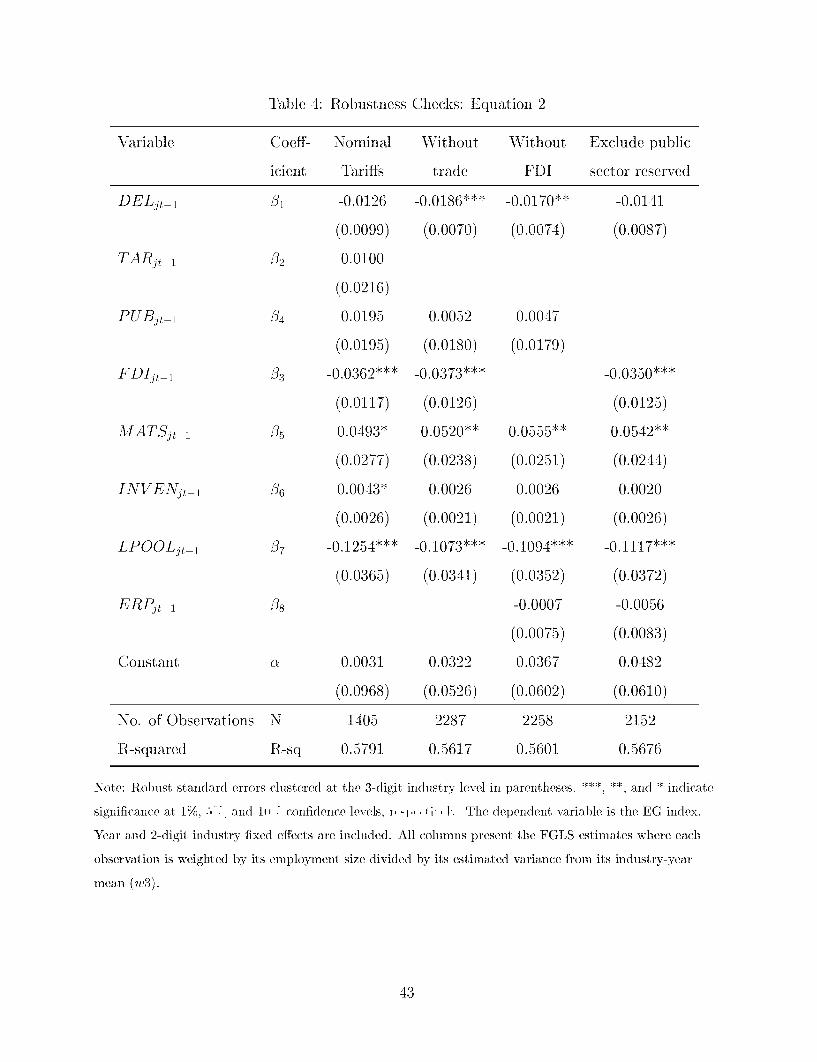
Table 4: Robustness Checks: Equation 2

Variable Coeff- Nominal Without Without Exclude public

icient Tariffs trade FDI sector reserved

DEL - 0 -0.0126 -0.0186*** -0.0170** -0.0141

(0.0099) (0.0070) (0.0074) (0.0087)

TARj 2 0.0100

(0.0216)

PUB 04 0.0195 0.0052 0.0047

(0.0195) (0.0180) (0.0179)

FDI 03 -0.0362*** -0.0373*** -0.0350***

(0.0117) (0.0126) (0.0125)

MATS- 05 0.0493* 0.0520** 0.0555** 0.0542**

(0.0277) (0.0238) (0.0251) (0.0244)

INVENj 06 0.0043* 0.0026 0.0026 0.0020

(0.0026) (0.0021) (0.0021) (0.0026)

LPOOL 07 -0.1254*** -0.1073*** -0.1094*** -0.1117***

(0.0365) (0.0341) (0.0352) (0.0372)

ERPt- 1 8 -0.0007 -0.0056

(0.0075) (0.0083)

Constant a 0.0031 0.0322 0.0367 0.0482

(0.0968) (0.0526) (0.0602) (0.0610)

No. of Observations N 1405 2287 2258 2152

R-squared R-sq 0.5791 0.5617 0.5601 0.5676

Note: Robust standard errors clustered at the 3-digit industry level in parentheses. **, and * indicate

significance at 1%,. and 1i'' confidence levels, 1. - Ii- 1-. The dependent variable is the EG index.

Year and 2-digit industry fixed effects are included. All columns present the FGLS estimates where each

observation is weighted by its employment size divided by its estimated variance from its industry-year

mean (w3).

43

Table 5: Estimation Results: Equations 3 and 5

Variable Coefficient Small Medium Large Pooled

plants sized plants plants model

DELt-1 01 -0.0241** 0.0196** 0.0358 -0.0446*

(0.0120) (0.0098) (0.0221) (0.0228)

ERPjt i 02 -0.0329** -0.0018 0.0552** -0.0595*

(0.0132) (0.0094) (0.0214) (0.0343)

PUBjt-I 04 -0.0275 -0.0137 0.0489* 0.0276

(0.0378) (0.0182) (0.0272) (0.0753)

FDIjtI 03 -0.0530** -0.0091 0.0241 -0.1262**

(0.0247) (0.0099) (0.0221) (0.0495)

MATS, 05 0.0689 -0.0073 -0.0426 0.0125

(0.0438) (0.0190) (0.0453) (0.0410)

INVENkt 06 0.0105 0.0053** -0.0026 0.0008

(0.0068) (0.0026) (0.0037) (0.0031)

LPOOL k 07 -0.1596*** 0.0102 -0.0469 -0.1549***

(0.0512) (0.0207) (0.0407) (0.0472)

D2jt 002 -0.2588

(0.1610)

D3jt /03 -0.5526***

(0.1684)

DELjt- 1 '12 0.0601**

*D2jt (0.0243)

DELjt- 1 713 0.0785**

*D3jt (0.0336)

ERPjti 1 '722 0.0565

*D2jt (0.0360)

continued on next page

44

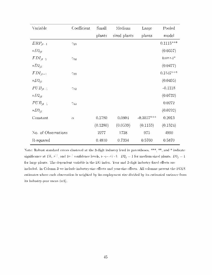
Variable Coefficient Small Medium Large Pooled

plants sized plants plants model

ERPjti 1 723 0.1115***

*D3jt (0.0357)

FDIjt-1 7 32 0 1""-

*D2jt (0.0477)

FDIjt-1 7 33 0.1547***

*D3jt (0.0495)

PUBi-1 42 -0.1118

*D2jt (0.0732)

PUBi-1 N43 0.0272

*D3jt (0.0792)

Constant a 0.1780 0.0804 -0.3057*** 0.2013

(0.1280) (0.0539) (0.1153) (0.1524)

No. of Observations 2277 1738 975 4990

R-squared 0.4810 0.7334 0.5760 0.5870

Note: Robust standard errors clustered at the 3-digit industry level in parentheses. ***, **, and * indicate

significance at 1%,. and i0' confidence levels, 1. - Ii- , 1. D2j = 1 for medium-sized plants. D3j = 1

for large plants. The dependent variable is the EG index. Year and 2-digit industry fixed effects are

included. In Column 3 we include industry-size effects and year-size effects. All columns present the FGLS

estimates where each observation is weighted by its employment size divided by its estimated variance from

its industry-year mean (w3).

45

Table 6: Hypothesis Tests: Equation 5 with size varying regressors

Hypothesis Estimate S.E. p-value

1 -0.04458 0.022823 0.052335

'12 0.060079 0.024273 0.01426

713 0.078459 0.033591 0.020628

'12 - '13 -0.01838 0.022744 0.-42I111".1

S1 + 12 0.015495 0.013-l-, 0.252193

S1 + 713 0.033875 0.022307 0.130654

2 -005953 0.034257 0.084

22 0.056532 0.035985 0.117975

723 0.111452 0.035743 0.002125

722 - 23 -0 -,.- 0.024546 0.026505

02 + 7'22 -0.003 0.020126 0.881769

02 23 0.051922 0.021908 0.018862

4 0.027566 0.075301 0.71475

Y42 -0.11182 0.073164 0.128201

Y43 0.027205 0.07916 0.731497

Y42 - 43 -0.13903 0.056185 0.01-121,

04 + -Y42 -0. I1-4't. 0.046049 0.068971

04 + Y43 0.054771 0.032085 (.,' '

03 -0.12615 0.049491 0.011651

Y32 0 -1 -11-'I l 0.04766 0.065279

Y33 0.154717 0.049507 0.002077

Y32 - 733 -0.06631 (.111-''1'2T 0.023054

33 + Y32 -0.03775 0.018933 0.047687

33 +7-33 (--i.'i t.u' 0.02137 0.183075

46

A Appendix I: Indian industrial policy and geographic

dispersion of industry

Mlarathe (1989) provides an in depth assessment of the objectives of the government and the

way industrial policy was used to affect the dispersion of Indian industry. At the time of

independence, manufacturing industry was highly localized. For example, out of 144 cotton

mills, 100 were located in one district. The government was concerned about regional con-

centration of employment and income, as well as about social and economic costs associated

with congestion. Further it was felt that 'new' enterprises may not choose their locations

optimally since they might be guided by linguistic/Iregional preferences and political pres-

sures. The government conceded that particularly in the early stages of development, access

to infrastructure may increase rjI1frni:if1j near urban areas (and that this was not neces-

sarily a bad thing) and that even highly planned economies like the USSR had substantial

variation in industrial distribution. But the Industrial Policy statements of 1945 and 1956

explicitly stated that a goal of industrial policy was to reduce concentration and/or develop

industry in a list of "Industrially Backward States".

Marathe (1989) states that during the first 20 years (1950-70), the central government

mainly used the distribution of public investment to try to affect the distribution of industry.

More backward states (those with lower shares of employment in manufacturing and/or low

per capita income) were assigned more investment. It was only in the 1970s that subsidy and

concessional finance schemes started being used. Further, even within the backward states,

some districts/areas were identified and even greater incentives were provided to locate in

these areas. As a result there was a rise in the share of industry located in backward states

but even within these states, there was an emergence of industrial areas near to already

relatively developed industrial centers. Further, most of the concessional schemes significantly

influenced the pattern of development of small enterprises, but not necessarily that of larger

enterprises. From the 1970s onwards, the government also disproportionately located public

sector enterprises in backward areas. In 1979, the share of industrially backward states in

the output (employment) of centrally owned public enterprises was 61%(5: ). But it is

important to note that most of these figures are accounted for by states (which happen to

47

be backward) with steel and coal mining operations.

The 1970s also saw the explicit use of the licensing regime as an important instrument for

determining location decisions by giving positive weight to license applications that located

new projects in backward areas. In the 1980s, the government streamlined and rationalized

the subsidy and concessional finance schemes (offered by both the central and state govern-

ments). Further, they divided the country into three types of districts (based on presence

of manufacturing industry), each with different amounts of subsidies and concessions. Other

than stating that -: of subsidy/ concession would be available if the project was located

in area y, the exact choice was up to the entrepreneur. This discretion opened the door to

the use of the licensing regime to locate industry in 'politically' popular areas. There were

instances where the approval of the license was delayed until the entrepreneur was willing to

move the location of the product to a backward district. In effect, since the licensing regime

was being used explicitly to direct new investment to certain geographic areas it is important

to analyze the long term effects, if any, of licensing.

48

B Appendix II: Supplementary Tables and Figures

---- -- -----

1980 1985 1990 1995 2000Yea

----- Sample sector ..... Census sector

-Total

Figure B.1: Annual number of observations in ASI data

0

. * --

1980 1985 1990 1995 2000Yen

SampleMean -------- CensusMeanSmrple S D - Census S D

Figure B.2: Annual Average Employment and its Standard DeviationNote: All averages are weighted by industry size (employment)

49

Table B.1: Annual Averages of Key Variables

Year EG Index MATSt INVENjt LPOOLte IRS 3 t DELjt PUBjt ERPjt FDIt

1980 0.10 0.57 -0.01 -0'.2s 2.64 0.00 0.33 90.36 0

1981 0.12 0.58 0.01 2371.42 2.54 0.00 0.31 90.45 0

1982 0.12 0.57 0.02 2566.29 3.31 0.00 0.30 91.28 0

1983 0.11 0.57 0.01 2636.69 2.97 0.00 0.31 91.63 0

1984 0.10 0.59 0.00 2954.33 3.17 0.19 0.33 93.96 0

1985 0.11 0.61 0.01 3248.50 2.78 0.23 0.32 93.24 0

1986 0.12 0.59 0.01 3382.43 2.71 0.27 0.32 101.02 0

1987 0.12 0.60 0.01 3517.64 2.38 0.31 0.32 101.71 0

l' 1 0.12 0.61 0.02 3915.60 2.71 0.31 0.32 101.26 0

1989 0.13 0.61 0.01 4237.95 2.77 0.28 0.25 103.58 0

1990 0.12 0.61 0.01 4616.20 3.11 0.29 0.25 104.53 0

1991 0.13 0.61 0.01 4450.14 2.87 0.96 0.24 60.79 0

1992 0.13 0.61 0.02 4646.35 3.25 0.96 0.22 61.40 0.22

1993 0.13 0.59 0.01 4872.91 3.35 0.97 0.18 61.30 0.22

1994 0.14 0.60 0.01 5217.37 3.81 0.97 0.15 61.48 0.22

1996 0.14 0.73 0.01 5979.65 4.32 0.99 0.15 32.21 0.23

1997 0.09 0.60 0.01 5688.28 4.17 0.99 0.17 35.31 0.19

1998 0.08 0.58 0.00 12546.07 4.13 0.73 0.14 34.09 0.20

1999 0.10 0.59 0.01 16753.86 3.97 0.99 0.13 32.03 0.24

Note: All averages are weighted by industry size (employment). The definition of the variables are as

follows. MATS3t = Materials per Rs. Sales; INVENjt = Inventories per Rs. Sales; LPOOLjt = Rs. sales

per employee; IRSP = Real capital per plant ('00000 Rupees); DELjt = Proportion of Output De-licensed;

PUBjt = Proportion of Output under Public Sector; ERPjt = Effective Rate of protection; FDIde =

Proportion of Output FDI 1l.. .I

50

Table B.2: 1i-t, Geographically Concentrated Industries in 1980

NIC Description EG Rank in Rank in Rank in Rank in

1980 1990 1994 1999318 Manufacture of coke oven products 1.044525 1 1 1 3229 Manufacture of pan masala, catechu 0.772687 2 20 26 62

and chewing lime325 Manufacture of mica products 0.7''''5 3 2 11 167225 Preparation of raw tobacco 0.724786 4 6 4 8307 Manufacture of matches 0.640719 5 3 3 155254 Spinning, weaving and finishing 0.608692 6 5 2 166

of jute and mesta textiles215 Processing of edible nuts 0.560939 7 10 9 67214 Coffee curing, i. . 0.47''S 8 12 14 7

grinding and blending385 Manufacture of sports 0.468759 9 39 34 43

and athletic goods213 Processing and blending of tea 0.434877 10 11 13 26

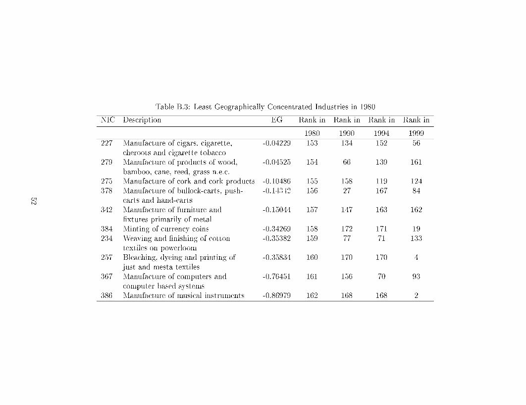
Table B.3: Least Geographically Concentrated Industries in 1980

NIC Description EG Rank in Rank in Rank in Rank in

1980 1990 1994 1999227 Manufacture of cigars, cigarette, -0.04229 153 134 152 56

cheroots and cigarette tobacco279 Manufacture of products of wood, -0.04525 154 66 139 161

bamboo, cane, reed, grass n.e.c.275 Manufacture of cork and cork products -0.10486 155 158 119 124378 Manufacture of bullock-carts, push- -0.1,1 12 156 27 167 84

carts and hand-carts342 Manufacture of furniture and -0.15044 157 147 163 162

fixtures primarily of metal384 Minting of currency coins -0.34269 158 172 171 19234 Weaving and finishing of cotton -0.35382 159 77 71 133

textiles on powerloom257 Bleaching, dyeing and printing of -0.35834 160 170 170 4

just and mesta textiles367 Manufacture of computers and -0.76451 161 156 70 93

computer based systems386 Manufacture of musical instruments -0.86979 162 168 168 2

Table B.4: Correlation Lii i: for Key VariablesEG Index MATSts INVENte LPOOLjt IRSts DELjt PUBjt ERPjt FDIt

EG Index 1MATSit 0.040 1INVENjt 0.040 0.009 1LPOOLt -0.077 0.025 -0.022 1IRSit -0.059 0.047 -0.017 0.634 1DELjt -0.020 -0.007 -0.026 0.124 -0.020 1PUBjt -0.025 0.035 -0.046 0.293 0.184 0.347 1ERPjt -0.086 -0.003 0.022 -0.090 -0.011 -0.370 -0.347 1FDIjt -0.0563 0.0006 -0.0157 0.0331 -0.031 0.2185 -0.0368 -0.0892 1

Note: The definition of the variables are as follows. MATSjt = Materials per Rs. Sales; INVENjt = Inventories per Rs. Sales; LPOOLjt = Rs.sales per employee; IRSjt = Real capital per plant; DELjt = Proportion of Output De-licensed; PUBjt = Proportion of Output under PublicSector; ERPjt = Effective Rate of protection; FDIjt = Proportion of Output FDI liberalized.

Table B.5: Estimation Results for Equation 2 with various weights

Variable Wt = Ljt Weight = WI Weight = W2 Lag=2 Lag=3DELjt-k -0.0163 -0.0182** -0.0166 -0.0274*** -0.0248**

(0.0149) (0.0072) (0.0148) (0.0103) (0.0101)ERPjt-k -0.0174 -0.0008 -0.0195 0.0079 0.0081

(0.0166) (0.0069) (0.0180) (0.0096) (0.0100)FDIjt-k -0.0385* -0.0357** -0.0424** -0.0199 -0.0250

(0.0222) (0.0142) (0.0213) (0.0137) (0.0166)MATSjit-k 0.0927** 0.0613*** 0.0759 0.0669* 0.0631*

(0.0432) (0.0227) (0.0500) (0.0342) (0.0325)INVENjt-k 0.0096** 0.0029 0.0087* -0.0015 -0.0030

(0.0045) (0.0021) (0.0046) (0.0023) (0.0026)LPOOLjit-k -0.1913*** -0.1066*** -0.1981*** -0.0622*** -0.0601***

(0.0546) (0.0340) (0.0570) (0.0169) (0.0172)PUBjt-k -0.0118 0.0103 -0.0168 0.0017 0.0031

(0.0394) (0.0181) (0.0394) (0.0217) (0.0214)Constant 0.0476 0.0343 0.0-1-1.3 0.5972*** 0.5647***

(0.1028) (0.0556) (0.1109) (0.1549) (0.1560)No. of Observations 2258 2258 2258 2172 2052R-squared 0.5744 0.5276 0.6177 0.5479 0.5454Breusch-Pagan 8.61test StatisticWhite's test 1195Statistic

Note: Robust standard errors clustered at the 3-digit industry level in parentheses. * ** and * indicatesignificance at 1%,. and 1i'' confidence levels, 1, -1 .. I1- - I-. The dependent variable is the EG index.Year and 2-digit industry fixed effects are included. FGLS estimates where each observation is weighted by:its employment size are presented in Column 1, its employment size divided by its estimated variance fromthe industry-mean in Column 2; its employment size divided by its estimated variance from the annualmean in Column 3. Columns 4 and 5 present the FGLS estimates where each observation is weighted by itsemployment size divided by its estimated variance from the industry-year mean (w3).

54

Table B.6: Estimation Results: Differences Post 1991

Variable Coefficient 1980-90 1991-99 Pooled

model

DEL t-1 01 -0.0170** 0.0141* -0.0185

(0.0077) (0.11r- -1) (0.0172)

ERPjt-i 02 0.0045 0.0009 -0.0086

(0.0072) (0.0074) (0.0125)

PUBj- 04 -0.0042 0.0233 -0.0077

(0.0176) (0.0200) (0.0391)

MATSJt- 05 0.0575** 0.0580** 0.0727

(0.0249) (0.0260) (0.0531)

INVENjt-I 06 -0.0002 0.0039 0.0066

(0.0019) (0.0026) (0.0060)

LPOOLjtl 07 -0.1268*** -0.1274*** -0.1766**

(0.0422) (0.0368) (0.0693)

D2t 002 -0.0409

(0.0660)

DELjt-l 712 0.0276

*D2jt (0.0217)

MATSji- 1 752 0.0311

*D2jt (0.0461)

INVENjt- 1 -Y62 0.0027

*D2jt (0.0074)

LPOOLjt- 1 '772 -0.0358

*D2jt (0.0378)

Constant -0.0102 0.0066 0.0144

(0.0556) (0.0618) (0.1168)

continued on next page

33

Variable Coefficient 1980-90 1991-99 Pooled

model

Observations 1247 1011 2258

R-squared 0.7346 0.5502 0.5752

Note: Robust standard errors clustered at the 3-digit industry level in parentheses. ***, **, and * indicate

significance at 1%,. and 1i'' confidence levels, 1. -1..- Ii- -1-. D2t 1 if year,>1990. The dependent

variable is the EG index. 2-digit industry fixed effects are included. All columns present the FGLS

estimates where each observation is weighted by its employment size divided by its estimated variance from

its industry-year mean (w3).

56

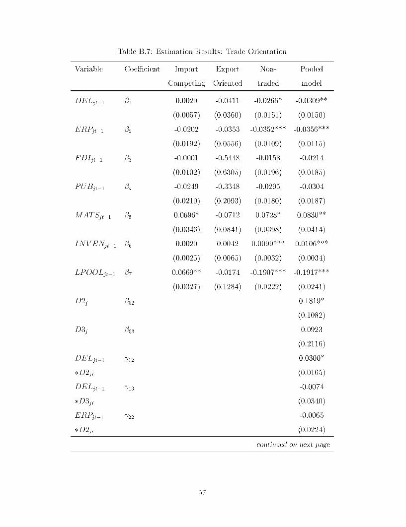
Table B.7: Estimation Results: Trade Orientation

Variable Coefficient Import Export Non- Pooled

Competing Oriented traded model

DEL - 0 0.0020 -0.0411 -0.0266* -0.0309**

(0.0057) (0.0360) (0.0151) (0.0150)

ERPjt-i 02 -0.0202 -0.0353 -0.0352*** -0.0356***

(0.0192) (0.0556) (0.0109) (0.0115)

FDI 03 -0.0001 -0.5448 -0.0158 -0.0214

(0.0102) (0.6305) (0.0196) (0.0185)

PUB 04 -0.0249 -0.3348 -0.0295 -0.0304

(0.0210) (0.2093) (0.0180) (0.0187)

MATSt-j 05 0.0696* -0.0712 0.0728* 0.0830**

(0.0346) (0.0841) (0.0398) (0.0414)

INVENjt-, 06 0.0020 0.0042 0.0099*** 0.0106***

(0.0025) (0.0065) (0.0032) (0.0034)

LPOOLjt-j 07 0.0669** -0.0174 -0.1907*** -0.1917***

(0.0327) (0.1284) (0.0222) (0.0241)

D2j 002 0.1819*

(0.1082)

D3j 003 0.0923

(0.2116)

DELjt-1 '12 0.0300*

*D2jt (0.0165)

DELjt- 1 713 -0.0074

*D3jt (0.0340)

ERPji '722 -0.0065

*D2jt (0.0224)

continued on next page

37

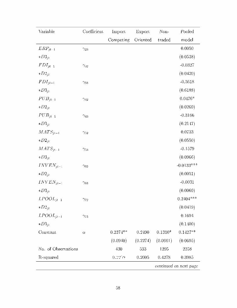
Variable Coefficient Import Export Non- Pooled

Competing Oriented traded model

ERPjti 1 723 0.0050

*D3jt (0.0538)

FDIji-1 'Y32 -0.0327

*D2jt (0.0420)

FDIji-1 7Y33 -0.5618

*D3jt (0.6188)

PUBjt-1 '42 0.0476*

*D2jt (0.0269)

PUBjt-1 'Y43 -0.3166

*D3jt (0.2147)

MATSi- 1 752 0.0733

*D2jt (0.0550)

MATSi- 1 753 -0.1579

*D3jt (0.0966)

INVENjt- 1 Y62 -0.0133***

*D2jt (0.0051)

INVENji- 1 Y63 -0.0031

*D3jt (0.0069)

LPOOLjt-1 '72 0.2404***

*D2jt (0.0419)

LPOOLjt-1 7 73 0.1694

*D3jt (0.1400)

Constant a 0.2374** 0.2490 0.1310* 0.1427**

(0.0940) (0.2274) (0.0661) (0.0695)

No. of Observations 430 533 1295 2258

R-squared 0. 0.2005 0.4278 0.3985

continued on next page

58

Variable Coefficient Import Export Non- Pooled

Competing Oriented traded model

Note: Robust standard errors clustered at the 3-digit industry level in parentheses. ***, **, and * indicate

significance at 1%,. and 1i'' confidence levels, 1. -1..- Ii- - 1-. D2 = 1 if industry is import-competing.

D3= 1 if industry is export-oriented. The dependent variable is the EG index. Year fixed effects are

included. All columns present the FGLS estimates where each observation is weighted by its employment

size divided by its estimated variance from its industry-year mean (w3).

Table B.8: Hypothesis Tests: Trade Orientation

Hypothesis Estimate S.E. p-value Hypothesis Estimate S.E. p-value

1 -0.031 0.015 0.041 05 0.083 0.041 0.046

712 0.030 0.016 0.071 752 0.073 0.055 0.185

713 -0.007 0.034 0.828 753 -0.158 0.097 0.104

-12 13 0.037 0.031 0.234 752 - 753 0.231 0.095 0.015

01 + 12 -0.001 0.007 0.897 05 + -5 0.156 0.036 0.00001 + 7'13 -0.038 0.031 0.212 05 + -5 -0.075 0.087 0.392

2 -0.036 0.011 0.002 06 0.011 0.003 0.002

722 -0.006 0.022 0.774 62 -0.013 0.005 0.010

723 0.005 0.054 0.926 63 -0.003 0.007 0.652

-22 -23 -0.011 0.056 0.838 62 -63 -0.010 0.007 0.156

02 + 7'22 -0.042 0.019 0.031 06 + 7Y62 -0.003 0.004 0.48902 + 7'23 -0.031 0.053 0.561 06 Y63 0.008 0.006 0.21404 -0.030 0.019 0.107 07 -0.192 0.024 0.000

Y42 0.048 0.027 0.078 '772 0.240 0.042 0.000

Y43 -0.317 0.215 0.142 773 0.169 0.140 0.228

Y42 - 743 0.364 0.215 0.092 772 - 773 0.071 0.142 0.618

04 + -Y42 0.017 0.019 0.372 07 + 7'72 0.049 0.034 0.15744 43 -0.347 0.214 0.106 07 + 7 -0.022 0.138 0.872

03 -0.021 0.018 0.248

Y32 -0.033 0.042 0.437

Y33 -0.562 0.619 0.365

Y32 - 733 0.529 0.620 0.394

03 +±Y32 -0.054 0.038 0.153

33 + Y33 -0.583 0.619 0.347

59