To what extent are unstable the maxima of thepotential?

Antonio J. Urena

July 5, 2017

Abstract. The classical Lagrange-Dirichlet stability theorem states that, fornatural mechanical systems, the strict minima of the potential are dynamicallystable. Its converse, i.e., the instability of the maxima of the potential, hasbeen proved by several authors including Liapunov (1892), Hagedorn (1971),or Taliaferro (1980), in various degrees of generality. We complement theirtheorems by presenting an example of a smooth potential on the plane havinga maximum and such that the associated dynamical system has a convergingsequence of periodic orbits. This implies that the maximum is not unstablein a stronger sense considered by Siegel and Moser.

1 Introduction

Consider the Newtonian system of equations

q = −∇V (q) , q ∈ Rd , (1)

where V : Rd → R is a given potential having a local maximum at some pointq∗ ∈ Rd. In his 1892 PhD dissertation [5], Liapunov showed that if this maximumis nondegenerate, then the corresponding equilibrium is dynamically unstable. Li-apunov’s instability theorem was extended by Hagedorn [2], who used variationalmethods to prove the instability of all isolated maxima of the potential, and Talia-ferro [8], who removed the isolatedness assumption from Hagedorn’s theorem. Re-sults of this type have been named as converses of the Lagrange-Dirichlet stabilitytheorem, and the associated literature is very ample, see for instance [3, 6].

In the above-mentioned papers, the word instability is understood as the logicalnegation of Liapunov stability. In particular, it means at the same time past andfuture instability, two concepts which are equivalent in the Hamiltonian framework.However, a stronger notion of instability was considered by Siegel and Moser in [7,§25]. According to their definition, the equilibrium q∗ ∈ Rd is unstable if thereis a neighborhood N of (q∗, 0) in the phase space such that every globally-definedsolution q : R → Rd of (1), q(t) 6≡ q∗, satisfies (q(tq), q(tq)) 6∈ N for some tq ∈ R.In other words, (q∗, 0) is the maximal subset of N which invariant by the flow.Observe, for instance, that a hyperbolic fixed point is always unstable in this strongersense, whereas a nonisolated fixed point never is.

1

The question which motivates this paper is the following: assume that the po-tential V attains its maximum at q∗ ∈ RN , and that this maximum is isolated as acritical point of V , does it imply that q∗ is unstable in the stronger sense of Siegeland Moser?

The answer to this question is affirmative in the 1-dimensional case d = 1,as an easy conservation-of-energy argument shows. It is also affirmative if oneassumes that the Hessian matrix of the (sufficiently smooth) potential V is negativesemidefinite on some neighborhood of q∗; indeed, under this assumption, the functiont 7→ −V (q(t)) is convex as long as q(t) belongs to the neighborhood, as one promptlychecks. However, this question turns out to be false in general. The goal of thispaper is to prove the following:

Theorem 1.1. There exists a C∞ function V : R2 → R satisfying:

(a) V (0) = maxR2 V ,

(b) ∇V (q) 6= 0 for any q 6= 0 ,

(c) there exists a sequence Tn > 0 of positive numbers and a sequence qn : R/TnZ→R2 of nontrivial periodic solutions of q = −∇V (q) such that

maxt∈R

(‖qn(t)‖+ ‖qn(t)‖)→ 0 as n→ +∞ .

We do not know whether such an example exists in the analytic case. In ourconstruction, the sequence of periods Tn is divergent.

2 Admissible closed curves and potentials

A key advance towards the proof of Theorem 1.1 will consist in building a closed,simple and nonconvex curve L in the plane, and a potential U with a non-vanishinggradient which points inwards on the concave section of L and outwards on the con-vex part. This construction, which will be formulated more precisely in Proposition2.1, will occupy us through Sections 2 and 3.

The closed curve L will be defined by some 2π-periodic parametrization ` = `(t).For simplicity reasons, we shall further impose some symmetry conditions on ourproblem; thus, from now on we denote by S to the symmetry in R2 with respect tothe y axis, i.e., S(x, y) := (−x, y).

It will be convenient to introduce some definitions here. The parameterizedclosed curve ` : R/2πZ→ R2, ` = `(t) will be termed admissible provided that it isC∞, simple, and satisfies:

(`i) `(−t) = S(`(t)) ∀t ∈ R/2πZ ,

(`ii) `(R/2πZ) ⊂]− 1, 1[2, `(]0, π[) ⊂]0,+∞[×R ,

(`iii) ˙(t) 6= 0 ∀t ∈ R/2πZ ,

2

and, for some t∗ ∈]0, π/2[,

(`iv) det( ˙(t), ¨(t))

< 0 if 0 ≤ t < t∗

> 0 if t∗ < t ≤ π,

d

dt

∣∣∣t=t∗

det( ˙(t), ¨(t)) > 0 .

On the other hand, the function U : R2 → R, U = U(x, y), will be said to be anadmissible potential provided that it is C∞ and satisfies

(Ui): U(x+ 2, y) = U(−x, y) = U(x, y);

(Uii): U(x, y) = y if |y| ≥ 1;

(Uiii): ∇U(x, y) 6= 0 ∀(x, y) ∈ R2 .

Finally, the admissible closed curve ` and the admissible potential U will becalled coupled provided that

(U`i): 〈∇U(`(t)), ˙(t)〉 > 0 ∀t ∈]0, π[ ,d2

dt2

∣∣∣t=0U(`(t)) > 0 >

d2

dt2

∣∣∣t=π

U(`(t)) ,

(U`ii): det(∇U(`(t)), ˙(t))

< 0 if 0 ≤ t < t∗

> 0 if t∗ < t ≤ π,

d

dt

∣∣∣t=t∗

det(∇U(`(t)), ˙(t)) > 0,

where t∗ is the same number appearing in assumption (`iv). If only (U`i) is ensuredwe shall say that ` and U are semicoupled.

We can interpret (`iv) in the sense that the curvature of the closed curve L :=`(R/2πZ) changes sign at `(t∗). Similarly, (U`ii) states that the restriction of ∇Uto L goes from pointing inwards to pointing outwards at the same point.

Our first task in this paper, announced at the beginning of this section, willconsist in checking that the definitions above are not empty:

Proposition 2.1. There exist an admissible closed curve ` and an admissible po-tential U which are coupled.

The proof of Proposition 2.1 will be divided into three steps:

• Firstly, we shall present a family `λλ of admissible closed curves.

• Secondly, we shall describe an admissible potential U which is semicoupled tosome curves of this family.

• Finally, we shall modify U so that it becomes coupled to one of these admissibleclosed curves. This last step will be carried out in the next section.

Concerning the first step, the curves which we have in mind are called limaconsof Pascal1 and have been known in geometry and the arts for centuries [1]. In polarcoordinates (ϑ, %), they are defined by the implicit equation

Lλ : % =1

4(λ+ sinϑ) .

1The French word ‘limacon’ can be translated as ‘snail’.

3

Here, 1 < λ ≤ 2 is a parameter. Notice that all these closed curves are smoothand simple. For λ = 2 the corresponding curve is convex, but we will be mostlyinterested in the case λ ∈]1, 2[, for which the curvature changes sign. See Fig. 1.The choice of the scaling coefficient 1/4 has been made so that these curves fit insidethe open square ]− 1, 1[×]− 1, 1[, as required by condition (`ii). Notice finally thatour curves are symmetric with respect to the ordinate axis, i.e. S(Lλ) = Lλ.

-0.3 0.3

-0.1

0.4

L1.1

-0.4 0.4-0.1

0.5

L1.5

-0.4 0.4

-0.2

0.6

L2

Figure 1: Pascal’s limacons for three possible values of the parameter.

One can parameterize these curves as follows:

`λ : R/2πZ→ Lλ , `λ(t) :=1

4(λ− cos t)

(sin t− cos t

).

For 1 < λ < 2, the parametrization `λ crosses a curvature-changing point of Lλ at

tλ = arccos

(λ2 + 2

3λ

)∈]0, π/2[. One easily arrives to the following result:

Lemma 2.2. The closed curves `λ are admissible for every λ ∈]1, 2[.

This completes the first step of the proof of Proposition 2.1, so that we turn nowour attention to the second step. To this respect one has the following:

Lemma 2.3. There exists an admissible potential U : R2 → R, U = U(x, y) with

(Uiii): ∂U/∂y > 0 on R2,

which is semicoupled with `λ provided that λ ∈]1, 2[ is close enough to 2.

Proof. Choose some cutoff function m ∈ C∞(R) with

m(u) = 0 if u 6∈ [−1, 0] , m(u) > 0 if u ∈]− 1, 0[ , |m′(u)| < 1 ∀u ∈ R ,

and consider the function U : R2 → R defined by

U(x, u+m(u) cos(πx)) = u , (x, u) ∈ R2 . (2)

One easily checks properties (Ui),(Uii),(Uiii). In addition, (U`i) follows fromdirect computations for `2, and from a continuity argument for `λ with λ close to 2,see Fig. 2. The proof is complete.

4

Figure 2: Some of the level curves of the potential U of Lemma 2.3 together withL2 (left picture), and Lλ with λ ∈]1, 2[ close to 2 (right picture).

3 Bending the level curves of the potential

We are now ready to embark on the third and final step of the proof of Proposition2.1. With this goal, our starting point will consist in choosing some admissible closedcurve ` := `λ and some semicoupled admissible potential U as given by Lemma 2.3.We shall leave ` untouched; thus, in order to ensure (U`ii) some modifications on

the potential are needed. The main idea consists in modifying the level curves of Uin a neighborhood K of `(t∗); we give the details below.

The end of the proof of Proposition 2.1. Let J =

(0 1−1 0

)be the 90 rotation in

the clockwise sense, and let the vector field Z : R2 → R be defined by Z := J∇U .The integral trajectories of Z travel along the level curves of U from left to right, andwe shall parametrize them simultaneously by means of the map ψ : R2 → R2, ψ =ψ(s, η), defined by the initial value problem

∂ψ

∂s(s, η) = Z(ψ(s, η)) , ψ(0, η) = (0, η) .

One checks that ψ : R2 → R2 is an orientation-preserving diffeomorphism ofclass C∞. It satisfies

ψ(−s, η) = S(ψ(s, η)) , ψ(s, η) = s if |η| ≥ 1 , ψ(s+ P (η), η) = ψ(s, η) + (2, 0) ,(3)

for some smooth function P : R→]0,+∞[ with P (η) = 2 if |η| ≥ 1.

We further observe that, setting L := `(R/2πZ),

ψ(R× η) ∩L 6= ∅ ⇐⇒ η ∈ [η−, η+] ,

where η− < η+ are the ordinate components of `(0) and `(π) respectively. Moreover,for η ∈]η−, η+[ the set ψ(R×η)∩L ∩ (]0,+∞[×R) is a singleton. This fact leadsus to consider the set

Ω := ψ(s, η) : s ∈ R , η− < η < η+ = ω ∈ R2 : U(`(0)) < U(ω) < U(`(π)) ,

5

and the functions S ,H , σ : Ω→ R defined by

ψ(S (ω),H (ω)) = ω , ψ(σ(ω),H (ω)) ∈ L ∩ (]0,+∞[×R) , ω ∈ Ω .

We notice that

∇(S − σ)(`(t)) =1

〈∇U(`(t)), ˙(t)〉J ˙(t) , t ∈]0, π[ ,

as one can easily check by multiplying both sides of the equality by ˙(t) and Z( ˙(t)).We deduce that

〈Z(`(t)),∇(S − σ)(`(t))〉 > 0 , 〈J ˙(t),∇(S − σ)(`(t))〉 > 0 , t ∈]0, π[ , (4)

two inequalities which will play a role later. On the other hand, it follows from thecombination of assumptions (Ui) and (Uiii) that both ∇U(`(0)) and ∇U(`(π)) arepositive multiples of (0, 1), while (`i), (`ii) and (`iii) together imply that both ˙(0)and − ˙(π) are positive multiples of (1, 0). Hence,

〈Z(`(0)), ˙(0)〉 > 0 > 〈Z(`(π)), ˙(π)〉 ,

and, by continuity, it is possible to find some 0 < ε < t∗/2 such that〈Z(`(t)), ˙(t)〉 > 0 ∀t ∈ [0, 2ε]

〈Z(`(t)), ˙(t)〉 < 0 ∀t ∈ [π − 2ε, π]. (5)

Combining (`ii) and (4) one can find some constant δ > 0 small enough so thatthe compact set

K :=ω ∈ Ω : H (`(ε)) ≤H (ω) ≤H (`(π − ε)), |(S − σ)(ω)| ≤ δ

,

satisfies the following properties:

(K1) K ⊂]0, 1[×]− 1, 1[ ,

(K2) 〈Z(ω),∇(S − σ)(ω)〉 > 0 ∀ω ∈ K,

(K3) there exist c > 0 and a C∞ vector field Z : K → R2 withZ(`(t)) = J ˙(t)− c(t− t∗) ˙(t) ∀t ∈ [ε, π − ε]〈Z(ω),∇(S − σ)(ω)〉 > 0 ∀ω ∈ K

.

Fix now some cutoff function m ∈ C∞(R2) satisfying

0 ≤ m ≤ 1 on R2 , m ≡ 0 on R2\K , m(`(t)) = 1 ∀t ∈ [2ε, π − 2ε] ,

6

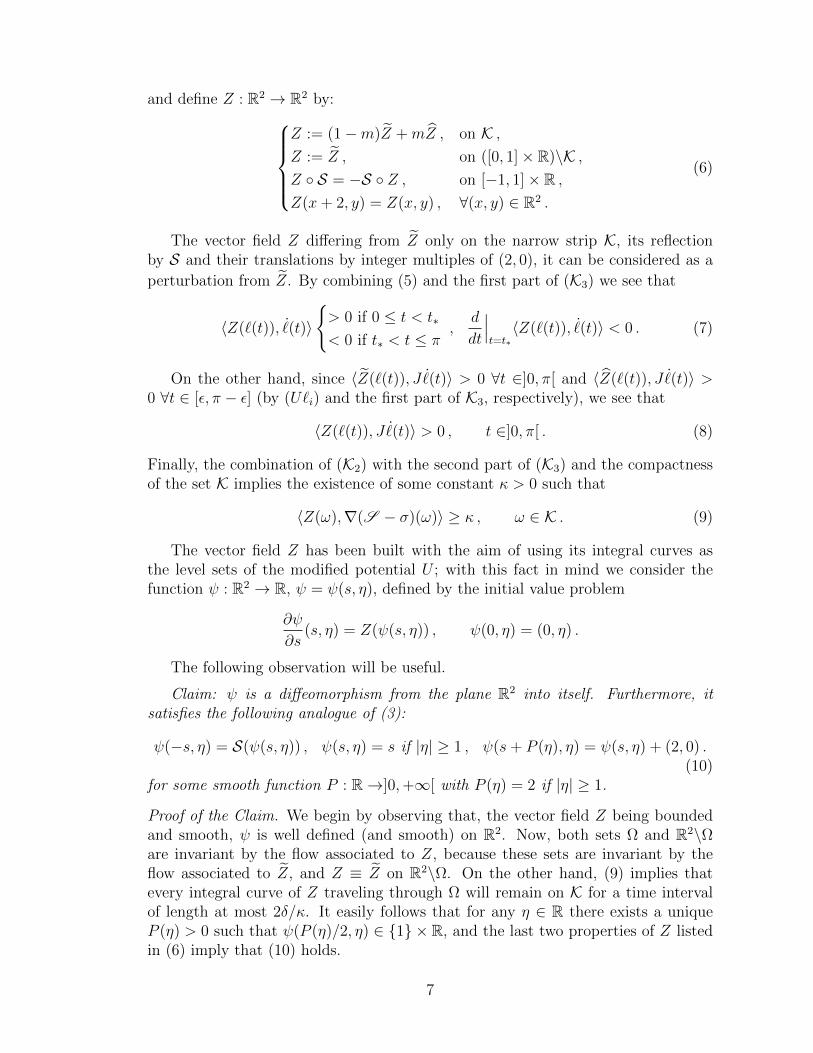
and define Z : R2 → R2 by:Z := (1−m)Z +mZ , on K ,Z := Z , on ([0, 1]× R)\K ,Z S = −S Z , on [−1, 1]× R ,Z(x+ 2, y) = Z(x, y) , ∀(x, y) ∈ R2 .

(6)

The vector field Z differing from Z only on the narrow strip K, its reflectionby S and their translations by integer multiples of (2, 0), it can be considered as a

perturbation from Z. By combining (5) and the first part of (K3) we see that

〈Z(`(t)), ˙(t)〉

> 0 if 0 ≤ t < t∗

< 0 if t∗ < t ≤ π,

d

dt

∣∣∣t=t∗〈Z(`(t)), ˙(t)〉 < 0 . (7)

On the other hand, since 〈Z(`(t)), J ˙(t)〉 > 0 ∀t ∈]0, π[ and 〈Z(`(t)), J ˙(t)〉 >0 ∀t ∈ [ε, π − ε] (by (U`i) and the first part of K3, respectively), we see that

〈Z(`(t)), J ˙(t)〉 > 0 , t ∈]0, π[ . (8)

Finally, the combination of (K2) with the second part of (K3) and the compactnessof the set K implies the existence of some constant κ > 0 such that

〈Z(ω),∇(S − σ)(ω)〉 ≥ κ , ω ∈ K . (9)

The vector field Z has been built with the aim of using its integral curves asthe level sets of the modified potential U ; with this fact in mind we consider thefunction ψ : R2 → R, ψ = ψ(s, η), defined by the initial value problem

∂ψ

∂s(s, η) = Z(ψ(s, η)) , ψ(0, η) = (0, η) .

The following observation will be useful.

Claim: ψ is a diffeomorphism from the plane R2 into itself. Furthermore, itsatisfies the following analogue of (3):

ψ(−s, η) = S(ψ(s, η)) , ψ(s, η) = s if |η| ≥ 1 , ψ(s+ P (η), η) = ψ(s, η) + (2, 0) .(10)

for some smooth function P : R→]0,+∞[ with P (η) = 2 if |η| ≥ 1.

Proof of the Claim. We begin by observing that, the vector field Z being boundedand smooth, ψ is well defined (and smooth) on R2. Now, both sets Ω and R2\Ωare invariant by the flow associated to Z, because these sets are invariant by theflow associated to Z, and Z ≡ Z on R2\Ω. On the other hand, (9) implies thatevery integral curve of Z traveling through Ω will remain on K for a time intervalof length at most 2δ/κ. It easily follows that for any η ∈ R there exists a uniqueP (η) > 0 such that ψ(P (η)/2, η) ∈ 1 × R, and the last two properties of Z listedin (6) imply that (10) holds.

7

In particular, all the integral curves ψ(·, η) of the vector field Z are periodicwhen projected on the cylinder (R/2Z) × R, but none of them is periodic whenregarded on the plane R2. It follows that the map ψ : R2 → R2, which is easily seento be a local diffeomorphism, is also injective. By combining the second and thirdstatements in (10) we deduce that

lim|(s,η)|→∞

〈ψ(s, η), (s, η)〉|(s, η)|

= +∞ ,

and a degree argument implies that ψ : R2 → R2 is surjective. In consequence, ψ isa diffeomorphism, proving the Claim.

To conclude the argumentation of Proposition 2.1, it suffices to define

U : R2 → R , U(ψ(s, η)) := U(0, η) , (11)

so that

∇U(ψ(s, η)) = −(∂U/∂η)(0, η)

det(ψ′(s, η))JZ(ψ(s, η)) . (12)

Now, the two parts of (Ui) follow, respectively, from the last and first parts of(10), while (Uii) is a consequence from the second part of (10) in combination with

(11) and the analogous assumptions satisfied by U . Moreover, (Uiii) arises from(12) and the fact that, by (9), the vector field Z does not vanish. Statement (U`i)follows from the combination of (8) and (12) (for its first part) and the analogous

assumption satisfied by U (in its second part). Finally, (U`ii) arises from (7)-(12).It completes the proof.

4 A conformally-Newtonian equation

From now on, we fix an admissible closed curve ` and a coupled admissible potentialU ; the existence such a pair is ensured by Proposition 2.1. The combination ofconditions (`i)-(Ui) on one hand, and (`iv)-(U`ii) on the other, implies that thefunction χ : R/2πZ→ R defined by

χ(t) :=det( ˙(t), ¨(t))

det(∇U(`(t)), ˙(t)), t ∈ (R/2πZ)\−t∗, t∗ ,

and extended to ±t∗ by continuity, is actually C∞-smooth, even and positive. Thisfact will be used in the proof of our next result.

Lemma 4.1. Under the above, there exist some T > 0, a C∞ diffeomorphismτ : R/TZ→ R/2πZ and a C∞ function w : R/TZ→ R such that

(i) τ(−t) = −τ(t), w(−t) = w(t) > 0 ∀t ∈ R/TZ ,

and, letting γ(t) := `(τ(t)), one has:

8

(ii) γ(t) = −w(t)∇U(γ(t)) ∀t ∈ R/TZ.

Proof. Differentiating twice in the equality γ(t) = `(τ(t)) we see that statement (ii)above is equivalent to

τ ˙(τ) + τ 2 ¨(τ) = −w∇U(`(τ)) ,

where, for simplicity, we have dropped the dependence on the time variable t fromthe notation. This equation in R2 can be equivalently rewritten as the system

τ | ˙(τ)|2 + τ 2〈¨(τ), ˙(τ)〉 = −w〈∇U(`(τ)), ˙(τ)〉τ 2 det(¨(τ), ˙(τ)) = −w det(∇U(`(τ)), ˙(τ))

,

or what is the same (isolating w in the second equation and replacing its value intothe first one),

τ /τ = −h(τ)τ

w = χ(τ) τ 2,

where h(τ) :=(〈¨(τ), ˙(τ)〉 + χ(τ)〈∇U(`(τ)), ˙(τ)〉

)/| ˙(τ)|2. Integration of the first

equation transforms the system above intoτ = ce−H(τ) for some constant c > 0

w = χ(τ) τ 2, (13)

where H(τ) :=

∫ τ

0

h(r)dr. Notice that h is 2π-periodic and odd, implying that H

is 2π-periodic and even.

We fix now an arbitrary number c > 0 (for instance, c = 1), and observe that thesolution τ = τ(t) of the first equation of (13) with τ(0) = 0 is an odd diffeomorphismfrom R into itself satisfying τ(t + T ) = τ(t) + 2π for T = τ−1(2π). We define was in the second equation of (13), and observe that (i)-(ii) hold. This proves thelemma.

5 From conformally-Newtonian to Newtonian

The following lemma could be taken from an elementary course of real analysis, andwe state it without proof.

Lemma 5.1. Let a > 0 be some positive number and u,w : [−a, a] → R be evenfunctions of class C∞. Assume that u(0) > 0 and u(t) > 0 ∀t ∈]0, a]. Then, thereexists a C∞ function f : R→ R such that w(t) = f(u(t)) for any t ∈ [−a, a].

Remark: Setting u+ := u∣∣]0,a]

:]0, a] →]u(0), u(a)], it is clear from the assump-

tions that f∣∣]u(0),u(a)]

= w u−1+ ∈ C∞(]u(0), u(a)]). Consequently, the interest of the

lemma is to ensure that the derivatives of all orders of f are continuous up to u(0).

9

From this moment on we shall work on the cylinder (R/2Z)×R with coordinates(θ, y), instead of the plane R2. Notice that, by assumption (Ui), one can actuallysee the potential U of Proposition 2.1 as being defined on this cylinder.

Corollary 5.2. There exists a C∞ potential W : (R/2Z) × R → R, W = W (θ, y),with

(W1) W (θ, y) ≡ 1 if y ≤ −1, W (θ, y) ≡ 0 if y ≥ 1 ,

(W2) ∇W (θ, y) 6= 0 if |y| < 1 ,

and, for some 0 < ε1 < 1 ,

(W3) (∂W/∂y)(θ, y) < 0 if 1− ε1 < |y| < 1 ,

and such that the equation γ = −∇W (γ) has a closed orbit

γ : R/TZ→]− 1, 1[2 .

Proof. Let U : (R/2Z)×R→ R and ` : R/2πZ→]−1, 1[2 be as given by Proposition2.1; let w : R→]0,+∞[ and γ := ` τ : R/TZ→ R2 be as given by Lemma 4.1, andset u(t) := U(γ(t)). This is an even function, both with respect to t = 0 and withrespect to t = T/2, and it follows from Lemma 5.1 that there exists a C∞ functionf : R→]0,+∞[ with w(t) = f(u(t)) = f(U(γ(t))) for any t. Set F (r) :=

∫ r−1 f(u)du

and choose some smooth function ϕ : R→ R with

(ϕ1) ϕ(r) ≡ 0 on ]−∞, 0] , ϕ(r) ≡ 1 on [F (1),+∞[ ,

(ϕ2) ϕ′(r) > 0 on ]0, F (1)[,

(ϕ3) ϕ′(r) ≡ ϕ∗ > 0 on[F (minγ(R) U), F (maxγ(R) U)

],

and define γ : R→]− 1, 1[2 and W : (R/2Z)× R→ R by

γ(t) := S(γ(√ϕ∗ t)) , W := ϕ F U S ,

where we denote by S : (R/2Z)×R→ (R/2Z)×R the symmetry S(θ, y) := (θ,−y).The result follows.

6 From the cylinder into a ring

It will be convenient to consider, for any ρ > 1, the open ring

Rρ := q ∈ R2 : ρ− 1 < |q| < ρ+ 1 .

We observe the following geometrical property: for each 0 < α < 1 there exists someρ(α) > 1 such that, for any ρ ≥ ρ(α), one has

[−α, α]× [ρ− α, ρ+ α] ⊂ Rρ . (14)

In these situations one can use the following

10

Lemma 6.1. Let 0 < α < 1 < ρ be such that (14) holds. Then, there exists a C∞

diffeomorphism Γ : (R/2Z) × [−1, 1] → Rρ with Γ((R/2Z) × ±1) = q ∈ R2 :|q| = ρ± 1 and

Γ(x, y) = (x, y + ρ) if (x, y) ∈ [−α, α]× [−α, α] .

This result is elementary and its proof will be skipped. It will play a role in theproof of the following

Proposition 6.2. There exists some ρ > 1 and a C∞ potential V : R2 → Rsatisfying:

(V1) V(q) = 1 if |q| ≤ ρ− 1, V(q) = 0 if |q| ≥ ρ+ 1 ,

(V2) ∇V(q) 6= 0 ∀q ∈ Rρ,

and, for some 0 < ε < 1,

(V3) 〈∇V(q), q〉 ≤ 0 if dist(q, ∂Rρ) < ε,

and such that the equation q = −∇V(q) has a closed orbit q : R/TZ→ Rρ.

Proof. Choose W : (R/2Z)×R→ R and γ : R/TZ→]−1, 1[2 as given by Corollary5.2. Pick some 0 < α < 1 such that γ(R) ⊂] − α, α[×] − α, α[, and fix ρ > 1 bigenough so that (14) holds. Choose Γ as in Lemma 6.1 and set

V : R2 → R , V(q) :=

W (Γ−1(q)) if q ∈ Rρ

1 if |q| ≤ ρ− 1

0 if |q| ≥ ρ+ 1

,

and q := Γ γ = (0, ρ) + γ. Now, it is clear that V and q are both C∞; furthermore,(V1), (V2) and (V3) follow, respectively, from (W1), (W2) and (W3). The proof iscomplete.

Remark. There is an alternative way to deduce Proposition 6.2 (for the ring ofradii e±π instead of Rρ) from Corollary 5.2 without any need of Lemma 6.1. Indeed,the complex exponential z 7→ eπz is a conformal map, and one can use an argumentdue to Goursat [4] to transform Newtonian equations on the cylinder into Newtonianequations on the ring. We have opted by the proof above because of its conceptualsimplicity.

We are now ready to prove the main result of this paper.

Proof of Theorem 1.1. Choose V : R2 → R, 0 < ε < 1 and q : R/TZ→ Rρ as givenby Proposition 6.2. For any nonnegative integer n we define

Mn := max

|∂αV(q)| : q ∈ R2

α = (α1, α2) ∈ Z2, αi ≥ 0, α1 + α2 ≤ n

.

11

Set µ := (ρ + 1)/(ρ − 1) > 1, and G :=⋃n≥0

]ρ+1−εµn+1 ,

ρ−1+εµn

[(the intervals are

nonempty and nonoverlapping). Choose some C∞ function h : [0,+∞[→ R with

h′(r) < 0 if r ∈ G , h′(r) = 0 if r ∈ [0,+∞[\G , (15)

and define V : R2 → R by:

V (q) := h(|q|) +∞∑n=0

(1

2nMn µn2

)V(µnq) , q ∈ R2 .

In this way, it is clear that V ∈ C∞(R2). It has a (degenerate) maximum atthe origin, which (by (V2)-(V3)-(15)) is the only critical point of V on q ∈ R2 :|q| ≤ ρ + 1. Finally, one checks that, setting Tn := 2n/2

√Mn µ

n2/2−n T , thenqn(t) := (1/µn)q(Tt/Tn) is a solution of q = −∇V (q) for each n. The proof iscomplete.

Compliance with Ethical Standards: The author declares that he has noconflict of interest.

Acknowledgements: I am grateful to R. Ortega for interesting discussions onthis paper, as well as pointing to me the connections to reference [4].

References

[1] Durer, A., Underweysung der Messung. Nuremberg, 1538.

[2] Hagedorn, P., Die Umkehrung der Stabilitatssatze von Lagrange-Dirichlet undRouth. Arch. Rational Mech. Anal. 42 (1971), 281-316.

[3] Hagedorn, P.; Mawhin, J., A simple variational approach to a converse of theLagrange-Dirichlet theorem. Arch. Rational Mech. Anal. 120 (1992), no. 4, 327–335.

[4] Goursat, E., Les transformations isogonales en Mecanique. C. R. Acad. Sci. Paris108 (1889), 446–448.

[5] Liapunov, A.M., The General Problem of Stability of Motion (in Russian). Doc-toral dissertation, University of Kharkov, Kharkov Mathematical Society, 1892.

[6] Negrini, P., On the inversion of Lagrange-Dirichlet theorem. Resenhas 2 (1995),no. 1, 83–114.

[7] Siegel, C.L.; Moser, J.K., Lectures on Celestial Mechanics. Classics in Mathe-matics. Springer-Verlag, Berlin, 1995.

[8] Taliaferro, S.D., An inversion of the Lagrange-Dirichlet stability theorem. Arch.Rational Mech. Anal. 73 (1980), no. 2, 183–190.

12