To my family and grandfather

List of papers

This thesis is based on the following papers, which are referred to in the textby their Roman numerals.

I Correlation-induced non-Abelian quantum holonomiesM. Johansson, M. Ericsson, K. Singh, E. Sjöqvist, and M. S.WilliamsonJ. Phys. A: Math Theor. 44 145301 (2011)

II Topological phases and multiqubit entanglementM. Johansson, M. Ericsson, K. Singh, E. Sjöqvist, and M. S.WilliamsonPhys. Rev. A 85 032112 (2012)

III Non-adiabatic holonomic quantum computationE. Sjöqvist, D. M. Tong, B. Hessmo, M. Johansson, and K. Singhpreprint: arXiv:1107.5127v2

IV Robustness of non-adiabatic holonomic gatesM. Johansson, E. Sjöqvist, L. M. Andersson, M. Ericsson, B. Hessmo,K. Singh, and D. M. Tongpreprint: arXiv:1204.5144v1

Reprints were made with permission from the publishers.

Other papers not included in the thesis arei Reverse Si=C Bond Polarization as a Means for Stabilization of Silaben-zenes: A Computational InvestigationA. M. El-Nahas, M. Johansson, and H. OttossonOrganometallics 22 5556 (2003)

ii Geometric local invariant and pure three-qubit statesM. S. Williamson, M. Ericsson, M. Johansson, E. Sjöqvist, A. Sudbery, V.Vedral, and W. K. WoottersPhys. Rev. A 83 062308 (2011)

iii Global asymmetry of many-qubit correlations: A lattice-gauge-theory ap-proachM. S. Williamson, M. Ericsson, M. Johansson, E. Sjöqvist, A. Sudbery,and V. VedralPhys. Rev. A 84 032302 (2011)

Contents

1 Introduction . . . . . . . . . . . . . . . . . . . . . . . . . . . . . . . . . . . . . . . . . . . . . . . . . . . . . . . . . . . . . . . . . . . . . . . . . . . . . . . . . . . . . . . . . . . . . . . . . . 91.1 Emergence of quantum mechanics . . . . . . . . . . . . . . . . . . . . . . . . . . . . . . . . . . . . . . . . . . . . . . . . . . 91.2 Quantum formalism . . . . . . . . . . . . . . . . . . . . . . . . . . . . . . . . . . . . . . . . . . . . . . . . . . . . . . . . . . . . . . . . . . . . . . . 11

1.2.1 The U(1)-bundle structure of Hilbert space . . . . . . . . . . . . . . . . . . . 121.3 Quantum information . . . . . . . . . . . . . . . . . . . . . . . . . . . . . . . . . . . . . . . . . . . . . . . . . . . . . . . . . . . . . . . . . . . . . 131.4 Conceptual foundations of quantum superposition . . . . . . . . . . . . . . . . . . . . . . 14

2 Quantum nonlocality . . . . . . . . . . . . . . . . . . . . . . . . . . . . . . . . . . . . . . . . . . . . . . . . . . . . . . . . . . . . . . . . . . . . . . . . . . . . . . . . . 172.1 Quantum interference . . . . . . . . . . . . . . . . . . . . . . . . . . . . . . . . . . . . . . . . . . . . . . . . . . . . . . . . . . . . . . . . . . . . 182.2 Entanglement . . . . . . . . . . . . . . . . . . . . . . . . . . . . . . . . . . . . . . . . . . . . . . . . . . . . . . . . . . . . . . . . . . . . . . . . . . . . . . . . . . 192.3 Characterizing entanglement . . . . . . . . . . . . . . . . . . . . . . . . . . . . . . . . . . . . . . . . . . . . . . . . . . . . . . . . . 20

2.3.1 SLOCC-classes and measures of entanglement . . . . . . . . . . . . 23

3 Quantum holonomies . . . . . . . . . . . . . . . . . . . . . . . . . . . . . . . . . . . . . . . . . . . . . . . . . . . . . . . . . . . . . . . . . . . . . . . . . . . . . . . . 253.1 Fiber bundles and parallel transport . . . . . . . . . . . . . . . . . . . . . . . . . . . . . . . . . . . . . . . . . . . . . . 253.2 Abelian geometric phases . . . . . . . . . . . . . . . . . . . . . . . . . . . . . . . . . . . . . . . . . . . . . . . . . . . . . . . . . . . . . . 263.3 Non-Abelian geometric phases . . . . . . . . . . . . . . . . . . . . . . . . . . . . . . . . . . . . . . . . . . . . . . . . . . . . . 293.4 Lévay holonomy . . . . . . . . . . . . . . . . . . . . . . . . . . . . . . . . . . . . . . . . . . . . . . . . . . . . . . . . . . . . . . . . . . . . . . . . . . . . . 303.5 Aharonov-Bohm phase . . . . . . . . . . . . . . . . . . . . . . . . . . . . . . . . . . . . . . . . . . . . . . . . . . . . . . . . . . . . . . . . . . 32

4 Quantum computation . . . . . . . . . . . . . . . . . . . . . . . . . . . . . . . . . . . . . . . . . . . . . . . . . . . . . . . . . . . . . . . . . . . . . . . . . . . . . . . 334.1 Quantum circuit . . . . . . . . . . . . . . . . . . . . . . . . . . . . . . . . . . . . . . . . . . . . . . . . . . . . . . . . . . . . . . . . . . . . . . . . . . . . . . 334.2 Universality . . . . . . . . . . . . . . . . . . . . . . . . . . . . . . . . . . . . . . . . . . . . . . . . . . . . . . . . . . . . . . . . . . . . . . . . . . . . . . . . . . . . 344.3 Computational complexity . . . . . . . . . . . . . . . . . . . . . . . . . . . . . . . . . . . . . . . . . . . . . . . . . . . . . . . . . . . . 344.4 Fault tolerance . . . . . . . . . . . . . . . . . . . . . . . . . . . . . . . . . . . . . . . . . . . . . . . . . . . . . . . . . . . . . . . . . . . . . . . . . . . . . . . . 35

5 Correlation induced quantum holonomies: Paper I . . . . . . . . . . . . . . . . . . . . . . . . . . . . . . . . . 375.1 Franson interferometry . . . . . . . . . . . . . . . . . . . . . . . . . . . . . . . . . . . . . . . . . . . . . . . . . . . . . . . . . . . . . . . . . . 375.2 Correlation induced holonomies . . . . . . . . . . . . . . . . . . . . . . . . . . . . . . . . . . . . . . . . . . . . . . . . . . . 38

6 Topological phases and multi-qubit entanglement: Paper II . . . . . . . . . . . . . . . . . . 416.1 Definition of topological phases . . . . . . . . . . . . . . . . . . . . . . . . . . . . . . . . . . . . . . . . . . . . . . . . . . . . 416.2 Topological phases in bi-partite systems . . . . . . . . . . . . . . . . . . . . . . . . . . . . . . . . . . . . . . 426.3 Topological phases in multi-qubit systems and entanglement . . . . 43

7 Holonomic quantum computation: Paper III and IV . . . . . . . . . . . . . . . . . . . . . . . . . . . . . 477.1 Adiabatic holonomic gates . . . . . . . . . . . . . . . . . . . . . . . . . . . . . . . . . . . . . . . . . . . . . . . . . . . . . . . . . . . . 477.2 Non-adiabatic non-Abelian holonomic quantum computation . . . 48

7.2.1 The Λ-system . . . . . . . . . . . . . . . . . . . . . . . . . . . . . . . . . . . . . . . . . . . . . . . . . . . . . . . . . . . . . . . . . . . 49

7.2.2 Non-adiabatic holonomic gates . . . . . . . . . . . . . . . . . . . . . . . . . . . . . . . . . . . . . . 517.2.3 Robustness of non-adiabatic holonomic gates . . . . . . . . . . . . . . . 53

8 Conclusions . . . . . . . . . . . . . . . . . . . . . . . . . . . . . . . . . . . . . . . . . . . . . . . . . . . . . . . . . . . . . . . . . . . . . . . . . . . . . . . . . . . . . . . . . . . . . . . . 55

9 Summary in Swedish . . . . . . . . . . . . . . . . . . . . . . . . . . . . . . . . . . . . . . . . . . . . . . . . . . . . . . . . . . . . . . . . . . . . . . . . . . . . . . . . . 57

References . . . . . . . . . . . . . . . . . . . . . . . . . . . . . . . . . . . . . . . . . . . . . . . . . . . . . . . . . . . . . . . . . . . . . . . . . . . . . . . . . . . . . . . . . . . . . . . . . . . . . . . . 63

1. Introduction

An important difference between classical physics and quantum physics is thephenomenon of quantum superposition. This phenomenon is underlying theappearance of single particle interference effects and entanglement betweenspatially separated objects. It can also be utilized to construct computationaldevices whose function is radically different from classical computers.Two important topics in the field of quantum information is the study and

utilization of entanglement, and the pursuit of a practically useful implemen-tation of a quantum computer. This thesis is about how some aspects of entan-glement can be characterized using geometric and topological tools and howgeometric structures can be used to perform quantum computations.The structure of this thesis is as follows. The first four chapters contain the

relevant background to the papers which are in turn summarized in the lastthree chapters. Chapter 1 contains a brief introduction to quantum mechanicsand quantum information, and a discussion of some conceptual issues relatedto quantum superposition. The subject of chapter 2 is quantum non-localityand in particular quantum entanglement. Chapter 3 is a review of some im-portant holonomies in quantum mechanics, and chapter 4 is a brief review ofthe field of quantum computation. Chapter 5 contains a summary of paperI where a correlation-induced holonomy is introduced in the context of two-particle interferometry. Chapter 6 contains a summary of paper II where therelation between topological phases and multi-qubit entanglement is investi-gated. Finally, chapter 7 contains a summary of papers III and IV introducinga proposal for non-adiabatic holonomic quantum computation and analyzingits robustness properties.

1.1 Emergence of quantum mechanicsQuantum theory was developed in the first decades of the 20th century in re-sponse to new discoveries about the structure of matter and its interactions,made in the latter half of the 19th and beginning of the 20th century. Thesenewly discovered phenomena included the frequency distribution of black-body radiation, the photoelectric effect, and the quantization of atomic energylevels. The established physical theories at that time, now called classicalphysics, could not give a satisfactory description of these phenomena and thisled to the development of new physical concepts.

9

The first step towards this was taken in 1900 when Planck introduced a newtheoretical model for black body radiation. The model included the idea thatelectromagnetic energy could only be radiated from a body in discrete quan-tities, called quanta [1]. This was in contradiction with the theory of elec-tromagnetism where electromagnetic waves could carry an arbitrarily smallamount of energy. The next development was in response to the discovery ofthe photoelectric effect by Hertz in 1887 [2]. In 1902, Lenard discovered thatthe energy of the emitted electrons increased with the frequency of the radi-ation rather than the intensity as was expected [3]. To describe this, Einsteinintroduced in 1905 the idea that electromagnetic radiation consists of discreteentities rather than continuous waves [4]. A third step was taken in 1913 whenBohr introduced the idea that the electrons of an atom could only exist in adiscrete set of energy states. This quantization of energy levels was successfulin explaining the spectral lines of hydrogen [5].These early quantized descriptions of matter and interaction had all in com-

mon that interaction was discretized and that there was a smallest possibleamount of interaction that could occur between two objects in a given phys-ical context. This feature of the models was not possible to understand interms of the concepts of classical physics where continuity was an underlyingassumption.The early quantum models of matter and interaction were all specific to a

certain physical context. There was no underlying principle that united them.It was not until 1924 that such a general hypothesis about the properties ofmatter and interaction was conceived. In this year, de Broglie introduced theidea that all matter exhibit both wave and particle characteristics [6]. Thishypothesis led to a rapid development of quantum theory and in 1925 Heisen-berg, Born, Jordan and Schrödinger independently developed what would beknown as quantum mechanics [7, 8, 9, 10, 11]. The matrix-mechanics formu-lation by Heisenberg, Born and Jordan and the wave-mechanics formulationby Schrödinger were later shown to be equivalent [12].The wavelike characteristics of matter, which were perhaps most evident

in Schrödinger’s formulation, was another aspect of quantum theory that wasdifficult to understand using the concepts of classical physics. Therefore, thediscovery of quantum phenomena led to a search for appropriate new conceptsthat could be used to describe them. Some of these conceptual issues will bediscussed in section 1.4.The wavelike characteristics of electrons were experimentally confirmed

by Davisson and Germer in 1927 [13], and in the same year the first mathe-matically stringent formalism for quantum mechanics was developed by vonNeumann [14, 15, 16].

10

1.2 Quantum formalismThe essence of quantummechanics can be compactly expressed in the follow-ing statements. Consider a physical system that has been prepared accordingto a known procedure.1. The state of the physical system is represented by a vector |ψ〉 in a

complex separable Hilbert space.2. A measurement on the physical system is represented by a linear Hermi-

tian operator on the Hilbert space.3. In a measurement, with corresponding Hermitian operator A, the mea-

surement outcome will be an eigenvalue of A. After the measurement the statevector representing the physical system will be the eigenvector of A corre-sponding to this eigenvalue. Which particular outcome the measurement willgive is not in general predicted by the theory.4. The average value of a measurement outcome given a series of identi-

cal measurements on systems that are identically prepared in the same state,represented by the state vector |ψ〉, is given by 〈ψ |A|ψ〉. Average values ofmeasurement outcomes are the only things predicted by quantum mechanics.5. When the physical system is not interacting with its surrounding it un-

dergoes unitary evolution. This evolution is generated by a Hermitian operatorH and described by the Schrödinger equation

ihddt|ψ〉 = H|ψ〉. (1.1)

Here h is Planck’s constant which gives the size of the action quanta. In theremainder of this thesis h will be normalized to the value unity and omittedfrom formulas for simplicity.Quantum theory is a statistical theory since outcomes of measurements are

only predicted in a statistical sense. The state of a system is operationally de-fined through an equivalence class of preparation procedures, that gives thesame measurement statistics in all measurements that can be made on thesystem. Quantum theory is thus not a deterministic theory in the sense ofclassical mechanics where the outcome of a measurement can in principle bepredicted by knowledge of the preparation. This does not mean that quantumtheory does not admit an interpretation as a statistical description of an under-lying deterministic process. It cannot be ruled out that there are variables thatare not captured by the description of the experimental setup, and that maybe beyond our reach to control experimentally, which do uniquely determinethe outcome. Such hypothetical variables are often called "hidden variables".Since the measurement is an interaction between the quantum system and ameasurement device one could hypothesize that properties of the measurementdevice, unaccounted for in the very abstract representation of the measurementby an Hermitian operator, are responsible for the statistical nature of quantummechanics. An alternative hypothesis is that additional information is carried

11

by the quantum system itself. Variables carried by the quantum system musthowever be non-local and contextual. By non-local is meant that when thequantum system consists of spatially separated parts these variables cannot ingeneral be associated to any of the parts but must be associated with the wholesystem. Contextuality means that the variables could only assignmeasurementoutcomes relative to a measurement context [17, 18].Above we have considered what is known as pure quantum states, that is,

quantum states corresponding to a known preparation procedure. In additionto this we can consider the case when there is an uncertainty about what prepa-ration procedure was used. In this case one assigns a probability distributionto the different possible preparation procedures that may have occurred. Thestate is then described as a statistical mixture of the different pure states cor-responding to these preparations. This is called a mixed state and mathemati-cally it is represented by an operator ρ , called the density operator, given by

ρ =N

∑j=1

p j|ψ j〉〈ψ j|, (1.2)

where p j are the assigned probabilities to the different preparation proceduresand |ψ j〉 are the corresponding pure state vectors. The decomposition of ρ intopure states is not unique. Therefore, knowledge of the density operator alonedoes not let you conclude which preparation procedures that were responsiblefor the production of the mixed state. The density operator is nevertheless acomplete description of the quantum state [17].

1.2.1 The U(1)-bundle structure of Hilbert spaceThe wavelike characteristics displayed by quantum systems under some cir-cumstances is a central aspect of quantum mechanics. The phase degree offreedom of the state vector that describes this is represented as a unit complexnumber U(1). Two state vectors can differ from each other by such a phasewhile all other degrees of freedom are the same. Thus, the phase degree offreedom is decoupled from the other degrees of freedom. This is manifest inthe Hilbert space representation of the state where a phase shift corresponds tomultiplication by a U(1) phase factor. Because of this decoupling an (n+1)-dimensional Hilbert space of normalized vectors can be described as a fiberbundle with a U(1) fiber corresponding to the phase degree of freedom, anda base manifold that is the complex projective space CPn. The points of thecomplex projective space corresponds to equivalence classes of state vectorsup to U(1) phase factors. Two state vectors of a quantum system differingonly by a U(1) phase are considered physically equivalent, that is represent-ing the same state, since the global phase factor does not correspond to anymeasurable quantity. Only relative phases between different state vectors have

12

physical meaning. Because of this, CPn, or projective Hilbert space, is con-sidered to be the state space of the system.

1.3 Quantum informationQuantum information developed as a field of research out of quantummechan-ics and information theory in the 1980s and 1990s. It encompasses a broadvariety of studies into how information is distributed in quantum systems andhow information can be encoded, transmitted, and manipulated using quantumsystems. Another focus is on the connections between information theoreticconcepts and fundamental physical questions, in other words, how physicallaws can be understood from an information theoretic point of view.Many tools and concepts from classical information theory are being used

to describe quantum systems. In classical information theory the smallest unitof information is the bit, which can take either the Boolean values 0 or 1. Froma physical point of view this bit is encoded in a classical physical object whichcan exist in one of two different states. An example of such a system is a coinlying on a surface, showing either heads or tails. The quantum analogue of abit is the quantum bit or qubit. A qubit is a quantum system where we haveidentified two orthogonal basis vectors of the Hilbert space with the Booleanvariables 0 and 1. A qubit could for example be encoded in the polarizationstate of a photon. The state of a qubit |ψ〉 can be described by two continuousvariables φ and θ as

|ψ〉 = cos

(θ2

)eiφ |0〉+ sin

(θ2

)|1〉. (1.3)

The two parameters φ and θ can be interpreted as spherical polar coordinates.Therefore, the state space of a qubit can be visualized as a sphere, called theBloch sphere. While the state space of a classic bit is zero dimensional andconsists of the two states 0 and 1, a qubit has a two dimensional state space.Furthermore, information stored in the state of the classical bit is unchangedby the act of reading it out, or measuring, its value. The information stored ina qubit on the other hand will be reduced to the measured value in a readout.These are two reasons why quantum information is fundamentally differentfrom classical information.Another important difference between classical information and quantum

information is that one cannot create a perfect copy of a quantum state. Inother words, unlike classical information, quantum information cannot be cloned[19, 20].

13

1.4 Conceptual foundations of quantum superpositionThis thesis will revolve around the concepts of unitary evolution, also knownas coherent evolution, and quantum superposition in different contexts. It cantherefore be good to spend some thoughts on these concepts.In the physical theories that we today call classical physics it was assumed

that the measurable properties of physical objects exist and are well definedalso when no measurement is performed and independently of any experimen-tal setup.A measurable property of an object is operationally defined as a specific

relation between the object and a reference frame, such as a rod, an adjacentclock or some other measuring device. This specific relation includes the ex-change of information between the object and the reference frame as well aswith a potential observer. Since this is the relation between object and refer-ence frame implicitly assumed in classical physics we will for the purpose ofthis text call this special kind of relation a "classical object-reference framerelation" orC-relation.In classical physics it was assumed that the measurable properties could ei-

ther be passively assessed by mere observation, or if an active measurementthat disturbed the system was necessary, that this disturbance could be madearbitrarily small. Therefore, the reference frame, that is, the experimentalsetup, did not have to be explicitly included in the description of these proper-ties, and thus these could be assumed to exist independently of the measure-ment. The realization in the early 20th century that interaction is quantized, asdescribed in section 1.1, and therefore that for a given system there is a finitesmallest possible disturbance associated with a measurement, implies that theassumption about infinitesimally small disturbances is not justified. Measur-able properties of an object could therefore no longer be defined independentlyof the measurement setup. In light of this, the only possible description of themeasurable properties of an object is in terms of lists of measurement out-comes and the specific measurement setups used to obtain them. This is cap-tured in the quantum mechanical formalism by the representation of the stateby a vector in a Hilbert space. This vector contains all at once the informa-tion about the probabilities of whichC-relation to a reference frame the objectwould assume, given that a specific measurement was made. The measurableproperties of the system are thus partly or entirely contextual, that is, only de-fined relative to a specific experimental context. For macroscopic objects theidea that the measured properties exist independently of the measurement isstill valid since the interaction between object and measurement setup can forall practical purposes be made infinitesimally small.A measurement forces the system to establish a specificC-relation to a ref-

erence frame corresponding to the measurement outcome. In the quantumformalism this is described by the state vector being reduced to an eigenvectorof the Hermitian operator corresponding to the measurement. It is thus clear

14

from the quantum formalism that the establishment of a specificC-relation to areference frame is not a passive operation but changes the state of the system.However, it also changes the state of the measurement setup, and thus a mea-surement is an interaction between the two. By the state of the measurementsetup is meant the properties of it that can be passively assessed. So we seethat a C-relation requires interaction with the reference frame. Hence in theabsence of interaction the measurable properties that are operationally definedby theC-relation do consequently not exist at all.Evolution of a quantum system during which it does not establish any C-

relation to some reference frame is called coherent or unitary evolution. Theabsence of a C-relation does not mean that no relation at all exists. However,the relation between the quantum system undergoing unitary evolution andits surrounding reference frame is asymmetric. The reference frame can acton the state of the system in the sense that it can influence what the futuremeasurement outcomes will be. The system on the other hand does not in-fluence the reference frame in the sense that nothing can be determined aboutthe quantum system by passively observing the reference frame. This asym-metry is in fact essential to unitary evolution. During coherent evolution, noinformation about the system can be found in the state of the reference frame.Given that a reference frame, i.e., a measurement setup, is specified the

state of the system can be expanded in a basis of state vectors in Hilbert spacecorresponding to having unit probability to assume the different possible C-relations relative the reference frame. In other words, the eigenbasis of anHermitian operator represents the measurements that can be made. This isreferred to as describing the system as being in a superposition of the statescorresponding to the different measurement outcomes. Once a measurement,corresponding to the given reference frame, is made the system will be foundto be in one of the states of the superposition. Superposition of states withunit probability to assume specific C-relations, is the feature of the quantummechanical formalism that gives a formal description of the phenomena ofentanglement and quantum interference.

15

2. Quantum nonlocality

The nature of space and time, and what the prescription of a spatial or temporalcoordinate to a material object actually means, has been debated for centuries.For Newton, space and time were something absolute, relative to which ma-terial objects have a position or a motion [21]. The view of Leibniz on theother hand, as expressed in his correspondence with Clarke [22], was that theposition of a material object is only relative to other material objects, and thusthat a place of an object is simply the sum of all relations this object has withits surrounding. Similar views were expressed by Berkeley [23, 24] who criti-cized the notion of absolute space on the grounds that it is an abstraction andnot a physically observable entity. This view was again expressed by Mach[25], who argued that the position and motion of an object is only relative tothe rest of the material contents of the universe.The views on space and time of Leibniz, Berkeley andMach are often called

relational. In terms of reference frames, one may say that a position, time ormotion of an object is defined only by its relations to other material objectsthat can constitute a spatial or a temporal reference. In quantum theory, thequestion of relations becomesmore evident than in classical physics. The rela-tions between an object and its surrounding, used to operationally define spa-tial or temporal positions, or other measurable properties, which were termedC-relations in chapter 1.4, require interaction. As also noted in chapter 1.4,quantum systems undergoing coherent evolution do not interact with refer-ence frames and therefore do not have any C-relations. One may thereforespeak of the position or time of a quantum system only if one has set up anappropriate measurement device that gives position and time a meaning, andit is meaningful to ascribe a time or position to the quantum system only whenit is interacting with this reference frame in a way that constitutes a measure-ment. This aspect of quantum theory was perhaps most clearly pointed out byBohr [26, 27, 28].The lack of interaction with a reference frame makes two phenomena possi-

ble that do not occur in classical physics. One of them is that when a quantumsystem is prepared and then allowed to evolve unitarily it can under somecircumstances evolve into a superposition of state vectors, where each statevector corresponds to having a unit probability to assume a specificC-relationto a spatial or temporal reference frame upon measurement. Assuming a New-tonian view that material objects have positions relative to an absolute space-time this leads to the counter-intuitive notion that an object is in more thanone place at the same time. Or with temporal superpositions that a single

17

event takes place at several different times. Assuming a view closer to Leib-niz, Berkeley, Mach and Bohr one may conclude that the object is not in aplace (or at a time) at all since it does not have the relations to its surroundingnecessary to define its place (or time). During coherent evolution a quantumsystem is usually confined by the experimental context in the sense that thelocations where it can be detected are limited. But within the confines of theexperimental setup spatial or temporal locations are not defined.The other phenomenon that does not occur in classical physics arises in a

situation where there is a quantum system consisting of several subsystemseach of which are confined spatially and temporally but where some internalstate of the quantum system, such as spin, does not have a well defined C-relation to a reference frame. In this case it may not be possible to describe theinternal state of the system as a collection of internal states of the subsystems.It is this second phenomenon that will be the main topic of this chapter.These two phenomena are manifestations of the absence ofC-relations with

a reference frame during coherent evolution and can both be understood interms of quantum superposition. If we like, we can take them to define quan-tum nonlocality in the broadest sense.

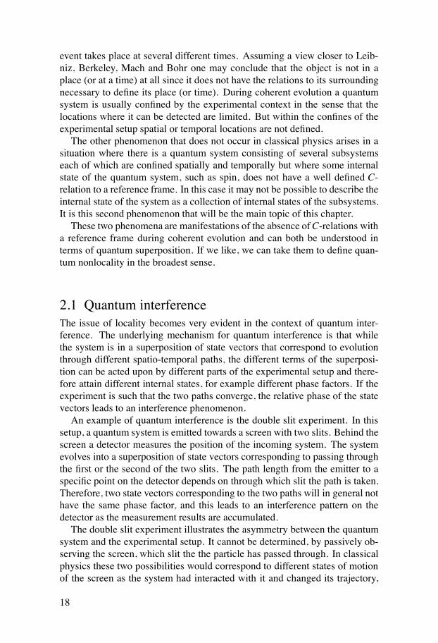
2.1 Quantum interferenceThe issue of locality becomes very evident in the context of quantum inter-ference. The underlying mechanism for quantum interference is that whilethe system is in a superposition of state vectors that correspond to evolutionthrough different spatio-temporal paths, the different terms of the superposi-tion can be acted upon by different parts of the experimental setup and there-fore attain different internal states, for example different phase factors. If theexperiment is such that the two paths converge, the relative phase of the statevectors leads to an interference phenomenon.An example of quantum interference is the double slit experiment. In this

setup, a quantum system is emitted towards a screen with two slits. Behind thescreen a detector measures the position of the incoming system. The systemevolves into a superposition of state vectors corresponding to passing throughthe first or the second of the two slits. The path length from the emitter to aspecific point on the detector depends on through which slit the path is taken.Therefore, two state vectors corresponding to the two paths will in general nothave the same phase factor, and this leads to an interference pattern on thedetector as the measurement results are accumulated.The double slit experiment illustrates the asymmetry between the quantum

system and the experimental setup. It cannot be determined, by passively ob-serving the screen, which slit the the particle has passed through. In classicalphysics these two possibilities would correspond to different states of motionof the screen as the system had interacted with it and changed its trajectory,

18

and this difference could in principle be measured to see which way the systemwent. The first interference experiment with single photons was performed in1909 [29], and the first with single electrons in 1961 [30]. Interference effectshave been demonstrated with systems as large as the C60 fullerene molecule[31].

2.2 EntanglementIn a classical system containing several spatially separated parts with internaldegrees of freedom, the internal state of the system is such that it can be de-scribed as a collection of pure internal states of the individual parts. When thisis true for a quantum system the internal state of the system is called a productstate and is described as a tensor product of states of the internal Hilbert spacesof the parts. This means that the state of the system is local in the sense that allmeasurements on a subsystem will give results that are independent of whatmeasurements has been made on the other subsystems. A mixed state that is astatistical mixture of product states is called separable.However, it is also possible for the internal degrees of freedom of the quan-

tum system to be in a state that is represented by a superposition of productstate vectors. This means that the results of a measurement on a subsystemwill in general depend on measurements made on the other parts. This phe-nomenon is called entanglement of the parts.Quantum entanglement was first discussed by Einstein, Podolsky and Rosen

[32] in 1935. They pointed out that if one assumes that physics is local, quan-tum mechanics does not give a complete description of physical phenomena.They considered two spatially separated subsystems described by a joint quan-tum state. Measurements are then performed on the two subsystems such thatthe measurements are not causally connected according to special relativity,that is, no light signals can pass from one measurement event to the other. Ifone assumes that physics is local, in the sense that one measurement cannotaffect the outcome of the other measurement, it follows that there must existinformation, in addition to that which is encoded in the quantum state vector,that determines the measurement outcomes on the two subsystems. In otherwords, there has to be local hidden variables. Since Einstein, Podolsky andRosen assumed that physics is local they concluded that quantum mechanicsdoes not give a complete description of physical reality. Einstein termed theidea that measurements, not causally connected according to special relativity,could influence each other "spooky action at a distance". The term entan-glement was coined for this nonlocal behavior in quantum mechanics shortlythereafter by Schrödinger [33].In 1964, it was shown by Bell that the measurement statistics predicted by

quantum mechanics for an entangled state was incompatible with the princi-ple of locality [34]. In other words the properties of an entangled state cannot

19

be ascribed to the parts of the system by local hidden variables. Specificallyhe showed that the correlations between measurement outcomes on two sub-systems must satisfy an inequality, the Bell inequality, if physics is local, thatis, if measurement outcomes are determined by local hidden variables. WhenBell’s inequality, and other such inequalities [35], are violated we may saythat the correlations of the system are non-local. These non-local correlationscan however not be used to transmit information superluminally [36]. Thisfeature of quantum mechanics is called signal-locality and in this sense quan-tum mechanics does not contradict the assumption that it is impossible to sendsignals faster than light, which underlies special relativity. Pure non-productquantum states violate the Bell inequality [37]. A mixed non-separable statemay however still satisfy the Bell inequality [38].Subsequently, correlations violating Bell’s inequality has been demonstrated

in experiments. In particular, a 1982 experiment by Aspect et al. was such thatthe two choices of local variables to measure were made after the emission ofthe photons [39]. Entanglement between two subsystems has also been uti-lized to teleport quantum states [40, 41].For a product state all information about the state can be obtained by per-

forming measurements on the individual subsystems. When the state is entan-gled some information can only be found by considering correlations betweenmeasurement results obtained in local measurements on different subsystems.In this case each subsystem is described as a mixed state, called the reduceddensity operator. The reduced density operator express that measurement out-comes on the subsystem are conditional on what the measurement outcomesare on other subsystems.A maximally entangled state is one for which no information about the

state can be obtained by measuring on only one subsystem. An example ofa maximally entangled state is the so called two-qubit singlet state |ψ〉 =1√2(|10〉− |01〉). For this state the reduced density operators of the qubits

are proportional to the identity operator.

2.3 Characterizing entanglementThe initial study of entanglement focused on bi-partite states. Following Bell,the entanglement of these states is described in terms of correlations betweenthe results of local measurements [35, 42]. In 1990 Greenberger, Horne andZeilinger initiated the study of entanglement in systems with more than twoparts [43]. They considered the three qubit state |000〉+ |111〉 later termed theGHZ-state. The correlations of the GHZ-state are qualitatively different fromthose of the Bell states.The difference between bi- and three-partite correlations opened up the

question of how to characterize and distinguish different kinds of entangle-ment in systems with more than two parts, that is multi-partite entanglement.

20

Characterizing entanglement is equivalent to characterizing the nonlocal prop-erties of the internal state of a quantum system. States that are equivalent un-der local unitary transformations, that is states that can be transformed intoeach other by local unitary transformations, can therefore be considered to beentangled in the same way [44, 45].Each state therefore belongs to an equivalence class of states related by

local unitary transformations, or in other words, an orbit of the group of localunitary transformations. Formally, in terms of a basis of product states, thismeans that two states in different orbits correspond to different superpositionsof state vectors which cannot be transformed into each other by local unitaryoperations. The Hilbert space of a quantum system can be decomposed intosuch orbits. A way to characterize entanglement is thus to characterize thelocal unitary orbits.In a system of n subsystems, each with a Hilbert space of complex dimen-

sion d, the real dimension of the space of normalized state vectors is 2dn−1.The maximal dimension of a group orbit assuming there are no symmetries ofthe state that reduces the dimension is n(2d− 1)+ 1. Therefore, the space oforbits is described by at least 2dn−n(2d−1)−2 parameters. As the numberof subsystems n increases the real dimension of the state space grows expo-nentially in n while the maximal dimension of a group orbit grows linearly.This means that the number of parameters of the Hilbert space that describeentanglement grows exponentially with n and it becomes a computationallyhard problem to characterize multi-partite entanglement.Let us consider a system of qubits. It has been shown that the space of orbits

for two qubits is one dimensional. For three qubits the space is parametrizedby five real parameters [44, 46]. The state space of the system can be stratifiedin terms of these parameters. For example stratifications of the two and threequbit state spaces using the second and third Hopf fibration were investigatedby Mosseri and Dandoloff [47] and by Bernevig and Chen [48].Given the increasingly rich structure of entanglement properties when the

number of subsystems grow there are many different ways to characterizethese. The characterizations can be made in terms of quantifiable entangle-ment properties but to have a complete description of the non-local propertiesit is necessary to consider non-quantifiable properties as well.A way to characterize entanglement is to consider the qualitative proper-

ties of the local unitary orbit of an entangled state. Some of these qualitativeproperties can be described in terms of the stabilizer group of the state. Thestabilizer group is the subgroup of the local unitary operations that leave thestate invariant. Examples of such qualitative properties are the dimension andtopology of the orbit. The dimension of a local unitary orbit is the dimensionof the local unitary group minus the dimension of the stabilizer group.To illustrate this we can consider a two-qubit system. An unentangled state

has a one dimensional stabilizer group of local unitary transformations. Anentangled, but not maximally entangled state has a stabilizer of dimension

21

two. A maximally entangled state has a stabilizer group of dimension three.Thus, the dimension of the stabilizer group signifies important entanglementproperties [49]. Another interesting signifier of two-qubit entanglement is thetopology of the local unitary orbit. A product state has a local SU(2)-orbit withtrivial topology, in other words it is simply connected. An entangled state onthe other hand has a doubly connected orbit [50, 51].Another way to qualitatively distinguish between unitary orbits is to con-

struct polynomials of the expansion coefficients of the state, in a basis of prod-uct states, that are invariant under local unitary transformations. These polyno-mials are called entanglement invariants. If two states are inequivalent underlocal unitary transformations there is always some entanglement invariant thattakes different values for the two states [52].The most general approach to such a qualitative characterization is to con-

sider the local SU-invariant polynomials in the expansion coefficients and thecomplex conjugates of these coefficients [53]. Such a polynomial has a ho-mogeneous degree a in the coefficients and a homogeneous degree b in thecomplex conjugates of the coefficients. These two degrees (a,b) is called thebidegree of the polynomial. If a = b the polynomial is invariant not only un-der local SU operations but under the full local unitary group. This kind ofinvariants has been studied for two, three and four qubits [54, 55, 56, 57].The polynomials for which the bidegree is (0,b) or (a,0) are invariant also

under the group of local special linear transformations SL. These are the mostgeneral invertible local operations with unit determinant that can be performedon the system. The SL operations are invertible in the sense that a state can betransformed into another state with nonzero probability of success, and trans-formed back to the original state again with nonzero probability of success.Just as for unitary operations, we can construct local SL invariant polyno-mials, and if two states are inequivalent under local SL, there will be somepolynomial invariant that distinguishes them.The widest group of local invertible operations consists of stochastic local

operations and classical communication SLOCC. These include U(1) transfor-mations in addition to local SL operations. Since the difference between localSL and SLOCC is only U(1) phase transformations the SLOCC-invariants aresimply the absolute values of the local SL invariants.Again, one can say that two states are entangled in SLOCC-inequivalent

ways if there is no SLOCC operation that transforms one state into the other.SLOCC-inequivalence is a coarser classification of entanglement than uni-tary inequivalence. Two states that are entangled in SLOCC-equivalent waysmay still be entangled in unitarily inequivalent ways. In this sense SLOCC-equivalence is the coarsest classification of entanglement types, while unitaryequivalence is the finest. For example in a three qubit system, some stateswhich cannot be distinguished by any SLOCC-invariant can still be distin-guished by a local unitary invariant, the Kempe invariant [54].

22

The algebra of entanglement invariants, whether local SU or local SL, isfinitely generated. This means that there is a finite set of polynomials fromwhich all other polynomials can be generated by multiplication and addition[58]. Therefore, studying such a generating set of polynomials is sufficient forthe characterization of entanglement by polynomial invariants.

2.3.1 SLOCC-classes and measures of entanglementWhile SLOCC-invariants do not capture the full breadth of ways in whichstates can be entangled, they correspond to quantifiable entanglement proper-ties. A SLOCC-invariant polynomial is invariant only if we do not normalizethe state after a SLOCC operation. If we do normalize, the polynomial is in-stead a function that does not increase its value under a SLOCC operation.Furthermore, this function takes its maximal value on a maximally entangledstate. Therefore, these functions are considered to be measures of entangle-ment.The states for which there exist a nonzero local SL-invariant polynomial are

called local SL-semistable [59, 60, 61]. This means that there is no finite or in-finite sequence of local SL operations, or equivalently SLOCC operations, thatcan transform the state into a state with norm zero. The states for which no lo-cal SL-invariant, and hence no SLOCC-invariant polynomial, is nonzero thereis such a sequence of SLOCC operations and these states are called SLOCC-unstable. For a local SLOCC-semistable state |ψ〉 there is always a sequenceof SLOCC operations that transform the state into a maximally entangled state[60, 62]. This sequence may be either finite of infinite. If the sequence is fi-nite the maximally entangled state is in the same SLOCC-class as |ψ〉. Ifthe sequence is infinite the maximally entangled state is in the closure of theSLOCC-class but not in the class itself.For two-qubit states there is only one class of entangled SLOCC-equivalent

states. This class is associated with a nonzero SLOCC-invariant, the concur-rence [63]. The corresponding local SL invariant of which concurrence isthe absolute value, is called the complex concurrence [50] or preconcurrence[63]. For three qubits, it was show by Dür, Vidal and Cirac that entangledstates where no qubit is in a product state with the rest of the qubits belongto one of two possible SLOCC-classes [64]. These are called theW -class andthe GHZ-class. The GHZ-class is local SLOCC-semistable and has a nonzeropolynomial invariant, the three-tangle [65]. TheW -class on the other hand isSLOCC-unstable. Furthermore, the GHZ-class contains a maximally entan-gled state, while theW -class does not.In the case of four qubits there is an infinite number of different SLOCC-

classes. These were described and categorized by Verstraeate, Dehaene, deMoor and Verschelde [66] into nine families. One of these families containSLOCC-classes that are local SL-semistable and contain maximally entan-

23

gled states, five of the families contain SLOCC-classes that are semistable butdo not contain a maximally entangled state. The last three families containthe unstable SLOCC-classes. The set of generating SL-invariant polynomialscontains four elements, one polynomial of degree two, two of degree four andone of degree six [67].For five or more qubits the SLOCC-classes have not been completely de-

scribed, and the algebra of generating polynomials is not completely known.The set of generating polynomials must contain at least 17 generators for fivequbits. It was conjectured by Luque and Thibon that the number of generatorsare precisely 17 and that they must be chosen as five polynomials of degreefour, one of degree six, five of degree eight, one of degree ten and five of de-gree twelve [68]. Later it was shown by Ðokovic and Osterloh that the set ofgenerators does contain these elements but it remains unclear if there are moreelements than this [69].

24

3. Quantum holonomies

Sometimes the properties of a system, encoded in the Hilbert space, can be di-vided into two different sets of properties that are functionally independent.By this is meant that any property from one set can be changed while allproperties from the other set remains unchanged. An example of this is thephase degree of freedom that is functionally independent of all other proper-ties. When such a decoupling is present, the Hilbert space can be describedlocally as a tensor product of two different spaces corresponding to the twosets of properties. This property of the Hilbert space is captured in the idea offiber bundles. In addition to the Hilbert space other spaces can be constructedthat have the fiber bundle structure and that are relevant in quantum mechan-ics. We will consider some examples of fiber bundles in quantum mechanicsand the related geometric structures.

3.1 Fiber bundles and parallel transportFirst we introduce some useful concepts in the context of fiber bundles. Afiber bundle E consists of a fiber manifold G and a base manifold B. The basemanifold B of the fiber bundle E is the quotient space B = E/G. Locally thefiber bundle has the structure of a tensor product between B and G. A fiberis defined by a projection π that maps the elements of E to the base. Twoelements that are mapped to the same element of B are on the same fiber. Asection of a fiber bundle is a map s : B→ E such that if x ∈ B then π(s(x)) = x,that is the composition π ◦ s acts as the identity on the base. A section is thusisomorphic to the base.A connection form A is a map from the tangent space of the base to the

tangent space of the fiber. As such, it relates an infinitesimal motion in thebase to an infinitesimal motion on the fiber. This rule for how to move on thefiber when moving on the base defines a notion of parallel transport.A connection form transforms under a change of basis in the fiber given by

a transformation g as

A→ g−1dg+g−1Ag. (3.1)

Connection forms in physics are also called gauge potentials. An example ofa gauge potential is the magnetic vector potential in electromagnetism. To theconnection form one can associate a curvature tensor Ω defined as

25

Ω = dA+A∧A, (3.2)

which transforms as g−1Ωg. Since the curvature tensor can be interpretedas a describing a geometry, a choice of connection is a way to give the basespace a geometry. The curvature tensor of the magnetic vector potential is theelectromagnetic field strength.The accumulated movement along the fiber that is given by the connection

for a given closed path in the base is called the holonomy of the path. Anexample of a holonomy is a vector located at the north pole of a sphere thatoriginally points towards the south pole along the surface of the sphere, andthen is transported along a closed curve while still pointing towards the southpole. The transported vector will in general be rotated relative the originalvector and this is due to the curvature of the surface of the sphere.

3.2 Abelian geometric phasesThe U(1) degree of freedom becomes important in setups that allow quantuminterference. The related U(1)-bundle structure of Hilbert space of a quantumsystem can be used to give the state space a geometry through a constructioncalled the geometric phase [70]. The geometric phase is a U(1) holonomy ofa cyclic evolution. The origin of the geometric phase can be traced to a par-allel transport condition developed in the context of classical optics by Pan-charatnam in 1956 [71]. The same parallelity condition was rediscovered ina quantum mechanical context by Berry in 1984 [72]. This condition can beillustrated with a Mach-Zehnder interferometer.In the Mach-Zehnder interferometer, a photon is emitted by a source to-

wards a beamsplitter (half-silvered mirror). This creates two optical pathssince there is an optical path corresponding to transmission through the beam-splitter and one optical path corresponding to reflection. The two paths arethen rejoined at a second beamsplitter. The setup is such that the photon can-not be detected anywhere in between the beamsplitters. Therefore, it is notoperationally constrained which path it takes and the state of the photon there-fore evolves into a superposition of state vectors corresponding to the twodifferent paths. This superposition leads to an interference effect that is de-pendent on unitary transformations performed locally in the paths. If someunitary operationU is introduced in one of the optical paths and a U(1) phaseshift χ is introduced in the other the interference intensity is

I =12

+12Re(〈ψ |e−iχU |ψ〉), (3.3)

where |ψ〉 is the initial internal state of the photon. The Mach-Zehnder inter-ferometer is illustrated in figure 3.1.

26

Figure 3.1. The Mach-Zehnder interferometer. A general unitary operationU is performed inone of the arms of the interferometer and a phase shift χ is introduced in the other arm.

The essential idea of the Pancharatnam parallelity condition is that the lightbeams corresponding to the two paths of the Mach-Zehnder setup prior to thelast beamsplitter are defined to be in-phase, or parallel, if their relative phase χis adjusted such that the Mach-Zehnder intensity is maximized. In the contextof quantum mechanics, the analogue parallelity condition is a condition forstate vectors in Hilbert space. Two state vectors, corresponding to the twopaths of the Mach-Zehnder interferometer, are parallel if their relative phaseχ is adjusted to maximize the interference intensity.Using this idea of parallelity one can construct a parallel transport condi-

tion. A state is said to be parallel transported along a path in its Hilbert space iffor every point on the path the instantaneous state vector is parallel to the statevector of the evolution immediately preceding it in the infinitesimal sense.Geometrically this means that the infinitesimal change d|ψ(t)〉 of the statevector |ψ(t)〉 must be orthogonal to |ψ(t)〉. This parallel transport conditionis captured as

〈ψ(t)| ddt|ψ(t)〉 = 0, (3.4)

where we have assumed that |ψ(t)〉 is a normalized state. This is the infinites-imal version of the Pancharatnam parallelity condition. Thinking again ofthe Hilbert space as a U(1) bundle, we may express the state on a form thatmakes the bundle structure explicit. We introduce a state |ϕ(t)〉 defined by|ψ(t)〉 ≡ eiγ(t)|ϕ(t)〉 where γ(0) = 0 and |ϕ(T)〉= |ϕ(0)〉. This |ϕ(t)〉 definesa section that is isomorphic to the projection of |ψ(t)〉 onto the projectiveHilbert space. We can see that using this section the parallel transport condi-tion in equation (3.4) implies that

27

idγ(t)dt

+ 〈ϕ(t)| ddt|ϕ(t)〉 = 0. (3.5)

This equation describes how the parallel transport condition determines a mo-tion in the fiber given a motion in the section. But since the section is locallyisomorphic to the projective Hilbert space we can pull back the connection tothe projective Hilbert space. In this sense, we can essentially identify a mo-tion in the section with a motion in the projective Hilbert space. The objecti〈ϕ(t)| ddt |ϕ(t)〉 is the connection form associated with the parallel transportcondition. As such, the connection form gives the projective Hilbert space ageometry. A change of coordinates on the fiber such that |ϕ(t)〉→ ei f (t)|ϕ(t)〉induces a transformation of the connection as

〈ϕ(t)| ddt|ϕ(t)〉 → e−i f (t)

ddtei f (t) + e−i f (t)〈ϕ(t)| d

dt|ϕ(t)〉ei f (t). (3.6)

Thus, the connection transforms as a proper gauge potential.Integrating equation (3.5) for a closed curve in projective Hilbert space

gives us an accumulated phase

γ(T) = i∫ T

0〈ϕ(t)| d

dt|ϕ(t)〉dt. (3.7)

This global phase factor eiγ(T) is a function of the path in projective Hilbertspace only and is invariant under reparameterizations of the fiber. It is in otherwords independent of the choice of section. The global phase γ(T) is thereforecalled the geometric phase of the evolution [70].In general, the global phase φ acquired by the state in a cyclic evolution

will be different from the geometric phase. The global phase can be dividedinto a geometric phase γ and a dynamical phase δ that is determined by theHamiltonian of the system. The global phase is given by the expression

φ = −∫ T

0〈ψ(t)|H(t)|ψ(t)〉dt+ i

∫ T

0〈ϕ(t)| d

dt|ϕ(t)〉dt, (3.8)

where the first term on the right-hand side is the dynamical phase. One simpleway to realize parallel transport is to evolve a quantum system adiabaticallysuch that it remains in the zero energy ground state of a Hamiltonian through-out the evolution. This is the setting in which Berry originally constructed thequantum geometric phase [72]. The construction of geometric phases has alsobeen extended to mixed states [73] and to dissipative evolution [74].

28

3.3 Non-Abelian geometric phasesThe concept of U(1) geometric phases for cyclic evolution of states can be gen-eralized to non-Abelian geometric phases for cyclic evolution of subspacesof Hilbert space [75, 76]. Consider an L-dimensional subspace M(t) of anN-dimensional Hilbert space. Suppose that this subspace undergoes a cyclicevolution so that M(0) = M(T ). In M(t) we can introduce a time dependentorthonormal basis of state vectors |ψ j(t)〉 where j= 1, . . . ,L. These state vec-tors are evolving according to the same Hamiltonian as M(t). In addition tothis we can introduce another orthonormal basis |ϕ j(t)〉, j= 1, . . . ,L, such that|ϕ j(0)〉 = |ϕ j(T )〉 for all j. Then the relation between the two orthonormalbases can be expressed by a unitary matrixU as

|ψ j(t)〉 =L

∑k=1

Uk j(t)|ϕk(t)〉. (3.9)

Consider now the time evolution of |ψ j(t)〉 given by the Schrödinger equa-tion i ddt |ψ j(t)〉 = H(t)|ψ j(t)〉 and substitute |ψ j(t)〉 for |ϕ j(t)〉 according toequation (3.9). Multiply the right- and left-hand sides of this equation with|ϕl(t)〉, yielding

iddtUl j(t)+ i

L

∑k=1

Uk j〈ϕl(t)| ddt |ϕk(t)〉 =L

∑k=1

Uk j〈ϕl(t)|H(t)|ϕk(t)〉. (3.10)

If we define Alk = i〈ϕl(t)| ddt |ϕk(t)〉 and Klk = 〈ϕl(t)|H(t)|ϕk(t)〉, equation(3.10) can expressed as a matrix equation

iddtU(t)+A(t)U(t) = K(t)U(t)⇒ i

(ddtU(t)

)U†(t) = K(t)−A(t). (3.11)

The matrix A is independent of the Hamiltonian. The time integral of equation(3.11) is

U(t) = Pe∫ t0 i(A(τ)−K(τ))dτ , (3.12)

where P denotes path ordering. If we reparametrize the subspace through aunitary transformation G we see that A transforms as

A→ iG†ddtG+G†AG. (3.13)

So A generalizes the connection form i〈ϕ(t)| ddt |ϕ(t)〉 of the Abelian geometricphase and transforms as a proper gauge potential.

29

The parallel transport condition of a state |ψ(t)〉 corresponding to this con-nection is

〈ϕl(t)| ddt |ψ(t)〉= 0, l = 1, . . . ,L. (3.14)

Thus, a state is parallel transported if the infinitesimal change in each in-finitesimal time step is orthogonal to every basis vector |ϕk(t)〉 of the subspaceM(t). This corresponds to K(t) = 0 for all t, and therefore we may considerPe

∫ t0 iA(τ)dτ to be the non-Abelian generalization of the geometric phase. Since

K(t) generalizes the term responsible for the dynamical phase in the Abeliancase, we can say that the condition for zero dynamical contribution is thatKlk = 〈ϕl(t)|H(t)|ϕk(t)〉 = 0 for all |ϕk(t)〉. An example of evolution withzero dynamical contribution is adiabatic evolution of the subspace, where thesubspace remains in the zero energy subspace of the slowly varying Hamilto-nian during the entire evolution, in the adiabatic limit. This situation is wherenon-Abelian holonomies were first considered [75].After a cyclic evolution during the time interval [0,T ] the subspace returns

to its original position but the orthonormal basis has been transformed by theunitary U(T). The space of all L-dimensional subspaces is called the Grass-mann manifold G(N;L). Thus, the subspace has followed a closed path inG(N;L). The set of all orthonormal bases of the L dimensional subspacesforms a manifold called the Stiefel manifold S (N;L). The Stiefel manifoldcan be viewed as a fiber bundle with G(N;L) as a base and the set of L×L di-mensional unitary matrices as the fiber space. The holonomyU(C) associatedto a pathC in G(N;L), as given by

U(C) = Pe∫C(τ) iA(τ)dτ , (3.15)

where P denotes path ordering, can therefore be considered as a holonomy ofa Stiefel manifold [76].

3.4 Lévay holonomyThe Hilbert space of normalized state vectors of a qubit is isomorphic to thethree-sphere S3. This can be seen by noting that a non-normalized qubit statevector is isomorphic to a vector in C

2, or equivalently a vector in R4. Theset of normalized vectors with norm 1 in R

4 is precisely S3. The U(1) bundlestructure for this Hilbert space is described by the first Hopf fibration S1 ↪→S3 ↪→ S2, where the fiber U(1) is isomorphic to the one-sphere S1, and the baseis isomorphic to the two-sphere S2.The Hilbert space of normalized state vectors for two qubits is isomorphic

to S7. S7 can be fibrated in the second Hopf fibration as S3 ↪→ S7 ↪→ S4. While

30

the fiber of the first Hopf fibration is isomorphic to the unit complex numbers,the fiber S3 of the second Hopf fibration is isomorphic to the unit quaternions.This analogy led Mosseri and Dandoloff [47] to introduce a description of

two-qubit states as unit quaternionic vectors. A two qubit state with ordinarycomplex vector representation

|ψ〉 = α |00〉+β |01〉+ γ |10〉+δ |11〉, (3.16)

where α ,β ,γ ,δ ∈ C, is in this representation instead represented as a quater-nionic state vector

|Ψ〉 = (α +β j) |0〉+(γ+δ j)|1〉. (3.17)

Here i, j and k are the standard quaternionic basis elements and satisfy i2 =j2 =k2 =−1 and ij=−ji= k. The basis vector |0〉 correspond to the subspacespanned by |00〉 and |01〉, and the basis vector |1〉 to the subspace spannedby |10〉 and |11〉. The group of unit quaternions is isomorphic to SU(2) androtations in the subspaces defining |0〉 and |1〉 are given by quaternion phasefactors. Therefore, in this representation an SU(2) operation on the secondqubit corresponds to multiplication by a unit quaternion from the right. AnSU(2) operation on the first qubit on the other hand corresponds to an SU(2)operation from the left.To complete the analogy between the one-qubit complex vector representa-

tion and the two-qubit quaternionic representation, Lévay [77] introduced thequaternionic analogue of the Pancharatnam connection:

〈Ψ(t)| ddt|Ψ(t)〉 = 0. (3.18)

To make an explicit construction of the quaternionic analogue to the geometricphase one can introduce a section on the bundle. By defining |Φ(t)〉 through|Ψ〉 = |Φ〉q(t), such that |Φ(0)〉= |Φ(T )〉 and q(0) = 1, the parallel transportcondition can be expressed as

q(t)〈Φ(t)| ddt|Φ(t)〉q(t)+ q(t)

ddtq(t) = 0. (3.19)

The first term q(t)〈Φ| ddt |Φ〉q(t)≡ A can be identified as the quaternion-valuedconnection form, where q is the quaternionic conjugate of q. In a cyclic evolu-tion satisfying the parallel transport condition, the accumulated quaternionicgeometric phase is

q(T ) = Pe∫ T0 A(t)dt , (3.20)

where P denotes path ordering.

31

3.5 Aharonov-Bohm phaseIn 1959 Aharonov and Bohm [78] described an interference effect related tothe magnetic vector potential. In classical electrodynamics the vector potentialdoes not have a physical meaning. All physical effects can be derived from theelectric and magnetic fields and in the absence of such fields a charged particleis not affected by any forces.In quantum mechanics a charged particle moving in a magnetic vector po-

tential A(R), where R is the spatial coordinate, acquires a phase shift. In-finitesimally the phase shift is proportional to A(R) · dR. To construct anexperiment where this phase shift has physically measurable consequences,Aharonov and Bohm conceived of a setup involving electrons where the pathof the electrons is split into two paths c1 and c2 that reconverge at a later point.Enclosed by the two paths is located a solenoid and a magnetic field that isconfined to the solenoid. The magnetic field is zero outside the solenoid butthe vector potential A(R) is not. This is illustrated in figure 3.2.

Figure 3.2. The Aharanov-Bohm setup. The electron path bifurcates into two paths c1 and c2that together enclose a solenoid.

The two paths c1 and c2 correspond to different phase changes due to thevector potentialA. The electron injected into the setup will evolve into a super-position of state vectors corresponding to the two paths and these two vectorswill accumulate different phase factors. This leads to an interference phe-nomenon that can be observed. The phase difference between the two pathsis the integral

∫cA(R) ·dR of the magnetic vector potential A(R) along the

closed path c = c1− c2. This is a phenomenon that is impossible in classicalelectrodynamics since a classical electron must follow either the path c1 or c2.If the paths c1 and c2 are continuously deformed without entering the solenoid

the Aharonov-Bohm phase remains the same. If the paths are chosen such thatthey could be continuously deformed to a point without crossing the solenoid,that is, if c is contractible, the relative phase would vanish. These proper-ties follows immediately from Stokes’ theorem and illustrate that the phasedepends only on which homotopy class of curves, that do not intersect thesolenoid, c belongs to. In this sense the Aharonov-Bohm phase is a topologi-cal phase.

32

4. Quantum computation

The idea of using quantum systems to perform computations was first dis-cussed in the early 1980s by Benioff [79, 80], Feynman [81] and Deutsch[82]. In this chapter we briefly review some of the ideas, motivations behind,and challenges for realization of quantum computation. The basic idea ofquantum computation is to exploit coherent evolution and entanglement of aquantum system to perform computational tasks. Since quantum systems be-have differently from classical systems this allows for algorithms that cannotbe implemented on a classical computer.

4.1 Quantum circuitThe standard model of classical computation is the Boolean circuit model. Inthis model a computer is a collection of wires and logical gates. The inputis represented as a collection of Boolean variables taking the values 0 or 1,called bits. The input bits are inserted into and carried around by the wires andare operated upon by logical gates that are implementing a Boolean functionon the bits, as illustrated in figure 4.1. Each circuit that can be constructedcorresponds to a question about the input and the output of the circuit is theanswer to this question.

Figure 4.1. The circuit model of computing.

The most common proposal for quantum computation is the quantum cir-cuit model. Quantum circuits are direct analogues of the Boolean circuits inthe sense that bits are replaced by qubits and classical logic gates are replacedby quantum gates. The input is constructed by preparing the state of a col-lection of qubits in the register of the computer. After a sequence of gate

33

operations has been performed on the qubits in the register a measurement isperformed and the result of this is the output of the computation. Quantumgates are typically chosen as unitary operations acting on the qubits. Quantumcircuits can in fact be constructed solely out of unitary gates. Such a circuitleads to an operation on the input that is reversible, unlike most classical cir-cuits.Alternative proposals to the quantum circuit model include measurement

based quantum computation [83] and adiabatic quantum computation [84].

4.2 UniversalityA universal computer is a machine that can perform any physically possiblecomputation. Universal computers are possible both in the classical and quan-tum theory of computation. In 1985, Deutsch described the first quantum al-gorithm and showed that universal quantum computation is possible [82]. In acircuit based quantum computer, universal quantum computation requires thatan arbitrary quantum gate operation can be performed. A universal set of gatesis a set of gates such that an arbitrary quantum gate can be built using gatesfrom this set. A set of universal quantum gates can be chosen as the set of allone qubit gates in conjunction with the two-qubit exclusive-OR gate as shownby Barenco et al. [85]. The exclusive-OR gate maps the Boolean values x,y tox,x+y where addition is with modulus 2. This result shows that any operationon a set of qubits can be performed using only one- and two-qubit gates. Laterit was shown that the two-qubit gate that needs to be chosen to make the setuniversal can be chosen as any entangling two-qubit gate [86]. A two-qubitgate is entangling if it creates entanglement between two qubits initially ina product state. Moreover, any two non-commuting one-qubit gates are suf-ficient to perform an arbitrary single qubit operation [87]. It has also beenshown that almost any two-qubit gate on its own is a universal set [87, 88]. By"almost any gate" is meant that if a gate is selected randomly from the set ofall gates the probability to select a non-universal gate is zero.

4.3 Computational complexityA computational problem is called computable if there exists a classical al-gorithm that solves it. The computational complexity of a problem is givenby the amount of time (or other resources) the best known classical algorithmrequires to solve the problem. One way to classify this computational com-plexity is to measure how the number of gates necessary to solve a problemincreases with the size of the input. Problems for which the required numberof gates, when using a deterministic algorithm, scales as a polynomial in theinput size are called P. Problems that can be solved by a non-deterministic al-

34

gorithm, that is an algorithm that can prescribe multiple parallel actions for agiven input, with a polynomial scaling are called NP. The set of P problemsis a subset of the NP problems. However, it is not currently known if all NPproblems could in fact be reduced to P problems since the most efficient al-gorithm to solve a problem may not have been found. This question of therelation between P and NP problems was first stated by Cook [89] and is con-sidered to be a major problem in computer science. However, it is suspectedthat NP problems are not generally reducible to P problems.A problem generally thought to be NP for classical algorithm is prime fac-

torization of integers. In 1994 it was shown by Shor that there is a quantumalgorithm that solves the prime factorization problem and scales polynomially[90]. Prime factorization belongs to a class of problems that can be solved by aquantum algorithm with a probability of error at most 1/3 and with a polyno-mial scaling behavior. This class is called BQP and it has been speculated thatthere could be a large set of problems classified as NP problems that belong tothis class.An example where it has been proven that a quantum algorithm is more

efficient than any classical algorithm is Grovers search algorithm [91]. Whensearching an unsorted data set it has been proven that there is no classicalalgorithm for which the number of gates that is required increases slower thanlinearly as a function of the size of the database. Grovers algorithm insteadrequires a number of gates that scales proportionally to the square root ofthe size. While the search is a P problem, this still represents a considerableimprovement. While the most efficient classical algorithms may not have beenfound it is thus at least clear that some quantum algorithms can solve somecomputational problems faster than any classical algorithms.With regards to alternatives to quantum circuits, it has been shown that any

algorithm in a quantum circuit can be simulated using a measurement basedcomputer or an adiabatic computer, and that the difference in time requirementis polynomial [83, 92].

4.4 Fault toleranceThe experimental realization of quantum circuits and quantum algorithms hasproven to be very challenging. One reason for this is that quantum comput-ing relies on coherent evolution of a quantum system. Decoherence due toopen system effects can however never be completely eliminated in a phys-ical system. Different physical systems where quantum computers could beimplemented have different decoherence times. Another source of error isinstabilities of the setup leading to the incorrect gate operations being per-formed. The decoherence time of the system and the instability of the setuplimit the number of gates that can be implemented before the probability of anerroneous result becomes too large. To be able to construct a quantum com-

35

puter that is reliable enough to be of practical use it is thus necessary to find animplementation of the computer in a physical system that is not too suscepti-ble to instabilities of the setup and has a long decoherence time relative to thetime required to implement a gate.A commonmeasure of the robustness of a gate is the probability of error per

gate operation. Depending on the complexity of the computational task thatone wants to implement and the nature of the sources of error different levelsrobustness must be achieved. The threshold level of error per gate that must bereached to make quantum computation practically useful has been estimatedin different settings to be between 10−6 [93, 94] and 10−4 [95] and even ashigh as 10−3 [96] or 10−2 [97].If the error rate can be made sufficiently low it is thought to be possible to

use error correction protocols to make the computation reliable. Classical errorcorrection protocols often rely on the creation of copies of the information butsince cloning of quantum states is impossible these protocols cannot be used.It was therefore unclear if quantum error correction was possible until the firstsuch protocols were introduced by Shor [98] and Steane [99]. These protocolsuse entanglement by encoding the computational qubits in states of entangledmulti-qubit systems.Some proposals to achieve fault tolerant quantum computation use struc-

tures that are thought to be inherently more stable to errors. Examples of suchare holonomic quantum computation using non-Abelian geometric phases [100],and topological quantum computation using anyons [101]. A geometric two-qubit gate has been implemented using geometric phases with an error rate of3×10−2 in trapped ions [102].

36

5. Correlation induced quantum holonomies:Paper I

In two-particle interferometry a system consisting of two subsystems is emit-ted from a source in such a way that the two parts are separated. Each sub-system is emitted into an interferometer and interference intensities are mea-sured. By choosing the interferometer settings properly one can have a situa-tion where each individual detector does not register any interference pattern,but when coincident detections are considered an interference pattern emerges[103, 104, 105].

5.1 Franson interferometryThe Franson interferometer [106, 107] is a kind of two-particle interferometerthat makes use of a quantum system in a temporal superposition. In the Fran-son interferometric setup, the source of the photon pair is such that no time ofemission is operationally defined.The setup is composed of two identical unbalanced two path interferome-

ters, called Franson loops. The two photons are emitted one into each Fransonloop. In each loop a beamsplitter divides the optical path into two opticalpaths of unequal length that reconverge at a second beamsplitter. Detectorsare placed after the reconvergence of the optical paths and coincidence mea-surements are made.Due to the fact that no time of emission is operationally defined, each pho-

ton can be in a superposition of a state vector that corresponds to being emittedat an earlier time and taking the long path to the detector, and a state vectorthat corresponds to being emitted at a later time and taking the short path tothe detector.The difference in path length between the two paths in each Franson loop

is chosen such that it is longer than the one-photon coherence length. In thisway no one-photon interference occurs. The difference in path length is alsochosen shorter than the two-particle coherence length. Furthermore, the timeresolution of the detectors must be smaller than the difference in travel timebetween the long and short path.If these conditions are satisfied, and if a coincidence is detected, the photon

pair was in a superposition of state vector corresponding to the two photonsboth taking the short path, and a state vector corresponding to the two photonstaking the long paths.

37

5.2 Correlation induced holonomiesIn paper I we introduce a parallel transport condition in the context of Fransoninterferometry that is analogue to that of the Pancharatnam parallel transportcondition in the Mach-Zehnder setup. We consider a Franson interferometricsetup where the emitted system is a general bi-partite system and where thetwo subsystems have internal degrees of freedom with state spaces of dimen-sion DA and DB respectively.

Figure 5.1. The Franson interferometer setup. Unitary operations on the internal degrees offreedom of the subsystems are performed in the long arms of each Franson loop.

We consider the situation where unitary operationsU and V are performedon the internal degrees of freedom of the subsystems in the long arms of Fran-son loops. The internal state of the system after the second beam-splitters,corresponding to the coincidence detections, is then given by

ρ =14(1+U⊗V )ρ0(1+U†⊗V †), (5.1)

where ρ0 is the initial internal state of the system and the resulting coincidenceintensity IAB is

IAB =12

+12ReTr(U⊗Vρ0). (5.2)

In the Pancharatnam construction the relative phase of the two paths of theMach-Zehnder interferometer was adjusted by a phase shift operation suchthat the interference intensity is maximized. In [108] this construction wasgeneralized to the Franson interferometer by introducing a phase shift in theshort arms of one of the Franson loops of the setup in figure 5.1. In paper Ia different generalization of the Pancharatnam construction is introduced. Aunitary operationU is chosen in one of the Franson loops, and, given this uni-tary, the question is what operation V must be chosen in the other Franson

38

loop in order to maximize the coincidence intensity? The operatorU evolvesthe input state ρ0 to U⊗1ρ0U†⊗1. The operation V is chosen to maximizethe coincidence intensity and plays the same role as the phase shift χ in thePancharatnam construction. The condition of maximal coincidence intensitywith respect toV defines a kind of parallelity between the state ρ0 correspond-ing to the short-short path and the state U⊗Vρ0U†⊗V † corresponding to thelong-long path. Parallelity between states in an evolution generated by U(t)and V (t) that are infinitesimally close is then defined by a connection formA(t), that takes the form

A(t) =D2B−1∑l,k=0

D2A−1∑j=0

1[δ0 j(DA−2)+2]

Tr(dU(t)U†(t)χAj )S jk(t)B−1lk (t)χBl , (5.3)

where B−1 is the inverse of a matrix given by Bjk = ReTr(1⊗χBj χBk ρ(t)) and

S jk = Tr(ρ(t)χAj ⊗χBk

). Here {χAk } and {χBk } are the generators of SU(DA)

and SU(DB) respectively. The matrix B is generally not easy to invert andtherefore the form of the connection is not given explicitly. A state is paralleltransported if dV (t)V †(t) =A(t) for all t. Parallel transport along a closed pathC(t), t ∈ [0,T ], in the sense that ρA(0) = ρA(T ) where ρA = TrB(ρ), leads tothe holonomy

V (T ) = Pe∫ T0 A(t)dt , (5.4)

where P denotes path ordering. This holonomy is non-Abelian in the generalcase. However, if the initial internal state ρ0 is a product state the holonomywill be a U(1) phase factor. Therefore, the holonomy group is Abelian forproduct states. Thus, the non-Abelian character of the holonomy group in thegeneral case stems from the correlations in the internal degrees of freedombetween the two subsystems. For this reason we say that the holonomy inequation (5.4) is correlation induced when it is non-Abelian.An important special case is a system of two qubits and a restriction on the

operatorsU and V to SU(2). The simple structure of SU(2) makes it possibleto express the parallel transport condition as

dV (t)V †(t) = −3

∑j,k=1

Tr(dU(t)U†(t)σk)Mk jσ j, (5.5)

where Mk j = Tr(ρσk⊗ σ j). In this case the parallel transport condition isidentical to the parallel transport condition introduced by Lévay [77]. To seewhy let us first express the coincidence intensity of the Franson interferometerusing the quaternionic state representation of chapter (3.4):

39

I =12

+12Re(〈Ψ|U|Ψ〉qV), (5.6)

where qV is the unit quaternion corresponding to the operator V . This is thequaternionic quantum mechanics [109] analogue of the Mach-Zehnder inter-ference intensity in equation (3.3) given that an SU(2) unitary has been appliedto one of the arms of the interferometer and a quaternionic phase shift qV hasbeen introduced to the other. This is illustrated in figure 5.2.

Figure 5.2. Correspondence between Franson setup and quaternionic quantum mechanicsMach-Zehnder setup.

In this sense, the Franson interferometer behaves like a Mach-Zehnder in-terferometer in quaternionic quantummechanics. It is important to note that inquaternionic quantummechanics the absolute quaternionic phase is not an ob-servable quantity, while in this case it corresponds to a rotation of the secondqubit and is thus measurable. The Lévay connection, which is the analogue ofthe Pancharatnam connection for quaternionic qubits, is

〈dΨ|Ψ〉= dqV∗qV + 〈dΨ|UdU†|Ψ〉. (5.7)

From these observation it becomes clear that Lévay’s parallel transport [77]is identical to the parallel transport introduced in paper I when evolution isrestricted to local SU(2) evolution of qubit pairs. Thus we have seen thatthe Franson interferometer in this representation corresponds to the quater-nionic quantum mechanics analogue of the Mach-Zehnder interferometer. Italso gives an operational interpretation of Lévay’s geometric phase.

40

6. Topological phases and multi-qubitentanglement: Paper II

The concept of global phase factors originating from the topological structureof group orbits in projective Hilbert space, called topological phases, was in-troduced by Milman and Mosseri [50]. The basic idea is that in some cases theglobal phase acquired by the state of a quantum system undergoing a cyclicevolution in its projective Hilbert space generated by local special unitary op-erations will confer information about the topology of the local special unitaryorbit of the state. This conception of topological phases is distinct from topo-logical phases of the Aharonov-Bohm kind (see section 3.2), but share theproperty that they only depend on the homotopy classes of the evolution insome space.

6.1 Definition of topological phasesA quantum system initially in pure state |ψ〉, that undergoes evolution througha continuous closed path in its projective Hilbert space by action of a Lie-groupG, acquires a global phase factor eiχ , where χ ∈ C. We allow χ to be a com-plex number to include the most general case of dissipative evolution. Thephase factor is determined by the G-action and the state. In some cases |ψ〉and G are such that only a discrete set of phase factors can result from closedpath evolution. Then two closed paths associated with different phase factorscannot be continuously deformed into each other since this would require thephase factor to change continuously through the forbidden intermediate val-ues. Two such closed paths hence belong to different homotopy classes with|ψ〉 as the base point, on the G-orbit over |ψ〉. The G-orbit over |ψ〉 is theimmersed submanifold OG

|ψ〉 = {g|ψ〉 | g ∈ G, |ψ〉 ∼ λ |ψ〉, λ ∈ C\{0}} ofprojective Hilbert space. The discreteness of the set of possible phase factorsthus implies that the topology of OG

|ψ〉 is non-trivial in the sense that it is notsimply connected.The set of phase factors eiχ associated with cyclic G-evolutions of a state

|ψ〉 are the solutions of the equations of the form

g|ψ〉 = eiχ |ψ〉, g ∈ G, χ ∈ C. (6.1)

The phase factors eiχ and the associated cyclic evolutions are closely relatedto stabilizers of the state |ψ〉 in the sense that if gχ ∈ G is a group element

41

giving the topological phase χ , i.e., gχ |ψ〉 = eiχ |ψ〉, it is also a stabilizer ofthe state in projective Hilbert space. To study topological phases one can thusstudy G-stabilizers.This definition of topological phases is not specific to any particular group,

but we will focus on topological phases that arise under local SU evolution.

6.2 Topological phases in bi-partite systemsThe first system where topological phases, as a result of local SU(2) evolu-tion, were described was that of two maximally entangled qubits [50]. Thelocal SU(2) orbit of a maximally entangled state has the topology of SO(3)[110]. SO(3) can be visualized as the unit 3-ball with opposite points on thesurface identified. Using this picture, one can see that there are two homo-topy classes of closed curves in SO(3). One homotopy class consists of thecontractible closed curves. These are contained in the interior of the ball, orintersect the surface of the ball an even number of times. The other class isthe closed incontractible curves that intersect the surface of the ball an oddnumber of times. This is illustrated in figure 6.1

Figure 6.1. SO(3) visualized as a 3-ball with antipodal points on the surface identified. Rep-resentatives of the two homotopy classes of closed curves.

Milman and Mosseri showed that if a maximally entangled two-qubit stateis evolved by local SU(2) operators along a closed curve belonging to thehomotopy class of contractible curves, it accumulates a 2π phase. If the curveis incontractible on the other hand, it accumulates a π phase. These topologicalphases for two qubits have been observed experimentally in the context ofpolarization and spatial mode transformations of a laser beam [111], and inthe context of NMR [112]. The topological phases are present also in non-maximally entangled states, but are absent in product states. In other words,

42

the existence of topological phases in the case of two qubits requires a nonzeroconcurrence. Two qubit product states can accumulate an arbitrary phase asthe result of local SU(2) evolution through a closed path in projective Hilbertspace.Topological phases have also been shown to exist in entangled two-qudit

systems by Oxman and Khoury [113]. In the case of two-qudits the topo-logical phases are present only if the determinant of the coefficient matrix isnonzero. For a two-qudit state, |ψ〉 = ∑d

i, j=1bi j|i j〉, the coefficients form ad× d matrix with elements bi j. The determinant of the coefficient matrix istherefore an SU(d)⊗ SU(d) invariant polynomial of homogenous degree d.Thus, a nonzero value implies that the two qudits are entangled. The possibletopological phases in this case are the multiples of 2πd , where again the con-tractible curves are associated with the trivial phase 2π . For two qubits thedeterminant of the coefficient matrix is a factor 12 times the complex concur-rence.

6.3 Topological phases in multi-qubit systems andentanglement

As seen in the case of two qubits the topological phases are only present whena SLOCC invariant is nonzero. This is a special case of a more general pic-ture. The existence of an SU-invariant polynomial of bidegree (a,b), wherea �= b, is a sufficient condition for the existence of topological phases in ann-qubit system. The reason for this is that when the state is multiplied by aphase factor eiφ such a polynomial will be multiplied by a phase factor ei(a−b)φand since the polynomial is invariant under local SU operations it must holdthat ei(a−b)φ = 1. This implies that φ = n2π

a−b for some n. For a particular state|ψ〉 the degrees of the generators of the algebra of nonzero local SU invariantpolynomials, put restrictions on which topological phases that can exist. Moreprecisely, if there are m nonzero generators no other phases than multiplesof 2π

gcd(d1,...,dm), where gcd(d1, . . . ,dm) is the greatest common divisor of the

degrees d1, . . . ,dm of the generators, can possibly exist. Since the generatorsalso provide a classification of the entanglement properties this establishes aconnection between the concepts of topological phases and multi-partite en-tanglement.If the state is such that one qubit is in a product state with the rest of the

qubits, there will be no topological phases. This follows directly from the factthat for a single qubit a cyclic SU(2) evolution can give the state an arbitraryphase factor. Furthermore, a state of the form |ψ〉 = |ρ〉⊗ |θ 〉 has a topolog-ical phase χ if and only if |ρ〉 and |θ 〉 have topological phases χρ and χθ ,respectively. In such a case χ = χρ +χθ .The topological phase accumulated by a system is a global phase. In other

words, it is accumulated through an evolution and is thus generally composed

43

of both a dynamical and a geometric phase, but is independent of the Hamilto-nian driving the system and continuous deformations of the path in projectiveHilbert space. It is thus clear also from this perspective that topological phasescannot in general be associated with the geometry of the projective Hilbertspace, but must be associated with the topology.If the state of the system is maximally entangled, and thus all reduced den-

sity matrices of the individual subsystems are maximally mixed, the dynamicalphase is zero for all evolutions. In this case, the topological phase is identicalto the geometric phase of the evolution. This follows from the fact that theHamiltonian generating the local SU evolution is traceless and decomposesinto a sum of local Hamiltonians for the subsystems. This means we can reex-press 〈ψ |H|ψ〉 as

〈ψ |H|ψ〉=∑iTr(Hiρi) = 0, (6.2)

where Hi is the Hamiltonian generating the SU evolution of subsystem i andρi is the reduced density operator. Thus the dynamical phase for this class ofstates is identically zero.Since each topological phase is associated with a stabilizer, or possibly a

set of stabilizers, states related by SLOCC operations that share a set of stabi-lizers will share a topological phase. Given a state |ψ〉 with stabilizer U anystate related to |ψ〉 by a SLOCC operation that diagonalize in the same basisas U will share the stabilizer U . Furthermore, a state related to |ψ〉 by a uni-tary transformation V will have the same topological phases and a conjugatedstabilizer VUV †. Therefore, one can define an equivalence class in terms of acommon stabilizer, up to conjugation, with associated topological phase. Thisis termed the A-class associated toU in paper II.The condition a n-qubit state must satisfy to have topological phases can

be expressed as an algebraic condition. We consider a representation of thestate in a basis of product states. The vectors of such a representation areexpressed formally as a string of 0s and 1s. Such a string corresponds to acoordinate vector in Z

n with coordinates given by the string. For a state tohave topological phases it must hold that for every representation of the statein terms of a product basis, that the basis vectors included in the expansion ofthe state, when viewed as vectors in Z

n, are linearly dependent.The different possible linear dependence relations between such sets of vec-

tors can be expressed in terms of combinatorics. To find the possible topologi-cal phases in an n-qubit system it is sufficient to consider the subset of such lin-ear dependence relations, namely those involving n+1 vectors and for whichno subset is linearly dependent. Every such set of vectors corresponds to amultiset of integers with greatest common divisor 1, containing n elements,such that there exist at least n equal sum proper submultisets and such that theintegers are uniquely defined by their memberships in these submultisets.

44

Each such combinatorial structure is associated with a set of topologicalphases that are multiples of a smallest phase χmin. For an n-qubit system, find-ing these combinatorial structures and the χmin that corresponds to them givesan exhaustive answer to which topological phases there are. The combinato-rial structures have been found by an algorithmic search for up to seven qubits.The results show that the number of different topological phases grows rapidlywith the number of qubits. For five qubits there are five different χmin, for sixthere are nine different χmin, and for seven qubits there are 18 different χmin.The algorithmic search requires an increasingly large amount of time with in-creasing number of qubits. Therefore, the search was not completed for largernumbers of qubits.The results indicate that there is a connection between the topological phases

and multipartite entanglement. The connection with nonzero polynomial en-tanglement invariants show that topological phases are a feature of most en-tangled states. A natural extension of this work would be to consider cyclicevolutions in the full local SL group.

45

7. Holonomic quantum computation: Paper IIIand IV

The idea of holonomic quantum computation is to use non-Abelian geomet-ric phases to process quantum information [100]. Qubits are encoded in asubspace of the Hilbert space, called the computational subspace. This spaceis typically chosen as part of a sufficiently stable energy eigensubspace ofthe Hamiltonian driving the system. Quantum gates are then implemented byevolving the subspace along a closed loop and the resulting holonomy is thegate operation on the qubits.If the implementation of the gates is such that the state of the system re-

mains in the energy eigensubspace of the Hamiltonian driving the system it iscalled adiabatic. Consequently if the state is driven out of the energy eigen-subspace the implementation is called non-adiabatic.

7.1 Adiabatic holonomic gatesAdiabatic holonomic quantum computation requires a computational subspacethat is a degenerate instantaneous eigenspace of the HamiltonianH(t) generat-ing the dynamics of the system. The Hamiltonian depends on external controlparameters, and if the change of these is sufficiently slow, the state of the sys-tem remains in the instantaneous eigenspace while it is evolved. To achieve aset of non-commuting gates, corresponding to closed loops in the Grassmannmanifold, this adiabatic scheme requires at minimum a two-fold degeneratesubspace.A proposal for implementation of adiabatic holonomic quantum computa-

tion was given by Duan, Cirac and Zoller [114]. The proposal utilizes an arrayof trapped ions which can be manipulated by laser fields. Each ion has fourinternal energy levels that are coupled to the laser fields in a tripod configura-tion, which consists of three degenerate ground states identified with the twostates spanning the computational subspace |0〉 and |1〉, and an ancillary state|a〉, as well as an excited state |e〉. The three ground states are selectively cou-pled to the excited states by external fields. The Hamiltonian describing thiscoupling is

H = Ω0|e〉〈0|+Ω1|e〉〈1|+Ωa|e〉〈a|+h.c., (7.1)

47

where Ωi are the complex-valued Rabi frequencies of the couplings.The external field parameters are taken adiabatically through a loop in pa-

rameter space and this results in a holonomy of the computational subspace. Inthis way, any one-qubit gate can be realized. In addition to this it was proposedhow an entangling two-qubit gate could be implemented. The proposal wasbased on a scheme by Sørensen and Mølmer [115, 116], where the Coulombinteraction of two ions in an ion trap is used to create two-qubit gates. Theeffective Hamiltonian for this gate is

H = −|Ω1|2(ei(φ11+φ21)|ee〉〈11|+ ei(φ11−φ21)|e1〉〈1e|+h.c.)

+|Ωa|2(ei(φ1a+φ2a)|ee〉〈aa|+ ei(φ1a−φ2a)|ea〉〈ae|+h.c.), (7.2)

where Ωi are the Rabi frequencies of the |e〉 ↔ |i〉 transition in each ion thathave been chosen to be the same up to a phase factor eφ1i on the first ion andeφ2i on the second.If the operation time of the gates in the Duan, Cirac and Zoller scheme is

chosen to be too short there will be significant non-adiabatic corrections thatreduce the fidelity of the gate. However, there exists a set of finite operationtimes for which the fidelity of a gate is perfect [117]. These optimal finiteoperation times are however gate specific.If the evolution is sufficiently slow the state will have a negligible compo-

nent in the excited state during the evolution and the gate will therefore berobust to decay of |e〉. The optimal operation times with perfect fidelity willhowever be lost with decay of the excited state.Adiabatic holonomic quantum gates are robust against small random pertur-

bations of the path in parameter space and is independent of the rate at whichevolution is driven as long as the adiabatic approximation is valid [118].Implementations of adiabatic holonomic gates have been proposed in other

systems than trapped ions, such as for superconducting nano-circuits usingJosephson junctions [119] and for semiconductor quantum dots [120]. How-ever, adiabatic holonomic gates have turned out to be difficult to implement.One reason for this is the requirement of adiabatic evolution and thus long op-eration times. If the operation time is too short the non-adiabatic corrections tothe dynamics will be large. The operation time must therefore be chosen longenough to minimize these non-adiabatic corrections. But increasing the oper-ation time makes the gate more vulnerable to decoherence and instabilities ofthe setup.

7.2 Non-adiabatic non-Abelian holonomic quantumcomputation

In paper III, a proposal for non-adiabatic holonomic quantum computation isintroduced. The proposal can be implemented in a Λ-system and thus requires

48

coherent control over fewer energy levels than adiabatic holonomic computa-tion. It also avoids the problems of adiabatic holonomic quantum computationrelated to long operation times.

7.2.1 The Λ-systemA Λ-system is a three level system that consists of an upper energy level |e〉and two lower energy levels |0〉 and |1〉 that are stable to decay. A pair ofoptical fields couple selectively the two ground state levels |0〉 and |1〉 to theexcited state |e〉. We consider the Hamiltonian H0 = − fe0|0〉〈0|− fe1|1〉〈1| ofthe non-interacting system, where fei is the Bohr frequency of the |i〉 ↔ |e〉transition. In the case of an atomic system, the Hamiltonian including theinteraction is given in the dipole approximation by

H = H0+μ ·E(t), (7.3)

where μ is the dipole moment and E(t) the optical fields. The dipole momentcan be expressed as μ = μe0(|e〉〈0|+ |0〉〈e|)+μe1(|e〉〈1|+ |1〉〈e|), where μeiis the dipole moment of the |i〉 ↔ |e〉 transition. The optical fields are chosento be parallel with the transition dipole moments and the Hamiltonian cantherefore be expressed as

H = H0+μe0Ee0(t)(|e〉〈0|+ |0〉〈e|)+μe1Ee1(t)(|e〉〈1|+ |1〉〈e|). (7.4)

Let us now assume that the optical fieldsEei(t) can be approximated as monochro-matic pulses with frequencies fi. We can write Eei(t) = Eei(t)(ei fit + e−i fit).Next we transform the Hamiltonian to the interaction picture by the unitarytransformationU = eiTt , where T = fe1|1〉〈1|+ fe0|0〉〈0|. The resulting Hamil-tonian H reads

H = U†HU+ iU†dUdt

= μe0Ee0(t)(ei f0t + e−i f0t)(e−i fe0t |e〉〈0|+ ei fe0t |0〉〈e|)+μe1Ee1(t)(ei f1t + e−i f1t)(e−i fe1t |e〉〈1|+ ei fe1t |1〉〈e|).

(7.5)

If the optical fields have frequencies that are close to the respective Bohr fre-quencies we canwrite fi = fei+δi, where δi is the detuning between the opticalfield and the Bohr frequency and is assumed to satisfy fi � δi. We then seethat the Hamiltonian H will contain slowly oscillating terms with frequency δiand rapidly oscillating terms with frequency fi + fei. The rapidly oscillatingterms can be neglected to a good approximation as long as the detuning satis-fies fi � δi. Removing the rapidly oscillating terms is called the rotating wave

49

approximation (RWA). The Hamiltonian in the rotating wave approximationHRWA is

HRWA = μe0Ee0(t)e−iδ0t |e〉〈0|+μe1Ee1(t)e−iδ1t |e〉〈1|+h.c. (7.6)

Finally we transform the Hamiltonian to a frame that is "co-rotating" withthe optical field by performing the unitary transformation V = eiSt , where S=δ1|1〉〈1|+ δ0|0〉〈0|. This unitary transforms to a basis that rotates with theoptical frequencies of the applied fields [121]. The Hamiltonian HRWA in thisrotating frame is

HRWA = V †HRWAV + iV †dVdt

= δ0|0〉〈0|+δ1|1〉〈1|+(Ω0(t)|e〉〈0|+Ω1(t)|e〉〈1|+h.c.) .(7.7)

Here, Ωi(t) = Eei(t)μei is the Rabi frequency and give the strenghts of theinteraction. The Λ-system in the rotating wave approximation is illustrated infigure 7.1.

Figure 7.1. The Λ-system. The optical fields couple the ground states |0〉 and |1〉 to the excitedstate |e〉.

In some experimental settings it is easier to control the difference betweenthe two detunings than the sum of them. This motivates the description ofdetuning in terms of mean detuning Δ= δ0+δ1

2 and relative detuning δ = δ0−δ12 .

When the relative detuning is zero, the eigenvalues of the Hamiltonian are λ =

0 and λ = Δ2 ±

√Δ24 +Ω(t)2, where Ω(t) =

√|Ω1(t)|2+ |Ω0(t)|2. The state

corresponding to the eigenvalue zero is |d〉 = −Ω1(t)Ω(t) |0〉+ Ω0(t)

Ω(t) |1〉. This stateis not affected by the Hamiltonian and contains no amplitude of the excitedstate. A system prepared in this state can therefore not absorb or emit fieldquanta and is therefore called a dark state. Consequently the states that canabsorb or emit field quanta are called bright states.

50

7.2.2 Non-adiabatic holonomic gatesPaper III describes how non-adiabatic non-Abelian geometric quantum gatescan be constructed using subspace holonomies. The principal requirementsfor implementing an arbitrary geometrical one-qubit gate in a system withan N-dimensional Hilbert space is that there should exist loops M(t) of K-dimensional subspaces in the Grassmann manifold G(N,K) such that

〈ϕ j(t)|H(t)|ϕk(t)〉 = 0, ∀ j,k, (7.8)

where |ϕl(t)〉 ∈M(t), and that there should exist two loops whose correspond-ing holonomies in the Stiefel manifold S(N;K) do not commute. In additionto this it must be possible to implement an entangling two-qubit gate for uni-versal quantum computation.One-qubit gates of this kind can be implemented in the Λ-system in the

following way. The subspace spanned by |0〉 and |1〉 is taken to define theone-qubit state space. A pair of zero-detuned pulses with the same real-valuedpulse envelope Ω(t) couple selectively the two ground state levels |0〉 and |1〉to the excited state |e〉 of the Λ-system. The parameters Ωi in the Hamiltonianin equation (7.7) are then described as Ωi(t) = Ω(t)ωi, where the parametersω0 and ω1 satisfy |ω0|2 + |ω1|2 = 1, and describe the relative strength andrelative phase of the |0〉 ↔ |e〉 and |1〉 ↔ |e〉 transitions. The parameters ω0and ω1 are chosen to be time-independent for the duration of each pulse pair.The Hamiltonian is turned on and off during the time interval [0,τ ], controlledby Ω(t).A universal holonomic one-qubit gate can be realized by evolving the initial

state using two subsequent pulse-pairs, where ω0 andω1 are chosen differentlyin the two pairs.To see howwe express the system in a basis of the dark state |d〉=−ω1|0〉+

ω0|1〉, the bright state |b〉 = ω∗0 |0〉+ω∗

1 |1〉 and the excited state |e〉. The Λ-system in this basis is illustrated in figure 7.2. The dynamics generated by theHamiltonian is then a simple Rabi oscillation between the bright state and theexcited state. The dark state decouples from the dynamics.

Figure 7.2. The Λ-system in the dark-bright basis. The optical fields couple the bright state|b〉 and the excited state |e〉. The dark state |d〉 is decoupled from the dynamics.

51

A basis ofM(t) can therefore be chosen as

|ϕ1(t)〉 = |d〉,|ϕ2(t)〉 = eiF(t){cos[F(t)]|b〉− isin[F(t)]|e〉}, (7.9)

where F(t) =∫ t0Ω(t)dt. Since |ϕ2(τ)〉 = |ϕ2(0)〉 this basis constitutes a sec-

tion in the Stiefel manifold S(3;2). It follows that the qubit subspace M(t)undergoes a cyclic evolution in the interval [0,τ ] if the pulse-pair satisfies∫ τ0 Ω(t)dt = π .Let us introduce another basis for M(t) in terms of the time evolutions

|ψ0(t)〉 and |ψ1(t)〉 of the computational states |0〉 and |1〉. We then notethat since the time dependence of the Hamiltonian during a pulse pair is onlyin the scalar Ω(t), the Hamiltonians for different times commute. Using thiswe see that the evolution is purely geometric during the entire evolution since

〈ψk(t)|H(t)|ψl(t)〉 = 〈k|U(t)†H(t)U(t)|l〉= 0, t ∈ [0,τ ], k, l ∈ 0,1.(7.10)Since the dynamical contribution is identically zero the evolution can be

described entirely in terms of a connection form A(t). Expressed in the basisin equation (7.9), A(t) is

Ajk(t) = 〈ϕ j(t)| ddt |ϕk(t)〉. (7.11)

We can immediately see that the only nonzero element of A is A22(t) = Ω(t).Therefore, the holonomy of a single Rabi oscillation is

U = |d〉〈d|− |b〉〈b|. (7.12)

This holonomy is a traceless and Hermitian operation on the one-qubit sub-space. The holonomies of different loops corresponding to different choicesof ωi and thus different dark and bright states do not in general commute. Twosuch holonomies in sequence can generate any SU(2) operation. Thus, anyone-qubit gate can be implemented in the Λ-system.Geometrically the computational subspace is evolved along a closed path

in the Grassman manifold G(3;2) of complex 2-planes in the non-normalizedHilbert space C

3. The holonomy U(C) corresponding to a path C of M(t)can be understood as a holonomy of the Stiefel manifold, i.e., the fiber bundlewith G(3;2) as a base and the set of all 2×2- dimensional unitary matrices asfibers.To realize universal quantum computation one needs in addition to this to

implement an entangling two-qubit gate. Such a gate can be implemented

52

in the case of trapped ions using a configuration similar to that proposed byDuan, Cirac and Zoller. Consider a Hamiltonian

H = −|Ω1|2(e−iφ |ee〉〈11|+ |e1〉〈1e|+h.c.)

+|Ω0|2(eiφ |ee〉〈00|+ |e0〉〈0e|+h.c.),

(7.13)

where Ωi are the Rabi frequencies of the |e〉 ↔ |i〉 transition in each ion thathave been chosen to be the same up to a phase factor. In this case there isno need for the ancillary state |a〉. This Hamiltonian couples the three two-qubit levels |00〉, |11〉 and |ee〉 in a Λ configuration. Therefore, entanglinggeometric two-qubit gates can be implemented analogously to the single qubitgates.

7.2.3 Robustness of non-adiabatic holonomic gatesThere are two qualitatively different sources of error that can affect gate per-formance in holonomic gates. One is open system effects due to interactionwith the environment. The other is imperfect control of the parameters of theHamiltonian driving the system due to unavoidable instability in the experi-mental setup. These parameters are associated to the external driving fieldsused to control the system and are described as classical fields.To be of practical use the non-adiabatic gate needs to be robust to these

sources of error. The exact nature of the open system effects and setup insta-bilities depends on which type of physical system is used to implement thegate. However, on a principal level we can discuss different sources of errorand given these, how the choice of operation parameters influence the errorrate.The error rate is quantified in terms of the fidelity F = Tr(

√√ρρideal

√ρ)2

between the state ρideal , which is the output the ideal gate should producegiven a specific input, and the state ρ , which is the output of the gate whenopen system effects or setup instabilities are taken into account, given the sameinput. The fidelity is the probability that a measurement on the output of thegate will give the correct value.Paper IV considers different sources of error and investigate how the non-

adiabatic gate can be made resilient to these. We use numerical simulationsto calculate the gate fidelities for a large number of input states uniformlydistributed on the Bloch sphere. The π-pulses are chosen as hyperbolic secantpulses that are truncated at low amplitudes.Since the evolution of the state includes the excited energy state, it is neces-

sary to consider decay as a source of error. Another open system effect that isimportant in some implementations is dephasing. The non-adiabatic schemecan be made resilient to decay by employing sufficiently short pulses. We also

53

consider dephasing in the |e〉 and |0〉 basis and in the |e〉 and |1〉 basis. This isa more difficult source of error to eliminate since the qubit subspace is not adecoherence free subspace with respect to dephasing. The decrease in fidelitytherefore depends on the total time between preparation and read-out and notonly on the implementation of the gate. However, given that the time in be-tween preparation and gate implementation as well as the time between gateimplementation and read-out can be eliminated or made smaller as the pulsesare made shorter, the gate can be made resilient to dephasing as well.Instrumental instabilities can lead to detuning and distortions of the pulse.

When considering how detuning influence the behavior of the gate we con-sider the cases of nonzero mean detuning but zero relative detuning, and alsothe case with nonzero relative detuning. It can be seen from numerical simula-tions that the non-adiabatic gate can be made stable to both decay and nonzeromean detuning by employing sufficiently short pulses. Since the gate opera-tion depends only on the area of the pulses, the gates are stable to area preserv-ing distorsions of the pulse. Furthermore, the fidelity depends only to secondorder on the error in pulse area. There is a principal upper limit on how fastthe pulses can implemented, given by the breakdown of the monochromaticapproximation, when the pulses change rapidly on a timescale that is close tothe inverse of the frequency of the driving field.The adiabatic implementation of the gates using the proposal of Duan, Cirac

and Zoller is also stable to decay and mean detuning, in the limit of largeoperation time T . It is however not stable to relative detuning and the fidelityof gate operation does not converge at all in the large T limit. Nor is it resilientto dephasing in the large T limit. The only way to improve robustness of theadiabatic gates is to increase the coupling strength of the driving fields relativeto the strength of the error sources and consider a finite optimal operation time.Thus, the difference between the adiabatic and non adiabatic implementa-

tions with respect to decay, dephasing and detuning is not if robustness can beachieved but in what parameter regime. The fidelity of the non-adiabatic gatesdepend on how rapidly and how well the π-pulses can be made. The fidelityof the adiabatic scheme depends on how strong the coupling strength can bemade and how well the optimal operation time can be chosen, or, for somesources of error, on how long the operation time can be made.

54

8. Conclusions

In this thesis we have studied some aspects of quantum entanglement, and aproposal of how to implement non-adiabatic holonomic quantum gates.We have introduced a parallel transport condition in the context of Franson

interferometry, and shown that this condition leads to a holonomy group thatis non-Abelian in the general case (paper I). For product states the holonomy-group is Abelian and therefore we can conclude that the non-Abelian char-acter of the holonomy group is induced by the correlations. In the case oftwo-qubits and local SU(2) evolution this parallel transport condition is iden-tical to the parallel transport condition introduced by Lévay [77]. Therefore,this opens up for experimental realization of holonomies corresponding to theparallel transport of Lévay. Furthermore, it was seen that in the quaternionicrepresentation of two-qubit states, introduced by Mosseri and Dandoloff [47],the Franson interferometer behaves like the quaternionic quantum mechanicsanalogue of the Mach-Zehnder interferometer.We have applied the concept of topological phases introduced by Milman

and Mosseri [50] to the context of multi-qubit systems and shown that topo-logical phases are a general feature of entangled multi-qubit systems (paperII). The existence of a nonzero polynomial entanglement invariants impliesthe existence of topological phases. Furthermore, the degree of the nonzeroentanglement invariants puts a restriction on which topological phases can ex-ist. The different possible phases that exist in n-qubit systems were computedfor n up to seven. The relation between topological phases and entanglementinvariants indicate that there is a strong connection between these two prop-erties of the states. There are however many open questions about the exactrelationship. We have considered only topological phases resulting from localSU(2) evolution, but one could consider other groups such as local SL opera-tions as well.We have introduced a proposal for non-adiabatic holonomic quantum com-

putation (paper III). The proposal can be implemented in Λ-systems using π-pulses. Therefore, this proposal requires coherent control over fewer energylevels than the current proposals for implementation of adiabatic holonomicgates using tripod-systems [114]. The non-adiabatic gates have the advan-tage that they can be implemented rapidly compared to the adiabatic gates.This opens up for the possibility to implement geometric gates on short livedqubits.We have shown that the non-adiabatic gates can be made resilient to a vari-

ety of errors by using sufficiently short pulses (paper IV). More precisely, the

55

gates are resilient to constant and relative detuning, decay of the excited stateof the Λ-system and dephasing in the basis defined by the excited state andcomputational states in this limit. Deviations from perfect π-pulses causes aloss of fidelity that is proportional to the square of the deviation. The princi-pal upper limit on how rapidly the gates can be implemented is given by thebreakdown of the monochromatic approximation used in the definition of theπ-pulses as monochromatic pulse envelopes. When this approximation is notvalid there will be non-negligible frequency components other than the de-sired one. These can couple to other transitions and cause a reduction of gatefidelity. The proposal discussed in papers III and IV is an alternative way toimplement holonomic gates and could possibly have some experimental ad-vantages over earlier proposals.

56

9. Summary in Swedish

En avgörande skillnad mellan kvantmekaniska system och system som kanbeskrivas med klassisk fysik är fenomenet superposition. Superposition in-nebär att det kvantmekaniska systemet inte i förväg kan tillskrivas ett bestämtmätutfall som resultat av en given mätning, även om det är känt vilket sys-temets tillstånd är. Det enda som kan förutsägas är med vilken sannolikhetolika mätutfall kommer att fås.Superposition är möjligt på grund av att isolerade kvantsystem inte väx-

elverkar med sin omgivning och därför inte behöver anta en specifik relationtill den referensram som mätapparaturen utgör. Först när mätningen utförsskapas den relation som svarar mot ett mätutfall. Med andra ord är de egen-skaper hos kvantsystemet som svarar mot specifika mätutfall i allmänhet intedefinierade innan mätningen gjorts. Superposition tar sig bland annat uttrycki de två icke-lokala fenomenen kvantinterferens och kvantsammanflätning.Kvantinterferens är ett uttryck för de våglika egenskaperna hos kvantsystem

och dessa beskrivs av att det till de kvantmekaniska tillstånden hör en fasfak-tor. När ett kvantsystem utvecklas i en rumslig superposition så kan de olikavägarna i rummet svara mot olika fasskift och detta kan ge upphov till inter-ferensfenomen. Fasfaktorerna kan användas för att konstruera ett villkor förparallelltransport av kvanttillstånd som innebär att tillståndet följer en kurva itillståndsrummet på ett sådant sätt att fasfaktorn inte ändras lokalt längs kur-van. Vid en sådan parallelltransport längs en sluten kurva i tillståndsrummetkan dock ändå fås ett fasskift jämfört med ursprungstillståndet. Detta fasskiftsom beror på tillståndsrummets geometri kallas för den geometriska fasen.Begreppet geometrisk fas introducerades första gången av Berry 1984 inomramen för kvantmekanik, men samma koncept hade redan tidigare utvecklatsav Pancharatnam 1956 inom ramen för klassisk optik.Den geometriska fasen är ett exempel på en så kallad holonomi. Holonomier

är de förändringar av egenskaper hos ett objekt, som paralleltransporterats iett rum, som inte beror av lokala förändringar längs vägen utan av de glob-ala egenskaperna hos rummet. Flera holonomier har betydelse i kvantmeknik.Ett viktigt exempel är den holonomi som fås då ett underrum till det kvant-mekaniska tillståndsrummet parallelltransporteras längs en sluten kurva. Ensådan holonomi är en unitär operation på underrummet. Unitära operationerbestår av rotationer i tillståndsrummet och fasskift, och kommuterar i allmän-het inte med varandra. Denna holonomi generaliserar därför begreppet ge-ometrisk fas till icke-Abelska, d.v.s. icke-kommutativa, geometriska faser.Kvantsammanflätning innebär att frihetsgraderna hos ett antal, i rummet

separerade, delsystem måste beskrivas med ett gemensamt tillstånd och inte

57

kan reduceras till bestämda tillstånd hos de olika delsystemen. Denna as-pekt av kvantmekaniken uppmärksammades först av Einstein, Podolsky ochRosen 1935. Kvantsammanflätning tar sig uttryck i starkare korrelationermellan mätutfall än vad klassisk fysik tillåter. Då kvantsammanflätningenbeskriver de ickelokala egenskaperna hos kvantsystemet sägs två tillstånd hossystemet ha samma kvantsammanflätning om de kan transformeras till varan-dra med lokala unitära transformationer. Lokala unitära transformationer ärunitära operationer på tillståndsrummen for delsystemen. Tillstånd som inteär kvantsammanflätade kallas produkttillstånd.Om ett kvantmekaniskt system består av många delsystem finns det många

olika sätt på vilka delarna kan vara kvantsammanflätade. Att karaktäriseradenna mångpartikelkvantsammanflätning är ett ännu ofullständigt löst prob-lem. En metod för karaktärisering är att använda kvantsammanflätningsinvari-anter. Dessa är polynom i expansionskoefficienterna av tillståndet i en bas avprodukttillstånd. Om två tillstånd är kvantsammanflätade på olika vis finnsdet alltid minst en sådan invariant som tar olika värden på de två tillstånden.En annan infallsvinkel på problemet med karaktärisering är att studera mäng-den av de tillstånd som kan nås från ett givet tillstånd genom att göra lokalaoperationer hörande till någon grupp på delsystemen. Denna mängd kallasgruppbanan av de lokala operationerna på tillståndet. Egenskaper hos grupp-banan kan då sägas svara mot egenskaper hos kvantsammanflätningen.En applikation av kvantsuperposition är kvantberäkningar. Genom att ut-

nyttja det icke-klassiska beteendet hos kvantsystem som utvecklas unitärt kanberäkningar göras på radikalt annorlunda sätt än vad som är möjligt klassiskt.Det har visats att kvantalgoritmer i vissa fall kan lösa problem med min-dre resursanvändning än någon klassisk algoritm. Då kvantdatorer utnyttjarbeteendet hos ett isolerat kvantsystem måste oönskad växelverkan med om-givningen undvikas i möjligaste mån. Vidare kan även instabiliteter i experi-mentuppställningen leda till fel beräkningresultat. För att realisera en praktisktanvändbar kvantdator krävs att sannolikheten för fel kan göras så låg att de felsom uppstår kan hanteras av felrättningskoder. Den vanligaste modellen för attgöra kvantberäkningar är den så kallade kvantkretsmodellen, som är en analogtill den klassiska kretsmodellen (som vanliga datorer bygger på), där kvant-bitar och kvantgrindar ersätter de klassiska bitarna och klassiska grindarna.Kvantbitar är kvantsystem där en mätning kan ge två möjliga utfall, men somkan befinna sig i en superposition av dessa två möjligheter före mätningen.Kvantgrindar är operationer på kvantbitarna.

Korrelationsinducerade holonomierI papper I introduceras ett parallelltransportvillkor inom ramen för Franson-interferometri. Fransoninterferometern är en två-partikel interferometer sombestår av en källa för två-partikeltillstånd och två en-partikel interferometrardär de två vägarna har olika längd, så kallade Fransonloopar. Partiklarna emit-teras från källan och leds in i var sin Fransonloop efter vilka två detektorer är

58

placerade och koincidensdetektioner registreras. Centralt för interferometernsfunktion är att det inte går att definiera någon tidpunkt för emission av par-tikelparet. Vid en koincidensdetektion kan det därför inte avgöras vilka vägartill detektorn som partiklarna tagit. Det finns i detta läge två möjligheter. Denena är att båda partiklarna tog den långa vägen genom respektive Fransonloop,den andra att båda tog den korta.Tillståndet hos partiklarna svarande mot koincidensdetektioner är därför en

temporal superposition av en möjlighet svarande mot att partikelparet läm-nat källan tidigt och tagit de långa vägarna till detektorerna och en möjlighetsvarande mot att partiklarna lämnat källan senare och tagit de korta vägarna.Genom att använda Fransoninterferometern kan man konstruera motsvarig-

heter till Pancharatnams parallelltransportvillkor. I papper I konstruerar viett sådant parallelltransportvillkor som beror av korrelationerna mellan de tvåpartiklarna. Konstruktionen består i att unitära operatorer introduceras i delånga vägarna av respektive Fransonloop, och att koincidensintensiteten maxi-meras genom att variera den ena operationen efter att den andra redan valts.I det generella fallet är holonomin som resulterar av denna parallelltransporticke-Abelsk. Om två-partikeltillståndet inte är korrelerat är holonomin dockAbelsk. Man kan därför säga att den icke-Abelska karaktären hos holonominär korrelationsinducerad.Ett specialfall av holonomin är det då de två partiklarna kan beskrivas som

kvantbitar och de unitära operationerna är så kallade speciella unitära opera-tioner. Dessa operationer är de unitära operationer som endast är rotationeri tillståndsrummet och inte inkluderar fasskift. I detta fall är parallelltrans-portvillkoret i papper I identiskt med ett villkor som introducerades av Lé-vay inom ramen för en kvaternionisk representation av två-kvantbittillstånd.Kvaternioner är en icke-Abelsk generalisering av komplexa tal. Vi visar atti denna representation kan man även tolka Fransoninterferometern som enkvaternionisk motsvarighet till Mach-Zehnderinterferometern, vilken är en en-partikelinterferometer där båda vägarna är lika långa.

Topologiska faser och mångpartikelkvantsammanflätningFaser som är resultatet av en cyklisk utveckling av ett kvanttillstånd i till-ståndsrummet, och som endast beror på vilken homotopiklass i gruppbananav lokala speciella unitära operationer i tillståndsrummet som utvecklingentillhör, kallas topologiska faser. Två cykliska utvecklingar hör till samma ho-motopiklass om de kan deformeras kontinuerligt till varandra. I papper IIundersöks sambandet mellan topologiska faser i mångkvantbittillstånd ochkvantsammanflätning. Vi visar att om det existerar nollskilda sammanflät-ningsinvarianta polynom för ett tillstånd så följer att det finns topologiskafaser. Vidare ger graden på de nollskilda invarianterna en begränsning på vilkatopologiska faser som kan existera. Existensen av dessa topologiska faser in-nebär att gruppbanorna av lokala speciella unitära operationer på mångkvant-bittillstånd är topologiskt icke-triviala. De topologiska faserna som kan exis-

59

tera i system av kvantbitar beräknades i papper II för upp till sju kvantbitar.För större antal kvantbitar blir beräkningarna mycket resurskrävande och hardärför inte genomförts fullständigt.

Holonoma kvantgrindarIcke-Abelska geometriska faser kan användas för att implementera så kalladeholonoma kvantgrindar. I papper III introduceras ett förslag på hur ett slagsholonoma kvantgrindar kan implementeras i Λ-system. Ett Λ-system bestårav två grundtillstånd som var för sig kopplas till ett exciterat tillstånd medlaserfält. Förslaget för att implementera kvantgrindar består i att en kvant-bit kodas i det underrum som spänns av de två grundtillstånden och att dettasedan utvecklas längs en sluten kurva genom applicering av korta laserpulser.Dessa pulser svarar mot unitära operationer på underrummet och genom tvåpå varandra följande pulser kan en godtycklig unitär kvantgrind på kvant-biten implementeras. Vidare så kan två kopplade Λ-system användas för attpå ett liknande sätt implementera kvantsammanflätande tvåkvantbitsgrindar.Kombinationer av dessa två typer av grindar är tillräckligt för att en godtyck-lig kvantberäkning ska kunna utföras med hjälp av icke-Abelska geometriskafaser.Dock krävs att sannolikheten för fel på grund av växelverkan med om-

givningen och instabiliteter i experimentuppställningen kan göras liten. I pap-per IV undersöks kvantgrindarnas känslighet för olika felkällor. Vi visar attman genom att göra laserpulserna kortare kan minska kvantgrindarnas felkäns-lighet. Det finns dock en gräns för hur korta pulserna kan göras då det är nöd-vändigt att pulserna är approximativt monokromatiska. Denna approximationbryter samman då pulsernas längd närmar sig våglängden hos laserfälten.

60

Acknowledgements

First of all I would like to thank my supervisors Marie Ericsson and ErikSjöqvist. Without their hard work and constant guidance during the last fouryears the contents of this thesis would not have been written. I am grateful tothem for the creative and open-minded atmosphere in the group and for shar-ing their deep knowledge in physics. They have also offered me much help inthe difficult art of combining words into grammatically correct and intelligiblesentences. Not the least in the writing of this thesis.

I would also like to thank my collaborators during this time: MarkWilliamson,Kuldip Singh, Dian-Min Tong, Björn Hessmo, Mauritz Andersson and An-dreas Osterloh.

My thanks goes also to Pierre Rudolfsson for many stimulating philosophicaldiscussions about physics, life and just about everything else. In particular Iwould like to thank Pierre for continuously reinvigorating my interest in thefoundations of quantum mechanics.

Last but not least, I thank the past and present members of the Department ofQuantum Chemistry, long term guests, and others roaming its corridors, whomI have had the pleasure to share my time there with: Bo, Christer, Christian,Christina, Daniel, Francesco, Hans, Henrik, Johan, Konrad, Laila, Marcus,Marie-Céline, Martin, Michiko, Mikaël, Nessima, Orlando, Patrik, Piotr, Poo-ria, Roland, Tobias, Ulrika and Vicenta.

Thank you for many good memories!

Markus JohanssonUppsala, April 2012

61

References

[1] M. Planck, Annalen der Physik 309, 553 (1901).[2] H. Hertz, Annalen der Physik 267, 983 (1887).[3] P. Lenard, Annalen der Physik 313, 149 (1902).[4] A. Einstein, Annalen der Physik 322, 132 (1905).[5] N. Bohr, Philosophical Magazine 26, 1 (1913).[6] L. de Broglie, Ann. Phys. 3, 22 (1925).[7] W. Heisenberg, Z. Phys. 33, 879 (1925).[8] M. Born and P. Jordan, Z. Phys. 34, 858 (1925).[9] M. Born, W. Heisenberg, and P. Jordan, Z. Phys. 35, 557 (1926).[10] E. Schrödinger, Phys. Rev. 28, 1049 (1926).[11] E. Schrödinger, Annalen der Physik 384, 361 (1926).[12] E. Schrödinger, Annalen der Physik 384, 734 (1926).[13] C. Davisson and L. H. Germer, Nature 119, 558 (1927).[14] J. von Neumann, Nachr. Ges. Wiss. Göttingen, 1 (1927).[15] J. von Neumann, Nachr. Ges. Wiss. Göttingen, 245 (1927).[16] J. von Neumann, Nachr. Ges. Wiss. Göttingen, 273 (1927).[17] A. M. Gleason, Journal of Mathematics and Mechanics 6, 885 (1957).[18] S. Kochen, E. Specker, Journal of Mathematics and Mechanics 17, 59 (1968).[19] W. K. Wootters and W. H. Zurek, Nature 299, 802 (1982).[20] D. Dieks, Phys. Lett. A 92, 271 (1982).[21] I. Newton, Philosophae Naturalis Principia Mathematica, (Joseph Streater,

London, 1687).[22] S. Clarke, A collection of papers, which passed between the late learned Mr.

Leibnitz and Dr. Clarke, in the years 1715 and 1716, (James Knapton, London,1717).

[23] G. Berkeley, A Treatise concerning the Principles of Human Knowledge,(Aaron Rhames, for Jeremy Pepyat, Dublin, 1710).

[24] G. Berkeley, De Motu or The Principle and Nature of Motion and the Cause ofthe Communication of Motions, (Jacob Tonson, London, 1721).

[25] E. Mach, The Science of Mechanics, (The Open Court Publishing Co., Chicago,1893).

[26] N. Bohr, Phys. Rev. 48, 696 (1935).[27] N. Bohr, Philosophy of Science 4, 289 (1937).[28] N. Bohr, Science 111, 51 (1950).[29] G. I. Taylor, Proc. Cam. Phil. Soc. 15, 114 (1909).[30] C. Jönsson, Z. Phys. 161, 454 (1961).[31] M. Arndt, O. Nairz, J. Vos-Anreae, C. Keller, G. van der Zouw, and A.

Zeilinger, Nature 401, 680 (1999).[32] A. Einsten, B. Podolsky, and N. Rosen, Phys. Rev. 47, 777 (1935).[33] E. Schrödinger, Proceedings of the Cambridge Philosophical Society 31, 555

(1936).

63

[34] J. S. Bell, Physics 1, 195 (1964).[35] J. F. Clauser, M. A. Horne, A. Shimony, and R. A. Holt, Phys. Rev. Lett. 23, 880

(1969).[36] G. C. Ghirardi, A. Rimini, and T. Weber, Lettere Al Nuovo Cimento 27, 293

(1980).[37] N. Gisin, Phys. Lett. A 154, 201 (1991).[38] S. Popescu, Phys. Rev. Lett. 72, 797 (1994).[39] A. Aspect, J. Dalibard, and G. Roger, Phys. Rev. Lett. 49, 1804 (1982).[40] C. H. Bennett, G. Brassard, C. Crépeau, R. Jozsa, A. Peres, and W. K. Wootters,

Phys. Rev. Lett. 70, 1895 (1993).[41] D. Bouwmeester, J.-W. Pan, K. Mattle, M. Eibl, H. Weinfurter, and A. Zeilinger,

Nature 390, 575 (1997).[42] B. S. Cirel’son, Lett. Math. Phys. 4, 93 (1980).[43] D. Greenberger, M. A. Horne, A. Shimony, and A. Zeilinger, Am. J. Phys. 58,

1131 (1990).[44] N. Linden and S. Popescu, Fortsch. Phys. 46, 567 (1998).[45] H. A. Carteret, N. Linden, S. Popescu, and A. Sudbery, Found. Phys. 29, 527

(1999).[46] A. Acín, A. Adrianov, L. Costa, E. Jané, J. I. Latorre, and R. Tarrach, Phys. Rev.

Lett. 85, 1560 (2000).[47] R. Mosseri and R. Dandoloff, J. Phys. A: Math. Gen. 34, 10243 (2001).[48] B. A. Bernevig and H.-D. Chen, J. Phys. A: Math. Gen. 36, 8325 (2003).[49] H. A. Carteret and A. Sudbery, J. Phys. A: Math. Gen. 33, 4981 (2000).[50] P. Milman and R. Mosseri, Phys. Rev. Lett. 90, 230403 (2003).[51] P. Milman, Phys. Rev. A 73, 062118 (2006).[52] A. L. Onishchik and E. B. Vinberg, Lie groups and Algebraic Groups

(Springer, Berlin, 1990).[53] J.-G. Luque, J.-Y. Thibon, and F. Toumazet, Math. Structures Comput. Sci. 17,

1133 (2007).[54] J. Kempe, Phys. Rev. A 60, 910 (1999).[55] M. Grassl, M. Rötteler, and T. Beth, Phys. Rev. A 58, 1833 (1998).[56] A. Sudbery, J. Phys. A: Math. Gen. 34, 643 (2001).[57] M. S. Williamson, M. Ericsson, M. Johansson, E. Sjöqvist, A. Sudbery, V.

Vedral, and W. K. Wootters, Phys. Rev. A 83 062308 (2011).[58] D. Hilbert, Math. Annalen 36, 473 (1890).[59] D. Mumford, J. Fogarty, and F. Kirwan, Geometric Invariant Theory (Springer,

Berlin, 1994).[60] F. Verstraete, J. Dehaene, and B. De Moor, Phys. Rev. A 68, 012103 (2003).[61] I. Dolgachev, Lectures on Invariant Theory (Cambridge University Press,

Cambridge, 2003).[62] G. Kempf and L. Ness, Lect. Notes Math. 732, 233 (1979).[63] W. K. Wootters, Phys. Rev. Lett. 80, 2245 (1998).[64] W. Dür, G. Vidal, and J. I. Cirac, Phys. Rev. A 62, 062314 (2000).[65] V. Coffman, J. Kundu, and W. K. Wootters, Phys. Rev. A 61, 052306 (2000).[66] F. Verstraete, J. Dehaene, B. De Moor, and H. Verschelde, Phys. Rev. A 65,

052112 (2002).[67] J.-G. Luque and J.-Y. Thibon, Phys. Rev. A 67, 042303 (2003).

64

[68] J.-G. Luque and J.-Y. Thibon, J. Phys. A: Math. Gen. 39, 371 (2006).[69] D. Ž. Ðokovic and A. Osterloh, J. Math. Phys. 50, 033509 (2009).[70] Y. Aharanov and J. Anandan, Phys. Rev. Lett. 58, 1593 (1987).[71] S. Pancharatnam Proc. Ind. Acad. Sci. A 44, 247 (1956).[72] M. V. Berry Proc. Roy. Soc. London A 392, 45 (1984).[73] E. Sjöqvist, A. K. Pati, A. Ekert, J. S. Anandan, M. Ericsson, D. K. L. Oi , and

V. Vedral, Phys. Rev. Lett. 85, 2845 (2000).[74] J. C. Garrison and E. M. Wright, Phys. Lett. A 128, 177 (1988).[75] F. Wilzcek and A. Zee, Phys. Rev. Lett. 52, 2111 (1984).[76] J. Anandan, Phys. Letters A 133, 171 (1988).[77] P. Lévay, J. Phys. A: Math. Gen. 37, 1821 (2004).[78] Y. Aharonov and D. Bohm, Phys. Rev. 115, 485 (1959).[79] P. Benioff, J. Stat. Phys. 22, 563 (1980).[80] P. Benioff, J. Stat. Phys. 29, 515 (1982).[81] R. P. Feynman, Int. J. Theor. Phys. 21, 467 (1982).[82] D. Deutsch, Proc. R. Soc. Lond. A 400, 2205 (1985).[83] R. Raussendorf and H. J. Briegel, Phys. Rev. Lett. 86, 5188 (2001).[84] E. Farhi, J. Goldstone, S. Gutmann, and M. Sipser, arXiv:quant-ph/0001106v1

(2000).[85] A. Barenco, C. H. Bennett, R. Cleve, D. P. DiVincenzo, N. Margolus, P. Shor, T.

Sleator, J. Smolin, and H. Weinfurter, Phys. Rev. A 52, 3457 (1995).[86] M.J. Bremner, C. M. Dawson, J. L. Dodd, A. Gilchrist, A. W. Harrow, D.

Mortimer, M. A. Nielsen, and T. J. Osborne, Phys. Rev. Lett. 89, 247902 (2002).[87] D. Deutsch, A. Barenco, and A. Ekert, Proc. R. Soc. Lond. A 449, 669 (1995).[88] S. Lloyd, Phys. Rev. Lett. 75, 346 (1995).[89] S. Cook, Proceedings of the Third Annual ACM Symposium on the Theory of

Computing, 151 (1971).[90] P. W. Shor, Proceedings of the 35th Annual IEEE Symposium on Foundations

of Computer Science, 124 (1994).[91] L. K. Grover, Proceedings of the 28th Annual ACM Symposium on the Theory

of Computing, 212 (1996).[92] D. Aharonov, W. van Dam, J. Kempe, Z. Landau, S. Lloyd, and O. Regev,

Proceedings of the 45th Annual IEEE Symposium on Foundations of ComputerScience, 42 (2004).

[93] J. Preskill, Proc. R. Soc. Lond. A 454, 385 (1998).[94] A. Y. Kitaev, Russ. Math. Surv. 52, 1191 (1997).[95] D. Gottesman, arXiv:quant-ph/9705052v1 (1997).[96] A. M. Steane, Phys. Rev. A 68, 042322 (2003).[97] E. Knill, Nature 434, 39 (2005).[98] P. W. Shor, Phys. Rev. A 52, R2493 (1995).[99] A. M. Steane, Phys. Rev. Lett, 77, 793 (1996).[100] P. Zanardi and M. Rasetti, Phys. Lett. A 264, 94 (1999).[101] A. Y. Kitaev, Annals of Physics 303, 2 (2003).[102] D. Leibfried, B. DeMarco, V. Mayer, D. Lucas, M. Barrett, J. Britton, W. M.

Itano, B. Jelenkovich, C. Langer, T. Roseband, and D. J. Wineland, Nature 422,412 (2003).

[103] M. A. Horne and A. Zeilinger, Proc. Symp. on Foundations of Modern

65

Physics, (World Scientific, Singapore, 1985).[104] R. Ghosh and L. Mandel, Phys. Rev. Lett. 59, 1903 (1987).[105] M. A. Horne, A. Shimony, and A. Zeilinger, Phys. Rev. Lett. 62, 2209 (1989).[106] J. D. Franson, Phys. Rev. Lett. 62 2205 (1989).[107] J. D. Franson Phys. Rev. A 44, 4552 (1991).[108] B. Hessmo and E. Sjöqvist, Phys. Rev. A 62, 062301 (2000).[109] S. Adler and J. Anandan Found. Phys. 26, 1579 (1996).[110] M. Kus and K. Zyczkowski Phys. Rev. A 63, 032307 (2001).[111] C. E. R. Souza, J. A. O. Huguenin, P. Milman, and A. Z. Khoury, Phys. Rev.

Lett. 99, 160401 (2007).[112] J. Du, J. Zhu, M. Shi, X. Peng, and D. Suter, Phys. Rev. A 76, 042121 (2007).[113] L. E. Oxman and A. Z. Khoury, Phys. Rev. Lett. 106, 240503 (2011).[114] L.M. Duan J. I. Cirac, and P. Zoller, Science 292, 1695 (2001).[115] K. Mølmer and A. Sørensen, Phys. Rev. Lett. 82, 1835 (1999).[116] A. Sørensen and K. Mølmer, Phys. Rev. Lett. 82, 1971 (1999).[117] G. Florio, P. Facchi, R. Fazio, V. Giovannetti, and S. Pascazio, Phys. Rev. A

73, 022327 (2006).[118] J. Pachos and P. Zanardi, Int. J. Mod. Phys. B 15, 1257 (2001).[119] L. Faoro, J. Siewert, and Rosaria Fazio, Phys. Rev. Lett. 90, 028301 (2003).[120] P. Solinas, P. Zanardi, N. Zanghi, and F. Rossi, Phys. Rev. B 67, 121307

(2003).[121] I. I. Rabi, N. F. Ramsey, and J. Schwinger, Rev. Mod. Phys. 26, 167 (1954).

66