to ma chine learning an earl y draft of a prgabis/ml/ml-books/mlbook.pdf · ma chine learning an...
TRANSCRIPT

INTRODUCTION
TO
MACHINE LEARNING
AN EARLY DRAFT OF A PROPOSED
TEXTBOOK
Nils J� Nilsson
Robotics Laboratory
Department of Computer Science
Stanford University
Stanford� CA �����
e�mail� nilsson�cs�stanford�edu
December �� ����
Copyright c����� Nils J� Nilsson
This material may not be copied� reproduced� or distributed without thewritten permission of the copyright holder�

Contents
� Preliminaries �
��� Introduction � � � � � � � � � � � � � � � � � � � � � � � � � � � �
����� What is Machine Learning� � � � � � � � � � � � � � � �
����� Wellsprings of Machine Learning � � � � � � � � � � � �
����� Varieties of Machine Learning � � � � � � � � � � � � � �
��� Learning InputOutput Functions � � � � � � � � � � � � � � �
����� Types of Learning � � � � � � � � � � � � � � � � � � �
����� Input Vectors � � � � � � � � � � � � � � � � � � � � � � �
����� Outputs � � � � � � � � � � � � � � � � � � � � � � � � � �
����� Training Regimes � � � � � � � � � � � � � � � � � � � � �
����� Noise � � � � � � � � � � � � � � � � � � � � � � � � � � �
���� Performance Evaluation � � � � � � � � � � � � � � � � �
��� Learning Requires Bias � � � � � � � � � � � � � � � � � � � � � �
��� Sample Applications � � � � � � � � � � � � � � � � � � � � � � ��
��� Sources � � � � � � � � � � � � � � � � � � � � � � � � � � � � � ��
�� Bibliographical and Historical Remarks � � � � � � � � � � � ��
� Boolean Functions ��
��� Representation � � � � � � � � � � � � � � � � � � � � � � � � � ��
����� Boolean Algebra � � � � � � � � � � � � � � � � � � � � ��
����� Diagrammatic Representations � � � � � � � � � � � � ��
��� Classes of Boolean Functions � � � � � � � � � � � � � � � � � ��
����� Terms and Clauses � � � � � � � � � � � � � � � � � � � ��
����� DNF Functions � � � � � � � � � � � � � � � � � � � � � �
i

����� CNF Functions � � � � � � � � � � � � � � � � � � � � � ��
����� Decision Lists � � � � � � � � � � � � � � � � � � � � � � ��
����� Symmetric and Voting Functions � � � � � � � � � � � �
���� Linearly Separable Functions � � � � � � � � � � � � � �
��� Summary � � � � � � � � � � � � � � � � � � � � � � � � � � � � ��
��� Bibliographical and Historical Remarks � � � � � � � � � � � ��
� Using Version Spaces for Learning ��
��� Version Spaces and Mistake Bounds � � � � � � � � � � � � � ��
��� Version Graphs � � � � � � � � � � � � � � � � � � � � � � � � � ��
��� Learning as Search of a Version Space � � � � � � � � � � � � ��
��� The Candidate Elimination Method � � � � � � � � � � � � � ��
��� Bibliographical and Historical Remarks � � � � � � � � � � � ��
� Neural Networks ��
��� Threshold Logic Units � � � � � � � � � � � � � � � � � � � � � ��
����� De�nitions and Geometry � � � � � � � � � � � � � � � ��
����� Special Cases of Linearly Separable Functions � � � � ��
����� ErrorCorrection Training of a TLU � � � � � � � � � ��
����� Weight Space � � � � � � � � � � � � � � � � � � � � � � ��
����� The WidrowHo� Procedure � � � � � � � � � � � � � � �
���� Training a TLU on NonLinearlySeparable TrainingSets � � � � � � � � � � � � � � � � � � � � � � � � � � � ��
��� Linear Machines � � � � � � � � � � � � � � � � � � � � � � � � �
��� Networks of TLUs � � � � � � � � � � � � � � � � � � � � � � � ��
����� Motivation and Examples � � � � � � � � � � � � � � � ��
����� Madalines � � � � � � � � � � � � � � � � � � � � � � � � ��
����� Piecewise Linear Machines � � � � � � � � � � � � � � � �
����� Cascade Networks � � � � � � � � � � � � � � � � � � � ��
��� Training Feedforward Networks by Backpropagation � � � � ��
����� Notation � � � � � � � � � � � � � � � � � � � � � � � � � ��
����� The Backpropagation Method � � � � � � � � � � � � �
����� Computing Weight Changes in the Final Layer � � � �
����� Computing Changes to the Weights in IntermediateLayers � � � � � � � � � � � � � � � � � � � � � � � � � � �
ii

����� Variations on Backprop � � � � � � � � � � � � � � � �
���� An Application� Steering a Van � � � � � � � � � � � � �
��� Synergies Between Neural Network and KnowledgeBasedMethods � � � � � � � � � � � � � � � � � � � � � � � � � � � � � �
�� Bibliographical and Historical Remarks � � � � � � � � � � � �
� Statistical Learning ��
��� Using Statistical Decision Theory � � � � � � � � � � � � � � � �
����� Background and General Method � � � � � � � � � � � �
����� Gaussian �or Normal� Distributions � � � � � � � � � ��
����� Conditionally Independent Binary Components � � � ��
��� Learning Belief Networks � � � � � � � � � � � � � � � � � � � ��
��� NearestNeighbor Methods � � � � � � � � � � � � � � � � � � � ��
��� Bibliographical and Historical Remarks � � � � � � � � � � � ��
� Decision Trees �
�� De�nitions � � � � � � � � � � � � � � � � � � � � � � � � � � � � ��
�� Supervised Learning of Univariate Decision Trees � � � � � � ��
���� Selecting the Type of Test � � � � � � � � � � � � � � � ��
���� Using Uncertainty Reduction to Select Tests � � � � ��
���� NonBinary Attributes � � � � � � � � � � � � � � � � � ��
�� Networks Equivalent to Decision Trees � � � � � � � � � � � � ��
�� Over�tting and Evaluation � � � � � � � � � � � � � � � � � � ��
���� Over�tting � � � � � � � � � � � � � � � � � � � � � � � ��
���� Validation Methods � � � � � � � � � � � � � � � � � � �
���� Avoiding Over�tting in Decision Trees � � � � � � � � ��
���� MinimumDescription Length Methods � � � � � � � � ��
���� Noise in Data � � � � � � � � � � � � � � � � � � � � � � ��
�� The Problem of Replicated Subtrees � � � � � � � � � � � � � ��
� The Problem of Missing Attributes � � � � � � � � � � � � � � �
�� Comparisons � � � � � � � � � � � � � � � � � � � � � � � � � � �
�� Bibliographical and Historical Remarks � � � � � � � � � � � �
iii

� Inductive Logic Programming ��
��� Notation and De�nitions � � � � � � � � � � � � � � � � � � � � ��
��� A Generic ILP Algorithm � � � � � � � � � � � � � � � � � � � �
��� An Example � � � � � � � � � � � � � � � � � � � � � � � � � � � � �
��� Inducing Recursive Programs � � � � � � � � � � � � � � � � � � �
��� Choosing Literals to Add � � � � � � � � � � � � � � � � � � � ��
�� Relationships Between ILP and Decision Tree Induction � � ���
��� Bibliographical and Historical Remarks � � � � � � � � � � � ���
Computational Learning Theory ���
��� Notation and Assumptions for PAC Learning Theory � � � � ���
��� PAC Learning � � � � � � � � � � � � � � � � � � � � � � � � � � ���
����� The Fundamental Theorem � � � � � � � � � � � � � � ���
����� Examples � � � � � � � � � � � � � � � � � � � � � � � � ���
����� Some Properly PACLearnable Classes � � � � � � � � ���
��� The VapnikChervonenkis Dimension � � � � � � � � � � � � � ���
����� Linear Dichotomies � � � � � � � � � � � � � � � � � � � ���
����� Capacity � � � � � � � � � � � � � � � � � � � � � � � � ��
����� A More General Capacity Result � � � � � � � � � � � ���
����� Some Facts and Speculations About the VC Dimension���
��� VC Dimension and PAC Learning � � � � � � � � � � � � � � ���
��� Bibliographical and Historical Remarks � � � � � � � � � � � ��
� Unsupervised Learning ���
��� What is Unsupervised Learning� � � � � � � � � � � � � � � � ���
��� Clustering Methods � � � � � � � � � � � � � � � � � � � � � � � ���
����� A Method Based on Euclidean Distance � � � � � � � ���
����� A Method Based on Probabilities � � � � � � � � � � � ��
��� Hierarchical Clustering Methods � � � � � � � � � � � � � � � ���
����� A Method Based on Euclidean Distance � � � � � � � ���
����� A Method Based on Probabilities � � � � � � � � � � � ���
��� Bibliographical and Historical Remarks � � � � � � � � � � � ���
iv

� Temporal�Di�erence Learning ���
� �� Temporal Patterns and Prediction Problems � � � � � � � � � ���
� �� Supervised and TemporalDi�erence Methods � � � � � � � � ��
� �� Incremental Computation of the ��W�i � � � � � � � � � � � ���
� �� An Experiment with TD Methods � � � � � � � � � � � � � � ��
� �� Theoretical Results � � � � � � � � � � � � � � � � � � � � � � � ���
� � IntraSequence Weight Updating � � � � � � � � � � � � � � � ���
� �� An Example Application� TDgammon � � � � � � � � � � � � ���
� �� Bibliographical and Historical Remarks � � � � � � � � � � � ��
�� Delayed�Reinforcement Learning ���
���� The General Problem � � � � � � � � � � � � � � � � � � � � � ���
���� An Example � � � � � � � � � � � � � � � � � � � � � � � � � � � �
���� Temporal Discounting and Optimal Policies � � � � � � � � � ��
���� QLearning � � � � � � � � � � � � � � � � � � � � � � � � � � � ��
���� Discussion� Limitations� and Extensions of QLearning � � � ��
������ An Illustrative Example � � � � � � � � � � � � � � � � ��
������ Using Random Actions � � � � � � � � � � � � � � � � ��
������ Generalizing Over Inputs � � � � � � � � � � � � � � � ��
������ Partially Observable States � � � � � � � � � � � � � � ���
������ Scaling Problems � � � � � � � � � � � � � � � � � � � � ���
��� Bibliographical and Historical Remarks � � � � � � � � � � � ���
�� Explanation�Based Learning ���
���� Deductive Learning � � � � � � � � � � � � � � � � � � � � � � � ���
���� Domain Theories � � � � � � � � � � � � � � � � � � � � � � � � ��
���� An Example � � � � � � � � � � � � � � � � � � � � � � � � � � � ���
���� Evaluable Predicates � � � � � � � � � � � � � � � � � � � � � � ���
���� More General Proofs � � � � � � � � � � � � � � � � � � � � � � ���
��� Utility of EBL � � � � � � � � � � � � � � � � � � � � � � � � � ���
���� Applications � � � � � � � � � � � � � � � � � � � � � � � � � � � ���
������ MacroOperators in Planning � � � � � � � � � � � � � ���
������ Learning Search Control Knowledge � � � � � � � � � ��
���� Bibliographical and Historical Remarks � � � � � � � � � � � ���
v

vi

Preface
These notes are in the process of becoming a textbook� The process is quiteun�nished� and the author solicits corrections� criticisms� and suggestionsfrom students and other readers� Although I have tried to eliminate errors�some undoubtedly remain�caveat lector� Many typographical infelicitieswill no doubt persist until the �nal version� More material has yet tobe added� Please let me have your suggestions about topics that are too Some of my
plans foradditions andotherreminders arementioned inmarginal notes�
important to be left out� I hope that future versions will cover Hop�eldnets� Elman nets and other recurrent nets� radial basis functions� grammarand automata learning� genetic algorithms� and Bayes networks � � �� I amalso collecting exercises and project suggestions which will appear in futureversions�
My intention is to pursue a middle ground between a theoretical textbook and one that focusses on applications� The book concentrates on theimportant ideas in machine learning� I do not give proofs of many of thetheorems that I state� but I do give plausibility arguments and citations toformal proofs� And� I do not treat many matters that would be of practicalimportance in applications� the book is not a handbook of machine learning practice� Instead� my goal is to give the reader su�cient preparationto make the extensive literature on machine learning accessible�
Students in my Stanford courses on machine learning have already madeseveral useful suggestions� as have my colleague� Pat Langley� and my teaching assistants� Ron Kohavi� Karl P�eger� Robert Allen� and Lise Getoor�
vii

Chapter �
Preliminaries
��� Introduction
����� What is Machine Learning�
Learning� like intelligence� covers such a broad range of processes that it isdi�cult to de�ne precisely� A dictionary de�nition includes phrases such as�to gain knowledge� or understanding of� or skill in� by study� instruction�or experience�� and �modi�cation of a behavioral tendency by experience��Zoologists and psychologists study learning in animals and humans� Inthis book we focus on learning in machines� There are several parallelsbetween animal and machine learning� Certainly� many techniques in machine learning derive from the e�orts of psychologists to make more precisetheir theories of animal and human learning through computational models� It seems likely also that the concepts and techniques being explored byresearchers in machine learning may illuminate certain aspects of biologicallearning�
As regards machines� we might say� very broadly� that a machine learnswhenever it changes its structure� program� or data �based on its inputsor in response to external information� in such a manner that its expectedfuture performance improves� Some of these changes� such as the additionof a record to a data base� fall comfortably within the province of other disciplines and are not necessarily better understood for being called learning�But� for example� when the performance of a speechrecognition machineimproves after hearing several samples of a person�s speech� we feel quitejusti�ed in that case to say that the machine has learned�
�

� CHAPTER �� PRELIMINARIES
Machine learning usually refers to the changes in systems that performtasks associated with arti�cial intelligence �AI�� Such tasks involve recognition� diagnosis� planning� robot control� prediction� etc� The �changes�might be either enhancements to already performing systems or ab initiosynthesis of new systems� To be slightly more speci�c� we show the architecture of a typical AI �agent� in Fig� ���� This agent perceives and modelsits environment and computes appropriate actions� perhaps by anticipatingtheir e�ects� Changes made to any of the components shown in the �guremight count as learning� Di�erent learning mechanisms might be employeddepending on which subsystem is being changed� We will study severaldi�erent learning methods in this book�
Sensory signals
Perception
Actions
ActionComputation
ModelPlanning andReasoning
Goals
Figure ���� An AI System
One might ask �Why should machines have to learn� Why not designmachines to perform as desired in the �rst place�� There are several reasonswhy machine learning is important� Of course� we have already mentionedthat the achievement of learning in machines might help us understand howanimals and humans learn� But there are important engineering reasons aswell� Some of these are�

���� INTRODUCTION �
� Some tasks cannot be de�ned well except by example� that is� wemight be able to specify input�output pairs but not a concise relationship between inputs and desired outputs� We would like machinesto be able to adjust their internal structure to produce correct outputs for a large number of sample inputs and thus suitably constraintheir input�output function to approximate the relationship implicitin the examples�
� It is possible that hidden among large piles of data are importantrelationships and correlations� Machine learning methods can oftenbe used to extract these relationships �data mining��
� Human designers often produce machines that do not work as well asdesired in the environments in which they are used� In fact� certaincharacteristics of the working environment might not be completelyknown at design time� Machine learning methods can be used foronthejob improvement of existing machine designs�
� The amount of knowledge available about certain tasks might betoo large for explicit encoding by humans� Machines that learn thisknowledge gradually might be able to capture more of it than humanswould want to write down�
� Environments change over time� Machines that can adapt to a changing environment would reduce the need for constant redesign�
� New knowledge about tasks is constantly being discovered by humans�Vocabulary changes� There is a constant stream of new events inthe world� Continuing redesign of AI systems to conform to newknowledge is impractical� but machine learning methods might beable to track much of it�
����� Wellsprings of Machine Learning
Work in machine learning is now converging from several sources� Thesedi�erent traditions each bring di�erent methods and di�erent vocabularywhich are now being assimilated into a more uni�ed discipline� Here is abrief listing of some of the separate disciplines that have contributed tomachine learning� more details will follow in the the appropriate chapters�
� Statistics A longstanding problem in statistics is how best to usesamples drawn from unknown probability distributions to help decidefrom which distribution some new sample is drawn� A related problem

� CHAPTER �� PRELIMINARIES
is how to estimate the value of an unknown function at a new pointgiven the values of this function at a set of sample points� Statisticalmethods for dealing with these problems can be considered instancesof machine learning because the decision and estimation rules dependon a corpus of samples drawn from the problem environment� Wewill explore some of the statistical methods later in the book� Detailsabout the statistical theory underlying these methods can be foundin statistical textbooks such as �Anderson� ������
� Brain Models Nonlinear elements with weighted inputshave been suggested as simple models of biological neurons� Networks of these elements have been studied by several researchers including �McCulloch � Pitts� ����� Hebb� �����Rosenblatt� ����� and� more recently by �Gluck � Rumelhart� �����Sejnowski� Koch� � Churchland� ������ Brain modelers are interested in how closely these networks approximate the learning phenomena of living brains� We shall see that several important machinelearning techniques are based on networks of nonlinear elements�often called neural networks� Work inspired by this school is sometimes called connectionism� brain�style computation� or sub�symbolicprocessing�
� Adaptive Control Theory Control theorists study the problemof controlling a process having unknown parameters which mustbe estimated during operation� Often� the parameters change during operation� and the control process must track these changes�Some aspects of controlling a robot based on sensory inputs represent instances of this sort of problem� For an introduction see�Bollinger � Du�e� ������
� Psychological Models Psychologists have studied the performanceof humans in various learning tasks� An early example is the EPAMnetwork for storing and retrieving one member of a pair of words whengiven another �Feigenbaum� ����� Related work led to a number ofearly decision tree �Hunt� Marin� � Stone� ��� and semantic network �Anderson � Bower� ����� methods� More recent work of thissort has been in�uenced by activities in arti�cial intelligence whichwe will be presenting�
Some of the work in reinforcement learning can be traced to e�ortsto model how reward stimuli in�uence the learning of goalseekingbehavior in animals �Sutton � Barto� ������ Reinforcement learningis an important theme in machine learning research�

���� INTRODUCTION �
� Arti�cial Intelligence From the beginning� AI research has beenconcerned with machine learning� Samuel developed a prominentearly program that learned parameters of a function for evaluatingboard positions in the game of checkers �Samuel� ������ AI researchershave also explored the role of analogies in learning �Carbonell� �����and how future actions and decisions can be based on previousexemplary cases �Kolodner� ������ Recent work has been directedat discovering rules for expert systems using decisiontree methods�Quinlan� ��� � and inductive logic programming �Muggleton� �����Lavra�c � D�zeroski� ������ Another theme has been saving andgeneralizing the results of problem solving using explanationbasedlearning �DeJong � Mooney� ���� Laird� et al�� ���� Minton� �����Etzioni� ������
� Evolutionary Models
In nature� not only do individual animals learn to perform better�but species evolve to be better �t in their individual niches� Since thedistinction between evolving and learning can be blurred in computersystems� techniques that model certain aspects of biological evolutionhave been proposed as learning methods to improve the performanceof computer programs� Genetic algorithms �Holland� ����� and genetic programming �Koza� ����� Koza� ����� are the most prominentcomputational techniques for evolution�
����� Varieties of Machine Learning
Orthogonal to the question of the historical source of any learning techniqueis the more important question of what is to be learned� In this book� wetake it that the thing to be learned is a computational structure of somesort� We will consider a variety of di�erent computational structures�
� Functions
� Logic programs and rule sets
� Finitestate machines
� Grammars
� Problem solving systems
We will present methods both for the synthesis of these structures fromexamples and for changing existing structures� In the latter case� the change

CHAPTER �� PRELIMINARIES
to the existing structure might be simply to make it more computationallye�cient rather than to increase the coverage of the situations it can handle�Much of the terminology that we shall be using throughout the book is bestintroduced by discussing the problem of learning functions� and we turn tothat matter �rst�
��� Learning InputOutput Functions
We use Fig� ��� to help de�ne some of the terminology used in describingthe problem of learning a function� Imagine that there is a function� f �and the task of the learner is to guess what it is� Our hypothesis about thefunction to be learned is denoted by h� Both f and h are functions of avectorvalued input X �x�� x�� � � � � xi� � � � � xn� which has n components�We think of h as being implemented by a device that has X as input andh�X� as output� Both f and h themselves may be vectorvalued� Weassume a priori that the hypothesized function� h� is selected from a classof functions H� Sometimes we know that f also belongs to this class orto a subset of this class� We select h based on a training set� !� of minput vector examples� Many important details depend on the nature ofthe assumptions made about all of these entities�
����� Types of Learning
There are two major settings in which we wish to learn a function� In one�called supervised learning� we know �sometimes only approximately� thevalues of f for the m samples in the training set� !� We assume that if wecan �nd a hypothesis� h� that closely agrees with f for the members of !�then this hypothesis will be a good guess for f�especially if ! is large�
Curve�tting is a simple example of supervised learning of a function�Suppose we are given the values of a twodimensional function� f � at thefour sample points shown by the solid circles in Fig� ���� We want to �tthese four points with a function� h� drawn from the set�H� of seconddegreefunctions� We show there a twodimensional parabolic surface above the x��x� plane that �ts the points� This parabolic function� h� is our hypothesisabout the function� f � that produced the four samples� In this case� h fat the four samples� but we need not have required exact matches�
In the other setting� termed unsupervised learning� we simply have atraining set of vectors without function values for them� The problem inthis case� typically� is to partition the training set into subsets� !�� � � � �!R� in some appropriate way� �We can still regard the problem as one of

���� LEARNING INPUT�OUTPUT FUNCTIONS �
h(X)h
Ξ = {X1, X2, . . . Xi, . . ., Xm}
Training Set:
X =
x1...xi...xn
h ∈ H
Figure ���� An InputOutput Function
learning a function� the value of the function is the name of the subsetto which an input vector belongs�� Unsupervised learning methods haveapplication in taxonomic problems in which it is desired to invent ways toclassify data into meaningful categories�
We shall also describe methods that are intermediate between supervised and unsupervised learning�
We might either be trying to �nd a new function� h� or to modify anexisting one� An interesting special case is that of changing an existingfunction into an equivalent one that is computationally more e�cient� Thistype of learning is sometimes called speed�up learning� A very simple example of speedup learning involves deduction processes� From the formulasA � B and B � C� we can deduce C if we are given A� From this deductiveprocess� we can create the formula A � C�a new formula but one thatdoes not sanction any more conclusions than those that could be derivedfrom the formulas that we previously had� But with this new formula wecan derive C more quickly� given A� than we could have done before� Wecan contrast speedup learning with methods that create genuinely newfunctions�ones that might give di�erent results after learning than theydid before� We say that the latter methods involve inductive learning� Asopposed to deduction� there are no correct inductions�only useful ones�

� CHAPTER �� PRELIMINARIES
-10-5
05
10-10
-5
0
5
10
0
500
1000
1500
-10-5
05
10-10
-5
0
5
10
0
00
00
0
x1
x2
h sample f-value
Figure ���� A Surface that Fits Four Points
����� Input Vectors
Because machine learning methods derive from so many di�erent traditions�its terminology is rife with synonyms� and we will be using most of themin this book� For example� the input vector is called by a variety of names�Some of these are� input vector� pattern vector� feature vector� sample� ex�ample� and instance� The components� xi� of the input vector are variouslycalled features� attributes� input variables� and components�
The values of the components can be of three main types� They might berealvalued numbers� discretevalued numbers� or categorical values� As anexample illustrating categorical values� information about a student mightbe represented by the values of the attributes class� major� sex� adviser� Aparticular student would then be represented by a vector such as� �sophomore� history� male� higgins�� Additionally� categorical values may be or�dered �as in fsmall� medium� largeg� or unordered �as in the example justgiven�� Of course� mixtures of all these types of values are possible�
In all cases� it is possible to represent the input in unordered form bylisting the names of the attributes together with their values� The vectorform assumes that the attributes are ordered and given implicitly by a form�As an example of an attribute�value representation� we might have� �major�history� sex� male� class� sophomore� adviser� higgins� age� ���� We will beusing the vector form exclusively�
An important specialization uses Boolean values� which can be regardedas a special case of either discrete numbers ��� � or of categorical variables

���� LEARNING INPUT�OUTPUT FUNCTIONS �
�True� False��
����� Outputs
The output may be a real number� in which case the process embodyingthe function� h� is called a function estimator� and the output is called anoutput value or estimate�
Alternatively� the output may be a categorical value� in which casethe process embodying h is variously called a classi�er� a recognizer� or acategorizer� and the output itself is called a label� a class� a category� or adecision� Classi�ers have application in a number of recognition problems�for example in the recognition of handprinted characters� The input inthat case is some suitable representation of the printed character� and theclassi�er maps this input into one of� say� � categories�
Vectorvalued outputs are also possible with components being realnumbers or categorical values�
An important special case is that of Boolean output values� In thatcase� a training pattern having value � is called a positive instance� and atraining sample having value is called a negative instance� When the inputis also Boolean� the classi�er implements a Boolean function� We study theBoolean case in some detail because it allows us to make important generalpoints in a simpli�ed setting� Learning a Boolean function is sometimescalled concept learning� and the function is called a concept�
����� Training Regimes
There are several ways in which the training set� !� can be used to producea hypothesized function� In the batch method� the entire training set isavailable and used all at once to compute the function� h� A variationof this method uses the entire training set to modify a current hypothesisiteratively until an acceptable hypothesis is obtained� By contrast� in theincremental method� we select one member at a time from the training setand use this instance alone to modify a current hypothesis� Then anothermember of the training set is selected� and so on� The selection methodcan be random �with replacement� or it can cycle through the training setiteratively� If the entire training set becomes available one member at atime� then we might also use an incremental method�selecting and usingtraining set members as they arrive� �Alternatively� at any stage all trainingset members so far available could be used in a �batch� process�� Using thetraining set members as they become available is called an online method�

� CHAPTER �� PRELIMINARIES
Online methodsmight be used� for example� when the next training instanceis some function of the current hypothesis and the previous instance�as itwould be when a classi�er is used to decide on a robot�s next action givenits current set of sensory inputs� The next set of sensory inputs will dependon which action was selected�
���� Noise
Sometimes the vectors in the training set are corrupted by noise� There aretwo kinds of noise� Class noise randomly alters the value of the function�attribute noise randomly alters the values of the components of the inputvector� In either case� it would be inappropriate to insist that the hypothesized function agree precisely with the values of the samples in the trainingset�
���� Performance Evaluation
Even though there is no correct answer in inductive learning� it is importantto have methods to evaluate the result of learning� We will discuss thismatter in more detail later� but� brie�y� in supervised learning the inducedfunction is usually evaluated on a separate set of inputs and function valuesfor them called the testing set � A hypothesized function is said to generalizewhen it guesses well on the testing set� Both meansquarederror and thetotal number of errors are common measures�
��� Learning Requires Bias
Long before now the reader has undoubtedly asked why is learning a function possible at all� Certainly� for example� there are an uncountable number of di�erent functions having values that agree with the four samplesshown in Fig� ���� Why would a learning procedure happen to select thequadratic one shown in that �gure� In order to make that selection we hadat least to limit a priori the set of hypotheses to quadratic functions andthen to insist that the one we chose passed through all four sample points�This kind of a priori information is called bias� and useful learning withoutbias is impossible�
We can gain more insight into the role of bias by considering the specialcase of learning a Boolean function of n dimensions� There are �n di�erentBoolean inputs possible� Suppose we had no bias� that is H is the set ofall ��
n
Boolean functions� and we have no preference among those that �t

���� LEARNING REQUIRES BIAS ��
the samples in the training set� In this case� after being presented with onemember of the training set and its value we can rule out precisely onehalfof the members of H�those Boolean functions that would misclassify thislabeled sample� The remaining functions constitute what is called a �version space�� we�ll explore that concept in more detail later� As we presentmore members of the training set� the graph of the number of hypothesesnot yet ruled out as a function of the number of di�erent patterns presentedis as shown in Fig� ���� At any stage of the process� half of the remaining Boolean functions have value � and half have value for any trainingpattern not yet seen� No generalization is possible in this case because thetraining patterns give no clue about the value of a pattern not yet seen�Only memorization is possible here� which is a trivial sort of learning�
log2|Hv|
2n
2n
j = no. of labeledpatterns already seen
00
2n − j(generalization is not possible)
|Hv| = no. of functions not ruled out
Figure ���� Hypotheses Remaining as a Function of Labeled Patterns Presented
But suppose we limited H to some subset� Hc� of all Boolean functions�Depending on the subset and on the order of presentation of training patterns� a curve of hypotheses not yet ruled out might look something like theone shown in Fig� ���� In this case it is even possible that after seeing fewerthan all �n labeled samples� there might be only one hypothesis that agreeswith the training set� Certainly� even if there is more than one hypothesis

�� CHAPTER �� PRELIMINARIES
remaining� most of them may have the same value for most of the patternsnot yet seen" The theory of Probably Approximately Correct �PAC� learningmakes this intuitive idea precise� We�ll examine that theory later�
log2|Hv|
2n
2n
j = no. of labeledpatterns already seen
00
|Hv| = no. of functions not ruled out
depends on orderof presentation
log2|Hc|
Figure ���� Hypotheses Remaining From a Restricted Subset
Let�s look at a speci�c example of how bias aids learning� A Booleanfunction can be represented by a hypercube each of whose vertices represents a di�erent input pattern� We show a �dimensional version in Fig���� There� we show a training set of six sample patterns and have markedthose having a value of � by a small square and those having a value of by a small circle� If the hypothesis set consists of just the linearly separa�ble functions�those for which the positive and negative instances can beseparated by a linear surface� then there is only one function remaining inthis hypothsis set that is consistent with the training set� So� in this case�even though the training set does not contain all possible patterns� we canalready pin down what the function must be�given the bias�
Machine learning researchers have identi�ed two main varieties of bias�absolute and preference� In absolute bias �also called restricted hypothesis�space bias�� one restrictsH to a de�nite subset of functions� In our exampleof Fig� ��� the restriction was to linearly separable Boolean functions� Inpreference bias� one selects that hypothesis that is minimal according to

���� SAMPLE APPLICATIONS ��
x1
x2
x3
Figure ��� A Training Set That Completely Determines a Linearly Separable Function
some ordering scheme over all hypotheses� For example� if we had some wayof measuring the complexity of a hypothesis� we might select the one thatwas simplest among those that performed satisfactorily on the training set�The principle of Occam�s razor� used in science to prefer simple explanationsto more complex ones� is a type of preference bias� �William of Occam����������� was an English philosopher who said� �non sunt multiplicandaentia praeter necessitatem�� which means �entities should not be multipliedunnecessarily���
��� Sample Applications
Our main emphasis in this book is on the concepts of machine learning�not on its applications� Nevertheless� if these concepts were irrelevant torealworld problems they would probably not be of much interest� As motivation� we give a short summary of some areas in which machine learningtechniques have been successfully applied� �Langley� ����� cites some of thefollowing applications and others�
a� Rule discovery using a variant of ID� for a printing industry problem�Evans � Fisher� ������

�� CHAPTER �� PRELIMINARIES
b� Electric power load forecasting using a knearestneighbor rule system�Jabbour� K�� et al�� ������
c� Automatic �help desk� assistant using a nearestneighbor system�Acorn � Walden� ������
d� Planning and scheduling for a steel mill using ExpertEase� a marketed�ID�like� system �Michie� ������
e� Classi�cation of stars and galaxies �Fayyad� et al�� ������
Many applicationoriented papers are presented at the annual conferences on Neural Information Processing Systems� Among these are paperson� speech recognition� dolphin echo recognition� image processing� bioengineering� diagnosis� commodity trading� face recognition� music composition� optical character recognition� and various control applications�Various Editors� ����������
As additional examples� �Hammerstrom� ����� mentions�
a� Sharp�s Japanese kanji character recognition system processes � characters per second with ��#$ accuracy� It recognizes � # characters�
b� NeuroForecasting Centre�s �London Business School and UniversityCollege London� trading strategy selection network earned an averageannual pro�t of ��$ against a conventional system�s ����$�
c� Fujitsu�s �plus a partner�s� neural network for monitoring a continuous steel casting operation has been in successful operation sinceearly ��� �
In summary� it is rather easy nowadays to �nd applications of machinelearning techniques� This fact should come as no surprise inasmuch as manymachine learning techniques can be viewed as extensions of well knownstatistical methods which have been successfully applied for many years�
��� Sources
Besides the rich literature in machine learning �a small part of which is referenced in the Bibliography�� there are several textbooks that are worthmentioning �Hertz� Krogh� � Palmer� ����� Weiss � Kulikowski� �����Natarjan� ����� Fu� ����� Langley� ����� �Shavlik � Dietterich� ��� �

���� BIBLIOGRAPHICAL AND HISTORICAL REMARKS ��
Buchanan � Wilkins� ����� are edited volumes containing some of the mostimportant papers� A survey paper by �Dietterich� ��� � gives a goodoverview of many important topics� There are also well established conferences and publications where papers are given and appear including�
� The Annual Conferences on Advances in Neural Information Processing Systems
� The Annual Workshops on Computational Learning Theory
� The Annual International Workshops on Machine Learning
� The Annual International Conferences on Genetic Algorithms
�The Proceedings of the abovelisted four conferences are publishedby Morgan Kaufmann��
� The journal Machine Learning �published by Kluwer Academic Publishers��
There is also much information� as well as programs and datasets� availableover the Internet through the World Wide Web�
�� Bibliographical and Historical RemarksTo be added�Every chapterwill contain abrief survey ofthe history ofthe materialcovered in thatchapter�

� CHAPTER �� PRELIMINARIES

Chapter �
Boolean Functions
��� Representation
����� Boolean Algebra
Many important ideas about learning of functions are most easily presentedusing the special case of Boolean functions� There are several importantsubclasses of Boolean functions that are used as hypothesis classes for function learning� Therefore� we digress in this chapter to present a review ofBoolean functions and their properties� �For a more thorough treatmentsee� for example� �Unger� �������
A Boolean function� f�x�� x�� � � � � xn� maps an ntuple of � ��� values tof � �g� Boolean algebra is a convenient notation for representing Booleanfunctions� Boolean algebra uses the connectives �� #� and � For example�the and function of two variables is written x� � x�� By convention� theconnective� ��� is usually suppressed� and the and function is written x�x��x�x� has value � if and only if both x� and x� have value �� if either x� or x�has value � x�x� has value � The �inclusive� or function of two variablesis written x� # x�� x� # x� has value � if and only if either or both of x�or x� has value �� if both x� and x� have value � x� # x� has value � Thecomplement or negation of a variable� x� is written x� x has value � if andonly if x has value � if x has value �� x has value �
These de�nitions are compactly given by the following rules for Booleanalgebra�
� # � �� � # �� # �
� � � �� � � � � � and
��

�� CHAPTER �� BOOLEAN FUNCTIONS
� � ��
Sometimes the arguments and values of Boolean functions are expressedin terms of the constants T �True� and F �False� instead of � and � respectively�
The connectives � and # are each commutative and associative� Thus�for example� x��x�x�� �x�x��x�� and both can be written simply asx�x�x�� Similarly for #�
A Boolean formula consisting of a single variable� such as x� is calledan atom� One consisting of either a single variable or its complement� suchas x�� is called a literal�
The operators � and # do not commute between themselves� Instead�we have DeMorgan�s laws �which can be veri�ed by using the above de�nitions��
x�x� x� # x�� and
x� # x� x� x��
����� Diagrammatic Representations
We saw in the last chapter that a Boolean function could be representedby labeling the vertices of a cube� For a function of n variables� we wouldneed an ndimensional hypercube� In Fig� ��� we show some � and �dimensional examples� Vertices having value � are labeled with a smallsquare� and vertices having value are labeled with a small circle�
Using the hypercube representations� it is easy to see how many Booleanfunctions of n dimensions there are� A �dimensional cube has �� �vertices� and each may be labeled in two di�erent ways� thus there are���
�� �� di�erent Boolean functions of � variables� In general� there are��
n
Boolean functions of n variables�
We will be using � and �dimensional cubes later to provide some intuition about the properties of certain Boolean functions� Of course� wecannot visualize hypercubes �for n � ��� and there are many surprisingproperties of higher dimensional spaces� so we must be careful in usingintuitions gained in low dimensions� One diagrammatic technique for dimensions slightly higher than � is the Karnaugh map� A Karnaugh mapis an array of values of a Boolean function in which the horizontal rowsare indexed by the values of some of the variables and the vertical columnsare indexed by the rest� The rows and columns are arranged in such away that entries that are adjacent in the map correspond to vertices thatare adjacent in the hypercube representation� We show an example of the�dimensional even parity function in Fig� ���� �An even parity function is

���� CLASSES OF BOOLEAN FUNCTIONS ��
x1
x2
x1
x2
x1
x2
and or
xor (exclusive or)
x1x2 x1 + x2
x1x2 + x1x2
even parity functionx1
x2
x3x1x2x3 + x1x2x3+ x1x2x3 + x1x2x3
Figure ���� Representing Boolean Functions on Cubes
a Boolean function that has value � if there are an even number of its arguments that have value �� otherwise it has value �� Note that all adjacentcells in the table correspond to inputs di�ering in only one component� Also describe
general logic
diagrams��Wnek� et al�� ����
��� Classes of Boolean Functions
����� Terms and Clauses
To use absolute bias in machine learning� we limit the class of hypotheses�In learning Boolean functions� we frequently use some of the common subclasses of those functions� Therefore� it will be important to know aboutthese subclasses�
One basic subclass is called terms� A term is any function writtenin the form l�l� � � � lk� where the li are literals� Such a form is called aconjunction of literals� Some example terms are x�x� and x�x�x�� The sizeof a term is the number of literals it contains� The examples are of sizes �and �� respectively� �Strictly speaking� the class of conjunctions of literals

� CHAPTER �� BOOLEAN FUNCTIONS
00 01 10110001
1011
1 1
11
111
100 0
00
00
0
x1,x2
x3,x4
Figure ���� A Karnaugh Map
is called the monomials� and a conjunction of literals itself is called a term�This distinction is a �ne one which we elect to blur here��
It is easy to show that there are exactly �n possible terms of n variables� The number of terms of size k or less is bounded from above byPk
i C��n� i� O�nk�� where C�i� j� i��i�j��j� is the binomial coe�cient�
Probably I�llput in a simpleterm�learningalgorithmhere�so wecan get startedon learning�Also for DNFfunctions anddecisionlists�as theyare de�ned inthe next fewpages�
A clause is any function written in the form l� # l� # � � � # lk� wherethe li are literals� Such a form is called a disjunction of literals� Someexample clauses are x� # x� # x� and x� # x�� The size of a clause is thenumber of literals it contains� There are �n possible clauses and fewer thanPk
i C��n� i� clauses of size k or less� If f is a term� then �by De Morgan�slaws� f is a clause� and vice versa� Thus� terms and clauses are duals ofeach other�
In psychological experiments� conjunctions of literals seem easier forhumans to learn than disjunctions of literals�
����� DNF Functions
A Boolean function is said to be in disjunctive normal form �DNF� if itcan be written as a disjunction of terms� Some examples in DNF are�f x�x� # x�x�x� and f x�x� # x� x� # x�x�x�� A DNF expressionis called a kterm DNF expression if it is a disjunction of k terms� it is inthe class kDNF if the size of its largest term is k� The examples above are�term and �term expressions� respectively� Both expressions are in theclass �DNF�
Each term in a DNF expression for a function is called an implicantbecause it �implies� the function �if the term has value �� so does the

���� CLASSES OF BOOLEAN FUNCTIONS ��
function�� In general� a term� t� is an implicant of a function� f � if f hasvalue � whenever t does� A term� t� is a prime implicant of f if the term� t��formed by taking any literal out of an implicant t is no longer an implicantof f � �The implicant cannot be �divided� by any term and remain animplicant��
Thus� both x�x� and x� x� are prime implicants of f x�x� # x� x� #x�x�x�� but x�x�x� is not�
The relationship between implicants and prime implicants can be geometrically illustrated using the cube representation for Boolean functions�Consider� for example� the function f x�x� # x� x� # x�x�x�� We illustrate it in Fig� ���� Note that each of the three planes in the �gure �cutso�� a group of vertices having value �� but none cuts o� any vertices having value � These planes are pictorial devices used to isolate certain lowerdimensional subfaces of the cube� Two of them isolate onedimensionaledges� and the third isolates a zerodimensional vertex� Each group of vertices on a subface corresponds to one of the implicants of the function� f �and thus each implicant corresponds to a subface of some dimension� Akdimensional subface corresponds to an �n � k�size implicant term� Thefunction is written as the disjunction of the implicants�corresponding tothe union of all the vertices cut o� by all of the planes� Geometrically�an implicant is prime if and only if its corresponding subface is the largestdimensional subface that includes all of its vertices and no other verticeshaving value � Note that the term x�x�x� is not a prime implicant off � �In this case� we don�t even have to include this term in the functionbecause the vertex cut o� by the plane corresponding to x�x�x� is alreadycut o� by the plane corresponding to x�x��� The other two implicants areprime because their corresponding subfaces cannot be expanded withoutincluding vertices having value �
Note that all Boolean functions can be represented in DNF�triviallyby disjunctions of terms of size n where each term corresponds to one of thevertices whose value is �� Whereas there are ��
n
functions of n dimensionsin DNF �since any Boolean function can be written in DNF�� there are just
�O�nk� functions in kDNF�
All Boolean functions can also be represented in DNF in which eachterm is a prime implicant� but that representation is not unique� as shownin Fig� ����
If we can express a function in DNF form� we can use the consensusmethod to �nd an expression for the function in which each term is a primeimplicant� The consensus method relies on two results� We may
replace thissection withone describingthe Quine�McCluskeymethodinstead�
� Consensus�

�� CHAPTER �� BOOLEAN FUNCTIONS
x2
x1
x3
1, 0, 0
1, 0, 1
1, 1, 1
0, 0, 1
f = x2x3 + x1x3 + x2x1x3
= x2x3 + x1x3
x2x3 and x1x3 are prime implicants
Figure ���� A Function and its Implicants
xi � f� # xi � f� xi � f� # xi � f� # f� � f�
where f� and f� are terms such that no literal appearing in f� appearscomplemented in f�� f� �f� is called the consensus of xi �f� and xi �f��Readers familiar with the resolution rule of inference will note thatconsensus is the dual of resolution�
Examples� x� is the consensus of x�x� and x�x�� The terms x�x�and x�x� have no consensus since each term has more than one literalappearing complemented in the other�
� Subsumption�
xi � f� # f� f�

���� CLASSES OF BOOLEAN FUNCTIONS ��
x2
x1
x3
1, 0, 0
1, 0, 1
1, 1, 1
0, 0, 1
f = x2x3 + x1x3 + x1x2
= x1x2 + x1x3
All of the terms are prime implicants, but thereis not a unique representation
Figure ���� NonUniqueness of Representation by Prime Implicants
where f� is a term� We say that f� subsumes xi � f��
Example� x� x�x� subsumes x� x� x�x�
The consensus method for �nding a set of prime implicants for a function� f � iterates the following operations on the terms of a DNF expressionfor f until no more such operations can be applied�
a� initialize the process with the set� T � of terms in the DNF expressionof f �
b� compute the consensus of a pair of terms in T and add the result toT �
c� eliminate any terms in T that are subsumed by other terms in T �

�� CHAPTER �� BOOLEAN FUNCTIONS
When this process halts� the terms remaining in T are all prime implicantsof f �
Example� Let f x�x�#x� x�x�#x� x� x� x�x�� We show a derivationof a set of prime implicants in the consensus tree of Fig� ���� The circlednumbers adjoining the terms indicate the order in which the consensus andsubsumption operations were performed� Shaded boxes surrounding a termindicate that it was subsumed� The �nal form of the function in which allterms are prime implicants is� f x�x�#x�x�#x� x�x�� Its terms are allof the nonsubsumed terms in the consensus tree�
x1x2 x1x2x3 x1x2x3x4x5
x1x3
x1x2x4x5
x1x4x5
f = x1x2 + + x1x3 x1x4x5
1
2
6
4
5
3
Figure ���� A Consensus Tree
����� CNF Functions
Disjunctive normal form has a dual� conjunctive normal form �CNF�� ABoolean function is said to be in CNF if it can be written as a conjunctionof clauses� An example in CNF is� f �x� # x���x� # x� # x��� A CNFexpression is called a kclause CNF expression if it is a conjunction of kclauses� it is in the class kCNF if the size of its largest clause is k� Theexample is a �clause expression in �CNF� If f is written in DNF� an

���� CLASSES OF BOOLEAN FUNCTIONS ��
application of De Morgan�s law renders f in CNF� and vice versa� Because
CNF and DNF are duals� there are also �O�nk� functions in kCNF�
����� Decision Lists
Rivest has proposed a class of Boolean functions called decision lists�Rivest� ������ A decision list is written as an ordered list of pairs�
�tq� vq�
�tq��� vq���
� � �
�ti� vi�
� � �
�t�� v��
�T� v��
where the vi are either or �� the ti are terms in �x�� � � � � xn�� and T is aterm whose value is � �regardless of the values of the xi�� The value of adecision list is the value of vi for the �rst ti in the list that has value �� �Atleast one ti will have value �� because the last one does� v� can be regardedas a default value of the decision list�� The decision list is of size k� if thesize of the largest term in it is k� The class of decision lists of size k or lessis called kDL�
An example decision list is�
f
�x�x�� ��
�x� x�x�� �
x�x�� ��
��� �
f has value for x� � x� � and x� �� It has value � for x� ��x� � and x� �� This function is in �DL�
It has been shown that the class kDL is a strict superset of the union of
kDNF and kCNF� There are �O�nkk log�n� functions in kDL �Rivest� ������
Interesting generalizations of decision lists use other Boolean functionsin place of the terms� ti� For example we might use linearly separablefunctions in place of the ti �see below and �Marchand � Golea� �������

� CHAPTER �� BOOLEAN FUNCTIONS
���� Symmetric and Voting Functions
A Boolean function is called symmetric if it is invariant under permutationsof the input variables� For example� any function that is dependent only onthe number of input variables whose values are � is a symmetric function�The parity functions� which have value � depending on whether or notthe number of input variables with value � is even or odd is a symmetricfunction� �The exclusive or function� illustrated in Fig� ���� is an oddparityfunction of two dimensions� The or and and functions of two dimensionsare also symmetric��
An important subclass of the symmetric functions is the class of votingfunctions �also called mofn functions�� A kvoting function has value � ifand only if k or more of its n inputs has value �� If k �� a voting functionis the same as an nsized clause� if k n� a voting function is the same asan nsized term� if k �n # ���� for n odd or k � # n�� for n even� wehave the majority function�
���� Linearly Separable Functions
The linearly separable functions are those that can be expressed as follows�
f thresh�nXi �
wixi� ��
where wi� i �� � � � � n� are realvalued numbers called weights� � is a realvalued number called the threshold� and thresh��� �� is � if � � � and otherwise� �Note that the concept of linearly separable functions can beextended to nonBoolean inputs�� The kvoting functions are all membersof the class of linearly separable functions in which the weights all have unitvalue and the threshold depends on k� Thus� terms and clauses are specialcases of linearly separable functions�
A convenient way to write linearly separable functions uses vector notation�
f thresh�X �W� ��
where X �x�� � � � � xn� is an ndimensional vector of input variables�W �w�� � � � � wn� is an ndimensional vector of weight values� and X �W isthe dot �or inner� product of the two vectors� Input vectors for which fhas value � lie in a halfspace on one side of �and on� a hyperplane whoseorientation is normal toW and whose position �with respect to the origin�

���� SUMMARY ��
is determined by �� We saw an example of such a separating plane in Fig���� With this idea in mind� it is easy to see that two of the functions inFig� ��� are linearly separable� while two are not� Also note that the termsin Figs� ��� and ��� are linearly separable functions as evidenced by theseparating planes shown�
There is no closedform expression for the number of linearly separablefunctions of n dimensions� but the following table gives the numbers for nup to �
n Boolean Linearly SeparableFunctions Functions
� � �� � ��� �� � �� ���� ������ � ���� � � ������ � ���� � �� ��� ������
�Muroga� ����� has shown that �for n � �� there are no more than �n�
linearly separable functions of n dimensions� �See also �Winder� ����Winder� ������
��� Summary
The diagram in Fig� �� shows some of the set inclusions of the classes ofBoolean functions that we have considered� We will be confronting theseclasses again in later chapters�
The sizes of the various classes are given in the following table �adaptedfrom �Dietterich� ��� � page �����
Class Size of Classterms �n
clauses �n
kterm DNF �O�kn�
kclause CNF �O�kn�
kDNF �O�nk�
kCNF �O�nk�
kDL �O�nkk log�n�
lin sep �O�n��
DNF ��n

�� CHAPTER �� BOOLEAN FUNCTIONS
DNF(All)
k-DLk-DNFk-size-terms
terms
lin sep
Figure ��� Classes of Boolean Functions
��� Bibliographical and Historical RemarksTo be added�

Chapter �
Using Version Spaces for
Learning
��� Version Spaces and Mistake Bounds
The �rst learning methods we present are based on the concepts of versionspaces and version graphs� These ideas are most clearly explained for thecase of Boolean function learning� Given an initial hypothesis set H �asubset of all Boolean functions� and the values of f�X� for each X in atraining set� !� the version space is that subset of hypotheses� Hv� that isconsistent with these values� A hypothesis� h� is consistent with the valuesof X in ! if and only if h�X� f�X� for all X in !� We say that thehypotheses in H that are not consistent with the values in the training setare ruled out by the training set�
We could imagine �conceptually only"� that we have devices for implementing every function inH� An incremental training procedure could thenbe de�ned which presented each pattern in ! to each of these functions andthen eliminated those functions whose values for that pattern did not agreewith its given value� At any stage of the process we would then have leftsome subset of functions that are consistent with the patterns presented sofar� this subset is the version space for the patterns already presented� Thisidea is illustrated in Fig� ����
Consider the following procedure for classifying an arbitrary input pattern� X� the pattern is put in the same class � or �� as are the majority ofthe outputs of the functions in the version space� During the learning procedure� if this majority is not equal to the value of the pattern presented�
��

� CHAPTER �� USING VERSION SPACES FOR LEARNING
h1
h2
hi
hK
X
A Subset, H, of allBoolean Functions
Rule out hypotheses notconsistent with training patterns
hj
Hypotheses not ruled outconstitute the version space
K = |H|
1 or 0
Figure ���� Implementing the Version Space
we say a mistake is made� and we revise the version space accordingly�eliminating all those �majority of the� functions voting incorrectly� Thus�whenever a mistake is made� we rule out at least half of the functions remaining in the version space�
How many mistakes can such a procedure make� Obviously� we canmake no more than log��jHj� mistakes� where jHj is the number of hypotheses in the original hypothesis set� H� �Note� though� that the numberof training patterns seen before this maximum number of mistakes is mademight be much greater�� This theoretical �and very impractical"� result�due to �Littlestone� ������ is an example of a mistake bound�an important concept in machine learning theory� It shows that there must exist alearning procedure that makes no more mistakes than this upper bound�Later� we�ll derive other mistake bounds�
As a special case� if our bias was to limit H to terms� we would makeno more than log���
n� n log���� �����n mistakes before exhausting the

���� VERSION GRAPHS ��
version space� This result means that if f were a term� we would make nomore than �����n mistakes before learning f � and otherwise we would makeno more than that number of mistakes before being able to decide that fis not a term�
Even if we do not have su�cient training patterns to reduce the version space to a single function� it may be that there are enough trainingpatterns to reduce the version space to a set of functions such that mostof them assign the same values to most of the patterns we will see henceforth� We could select one of the remaining functions at random and bereasonably assured that it will generalize satisfactorily� We next discuss acomputationally more feasible method for representing the version space�
��� Version Graphs
Boolean functions can be ordered by generality� A Boolean function� f�� ismore general than a function� f�� �and f� is more speci�c than f��� if f�has value � for all of the arguments for which f� has value �� and f� � f��For example� x� is more general than x�x� but is not more general thanx� # x��
We can form a graph with the hypotheses� fhig� in the version spaceas nodes� A node in the graph� hi� has an arc directed to node� hj � if andonly if hj is more general than hi� We call such a graph a version graph�In Fig� ���� we show an example of a version graph over a �dimensionalinput space for hypotheses restricted to terms �with none of them yet ruledout��
That function� denoted here by ���� which has value � for all inputs�corresponds to the node at the top of the graph� �It is more general thanany other term�� Similarly� the function � � is at the bottom of the graph�Just below ��� is a row of nodes corresponding to all terms having justone literal� and just below them is a row of nodes corresponding to termshaving two literals� and so on� There are �� �� functions altogether �thefunction � �� included in the graph� is technically not a term�� To makeour portrayal of the graph less cluttered only some of the arcs are shown�each node in the actual graph has an arc directed to all of the nodes aboveit that are more general�
We use this same example to show how the version graph changes aswe consider a set of labeled samples in a training set� !� Suppose we�rst consider the training pattern ��� � �� with value � Some of thefunctions in the version graph of Fig� ��� are inconsistent with this trainingpattern� These ruled out nodes are no longer in the version graph and are

�� CHAPTER �� USING VERSION SPACES FOR LEARNING
0
x1 x2 x3x2 x3
1
x1x2 x3
x1x2
x1
Version Graph for Terms
x1
x2
x3
(for simplicity, only some arcs in the graph are shown)
(none yet ruled out)
(k = 1)
(k = 2)
(k = 3)
x1 x3
Figure ���� A Version Graph for Terms
shown shaded in Fig� ���� We also show there the threedimensional cuberepresentation in which the vertex ��� � �� has value �
In a version graph� there are always a set of hypotheses that are maximally general and a set of hypotheses that are maximally speci�c� Theseare called the general boundary set �gbs� and the speci�c boundary set �sbs��respectively� In Fig� ���� we have the version graph as it exists after learning that ��� ��� has value and ��� � � has value �� The gbs and sbs areshown�
Boundary sets are important because they provide an alternative torepresenting the entire version space explicitly� which would be impractical�Given only the boundary sets� it is possible to determine whether or notany hypothesis �in the prescribed class of Boolean functions we are using�

���� VERSION GRAPHS ��
0
x1x2 x3x2 x3
1
x1x2 x3
x1x2
x1
New Version Graph
1, 0, 1 hasvalue 0
x1x3
x1x2 x2x3
x1x2x3
x1
x2
x3
x1x3
(only some arcs in the graph are shown)
ruled out nodes
Figure ���� The Version Graph Upon Seeing ��� � ��
is a member or not of the version space� This determination is possiblebecause of the fact that any member of the version space �that is not amember of one of the boundary sets� is more speci�c than some memberof the general boundary set and is more general than some member of thespeci�c boundary set�
If we limit our Boolean functions that can be in the version space toterms� it is a simple matter to determine maximally general and maximallyspeci�c functions �assuming that there is some term that is in the versionspace�� A maximally speci�c one corresponds to a subface of minimaldimension that contains all the members of the training set labelled by a �and no members labelled by a � A maximally general one corresponds to asubface of maximal dimension that contains all the members of the training

�� CHAPTER �� USING VERSION SPACES FOR LEARNING
0
x1x2
x3
x2 x3
1
x1x2 x3
x1
x2x3x1x3
general boundary set(gbs)
specific boundary set (sbs)
x1x2
more specific than gbs,more general than sbs
1, 0, 1 hasvalue 0
x1
x2
x3
1, 0, 0 hasvalue 1
Figure ���� The Version Graph Upon Seeing ��� � �� and ��� � �
set labelled by a � and no members labelled by a � Looking at Fig� ����we see that the subface of minimal dimension that contains ��� � � butdoes not contain ��� � �� is just the vertex ��� � � itself�correspondingto the function x�x� x�� The subface of maximal dimension that contains��� � � but does not contain ��� � �� is the bottom face of the cube�corresponding to the function x�� In Figs� ��� through ��� the sbs is alwayssingular� Version spaces for terms always have singular speci�c boundarysets� As seen in Fig� ���� however� the gbs of a version space for terms neednot be singular�
��� Learning as Search of a Version Space
�To be written� Relate to term learning algorithm presented in ChapterTwo� Also discuss best�rst search methods� See Pat Langley�s example

���� THE CANDIDATE ELIMINATION METHOD ��
using �pseudocells� of how to generate and eliminate hypotheses��
Selecting a hypothesis from the version space can be thought of as asearch problem� One can start with a very general function and specialize it through various specialization operators until one �nds a functionthat is consistent �or adequately so� with a set of training patterns� Suchprocedures are usually called top�down methods� Or� one can start witha very special function and generalize it�resulting in bottom�up methods�We shall see instances of both styles of learning in this book� Compare this
view oftop�downversusbottom�upwith thedivide�and�
conquer andthe covering
�or AQ�methods ofdecision�treeinduction�
��� The Candidate Elimination Method
The candidate elimination method� is an incremental method for computingthe boundary sets� Quoting from �Hirsh� ����� page ��
�The candidate�elimination algorithm manipulates the boundaryset representation of a version space to create boundary sets thatrepresent a new version space consistent with all the previousinstances plus the new one� For a positive exmple the algorithm generalizes the elements of the �sbs� as little as possibleso that they cover the new instance yet remain consistent withpast data� and removes those elements of the �gbs� that do notcover the new instance� For a negative instance the algorithmspecializes elements of the �gbs� so that they no longer coverthe new instance yet remain consistent with past data� and removes from the �sbs� those elements that mistakenly cover thenew� negative instance��
The method uses the following de�nitions �adapted from�Genesereth � Nilsson� �������
� a hypothesis is called su�cient if and only if it has value � for alltraining samples labeled by a ��
� a hypothesis is called necessary if and only if it has value for alltraining samples labeled by a �
Here is how to think about these de�nitions� A hypothesis implements asu�cient condition that a training sample has value � if the hypothesis hasvalue � for all of the positive instances� a hypothesis implements a necessarycondition that a training sample has value � if the hypothesis has value forall of the negative instances� A hypothesis is consistent with the training

� CHAPTER �� USING VERSION SPACES FOR LEARNING
set �and thus is in the version space� if and only if it is both su�cient andnecessary�
We start �before receiving any members of the training set� with thefunction � � as the singleton element of the speci�c boundary set and withthe function ��� as the singleton element of the general boundary set� Uponreceiving a new labeled input vector� the boundary sets are changed asfollows�
a� If the new vector is labelled with a ��
The new general boundary set is obtained from the previous one byexcluding any elements in it that are not su�cient� �That is� weexclude any elements that have value for the new vector��
The new speci�c boundary set is obtained from the previous one byreplacing each element� hi� in it by all of its least generalizations�
The hypothesis hg is a least generalization of h if and only if� a� h ismore speci�c than hg� b� hg is su�cient� c� no function �including h�that is more speci�c than hg is su�cient� and d� hg is more speci�cthan some member of the new general boundary set� It might be thathg h� Also� least generalizations of two di�erent functions in thespeci�c boundary set may be identical�
b� If the new vector is labelled with a �
The new speci�c boundary set is obtained from the previous one byexcluding any elements in it that are not necessary� �That is� weexclude any elements that have value � for the new vector��
The new general boundary set is obtained from the previous one byreplacing each element� hi� in it by all of its least specializations�
The hypothesis hs is a least specialization of h if and only if� a� h ismore general than hs� b� hs is necessary� c� no function �including h�that is more general than hs is necessary� and d� hs is more generalthan some member of the new speci�c boundary set� Again� it mightbe that hs h� and least specializations of two di�erent functions inthe general boundary set may be identical�
As an example� suppose we present the vectors in the following order�
vector label��� � �� ��� � � ���� �� �� � � � ��

���� BIBLIOGRAPHICAL AND HISTORICAL REMARKS ��
We start with general boundary set� ���� and speci�c boundary set�� �� After seeing the �rst sample� ��� � ��� labeled with a � the speci�cboundary set stays at � � �it is necessary�� and we change the generalboundary set to fx�� x�� x�g� Each of the functions� x�� x�� and x�� areleast specializations of ��� �they are necessary� ��� is not� they are moregeneral than � �� and there are no functions that are more general thanthey and also necessary��
Then� after seeing ��� � �� labeled with a �� the general boundary setchanges to fx�g �because x� and x� are not su�cient�� and the speci�cboundary set is changed to fx�x� x�g� This single function is a least generalization of � � �it is su�cient� � � is more speci�c than it� no function�including � �� that is more speci�c than it is su�cient� and it is morespeci�c than some member of the general boundary set�
When we see ��� �� ��� labeled with a � we do not change the speci�cboundary set because its function is still necessary� We do not change thegeneral boundary set either because x� is still necessary�
Finally� when we see � � � ��� labeled with a � we do not change thespeci�c boundary set because its function is still necessary� We do notchange the general boundary set either because x� is still necessary� Maybe I�ll put
in an exampleof a versiongraph fornon�Booleanfunctions�
��� Bibliographical and Historical Remarks
The concept of version spaces and their role in learning was �rst investigatedby Tom Mitchell �Mitchell� ������ Although these ideas are not used inpractical machine learning procedures� they do provide insight into thenature of hypothesis selection� In order to accomodate noisy data� versionspaces have been generalized by �Hirsh� ����� to allow hypotheses that arenot necessarily consistent with the training set� More to be
added�

�� CHAPTER �� USING VERSION SPACES FOR LEARNING

Chapter �
Neural Networks
In chapter two we de�ned several important subsets of Boolean functions�Suppose we decide to use one of these subsets as a hypothesis set for supervised function learning� We next have the question of how best to implement the function as a device that gives the outputs prescribed by thefunction for arbitrary inputs� In this chapter we describe how networks ofnonlinear elements can be used to implement various inputoutput functions and how they can be trained using supervised learning methods�
Networks of nonlinear elements� interconnected through adjustableweights� play a prominent role in machine learning� They are called neuralnetworks because the nonlinear elements have as their inputs a weightedsum of the outputs of other elements�much like networks of biologicalneurons do� These networks commonly use the threshold element whichwe encountered in chapter two in our study of linearly separable Booleanfunctions� We begin our treatment of neural nets by studying this threshold element and how it can be used in the simplest of all networks� namelyones composed of a single threshold element�
��� Threshold Logic Units
����� De�nitions and Geometry
Linearly separable �threshold� functions are implemented in a straightforward way by summing the weighted inputs and comparing this sum to athreshold value as shown in Fig� ���� This structure we call a thresh�old logic unit �TLU�� Its output is � or depending on whether or not
��

� CHAPTER �� NEURAL NETWORKS
the weighted sum of its inputs is greater than or equal to a thresholdvalue� �� It has also been called an Adaline �for adaptive linear element��Widrow� ���� Widrow � Lehr� ��� �� an LTU �linear threshold unit�� aperceptron� and a neuron� �Although the word �perceptron� is often usednowadays to refer to a single TLU� Rosenblatt originally de�ned it as aclass of networks of threshold elements �Rosenblatt� �������
Σ
x1
x2
xn+1 = 1
xi
w1
w2
wn+1
wi
wn
X
threshold weightxn
W threshold θ = 0
f
f = thresh( Σ wi xi, 0)i = 1
n+1
Figure ���� A Threshold Logic Unit �TLU�
The ndimensional feature or input vector is denoted by X �x�� � � � � xn�� When we want to distinguish among di�erent feature vectors� we will attach subscripts� such as Xi� The components of X can beany realvalued numbers� but we often specialize to the binary numbers and �� The weights of a TLU are represented by an ndimensional weightvector�W �w�� � � � � wn�� Its components are realvalued numbers �but wesometimes specialize to integers�� The TLU has output � if
Pni � xiwi � ��
otherwise it has output � The weighted sum that is calculated by theTLU can be simply represented as a vector dot product� X�W� �If thepattern and weight vectors are thought of as �column� vectors� this dotproduct is then sometimes written as XtW� where the �row� vector Xt isthe transpose of X�� Often� the threshold� �� of the TLU is �xed at � inthat case� arbitrary thresholds are achieved by using �n # ��dimensional�augmented� vectors� Y� and V� whose �rst n components are the sameas those of X and W� respectively� The �n # ��st component� xn��� ofthe augmented feature vector� Y� always has value �� the �n#��st component� wn��� of the augmented weight vector� V� is set equal to the negativeof the desired threshold value� �When we want to emphasize the use of

���� THRESHOLD LOGIC UNITS ��
augmented vectors� we�ll use the Y�V notation� however when the contextof the discussion makes it clear about what sort of vectors we are talkingabout� we�ll lapse back into the more familiar X�W notation�� In the Y�Vnotation� the TLU has an output of � if Y�V � � Otherwise� the outputis �
We can give an intuitively useful geometric description of a TLU� ATLU divides the input space by a hyperplane as sketched in Fig� ���� Thehyperplane is the boundary between patterns for which X�W # wn�� � and patterns for which X�W # wn�� � � Thus� the equation of thehyperplane itself is X�W#wn�� � The unit vector that is normal to the
hyperplane is n WjWj
� where jWj p�w�
� # � � � #w�n� is the length of the
vectorW� �The normal form of the hyperplane equation isX�n# WjWj
��
The distance from the hyperplane to the origin is wn��
jWj� and the distance
from an arbitrary point� X� to the hyperplane is X�W�wn��
jWj� When the
distance from the hyperplane to the origin is negative �that is� when wn�� � �� then the origin is on the negative side of the hyperplane �that is� theside for which X�W #wn�� � ��
Adjusting the weight vector�W� changes the orientation of the hyperplane� adjusting wn�� changes the position of the hyperplane �relative tothe origin�� Thus� training of a TLU can be achieved by adjusting the values of the weights� In this way the hyperplane can be moved so that theTLU implements di�erent �linearly separable� functions of the input�
����� Special Cases of Linearly Separable Functions
Terms
Any term of size k can be implemented by a TLU with a weight from eachof those inputs corresponding to variables occurring in the term� A weightof #� is used from an input corresponding to a positive literal� and a weightof �� is used from an input corresponding to a negative literal� �Literalsnot mentioned in the term have weights of zero�that is� no connection atall�from their inputs�� The threshold� �� is set equal to kp � ���� wherekp is the number of positive literals in the term� Such a TLU implementsa hyperplane boundary that is parallel to a subface of dimension �n � k�of the unit hypercube� We show a threedimensional example in Fig� ����Thus� linearly separable functions are a superset of terms�

�� CHAPTER �� NEURAL NETWORKS
X.W + wn+1 > 0
on this side
W
X
W
n = W|W|
Origin
Unit vector normalto hyperplane
W + wn+1 = 0X
n + = 0X
Equations of hyperplane:
wn+1|W|
wn+1 W + wn+1X
X.W + wn+1 < 0
on this side
Figure ���� TLU Geometry
Clauses
The negation of a clause is a term� For example� the negation of the clausef x� # x� # x� is the term f x� x� x�� A hyperplane can be used toimplement this term� If we �invert� the hyperplane� it will implement theclause instead� Inverting a hyperplane is done by multiplying all of the TLUweights�even wn���by ��� This process simply changes the orientationof the hyperplane��ipping it around by �� degrees and thus changing its�positive side�� Therefore� linearly separable functions are also a supersetof clauses� We show an example in Fig� ����
����� Error�Correction Training of a TLU
There are several procedures that have been proposed for adjusting theweights of a TLU� We present next a family of incremental training procedures with parameter c� These methods make adjustments to the weightvector only when the TLU being trained makes an error on a training pattern� they are called error�correction procedures� We use augmented featureand weight vectors in describing them�

���� THRESHOLD LOGIC UNITS ��
(1,1,1)
(1,1,0)
x2
x1
x3 f = x1x2
x1 + x2 - 3/2 = 0Equation of plane is:
Figure ���� Implementing a Term
a� We start with a �nite training set� !� of vectors� Yi � and their binarylabels�
b� Compose an in�nite training sequence� %� of vectors from ! and theirlabels such that each member of ! occurs in�nitely often in %� Setthe initial weight values of an TLU to arbitrary values�
c� Repeat forever�
Present the next vector� Yi� in % to the TLU and note its response�
�a� If the TLU responds correctly� make no change in the weightvector�
�b� If Yi is supposed to produce an output of and produces anoutput of � instead� modify the weight vector as follows�
V� V � ciYi
where ci is a positive real number called the learning rate pa�rameter �whose value is di�ererent in di�erent instances of thisfamily of procedures and may depend on i��
Note that after this adjustment the new dot product will be�V� ciYi��Yi V�Yi� ciYi�Yi� which is smaller than it wasbefore the weight adjustment�

�� CHAPTER �� NEURAL NETWORKS
f = x1 + x2 + x3
x1
x1 + x2 + x3 − 1/2 = 0
f = x1x2x3
Equation of plane is:
x2
x3
Figure ���� Implementing a Clause
�c� If Yi is supposed to produce an output of � and produces anoutput of instead� modify the weight vector as follows�
V� V # ciYi
In this case� the new dot product will be �V # ciYi��Yi V�Yi # ciYi�Yi� which is larger than it was before the weightadjustment�
Note that all three of these cases can be combined in the followingrule�
V � V # ci�di � fi�Yi
where di is the desired response �� or � for Yi � and fi is the actualresponse �� or � for Yi��
Note also that because the weight vector V now includes the wn��
threshold component� the threshold of the TLU is also changed bythese adjustments�
We identify two versions of this procedure�
�� In the �xed�increment procedure� the learning rate parameter� ci� isthe same �xed� positive constant for all i� Depending on the value of thisconstant� the weight adjustment may or may not correct the response toan erroneously classi�ed feature vector�

���� THRESHOLD LOGIC UNITS ��
�� In the fractional�correction procedure� the parameter ci is set to
�Yi�VYi�Yi
� where V is the weight vector before it is changed� Note that
if � � no correction takes place at all� If � �� the correction is justsu�cient to make Y
i�V � �� If � � �� the error will be corrected�
It can be proved that if there is some weight vector� V� that produces acorrect output for all of the feature vectors in !� then after a �nite numberof feature vector presentations� the �xedincrement procedure will �nd sucha weight vector and thus make no more weight changes� The same resultholds for the fractionalcorrection procedure if � � � ��
For additional background� proofs� and examples of errorcorrectionprocedures� see �Nilsson� ��� �� See
�Maass � Tur�an� ����for ahyperplane��ndingprocedure thatmakes no morethanO�n� logn�mistakes�
����� Weight Space
We can give an intuitive idea about how these procedures work by considering what happens to the augmented weight vector in �weight space�as corrections are made� We use augmented vectors in our discussion hereso that the threshold function compares the dot product� Yi�V� againsta threshold of � A particular weight vector� V� then corresponds to apoint in �n # ��dimensional weight space� Now� for any pattern vector�Yi� consider the locus of all points in weight space corresponding to weightvectors yielding Yi�V � This locus is a hyperplane passing through theorigin of the �n#��dimensional space� Each pattern vector will have sucha hyperplane corresponding to it� Weight points in one of the halfspacesde�ned by this hyperplane will cause the corresponding pattern to yield adot product less than � and weight points in the other halfspace will causethe corresponding pattern to yield a dot product greater than �
We show a schematic representation of such a weight space in Fig� ����There are four pattern hyperplanes� �� �� �� � � corresponding to patternsY�� Y�� Y�� Y�� respectively� and we indicate by an arrow the halfspacefor each in which weight vectors give dot products greater than � Supposewe wanted weight values that would give positive responses for patternsY��Y�� and Y�� and a negative response for patternY�� The weight point� V�indicated in the �gure is one such set of weight values�
The question of whether or not there exists a weight vector that givesdesired responses for a given set of patterns can be given a geometric interpretation� To do so involves reversing the �polarity� of those hyperplanescorresponding to patterns for which a negative response is desired� If wedo that for our example above� we get the weight space diagram shown inFig� ���

� CHAPTER �� NEURAL NETWORKS
23
4
1
V
Figure ���� Weight Space
If a weight vector exists that correctly classi�es a set of patterns� thenthe halfspaces de�ned by the correct responses for these patterns will havea nonempty intersection� called the solution region� The solution regionwill be a �hyperwedge� region whose vertex is at the origin of weight spaceand whose crosssection increases with increasing distance from the origin�This region is shown shaded in Fig� ��� �The boxed numbers show� forlater purposes� the number of errors made by weight vectors in each of theregions�� The �xedincrement errorcorrection procedure changes a weightvector by moving it normal to any pattern hyperplane for which that weightvector gives an incorrect response� Suppose in our example that we presentthe patterns in the sequence Y�� Y�� Y�� Y�� and start the process with aweight point V�� as shown in Fig� ���� Starting at V�� we see that it givesan incorrect response for pattern Y�� so we move V� to V� in a directionnormal to plane �� �That is what adding Y� to V� does�� Y� gives anincorrect response for pattern Y�� and so on� Ultimately� the responsesare only incorrect for planes bounding the solution region� Some of thesubsequent corrections may overshoot the solution region� but eventuallywe work our way out far enough in the solution region that corrections �fora �xed increment size� take us within it� The proofs for convergence of the�xedincrement rule make this intuitive argument precise�
���� The Widrow�Ho� Procedure
The WidrowHo� procedure �also called the LMS or the delta procedure�attempts to �nd weights that minimize a squarederror function between the

���� THRESHOLD LOGIC UNITS ��
23
4
1
V
0
1
1
23
2
3
4
Figure ��� Solution Region in Weight Space
pattern labels and the dot product computed by a TLU� For this purpose�the pattern labels are assumed to be either #� or �� �instead of � or ��The squared error for a pattern� Xi� with label di �for desired output� is�
�i �di �n��Xj �
xijwj��
where xij is the jth component of Xi� The total squared error �over allpatterns in a training set� !� containing m patterns� is then�
� mXi �
�di �n��Xj �
xijwj��
We want to choose the weights wj to minimize this squared error� Oneway to �nd such a set of weights is to start with an arbitrary weight vectorand move it along the negative gradient of � as a function of the weights�Since � is quadratic in the wj � we know that it has a global minimum� andthus this steepest descent procedure is guaranteed to �nd the minimum�Each component of the gradient is the partial derivative of � with respectto one of the weights� One problem with taking the partial derivative of �is that � depends on all the input vectors in !� Often� it is preferable to usean incremental procedure in which we try the TLU on just one element�Xi�

�� CHAPTER �� NEURAL NETWORKS
23
4
1
V
V1
V2
V3V4
V5
V6
Figure ���� Moving Into the Solution Region
of ! at a time� compute the gradient of the singlepattern squared error��i� make the appropriate adjustment to the weights� and then try anothermember of !� Of course� the results of the incremental version can onlyapproximate those of the batch one� but the approximation is usually quitee�ective� We will be describing the incremental version here�
The jth component of the gradient of the singlepattern error is�
�iwj
���di �n��Xj �
xijwj�xij
An adjustment in the direction of the negative gradient would then changeeach weight as follows�
wj � wj # ci�di � fi�xij
where fi Pn��
j � xijwj � and ci governs the size of the adjustment� The entire weight vector �in augmented� orV� notation� is thus adjusted accordingto the following rule�
V� V # ci�di � fi�Yi
where� as before� Yi is the ith augmented pattern vector�

���� THRESHOLD LOGIC UNITS ��
The WidrowHo� procedure makes adjustments to the weight vectorwhenever the dot product itself� Yi�V� does not equal the speci�ed desiredtarget value� di �which is either � or ���� The learningrate factor� ci�might decrease with time toward to achieve asymptotic convergence� TheWidrowHo� formula for changing the weight vector has the same form asthe standard �xedincrement errorcorrection formula� The only di�erenceis that fi is the thresholded response of the TLU in the errorcorrectioncase while it is the dot product itself for the WidrowHo� procedure�
Finding weight values that give the desired dot products correspondsto solving a set of linear equalities� and the WidrowHo� procedure canbe interpreted as a descent procedure that attempts to minimize themeansquarederror between the actual and desired values of the dotproduct� �For more on WidrowHo� and other related procedures� see�Duda � Hart� ����� pp� ������� Examples of
training curvesfor TLU�s�performance ontraining set�performance ontest set�cumulativenumber ofcorrections�
���� Training a TLU on Non�Linearly�Separable Train�ing Sets
When the training set is not linearly separable �perhaps because of noiseor perhaps inherently�� it may still be desired to �nd a �best� separatinghyperplane� Typically� the errorcorrection procedures will not do well onnonlinearlyseparable training sets because they will continue to attemptto correct inevitable errors� and the hyperplane will never settle into anacceptable place�
Several methods have been proposed to deal with this case� First� wemight use the WidrowHo� procedure� which �although it will not convergeto zero error on nonlinearly separable problems� will give us a weight vector that minimizes the meansquarederror� A meansquarederror criterionoften gives unsatisfactory results� however� because it prefers many smallerrors to a few large ones� As an alternative� error correction with a continuous decrease toward zero of the value of the learning rate constant� c�will result in ever decreasing changes to the hyperplane� Duda �Duda� ���has suggested keeping track of the average value of the weight vector during error correction and using this average to give a separating hyperplanethat performs reasonably well on nonlinearlyseparable problems� Gallant �Gallant� ���� proposed what he called the �pocket algorithm�� Asdescribed in �Hertz� Krogh� � Palmer� ����� p� � ��
� � � the pocket algorithm � � � consists simply in storing�or �putting in your pocket�� the set of weights which has hadthe longest unmodi�ed run of successes so far� The algorithmis stopped after some chosen time t � � �

� CHAPTER �� NEURAL NETWORKS
After stopping� the weights in the pocket are used as a set that should givea small number of errors on the training set� Errorcorrection proceeds asusual with the ordinary set of weights�Also see
methodsproposed by�John� ����and by�Marchand � Golea� �����The latter isclaimed tooutperform thepocketalgorithm�
��� Linear Machines
The natural generalization of a �twocategory� TLU to an Rcategory classi�er is the structure� shown in Fig� ���� called a linear machine� Here�to use more familiar notation� theWs and X are meant to be augmentedvectors �with an �n#��st component�� Such a structure is also sometimescalled a �competitive� net or a �winnertakeall� net� The output of thelinear machine is one of the numbers� f�� � � � � Rg� corresponding to whichdot product is largest� Note that when R �� the linear machine reducesto a TLU with weight vectorW �W� �W���
X
W1
WR
. . .
Σ
Σ
ARGMAX
W1.X
WR.X
Figure ���� A Linear Machine
The diagram in Fig� ��� shows the character of the regions in a �dimensional space created by a linear machine for R �� In n dimensions�every pair of regions is either separated by a section of a hyperplane or isnonadjacent�
To train a linear machine� there is a straightforward generalization ofthe �category errorcorrection rule� Assemble the patterns in the trainingset into a sequence as before�
a� If the machine classi�es a pattern correctly� no change is made to anyof the weight vectors�
b� If the machine mistakenly classi�es a category u pattern� Xi� in category v �u � v�� then�
Wu �Wu # ciXi

���� NETWORKS OF TLUS ��
R1
R3
R4
R5
X.W4 ≥ X.Wi for i ≠ 4
R2
In this region:
Figure ���� Regions For a Linear Machine
and
Wv �Wv � ciXi
and all other weight vectors are not changed�
This correction increases the value of the uth dot product and decreasesthe value of the vth dot product� Just as in the �category �xed incrementprocedure� this procedure is guaranteed to terminate� for constant ci� ifthere exists weight vectors that make correct separations of the trainingset� Note that when R �� this procedure reduces to the ordinary TLUerrorcorrection procedure� A proof that this procedure terminates is givenin �Nilsson� ��� � pp� ��� � and in �Duda � Hart� ����� pp� ��������
��� Networks of TLUs
����� Motivation and Examples
Layered Networks
To classify correctly all of the patterns in nonlinearlyseparable trainingsets requires separating surfaces more complex than hyperplanes� One way

�� CHAPTER �� NEURAL NETWORKS
to achieve more complex surfaces is with networks of TLUs� Consider� forexample� the �dimensional� even parity function� f x�x� # x� x�� Nosingle line through the �dimensional square can separate the vertices �����and � � � from the vertices ��� � and � ����the function is not linearly separable and thus cannot be implemented by a single TLU� But� the networkof three TLUs shown in Fig� ��� does implement this function� In the�gure� we show the weight values along input lines to each TLU and thethreshold value inside the circle representing the TLU�
f
x1
x2
1.5
-0.5
0.5
1
1-1
-11
1
Figure ��� � A Network for the Even Parity Function
The function implemented by a network of TLUs depends on its topology as well as on the weights of the individual TLUs� Feedforward networkshave no cycles� in a feedforward network no TLU�s input depends �throughzero or more intermediate TLUs� on that TLU�s output� �Networks thatare not feedforward are called recurrent networks�� If the TLUs of a feedforward network are arranged in layers� with the elements of layer j receivinginputs only from TLUs in layer j � �� then we say that the network is alayered� feedforward network� The network shown in Fig� ��� is a layered�feedforward network having two layers �of weights�� �Some people count thelayers of TLUs and include the inputs as a layer also� they would call thisnetwork a threelayer network�� In general� a feedforward� layered networkhas the structure shown in Fig� ����� All of the TLUs except the �output�units are called hidden units �they are �hidden� from the output��
Implementing DNF Functions by Two�Layer Networks
We have already de�ned kterm DNF functions�they are DNF functionshaving k terms� A kterm DNF function can be implemented by a twolayernetwork with k units in the hidden layer�to implement the k terms�andone output unit to implement the disjunction of these terms� Since anyBoolean function has a DNF form� any Boolean function can be implemented by some twolayer network of TLUs� As an example� consider the

���� NETWORKS OF TLUS ��
X
hidden units
output units
Figure ����� A Layered� Feedforward Network
function f x�x�#x�x�#x�x�� The form of the network that implementsthis function is shown in Fig� ����� �We leave it to the reader to calculateappropriate values of weights and thresholds�� The �cube representationof the function is shown in Fig� ����� The network of Fig� ���� can bedesigned so that each hidden unit implements one of the planar boundariesshown in Fig� �����
x
conjuncts
disjunct
A Feedforward, 2-layer Network
TLUs
disjunctionof terms
conjunctionsof literals(terms)
Figure ����� A TwoLayer Network
To train a twolayer network that implements a kterm DNF function�we �rst note that the output unit implements a disjunction� so the weightsin the �nal layer are �xed� The weights in the �rst layer �except for the�threshold weights�� can all have values of �� ��� or � Later� we will

�� CHAPTER �� NEURAL NETWORKS
x2
x1
x3
f = x1x2 + x2x3 + x1x3
Figure ����� Three Planes Implemented by the Hidden Units
present a training procedure for this �rst layer of weights�Discusshalf�spaceintersections�half�spaceunions�NP�hardness ofoptimalversions�single�side�error�hypeplanemethods�relation to�AQ� methods�
Important Comment About Layered Networks
Adding additional layers cannot compensate for an inadequate �rst layer ofTLUs� The �rst layer of TLUs partitions the feature space so that no twodi�erently labeled vectors are in the same region �that is� so that no twosuch vectors yield the same set of outputs of the �rstlayer units�� If the�rst layer does not partition the feature space in this way� then regardlessof what subsequent layers do� the �nal outputs will not be consistent withthe labeled training set�Add diagrams
showing thenon�lineartransformationperformed by alayerednetwork�
����� Madalines
Two�Category Networks
An interesting example of a layered� feedforward network is the twolayerone which has an odd number of hidden units� and a �votetaking� TLUas the output unit� Such a network was called a �Madaline� �for manyadalines by Widrow� Typically� the response of the vote taking unit isde�ned to be the response of the majority of the hidden units� although

���� NETWORKS OF TLUS ��
other output logics are possible� Ridgway �Ridgway� ���� proposed thefollowing errorcorrection rule for adjusting the weights of the hidden unitsof a Madaline�
� If the Madaline correctly classi�es a pattern� Xi� no corrections aremade to any of the hidden units� weight vectors�
� If the Madaline incorrectly classi�es a pattern� Xi� then determinethe minimum number of hidden units whose responses need to bechanged �from to � or from � to �depending on the type of error�in order that the Madaline would correctly classify Xi� Suppose thatminimum number is ki� Of those hidden units voting incorrectly�change the weight vectors of those ki of them whose dot products areclosest to by using the error correction rule�
W�W # ci�di � fi�Xi
where di is the desired response of the hidden unit � or �� and fiis the actual response � or ��� �We assume augmented vectors hereeven though we are using X�W notation��
That is� we perform errorcorrection on just enough hidden units tocorrect the vote to a majority voting correctly� and we change those thatare easiest to change� There are example problems in which even thougha set of weight values exists for a given Madaline structure such that itcould classify all members of a training set correctly� this procedure willfail to �nd them� Nevertheless� the procedure works e�ectively in mostexperiments with it�
We leave it to the reader to think about how this training procedurecould be modi�ed if the output TLU implemented an or function �or anand function��
R�Category Madalines and Error�Correcting Output Codes
If there are k hidden units �k � �� in a twolayer network� their responsescorrespond to vertices of a kdimensional hypercube� The ordinary twocategory Madaline identi�es two special points in this space� namely thevertex consisting of k ��s and the vertex consisting of k �s� The Madaline�sresponse is � if the point in �hiddenunitspace� is closer to the all ��s vertexthan it is to the all �s vertex� We could design an Rcategory Madaline byidentifying R vertices in hiddenunit space and then classifying a pattern

� CHAPTER �� NEURAL NETWORKS
according to which of these vertices the hiddenunit response is closest to�A machine using that idea was implemented in the early �� s at SRI�Brain� et al�� ����� It used the fact that the �p socalled maximal�lengthshift�register sequences �Peterson� ���� pp� ����� in a ��p���dimensionalBoolean space are mutually equidistant �for any integer p�� For similar�more recent work see �Dietterich � Bakiri� ������
����� Piecewise Linear Machines
A twocategory training set is linearly separable if there exists a thresholdfunction that correctly classi�es all members of the training set� Similarly�we can say that an Rcategory training set is linearly separable if thereexists a linear machine that correctly classi�es all members of the trainingset� When an Rcategory problem is not linearly separable� we need a morepowerful classi�er� A candidate is a structure called a piecewise linear�PWL� machine illustrated in Fig� �����
X
W1
W1
. . .
Σ
Σ
MAX
. . .
Σ
Σ
MAX
. . .
WR
WR
ARGMAX
1
R
1
N1
1
NR
Figure ����� A Piecewise Linear Machine
The PWL machine groups its weighted summing units into R bankscorresponding to the R categories� An input vector X is assigned to thatcategory corresponding to the bank with the largest weighted sum� We can

���� NETWORKS OF TLUS ��
use an errorcorrection training algorithm similar to that used for a linearmachine� If a pattern is classi�ed incorrectly� we subtract �a constant times�the pattern vector from the weight vector producing the largest dot product�it was incorrectly the largest� and add �a constant times� the patternvector to that weight vector in the correct bank of weight vectors whose dotproduct is locally largest in that bank� �Again� we use augmented vectorshere�� Unfortunately� there are example training sets that are separable bya given PWL machine structure but for which this errorcorrection trainingmethod fails to �nd a solution� The method does appear to work well insome situations �Duda � Fossum� ���� although �Nilsson� ���� page ���observed that �it is probably not a very e�ective method for training PWLmachines having more than three �weight vectors� in each bank��
����� Cascade Networks
Another interesting class of feedforward networks is that in which all of theTLUs are ordered and each TLU receives inputs from all of the patterncomponents and from all TLUs lower in the ordering� Such a network iscalled a cascade network� An example is shown in Fig� ���� in which theTLUs are labeled by the linearly separable functions �of their inputs� thatthey implement� Each TLU in the network implements a set of �k parallelhyperplanes� where k is the number of TLUs from which it receives inputs��Each of the k preceding TLUs can have an output of � or � that�s �k
di�erent combinations�resulting in �k di�erent positions for the parallelhyperplanes�� We show a �dimensional sketch for a network of two TLUsin Fig� ���� The reader might consider how the ndimensional parityfunction might be implemented by a cascade network having log� n TLUs�
Cascade networks might be trained by �rst training L� to do as good ajob as possible at separating all the training patterns �perhaps by using thepocket algorithm� for example�� then training L� �including the weight fromL� to L�� also to do as good a job as possible at separating all the trainingpatterns� and so on until the resulting network classi�es the patterns in thetraining set satisfactorily� Also mention
the �cascade�correlation�method of�Fahlman � Lebiere� ����

�� CHAPTER �� NEURAL NETWORKS
x
L1
L2
output
L3
Figure ����� A Cascade Network
L1
L2
L2
Figure ���� Planes Implemented by a Cascade Network with Two TLUs
��� Training Feedforward Networks by Back
propagation
����� Notation
The general problem of training a network of TLUs is di�cult� Consider�for example� the layered� feedforward network of Fig� ����� If such a network makes an error on a pattern� there are usually several di�erent waysin which the error can be corrected� It is di�cult to assign �blame� forthe error to any particular TLU in the network� Intuitively� one looks forweightadjusting procedures that move the network in the correct direction �relative to the error� by making minimal changes� In this spirit� theWidrowHo� method of gradient descent has been generalized to deal withmultilayer networks�

���� TRAININGFEEDFORWARDNETWORKS BY BACKPROPAGATION��
In explaining this generalization� we use Fig� ���� to introduce somenotation� This network has only one output unit� but� of course� it ispossible to have several TLUs in the output layer�each implementing adi�erent function� Each of the layers of TLUs will have outputs that we taketo be the components of vectors� just as the input features are componentsof an input vector� The jth layer of TLUs �� j � k� will have as theiroutputs the vector X�j� � The input feature vector is denoted by X��� andthe �nal output �of the kth layer TLU� is f � Each TLU in each layer hasa weight vector �connecting it to its inputs� and a threshold� the ith TLU
in the jth layer has a weight vector denoted by W�j�i � �We will assume
that the �threshold weight� is the last component of the associated weightvector� we might have used V notation instead to include this thresholdcomponent� but we have chosen here to use the familiar X�W notation�assuming that these vectors are �augmented� as appropriate�� We denote
the weighted sum input to the ith threshold unit in the jth layer by s�j�i �
�That is� s�j�i � X�j����W
�j�i �� The number of TLUs in the jth layer is given
by mj � The vectorW�j�i has components w
�j�l�i for l �� � � � �m�j��� # ��
X(0)
. . .
. . .
. . .
. . .
Wi(1)
W(k)
X(1)
m1 TLUs
. . .
Wi(j)
. . .
X(j)
. . .
Wi(k-1)
X(k-1)
mj TLUs m(k-1) TLUs
wli(j)
wl(k)
First Layer j-th Layer (k-1)-th Layer k-th Layer
. . .
f
si(1) si
(j) si(k-1)
s(k)
Figure ����� A klayer Network

CHAPTER �� NEURAL NETWORKS
����� The Backpropagation Method
A gradient descentmethod� similar to that used in theWidrow Ho� method�has been proposed by various authors for training a multilayer� feedforwardnetwork� As before� we de�ne an error function on the �nal output of thenetwork and we adjust each weight in the network so as to minimize theerror� If we have a desired response� di� for the ith input vector� Xi� in thetraining set� !� we can compute the squared error over the entire trainingset to be�
� XXi � �
�di � fi��
where fi is the actual response of the network for input Xi� To do gradientdescent on this squared error� we adjust each weight in the network byan amount proportional to the negative of the partial derivative of � withrespect to that weight� Again� we use a singlepattern error function sothat we can use an incremental weight adjustment procedure� The squarederror for a single input vector� X� evoking an output of f when the desiredoutput is d is�
� �d� f��
It is convenient to take the partial derivatives of � with respect to thevarious weights in groups corresponding to the weight vectors� We de�nea partial derivative of a quantity � say� with respect to a weight vector�
W�j�i � thus�
W�j�i
def
�
w�j��i
� � � � �
w�j�li
� � � � �
w�j�mj�����i
�
where w�j�li is the lth component ofW
�j�i � This vector partial derivative of
is called the gradient of with respect toW and is sometimes denotedby rW�
Since ��s dependence on W�j�i is entirely through s
�j�i � we can use the
chain rule to write�
�
W�j�i
�
s�j�i
s�j�i
W�j�i

���� TRAININGFEEDFORWARDNETWORKS BY BACKPROPAGATION�
Because s�j�i � X�j����W
�j�i �
�s�j�i
�W�j�i
X�j���� Substituting yields�
�
W�j�i
�
s�j�i
X�j���
Note that ��
�s�j�i
���d� f� �f
�s�j�i
� Thus�
�
W�j�i
���d� f�f
s�j�i
X�j���
The quantity �d�f� �f
�s�j�i
plays an important role in our calculations� we
shall denote it by ��j�i � Each of the �
�j�i �s tells us how sensitive the squared
error of the network output is to changes in the input to each thresholdfunction� Since we will be changing weight vectors in directions along theirnegative gradient� our fundamental rule for weight changes throughout thenetwork will be�
W�j�i W
�j�i # c
�j�i �
�j�i X�j���
where c�j�i is the learning rate constant for this weight vector� �Usually� the
learning rate constants for all weight vectors in the network are the same��We see that this rule is quite similar to that used in the error correctionprocedure for a single TLU� A weight vector is changed by the addition ofa constant times its vector of �unweighted� inputs�
Now� we must turn our attention to the calculation of the ��j�i �s� Usingthe de�nition� we have�
��j�i �d� f�
f
s�j�i
We have a problem� however� in attempting to carry out the partial derivatives of f with respect to the s�s� The network output� f � is not continuouslydi�erentiable with respect to the s�s because of the presence of the threshold functions� Most small changes in these sums do not change f at all�and when f does change� it changes abruptly from � to or vice versa�
A way around this di�culty was proposed by Werbos �Werbos� �����and �perhaps independently� pursued by several other researchers� for example �Rumelhart� Hinton� � Williams� ����� The trick involves replacing

� CHAPTER �� NEURAL NETWORKS
all the threshold functions by di�erentiable functions called sigmoids�� Theoutput of a sigmoid function� superimposed on that of a threshold function�is shown in Fig� ����� Usually� the sigmoid function used is f�s� �
��e�s �where s is the input and f is the output�
sigmoid
threshold functionf (s)
s
f (s) = 1/[1 + e−s]
Figure ����� A Sigmoid Function
We show the network containing sigmoid units in place of TLUs in Fig������ The output of the ith sigmoid unit in the jth layer is denoted by
f�j�i � �That is� f
�j�i �
��e�s
�j�i
��
����� Computing Weight Changes in the Final Layer
We �rst calculate ��k� in order to compute the weight change for the �nalsigmoid unit�
��Russell � Norvig ����� page ���� attributes the use of this idea to�Bryson � Ho ������

���� TRAININGFEEDFORWARDNETWORKS BY BACKPROPAGATION�
X(0)
. . .
. . .
. . .
. . .
Wi(1)
si(1)
W(k)
X(1)
fi(1)
m1 sigmoids
. . .
Wi(j) fi
(j)
si(j)
. . .
X(j)
. . .Wi
(k-1)fi(k-1)
si(k-1)
f(k)
s(k)
X(k-1)
mj sigmoids m(k-1) sigmoids
wli(j)
wl(k)
δi(j)δi
(1)δi
(k-1)δ(k)
First Layer j-th Layer (k-1)-th Layer k-th Layer
. . .
Figure ����� A Network with Sigmoid Units
��k� �d� f �k��f �k�
s�k�
Given the sigmoid function that we are using� namely f�s� ���e�s � we
have that �f�s f��� f�� Substituting gives us�
��k� �d� f �k��f �k���� f �k��
Rewriting our general rule for weight vector changes� the weight vectorin the �nal layer is changed according to the rule�
W�k� W�k� # c�k���k�X�k���
where ��k� �d� f �k��f �k���� f �k��
It is interesting to compare backpropagation to the errorcorrection ruleand to the WidrowHo� rule� The backpropagation weight adjustment forthe single element in the �nal layer can be written as�
W�W # c�d� f�f��� f�X

� CHAPTER �� NEURAL NETWORKS
Written in the same format� the errorcorrection rule is�
W�W # c�d� f�X
and the WidrowHo� rule is�
W�W # c�d� f�X
The only di�erence �except for the fact that f is not thresholded in WidrowHo�� is the f�� � f� term due to the presence of the sigmoid function�With the sigmoid function� f��� f� can vary in value from to �� Whenf is � f�� � f� is also � when f is �� f�� � f� is � f�� � f� obtainsits maximum value of ��� when f is ��� �that is� when the input to thesigmoid is �� The sigmoid function can be thought of as implementing a�fuzzy� hyperplane� For a pattern far away from this fuzzy hyperplane�f�� � f� has value close to � and the backpropagation rule makes littleor no change to the weight values regardless of the desired output� �Smallchanges in the weights will have little e�ect on the output for inputs farfrom the hyperplane�� Weight changes are only made within the region of�fuzz� surrounding the hyperplane� and these changes are in the direction ofcorrecting the error� just as in the errorcorrection and WidrowHo� rules�
����� Computing Changes to the Weights in Interme�diate Layers
Using our expression for the ��s� we can similarly compute how to changeeach of the weight vectors in the network� Recall�
��j�i �d� f�f
s�j�i
Again we use a chain rule� The �nal output� f � depends on s�j�i through
each of the summed inputs to the sigmoids in the �j # ��th layer� So�
��j�i �d� f�
f
s�j�i
�d�f�
�f
s�j����
s�j����
s�j�i
# � � � #f
s�j���l
s�j���l
s�j�i
# � � � #f
s�j���mj��
s�j���mj��
s�j�i
�

���� TRAININGFEEDFORWARDNETWORKS BY BACKPROPAGATION�
mj��Xl �
�d� f�f
s�j���l
s�j���l
s�j�i
mj��Xl �
��j���l
s�j���l
s�j�i
It remains to compute the�s
�j���l
�s�j�i
�s� To do that we �rst write�
s�j���l
� X�j��W
�j���l
mj��X� �
f �j�� w�j����l
And then� since the weights do not depend on the s�s�
s�j���l
s�j�i
hPmj��
� � f �j�� w�j����l
is
�j�i
mj��X� �
w�j����l
f�j��
s�j�i
Now� we note that �f�j��
�s�j�i
unless � i� in which case �f�j��
�s�j��
f�j�� �� �
f�j�� �� Therefore�
s�j���l
s�j�i
w�j���il f �j�i ��� f �j�i �
We use this result in our expression for ��j�i to give�
��j�i f
�j�i ��� f
�j�i �
mj��Xl �
��j���l w
�j���il
The above equation is recursive in the ��s� �It is interesting to note thatthis expression is independent of the error function� the error function ex
plicitly a�ects only the computation of ��k��� Having computed the ��j���i �s
for layer j # �� we can use this equation to compute the ��j�i �s� The base
case is ��k�� which we have already computed�
��k� �d� f �k��f �k���� f �k��

CHAPTER �� NEURAL NETWORKS
We use this expression for the ��s in our generic weight changing rule�namely�
W�j�i W
�j�i # c
�j�i �
�j�i X�j���
Although this rule appears complex� it has an intuitively reasonable explanation� The quantity ��k� �d � f�f�� � f� controls the overall amountand sign of all weight adjustments in the network� �Adjustments diminishas the �nal output� f � approaches either or �� because they have vanishing e�ect on f then�� As the recursion equation for the ��s shows� theadjustments for the weights going in to a sigmoid unit in the jth layer areproportional to the e�ect that such adjustments have on that sigmoid unit�soutput �its f �j���� f �j�� factor�� They are also proportional to a kind of�average� e�ect that any change in the output of that sigmoid unit willhave on the �nal output� This average e�ect depends on the weights goingout of the sigmoid unit in the jth layer �small weights produce little downstream e�ect� and the e�ects that changes in the outputs of �j#��th layersigmoid units will have on the �nal output �as measured by the ��j����s��These calculations can be simply implemented by �backpropagating� the��s through the weights in reverse direction �thus� the name backprop forthis algorithm��
���� Variations on Backprop
�To be written� problem of local minima� simulated annealing� momemtum �Plaut� et al�� ���� see �Hertz� Krogh� � Palmer� ������� quickprop�regularization methods�
Simulated Annealing
To apply simulated annealing� the value of the learning rate constant isgradually decreased with time� If we fall early into an errorfunction valleythat is not very deep �a local minimum�� it typically will neither be verybroad� and soon a subsequent large correction will jostle us out of it� Itis less likely that we will move out of deep valleys� and at the end of theprocess �with very small values of the learning rate constant�� we descendto its deepest point� The process gets its name by analogy with annealingin metallurgy� in which a material�s temperature is gradually decreasedallowing its crystalline structure to reach a minimal energy state�

���� TRAININGFEEDFORWARDNETWORKS BY BACKPROPAGATION�
���� An Application� Steering a Van
A neural network system called ALVINN �Autonomous Land Vehicle ina Neural Network� has been trained to steer a Chevy van successfullyon ordinary roads and highways at speeds of �� mph �Pomerleau� �����Pomerleau� ������ The input to the network is derived from a lowresolution�� x ��� television image� The TV camera is mounted on the van and looksat the road straight ahead� This image is sampled and produces a streamof � dimensional input vectors to the neural network� The network isshown in Fig� ��� �
960 inputs30 x 32 retina
. . .5 hiddenunits connectedto all 960 inputs
30 output unitsconnected to allhidden units
. . .
sharp left
sharp right
straight ahead
centroidof outputssteersvehicle
Figure ��� � The ALVINN Network
The network has �ve hidden units in its �rst layer and � output unitsin the second layer� all are sigmoid units� The output units are arranged ina linear order and control the van�s steering angle� If a unit near the top ofthe array of output units has a higher output than most of the other units�the van is steered to the left� if a unit near the bottom of the array has ahigh output� the van is steered to the right� The �centroid� of the responsesof all of the output units is computed� and the van�s steering angle is setat a corresponding value between hard left and hard right�
The system is trained by a modi�ed online training regime� A driver

� CHAPTER �� NEURAL NETWORKS
drives the van� and his actual steering angles are taken as the correct labelsfor the corresponding inputs� The network is trained incrementally bybackprop to produce the driverspeci�ed steering angles in response to eachvisual pattern as it occurs in real time while driving�
This simple procedure has been augmented to avoid two potential problems� First� since the driver is usually driving well� the network would neverget any experience with farfromcenter vehicle positions and�or incorrectvehicle orientations� Also� on long� straight stretches of road� the networkwould be trained for a long time only to produce straightahead steeringangles� this training would swamp out earlier training to follow a curvedroad� We wouldn�t want to try to avoid these problems by instructing thedriver to drive erratically occasionally� because the system would learn tomimic this erratic behavior�
Instead� each original image is shifted and rotated in software to create�� additional images in which the vehicle appears to be situated di�erentlyrelative to the road� Using a model that tells the system what steering angleought to be used for each of these shifted images� given the driverspeci�edsteering angle for the original image� the system constructs an additional�� labeled training patterns to add to those encountered during ordinarydriver training�
��� Synergies Between Neural Network and
KnowledgeBased MethodsTo be written�discussrule�generatingprocedures�such as�Towell � Shavlik� �����and howexpert�provided rulescan aid neuralnet trainingand vice�versa�Towell� Shavlik� � Noordweier� ����
�� Bibliographical and Historical Remarks
To be added�

Chapter �
Statistical Learning
��� Using Statistical Decision Theory
���� Background and General Method
Suppose the pattern vector� X� is a random variable whose probability distribution for category � is di�erent than it is for category �� �The treatmentgiven here can easily be generalized to Rcategory problems�� Speci�cally�suppose we have the two probability distributions �perhaps probability density functions�� p�X j �� and p�X j ��� Given a pattern� X� we want to usestatistical techniques to determine its category�that is� to determine fromwhich distribution it was drawn� These techniques are based on the idea ofminimizing the expected value of a quantity similar to the error functionwe used in deriving the weightchanging rules for backprop�
In developing a decision method� it is necessary to know the relativeseriousness of the two kinds of mistakes that might be made� �We mightdecide that a pattern really in category � is in category �� and vice versa��We describe this information by a loss function� ��i j j�� for i� j �� ����i j j� represents the loss incurred when we decide a pattern is in categoryi when really it is in category j� We assume here that ��� j �� and ��� j ��are both � For any given pattern� X� we want to decide its category insuch a way that minimizes the expected value of this loss�
Given a pattern� X� if we decide category i� the expected value of theloss will be�
LX�i� ��i j ��p�� j X� # ��i j ��p�� j X�
�

� CHAPTER �� STATISTICAL LEARNING
where p�j j X� is the probability that given a pattern X� its category isj� Our decision rule will be to decide that X belongs to category � ifLX��� LX���� and to decide on category � otherwise�
We can use Bayes� Rule to get expressions for p�j j X� in terms ofp�X j j�� which we assume to be known �or estimatible��
p�j j X� p�X j j�p�j�
p�X�
where p�j� is the �a priori� probability of category j �one category may bemuch more probable than the other�� and p�X� is the �a priori� probabilityof pattern X being the pattern we are asked to classify� Performing thesubstitutions given by Bayes� Rule� our decision rule becomes�
Decide category � i��
��� j ��p�X j ��p���
p�X�# ��� j ��
p�X j ��p���
p�X�
��� j ��p�X j ��p���
p�X�# ��� j ��
p�X j ��p���
p�X�
Using the fact that ��i j i� � and noticing that p�X� is common to bothexpressions� we obtain�
Decide category � i��
��� j ��p�X j ��p��� ��� j ��p�X j ��p���
If ��� j �� ��� j �� and if p��� p���� then the decision becomesparticularly simple�
Decide category � i��
p�X j �� p�X j ��
Since p�X j j� is called the likelihood of j with respect to X� this simple decision rule implements what is called a maximum�likelihood decision�

���� USING STATISTICAL DECISION THEORY ��
More generally� if we de�ne k�i j j� as ��i j j�p�j�� then our decision rule issimply�
Decide category� i��
k�� j ��p�X j �� k�� j ��p�X j ��
In any case� we need to compare the �perhaps weighted� quantities p�X j i�for i � and �� The exact decision rule depends on the the probabilitydistributions assumed� We will treat two interesting distributions�
���� Gaussian or Normal� Distributions
The multivariate �ndimensional� Gaussian distribution is given by theprobability density function�
p�X� �
�� �n��j�j���e�
�X�M
�t����X�M
��
where n is the dimension of the column vector X� the column vectorM iscalled the mean vector� �X�M�t is the transpose of the vector �X�M�� �is the covariance matrix of the distribution �an n � n symmetric� positivede�nite matrix�� ��� is the inverse of the covariance matrix� and j�j is thedeterminant of the covariance matrix�
The mean vector� M� with components �m�� � � � �mn�� is the expectedvalue of X �using this distribution�� that is� M E�X�� The componentsof the covariance matrix are given by�
��ij E��xi �mi��xj �mj��
In particular� ��ii is called the variance of xi�
Although the formula appears complex� an intuitive idea for Gaussiandistributions can be given when n �� We show a twodimensional Gaussian distribution in Fig� ���� A threedimensional plot of the distribution isshown at the top of the �gure� and contours of equal probability are shownat the bottom� In this case� the covariance matrix� �� is such that the

�� CHAPTER �� STATISTICAL LEARNING
elliptical contours of equal probability are skewed� If the covariance matrix were diagonal� that is if all o�diagonal terms were � then the majoraxes of the elliptical contours would be aligned with the coordinate axes�In general the principal axes are given by the eigenvectors of �� In anycase� the equiprobability contours are all centered on the mean vector�M�which in our �gure happens to be at the origin� In general� the formulain the exponent in the Gaussian distribution is a positive de�nite quadraticform �that is� its value is always positive�� thus equiprobability contoursare hyperellipsoids in ndimensional space�
-5
0
5-5
0
5
00.250.5
0.751
-5
0
5-5
0
5
025.5751
-6 -4 -2 0 2 4 6
-6
-4
-2
0
2
4
6
x1
x2
p(x1,x2)
2
4
6
2 4 6x1
x2
Figure ���� The TwoDimensional Gaussian Distribution
Suppose we now assume that the two classes of pattern vectors that wewant to distinguish are each distributed according to a Gaussian distribution but with di�erent means and covariance matrices� That is� one classtends to have patterns clustered around one point in the ndimensionalspace� and the other class tends to have patterns clustered around another

���� USING STATISTICAL DECISION THEORY ��
point� We show a twodimensional instance of this problem in Fig� �����In that �gure� we have plotted the sum of the two distributions�� Whatdecision rule should we use to separate patterns into the two appropriatecategories�
-5
0
5
10
-5
0
5
10
00.250.5
0.751
-5
0
5
10
-5
0
5
10
025.5751
x1
x2
p(x1,x2)
-5 -2.5 0 2.5 5 7.5 10
-5
-2.5
0
2.5
5
7.5
10
Figure ���� The Sum of Two Gaussian Distributions
Substituting the Gaussian distributions into our maximum likelihoodformula yields�
Decide category � i��
�
�� �n��j��j���e�����X�M��
t���
� �X�M��
is less than or equal to
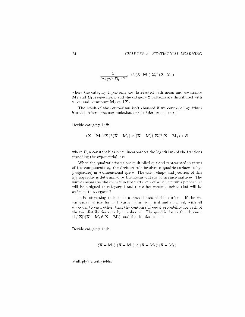
�� CHAPTER �� STATISTICAL LEARNING
�
�� �n��j��j���e�����X�M��
t���
� �X�M��
where the category � patterns are distributed with mean and covarianceM� and ��� respectively� and the category � patterns are distributed withmean and covarianceM� and ���
The result of the comparison isn�t changed if we compare logarithmsinstead� After some manipulation� our decision rule is then�
Decide category � i��
�X�M��t���
� �X�M�� � �X�M��t���
� �X�M�� #B
where B� a constant bias term� incorporates the logarithms of the fractionspreceding the exponential� etc�
When the quadratic forms are multiplied out and represented in termsof the components xi� the decision rule involves a quadric surface �a hyperquadric� in ndimensional space� The exact shape and position of thishyperquadric is determined by the means and the covariance matrices� Thesurface separates the space into two parts� one of which contains points thatwill be assigned to category � and the other contains points that will beassigned to category ��
It is interesting to look at a special case of this surface� If the covariance matrices for each category are identical and diagonal� with all�ii equal to each other� then the contours of equal probability for each ofthe two distributions are hyperspherical� The quadric forms then become���j�j��X�Mi�t�X�Mi�� and the decision rule is�
Decide category � i��
�X�M��t�X�M�� � �X�M��
t�X�M��
Multiplying out yields�

���� USING STATISTICAL DECISION THEORY ��
X�X � �X�M� �M��M� � X�X� �X�M� �M��M�
or �nally�
Decide category � i��
X�M� � X�M� � Constant
or
X��M� �M�� � Constant
where the constant depends on the lengths of the mean vectors�
We see that the optimal decision surface in this special case is a hyperplane� In fact� the hyperplane is perpendicular to the line joining the twomeans� The weights in a TLU implementation are equal to the di�erencein the mean vectors�
If the parameters �Mi��i� of the probability distributions of the categories are not known� there are various techniques for estimating them� andthen using those estimates in the decision rule� For example� if there are suf�cient training patterns� one can use sample means and sample covariancematrices� �Caution� the sample covariance matrix will be singular if thetraining patterns happen to lie on a subspace of the whole ndimensionalspace�as they certainly will� for example� if the number of training patterns is less than n��
���� Conditionally Independent Binary Components
Suppose the vectorX is a random variable having binary � ��� components�We continue to denote the two probability distributions by p�X j �� andp�X j ��� Further suppose that the components of these vectors are conditionally independent given the category� By conditional independence inthis case� we mean that the formulas for the distribution can be expandedas follows�
p�X j i� p�x� j i�p�x� j i� � � � p�xn j i�
for i �� �

� CHAPTER �� STATISTICAL LEARNING
Recall the minimumaverageloss decision rule�
Decide category � i��
��� j ��p�X j ��p��� ��� j ��p�X j ��p���
Assuming conditional independence of the components and that ��� j �� ��� j ��� we obtain�
Decide category � i��
p���p�x� j ��p�x� j �� � � � p�xn j �� � p�x� j ��p�x� j �� � � � p�xn j ��p���
or i��
p�x� j ��p�x� j �� � � � p�xn j ��
p�x� j ��p�x� j �� � � � p�xn j ���
p���
p���
or i��
logp�x� j ��
p�x� j ��# log
p�x� j ��
p�x� j ��# � � � # log
p�xn j ��
p�xn j ��# log
p���
p����
Let us de�ne values of the components of the distribution for speci�c valuesof their arguments� xi �
p�xi � j �� pi
p�xi j �� �� pi
p�xi � j �� qi
p�xi j �� �� qi
Now� we note that since xi can only assume the values of � or �
logp�xi j ��
p�xi j �� xi log
piqi# ��� xi� log
��� pi�
��� qi�
xi logpi��� qi�
qi��� pi�# log
��� pi�
��� qi�

���� LEARNING BELIEF NETWORKS ��
Substituting these expressions into our decision rule yields�
Decide category � i��
nXi �
xi logpi��� qi�
qi��� pi�#
nXi �
log��� pi�
��� qi�# log
p���
p����
We see that we can achieve this decision with a TLU with weight values asfollows�
wi logpi��� qi�
qi��� pi�
for i �� � � � � n� and
wn�� logp���
�� p���#
nXi �
log��� pi�
��� qi�
If we do not know the pi� qi and p���� we can use a sample of labeled trainingpatterns to estimate these parameters�
��� Learning Belief NetworksTo be added�
��� NearestNeighbor Methods
Another class of methods can be related to the statistical ones� These arecalled nearest�neighbor methods or� sometimes�memory�based methods� �Acollection of papers on this subject is in �Dasarathy� ������� Given a trainingset ! ofm labeled patterns� a nearestneighbor procedure decides that somenew pattern� X� belongs to the same category as do its closest neighborsin !� More precisely� a knearestneighbor method assigns a new pattern�X� to that category to which the plurality of its k closest neighbors belong�Using relatively large values of k decreases the chance that the decisionwill be unduly in�uenced by a noisy training pattern close to X� But largevalues of k also reduce the acuity of the method� The knearestneighbormethod can be thought of as estimating the values of the probabilities ofthe classes given X� Of course the denser are the points around X� and thelarger the value of k� the better the estimate�

�� CHAPTER �� STATISTICAL LEARNING
The distance metric used in nearestneighbor methods �for numerical attributes� can be simple Euclidean distance� That is� the distance between two patterns �x��� x��� � � � � x�n� and �x��� x��� � � � � x�n� isqPn
j ��x�j � x�j��� This distance measure is often modi�ed by scaling
the features so that the spread of attribute values along each dimension isapproximately the same� In that case� the distance between the two vectors
would beqPn
j � a�j �x�j � x�j��� where aj is the scale factor for dimension
j�
An example of a nearestneighbor decision problem is shown in Fig� ����In the �gure the class of a training pattern is indicated by the number nextto it�
k = 8X (a pattern to be classified)
1
1
1 11
111
2
1
2
222
2
2 2
2
33
3
3
3
3
33
3
training patternclass of training pattern
four patterns of category 1two patterns of category 2two patterns of category 3
plurality are in category 1, sodecide X is in category 1
Figure ���� An �NearestNeighbor DecisionSee�Baum� ����for theoreticalanalysis oferror rate as afunction of thenumber oftrainingpatterns forthe case inwhich pointsare randomlydistributed onthe surface of aunit sphereand underlyingfunction islinearlyseparable�
Nearestneighbor methods are memory intensive because a large number of training patterns must be stored to achieve good generalization� Since memory cost is now reasonably low� the method and itsderivatives have seen several practical applications� �See� for example��Moore� ����� Moore� et al�� ������ Also� the distance calculations requiredto �nd nearest neighbors can often be e�ciently computed by kd�tree methods �Friedman� et al�� ������
A theorem by Cover and Hart �Cover � Hart� ���� relates the performance of the �nearestneighbor method to the performance of a minimum

���� BIBLIOGRAPHICAL AND HISTORICAL REMARKS ��
probabilityoferror classi�er� As mentioned earlier� the minimumprobabilityoferror classi�er would assign a new patternX to that categorythat maximized p�i�p�X j i�� where p�i� is the a priori probability of category i� and p�X j i� is the probability �or probability density function� of Xgiven thatX belongs to category i� for categories i �� � � � � R� Suppose theprobability of error in classifying patterns of such a minimumprobabilityoferror classi�er is �� The CoverHart theorem states that under verymild conditions �having to do with the smoothness of probability densityfunctions� the probability of error� �nn� of a �nearestneighbor classi�er isbounded by�
� �nn �
��� �
R
R� �
� ��
where R is the number of categories� Also see�Aha� �����
��� Bibliographical and Historical RemarksTo be added�

� CHAPTER �� STATISTICAL LEARNING

Chapter �
Decision Trees
�� De�nitions
A decision tree �generally de�ned� is a tree whose internal nodes are tests�on input patterns� and whose leaf nodes are categories �of patterns�� Weshow an example in Fig� ��� A decision tree assigns a class number �oroutput� to an input pattern by �ltering the pattern down through the testsin the tree� Each test has mutually exclusive and exhaustive outcomes� Forexample� test T� in the tree of Fig� �� has three outcomes� the leftmostone assigns the input pattern to class �� the middle one sends the inputpattern down to test T�� and the rightmost one assigns the pattern toclass �� We follow the usual convention of depicting the leaf nodes by theclass number�� Note that in discussing decision trees we are not limited toimplementing Boolean functions�they are useful for general� categoricallyvalued functions�
There are several dimensions along which decision trees might di�er�
a� The tests might be multivariate �testing on several features of theinput at once� or univariate �testing on only one of the features��
b� The tests might have two outcomes or more than two� �If all of thetests have two outcomes� we have a binary decision tree��
�One of the researchers who has done a lot of work on learning decision trees is RossQuinlan� Quinlan distinguishes between classes and categories� He calls the subsets ofpatterns that lter down to each tip categories and subsets of patterns having the samelabel classes� In Quinlans terminology� our example tree has nine categories and threeclasses� We will not make this distinction� however� but will use the words �category�and �class� interchangeably to refer to what Quinlan calls �class��
��

�� CHAPTER �� DECISION TREES
T1
T2 T3
T4
T4
T4
31
3 2
1 2 3
2 1
Figure ��� A Decision Tree
c� The features or attributes might be categorical or numeric� �Binaryvalued ones can be regarded as either��
d� We might have two classes or more than two� If we have two classesand binary inputs� the tree implements a Boolean function� and iscalled a Boolean decision tree�
It is straightforward to represent the function implemented by a univariate Boolean decision tree in DNF form� The DNF form implementedby such a tree can be obtained by tracing down each path leading to a tipnode corresponding to an output value of �� forming the conjunction of thetests along this path� and then taking the disjunction of these conjunctions�We show an example in Fig� ��� In drawing univariate decision trees� eachnonleaf node is depicted by a single attribute� If the attribute has value in the input pattern� we branch left� if it has value �� we branch right�
The kDL class of Boolean functions can be implemented by a multivariate decision tree having the �highly unbalanced� form shown in Fig���� Each test� ci� is a term of size k or less� The vi all have values of or��

���� SUPERVISED LEARNINGOF UNIVARIATEDECISION TREES��
x3
x2 x4
x1
10
1
1
0 0
0
1
x3x2
x3x2
x3x4
x3x4x1 x3x4x1f = x3x2 + x3x4x1
1
00
1 0
Figure ��� A Decision Tree Implementing a DNF Function
�� Supervised Learning of Univariate Deci
sion Trees
Several systems for learning decision trees have been proposed� Prominent among these are ID� and its new version� C��� �Quinlan� ����Quinlan� ������ and CART �Breiman� et al�� ����� We discuss here onlybatch methods� although incremental ones have also been proposed�Utgo�� ������
���� Selecting the Type of Test
As usual� we have n features or attributes� If the attributes are binary� thetests are simply whether the attribute�s value is or �� If the attributesare categorical� but nonbinary� the tests might be formed by dividing theattribute values into mutually exclusive and exhaustive subsets� A decisiontree with such tests is shown in Fig� ��� If the attributes are numeric� thetests might involve �interval tests�� for example � xi �����

�� CHAPTER �� DECISION TREES
cq
cq-1
ci
1
vn
vn-1
vi
v1
Figure ��� A Decision Tree Implementing a Decision List
���� Using Uncertainty Reduction to Select Tests
The main problem in learning decision trees for the binaryattribute caseis selecting the order of the tests� For categorical and numeric attributes�we must also decide what the tests should be �besides selecting the order��Several techniques have been tried� the most popular one is at each stageto select that test that maximally reduces an entropylike measure�
We show how this technique works for the simple case of tests withbinary outcomes� Extension to multipleoutcome tests is straightforwardcomputationally but gives poor results because entropy is always decreasedby having more outcomes�
The entropy or uncertainty still remaining about the class of a pattern�knowing that it is in some set� !� of patterns is de�ned as�
H�!� �Xi
p�ij!� log� p�ij!�
where p�ij!� is the probability that a pattern drawn at random from !belongs to class i� and the summation is over all of the classes� We want toselect tests at each node such that as we travel down the decision tree� theuncertainty about the class of a pattern becomes less and less�

���� SUPERVISED LEARNINGOF UNIVARIATEDECISION TREES��
x3 = a, b, c, or d
{a, c}{b}
x1 = e, b, or d
{e,b}{d}
x4 = a, e, f, or g
{a, g} {e, f}
x2 = a, or g
{a} {g}
1
2 1
1 2
{d}
2
Figure ��� A Decision Tree with Categorical Attributes
Since we do not in general have the probabilities p�ij!�� we estimatethem by sample statistics� Although these estimates might be errorful�they are nevertheless useful in estimating uncertainties� Let &p�ij!� be thenumber of patterns in ! belonging to class i divided by the total numberof patterns in !� Then an estimate of the uncertainty is�
&H�!� �Xi
&p�ij!� log� &p�ij!�
For simplicity� from now on we�ll drop the �hats� and use sample statisticsas if they were real probabilities�
If we perform a test� T � having k possible outcomes on the patterns in!� we will create k subsets� !��!�� � � � �!k� Suppose that ni of the patternsin ! are in !i for i �� ���� k� �Some ni may be �� If we knew that Tapplied to a pattern in ! resulted in the jth outcome �that is� we knewthat the pattern was in !j�� the uncertainty about its class would be�
H�!j� �Xi
p�ij!j� log� p�ij!j�
and the reduction in uncertainty �beyond knowing only that the patternwas in !� would be�

� CHAPTER �� DECISION TREES
H�!��H�!j�
Of course we cannot say that the test T is guaranteed always to producethat amount of reduction in uncertainty because we don�t know that theresult of the test will be the jth outcome� But we can estimate the averageuncertainty over all the !j � by�
E�HT �!�� Xj
p�!j�H�!j�
where by HT �!� we mean the average uncertainty after performing test Ton the patterns in !� p�!j� is the probability that the test has outcome j�and the sum is taken from � to k� Again� we don�t know the probabilitiesp�!j�� but we can use sample values� The estimate &p�!j� of p�!j� is justthe number of those patterns in ! that have outcome j divided by the totalnumber of patterns in !� The average reduction in uncertainty achieved bytest T �applied to patterns in !� is then�
RT �!� H�!�� E�HT �!��
An important family of decision tree learning algorithms selects for theroot of the tree that test that gives maximum reduction of uncertainty� andthen applies this criterion recursively until some termination condition ismet �which we shall discuss in more detail later�� The uncertainty calculations are particularly simple when the tests have binary outcomes andwhen the attributes have binary values� We�ll give a simple example toillustrate how the test selection mechanism works in that case�
Suppose we want to use the uncertaintyreduction method to build adecision tree to classify the following patterns�
pattern class� � � � � � � �� � � �� � � � �� �� ��� � � ��� � �� ���� �� � ��� �� �� �

���� SUPERVISED LEARNINGOF UNIVARIATEDECISION TREES��
x1
x2
x3
The test x1
Figure ��� Eight Patterns to be Classi�ed by a Decision Tree
What single test� x�� x�� or x�� should be performed �rst� The illustrationin Fig� �� gives geometric intuition about the problem�
The initial uncertainty for the set� !� containing all eight points is�
H�!� ����� log������ ����� log������ ���
Next� we calculate the uncertainty reduction if we perform x� �rst� Thelefthand branch has only patterns belonging to class �we call them theset !l�� and the righthandbranch �!r� has two patterns in each class� So�the uncertainty of the lefthand branch is�
Hx��!l� ������ log������� � ��� log�� ���
And the uncertainty of the righthand branch is�
Hx��!r� ������ log������� ����� log������ �
Half of the patterns �go left� and half �go right� on test x�� Thus� theaverage uncertainty after performing the x� test is�
���Hx��!l� # ���Hx��!r� ��

�� CHAPTER �� DECISION TREES
Therefore the uncertainty reduction on ! achieved by x� is�
Rx��!� ���� �� ���
By similar calculations� we see that the test x� achieves exactly the sameuncertainty reduction� but x� achieves no reduction whatsoever� Thus� our�greedy� algorithm for selecting a �rst test would select either x� or x��Suppose x� is selected� The uncertaintyreduction procedure would selectx� as the next test� The decision tree that this procedure creates thusimplements the Boolean function� f x�x��See
�Quinlan� �����sect� � foranotherexample� ���� Non�Binary Attributes
If the attributes are nonbinary� we can still use the uncertaintyreductiontechnique to select tests� But now� in addition to selecting an attribute� wemust select a test on that attribute� Suppose for example that the valueof an attribute is a real number and that the test to be performed is toset a threshold and to test to see if the number is greater than or lessthan that threshold� In principle� given a set of labeled patterns� we canmeasure the uncertainty reduction for each test that is achieved by everypossible threshold �there are only a �nite number of thresholds that givedi�erent test results if there are only a �nite number of training patterns��Similarly� if an attribute is categorical �with a �nite number of categories��there are only a �nite number of mutually exclusive and exhaustive subsetsinto which the values of the attribute can be split� We can calculate theuncertainty reduction for each split�
�� Networks Equivalent to Decision Trees
Since univariate Boolean decision trees are implementations of DNF functions� they are also equivalent to twolayer� feedforward neural networks�We show an example in Fig� �� The decision tree at the left of the �gureimplements the same function as the network at the right of the �gure� Ofcourse� when implemented as a network� all of the features are evaluatedin parallel for any input pattern� whereas when implemented as a decisiontree only those features on the branch traveled down by the input patternneed to be evaluated� The decisiontree induction methods discussed in thischapter can thus be thought of as particular ways to establish the structureand the weight values for networks�

���� OVERFITTING AND EVALUATION ��
X
x1
x2
x3
x4
terms
-1
+1
disjunction
x3x2
x3x4x1
+1
-1
+1
f
1.5
0.5
x3
x2 x4
x1
10
1
1
0 0
0
1
x3x2
x3x2
x3x4
x3x4x1 x3x4x1
f = x3x2 + x3x4x1
1
00
10
Figure �� A Univariate Decision Tree and its Equivalent Network
Multivariate decision trees with linearly separable functions at eachnode can also be implemented by feedforward networks�in this case threelayer ones� We show an example in Fig� �� in which the linearly separablefunctions� each implemented by a TLU� are indicated by L�� L�� L�� andL�� Again� the �nal layer has �xed weights� but the weights in the �rst twolayers must be trained� Di�erent approaches to training procedures havebeen discussed by �Brent� ��� �� by �John� ������ and �for a special case�by �Marchand � Golea� ������
�� Over�tting and Evaluation
���� Over�tting
In supervised learning� we must choose a function to �t the training set fromamong a set of hypotheses� We have already showed that generalization isimpossible without bias� When we know a priori that the function we aretrying to guess belongs to a small subset of all possible functions� then�even with an incomplete set of training samples� it is possible to reduce thesubset of functions that are consistent with the training set su�ciently tomake useful guesses about the value of the function for inputs not in thetraining set� And� the larger the training set� the more likely it is that evena randomly selected consistent function will have appropriate outputs for

� CHAPTER �� DECISION TREES
L1
L2 L3
L4
10
1
1
0 0
0
1
1
00
10
X
L1
L2
L3
L4
conjunctions
L1L2
L1 L3 L4
−
+
++
disjunction
−
f
Figure ��� A Multivariate Decision Tree and its Equivalent Network
patterns not yet seen�
However� even with bias� if the training set is not su�ciently large compared with the size of the hypothesis space� there will still be too manyconsistent functions for us to make useful guesses� and generalization performance will be poor� When there are too many hypotheses that areconsistent with the training set� we say that we are over�tting the training data� Over�tting is a problem that we must address for all learningmethods�
Since a decision tree of su�cient size can implement any Boolean function there is a danger of over�tting�especially if the training set is small�That is� even if the decision tree is synthesized to classify all the membersof the training set correctly� it might perform poorly on new patterns thatwere not used to build the decision tree� Several techniques have been proposed to avoid over�tting� and we shall examine some of them here� Theymake use of methods for estimating how well a given decision tree mightgeneralize�methods we shall describe next�
���� Validation Methods
The most straightforward way to estimate how well a hypothesized function�such as a decision tree� performs on a test set is to test it on the testset" But� if we are comparing several learning systems �for example� ifwe are comparing di�erent decision trees� so that we can select the one

���� OVERFITTING AND EVALUATION ��
that performs the best on the test set� then such a comparison amounts to�training on the test data�� True� training on the test data enlarges thetraining set� with a consequent expected improvement in generalization� butthere is still the danger of over�tting if we are comparing several di�erentlearning systems� Another technique is to split the training set�using �say�twothirds for training and the other third for estimating generalizationperformance� But splitting reduces the size of the training set and therebyincreases the possibility of over�tting� We next describe some validationtechniques that attempt to avoid these problems�
Cross�Validation
In cross�validation� we divide the training set ! into K mutually exclusiveand exhaustive equalsized subsets� !�� � � � �!K � For each subset� !i� trainon the union of all of the other subsets� and empirically determine the errorrate� �i� on !i� �The error rate is the number of classi�cation errors madeon !i divided by the number of patterns in !i�� An estimate of the errorrate that can be expected on new patterns of a classi�er trained on all thepatterns in ! is then the average of the �i�
Leave�one�out Validation
Leave�one�out validation is the same as cross validation for the special casein which K equals the number of patterns in !� and each !i consists of asingle pattern� When testing on each !i� we simply note whether or nota mistake was made� We count the total number of mistakes and divideby K to get the estimated error rate� This type of validation is� of course�more expensive computationally� but useful when a more accurate estimateof the error rate for a classi�er is needed� Describe
�bootstrap�ping� also�Efron� �����
���� Avoiding Over�tting in Decision Trees
Near the tips of a decision tree there may be only a few patterns per node�For these nodes� we are selecting a test based on a very small sample� andthus we are likely to be over�tting� This problem can be dealt with by terminating the testgenerating procedure before all patterns are perfectly splitinto their separate categories� That is� a leaf node may contain patternsof more than one class� but we can decide in favor of the most numerousclass� This procedure will result in a few errors but often accepting a smallnumber of errors on the training set results in fewer errors on a testing set�
This behavior is illustrated in Fig� ���

�� CHAPTER �� DECISION TREES
(From Weiss, S., and Kulikowski, C., Computer Systems that Learn,Morgan Kaufmann, 1991)
training errors
validation errors
1 2 3 4 5 6 7 8 9
0.2
0.4
0.6
0.8
1.0
00
Error Rate
Number of TerminalNodes
Iris Data Decision Tree
Figure ��� Determining When Over�tting Begins
One can use crossvalidation techniques to determine when to stop splitting nodes� If the cross validation error increases as a consequence of a nodesplit� then don�t split� One has to be careful about when to stop� though�because under�tting usually leads to more errors on test sets than doesover�tting� There is a general rule that the lowest errorrate attainable bya subtree of a fully expanded tree can be no less than ��� of the error rateof the fully expanded tree �Weiss � Kulikowski� ����� page ����
Rather than stopping the growth of a decision tree� one might growit to its full size and then prune away leaf nodes and their ancestors until crossvalidation accuracy no longer increases� This techniqueis called post�pruning� Various techniques for pruning are discussed in�Weiss � Kulikowski� ������
���� Minimum�Description Length Methods
An important treegrowing and pruning technique is based on theminimum�description�length �MDL� principle� �MDL is an important ideathat extends beyond decisiontree methods �Rissanen� ������� The idea isthat the simplest decision tree that can predict the classes of the trainingpatterns is the best one� Consider the problem of transmitting just the

���� OVERFITTING AND EVALUATION ��
labels of a training set of patterns� assuming that the receiver of this information already has the ordered set of patterns� If there are m patterns�each labeled by one of R classes� one could transmit a list of m Rvaluednumbers� Assuming equally probable classes� this transmission would require m log�R bits� Or� one could transmit a decision tree that correctlylabelled all of the patterns� The number of bits that this transmission wouldrequire depends on the technique for encoding decision trees and on the sizeof the tree� If the tree is small and accurately classi�es all of the patterns� itmight be more economical to transmit the tree than to transmit the labelsdirectly� In between these extremes� we might transmit a tree plus a list oflabels of all the patterns that the tree misclassi�es�
In general� the number of bits �or description length of the binary encoded message� is t # d� where t is the length of the message required totransmit the tree� and d is the length of the message required to transmitthe labels of the patterns misclassi�ed by the tree� In a sense� that tree associated with the smallest value of t#d is the best or most economical tree�The MDL method is one way of adhering to the Occam�s razor principle�
Quinlan and Rivest �Quinlan � Rivest� ����� have proposed techniquesfor encoding decision trees and lists of exception labels and for calculatingthe description length �t# d� of these trees and labels� They then use thedescription length as a measure of quality of a tree in two ways�
a� In growing a tree� they use the reduction in description length toselect tests �instead of reduction in uncertainty��
b� In pruning a tree after it has been grown to zero error� they pruneaway those nodes �starting at the tips� that achieve a decrease in thedescription length�
These techniques compare favorably with the uncertaintyreductionmethod�although they are quite sensitive to the coding schemes used�
��� Noise in Data
Noise in the data means that one must inevitably accept some numberof errors�depending on the noise level� Refusal to tolerate errors on thetraining set when there is noise leads to the problem of ��tting the noise��Dealing with noise� then� requires accepting some errors at the leaf nodesjust as does the fact that there are a small number of patterns at leaf nodes�

�� CHAPTER �� DECISION TREES
�� The Problem of Replicated Subtrees
Decision trees are not the most economical means of implementing someBoolean functions� Consider� for example� the function f x�x� # x�x��A decision tree for this function is shown in Fig� ��� Notice the replicatedsubtrees shown circled� The DNFform equivalent to the function implemented by this decision tree is f x�x� # x�x�x�x� # x�x�x�� This DNFform is nonminimal �in the number of disjunctions� and is equivalent tof x�x� # x�x��
x1
x3 x2
10
x4
0 1
x3
0x4
0 1
Figure ��� A Decision Tree with Subtree Replication
The need for replication means that it takes longer to learn the treeand that subtrees replicated further down the tree must be learned using asmaller training subset� This problem is sometimes called the fragmentationproblem�
Several approaches might be suggested for dealing with fragmentation� One is to attempt to build a decision graph instead of a tree�Oliver� Dowe� � Wallace� ����� Kohavi� ������ A decision graph that implements the same decisions as that of the decision tree of Fig� �� is shownin Fig� �� �
Another approach is to use multivariate �rather than univariate tests ateach node�� In our example of learning f x�x� # x�x�� if we had a test

���� THE PROBLEM OF REPLICATED SUBTREES ��
x1
x3
x2
1
0x4
0 1
Figure �� � A Decision Graph
for x�x� and a test for x�x�� the decision tree could be much simpli�ed�as shown in Fig� ���� Several researchers have proposed techniques forlearning decision trees in which the tests at each node are linearly separablefunctions� �John� ����� gives a nice overview �with several citations� oflearning such linear discriminant trees and presents a method based on�soft entropy��
A third method for dealing with the replicated subtree problem involvesextracting propositional �rules� from the decision tree� The rules will haveas antecedents the conjunctions that lead down to the leaf nodes� and asconsequents the name of the class at the corresponding leaf node� An example rule from the tree with the repeating subtree of our example wouldbe� x� � �x� � x� � x� � �� Quinlan �Quinlan� ����� discusses methodsfor reducing a set of rules to a simpler set by �� eliminating from the antecedent of each rule any �unnecessary� conjuncts� and then �� eliminating�unnecessary� rules� A conjunct or rule is determined to be unnecessaryif its elimination has little e�ect on classi�cation accuracy�as determinedby a chisquare test� for example� After a rule set is processed� it might bethe case that more than one rule is �active� for any given pattern� and caremust be taken that the active rules do not con�ict in their decision aboutthe class of a pattern�

� CHAPTER �� DECISION TREES
x1x2
1
0
x3x4
1
Figure ���� A Multivariate Decision Tree
� The Problem of Missing AttributesTo be added�
�� Comparisons
Several experimenters have compared decisiontree� neuralnet� andnearestneighbor classi�ers on a wide variety of problems� For acomparison of neural nets versus decision trees� for example� see�Dietterich� et al�� ��� � Shavlik� Mooney� � Towell� ����� Quinlan� ������In their StatLog project� �Taylor� Michie� � Spiegalhalter� ����� give thorough comparisons of several machine learning algorithms on several di�erent types of problems� There seems to be no single type of classi�er that isbest for all problems� And� there do not seem to be any general conclusionsthat would enable one to say which classi�er method is best for which sortsof classi�cation problems� although �Quinlan� ����� does provide some intuition about properties of problems that might render them ill suited fordecision trees� on the one hand� or backpropagation� on the other�
� Bibliographical and Historical RemarksTo be added�

Chapter �
Inductive Logic
Programming
There are many di�erent representational forms for functions of input variables� So far� we have seen �Boolean� algebraic expressions� decision trees�and neural networks� plus other computational mechanisms such as techniques for computing nearest neighbors� Of course� the representationmostimportant in computer science is a computer program� For example� a Lisppredicate of binaryvalued inputs computes a Boolean function of those inputs� Similarly� a logic program �whose ordinary application is to computebindings for variables� can also be used simply to decide whether or nota predicate has value True �T� or False �F�� For example� the Booleanexclusiveor �odd parity� function of two variables can be computed by thefollowing logic program�
Parity�x�y� �� True�x�� � True�y�
�� True�y�� � True�x�
We follow Prolog syntax �see� for example� �Mueller � Page� ������� exceptthat our convention is to write variables as strings beginning with lowercase letters and predicates as strings beginning with uppercase letters� Theunary function �True� returns T if and only if the value of its argument isT � �We now think of Boolean functions and arguments as having values ofT and F instead of and ��� Programs will be written in �typewriter�font�
��

�� CHAPTER �� INDUCTIVE LOGIC PROGRAMMING
In this chapter� we consider the matter of learning logic programs givena set of variable values for which the logic program should return T �thepositive instances� and a set of variable values for which it should return F�the negative instances�� The subspecialty of machine learning that dealswith learning logic programs is called inductive logic programming �ILP��Lavra�c � D�zeroski� ������ As with any learning problem� this one can bequite complex and intractably di�cult unless we constrain it with biases ofsome sort� In ILP� there are a variety of possible biases �called language bi�ases�� One might restrict the program to Horn clauses� not allow recursion�not allow functions� and so on�
As an example of an ILP problem� suppose we are trying to induce afunction Nonstop�x�y�� that is to have value T for pairs of cities connectedby a nonstop air �ight and F for all other pairs of cities� We are given atraining set consisting of positive and negative examples� As positive examples� we might have �A�B�� �A� A��� and some other pairs� as negativeexamples� we might have �A�� A��� and some other pairs� In ILP� we usually have additional information about the examples� called �backgroundknowledge�� In our air�ight problem� the background information mightbe such ground facts as Hub�A�� Hub�B�� Satellite�A��A�� plus others��Hub�A� is intended to mean that the city denoted by A is a hub city� andSatellite�A��A� is intended to mean that the city denoted by A� is asatellite of the city denoted by A�� From these training facts� we want toinduce a program Nonstop�x�y�� written in terms of the background relations Hub and Satellite� that has value T for all the positive instancesand has value F for all the negative instances� Depending on the exact setof examples� we might induce the program�
Nonstop�x�y� �� Hub�x�� Hub�y�
�� Satellite�x�y�
�� Satellite�y�x�
which would have value T if both of the two cities were hub cities or ifone were a satellite of the other� As with other learning problems� wewant the induced program to generalize well� that is� if presented witharguments not represented in the training set �but for which we have theneeded background knowledge�� we would like the function to guess well�

���� NOTATION AND DEFINITIONS ��
��� Notation and De�nitions
In evaluating logic programs in ILP� we implicitly append the backgroundfacts to the program and adopt the usual convention that a program hasvalue T for a set of inputs if and only if the program interpreter returnsT when actually running the program �with background facts appended�on those inputs� otherwise it has value F � Using the given backgroundfacts� the program above would return T for input �A� A��� for example�If a logic program� � returns T for a set of arguments X� we say thatthe program covers the arguments and write covers� �X�� Following ourterminology introduced in connection with version spaces� we will say thata program is su�cient if it covers all of the positive instances and thatit is necessary if it does not cover any of the negative instances� �Thatis� a program implements a su�cient condition that a training instanceis positive if it covers all of the positive training instances� it implementsa necessary condition if it covers none of the negative instances�� In thenoiseless case� we want to induce a program that is both su�cient andnecessary� in which case we will call it consistent� With imperfect �noisy�training sets� we might relax this criterion and settle for a program thatcovers all but some fraction of the positive instances while allowing it tocover some fraction of the negative instances� We illustrate these de�nitionsschematically in Fig� ����
−
−
−−
−
−−
π1 is a necessary program
π2 is a sufficient program
π3 is a consistent program
+
+
++
++
+
++
+
−−
A positive instance covered by π2 and π3
Figure ���� Su�cient� Necessary� and Consistent Programs
As in version spaces� if a program is su�cient but not necessary it can be

� CHAPTER �� INDUCTIVE LOGIC PROGRAMMING
made to cover fewer examples by specializing it� Conversely� if it is necessarybut not su�cient� it can be made to cover more examples by generalizingit� Suppose we are attempting to induce a logic program to compute therelation �� The most general logic program� which is certainly su�cient�is the one that has value T for all inputs� namely a single clause with anempty body� �� �� �� which is called a fact in Prolog� The most speciallogic program� which is certainly necessary� is the one that has value F forall inputs� namely �� �� F �� Two of the many di�erent ways to search fora consistent logic program are� �� start with �� �� � and specialize untilthe program is consistent� or �� start with �� �� F � and generalize untilthe program is consistent� We will be discussing a method that starts with�� �� �� specializes until the program is necessary �but might no longer besu�cient�� then reachieves su�ciency in stages by generalizing�ensuringwithin each stage that the program remains necessary �by specializing��
��� A Generic ILP Algorithm
Since the primary operators in our search for a consistent program arespecialization and generalization� we must next discuss those operations�There are three major ways in which a logic program might be generalized�
a� Replace some terms in a program clause by variables� �Readers familiar with substitutions in the predicate calculus will note that thisprocess is the inverse of substitution��
b� Remove literals from the body of a clause�
c� Add a clause to the program
Analogously� there are three ways in which a logic program might be specialized�
a� Replace some variables in a program clause by terms �a substitution��
b� Add literals to the body of a clause�
c� Remove a clause from the program
We will be presenting an ILP learning method that adds clauses to a program when generalizing and that adds literals to the body of a clause whenspecializing� When we add a clause� we will always add the clause �� �� �

���� A GENERIC ILP ALGORITHM � �
and then specialize it by adding literals to the body� Thus� we need onlydescribe the process for adding literals�
Clauses can be partially ordered by the specialization relation� In general� clause c� is more special than clause c� if c� j c�� A special case�which is what we use here� is that a clause c� is more special than a clausec� if the set of literals in the body of c� is a subset of those in c�� Thisordering relation can be used in a structure of partially ordered clauses�called the re�nement graph� that is similar to a version space� Clause c� isan immediate successor of clause c� in this graph if and only if clause c�can be obtained from clause c� by adding a literal to the body of c�� Are�nement graph then tells us the ways in which we can specialize a clauseby adding a literal to it�
Of course there are unlimited possible literals we might add to the bodyof a clause� Practical ILP systems restrict the literals in various ways�Typical allowed additions are�
a� Literals used in the background knowledge�
b� Literals whose arguments are a subset of those in the head of theclause�
c� Literals that introduce a new distinct variable di�erent from those inthe head of the clause�
d� A literal that equates a variable in the head of the clause with anothersuch variable or with a term mentioned in the background knowledge��This possibility is equivalent to forming a specialization by makinga substitution��
e� A literal that is the same �except for its arguments� as that in thehead of the clause� �This possibility admits recursive programs� whichare disallowed in some systems��
We can illustrate these possibilities using our air�ight example� Westart with the program �Nonstop�x�y� �� �� The literals used in thebackground knowledge are Hub and Satellite� Thus the literals that wemight consider adding are�
Hub�x�
Hub�y�
Hub�z�
Satellite�x�y�

� � CHAPTER �� INDUCTIVE LOGIC PROGRAMMING
Satellite�y�x�
Satellite�x�z�
Satellite�z�y�
�x � y�
�If recursive programs are allowed� we could also add the literalsNonstop�x�z� and Nonstop�z�y��� These possibilities are among those illustrated in the re�nement graph shown in Fig� ���� Whatever restrictionson additional literals are imposed� they are all syntactic ones from whichthe successors in the re�nement graph are easily computed� ILP programsthat follow the approach we are discussing �of specializing clauses by addinga literal� thus have well de�ned methods of computing the possible literalsto add to a clause�
Nonstop(x,y) :-
Nonstop(x,y) :- Hub(x)
Nonstop(x,y) :- Satellite(x,y)
Nonstop(x,y) :- (x = y)
. . .
. . .
. . . . . .
Nonstop(x,y) :- Hub(x), Hub(y)
. . .
. . .
. . .
Figure ���� Part of a Re�nement Graph
Now we are ready to write down a simple generic algorithm for inducinga logic program� for inducing a relation �� We are given a training set�! of argument sets some known to be in the relation � and some not in

���� AN EXAMPLE � �
�� !� are the positive instances� and !� are the negative instances� Thealgorithm has an outer loop in which it successively adds clauses to make more and more su�cient� It has an inner loop for constructing a clause�c� that is more and more necessary and in which it refers only to a subset�!cur� of the training instances� �The positive instances in !cur will bedenoted by !�cur� and the negative ones by !
�cur�� The algorithm is also
given background relations and the means for adding literals to a clause�It uses a logic program interpreter to compute whether or not the programit is inducing covers training instances� The algorithm can be written asfollows�
Generic ILP Algorithm
�Adapted from �Lavra�c � D�zeroski� ����� p� ���
Initialize !cur � !�Initialize � empty set of clauses�repeat �The outer loop works to make su�cient��
Initialize c � � � � �repeat �The inner loop makes c necessary��
Select a literal l to add to c� �This is a nondeterministic choice point��Assign c � c� l�
until c is necessary� �That is� until c covers no negative instances in !cur��Assign � � c� �We add the clause c to the program��Assign !cur � !cur � �the positive instances in !cur covered by ��
until is su�cient�
�The termination tests for the inner and outer loops can be relaxed asappropriate for the case of noisy instances��
��� An Example
We illustrate how the algorithmworks by returning to our example of airline�ights� Consider the portion of an airline route map� shown in Fig� ����Cities A� B� and C are �hub� cities� and we know that there are nonstop�ights between all hub cities �even those not shown on this portion of theroute map�� The other cities are �satellites� of one of the hubs� and we knowthat there are nonstop �ights between each satellite city and its hub� Thelearning program is given a set of positive instances� !�� of pairs of citiesbetween which there are nonstop �ights and a set of negative instances� !��

� � CHAPTER �� INDUCTIVE LOGIC PROGRAMMING
of pairs of cities between which there are not nonstop �ights� !� containsjust the pairs�
f� A�B ��� A�C ��� B�C ��� B�A ��� C�A ��� C�B ��
� A�A� ��� A�A� ��� A�� A ��� A�� A ��� B�B� ��� B�B� ��
� B�� B ��� B�� B ��� C�C� ��� C�C� ��� C�� C ��� C�� C �g
For our example� we will assume that !� contains all those pairs of citiesshown in Fig� ��� that are not in !� �a type of closed�world assumption��These are�
f� A�B� ��� A�B� ��� A�C� ��� A�C� ��� B�C� ��� B�C� ��
� B�A� ��� B�A� ��� C�A� ��� C�A� ��� C�B� ��� C�B� ��
� B�� A ��� B�� A ��� C�� A ��� C�� A ��� C�� B ��� C�� B ��
� A�� B ��� A�� B ��� A�� C ��� A�� C ��� B�� C ��� B�� C �g
There may be other cities not shown on this map� so the training set doesnot necessarily exhaust all the cities�
A
B
C
C1
C2
B1 B2
A1
A2
Figure ���� Part of an Airline Route Map

���� AN EXAMPLE � �
We want the learning program to induce a program for computing thevalue of the relation Nonstop� The training set� !� can be thought of as apartial description of this relation in extensional form�it explicitly namessome pairs in the relation and some pairs not in the relation� We desire tolearn the Nonstop relation as a logic program in terms of the backgroundrelations� Hub and Satellite� which are also given in extensional form�Doing so will give us a more compact� intensional� description of the relation� and this description could well generalize usefully to other cities notmentioned in the map�
We assume the learning program has the following extensional de�nitions of the relations Hub and Satellite�
Hub
f� A ��� B ��� C �g
All other cities mentioned in the map are assumed not in the relation Hub�We will use the notation Hub�x� to express that the city named x is in therelation Hub�
Satellite
f� A�� A���� A�� A ��� B�� B ��� B�� B ��� C�� C ��� C�� C �g
All other pairs of cities mentioned in the map are not in the relationSatellite� We will use the notation Satellite�x�y� to express that thepair � x� y � is in the relation Satellite�
Knowing that the predicate Nonstop is a twoplace predicate� the innerloop of our algorithm initializes the �rst clause to Nonstop�x�y� �� �This clause is not necessary because it covers all the negative examples�since it covers all examples�� So we must add a literal to its �empty� body�Suppose �selecting a literal from the re�nement graph� the algorithm addsHub�x�� The following positive instances in ! are covered by Nonstop�x�y��� Hub�x��

� CHAPTER �� INDUCTIVE LOGIC PROGRAMMING
f� A�B ��� A�C ��� B�C ��� B�A ��� C�A ��� C�B ��
� A�A� ��� A�A� ��� B�B� ��� B�B� ��� C�C� ��� C�C� �g
To compute this covering� we interpret the logic program Nonstop�x�y� ��
Hub�x� for all pairs of cities in !� using the pairs given in the backgroundrelation Hub as ground facts� The following negative instances are alsocovered�
f� A�B� ��� A�B� ��� A�C� ��� A�C� ��� C�A� ��� C�A� ��
� C�B� ��� C�B� ��� B�A� ��� B�A� ��� B�C� ��� B�C� �g
Thus� the clause is not yet necessary and another literal must be added�Suppose we next add Hub�y�� The following positive instances are coveredby Nonstop�x�y� �� Hub�x�� Hub�y��
f� A�B ��� A�C ��� B�C ��� B�A ��� C�A ��� C�B �g
There are no longer any negative instances in ! covered so the clauseNonstop�x�y� �� Hub�x�� Hub�y� is necessary� and we can terminate the�rst pass through the inner loop�
But the program� � consisting of just this clause is not su�cient� Thesepositive instances are not covered by the clause�
f� A�A� ��� A�A� ��� A�� A ��� A�� A ��� B�B� ��� B�B� ��
� B�� B ��� B�� B ��� C�C� ��� C�C� ��� C�� C ��� C�� C �g
The positive instances that were covered by Nonstop�x�y� �� Hub�x��
Hub�y� are removed from ! to form the !cur to be used in the next passthrough the inner loop� !cur consists of all the negative instances in ! plusthe positive instances �listed above� that are not yet covered� In order toattempt to cover them� the inner loop creates another clause c� initially setto Nonstop�x�y� �� � This clause covers all the negative instances� andso we must add literals to make it necessary� Suppose we add the literalSatellite�x�y�� The clause Nonstop�x�y� �� Satellite�x�y� coversno negative instances� so it is necessary� It does cover the following positiveinstances in !cur�

���� INDUCING RECURSIVE PROGRAMS � �
f� A�� A ��� A�� A ��� B�� B ��� B�� B ��� C�� C ��� C�� C �g
These instances are removed from !cur for the next pass through the innerloop� The program now contains two clauses�
Nonstop�x�y� �� Hub�x�� Hub�y�
�� Satellite�x�y�
This program is not yet su�cient since it does not cover the followingpositive instances�
f� A�A� ��� A�A� ��� B�B� ��� B�B� ��� C�C� ��� C�C� �g
During the next pass through the inner loop� we add the clauseNonstop�x�y� �� Satellite�y�x�� This clause is necessary� and sincethe program containing all three clauses is now su�cient� the procedureterminates with�
Nonstop�x�y� �� Hub�x�� Hub�y�
�� Satellite�x�y�
�� Satellite�y�x�
Since each clause is necessary� and the whole program is su�cient� theprogram is also consistent with all instances of the training set� Note thatthis program can be applied �perhaps with good generalization� to othercities besides those in our partial map�so long as we can evaluate therelations Hub and Satellite for these other cities� In the next section� weshow how the technique can be extended to use recursion on the relationwe are inducing� With that extension� the method can be used to inducemore general logic programs�
��� Inducing Recursive Programs
To induce a recursive program� we allow the addition of a literal having thesame predicate letter as that in the head of the clause� Various mechanismsmust be used to ensure that such a program will terminate� one such is tomake sure that the new literal has di�erent variables than those in the

� � CHAPTER �� INDUCTIVE LOGIC PROGRAMMING
head literal� The process is best illustrated with another example� Ourexample continues the one using the airline map� but we make the mapsomewhat simpler in order to reduce the size of the extensional relationsused� Consider the map shown in Fig� ���� Again� B and C are hub cities�B� and B are satellites of B� C� and C are satellites of C� We haveintroduced two new cities� B and C� No �ights exist between these citiesand any other cities�perhaps there are only bus routes as shown by thegrey lines in the map�
B
C
C1
C2
B1B2
B3
C3
Figure ���� Another Airline Route Map
We now seek to learn a program for Canfly�x�y� that covers only thosepairs of cities that can be reached by one or more nonstop �ights� Therelation Canfly is satis�ed by the following pairs of postive instances�
f� B�� B ��� B�� B� ��� B�� C ��� B�� C� ��� B�� C� ��
� B�B� ��� B�� B� ��� C�B� ��� C�� B� ��� C�� B� ��
� B�� B ��� B�� C ��� B�� C� ��� B�� C� ��� B�B� ��
� C�B� ��� C�� B� ��� C�� B� ��� B�C ��� B�C� ��
� B�C� ��� C�B ��� C�� B ��� C�� B ��� C�C� ��
� C�C� ��� C�� C ��� C�� C ��� C�� C� ��� C�� C� �g

���� INDUCING RECURSIVE PROGRAMS � �
Using a closedworld assumption on our map� we take the negative instancesof Canfly to be�
f� B�� B� ��� B�� B ��� B�� B� ��� B�� C ��� B�� C� ��
� B�� C� ��� B�� C� ��� B�� B� ��� B�B� ��� B�� B� ��
� C�B� ��� C�� B� ��� C�� B� ��� C�� B� ��� C�� B� ��
� C�� B ��� C�� B� ��� C�� C ��� C�� C� ��� C�� C� ��
� B�� C� ��� B�C� ��� B�� C� ��� C�C� ��� C�� C� ��
� C�� C� �g
We will induce Canfly�x�y� using the extensionally de�ned backgroundrelation Nonstop given earlier �modi�ed as required for our reduced airlinemap� and Canfly itself �recursively��
As before� we start with the empty program and proceed to the innerloop to construct a clause that is necessary� Suppose that the inner loopadds the background literal Nonstop�x�y�� The clause Canfly�x�y� ��
Nonstop�x�y� is necessary� it covers no negative instances� But it is notsu�cient because it does not cover the following positive instances�
f� B�� B� ��� B�� C ��� B�� C� ��� B�� C� ��� B�� B� ��
� C�B� ��� C�� B� ��� C�� B� ��� B�� C ��� B�� C� ��
� B�� C� ��� C�B� ��� C�� B� ��� C�� B� ��� B�C� ��
� B�C� ��� C�� B ��� C�� B ��� C�� C� ��� C�� C� �g
Thus� we must add another clause to the program� In the inner loop� we �rstcreate the clause Canfly�x�y� �� Nonstop�x�z� which introduces the newvariable z� We digress brie�y to describe how a program containing a clausewith unbound variables in its body is interpreted� Suppose we try to interpret it for the positive instance Canfly�B��B��� The interpreter attemptsto establish Nonstop�B��z� for some z� Since Nonstop�B�� B�� for example� is a background fact� the interpreter returns T�which means that theinstance � B�� B� � is covered� Suppose now� we attempt to interpret theclause for the negative instance Canfly�B��B�� The interpreter attempts toestablish Nonstop�B��z� for some z� There are no background facts thatmatch� so the clause does not cover � B�� B �� Using the interpreter� wesee that the clause Canfly�x�y� �� Nonstop�x�z� covers all of the positive instances not already covered by the �rst clause� but it also coversmany negative instances such as � B�� B� �� and � B�B� �� So the inner

�� CHAPTER �� INDUCTIVE LOGIC PROGRAMMING
loop must add another literal� This time� suppose it adds Canfly�z�y�to yield the clause Canfly�x�y� �� Nonstop�x�z�� Canfly�z�y�� Thisclause is necessary� no negative instances are covered� The program is nowsu�cient and consistent� it is�
Canfly�x�y� �� Nonstop�x�y�
�� Nonstop�x�z�� Canfly�z�y�
��� Choosing Literals to Add
One of the �rst practical ILP systems was Quinlan�s FOIL �Quinlan� ��� ��A major problem involves deciding how to select a literal to add in theinner loop �from among the literals that are allowed�� In FOIL� Quinlansuggested that candidate literals can be compared using an informationlike measure�similar to the measures used in inducing decision trees� Ameasure that gives the same comparison as does Quinlan�s is based on theamount by which adding a literal increases the odds that an instance drawnat random from those covered by the new clause is a positive instancebeyond what these odds were before adding the literal�
Let p be an estimate of the probability that an instance drawn at random from those covered by a clause before adding the literal is a positive instance� That is� p �number of positive instances covered by theclause���total number of instances covered by the clause�� It is convenientto express this probability in �odds form�� The odds� o� that a covered instance is positive is de�ned to be o p���� p�� Expressing the probabilityin terms of the odds� we obtain p o��� # o��
After selecting a literal� l� to add to a clause� some of the instancespreviously covered are still covered� some of these are positive and some arenegative� Let pl denote the probability that an instance drawn at randomfrom the instances covered by the new clause �with l added� is positive�The odds will be denoted by ol� We want to select a literal� l� that givesmaximal increase in these odds� That is� if we de�ne �l ol�o� we want aliteral that gives a high value of �l� Specializing the clause in such a waythat it fails to cover many of the negative instances previously covered butstill covers most of the positive instances previously covered will result ina high value of �l� �It turns out that the value of Quinlan�s informationtheoretic measure increases monotonically with �l� so we could just as welluse the latter instead��

���� RELATIONSHIPSBETWEEN ILP ANDDECISION TREE INDUCTION���
Besides �nding a literal with a high value of �l� Quinlan�s FOIL systemalso restricts the choice to literals that�
a� contain at least one variable that has already been used�
b� place further restrictions on the variables if the literal selected hasthe same predicate letter as the literal being induced �in order to preventin�nite recursion�� and
c� survive a pruning test based on the values of �l for those literalsselected so far�
We refer the reader to Quinlan�s paper for further discussion of these points�Quinlan also discusses postprocessing pruning methods and presents experimental results of the method applied to learning recursive relations onlists� on learning rules for chess endgames and for the card game Eleusis� and for some other standard tasks mentioned in the machine learningliterature�
The reader should also refer to �Pazzani � Kibler� �����Lavra�c � D�zeroski� ����� Muggleton� ����� Muggleton� ������ Discuss
preprocessing�postprocessing�bottom�upmethods� andLINUS�
�� Relationships Between ILP and Deci
sion Tree Induction
The generic ILP algorithm can also be understood as a type of decision treeinduction� Recall the problem of inducing decision trees when the values ofattributes are categorical� When splitting on a single variable� the split ateach node involves asking to which of several mutually exclusive and exhaustive subsets the value of a variable belongs� For example� if a node testedthe variable xi� and if xi could have values drawn from fA�B�C�D�E� Fg�then one possible split �among many� might be according to whether thevalue of xi had as value one of fA�B�Cg or one of fD�E�Fg�
It is also possible to make a multivariate split�testing the values oftwo or more variables at a time� With categorical variables� an nvariablesplit would be based on which of several nary relations the values of thevariables satis�ed� For example� if a node tested the variables xi and xj �and if xi and xj both could have values drawn from fA�B�C�D�E� Fg� thenone possible binary split �among many� might be according to whether ornot � xi� xj � satis�ed the relation f� A�C ��� C�D �g� �Note thatour subset method of forming singlevariable splits could equivalently havebeen framed using �ary relations�which are usually called properties��
In this framework� the ILP problem is as follows� We are given a trainingset� !� of positively and negatively labeled patterns whose components are

��� CHAPTER �� INDUCTIVE LOGIC PROGRAMMING
drawn from a set of variables fx� y� z� � � �g� The positively labeled patternsin ! form an extensional de�nition of a relation� R� We are also given background relations� R�� � � � � Rk� on various subsets of these variables� �Thatis� we are given sets of tuples that are in these relations�� We desire toconstruct an intensional de�nition of R in terms of the R�� � � � � Rk� suchthat all of the positively labeled patterns in ! are satis�ed by R and noneof the negatively labeled patterns are� The intensional de�nition will bein terms of a logic program in which the relation R is the head of a set ofclauses whose bodies involve the background relations�
The generic ILP algorithm can be understood as decision tree induction�where each node of the decision tree is itself a subdecision tree� and eachsubdecision tree consists of nodes that make binary splits on several variables using the background relations� Ri� Thus we will speak of a topleveldecision tree and various subdecision trees� �Actually� our decision treeswill be decision lists�a special case of decision trees� but we will refer tothem as trees in our discussions��
In broad outline� the method for inducing an intensional version of therelation R is illustrated by considering the decision tree shown in Fig� ����In this diagram� the patterns in ! are �rst �ltered through the decisiontree in toplevel node �� The background relation R� is satis�ed by someof these patterns� these are �ltered to the right �to relation R��� and therest are �ltered to the left �more on what happens to these later�� Rightgoing patterns are �ltered through a sequence of relational tests until onlypositively labeled patterns satisfy the last relation�in this caseR�� That is�the subset of patterns satisfying all the relations� R�� R�� and R� containsonly positive instances from !� �We might say that this combination oftests is necessary� They correspond to the clause created in the �rst passthrough the inner loop of the generic ILP algorithm�� Let us call the subsetof patterns satisfying these relations� !�� these satisfy Node � at the toplevel� All other patterns� that is f! � !�g !� are �ltered to the left byNode ��
!� is then �ltered by toplevel Node � in much the same manner� so thatNode � is satis�ed only by the positively labeled samples in !�� We continue�ltering through toplevel nodes until only the negatively labeled patternsfail to satisfy a top node� In our example� !� contains only negativelylabeled patterns and the union of !� and !� contains all the positivelylabeled patterns� The relation� R� that distinguishes positive from negativepatterns in ! is then given in terms of the following logic program�
R �� R�� R�� R�
�� R� R

���� RELATIONSHIPSBETWEEN ILP ANDDECISION TREE INDUCTION���
R1
R2
R3
T
T
T
F
F
F
T
F
R4
R5
T
T
F
F
TF
Ξ
Ξ1
Ξ2 = Ξ − Ξ1
Ξ3Ξ4= Ξ2 − Ξ3
Node 1
Node 2
(only positiveinstancessatisfy all threetests)
(only positivelinstances satisfythese two tests)
(only negativeinstances)
Figure ���� A Decision Tree for ILP
If we apply this sort of decisiontree induction procedure to the problemof generating a logic program for the relation Nonstop �refer to Fig� �����we obtain the decision tree shown in Fig� ��� The logic program resultingfrom this decision tree is the same as that produced by the generic ILPalgorithm�
In setting up the problem� the training set� ! can be expressed as aset of �dimensional vectors with components x and y� The values of thesecomponents range over the cities fA�B�C�A�� A�� B�� B�� C�� C�g except�for simplicity� we do not allow patterns in which x and y have the samevalue� As before� the relation� Nonstop� contains the following pairs ofcities� which are the positive instances�
f� A�B ��� A�C ��� B�C ��� B�A ��� C�A ��� C�B ��
� A�A� ��� A�A� ��� A�� A ��� A�� A ��� B�B� ��� B�B� ��
� B�� B ��� B�� B ��� C�C� ��� C�C� ��� C�� C ��� C�� C �g

��� CHAPTER �� INDUCTIVE LOGIC PROGRAMMING
All other pairs of cities named in the map of Fig� ��� �using the closedworld assumption� are not in the relation Nonstop and thus are negativeinstances�
Because the values of x and y are categorical� decisiontree inductionwould be a very di�cult task�involving as it does the need to invent relations on x and y to be used as tests� But with the background relations� Ri
�in this case Hub and Satellite�� the problem is made much easier� Weselect these relations in the same way that we select literals� from amongthe available tests� we make a selection based on which leads to the largestvalue of �Ri
�
��� Bibliographical and Historical RemarksTo be added�

���� BIBLIOGRAPHICAL AND HISTORICAL REMARKS ���
Hub(x) TF
ΞNode 1(top level)
{<A,B>, <A,C>,<B,C>, <B,A>,<C,A>, <C,B>}
Hub(y)T
TFNode 2
(top level)
Satellite(x,y)F T
T{<A1,A>, <A2,A>, <B1,B>,<B2,B>, <C1,C>, <C2,C>}
F
{<A,A1>, <A,A2>,<B,B1>,<B,B2>, <C,C1>, <C,C2>}
Satellite(y,x)F
F
T
Node 3(top level)
T
{Only negative instances}
(Only positive instances)
(Only positive instances)
(Only positive instances)
F
Figure ��� A Decision Tree for the Airline Route Problem

�� CHAPTER �� INDUCTIVE LOGIC PROGRAMMING

Chapter �
Computational Learning
Theory
In chapter one we posed the problem of guessing a function given a set ofsample inputs and their values� We gave some intuitive arguments to support the claim that after seeing only a small fraction of the possible inputs�and their values� that we could guess almost correctly the values of mostsubsequent inputs�if we knew that the function we were trying to guessbelonged to an appropriately restricted subset of functions� That is� a giventraining set of sample patterns might be adequate to allow us to select afunction� consistent with the labeled samples� from among a restricted setof hypotheses such that with high probability the function we select willbe approximately correct �small probability of error� on subsequent samples drawn at random according to the same distribution from which thelabeled samples were drawn� This insight led to the theory of probably ap�proximately correct �PAC� learning�initially developed by Leslie Valiant�Valiant� ������ We present here a brief description of the theory for the caseof Boolean functions� �Dietterich� ��� � Haussler� ����� Haussler� ��� �give nice surveys of the important results� Other
overviews�
�� Notation and Assumptions for PAC
Learning Theory
We assume a training set ! of ndimensional vectors�Xi� i �� � � � �m� eachlabeled �by � or � according to a target function� f � which is unknown to
���

��� CHAPTER � COMPUTATIONAL LEARNING THEORY
the learner� The probability of any given vectorX being in !� or later beingpresented to the learner� is P �X�� The probability distribution� P � can bearbitrary� �In the literature of PAC learning theory� the target function isusually called the target concept and is denoted by c� but to be consistentwith our previous notation we will continue to denote it by f �� Our problemis to guess a function� h�X�� based on the labeled samples in !� In PACtheory such a guessed function is called the hypothesis� We assume that thetarget function is some element of a set of functions� C� We also assume thatthe hypothesis� h� is an element of a set� H� of hypotheses� which includesthe set� C� of target functions� H is called the hypothesis space�
In general� h won�t be identical to f � but we can strive to have thevalue of h�X� the value of f�X� for most X�s� That is� we want h tobe approximately correct� To quantify this notion� we de�ne the error of h��h� as the probability that an X drawn randomly according to P will bemisclassi�ed�
�h X
�X�h�X� � f�X�
P �X�
Boldfacesymbols needto be smallerwhen they aresubscripts inmathenvironments�
We say that h is approximately �except for � � correct if �h �� where � isthe accuracy parameter�
Suppose we are able to �nd an h that classi�es all m randomly drawntraining samples correctly� that is� h is consistent with this randomly selected training set� !� If m is large enough� will such an h be approximatelycorrect �and for what value of ��� On some training occasions� using mrandomly drawn training samples� such an h might turn out to be approximately correct �for a given value of ��� and on others it might not� We saythat h is probably �except for �� approximately correct �PAC� if the probability that it is approximately correct is greater than �� �� where � is thecon�dence parameter� We shall show that if m is greater than some boundwhose value depends on � and �� such an h is guaranteed to be probablyapproximately correct�
In general� we say that a learning algorithm PAC�learns functions fromC in terms of H i� for every function f� C� it outputs a hypothesis h� H�such that with probability at least �� � ��� �h �� Such a hypothesis iscalled probably �except for �� approximately �except for �� correct�
We want learning algorithms that are tractable� so we want an algorithmthat PAClearns functions in polynomial time� This can only be done forcertain classes of functions� If there are a �nite number of hypotheses ina hypothesis set �as there are for many of the hypothesis sets we haveconsidered�� we could always produce a consistent hypothesis from this

��� PAC LEARNING ���
set by testing all of them against the training data� But if there are anexponential number of hypotheses� that would take exponential time� Weseek training methods that produce consistent hypotheses in less time� Thetime complexities for various hypothesis sets have been determined� andthese are summarized in a table to be presented later�
A class� C� is polynomially PAC learnable in terms of H provided thereexists a polynomialtime learning algorithm �polynomial in the number ofsamples needed�m� in the dimension� n� in ���� and in ���� that PAClearnsfunctions in C in terms of H�
Initial work on PAC assumed H C� but it was later shown that somefunctions cannot be polynomially PAClearned under such an assumption�assuming P � NP��but can be polynomially PAClearned if H is a strictsuperset of C" Also our de�nition does not specify the distribution� P � fromwhich patterns are drawn nor does it say anything about the properties ofthe learning algorithm� Since C and H do not have to be identical� we havethe further restrictive de�nition�
A properly PAC�learnable class is a class C for which there exists analgorithm that polynomially PAClearns functions from C in terms of C�
�� PAC Learning
����� The Fundamental Theorem
Suppose our learning algorithm selects some h randomly from among thosethat are consistent with the values of f on the m training patterns� Theprobability that the error of this randomly selected h is greater than some�� with h consistent with the values of f�X� for m instances of X �drawnaccording to arbitrary P �� is less than or equal to jHje��m� where jHj isthe number of hypotheses in H� We state this result as a theorem �Blumer�et al�� ������
Theorem �� �Blumer� et al�� Let H be any set of hypotheses� ! be aset of m � � training examples drawn independently according to somedistribution P � f be any classi�cation function in H� and � � � Then� theprobability that there exists a hypothesis h consistent with f for the membersof ! but with error greater than � is at most jHje��m�
Proof�
Consider the set of all hypotheses� fh�� h�� � � � � hi� � � � � hSg� in H� whereS jHj� The error for hi is �hi the probability that hi will classify a pattern in error �that is� di�erently than f would classify it�� The probability

�� CHAPTER � COMPUTATIONAL LEARNING THEORY
that hi will classify a pattern correctly is ����hi�� A subset� HB � of H willhave error greater than �� We will call the hypotheses in this subset bad�The probability that any particular one of these bad hypotheses� say hb�would classify a pattern correctly is ����hb�� Since �hb � �� the probabilitythat hb �or any other bad hypothesis� would classify a pattern correctly isless than ������ The probability that it would classify all m independentlydrawn patterns correctly is then less than ��� ��m�
That is�
prob�hb classi�es all m patterns correctly jhb � HB � ��� ��m�
prob�some h � HB classi�es all m patterns correctly�
P
hb � HBprob�hb classi�es all m patterns correctly jhb � HB�
K��� ��m� where K jHB j�
That is�
prob�there is a bad hypothesis that classi�es all m patterns correctly�
K��� ��m�
Since K jHj and ��� ��m e��m� we have�
prob�there is a bad hypothesis that classi�es all m patterns correctly�
prob�there is a hypothesis with error � � and that classi�es all mpatterns correctly� jHje��m�
�
A corollary of this theorem is�
Corollary �� Given m � ������ln jHj# ln������ independent samples�the probability that there exists a hypothesis in H that is consistent with fon these samples and has error greater than � is at most ��
Proof� We are to �nd a bound on m that guarantees that
prob�there is a hypothesis with error � � and that classi�es all m patterns correctly� �� Thus� using the result of the theorem� we must showthat jHje��m �� Taking the natural logarithm of both sides yields�
ln jHj � �m ln �
or

��� PAC LEARNING ���
m � ������ln jHj# ln������
�
This corollary is important for two reasons� First it clearly states thatwe can select any hypothesis consistent with the m samples and be assuredthat with probability �� � �� its error will be less than �� Also� it showsthat in order for m to increase no more than polynomially with n� jHj can
be no larger than �O�nk�� No class larger than that can be guaranteed to
be properly PAC learnable�
Here is a possible point of confusion� The bound given in the corollary isan upper bound on the value of m needed to guarantee polynomial probablyapproximately correct learning� Values of m greater than that bound aresu�cient �but might not be necessary�� We will present a lower �necessary�bound later in the chapter�
����� Examples
Terms
Let H be the set of terms �conjunctions of literals�� Then� jHj �n� and
m � ������ln��n� # ln������
� ���������n# ln������
Note that the bound on m increases only polynomially with n� ���� and����
For n � � � � � and � � �� m � �� �� guarantees PAC learnability�
In order to show that terms are properly PAC learnable� we additionallyhave to show that one can �nd in time polynomial in m and n a hypothesish consistent with a set of m patterns labeled by the value of a term� Thefollowing procedure for �nding such a consistent hypothesis requires O�nm�steps �adapted from �Dietterich� ��� � page �����
We are given a training sequence� !� of m examples� Find the �rstpattern� say X�� in that list that is labeled with a �� Initialize a Booleanfunction� h� to the conjunction of the n literals corresponding to the values

��� CHAPTER � COMPUTATIONAL LEARNING THEORY
of the n components of X�� �Components with value � will have corresponding positive literals� components with value will have correspondingnegative literals�� If there are no patterns labeled by a �� we exit with thenull concept �h for all patterns�� Then� for each additional pattern�Xi�that is labeled with a �� we delete from h any Boolean variables appearingin Xi with a sign di�erent from their sign in h� After processing all thepatterns labeled with a �� we check all of the patterns labeled with a tomake sure that none of them is assigned value � by h� If� at any stage ofthe algorithm� any patterns labeled with a are assigned a � by h� thenthere exists no term that consistently classi�es the patterns in !� and weexit with failure� Otherwise� we exit with h�Change this
paragraph ifthis algorithmwas presentedin ChapterThree�
As an example� consider the following patterns� all labeled with a ��from �Dietterich� ��� ���
� � �� �� �
��� �� �� �
��� �� � �
After processing the �rst pattern� we have h x�x�x�x�� after processingthe second pattern� we have h x�x�x�� �nally� after the third pattern� wehave h x�x��
Linearly Separable Functions
Let H be the set of all linearly separable functions� Then� jHj �n�
� and
m � ������n� ln � # ln�����
�Again� note that the bound on m increases only polynomially with n� ����and ����
For n � � � � � and � � �� m � ���� ��� guarantees PAClearnability�
To show that linearly separable functions are properly PAC learnable�we would have additionally to show that one can �nd in time polynomial inm and n a hypothesis h consistent with a set ofm labeled linearly separablepatterns�Linear
programmingis polynomial�
����� Some Properly PAC�Learnable Classes
Some properly PAClearnable classes of functions are given in the followingtable� �Adapted from �Dietterich� ��� � pages �� and ��� which alsogives references to proofs of some of the time complexities��

��� PAC LEARNING ���
H jHj Time Complexity P� Learnable�
terms �n polynomial yeskterm DNF �O�kn� NPhard no�k disjunctive terms�
kDNF �O�nk� polynomial yes
�a disjunction of ksized terms�
kCNF �O�nk� polynomial yes
�a conjunction of ksized clauses�
kDL �O�nkk lgn� polynomial yes
�decision lists with ksized terms�
lin� sep� �O�n�� polynomial yes
lin� sep� with � ��� weights � NPhard nok�NN � NPhard noDNF ��
n
polynomial no�all Boolean functions�
�Members of the class k�NN are twolayer� feedforward neural networkswith exactly k hidden units and one output unit��
Summary� In order to show that a class of functions is Properly PAC�Learnable �
a� Show that there is an algorithm that produces a consistent hypothesison m ndimensional samples in time polynomial in m and n�
b� Show that the sample size� m� needed to ensure PAC learnability ispolynomial �or better� in ������ ������ and n by showing that ln jHjis polynomial or better in the number of dimensions�
As hinted earlier� sometimes enlarging the class of hypotheses makeslearning easier� For example� the table above shows that kCNF is PAClearnable� but ktermDNF is not� And yet� ktermDNF is a subclass ofkCNF" So� even if the target function were in ktermDNF� one would beable to �nd a hypothesis in kCNF that is probably approximately correctfor the target function� Similarly� linearly separable functions implementedby TLUs whose weight values are restricted to and � are not properlyPAC learnable� whereas unrestricted linearly separable functions are� Itis possible that enlarging the space of hypotheses makes �nding one thatis consistent with the training examples easier� An interesting questionis whether or not the class of functions in k�NN is polynomially PAC

��� CHAPTER � COMPUTATIONAL LEARNING THEORY
learnable if the hypotheses are drawn from k��NN with k� � k� �At thetime of writing� this matter is still undecided��
Although PAC learning theory is a powerful analytic tool� it �like complexity theory� deals mainly with worstcase results� The fact that the classof twolayer� feedforward neural networks is not polynomially PAC learnable is more an attack on the theory than it is on the networks� which havehad many successful applications� As �Baum� ����� page ����� says� �� � � humans are capable of learning in the natural world� Therefore� a proofwithin some model of learning that learning is not feasible is an indictmentof the model� We should examine the model to see what constraints can berelaxed and made more realistic��
�� The VapnikChervonenkis Dimension
����� Linear Dichotomies
Consider a set� H� of functions� and a set� !� of �unlabeled� patterns� Onemeasure of the expressive power of a set of hypotheses� relative to !� is itsability to make arbitrary classi�cations of the patterns in !�� If there arempatterns in !� there are �m di�erent ways to divide these patterns into twodisjoint and exhaustive subsets� We say there are �m di�erent dichotomiesof !� If ! were to include all of the �n Boolean patterns� for example� thereare ��
n
ways to dichotomize them� and �of course� the set of all possibleBoolean functions dichotomizes them in all of these ways� But a subset� H�of the Boolean functions might not be able to dichotomize an arbitrary set�!� of m Boolean patterns in all �m ways� In general �that is� even in thenonBoolean case�� we say that if a subset� H� of functions can dichotomizea set� !� of m patterns in all �m ways� then H shatters !�
As an example� consider a set ! of m patterns in the ndimensionalspace� Rn� �That is� the n components of these patterns are real numbers��We de�ne a linear dichotomy as one implemented by an �n���dimensionalhyperplane in the ndimensional space� How many linear dichotomies of mpatterns in n dimensions are there� For example� as shown in Fig� ����there are �� dichotomies of four points in two dimensions �each separatingline yields two dichotomies depending on whether the points on one sideof the line are classi�ed as � or �� �Note that even though there are anin�nite number of hyperplanes� there are� nevertheless� only a �nite number
�And� of course� if a hypothesis drawn from a set that could make arbitrary classi cations of a set of training patterns� there is little likelihood that such a hypothesis willgeneralize well beyond the training set�

��� THE VAPNIK�CHERVONENKIS DIMENSION ���
of ways in which hyperplanes can dichotomize a �nite number of patterns�Small movements of a hyperplane typically do not change the classi�cationsof any patterns��
12
3
4
14 dichotomies of 4 points in 2 dimensions
5
67
Figure ���� Dichotomizing Points in Two Dimensions
The number of dichotomies achievable by hyperplanes depends on howthe patterns are disposed� For the maximum number of linear dichotomies�the points must be in what is called general position� For m � n� wesay that a set of m points is in general position in an ndimensional spaceif and only if no subset of �n # �� points lies on an �n � ��dimensionalhyperplane� When m n� a set of m points is in general position if no�m� ��dimensional hyperplane contains the set� Thus� for example� a setof m � � points is in general position in a threedimensional space if nofour of them lie on a �twodimensional� plane� We will denote the numberof linear dichotomies of m points in general position in an ndimensionalspace by the expression 'L�m�n��
It is not too di�cult to verify that� Include thederivation�
'L�m�n� �nXi
C�m� �� i� for m � n� and
�m for m n

�� CHAPTER � COMPUTATIONAL LEARNING THEORY
where C�m� �� i� is the binomial coe�cient �m�����m���i��i� �
The table below shows some values for 'L�m�n��
m n�no� of patterns� �dimension�
� � � � �
� � � � � �� � � � � �� � � �� � �� �� � �� � �� � �� �� �� �� �� � ��� �� �� �� ��� ��� � �� ��� ��� ��
Note that the class of linear dichotomies shatters the m patterns if m n # �� The boldface entries in the table correspond to the highest valuesof m for which linear dichotomies shatter m patterns in n dimensions�
����� Capacity
Let Pm�n �L�m�n�
�m the probability that a randomly selected dichotomy�out of the �m possible dichotomies of m patterns in n dimensions� will belinearly separable� In Fig� ��� we plot P��n����n versus � and n� where� m��n# ���
Note that for large n �say n � � � how quickly Pm�n falls from � to as m goes above ��n # ��� For m � ��n # ��� any dichotomy of them points is almost certainly linearly separable� But for m � ��n # ��� arandomly selected dichotomy of them points is almost certainly not linearlyseparable� For this reason m ��n # �� is called the capacity of a TLU�Cover� ����� Unless the number of training patterns exceeds the capacity�the fact that a TLU separates those training patterns according to theirlabels means nothing in terms of how well that TLU will generalize to newpatterns� There is nothing special about a separation found form � ��n#��patterns�almost any dichotomy of those patterns would have been linearlyseparable� To make sure that the separation found is forced by the trainingset and thus generalizes well� it has to be the case that there are very fewlinearly separable functions that would separate the m training patterns�

��� THE VAPNIK�CHERVONENKIS DIMENSION ���
01
23
4
10
20
30
40
50
00.250.5
0.751
01
23
4
10
20
30
40
50
025.5751
Pλ(n + 1), n
λ
n
Figure ���� Probability that a Random Dichotomy is Linearly Separable
Analogous results about the generalizing abilities of neural networkshave been developed by �Baum � Haussler� ����� and given intuitive andexperimental justi�cation in �Baum� ����� page �����
�The results seemed to indicate the following heuristic ruleholds� If M examples �can be correctly classi�ed by� a net withW weights �for M �� W �� the net will make a fraction � oferrors on new examples chosen from the same �uniform� distribution where � W�M ��
����� A More General Capacity Result
Corollary ��� gave us an expression for the number of training patternssu�cient to guarantee a required level of generalization�assuming thatthe function we were guessing was a function belonging to a class of knownand �nite cardinality� The capacity result just presented applies to linearlyseparable functions for nonbinary patterns� We can extend these ideas togeneral dichotomies of nonbinary patterns�
In general� let us denote the maximum number of dichotomies of any setof m ndimensional patterns by hypotheses in H as 'H�m�n�� The numberof dichotomies will� of course� depend on the disposition of the m points

��� CHAPTER � COMPUTATIONAL LEARNING THEORY
in the ndimensional space� we take 'H�m�n� to be the maximum over allpossible arrangements of the m points� �In the case of the class of linearlyseparable functions� the maximum number is achieved when the m pointsare in general position�� For each class� H� there will be some maximumvalue of m for which 'H�m�n� �m� that is� for which H shatters the mpatterns� This maximum number is called the Vapnik�Chervonenkis �VC�dimension and is denoted by VCdim�H� �Vapnik � Chervonenkis� ������
We saw that for the class of linear dichotomies� VCdim�Linear� �n#��� As another example� let us calculate the VC dimension of the hypothesisspace of single intervals on the real line�used to classify points on the realline� We show an example of how points on the line might be dichotomizedby a single interval in Fig� ���� The set ! could be� for example� f ��� ���� ���� ����g� and one of the hypotheses in our set would be ��� ����� Thishypothesis would label the points ��� and ���� with a � and the points ���and �� with a � This set of hypotheses �single intervals on the real line�can arbitrarily classify any two points� But no single interval can classifythree points such that the outer two are classi�ed as � and the inner one as � Therefore the VC dimension of single intervals on the real line is �� Assoon as we have many more than � training patterns on the real line andprovided we know that the classi�cation function we are trying to guess isa single interval� then we begin to have good generalization�
Figure ���� Dichotomizing Points by an Interval
The VC dimension is a useful measure of the expressive power of ahypothesis set� Since any dichotomy of VCdim�H� or fewer patterns ingeneral position in n dimensions can be achieved by some hypothesis inH� we must have many more than VCdim�H� patterns in the training setin order that a hypothesis consistent with the training set is su�cientlyconstrained to imply good generalization� Our examples have shown thatthe concept of VC dimension is not restricted to Boolean functions�

��� VC DIMENSION AND PAC LEARNING ���
����� Some Facts and Speculations About the VC Di�mension
� If there are a �nite number� jHj� of hypotheses in H� then�
VCdim�H� log�jHj�
� The VC dimension of terms in n dimensions is n�
� Suppose we generalize our example that used a hypothesis set of singleintervals on the real line� Now let us consider an ndimensional featurespace and tests of the form Li xi Hi� We allow only one suchtest per dimension� A hypothesis space consisting of conjunctions ofthese tests �called axis�parallel hyper�rectangles� has VC dimensionbounded by�
n VCdim �n
� As we have already seen� TLUs with n inputs have a VC dimensionof n # ��
� �Baum� ����� page ���� gives experimental evidence for the proposition that � � � � multilayer �neural� nets have a VC dimension roughlyequal to their total number of �adjustable� weights��
�� VC Dimension and PAC Learning
There are two theorems that connect the idea of VC dimension with PAClearning �Blumer� et al�� ��� �� We state these here without proof�
Theorem �� �Blumer� et al�� A hypothesis space H is PAC learnable i�it has �nite VC dimension�
Theorem �� A set of hypotheses� H� is properly PAC learnable if�
a� m � �����max�� lg������ � VCdim lg�������� and
b� if there is an algorithm that outputs a hypothesis h � H consistentwith the training set in polynomial �in m and n� time�
The second of these two theorems improves the bound on the numberof training patterns needed for linearly separable functions to one that islinear in n� In our previous example of how many training patterns wereneeded to ensure PAC learnability of a linearly separable function if n � �

�� CHAPTER � COMPUTATIONAL LEARNING THEORY
� � �� and � � �� we obtained m � ���� ���� Using the Blumer� etal� result we would get m � ��� ���
As another example of the second theorem� let us take H to be theset of closed intervals on the real line� The VC dimension is � �as shownpreviously�� With n � � � � �� and � � �� m � �� ��� ensuresPAC learnability�
There is also a theorem that gives a lower �necessary� bound on the number of training patterns required for PAC learning �Ehrenfeucht� et al�� ������
Theorem �� Any PAC learning algorithm must examine at least(���� lg����� # VCdim�H�� training patterns�
The di�erence between the lower and upper bounds isO�log�����VCdim�H�����
�� Bibliographical and Historical RemarksTo be added�

Chapter �
Unsupervised Learning
��� What is Unsupervised Learning�
Consider the various sets of points in a twodimensional space illustratedin Fig� ���� The �rst set �a� seems naturally partitionable into two classes�while the second �b� seems di�cult to partition at all� and the third �c� isproblematic� Unsupervised learning uses procedures that attempt to �ndnatural partitions of patterns� There are two stages�
� Form an Rway partition of a set ! of unlabeled training patterns�where the value of R� itself� may need to be induced from the patterns�� The partition separates ! into R mutually exclusive and exhaustive subsets� !�� � � � �!R� called clusters�
� Design a classi�er based on the labels assigned to the training patternsby the partition�
We will explain shortly various methods for deciding how many clustersthere should be and for separating a set of patterns into that many clusters�We can base some of these methods� and their motivation� on minimumdescriptionlength �MDL� principles� In that setting� we assume that wewant to encode a description of a set of points� !� into a message of minimal length� One encoding involves a description of each point separately�other� perhaps shorter� encodings might involve a description of clusters ofpoints together with how each point in a cluster can be described giventhe cluster it belongs to� The speci�c techniques described in this chapterdo not explicitly make use of MDL principles� but the MDL method has
���

��� CHAPTER � UNSUPERVISED LEARNING
a) two clusters
b) one cluster
c) ?
Figure ���� Unlabeled Patterns
been applied with success� One of the MDLbased methods� Autoclass II�Cheeseman� et al�� ����� discovered a new classi�cation of stars based onthe properties of infrared sources�
Another type of unsupervised learning involves �nding hierarchies ofpartitionings or clusters of clusters� A hierarchical partition is one in which! is divided into mutually exclusive and exhaustive subsets� !�� � � � �!R�each set� !i� �i �� � � � � R� is divided into mutually exclusive and exhaustivesubsets� and so on� We show an example of such a hierarchical partitionin Fig� ���� The hierarchical form is best displayed as a tree� as shownin Fig� ���� The tip nodes of the tree can further be expanded into theirindividual pattern elements� One application of such hierarchical partitionsis in organizing individuals into taxonomic hierarchies such as those usedin botany and zoology�

��� CLUSTERING METHODS ���
Ξ11
Ξ12
Ξ21Ξ22
Ξ23
Ξ31
Ξ32
Ξ11 ∪ Ξ12 = Ξ1
Ξ21 ∪ Ξ22 ∪ Ξ23 = Ξ2
Ξ31 ∪ Ξ32 = Ξ3
Ξ1 ∪ Ξ2 ∪ Ξ3 = Ξ
Figure ���� A Hierarchy of Clusters
��� Clustering Methods
����� A Method Based on Euclidean Distance
Most of the unsupervised learning methods use a measure of similarity between patterns in order to group them into clusters� The simplest of theseinvolves de�ning a distance between patterns� For patterns whose featuresare numeric� the distance measure can be ordinary Euclidean distance between two points in an ndimensional space�
There is a simple� iterative clustering method based on distance� Itcan be described as follows� Suppose we have R randomly chosen clusterseekers� C�� � � � �CR� These are points in an ndimensional space that wewant to adjust so that they each move toward the center of one of theclusters of patterns� We present the �unlabeled� patterns in the training

��� CHAPTER � UNSUPERVISED LEARNING
Ξ
Ξ2
Ξ11 Ξ12 Ξ31 Ξ32 Ξ21Ξ22 Ξ23
Ξ1 Ξ3
Figure ���� Displaying a Hierarchy as a Tree
set� !� to the algorithm onebyone� For each pattern� Xi� presented� we�nd that cluster seeker� Cj � that is closest to Xi and move it closer to Xi�
Cj � ��� �j�Cj # �jXi
where �j is a learning rate parameter for the jth cluster seeker� it determines how far Cj is moved toward Xi�
Re�nements on this procedure make the cluster seekers move less faras training proceeds� Suppose each cluster seeker� Cj � has a mass� mj �equal to the number of times that it has moved� As a cluster seeker�s massincreases it moves less far towards a pattern� For example� we might set�j ����#mj� and use the above rule together with mj � mj#�� Withthis adjustment rule� a cluster seeker is always at the center of gravity�sample mean� of the set of patterns toward which it has so far moved�Intuitively� if a cluster seeker ever gets within some reasonably well clusteredset of patterns �and if that cluster seeker is the only one so located�� it willconverge to the center of gravity of that cluster�
Once the cluster seekers have converged� the classi�er implied by thenowlabeled patterns in ! can be based on a Voronoi partitioning of the

��� CLUSTERING METHODS ���
space �based on distances to the various cluster seekers�� This kind ofclassi�cation� an example of which is shown in Fig� ���� can be implementedby a linear machine� Georgy
FedoseevichVoronoi� was aRussianmathematicianwho lived from���� to ����
C1
C2
C3
Separating boundaries
Figure ���� MinimumDistance Classi�cation
When basing partitioning on distance� we seek clusters whose patternsare as close together as possible� We can measure the badness� V � of acluster of patterns� fXig� by computing its sample variance de�ned by�
V ���K�Xi
�Xi �M��
whereM is the sample mean of the cluster� which is de�ned to be�
M ���K�Xi
Xi
and K is the number of points in the cluster�
We would like to partition a set of patterns into clusters such that thesum of the sample variances �badnesses� of these clusters is small� Of courseif we have one cluster for each pattern� the sample variances will all be zero�so we must arrange that our measure of the badness of a partition mustincrease with the number of clusters� In this way� we can seek a tradeo�between the variances of the clusters and the number of them in a waysomewhat similar to the principle of minimal description length discussedearlier�

�� CHAPTER � UNSUPERVISED LEARNING
Elaborations of our basic clusterseeking procedure allow the numberof cluster seekers to vary depending on the distances between them anddepending on the sample variances of the clusters� For example� if thedistance� dij� between two cluster seekers� Ci and Cj � ever falls below somethreshold �� then we can replace them both by a single cluster seeker placedat their center of gravity �taking into account their respective masses�� Inthis way we can decrease the overall badness of a partition by reducing thenumber of clusters for comparatively little penalty in increased variance�
On the other hand� if any of the cluster seekers� say Ci� de�nes a clusterwhose sample variance is larger than some amount �� then we can place anew cluster seeker� Cj � at some random location somewhat adjacent to Ci
and reset the masses of both Ci and Cj to zero� In this way the badnessof the partition might ultimately decrease by decreasing the total samplevariance with comparatively little penalty for the additional cluster seeker�The values of the parameters � and � are set depending on the relativeweights given to sample variances and numbers of clusters�
In distancebased methods� it is important to scale the components ofthe pattern vectors� The variation of values along some dimensions of thepattern vector may be much di�erent than that of other dimensions� Onecommonly used technique is to compute the standard deviation �i�e�� thesquare root of the variance� of each of the components over the entire training set and normalize the values of the components so that their adjustedstandard deviations are equal�
����� A Method Based on Probabilities
Suppose we have a partition of the training set� !� into R mutually exclusive and exhaustive clusters� C�� � � � � CR� We can decide to which of theseclusters some arbitrary pattern� X� should be assigned by selecting the Ci
for which the probability� p�CijX�� is largest� providing p�CijX� is largerthan some �xed threshold� �� As we saw earlier� we can use Bayes ruleand base our decision on maximizing p�XjCi�p�Ci�� Assuming conditionalindependence of the pattern components� xi� the quantity to be maximizedis�
S�X� Ci� p�x�jCi�p�x�jCi� � � � p�xnjCi�p�Ci�
The p�xjjCi� can be estimated from the sample statistics of the patterns inthe clusters and then used in the above expression� �Recall the linear formthat this formula took in the case of binaryvalued components��

��� CLUSTERING METHODS ���
We call S�X� Ci� the similarity of X to a cluster� Ci� of patterns� Thus�we assign X to the cluster to which it is most similar� providing the similarity is larger than ��
Just as before� we can de�ne the sample mean of a cluster� Ci� to be�
Mi ���Ki�X
Xj� Ci
Xj
where Ki is the number of patterns in Ci�
We can base an iterative clustering algorithm on this measure of similarity �Mahadevan � Connell� ������ It can be described as follows�
a� Begin with a set of unlabeled patterns ! and an empty list� L� ofclusters�
b� For the next pattern� X� in !� compute S�X� Ci� for each cluster� Ci��Initially� these similarities are all zero�� Suppose the largest of thesesimilarities is S�X� Cmax��
�a� If S�X� Cmax� � �� assign X to Cmax� That is�
Cmax � Cmax � fXg
Update the sample statistics p�x�jCmax�� p�x�jCmax�� � � � � p�xnjCmax��and p�Cmax� to take the new pattern into account� Go to ��
�b� If S�X� Cmax� �� create a new cluster� Cnew fXg and addCnew to L� Go to ��
c� Merge any existing clusters� Ci and Cj if �Mi �Mj�� � �� Computenew sample statistics p�x�jCmerge�� p�x�jCmerge�� � � � � p�xnjCmerge��and p�Cmerge� for the merged cluster� Cmerge Ci �Cj �
d� If the sample statistics of the clusters have not changed during anentire iteration through !� then terminate with the clusters in L�otherwise go to ��
The value of the parameter � controls the number of clusters� If � ishigh� there will be a large number of clusters with few patterns in eachcluster� For small values of �� there will be a small number of clusterswith many patterns in each cluster� Similarly� the larger the value of �� thesmaller the number clusters that will be found�
Designing a classi�er based on the patterns labeled by the partitioning isstraightforward� We assign any pattern�X� to that category that maximizesS�X� Ci�� Mention
�k�means and�EM�methods�

��� CHAPTER � UNSUPERVISED LEARNING
��� Hierarchical Clustering Methods
����� A Method Based on Euclidean Distance
Suppose we have a set� !� of unlabeled training patterns� We can forma hierarchical classi�cation of the patterns in ! by a simple agglomerativemethod� �The description of this algorithm is based on an unpublishedmanuscript by Pat Langley�� Our description here gives the general idea�we leave it to the reader to generate a precise algorithm�
We �rst compute the Euclidean distance between all pairs of patternsin !� �Again� appropriate scaling of the dimensions is assumed�� Supposethe smallest distance is between patterns Xi and Xj � We collect Xi andXj into a cluster� C� eliminate Xi and Xj from ! and replace them by acluster vector� C� equal to the average of Xi and Xj � Next we compute theEuclidean distance again between all pairs of points in !� If the smallestdistance is between pairs of patterns� we form a new cluster� C� as beforeand replace the pair of patterns in ! by their average� If the shortestdistance is between a pattern� Xi� and a cluster vector� Cj �representing acluster� Cj�� we form a new cluster� C� consisting of the union of Cj andfXig� In this case� we replace Cj and Xi in ! by their �appropriatelyweighted� average and continue� If the shortest distance is between twocluster vectors�Ci andCj � we form a new cluster� C� consisting of the unionof Ci and Cj � In this case� we replace Ci and Cj by their �appropriatelyweighted� average and continue� Since we reduce the number of points in! by one each time� we ultimately terminate with a tree of clusters rootedin the cluster containing all of the points in the original training set�
An example of how this method aggregates a set of two dimensionalpatterns is shown in Fig� ���� The numbers associated with each cluster indicate the order in which they were formed� These clusters can beorganized hierarchically in a binary tree with cluster � as root� clusters �and � as the two descendants of the root� and so on� A ternary tree couldbe formed instead if one searches for the three points in ! whose trianglede�ned by those patterns has minimal area�
����� A Method Based on Probabilities
A probabilistic quality measure for partitions
We can develop a measure of the goodness of a partitioning based on howaccurately we can guess a pattern given only what partition it is in� Supposewe are given a partitioning of ! into R classes� C�� � � � � CR� As before� we

��� HIERARCHICAL CLUSTERING METHODS ���
1
23
5
4
6
7
8
9
Figure ���� Agglommerative Clustering
can compute the sample statistics p�xijCk� which give probability values foreach component given the class assigned to it by the partitioning� Supposeeach component xi of X can take on the values vij� where the index j stepsover the domain of that component� We use the notation pi�vijjCk� probability�xi vij jCk��
Suppose we use the following probabilistic guessing rule about the valuesof the components of a vector X given only that it is in class k� Guess thatxi vij with probability pi�vijjCk�� Then� the probability that we guessthe ith component correctly is�
Xj
probability�guess is vij�pi�vij jCk� Xj
�pi�vijjCk���
The average number of �the n� components whose values are guessed correctly by this method is then given by the sum of these probabilities overall of the components of X�
Xi
Xj
�pi�vij jCk���

�� CHAPTER � UNSUPERVISED LEARNING
Given our partitioning into R classes� the goodness measure� G� of thispartitioning is the average of the above expression over all classes�
G Xk
p�Ck�Xi
Xj
�pi�vijjCk���
where p�Ck� is the probability that a pattern is in class Ck� In order topenalize this measure for having a large number of classes� we divide it byR to get an overall �quality� measure of a partitioning�
Z ���R�Xk
p�Ck�Xi
Xj
�pi�vij jCk���
We give an example of the use of this measure for a trivially simpleclustering of the four threedimensional patterns shown in Fig� ��� Thereare several di�erent partitionings� Let�s evaluate Z values for the followingones� P� fa� b� c� dg� P� ffa� bg� fc� dgg� P� ffa� cg� fb� dgg� andP� ffag� fbg� fcg� fdgg� The �rst� P�� puts all of the patterns into asingle cluster� The sample probabilities pi�vi� �� and pi�vi � are allequal to ��� for each of the three components� Summing over the values ofthe components � and �� gives ������ # ������ ���� Summing over thethree components gives ���� Averaging over all of the clusters �there is justone� also gives ���� Finally� dividing by the number of clusters producesthe �nal Z value of this partition� Z�P�� ����
The second partition� P�� gives the following sample probabilities�
p��v�� �jC�� �
p��v�� �jC�� ���
p��v�� �jC�� �
Summing over the values of the components � and �� gives ����#� �� �for component �� ������#������ ��� for component �� and ����#� �� �for component �� Summing over the three components gives � ��� for class�� A similar calculation also gives � ��� for class �� Averaging over thetwo clusters also gives � ���� Finally� dividing by the number of clustersproduces the �nal Z value of this partition� Z�P�� � ���� not quite ashigh as Z�P���
Similar calculations yield Z�P�� � and Z�P�� ���� so this methodof evaluating partitions would favor placing all patterns in a single cluster�

��� HIERARCHICAL CLUSTERING METHODS ���
x2
x3
x1
ab
cd
Figure ��� Patterns in �Dimensional Space
An iterative method for hierarchical clustering
Evaluating all partitionings ofm patterns and then selecting the best wouldbe computationally intractable� The following iterative method is based ona hierarchical clustering procedure called COBWEB �Fisher� ������ Theprocedure grows a tree each node of which is labeled by a set of patterns�At the end of the process� the root node contains all of the patterns in!� The successors of the root node will contain mutually exclusive andexhaustive subsets of !� In general� the successors of a node� �� are labeledby mutually exclusive and exhaustive subsets of the pattern set labellingnode �� The tips of the tree will contain singleton sets� The method uses Zvalues to place patterns at the various nodes� sample statistics are used toupdate the Z values whenever a pattern is placed at a node� The algorithmis as follows�
a� We start with a tree whose root node contains all of the patterns in! and a single empty successor node� We arrange that at all timesduring the process every nonempty node in the tree has �besides anyother successors� exactly one empty successor�
b� Select a pattern Xi in ! �if there are no more patterns to select�terminate��

��� CHAPTER � UNSUPERVISED LEARNING
c� Set � to the root node�
d� For each of the successors of � �including the empty successor"�� calculate the best host for Xi� A best host is determined by tentativelyplacing Xi in one of the successors and calculating the resulting Zvalue for each one of these ways of accomodating Xi� The best hostcorresponds to the assignment with the highest Z value�
e� If the best host is an empty node� �� we place Xi in �� generate anempty successor node of �� generate an empty sibling node of �� andgo to ��
f� If the best host is a nonempty� singleton �tip� node� �� we placeXi in�� create one successor node of � containing the singleton pattern thatwas in �� create another successor node of � containing Xi� create anempty successor node of �� create empty successor nodes of the newnonempty successors of �� and go to ��
g� If the best host is a nonempty� nonsingleton node� �� we place Xi in�� set � to �� and go to ��
This process is rather sensitive to the order in which patterns are presented� To make the �nal classi�cation tree less order dependent� the COBWEB procedure incorporates node merging and splitting�
Node merging�
It may happen that two nodes having the same parent could be mergedwith an overall increase in the quality of the resulting classi�cation performed by the successors of that parent� Rather than try all pairs to merge�a good heuristic is to attempt to merge the two best hosts� When such amerging improves the Z value� a new node containing the union of the patterns in the merged nodes replaces the merged nodes� and the two nodesthat were merged are installed as successors of the new node�
Node splitting�
A heuristic for node splitting is to consider replacing the best hostamong a group of siblings by that host�s successors� This operation isperformed only if it increases the Z value of the classi�cation performed bya group of siblings�
Example results from COBWEB
We mention two experiments with COBWEB� In the �rst� the programattempted to �nd two categories �we will call them Class � and Class � of

��� BIBLIOGRAPHICAL AND HISTORICAL REMARKS ���
United States Senators based on their votes �yes or no� on six issues� Afterthe clusters were established� the majority vote in each class was computed�These are shown in the table below�
Issue Class � Class �
Toxic Waste yes noBudget Cuts yes noSDI Reduction no yesContra Aid yes no
LineItem Veto yes noMX Production yes no
In the second experiment� the program attempted to classify soybeandiseases based on various characteristics� COBWEB grouped the diseasesin the taxonomy shown in Fig� ����
N0soybeandiseases
N1 DiaportheStem Canker
N2Charcoal Rot
N3
N31Rhizoctonia Rot
N32Phytophthora Rot
Figure ���� Taxonomy Induced for Soybean Diseases
��� Bibliographical and Historical RemarksTo be added�

��� CHAPTER � UNSUPERVISED LEARNING

Chapter �
Temporal�Di�erence
Learning
���� Temporal Patterns and Prediction Prob
lems
In this chapter� we consider problems in which we wish to learn to predict the future value of some quantity� say z� from an ndimensional inputpattern� X� In many of these problems� the patterns occur in temporalsequence� X�� X�� � � �� Xi� Xi��� � � �� Xm� and are generated by a dynamical process� The components of Xi are features whose values are availableat time� t i� We distinguish two kinds of prediction problems� In one�we desire to predict the value of z at time t i # � based on input Xi forevery i� For example� we might wish to predict some aspects of tomorrow�sweather based on a set of measurements made today� In the other kindof prediction problem� we desire to make a sequence of predictions aboutthe value of z at some �xed time� say t m# �� based on each of the Xi�i �� � � � �m� For example� we might wish to make a series of predictionsabout some aspect of the weather on next New Year�s Day� based on measurements taken every day before New Year�s� Sutton �Sutton� ����� hascalled this latter problem� multi�step prediction� and that is the problem weconsider here� In multistep prediction� we might expect that the predictionaccuracy should get better and better as i increases toward m�
���

�� CHAPTER ��� TEMPORAL�DIFFERENCE LEARNING
���� Supervised and TemporalDi�erenceMeth
ods
A training method that naturally suggests itself is to use the actual value ofz at time m#� �once it is known� in a supervised learning procedure usinga sequence of training patterns� fX�� X�� � � �� Xi� Xi��� � � �� Xmg� Thatis� we seek to learn a function� f � such that f�Xi� is as close as possibleto z for each i� Typically� we would need a training set� !� consisting ofseveral such sequences� We will show that a method that is better thansupervised learning for some important problems is to base learning on thedi�erence between f�Xi��� and f�Xi� rather than on the di�erence betweenz and f�Xi�� Such methods involve what is called temporal�di�erence �TD�learning�
We assume that our prediction� f�X�� depends on a vector of modi�ableweights� W� To make that dependence explicit� we write f�X�W�� Forsupervised learning� we consider procedures of the following type� For eachXi� the prediction f�Xi�W� is computed and compared to z� and thelearning rule �whatever it is� computes the change� ��Wi�� to be madetoW� Then� taking into account the weight changes for each pattern in asequence all at once after having made all of the predictions with the oldweight vector� we changeW as follows�
W�W #mXi �
��W�i
Whenever we are attempting to minimize the squared error betweenz and f�Xi�W� by gradient descent� the weightchanging rule for eachpattern is�
��W�i c�z � fi�fiW
where c is a learning rate parameter� fi is our prediction of z� f�Xi�W��at time t i� and �fi
�W is� by de�nition� the vector of partial derivatives
� �fi�w�� � � � � �fi�wi
� � � � � �fi�wn
� in which the wi are the individual components of
W� �The expression �fi�W
is sometimes written rWfi�� The reader will
recall that we used an equivalent expression for ��W�i in deriving thebackpropagation formulas used in training multilayer neural networks�
The WidrowHo� rule results when f�X�W� X �W� Then�
��W�i c�z � fi�Xi

����� SUPERVISED AND TEMPORAL�DIFFERENCE METHODS ���
An interesting form for ��W�i can be developed if we note that
�z � fi� mXk i
�fk�� � fk�
where we de�ne fm�� z� Substituting in our formula for ��W�i yields�
��W�i c�z � fi�fiW
cfiW
mXk i
�fk�� � fk�
In this form� instead of using the di�erence between a prediction and thevalue of z� we use the di�erences between successive predictions�thus thephrase temporal�di�erence �TD� learning�
In the case when f�X�W� X �W� the temporal di�erence form ofthe WidrowHo� rule is�
��W�i cXi
mXk i
�fk�� � fk�
One reason for writing ��W�i in temporaldi�erence form is to permitan interesting generalization as follows�
��W�i cfiW
mXk i
��k�i��fk�� � fk�
where � � �� Here� the � term gives exponentially decreasing weightto di�erences later in time than t i� When � �� we have the samerule with which we began�weighting all di�erences equally� but as �� �we weight only the �fi�� � fi� di�erence� With the � term� the method iscalled TD����
It is interesting to compare the two extreme cases�
For TD� ��
��W�i c�fi�� � fi�fiW

��� CHAPTER ��� TEMPORAL�DIFFERENCE LEARNING
For TD����
��W�i c�z � fi�fiW
Both extremes can be handled by the same learning mechanism� only theerror term is di�erent� In TD� �� the error is the di�erence between successive predictions� and in TD���� the error is the di�erence between the �nallyrevealed value of z and the prediction� Intermediate values of � take intoaccount di�erently weighted di�erences between future pairs of successivepredictions�
Only TD��� can be considered a pure supervised learning procedure�sensitive to the �nal value of z provided by the teacher� For � � �� we havevarious degrees of unsupervised learning� in which the prediction functionstrives to make each prediction more like successive ones �whatever theymight be�� We shall soon see that these unsupervised procedures resultin better learning than do the supervised ones for an important class ofproblems�
���� Incremental Computation of the ��W�i
We can rewrite our formula for ��W�i� namely
��W�i cfiW
mXk i
��k�i��fk�� � fk�
to allow a type of incremental computation� First we write the expressionfor the weight change rule that takes into account all of the ��W�i�
W�W #mXi �
cfiW
mXk i
��k�i��fk�� � fk�
Interchanging the order of the summations yields�
W�W #mXk �
ckXi �
��k�i��fk�� � fk�fiW
W #mXk �
c�fk�� � fk�kXi �
��k�i�fiW

����� INCREMENTAL COMPUTATION OF THE ��W�I ���
Interchanging the indices k and i �nally yields�
W�W #mXi �
c�fi�� � fi�iX
k �
��i�k�fkW
If� as earlier� we want to use an expression of the form W � W #Pmi ���W�i� we see that we can write�
��W�i c�fi�� � fi�iX
k �
��i�k�fkW
Now� if we let ei Pi
k � ��i�k� �fk
�W � we can develop a computationallye�cient recurrence equation for ei�� as follows�
ei�� i��Xk �
��i���k�fkW
fi��W
#iX
k �
��i���k�fkW
fi��W
# �ei
Rewriting ��W�i in these terms� we obtain�
��W�i c�fi�� � fi�ei
where�
e� f�W
e� f�W
# �e�
etc�
Quoting Sutton �Sutton� ����� page ��� �about a di�erent equation� but thequote applies equally well to this one��
�� � � this equation can be computed incrementally� because each��W�i depends only on a pair of successive predictions andon the �weighted� sum of all past values for �fi
�W � This savessubstantially on memory� because it is no longer necessary toindividually remember all past values of �fi
�W��

�� CHAPTER ��� TEMPORAL�DIFFERENCE LEARNING
���� An Experiment with TD Methods
TD prediction methods �especially TD� �� are well suited to situations inwhich the patterns are generated by a dynamic process� In that case� sequences of temporally presented patterns contain important informationthat is ignored by a conventional supervised method such as the WidrowHo� rule� Sutton �Sutton� ����� page ��� gives an interesting example involving a random walk� which we repeat here� In Fig� � ��� sequences ofvectors� X� are generated as follows� We start with vector XD� the nextvector in the sequence is equally likely to be one of the adjacent vectors inthe diagram� If the next vector is XC �or XE�� the next one after that isequally likely to be one of the vectors adjacent to XC �or XE�� When XB
is in the sequence� it is equally likely that the sequence terminates withz or that the next vector is XC � Similarly� when XF is in the sequence�it is equally likely that the sequence terminates with z � or that the nextvector is XE � Thus the sequences are random� but they always start withXD� Some sample sequences are shown in the �gure� This random walk isan example of a Markov process� transitions from state i to state j occurwith probabilities that depend only on i and j�
10000
01000
00100
00010
00001
z = 0 z = 1
XB XC XD XE XF
Typical Sequences:
XDXCXDXEXF 1
XDXCXBXCXDXEXDXEXF 1
XDXEXDXCXB 0
Figure � ��� A Markov Process
Given a set of sequences generated by this process as a training set� wewant to be able to predict the value of z for each X in a test sequence� We

����� AN EXPERIMENT WITH TD METHODS ���
assume that the learning system does not know the transition probabilities�
For his experiments with this process� Sutton used a linear predictor�that is f�X�W� X�W� The learning problem is to �nd a weight vector�W� that minimizes the meansquared error between z and the predictedvalue of z� Given the �ve di�erent values that X can take on� we have thefollowing predictions� f�XB� w�� f�XC� w�� f�XD� w�� f�XE� w�� f�XF � w�� where wi is the ith component of the weight vector��Note that the values of the predictions are not limited to � or �eventhough z can only have one of those values�because we are minimizingmeansquared error�� After training� these predictions will be comparedwith the optimal ones�given the transition probabilities�
The experimental setup was as follows� ten random sequences weregenerated using the transition probabilities� Each of these sequences waspresented in turn to a TD��� method for various values of �� Weightvector increments� ��W�i� were computed after each pattern presentationbut no weight changes were made until all ten sequences were presented�The weight vector increments were summed after all ten sequences werepresented� and this sum was used to change the weight vector to be usedfor the next pass through the ten sequences� This process was repeatedover and over �using the same training sequences� until �quoting Sutton��the procedure no longer produced any signi�cant changes in the weightvector� For small c� the weight vector always converged in this way� andalways to the same �nal value �for � di�erent training sets of ten randomsequences�� independent of its initial value�� �Even though� for �xed� smallc� the weight vector always converged to the same vector� it might convergeto a somewhat di�erent vector for di�erent values of c��
After convergence� the predictions made by the �nal weight vector arecompared with the optimal predictions made using the transition probabilities� These optimal predictions are simply p�z �jX�� We can computethese probabilities to be ��� ���� ���� ���� and �� for XB � XC � XD �XE � XF � respectively� The rootmeansquared di�erences between the bestlearned predictions �over all c� and these optimal ones are plotted in Fig�� �� for seven di�erent values of �� �For each data point� the standard erroris approximately � � ���
Notice that the WidrowHo� procedure does not perform as well asother versions of TD��� for � � �" Quoting �Sutton� ����� page ����
�This result contradicts conventional wisdom� It is well knownthat� under repeated presentations� the WidrowHo� procedureminimizes the RMS error between its predictions and the actual outcomes in the training set ��Widrow � Stearns� �������

��� CHAPTER ��� TEMPORAL�DIFFERENCE LEARNING
0.10
0.12
0.14
0.16
0.18
0.20
0.0 0.1 0.3 0.5 0.7 0.9 1.0
λ
Error usingbest c
Widrow-HoffTD(1)
TD(0)
(Adapted from Sutton, p. 20, 1988)
Figure � ��� Prediction Errors for TD���
How can it be that this optimal method peformed worse thanall the TD methods for � � �� The answer is that the WidrowHo� procedure only minimizes error on the training set� it doesnot necessarily minimize error for future experience� �Later� weprove that in fact it is linear TD� � that converges to whatcan be considered the optimal estimates for matching futureexperience�those consistent with the maximumlikelihood estimate of the underlying Markov process��
���� Theoretical Results
It is possible to analyze the performance of the linearprediction TD���methods on Markov processes� We state some theorems here without proof�
Theorem ��� �Sutton� page ��� ��� For any absorbing Markov chain�and for any linearly independent set of observation vectors fXig for thenon�terminal states� there exists an � � such that for all positive c � �and for any initial weight vector� the predictions of linear TD� � �with

����� INTRA�SEQUENCE WEIGHT UPDATING ���
weight updates after each sequence� converge in expected value to the opti�mal �maximum likelihood� predictions of the true process�
Even though the expected values of the predictions converge� the predictions themselves do not converge but vary around their expected valuesdepending on their most recent experience� Sutton conjectures that if c ismade to approach as training progresses� the variance of the predictionswill approach also�
Dayan �Dayan� ����� has extended the result of Theorem ��� to TD���for arbitrary � between and �� �Also see �Dayan � Sejnowski� �������
��� IntraSequence Weight Updating
Our standard weight updating rule for TD��� methods is�
W�W #mXi �
c�fi�� � fi�iX
k �
��i�k�fkW
where the weight update occurs after an entire sequence is observed� Tomake the method truly incremental �in analogy with weight updating rulesfor neural nets�� it would be desirable to change the weight vector afterevery pattern presentation� The obvious extension is�
Wi�� �Wi # c�fi�� � fi�iX
k �
��i�k�fkW
where fi�� is computed before making the weight change� that is� fi�� f�Xi���Wi�� But that would make fi f�Xi�Wi���� and such a rulewould make the prediction di�erence� namely �fi��� fi�� sensitive both tochanges in X and changes inW and could lead to instabilities� Instead� wemodify the rule so that� for every pair of predictions� fi�� f�Xi���Wi�and fi f�Xi�Wi�� This version of the rule has been used in practice withexcellent results�
For TD� � and linear predictors� the rule is�
Wi�� Wi # c�fi�� � fi�Xi
The rule is implemented as follows�

��� CHAPTER ��� TEMPORAL�DIFFERENCE LEARNING
a� Initialize the weight vector�W� arbitrarily�
b� For i �� ����m� do�
�a� fi � Xi �W
�We compute fi anew each time through rather than use thevalue of fi�� the previous time through��
�b� fi�� � Xi�� �W
�c� di�� � fi�� � fi
�d� W�W # c di��Xi
�If fi were computed again with this changed weight vector� itsvalue would be closer to fi�� as desired��
The linear TD� � method can be regarded as a technique for training avery simple network consisting of a single dot product unit �and no threshold or sigmoid function�� TD methods can also be used in combinationwith backpropagation to train neural networks� For TD� � we change thenetwork weights according to the expression�
Wi�� Wi # c�fi�� � fi�fiW
The only change that must be made to the standard backpropagationweightchanging rule is that the di�erence term between the desired outputand the output of the unit in the �nal �kth� layer� namely �d � f �k���must be replaced by a di�erence term between successive outputs� �fi�� �fi�� This change has a direct e�ect only on the expression for �
�k� whichbecomes�
��k� ��f ��k� � f �k��f �k���� f �k��
where f ��k� and f �k� are two successive outputs of the network�
The weight changing rule for the ith weight vector in the jth layer ofweights has the same form as before� namely�
W�j�i �W
�j�i # c�
�j�i X�j���
where the ��j�i are given recursively by�
��j�i f
�j�i ��� f
�j�i �
mj��Xl �
��j���l w
�j���il

����� AN EXAMPLE APPLICATION� TD�GAMMON ���
and w�j���il is the lth component of the ith weight vector in the �j#��th
layer of weights� Of course� here also it is assumed that f ��k� and f �k� arecomputed using the same weights and then the weights are changed� In thenext section we shall see an interesting example of this application of TDlearning�
���� An Example Application� TDgammon
A program called TDgammon �Tesauro� ����� learns to play backgammonby training a neural network via temporaldi�erence methods� The structure of the neural net� and its coding is as shown in Fig� � ��� The networkis trained to minimize the error between actual payo� and estimated payo��where the actual payo� is de�ned to be df p�#�p��p���p�� and the piare the actual probabilities of the various outcomes as de�ned in the �gure�
TDgammon learned by using the network to select that move thatresults in the best predicted payo�� That is� at any stage of the game some�nite set of moves is possible and these lead to the set� fXg� of new boardpositions� Each member of this set is evaluated by the network� and theone with the largest predicted payo� is selected if it is white�s move �andthe smallest if it is black�s�� The move is made� and the network weightsare adjusted to make the predicted payo� from the original position closerto that of the resulting position�
The weight adjustment procedure combines temporaldi�erence �TD����learning with backpropagation� If dt is the network�s estimate of the payo�at time t �before a move is made�� and dt�� is the estimate at time t # ��after a move is made�� the weight adjustment rule is�
�Wt c�dt�� � dt�tX
k �
�t�kdkW
whereWt is a vector of all weights in the network at time t� and�dk�W is the
gradient of dk in this weight space� �For a layered� feedforward network�such as that of TDgammon� the weight changes for the weight vectors ineach layer can be expressed in the usual manner��
To make the special cases clear� recall that for TD� �� the network wouldbe trained so that� for all t� its output� dt� for input Xt tended toward itsexpected output� dt��� for input Xt��� For TD���� the network would betrained so that� for all t� its output� dt� for input Xt tended toward theexpected �nal payo�� df � given that input� The latter case is the same asthe WidrowHo� rule�

�� CHAPTER ��� TEMPORAL�DIFFERENCE LEARNING
After about � � games the following results were obtained� TDgammon �with � hidden units� � ��� and c ��� won ��$ of � � games against SUN Microsystems Gammontool and ��$ of � � gamesagainst a neural network trained using expert moves� Commenting ona later version of TDgammon� incorporating special features as inputs�Tesauro said� �It appears to be the strongest program ever seen by thisauthor��
��� Bibliographical and Historical RemarksTo be added�

���� BIBLIOGRAPHICAL AND HISTORICAL REMARKS ���
. . .p3 = pr(black wins)
p4 = pr(black gammons)
p1 = pr(white wins)
p2 = pr(white gammons)
estimated payoff:d = p1 + 2p2 − p3 − 2p4
no. of whiteon cell 1
no. on bar,off board,and whomoves
198 inputs
1
2
3
# > 3
. . .
up to 40 hidden units
2 x 24cells
4 output units
hidden and output units are sigmoidslearning rate: c = 0.1; initial weights chosenrandomly between −0.5 and +0.5.
estimated probabilities:
Figure � ��� The TDgammon Network

��� CHAPTER ��� TEMPORAL�DIFFERENCE LEARNING

Chapter ��
Delayed�Reinforcement
Learning
���� The General Problem
Imagine a robot that exists in an environment in which it can sense andact� Suppose �as an extreme case� that it has no idea about the e�ectsof its actions� That is� it doesn�t know how acting will change its sensoryinputs� Along with its sensory inputs are �rewards�� which it occasionallyreceives� How should it choose its actions so as to maximize its rewardsover the long run� To maximize rewards� it will need to be able to predicthow actions change inputs� and in particular� how actions lead to rewards�
We formalize the problem in the following way� The robot exists in anenvironment consisting of a set� S� of states� We assume that the robot�ssensory apparatus constructs an input vector� X� from the environment�which informs the robot about which state the environment is in� Forthe moment� we will assume that the mapping from states to vectors isonetoone� and� in fact� will use the notation X to refer to the state ofthe environment as well as to the input vector� When presented with aninput vector� the robot decides which action from a set� A� of actions toperform� Performing the action produces an e�ect on the environment�moving it to a new state� The new state results in the robot perceivinga new input vector� and the cycle repeats� We assume a discrete timemodel� the input vector at time t i is Xi� the action taken at that timeis ai� and the expected reward� ri� received at t i depends on the actiontaken and on the state� that is ri r�Xi� ai�� The learner�s goal is to
���

� CHAPTER ��� DELAYED�REINFORCEMENT LEARNING
�nd a policy� �X�� that maps input vectors to actions in such a way thatmaximizes rewards accumulated over time� This type of learning is calledreinforcement learning� The learner must �nd the policy by trial and error�it has no initial knowledge of the e�ects of its actions� The situation is asshown in Fig� �����
Xi
ri
Learner
Environment
(reward)
(state)
(action)
ai
Figure ����� Reinforcement Learning
���� An Example
A �grid world�� such as the one shown in Fig� ���� is often used to illustratereinforcement learning� Imagine a robot initially in cell ������ The robotreceives input vector �x�� x�� telling it what cell it is in� it is capable offour actions� n� e� s� w moving the robot one cell up� right� down� or left�respectively� It is rewarded one negative unit whenever it bumps into thewall or into the blocked cells� For example� if the input to the robot is ������and the robot chooses action w� the next input to the robot is still �����and it receives a reward of ��� If the robot lands in the cell marked G �forgoal�� it receives a reward of #� � Let�s suppose that whenever the robotlands in the goal cell and gets its reward� it is immediately transported outto some random cell� and the quest for reward continues�
A policy for our robot is a speci�cation of what action to take for everyone of its inputs� that is� for every one of the cells in the grid� For example�

����� TEMPORAL DISCOUNTING AND OPTIMAL POLICIES ��
R
G
1 2 3 4 5 6 712345678
Figure ����� A Grid World
a component of such a policy would be �when in cell ������ move right��An optimal policy is a policy that maximizes longterm reward� One wayof displaying a policy for our gridworld robot is by an arrow in each cellindicating the direction the robot should move when in that cell� In Fig������ we show an optimal policy displayed in this manner� In this chapter wewill describe methods for learning optimal policies based on reward valuesreceived by the learner�
���� Temporal Discounting and Optimal Poli
cies
In delayed reinforcement learning� one often assumes that rewards in thedistant future are not as valuable as are more immediate rewards� Thispreference can be accomodated by a temporal discount factor� � � ��The present value of a reward� ri� occuring i time units in the future� istaken to be �iri� Suppose we have a policy �X� that maps input vectors
into actions� and let r��X�i be the reward that will be received on the ith
time step after one begins executing policy starting in state X� Then thetotal reward accumulated over all time steps by policy beginning in stateX is�
V ��X� �Xi
�ir��X�i

�� CHAPTER ��� DELAYED�REINFORCEMENT LEARNING
R
G
1 2 3 4 5 6 712345678
Figure ����� An Optimal Policy in the Grid World
One reason for using a temporal discount factor is so that the above sumwill be �nite� An optimal policy is one that maximizes V ��X� for all inputs�X�
In general� we want to consider the case in which the rewards� ri� arerandom variables and in which the e�ects of actions on environmental statesare random� In Markovian environments� for example� the probability thataction a in stateXi will lead to stateXj is given by a transition probabilityp�Xj jXi� a�� Then� we will want to maximize expected future reward andwould de�ne V ��X� as�
V ��X� E
��Xi
�ir��X�i
�
In either case� we call V ��X� the value of policy for input X�
If the action prescribed by taken in state X leads to state X� �randomly according to the transition probabilities�� then we can write V ��X�in terms of V ��X�� as follows�
V ��X� r�X� �X�� # �XX�
p�X�jX� �X��V ��X��
where �in summary��

����� TEMPORAL DISCOUNTING AND OPTIMAL POLICIES ��
� the discount factor�
V ��X� the value of state X under policy �
r�X� �X�� the expected immediate reward received when we executethe action prescribed by in state X� and
p�X�jX� �X�� the probability that the environment transitions tostate X� when we execute the action prescribed by in state X�
In other words� the value of stateX under policy is the expected valueof the immediate reward received when executing the action recommendedby plus the average value �under � of all of the states accessible from X�
For an optimal policy� � �and no others"�� we have the famous �optimality equation��
V ���X� maxa
��r�X� a� # �
XX�
p�X�jX� a�V ���X��
�
The theory of dynamic programming �DP� �Bellman� ����� Ross� �����assures us that there is at least one optimal policy� �� that satis�esthis equation� DP also provides methods for calculating V ���X� and atleast one �� assuming that we know the average rewards and the transition probabilities� If we knew the transition probabilities� the averagerewards� and V �� �X� for all X and a� then it would be easy to implement an optimal policy� We would simply select that a that maximizesr�X� a� # �
PX�
p�X�jX� a�V ���X��� That is�
��X� argmaxa
��r�X� a� # �
XX�
p�X�jX� a�V �� �X��
�
But� of course� we are assuming that we do not know these average rewardsnor the transition probabilities� so we have to �nd a method that e�ectivelylearns them�
If we had a model of actions� that is� if we knew for every state� X� andaction a� which state� X� resulted� then we could use a method called valueiteration to �nd an optimal policy� Value iteration works as follows� Webegin by assigning� randomly� an estimated value &V �X� to every state� X�On the ith step of the process� suppose we are at stateXi �that is� our inputon the ith step is Xi�� and that the estimated value of stateXi on the ithstep is &Vi�Xi�� We then select that action a that maximizes the estimatedvalue of the predicted subsequent state� Suppose this subsequent state

�� CHAPTER ��� DELAYED�REINFORCEMENT LEARNING
having the highest estimated value is X�i� Then we update the estimated
value� &Vi�Xi�� of state Xi as follows�
&Vi�X� ��� ci� &Vi���X� # ci
hri # � &Vi���X
�i�i
if X Xi�
&Vi���X�
otherwise�
We see that this adjustment moves the value of &Vi�Xi� an increment
�depending on ci� closer tohri # � &Vi�X�
i�i� Assuming that &Vi�X�
i� is a good
estimate for Vi�X�i�� then this adjustment helps to make the two estimates
more consistent� Providing that � ci � � and that we visit each statein�nitely often� this process of value iteration will converge to the optimalvalues�Discuss
synchronousdynamicprogramming�asynchronousdynamicprogramming�and policyiteration�
���� QLearning
Watkins �Watkins� ����� has proposed a technique that he calls incrementaldynamic programming� Let a� stand for the policy that chooses action aonce� and thereafter chooses actions according to policy � We de�ne�
Q��X� a� V a���X�
Then the optimal value from state X is given by�
V ���X� maxa
Q���X� a�
This equation holds only for an optimal policy� �� The optimal policy isgiven by�
��X� argmaxa
Q���X� a�
Note that if an action a makes Q��X� a� larger than V ��X�� then we canimprove by changing it so that �X� a� Making such a change is thebasis for a powerful learning rule that we shall describe shortly�
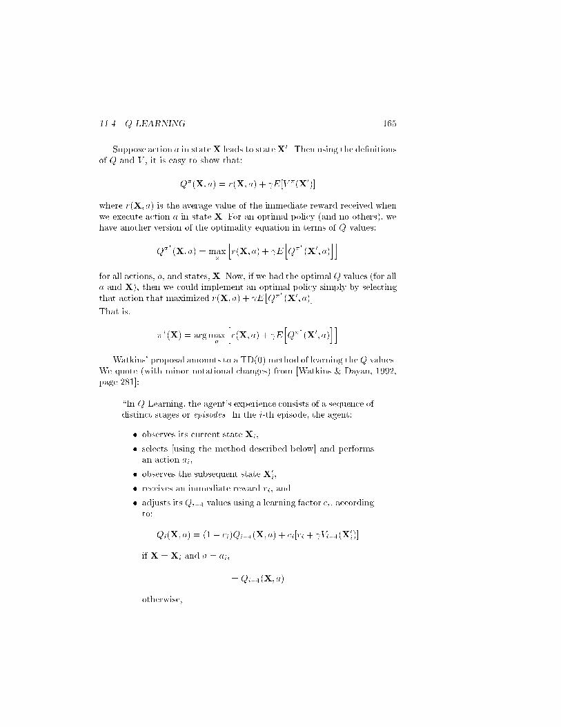
����� Q�LEARNING ��
Suppose action a in stateX leads to stateX�� Then using the de�nitionsof Q and V � it is easy to show that�
Q��X� a� r�X� a� # �E�V ��X���
where r�X� a� is the average value of the immediate reward received whenwe execute action a in state X� For an optimal policy �and no others�� wehave another version of the optimality equation in terms of Q values�
Q���X� a� maxa
hr�X� a� # �E
hQ���X�� a�
ii
for all actions� a� and states�X� Now� if we had the optimalQ values �for alla and X�� then we could implement an optimal policy simply by selectingthat action that maximized r�X� a� # �E
Q���X�� a�
��
That is�
��X� argmaxa
hr�X� a� # �E
hQ���X�� a�
ii
Watkins� proposal amounts to a TD� � method of learning theQ values�We quote �with minor notational changes� from �Watkins � Dayan� �����page �����
�In QLearning� the agent�s experience consists of a sequence ofdistinct stages or episodes� In the ith episode� the agent�
� observes its current state Xi�
� selects �using the method described below� and performsan action ai�
� observes the subsequent state X�i�
� receives an immediate reward ri� and
� adjusts its Qi�� values using a learning factor ci� accordingto�
Qi�X� a� ��� ci�Qi���X� a� # ci�ri # �Vi���X�i��
if X Xi and a ai�
Qi���X� a�
otherwise�

� CHAPTER ��� DELAYED�REINFORCEMENT LEARNING
where
Vi���X�� max
b�Qi���X
�� b��
is the best the agent thinks it can do from state X�� � � �The initial Q values� Q�X� a�� for all states and actionsare assumed given��
Using the current Q values� Qi�X� a�� the agent always selects that action that maximizes Qi�X� a�� Note that only the Q value correspondingto the state just exited and the action just taken is adjusted� And thatQ value is adjusted so that it is closer �by an amount determined by ci�to the sum of the immediate reward plus the discounted maximum �overall actions� of the Q values of the state just entered� If we imagine theQ values to be predictions of ultimate �in�nite horizon� total reward� thenthe learning procedure described above is exactly a TD� � method of learning how to predict these Q values� Q learning strengthens the usual TDmethods� however� because TD �applied to reinforcement problems usingvalue iteration� requires a onestep lookahead� using a model of the e�ectsof actions� whereas Q learning does not�
A convenient notation �proposed by �Schwartz� ������ for representingthe change in Q value is�
Q�X� a��� r # �V �X��
where Q�X� a� is the new Q value for input X and action a� r is the immediate reward when action a is taken in response to input X� V �X�� is themaximum �over all actions� of the Q value of the state next reached whenaction a is taken from state X� and � is the fraction of the way towardwhich the new Q value� Q�X� a�� is adjusted to equal r # �V �X���
Watkins and Dayan �Watkins � Dayan� ����� prove that� under certainconditions� the Q values computed by this learning procedure converge tooptimal ones �that is� to ones on which an optimal policy can be based��
We de�ne ni�X� a� as the index �episode number� of the ith time thataction a is tried in state X� Then� we have�
Theorem ���� �Watkins and Dayan� For Markov problems with statesfXg and actions fag� and given bounded rewards jrnj R� learning rates cn � �� and

����� DISCUSSION LIMITATIONS AND EXTENSIONSOFQ�LEARNING��
�Xi
cni�X�a� ���Xi
hcni�X�a�
i���
for all X and a� then
Qn�X� a�� Q�n�X� a� as n��� for all X and a� with probability �� where
Q�n�X� a� corresponds to the Q values of an optimal policy�
Again� we quote from �Watkins � Dayan� ����� page �����
�The most important condition implicit in the convergence theorem � � � is that the sequence of episodes that forms the basisof learning must include an in�nite number of episodes for eachstarting state and action� This may be considered a strong condition on the way states and actions are selected�however� under the stochastic conditions of the theorem� no method could beguaranteed to �nd an optimal policy under weaker conditions�Note� however� that the episodes need not form a continuoussequence�that is the X� of one episode need not be the X ofthe next episode��
The relationships amongQ learning� dynamic programming� and controlare very well described in �Barto� Bradtke� � Singh� ������ Q learning isbest thought of as a stochastic approximation method for calculating theQ values� Although the de�nition of the optimal Q values for any statedepends recursively on expected values of theQ values for subsequent states�and on the expected values of rewards�� no expected values are explicitlycomputed by the procedure� Instead� these values are approximated byiterative sampling using the actual stochastic mechanism that producessuccessor states�
���� Discussion� Limitations� and Exten
sions of QLearning
����� An Illustrative Example
The Qlearning procedure requires that we maintain a table of Q�X� a�values for all stateaction pairs� In the grid world that we described earlier�such a table would not be excessively large� We might start with randomentries in the table� a portion of such an intial table might be as follows�

�� CHAPTER ��� DELAYED�REINFORCEMENT LEARNING
X a Q�X� a� r�X� a�
����� w � ����� n � ����� e � ����� s ����� w � ������ n � ����� e � ����� s �
Suppose the robot is in cell ������ The maximum Q value occurs for a w�so the robot moves west to cell ������receiving no immediate reward� Themaximum Q value in cell ����� is �� and the learning mechanism attemptsto make the value of Q���� ��� w� closer to the discounted value of � plusthe immediate reward �which was in this case�� With a learning rateparameter c �� and � ��� the Q value of Q���� ��� w� is adjusted from� to ����� No other changes are made to the table at this episode� Thereader might try this learning procedure on the grid world with a simplecomputer program� Notice that an optimal policy might not be discoveredif some cells are not visited nor some actions not tried frequently enough�
The learning problem faced by the agent is to associate speci�c actionswith speci�c input patterns� Q learning gradually reinforces those actionsthat contribute to positive rewards by increasing the associated Q values�Typically� as in this example� rewards occur somewhat after the actionsthat lead to them�hence the phrase delayed�reinforcement learning� Onecan imagine that better and better approximations to the optimal Q valuesgradually propagate back from states producing rewards toward all of theother states that the agent frequently visits� With random Q values tobegin� the agent�s actions amount to a random walk through its space ofstates� Only when this random walk happens to stumble into rewardingstates does Q learning begin to produce Q values that are useful� and� eventhen� the Q values have to work their way outward from these rewardingstates� The general problem of associating rewards with stateaction pairsis called the temporal credit assignment problem�how should credit for areward be apportioned to the actions leading up to it� Q learning is� to date�the most successful technique for temporal credit assignment� although arelated method� called the bucket brigade algorithm� has been proposed by�Holland� �����
Learning problems similar to that faced by the agent in our grid world

����� DISCUSSION LIMITATIONS AND EXTENSIONSOFQ�LEARNING��
have been thoroughly studied by Sutton who has proposed an architecture�called DYNA� for solving them �Sutton� ��� �� DYNA combines reinforcement learning with planning� Sutton characterizes planning as learningin a simulated world that models the world that the agent inhabits� Theagent�s model of the world is obtained by Q learning in its actual world�and planning is accomplished by Q learning in its model of the world�
We should note that the learning problem faced by our gridworld robotcould be modi�ed to have several places in the grid that give positive rewards� This possibility presents an interesting way to generalize the classical notion of a �goal� in AI planning systems�even in those that do nolearning� Instead of representing a goal as a condition to be achieved� werepresent a �goal structure� as a set of rewards to be given for achieving various conditions� Then� the generalized �goal� becomes maximizingdiscounted future reward instead of simply achieving some particular condition� This generalization can be made to encompass socalled goals ofmaintenance and goals of avoidance� The example presented above included avoiding bumping into the gridworld boundary� A goal of maintenance� of a particular state� could be expressed in terms of a reward thatwas earned whenever the agent was in that state and performed an actionthat transitioned back to that state in one step�
����� Using Random Actions
When the next pattern presentation in a sequence of patterns is the onecaused by the agent�s own action in response to the last pattern� we havewhat is called an on�line learning method� In Watkins and Dayan�s terminology� in online learning the episodes form a continous sequence� Asalready mentioned� the convergence theorem forQ learning does not requireonline learning� indeed� special precautions must be taken to ensure thatonline learning meets the conditions of the theorem� If online learningdiscovers some good paths to rewards� the agent may �xate on these andnever discover a policy that leads to a possibly greater longterm reward�In reinforcement learning phraseology� this problem is referred to as theproblem of exploitation �of already learned behavior� versus exploration �ofpossibly better behavior��
One way to force exploration is to perform occasional random actions�instead of that single action prescribed by the current Q values�� Forexample� in the gridworld problem� one could imagine selecting an actionrandomly according to a probability distribution over the actions �n� e� s�and w�� This distribution� in turn� could depend on the Q values� Forexample� we might �rst �nd that action prescribed by the Q values and

�� CHAPTER ��� DELAYED�REINFORCEMENT LEARNING
then choose that action with probability ���� choose the two orthogonalactions with probability ��� each� and choose the opposite action withprobability ���� This policy might be modi�ed by �simulated annealing�which would gradually increase the probability of the action prescribed bythe Q values more and more as time goes on� This strategy would favorexploration at the beginning of learning and exploitation later�
Other methods� also� have been proposed for dealing with exploration�including making unvisited states intrinsically rewarding and using an �interval estimate�� which is related to the uncertainty in the estimate of astate�s value �Kaelbling� ������
����� Generalizing Over Inputs
For large problems it would be impractical to maintain a table like that usedin our gridworld example� Various researchers have suggested mechanismsfor computing Q values� given pattern inputs and actions� One methodthat suggests itself is to use a neural network� For example� consider thesimple linear machine shown in Fig� �����
X. . .
. . .
Σ
Σ
Σ
trainable weights
Σ
Wi
R dot product units
Q(ai, X) = X . Wi
Q(a1, X)
Q(a2, X)
Q(aR, X)
Figure ����� A Net that Computes Q Values

����� DISCUSSION LIMITATIONS AND EXTENSIONSOFQ�LEARNING���
Such a neural net could be used by an agent that has R actions to selectfrom� The Q values �as a function of the input pattern X and the actionai� are computed as dot products of weight vectors �one for each action�and the input vector� Weight adjustments are made according to a TD� �procedure to bring the Q value for the action last selected closer to the sumof the immediate reward �if any� and the �discounted� maximum Q valuefor the next input pattern�
If the optimum Q values for the problem �whatever they might be�are more complex than those that can be computed by a linear machine� alayered neural network might be used� Sigmoid units in the �nal layer wouldcompute Q values in the range to �� The TD� � method for updating Qvalues would then have to be combined with a multilayer weightchangingrule� such as backpropagation�
Networks of this sort are able to aggregate di�erent input vectors intoregions for which the same action should be performed� This kind of aggregation is an example of what has been called structural credit assignment�Combining TD��� and backpropagation is a method for dealing with boththe temporal and the structural credit assignment problems�
Interesting examples of delayedreinforcement training of simulated andactual robots requiring structural credit assignment have been reported by�Lin� ����� Mahadevan � Connell� ������
����� Partially Observable States
So far� we have identi�ed the input vector� X� with the actual state of theenvironment� When the input vector results from an agent�s perceptualapparatus �as we assume it does�� there is no reason to suppose that ituniquely identi�es the environmental state� Because of inevitable perceptual limitations� several di�erent environmental states might give rise tothe same input vector� This phenomenon has been referred to as percep�tual aliasing� With perceptual aliasing� we can no longer guarantee thatQ learning will result in even useful action policies� let alone optimal ones�Several researchers have attempted to deal with this problem using a variety of methods including attempting to model �hidden� states by usinginternal memory �Lin� ������ That is� if some aspect of the environmentcannot be sensed currently� perhaps it was sensed once and can be remembered by the agent� When such is the case� we no longer have a Markovproblem� that is� the next X vector� given any action� may depend on asequence of previous ones rather than just the immediately preceding one�It might be possible to reinstate a Markov framework �over the X�s� if X

��� CHAPTER ��� DELAYED�REINFORCEMENT LEARNING
includes not only current sensory precepts but information from the agent�smemory�
���� Scaling Problems
Several di�culties have so far prohibited wide application of reinforcementlearning to large problems� �The TDgammon program� mentioned in thelast chapter� is probably unique in terms of success on a highdimensionalproblem�� We have already touched on some di�culties� these and othersare summarized below with references to attempts to overcome them�
a� Exploration versus exploitation�
� use random actions
� favor states not visited recently
� separate the learning phase from the use phase
� employ a teacher to guide exploration
b� Slow time to convergence
� combine learning with prior knowledge� use estimates ofQ values�rather than random values� initially
� use a hierarchy of actions� learn primitive actions �rst and freezethe useful sequences into macros and then learn how to use themacros
� employ a teacher� use graded �lessons��starting near the rewards and then backing away� and use examples of good behavior�Lin� �����
� use more e�cient computations� e�g� do several updates perepisode �Moore � Atkeson� �����
c� Large state spaces
� use handcoded features
� use neural networks
� use nearestneighbor methods �Moore� ��� �
d� Temporal discounting problems� Using small � can make the learnertoo greedy for present rewards and indi�erent to the future� but usinglarge � slows down learning�

����� BIBLIOGRAPHICAL AND HISTORICAL REMARKS ���
� use a learning method based on average rewards �Schwartz� �����
e� No �transfer� of learning � What is learned depends on the rewardstructure� if the rewards change� learning has to start over�
� Separate the learning into two parts� learn an �action model�which predicts how actions change states �and is constant overall problems�� and then learn the �values� of states by reinforcement learning for each di�erent set of rewards� Sometimes thereinforcement learning part can be replaced by a �planner� thatuses the action model to produce plans to achieve goals�
Also see other articles in the special issue on reinforcement learning�Machine Learning� �� May� �����
��� Bibliographical and Historical RemarksTo be added�

��� CHAPTER ��� DELAYED�REINFORCEMENT LEARNING

Chapter ��
Explanation�Based
Learning
���� Deductive Learning
In the learning methods studied so far� typically the training set does notexhaust the version space� Using logical terminology� we could say thatthe classi�er�s output does not logically follow from the training set� Inthis sense� these methods are inductive� In logic� a deductive system is onewhose conclusions logically follow from a set of input facts� if the system issound��
To contrast inductive with deductive systems in a logical setting� suppose we have a set of facts �the training set� that includes the followingformulas�
fRound�Obj��� Round�Obj��� Round�Obj��� Round�Obj���
Ball�Obj��� Ball�Obj��� Ball�Obj��� Ball�Obj��g
A learning system that forms the conclusion ��x��Ball�x� � Round�x��is inductive� This conclusion may be useful �if there are no facts of theform Ball�����Round����� but it does not logically follow from the facts�On the other hand� if we had the facts Green�Obj�� and Green�Obj�� �
�Logical reasoning systems that are not sound� for example those using non monotonicreasoning� themselves might produce inductive conclusions that do not logically followfrom the input facts�
���

�� CHAPTER ��� EXPLANATION�BASED LEARNING
Round�Obj��� then we could logically conclude Round�Obj��� Making thisconclusion and saving it is an instance of deductive learning�a topic westudy in this chapter�
Suppose that some logical proposition� � logically follows from someset of facts� �� Under what circumstances might we say that the processof deducing from � results in our learning � In a sense� we implicitlyknew all along� since it was inherent in knowing �� Yet� might not beobvious given �� and the deduction process to establish might have beenarduous� Rather than have to deduce again� we might want to save it�perhaps along with its deduction� in case it is needed later� Shouldn�t thatprocess count as learning� Dietterich �Dietterich� ��� � has called this typeof learning speed�up learning�
Strictly speaking� speedup learning does not result in a system beingable to make decisions that� in principle� could not have been made beforethe learning took place� Speedup learning simply makes it possible to makethose decisions more e�ciently� But� in practice� this type of learning mightmake possible certain decisions that might otherwise have been infeasible�
To take an extreme case� a chess player can be said to learn chess eventhough optimal play is inherent in the rules of chess� On the surface� thereseems to be no real di�erence between the experiencebased hypothesesthat a chess player makes about what constitutes good play and the kindof learning we have been studying so far�
As another example� suppose we are given some theorems about geometry and are asked to prove that the sum of the angles of a right triangleis �� degrees� Let us further suppose that the proof we constructed didnot depend on the given triangle being a right triangle� in that case wecan learn a more general fact� The learning technique that we are going tostudy next is related to this example� It is called explanation�based learning�EBL�� EBL can be thought of as a process in which implicit knowledge isconverted into explicit knowledge�
In EBL� we specialize parts of a domain theory to explain a particularexample� then we generalize the explanation to produce another element ofthe domain theory that will be useful on similar examples� This process isillustrated in Fig� �����
���� Domain Theories
Two types of information were present in the inductive methods we havestudied� the information inherent in the training samples and the information about the domain that is implied by the �bias� �for example� the

����� DOMAIN THEORIES ���
DomainTheory
Example(X is P)
Prove: X is P
specialize
Explanation(Proof)
generalize
A New Domain Rule:Things "like" X are P
Y is like X
Complex ProofProcess
Trivial Proof
Y is P
Figure ����� The EBL Process
hypothesis set from which we choose functions�� The learning methods aresuccessful only if the hypothesis set is appropriate for the problem� Typically� the smaller the hypothesis set �that is� the more a priori informationwe have about the function being sought�� the less dependent we are oninformation being supplied by a training set �that is� fewer samples�� Apriori information about a problem can be expressed in several ways� Themethods we have studied so far restrict the hypotheses in a rather directway� A less direct method involves making assertions in a logical languageabout the property we are trying to learn� A set of such assertions is usuallycalled a �domain theory��
Suppose� for example� that we wanted to classify people according towhether or not they were good credit risks� We might represent a person

��� CHAPTER ��� EXPLANATION�BASED LEARNING
by a set of properties �income� marital status� type of employment� etc���assemble such data about people who are known to be good and bad creditrisks and train a classi�er to make decisions� Or� we might go to a loano�cer of a bank� ask him or her what sorts of things s�he looks for inmaking a decision about a loan� encode this knowledge into a set of rulesfor an expert system� and then use the expert system to make decisions�The knowledge used by the loan o�cer might have originated as a setof �policies� �the domain theory�� but perhaps the application of thesepolicies were specialized and made more e�cient through experience withthe special cases of loans made in his or her district�
���� An Example
To make our discussion more concrete� let�s consider the following fancifulexample� We want to �nd a way to classify robots as �robust� or not� Theattributes that we use to represent a robot might include some that arerelevant to this decision and some that are not�
Suppose we have a domain theory of logical sentences that taken together� help to de�ne whether or not a robot can be classi�ed as robust��The same domain theory may be useful for several other purposes also�but among other things� it describes the concept �robust���
In this example� let�s suppose that our domain theory includes the sentences�
Fixes�u� u� � Robust�u�
�An individual that can �x itself is robust��
Sees�x� y� �Habile�x� � Fixes�x� y�
�A habile individual that can see another entity can �x that entity��
Robot�w� � Sees�w�w�
�All robots can see themselves��
R�D��x� � Habile�x�
�R�D�class individuals are habile��
C�PO�x� � Habile�x�

����� AN EXAMPLE ���
�C�POclass individuals are habile��
� � �
�By convention� variables are assumed to be universally quanti�ed�� Wecould use theoremproving methods operating on this domain theory toconclude whether certain robots are robust� These methods might be computationally quite expensive because extensive search may have to be performed to derive a conclusion� But after having found a proof for someparticular robot� we might be able to derive some new sentence whose useallows a much faster conclusion�
We next show how such a new rule might be derived in this example�Suppose we are given a number of facts about Num�� such as�
Robot�Num��
R�D��Num��
Age�Num�� ��
Manufacturer�Num�� GR�
� � �
We are also told that Robust�Num�� is true� but we nevertheless attemptto �nd a proof of that assertion using these facts about Num� and thedomain theory� The facts about Num� correspond to the features that wemight use to represent Num�� In this example� not all of them are relevantto a decision about Robust�Num��� The relevant ones are those used orneeded in proving Robust�Num�� using the domain theory� The proof treein Fig� ���� is one that a typical theoremproving system might produce�
In the language of EBL� this proof is an explanation for the factRobust�Num��� We see from this explanation that the only facts aboutNum� that were used were Robot�Num�� and R�D��Num��� In fact� wecould construct the following rule from this explanation�
Robot�Num���R�D��Num�� � Robust�Num��
The explanation has allowed us to prune some attributes about Num� thatare irrelevant �at least for deciding Robust�Num���� This type of pruning isthe �rst sense in which an explanation is used to generalize the classi�cationproblem� ��DeJong � Mooney� ���� call this aspect of explanationbased

�� CHAPTER ��� EXPLANATION�BASED LEARNING
Fixes(u, u) => Robust(u)
Robust(Num5)
Fixes(Num5, Num5)
Sees(Num5,Num5) Habile(Num5)
Sees(x,y) & Habile(x) => Fixes(x,y)
Robot(w) => Sees(w,w)
Robot(Num5)
R2D2(x) => Habile(x)
R2D2(Num5)
Figure ����� A Proof Tree
learning feature elimination�� But the rule we extracted from the explanation applies only to Num�� There might be little value in learning thatrule since it is so speci�c� Can it be generalized so that it can be appliedto other individuals as well�
Examination of the proof shows that the same proof structure� usingthe same sentences from the domain theory� could be used independentlyof whether we are talking about Num� or some other individual� We cangeneralize the proof by a process that replaces constants in the tip nodesof the proof tree with variables and works upward�using uni�cation toconstrain the values of variables as needed to obtain a proof�
In this example� we replaceRobot�Num�� byRobot�r� andR�D��Num��by R�D��s� and redo the proof�using the explanation proof as a template�Note that we use di�erent values for the two di�erent occurrences of Num�at the tip nodes� Doing so sometimes results in more general� but nevertheless valid rules� We now apply the rules used in the proof in the forwarddirection� keeping track of the substitutions imposed by the most general

����� AN EXAMPLE ���
uni�ers used in the proof� �Note that we always substitute terms that arealready in the tree for variables in rules�� This process results in the generalized proof tree shown in Fig� ����� Note that the occurrence of Sees�r� r�as a node in the tree forces the uni�cation of x with y in the domain rule�Sees�x� y� � Habile�y� � Fixes�x� y�� The substitutions are then appliedto the variables in the tip nodes and the root node to yield the general rule�Robot�r��R�D��r� � Robust�r��
Robust(r)
Fixes(r, r)
Sees(r,r) Habile(s)
Robot(r) R2D2(s)
{r/w}{s/x}
{r/x, r/y, r/s}
{r/u}
Robot(w) => Sees(w,w)
R2D2(x) => Habile(x)
Sees(x,y) & Habile(x) => Fixes(x,y)
Fixes(u, u) => Robust(u)
becomes R2D2(r) afterapplying {r/s}
Figure ����� A Generalized Proof Tree
This rule is the end result of EBL for this example� The processby which Num� in this example was generalized to a variable is what�DeJong � Mooney� ���� call identity elimination �the precise identity ofNum� turned out to be irrelevant�� �The generalization process describedin this example is based on that of �DeJong � Mooney� ���� and differs from that of �Mitchell� et al�� ����� It is also similar to that used

��� CHAPTER ��� EXPLANATION�BASED LEARNING
in �Fikes� et al�� ������� Clearly� under certain assumptions� this generalrule is more easily used to conclude Robust about an individual than theoriginal proof process was�
It is important to note that we could have derived the general rule fromthe domain theory without using the example� �In the literature� doing so iscalled static analysis �Etzioni� ������� In fact� the example told us nothingnew other than what it told us about Num�� The sole role of the examplein this instance of EBL was to provide a template for a proof to help guidethe generalization process� Basing the generalization process on exampleshelps to insure that we learn rules matched to the distribution of problemsthat occur�
There are a number of quali�cations and elaborations about EBL thatneed to be mentioned�
���� Evaluable Predicates
The domain theory includes a number of predicates other than the oneoccuring in the formula we are trying to prove and other than those thatmight customarily be used to describe an individual� One might note� forexample� that if we usedHabile�Num�� to describe Num�� the proof wouldhave been shorter� Why didn�t we� The situation is analogous to that ofusing a data base augmented by logical rules� In the latter application� theformulas in the actual data base are �extensional�� and those in the logicalrules are �intensional�� This usage re�ects the fact that the predicates inthe data base part are de�ned by their extension�we explicitly list all thetuples sastisfying a relation� The logical rules serve to connect the data basepredicates with higher level abstractions that are described �if not de�ned�by the rules� We typically cannot look up the truth values of formulascontaining these intensional predicates� they have to be derived using therules and the database�
The EBL process assumes something similar� The domain theory is useful for connecting formulas that we might want to prove with those whosetruth values can be �looked up� or otherwise evaluated� In the EBL literature� such formulas satisfy what is called the operationality criterion�Perhaps another analogy might be to neural networks� The evaluable predicates correspond to the components of the input pattern vector� the predicates in the domain theory correspond to the hidden units� Finding thenew rule corresponds to �nding a simpler expression for the formula to beproved in terms only of the evaluable predicates�

����� MORE GENERAL PROOFS ���
���� More General Proofs
Examining the domain theory for our example reveals that an alternativerule might have been� Robot�u� � C�PO�u� � Robust�u�� Such a rulemight have resulted if we were given fC�PO�Num�� Robot�Num�� � � �gand proved Robust�Num�� After considering these two examples �Num�and Num�� the question arises� do we want to generalize the two rules tosomething like� Robot�u�� �C�PO�u��R�D��u��� Robust�u�� Doing so isan example of what �DeJong � Mooney� ���� call structural generalization�via disjunctive augmentation ��
Adding disjunctions for every alternative proof can soon become cumbersome and destroy any e�ciency advantage of EBL� In our example�the e�ciency might be retrieved if there were another evaluable predicate�say� Bionic�u� such that the domain theory also contained R�D��x� �Bionic�x� and C�PO�x� � Bionic�x�� After seeing a number of similar examples� we might be willing to induce the formula Bionic�u� ��C�PO�u� � R�D��u�� in which case the rule with the disjunction couldbe replaced with Robot�u��Bionic�u� � Robust�u��
��� Utility of EBL
It is well known in theorem proving that the complexity of �nding a proofdepends both on the number of formulas in the domain theory and on thedepth of the shortest proof� Adding a new rule decreases the depth of theshortest proof but it also increases the number of formulas in the domaintheory� In realistic applications� the added rules will be relevant for sometasks and not for others� Thus� it is unclear whether the overall utility ofthe new rules will turn out to be positive� EBL methods have been appliedin several settings� usually with positive utility� �See �Minton� ��� � for ananalysis��
���� Applications
There have been several applications of EBL methods� We mention twohere� namely the formation of macrooperators in automatic plan generationand learning how to control search�

��� CHAPTER ��� EXPLANATION�BASED LEARNING
������ Macro�Operators in Planning
In automatic planning systems� e�ciency can sometimes be enhanced bychaining together a sequence of operators into macro�operators� We showan example of a process for creating macrooperators based on techniquesexplored by �Fikes� et al�� ������
Referring to Fig� ����� consider the problem of �nding a plan for arobot in room R� to fetch a box� B�� by going to an adjacent room� R��and pushing it back to R�� The goal for the robot is INROOM�B�� R���and the facts that are true in the initial state are listed in the �gure�
R1 R2
R3
D1
D2
B1
Initial State:
INROOM(ROBOT, R1)INROOM(B1,R2)CONNECTS(D1,R1,R2)CONNECTS(D1,R2,R1)
. . .
Figure ����� Initial State of a Robot Problem
We will construct the plan from a set of STRIPS operators that include�
GOTHRU�d� r�� r��
Preconditions� INROOM�ROBOT� r��� CONNECTS�d� r�� r��
Delete list� INROOM�ROBOT� r��
Add list� INROOM�ROBOT� r��

����� APPLICATIONS ���
PUSHTHRU�b� d� r�� r��
Preconditions� INROOM�ROBOT� r��� CONNECTS�d� r�� r��� INROOM�b� r��
Delete list� INROOM�ROBOT� r��� INROOM�b� r��
Add list� INROOM�ROBOT� r��� INROOM�b� r��
A backwardreasoning STRIPS system might produce the plan shownin Fig� ����� We show there the main goal and the subgoals along a solutionpath� �The conditions in each subgoal that are true in the initial state areshown underlined�� The preconditions for this plan� true in the initial state�are�
INROOM�ROBOT�R��
CONNECTS�D�� R�� R��
CONNECTS�D�� R�� R��
INROOM�B�� R��
Saving this speci�c plan� valid only for the speci�c constants it mentions�would not be as useful as would be saving a more general one� We �rstgeneralize these preconditions by substituting variables for constants� Wethen follow the structure of the speci�c plan to produce the generalizedplan shown in Fig� ��� that achieves INROOM�b�� r��� Note that thegeneralized plan does not require pushing the box back to the place wherethe robot started� The preconditions for the generalized plan are�
INROOM�ROBOT� r��
CONNECTS�d�� r�� r��
CONNECTS�d�� r�� r��
INROOM�b� r��
Another related technique that chains together sequences of operators to form more general ones is the chunking mechanism in Soar�Laird� et al�� �����

�� CHAPTER ��� EXPLANATION�BASED LEARNING
INROOM(B1,R1)
PUSHTHRU(B1,d,r1,R1)
INROOM(ROBOT, r1),CONNECTS(d, r1, R1),INROOM(B1, r1)
INROOM(ROBOT, R2),CONNECTS(D1, R2, R1),INROOM(B1, R2){R2/r1,
D1/d}
GOTHRU(d2, r3, R2)
INROOM(ROBOT, r3),CONNECTS(d2, r3, R2),CONNECTS(D1, R2, R1),INROOM(B1, R2)
{R1/r3, D1/d2}
INROOM(ROBOT, R1),CONNECTS(D1, R1, R2),CONNECTS(D1, R2, R1),INROOM(B1, R2)
R1 R2
R3
D1
D2
GOTHRU(D1,R1,R2)PUSHTHRU(B1,D1,R2,R1)
B1
PLAN:
Figure ����� A Plan for the Robot Problem
������ Learning Search Control Knowledge
Besides their use in creating macrooperators� EBL methods can be used toimprove the e�ciency of planning in another way also� In his system calledPRODIGY� Minton proposed using EBL to learn e�ective ways to controlsearch �Minton� ������ PRODIGY is a STRIPSlike system that solvesplanning problems in the blocksworld� in a simple mobile robot world� andin jobshop scheduling� PRODIGY has a domain theory involving both thedomain of the problem and a simple �meta� theory about planning� Itsmeta theory includes statements about whether a control choice about asubgoal to work on� an operator to apply� etc� either succeeds or fails� Afterproducing a plan� it analyzes its successful and its unsuccessful choices andattempts to explain them in terms of its domain theory� Using an EBLlikeprocess� it is able to produce useful control rules such as�

���� BIBLIOGRAPHICAL AND HISTORICAL REMARKS ���
INROOM(b1,r4)
PUSHTHRU(b1,d2,r2,r4)
INROOM(ROBOT, r2),CONNECTS(d1, r1, r2),CONNECTS(d2, r2, r4),INROOM(b1, r4)
GOTHRU(d1, r1, r2)
INROOM(ROBOT, r1),CONNECTS(d1, r1, r2),CONNECTS(d2, r2, r4),INROOM(b1, r4)
Figure ���� A Generalized Plan
IF �AND �CURRENT� NODE node�
�CANDIDATE� GOAL node �ON x y��
�CANDIDATE � GOAL node �ON y z���
THEN �PREFER GOAL �ON y z� TO �ON x y��
PRODIGY keeps statistics on how often these learned rules are used� theirsavings �in time to �nd plans�� and their cost of application� It savesonly the rules whose utility� thus measured� is judged to be high� Minton�Minton� ��� � has shown that there is an overall advantage of using theserules �as against not having any rules and as against handcoded searchcontrol rules��
��� Bibliographical and Historical RemarksTo be added�

��� CHAPTER ��� EXPLANATION�BASED LEARNING

Bibliography
�Acorn � Walden� ����� Acorn� T�� and Walden� S�� �SMART� SupportManagement Automated Reasoning Technology for COMPAQ Customer Service�� Proc� Fourth Annual Conf� on Innovative Applica�tions of Arti�cial Intelligence� Menlo Park� CA� AAAI Press� �����
�Aha� ����� Aha� D�� Kibler� D�� and Albert� M�� �InstanceBased LearningAlgorithms�� Machine Learning� � ��� �����
�Anderson � Bower� ����� Anderson� J� R�� and Bower� G� H�� Human As�sociative Memory� Hillsdale� NJ� Erlbaum� �����
�Anderson� ����� Anderson� T� W�� An Introduction to Multivariate Statis�tical Analysis� New York� John Wiley� �����
�Barto� Bradtke� � Singh� ����� Barto� A�� Bradtke� S�� and Singh� S���Learning to Act Using RealTime Dynamic Programming�� to appear in Arti�cial Intelligence� �����
�Baum � Haussler� ����� Baum� E� and Haussler� D�� �What Size NetGives Valid Generalization�� Neural Computation� �� pp� ���� ������
�Baum� ����� Baum� E�� �When Are kNearest Neighbor and Backpropagation Accurate for FeasibleSized Sets of Examples�� in Hanson� S�� Drastal� G�� and Rivest� R�� �eds��� Computational LearningTheory and Natural Learning Systems� Volume �� Constraints andProspects� pp� ������� Cambridge� MA� MIT Press� �����
�Bellman� ����� Bellman� R� E�� Dynamic Programming� Princeton�Princeton University Press� �����
�Blumer� et al�� ����� Blumer� A�� et al�� �Occam�s Razor�� Info� Process�Lett�� vol �� pp� ���� � �����
���

�� BIBLIOGRAPHY
�Blumer� et al�� ��� � Blumer� A�� et al�� �Learnability and the VapnikChervonenkis Dimension�� JACM� ��� �
�Bollinger � Du�e� ����� Bollinger� J�� and Du�e� N�� Computer Controlof Machines and Processes� Reading� MA� AddisonWesley� �����
�Brain� et al�� ���� Brain� A� E�� et al�� �Graphical Data Processing Research Study and Experimental Investigation�� Report No� � �pp����� and No� � �pp� �� �� Contract DA � �� SC������ SRI International� Menlo Park� CA� June ��� and September ����
�Breiman� et al�� ����� Breiman� L�� Friedman� J�� Olshen� R�� and Stone�C�� Classi�cation and Regression Trees� Monterey� CA� Wadsworth������
�Brent� ��� � Brent� R� P�� �Fast Training Algorithms for MultiLayer Neural Nets�� Numerical Analysis Project Manuscript NA� �� Computer Science Department� StanfordUniversity� Stanford� CA ��� ��March ��� �
�Bryson � Ho ���� Bryson� A�� and Ho� Y�C�� Applied Optimal Control�New York� Blaisdell�
�Buchanan � Wilkins� ����� Buchanan� B� and Wilkins� D�� �eds��� Read�ings in Knowledge Acquisition and Learning� San Francisco� MorganKaufmann� �����
�Carbonell� ����� Carbonell� J�� �Learning by Analogy�� in Machine Learn�ing� An Arti�cial Intelligence Approach� Michalski� R�� Carbonell�J�� and Mitchell� T�� �eds��� San Francisco� Morgan Kaufmann� �����
�Cheeseman� et al�� ����� Cheeseman� P�� et al�� �AutoClass� A BayesianClassi�cation System�� Proc� Fifth Intl� Workshop on MachineLearning� Morgan Kaufmann� San Mateo� CA� ����� Reprinted inShavlik� J� and Dietterich� T�� Readings in Machine Learning� Morgan Kaufmann� San Francisco� pp� ��� � ��� �
�Cover � Hart� ���� Cover� T�� and Hart� P�� �Nearest Neighbor Pattern Classi�cation�� IEEE Trans� on Information Theory� ��� ���������
�Cover� ���� Cover� T�� �Geometrical and Statistical Properties of Systemsof Linear Inequalities with Applications in Pattern Recognition��IEEE Trans� Elec� Comp�� EC��� ������ June� ����

BIBLIOGRAPHY ���
�Dasarathy� ����� Dasarathy� B� V�� Nearest Neighbor Pattern Classi�ca�tion Techniques� IEEE Computer Society Press� �����
�Dayan � Sejnowski� ����� Dayan� P�� and Sejnowski� T�� �TD��� Converges with Probability ���Machine Learning� ��� pp� ���� �� �����
�Dayan� ����� Dayan� P�� �The Convergence of TD��� for General ��� Ma�chine Learning� �� ������ �����
�DeJong � Mooney� ���� DeJong� G�� and Mooney� R�� �ExplanationBased Learning� An Alternative View�� Machine Learning� �������� ���� Reprinted in Shavlik� J� and Dietterich� T�� Readingsin Machine Learning� San Francisco� Morgan Kaufmann� ��� � pp������
�Dietterich � Bakiri� ����� Dietterich� T� G�� and Bakiri� G�� �ErrorCorrecting Output Codes� A General Method for Improving Multiclass Inductive Learning Programs�� Proc� Ninth Nat� Conf� onA�I�� pp� ������� AAAI��� MIT Press� �����
�Dietterich� et al�� ��� � Dietterich� T�� Hild� H�� and Bakiri� G�� �A Comparative Study of ID� and Backpropagation for English TexttoSpeechMapping�� Proc� Seventh Intl� Conf� Mach� Learning� Porter�B� and Mooney� R� �eds��� pp� ����� San Francisco� Morgan Kaufmann� ��� �
�Dietterich� ��� � Dietterich� T�� �Machine Learning��Annu� Rev� Comput�Sci�� ������ � Palo Alto� Annual Reviews Inc�� ��� �
�Duda � Fossum� ��� Duda� R� O�� and Fossum� H�� �Pattern Classi�cation by Iteratively Determined Linear and Piecewise Linear Discriminant Functions�� IEEE Trans� on Elect� Computers� vol� EC��� pp��� ���� April� ���
�Duda � Hart� ����� Duda� R� O�� and Hart� P�E�� Pattern Classi�cationand Scene Analysis� New York� Wiley� �����
�Duda� ��� Duda� R� O�� �Training a Linear Machine on MislabeledPatterns�� SRI Tech� Report prepared for ONR under Contract����� �� SRI International� Menlo Park� CA� April ���
�Efron� ����� Efron� B�� The Jackknife� the Bootstrap and Other Resam�pling Plans� Philadelphia� SIAM� �����

��� BIBLIOGRAPHY
�Ehrenfeucht� et al�� ����� Ehrenfeucht� A�� et al�� �A General LowerBound on the Number of Examples Needed for Learning�� in Proc����� Workshop on Computational Learning Theory� pp� �� �� �San Francisco� Morgan Kaufmann� �����
�Etzioni� ����� Etzioni� O�� �STATIC� A ProblemSpace Compiler forPRODIGY�� Proc� of Ninth National Conf� on Arti�cial Intelli�gence� pp� ����� � Menlo Park� AAAI Press� �����
�Etzioni� ����� Etzioni� O�� �A Structural Theory of ExplanationBasedLearning�� Arti�cial Intelligence� ��� pp� ������ March� �����
�Evans � Fisher� ����� Evans� B�� and Fisher� D�� Process Delay AnalysesUsing Decision�Tree Induction� Tech� Report CS�� � Departmentof Computer Science� Vanderbilt University� TN� �����
�Fahlman � Lebiere� ��� � Fahlman� S�� and Lebiere� C�� �The CascadeCorrelation Learning Architecture�� in Touretzky� D�� �ed��� Ad�vances in Neural Information Processing Systems� � pp� �������San Francisco� Morgan Kaufmann� ��� �
�Fayyad� et al�� ����� Fayyad� U� M�� Weir� N�� and Djorgovski� S�� �SKICAT� A Machine Learning System for Automated Cataloging ofLarge Scale Sky Surveys�� in Proc� Tenth Intl� Conf� on MachineLearning� pp� ������� San Francisco� Morgan Kaufmann� ������For a longer version of this paper see� Fayyad� U� Djorgovski� G��and Weir� N�� �Automating the Analysis and Cataloging of Sky Surveys�� in Fayyad� U�� et al��eds��� Advances in Knowledge Discoveryand Data Mining� Chapter ��� pp� ������ Cambridge� The MITPress� March� �����
�Feigenbaum� ���� Feigenbaum� E� A�� �The Simulation of Verbal Learning Behavior�� Proceedings of the Western Joint Computer Confer�ence� ���������� ����
�Fikes� et al�� ����� Fikes� R�� Hart� P�� and Nilsson� N�� �Learning andExecuting Generalized Robot Plans�� Arti�cial Intelligence� pp ������� ����� Reprinted in Shavlik� J� and Dietterich� T�� Readings inMachine Learning� San Francisco� Morgan Kaufmann� ��� � pp �����
�Fisher� ����� Fisher� D�� �Knowledge Acquisition via Incremental Conceptual Clustering�� Machine Learning� ��������� ����� Reprinted inShavlik� J� and Dietterich� T�� Readings in Machine Learning� SanFrancisco� Morgan Kaufmann� ��� � pp� ��)����

BIBLIOGRAPHY ���
�Friedman� et al�� ����� Friedman� J� H�� Bentley� J� L�� and Finkel� R� A���An Algorithm for Finding Best Matches in Logarithmic ExpectedTime�� ACM Trans� on Math� Software� ������ ���� September�����
�Fu� ����� Fu� L�� Neural Networks in Arti�cial Intelligence� New York�McGrawHill� �����
�Gallant� ���� Gallant� S� I�� �Optimal Linear Discriminants�� in EighthInternational Conf� on Pattern Recognition� pp� ������� New York�IEEE� ����
�Genesereth � Nilsson� ����� Genesereth� M�� and Nilsson� N�� LogicalFoundations of Arti�cial Intelligence� San Francisco� Morgan Kaufmann� �����
�Gluck � Rumelhart� ����� Gluck� M� and Rumelhart� D�� Neuroscienceand Connectionist Theory� The Developments in Connectionist Theory� Hillsdale� NJ� Erlbaum Associates� �����
�Hammerstrom� ����� Hammerstrom� D�� �Neural Networks at Work��IEEE Spectrum� pp� ���� June �����
�Haussler� ����� Haussler� D�� �Quantifying Inductive Bias� AI LearningAlgorithms and Valiant�s Learning Framework�� Arti�cial Intelli�gence� ��������� ����� Reprinted in Shavlik� J� and Dietterich� T��Readings in Machine Learning� San Francisco� Morgan Kaufmann���� � pp� �� ��
�Haussler� ��� � Haussler� D�� �Probably Approximately Correct Learning�� Proc� Eighth Nat� Conf� on AI� pp� �� ��� �� Cambridge�MA� MIT Press� ��� �
�Hebb� ����� Hebb� D� O�� The Organization of Behaviour� New York� JohnWiley� �����
�Hertz� Krogh� � Palmer� ����� Hertz� J�� Krogh� A� and Palmer� R�� In�troduction to the Theory of Neural Computation� Lecture Notes� vol��� Santa Fe Inst� Studies in the Sciences of Complexity� New York�AddisonWesley� �����
�Hirsh� ����� Hirsh� H�� �Generalizing Version Spaces�� Machine Learning���� ���� �����

��� BIBLIOGRAPHY
�Holland� ����� Holland� J�� Adaptation in Natural and Arti�cial Systems�Ann Arbor� The University of Michigan Press� ����� �Second editionprinted in ���� by MIT Press� Cambridge� MA��
�Holland� ���� Holland� J� H�� �Escaping Brittleness� The Possibilitiesof GeneralPurpose Learning Algorithms Applied to Parallel RuleBased Systems�� In Michalski� R�� Carbonell� J�� and Mitchell� T��eds�� � Machine Learning� An Arti�cial Intelligence Approach� Vol�ume � chapter � � San Francisco� Morgan Kaufmann� ����
�Hunt� Marin� � Stone� ��� Hunt� E�� Marin� J�� and Stone� P�� Experi�ments in Induction� New York� Academic Press� ���
�Jabbour� K�� et al�� ����� Jabbour� K�� et al�� �ALFA� Automated LoadForecasting Assistant�� Proc� of the IEEE Pwer Engineering SocietySummer Meeting� San Francisco� CA� �����
�John� ����� John� G�� �Robust Linear Discriminant Trees�� Proc� of theConf� on Arti�cial Intelligence and Statistics� Ft� Lauderdale� FL�January� �����
�Kaelbling� ����� Kaelbling� L� P�� Learning in Embedded Systems� Cambridge� MA� MIT Press� �����
�Kohavi� ����� Kohavi� R�� �BottomUp Induction of Oblivious ReadOnceDecision Graphs�� Proc� of European Conference on Machine Learn�ing �ECML����� �����
�Kolodner� ����� Kolodner� J�� Case�Based Reasoning� San Francisco� Morgan Kaufmann� �����
�Koza� ����� Koza� J�� Genetic Programming� On the Programming ofComputers by Means of Natural Selection� Cambridge� MA� MITPress� �����
�Koza� ����� Koza� J�� Genetic Programming II� Automatic Discovery ofReusable Programs� Cambridge� MA� MIT Press� �����
�Laird� et al�� ���� Laird� J�� Rosenbloom� P�� and Newell� A�� �Chunkingin Soar� The Anatomy of a General Learning Mechanism�� Ma�chine Learning� �� pp� ���� ���� Reprinted in Buchanan� B� andWilkins� D�� �eds��� Readings in Knowledge Acquisition and Learn�ing� pp� ������� Morgan Kaufmann� San Francisco� CA� �����
�Langley� ����� Langley� P�� �Areas of Application for Machine Learning��Proc� of Fifth Int�l� Symp� on Knowledge Engineering� Sevilla� �����

BIBLIOGRAPHY ���
�Langley� ���� Langley� P�� Elements of Machine Learning� San Francisco�Morgan Kaufmann� ����
�Lavra�c � D�zeroski� ����� Lavra�c� N�� and D�zeroski� S�� Inductive LogicProgramming� Chichester� England� Ellis Horwood� �����
�Lin� ����� Lin� L�� �SelfImproving Reactive Agents Based on Reinforcement Learning� Planning� and Teaching��Machine Learning� �� ������� �����
�Lin� ����� Lin� L�� �Scaling Up Reinforcement Learning for Robot Control�� Proc� Tenth Intl� Conf� on Machine Learning� pp� �������San Francisco� Morgan Kaufmann� �����
�Littlestone� ����� Littlestone� N�� �Learning Quickly When Irrelevant Attributes Abound� A New LinearThreshold Algorithm�� MachineLearning �� ������� �����
�Maass � Tur*an� ����� Maass� W�� and Tur*an� G�� �How Fast Can aThreshold Gate Learn��� in Hanson� S�� Drastal� G�� and Rivest�R�� �eds��� Computational Learning Theory and Natural LearningSystems� Volume �� Constraints and Prospects� pp� ������� Cambridge� MA� MIT Press� �����
�Mahadevan � Connell� ����� Mahadevan� S�� and Connell� J�� �Automatic Programming of BehaviorBased Robots Using ReinforcementLearning�� Arti�cial Intelligence� ��� pp� ������ �����
�Marchand � Golea� ����� Marchand� M�� and Golea� M�� �On LearningSimple Neural Concepts� From Halfspace Intersections to NeuralDecision Lists�� Network� ������ �����
�McCulloch � Pitts� ����� McCulloch� W� S�� and Pitts� W� H�� �A LogicalCalculus of the Ideas Immanent in Nervous Activity�� Bulletin ofMathematical Biophysics� Vol� �� pp� ������� Chicago� Universityof Chicago Press� �����
�Michie� ����� Michie� D�� �Some Directions in Machine Intelligence�� unpublished manuscript� The Turing Institute� Glasgow� Scotland������
�Minton� ����� Minton� S�� Learning Search Control Knowledge� AnExplanation�Based Approach� Kluwer Academic Publishers� Boston�MA� �����

�� BIBLIOGRAPHY
�Minton� ��� � Minton� S�� �Quantitative Results Concerning the Utilityof ExplanationBased Learning�� Arti�cial Intelligence� ��� pp� ������ ��� � Reprinted in Shavlik� J� and Dietterich� T�� Readings inMachine Learning� San Francisco� Morgan Kaufmann� ��� � pp��������
�Mitchell� et al�� ���� Mitchell� T�� et al�� �ExplanationBased Generalization� A Unifying View�� Machine Learning� ���� ���� Reprinted inShavlik� J� and Dietterich� T�� Readings in Machine Learning� SanFrancisco� Morgan Kaufmann� ��� � pp� �������
�Mitchell� ����� Mitchell� T�� �Generalization as Search�� Arti�cial Intelli�gence� ���� ���� ����� Reprinted in Shavlik� J� and Dietterich� T��Readings in Machine Learning� San Francisco� Morgan Kaufmann���� � pp� �)� ��
�Moore � Atkeson� ����� Moore� A�� and Atkeson� C�� �Prioritized Sweeping� Reinforcement Learning with Less Data and Less Time�� Ma�chine Learning� ��� pp� � ��� � �����
�Moore� et al�� ����� Moore� A� W�� Hill� D� J�� and Johnson� M� P���An Empirical Investigation of Brute Force to Choose Features�Smoothers� and Function Approximators�� in Hanson� S�� Judd� S��and Petsche� T�� �eds��� Computational Learning Theory and Natu�ral Learning Systems� Vol� �� Cambridge� MIT Press� �����
�Moore� ��� � Moore� A�� E�cient Memory�based Learning for Robot Con�trol� PhD� Thesis� Technical Report No� � �� Computer Laboratory�University of Cambridge� October� ��� �
�Moore� ����� Moore� A�� �Fast� Robust Adaptive Control by LearningOnly Forward Models�� in Moody� J�� Hanson� S�� and Lippman�R�� �eds��� Advances in Neural Information Processing Systems ��San Francisco� Morgan Kaufmann� �����
�Mueller � Page� ����� Mueller� R� and Page� R�� Symbolic Computing withLisp and Prolog� New York� John Wiley � Sons� �����
�Muggleton� ����� Muggleton� S�� �Inductive Logic Programming�� NewGeneration Computing� �� pp� ������� �����
�Muggleton� ����� Muggleton� S�� Inductive Logic Programming� London�Academic Press� �����
�Muroga� ����� Muroga� S�� Threshold Logic and its Applications� NewYork� Wiley� �����

BIBLIOGRAPHY ���
�Natarjan� ����� Natarajan� B�� Machine Learning� A Theoretical Ap�proach� San Francisco� Morgan Kaufmann� �����
�Nilsson� ���� Nilsson� N� J�� �Theoretical and Experimental Investigations in Trainable PatternClassifying Systems�� Tech� ReportNo� RADCTR����� Final Report on Contract AF� � �������Rome Air Development Center �Now Rome Laboratories�� Gri�ssAir Force Base� New York� September� ����
�Nilsson� ��� � Nilsson� N� J�� The Mathematical Foundations of LearningMachines� San Francisco� Morgan Kaufmann� ��� � �This book isa reprint of Learning Machines� Foundations of Trainable Pattern�Classifying Systems� New York� McGrawHill� �����
�Oliver� Dowe� � Wallace� ����� Oliver� J�� Dowe� D�� and Wallace� C�� �Inferring Decision Graphs using the Minimum Message Length Principle�� Proc� ��� Australian Arti�cial Intelligence Conference� �����
�Pagallo � Haussler� ��� � Pagallo� G� and Haussler� D�� �Boolean FeatureDiscovery in Empirical Learning�� Machine Learning� vol��� no���pp� ����� March ��� �
�Pazzani � Kibler� ����� Pazzani� M�� and Kibler� D�� �The Utility ofKnowledge in Inductive Learning�� Machine Learning� �� ����������
�Peterson� ���� Peterson� W�� Error Correcting Codes� New York� JohnWiley� ����
�Pomerleau� ����� Pomerleau� D�� �Rapidly Adapting Arti�cial NeuralNetworks for Autonomous Navigation�� in Lippmann� P�� et al��eds��� Advances in Neural Information Processing Systems� � pp�������� San Francisco� Morgan Kaufmann� �����
�Pomerleau� ����� Pomerleau� D� Neural Network Perception for MobileRobot Guidance� Boston� Kluwer Academic Publishers� �����
�Quinlan � Rivest� ����� Quinlan� J� Ross� and Rivest� Ron� �Inferring Decision Trees Using the Minimum Description Length Principle�� In�formation and Computation� � ����)���� March� �����
�Quinlan� ���� Quinlan� J� Ross� �Induction of Decision Trees�� MachineLearning� ����)� � ���� Reprinted in Shavlik� J� and Dietterich�T�� Readings in Machine Learning� San Francisco� Morgan Kaufmann� ��� � pp� ��)��

��� BIBLIOGRAPHY
�Quinlan� ����� Quinlan� J� R�� �Generating Production Rules from Decision Trees�� In IJCAI���� Proceedings of the Tenth Intl� JointConf� on Arti�cial Intelligence� pp� � ��� San Francisco� MorganKaufmann� �����
�Quinlan� ��� � Quinlan� J� R�� �Learning Logical De�nitions from Relations�� Machine Learning� �� ����� ��� �
�Quinlan� ����� Quinlan� J� Ross� C���� Programs for Machine Learning�San Francisco� Morgan Kaufmann� �����
�Quinlan� ����� Quinlan� J� R�� �Comparing Connectionist and SymbolicLearning Methods�� in Hanson� S�� Drastal� G�� and Rivest� R���eds��� Computational Learning Theory and Natural Learning Sys�tems� Volume �� Constraints and Prospects� pp� ������� Cambridge� MA� MIT Press� �����
�Ridgway� ���� Ridgway� W� C�� An Adaptive Logic System with General�izing Properties� PhD thesis� Tech� Rep� ����� Stanford ElectronicsLabs�� Stanford� CA� April ����
�Rissanen� ����� Rissanen� J�� �Modeling by Shortest Data Description��Automatica� ��������� �����
�Rivest� ����� Rivest� R� L�� �Learning Decision Lists�� Machine Learning��� ������ �����
�Rosenblatt� ����� Rosenblatt� F�� Principles of Neurodynamics� Washington� Spartan Books� ����
�Ross� ����� Ross� S�� Introduction to Stochastic Dynamic Programming�New York� Academic Press� �����
�Rumelhart� Hinton� � Williams� ���� Rumelhart� D� E�� Hinton� G� E��and Williams� R� J�� �Learning Internal Representations by ErrorPropagation�� In Rumelhart� D� E�� and McClelland� J� L�� �eds��Parallel Distributed Processing� Vol �� ���)��� ����
�Russell � Norvig ����� Russell� S�� and Norvig� P�� Arti�cial Intelligence�A Modern Approach� Englewood Cli�s� NJ� Prentice Hall� �����
�Samuel� ����� Samuel� A�� �Some Studies in Machine Learning Using theGame of Checkers�� IBM Journal of Research and Development���������� July �����

BIBLIOGRAPHY ���
�Schwartz� ����� Schwartz� A�� �A Reinforcement Learning Method forMaximizing Undiscounted Rewards�� Proc� Tenth Intl� Conf� onMachine Learning� pp� ���� �� San Francisco� Morgan Kaufmann������
�Sejnowski� Koch� � Churchland� ����� Sejnowski� T�� Koch� C�� andChurchland� P�� �Computational Neuroscience�� Science� ���������� � �����
�Shavlik� Mooney� � Towell� ����� Shavlik� J�� Mooney� R�� and Towell� G���Symbolic and Neural Learning Algorithms� An Experimental Comparison�� Machine Learning� � pp� ������� �����
�Shavlik � Dietterich� ��� � Shavlik� J� and Dietterich� T�� Readings inMachine Learning� San Francisco� Morgan Kaufmann� ��� �
�Sutton � Barto� ����� Sutton� R� S�� and Barto� A� G�� �A TemporalDi�erence Model of Classical Conditioning�� in Proceedings of theNinth Annual Conference of the Cognitive Science Society� Hillsdale�NJ� Erlbaum� �����
�Sutton� ����� Sutton� R� S�� �Learning to Predict by the Methods of Temporal Di�erences�� Machine Learning �� ���� �����
�Sutton� ��� � Sutton� R�� �Integrated Architectures for Learning� Planning� and Reacting Based on Approximating Dynamic Programming�� Proc� of the Seventh Intl� Conf� on Machine Learning� pp������� San Francisco� Morgan Kaufmann� ��� �
�Taylor� Michie� � Spiegalhalter� ����� Taylor� C�� Michie� D�� and Spiegalhalter� D�� Machine Learning� Neural and Statistical Classi�cation�Paramount Publishing International�
�Tesauro� ����� Tesauro� G�� �Practical Issues in Temporal Di�erenceLearning�� Machine Learning� �� nos� ���� pp� ������� �����
�Towell � Shavlik� ����� Towell G�� and Shavlik� J�� �Interpretation of Arti�cial Neural Networks� Mapping KnowledgeBased Neural Networks into Rules�� in Moody� J�� Hanson� S�� and Lippmann� R���eds��� Advances in Neural Information Processing Systems� �� pp�������� San Francisco� Morgan Kaufmann� �����
�Towell� Shavlik� � Noordweier� ��� � Towell� G�� Shavlik� J�� and Noordweier� M�� �Re�nement of Approximate Domain Theories byKnowledgeBased Arti�cial Neural Networks�� Proc� Eighth Natl��Conf� on Arti�cial Intelligence� pp� ���� ��� �

� BIBLIOGRAPHY
�Unger� ����� Unger� S�� The Essence of Logic Circuits� Englewood Cli�s�NJ� PrenticeHall� �����
�Utgo�� ����� Utgo�� P�� �Incremental Induction of Decision Trees�� Ma�chine Learning� ����)��� Nov�� �����
�Valiant� ����� Valiant� L�� �A Theory of the Learnable�� Communicationsof the ACM� Vol� �� pp� ��������� �����
�Vapnik � Chervonenkis� ����� Vapnik� V�� and Chervonenkis� A�� �On theUniform Convergence of Relative Frequencies� Theory of Probabilityand its Applications� Vol� ��� No� �� pp� ���� � �����
�Various Editors� ��������� Advances in Neural Information ProcessingSystems� vols � through � San Francisco� Morgan Kaufmann� ���������
�Watkins � Dayan� ����� Watkins� C� J� C� H�� and Dayan� P�� �TechnicalNote� QLearning�� Machine Learning� �� ������� �����
�Watkins� ����� Watkins� C� J� C� H�� Learning From Delayed Rewards�PhD Thesis� University of Cambridge� England� �����
�Weiss � Kulikowski� ����� Weiss� S�� and Kulikowski� C�� Computer Sys�tems that Learn� San Francisco� Morgan Kaufmann� �����
�Werbos� ����� Werbos� P�� Beyond Regression� New Tools for Predictionand Analysis in the Behavioral Sciences� Ph�D� Thesis� Harvard University� �����
�Widrow � Lehr� ��� � Widrow� B�� and Lehr� M� A�� �� Years of Adaptive Neural Networks� Perceptron� Madaline and Backpropagation��Proc� IEEE� vol� ��� no� �� pp� ��������� September� ��� �
�Widrow � Stearns� ����� Widrow� B�� and Stearns� S�� Adaptive SignalProcessing� Englewood Cli�s� NJ� PrenticeHall�
�Widrow� ���� Widrow� B�� �Generalization and Storage in Networks ofAdaline Neurons�� in Yovits� Jacobi� and Goldstein �eds��� Self�organizing Systems����� pp� ������ Washington� DC� SpartanBooks� ����
�Winder� ���� Winder� R�� �Single Stage Threshold Logic�� Proc� of theAIEE Symp� on Switching Circuits and Logical Design� Conf� paperCP ���� pp� ������� ����

BIBLIOGRAPHY � �
�Winder� ���� Winder� R�� Threshold Logic� PhD Dissertation� PrincetonUniversity� Princeton� NJ� ����
�Wnek� et al�� ��� � Wnek� J�� et al�� �Comparing Learning Paradigms viaDiagrammatic Visualization�� in Proc� Fifth Intl� Symp� on Method�ologies for Intelligent Systems� pp� ������� ��� � �Also Tech� Report MLI� �� University of Illinois at UrbanaChampaign��