Combining multiple neural networks

to improve generalization

Andres Viikmaa11.11.2014

Slides from on “Neural Networks for Machine Learning” lecture by Geoffrey Hinton at coursera.org

Topics

• Why it helps to combine models

• Mixtures of Experts

• The idea of full Bayesian learning

• Making full Bayesian learning practical

• Dropout

Why it helps to combine models

First, why we need multiple models

• For single model we need to choose capacity and this is hard

• Too small - can’t fit training data

• Too big - fits sampling error in training set

• Averageing multipe models togeteher gives better performance than

any single model (proof will follow).

Combining networks: The bias-variance trade-off

For regression, the squared error can be decomposed into a “bias” term and a “variance” term.

• bias - error from erroneous assumptions in the learning algorithm• variance - error from sensitivity to small fluctuations in the training set.

High capacity leads to high variance models and low capacity to high bias models.

By combining the output of multiple models high variance models, by averaging then the high variance goes away.

How the combined predictor compares with the individual predictors

On single test case, some individual model can be better than combined one.But different individual models will be better on different cases - so there is no single best one.

If the individual predictors disagree a lot, the combined predictor is typically better than all of the individual predictors when we average over test cases.So we should try to make the individual predictors disagree (without making them much worse individually).

Combining networks reduces variance

We want to compare two expected squared errors: • Pick a predictor at random • Use the average of all the predictors

[Some math that I could not follow, shown on the next slide]

The result is that the expected squared error we get by picking a model at random is greater than the squared error we getby averaging the models by the variance of the outputs of the models.

Mixtures of Experts

Mixtures of Experts

• Can we do better that just averaging models in a way that does not depend on the particular training case?– Maybe we can look at the input data for a particular case to help us

decide which model to rely on.– This may allow particular models to specialize in a subset of the

training cases. – They do not learn on cases for which they are not picked. So they

can ignore stuff they are not good at modeling. Hurray for nerds!• The key idea is to make each expert focus on predicting the right

answer for the cases where it is already doing better than the other experts.– This causes specialization.

A spectrum of models

Very local models– e.g. Nearest neighbors

• Very fast to fit– Just store training cases

• Local smoothing would obviously improve things.

Fully global models– e. g. A polynomial

• May be slow to fit and also unstable.– Each parameter depends on all

the data. Small changes to data can cause big changes to the fit.

x

y

x

y

Multiple local models

• Instead of using a single global model or lots of very local models, use several models of intermediate complexity.– Good if the dataset contains several different regimes which

have different relationships between input and output.• e.g. financial data which depends on the state of the

economy.• But how do we partition the dataset into regimes?

Partitioning based on input alone versus partitioning based on the input-output relationship

• We need to cluster the training cases into subsets, one for each local model. – The aim of the clustering is

NOT to find clusters of similar input vectors.

– We want each cluster to have a relationship between input and output that can be well-modeled by one local model.

Partition based on the input→output mapping

Partition based on the input alone

outp

ut →

A picture of why averaging models during training causes cooperation not specialization

Average of all the other predictors

target

Do we really want to move the output of model i away from the target value?

output of i’th model

An error function that encourages cooperation

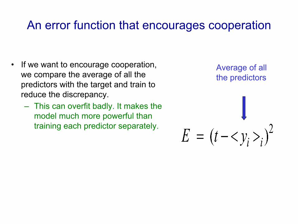
• If we want to encourage cooperation, we compare the average of all the predictors with the target and train to reduce the discrepancy.– This can overfit badly. It makes the

model much more powerful than training each predictor separately.

Average of all the predictors

An error function that encourages specialization

• If we want to encourage specialization we compare each predictor separately with the target.

• We also use a “manager” to determine the probability of picking each expert.– Most experts end up ignoring most

targets

probability of the manager picking expert i for this case

The mixture of experts architecture (almost)

A simple cost function :

Expert 1 Expert 2 Expert 3

input

Softmax gating network

There is a better cost function based on a mixture model.

The derivatives of the simple cost function

• If we differentiate w.r.t. the outputs of the experts we get a signal for training each expert.

• If we differentiate w.r.t. the outputs of the gating network we get a signal for training the gating net.– We want to raise p for all

experts that give less than the average squared error of all the experts (weighted by p)

A better cost function for mixtures of experts(Jacobs, Jordan, Nowlan & Hinton, 1991)

• Think of each expert as making a prediction that is a Gaussian distribution around its output (with variance 1).

• Think of the manager as deciding on a scale for each of these Gaussians. The scale is called a “mixing proportion”. e.g {0.4 0.6}

• Maximize the log probability of the target value under this mixture of Gaussians model i.e. the sum of the two scaled Gaussians.

t target value

y2y1

The probability of the target under a mixture of Gaussians

prob. of target value on case c given the mixture.

mixing proportion assigned to expert i for case c by the gating network

output of expert i

normalization term for a Gaussian with

The idea of full Bayesian learning

Full Bayesian Learning• Instead of trying to find the best single setting of the parameters (as

in Maximum Likelihood or MAP) compute the full posterior distribution over all possible parameter settings.– This is extremely computationally intensive for all but the

simplest models (its feasible for a biased coin).• To make predictions, let each different setting of the parameters

make its own prediction and then combine all these predictions by weighting each of them by the posterior probability of that setting of the parameters.– This is also very computationally intensive.

• The full Bayesian approach allows us to use complicated models even when we do not have much data.

Overfitting: A frequentist illusion?

• If you do not have much data, you should use a simple model, because a complex one will overfit. – This is true. – But only if you assume that

fitting a model means choosing a single best setting of the parameters.

• If you use the full posterior distribution over parameter settings, overfitting disappears.– When there is very little

data, you get very vague predictions because many different parameters settings have significant posterior probability.

A classic example of overfitting

• Which model do you believe?– The complicated model fits the

data better.– But it is not economical and it

makes silly predictions.• But what if we start with a reasonable

prior over all fifth-order polynomials and use the full posterior distribution.– Now we get vague and sensible

predictions. • There is no reason why the amount of

data should influence our prior beliefs about the complexity of the model.

Approximating full Bayesian learning in a neural net

• If the neural net only has a few parameters we could put a grid over the parameter space and evaluate p( W | D ) at each grid-point.– This is expensive, but it does not involve any gradient descent

and there are no local optimum issues.• After evaluating each grid point we use all of them to make

predictions on test data– This is also expensive, but it works much better than ML learning

when the posterior is vague or multimodal (this happens when data is scarce).

An example of full Bayesian learning

• Allow each of the 6 weights or biases to have the 9 possible values -2, -1.5, -1, -0.5, 0 ,0.5, 1, 1.5, 2

– There are grid-points in parameter space • For each grid-point compute the probability of the

observed outputs of all the training cases. • Multiply the prior for each grid-point by the

likelihood term and renormalize to get the posterior probability for each grid-point.

• Make predictions by using the posterior probabilities to average the predictions made by the different grid-points.

bias

bias

A neural net with 2 inputs, 1 output and 6 parameters

Making full Bayesian learning practical

What can we do if there are too many parameters for a grid?

• The number of grid points is exponential in the number of parameters.– So we cannot deal with more than a few parameters using a grid.

• If there is enough data to make most parameter vectors very unlikely, only a tiny fraction of the grid points make a significant contribution to the predictions.– Maybe we can just evaluate this tiny fraction

• Idea: It might be good enough to just sample weight vectors according to their posterior probabilities.

Sample weight vectors with this probability

Sampling weight vectors

• In standard backpropagation we keep moving the weights in the direction that decreases the cost.– i.e. the direction that

increases the log likelihood plus the log prior, summed over all training cases.

– Eventually, the weights settle into a local minimum or get stuck on a plateau or just move so slowly that we run out of patience.

weight space

One method for sampling weight vectors

• Suppose we add some Gaussian noise to the weight vector after each update.– So the weight vector never

settles down.– It keeps wandering around,

but it tends to prefer low cost regions of the weight space.

– Can we say anything about how often it will visit each possible setting of the weights?

weight space

Save the weights after every 10,000 steps.

The wonderful property of Markov Chain Monte Carlo

• Amazing fact: If we use just the right amount of noise, and if we let the weight vector wander around for long enough before we take a sample, we will get an unbiased sample from the true posterior over weight vectors.– This is called a “Markov Chain

Monte Carlo” method.– MCMC makes it feasible to use

full Bayesian learning with thousands of parameters.

• There are related MCMC methods that are more complicated but more efficient:– We don’t need to let the

weights wander around for so long before we get samples from the posterior.

Full Bayesian learning with mini-batches

• If we compute the gradient of the cost function on a random mini-batch we will get an unbiased estimate with sampling noise.– Maybe we can use the

sampling noise to provide the noise that an MCMC method needs!

• Ahn, Korattikara &Welling (ICML 2012) showed how to do this fairly efficiently.– So full Bayesian learning is

now possible with lots of parameters.

Dropout: an efficient way to combine neural

nets

Two ways to average models

• MIXTURE: We can combine models by averaging their output probabilities:

• PRODUCT: We can combine models by taking the geometric means of their output probabilities:

Model A: .3 .2 .5

Model B: .1 .8 .1

Combined .2 .5 .3

Model A: .3 .2 .5

Model B: .1 .8 .1

Combined .03 .16 .05 /sum

Dropout: An efficient way to average many large neural nets (http://arxiv.org/abs/1207.0580)

• Consider a neural net with one hidden layer.

• Each time we present a training example, we randomly omit each hidden unit with probability 0.5.

• So we are randomly sampling from 2^H different architectures.– All architectures share weights.

Dropout as a form of model averaging

• We sample from 2^H models. So only a few of the models ever get trained, and they only get one training example.– This is as extreme as bagging can get.

• The sharing of the weights means that every model is very strongly regularized.– It’s a much better regularizer than L2 or L1 penalties that pull the

weights towards zero.

But what do we do at test time?

• We could sample many different architectures and take the geometric mean of their output distributions.

• It better to use all of the hidden units, but to halve their outgoing weights.– This exactly computes the geometric mean of the predictions of

all 2^H models.

What if we have more hidden layers?

• Use dropout of 0.5 in every layer.• At test time, use the “mean net” that has all the outgoing weights

halved.– This is not exactly the same as averaging all the separate

dropped out models, but it’s a pretty good approximation, and its fast.

• Alternatively, run the stochastic model several times on the same input. – This gives us an idea of the uncertainty in the answer.

What about the input layer?

• It helps to use dropout there too, but with a higher probability of keeping an input unit.– This trick is already used by the “denoising autoencoders”

developed by Pascal Vincent, Hugo Larochelle and Yoshua Bengio.

How well does dropout work?

• The record breaking object recognition net developed by Alex Krizhevsky (see lecture 5) uses dropout and it helps a lot.

• If your deep neural net is significantly overfitting, dropout will usually reduce the number of errors by a lot.– Any net that uses “early stopping” can do better by using dropout

(at the cost of taking quite a lot longer to train). • If your deep neural net is not overfitting you should be using a bigger

one!

Another way to think about dropout

• If a hidden unit knows which other hidden units are present, it can co-adapt to them on the training data. – But complex co-adaptations

are likely to go wrong on new test data.

– Big, complex conspiracies are not robust.

• If a hidden unit has to work well with combinatorially many sets of co-workers, it is more likely to do something that is individually useful.– But it will also tend to do

something that is marginally useful given what its co-workers achieve.